LOW-LYING EXCITED ENERGY STATES AND STRUCTURE OF DEFORMED NUCLEI

NOORA BINTI ROSLI

DISSERTATION SUBMITTED IN FULFILMENT OF THE REQUIREMENT FOR THE DEGREE OF

MASTER OF SCIENCE

FACULTY OF SCIENCE UNIVERSITY OF MALAYA

KUALA LUMPUR

2013

iii

ABSTRACT

Low-lying excited states and structure of even-even, deformed, rare earth

Sm,, 156154152 and Dy,,,,, 166164162160158156

nuclei are studied. A phenomenological model

is used to understand the properties of deformed nuclei. The experimental data are

analyzed by theoretical analysis within this model. Major steps in the derivation

of cranking model are briefly presented. Harris parameterization for the energy

and angular momentum are formulated and analyzed. The inertial parameters for

the even-even deformed nuclei are defined using the Harris parameterization. The

angular frequency of rotation is derived from the cubic equation of angular

momentum. The values of angular frequency )(Irotω and rotational energy

)(IErot are calculated for the Sm,, 156154152 and Dy,,,,, 166164162160158156 nuclei at low

spin h10≤I . The energy spectra of positive-parity states which are in good

agreement with the experimental data are presented. Few new states that are not

available in the experimental data are predicted. At higher total angular

momentum, deviation from the adiabatic theory is shown by the increment of

energy difference between theoretical and experimental values. It is found that the

non-adiabaticity of rotational energy bands occurred at high spin due to the

Coriolis effect. The parameters fitted to the model are calculated. The complete

low energy structures of Sm,, 156154152 and Dy,,,,, 166164162160158156 isotopes are

calculated by taking into account the Coriolis mixing between states. The effect of

+= νπ 1K bands on low-lying )0( 1

+=πK ground states, 1β −= + )0( 2πK , 2β

iv

−= + )0( 3πK , and γ −= + )2( πK bands is studied. Larger values of Coriolis

interaction matrix elements, ',)(

KKxj and the closeness between band head

energies, Kω induce strong states mixing.

v

ABSTRAK

Keadaan teruja paras rendah dan struktur bahagian nukleus tercangga genap-

genap nadir bumi Sm,, 156154152 dan Dy,,,,, 166164162160158156 dikaji. Model

fenomenologi digunakan untuk memahami sifat nukleus tercangga. Data

eksperimen dianalisis secara teori dalam model ini. Langkah-langkah utama

dalam penerbitan model “cranking” dibentangkan secara ringkas. Parameterisasi

Harris untuk tenaga dan momentum sudut dirumuskan dan dianalisis. Parameter

inersia untuk nukleus tercangga genap-genap ditakrifkan dengan menggunakan

parameterisasi Harris. Frekuensi sudut putaran diterbitkan daripada persamaan

kuasa tiga momentum sudut. Nilai-nilai frekuensi sudut )(Irotω dan tenaga

putaran )(IErot dikira untuk nukleus Sm,, 156154152 dan Dy,,,,, 166164162160158156 pada spin

rendah h10≤I . Spektrum tenaga keadaan berpariti positif yang bersetuju dengan

baik dengan data eksperimen dibentangkan. Beberapa keadaan baru yang tidak

terdapat di dalam data eksperimen diramalkan. Pada jumlah momentum sudut

yang lebih tinggi, sisihan daripada teori adiabatik ditunjukkan oleh peningkatan

beza tenaga antara nilai teori dan eksperimen. Ketidak-adiabatikan jalur tenaga

putaran di dapati berlaku pada spin tinggi kerana kesan Coriolis. Parameter yang

disesuaikan dalam model tersebut dikira. Struktur tenaga rendah isotop

Sm,, 156154152 dan Dy,,,,, 166164162160158156 yang lengkap dikira dengan mengambil kira

campuran Coriolis antara keadaan-keadaan. Kesan jalur += νπ 1K ke atas jalur-

jalur keadaan dasar )0( 1+=πK ,

dan 1β )0( 2

+=πK , 2β )0( 3+=πK , γ )2( +=πK

vi

dikaji. Nilai elemen matriks saling tindakan Coriolis ( ) ',KKxj yang besar dan

kedekatan di antara tenaga kepala jalur Kω mengaruhkan campuran keadaan yang

kuat.

vii

ACKNOWLEDGEMENTS

I praise and thank God for His grace in giving me strength to complete this

project. And for the successful completion of my Master of Science project, I

would like to express my sincere appreciations to many people for the motivation

and support I have received.

In the first place, I would like to address my acknowledgements to my first

supervisor, Assoc. Prof. Dr. Hasan Abu Kassim for his various suggestions and

criticism throughout all stages of the research project. I am deeply thankful to my

co-supervisor Dr. Abdurahim A. Okhunov for his valuable advice and guidance

throughout the research project. He was never reluctant to assist despite his

workload.

I am much indebted to Azni Abdul Aziz, Nor Sofiah Ahmad and the Theoretical

Physics Research Group who have contributed, maybe unintentionally, to

technically help and continuously guide in each step of my project. I would like to

express my sincere gratitude to all my friends, who prevented frustration from

creeping in.

To my grandparents, my father, my mother, my family and my dearest, this

achievement is my gift to you. It was great to know that you have been around

when I needed you. You have believed in me and have given me a grasp of my

viii

own self-worth. My love to all of you that keeps me going. It derives my strength

and inspiration. I love you all!

Last but not least, I would also like to thank University of Malaya for providing

scholarship throughout my MSc. research project.

ix

TABLE OF CONTENTS

ORIGINAL LITERARY WORK DECLARATION ii

ABSTRACT iii

ABSTRAK v

ACKNOWLEDGEMENTS vii

TABLE OF CONTENTS ix

LIST OF FIGURES xi

LIST OF TABLES xiv

1 INTRODUCTION

1.1 Rare-Earth Elements : Samarium-62 and Dysprosium-66 1

1.2 Even-even Nuclei 4

1.3 Collective Characteristic of Deformed Nuclei 5

1.4 Objectives 7

1.5 Organization of Thesis 8

2 NUCLEAR MODELS

2.1 The Liquid Drop Model: Semi-Empirical Mass Formula 10

2.2 Spherical Shell Model 16

2.3 Nuclear Collective Model 20

2.3.1 Vibration 22

2.3.2 Deformation 24

2.3.3 Axially Symmetric Ellipsoid Shape 28

x

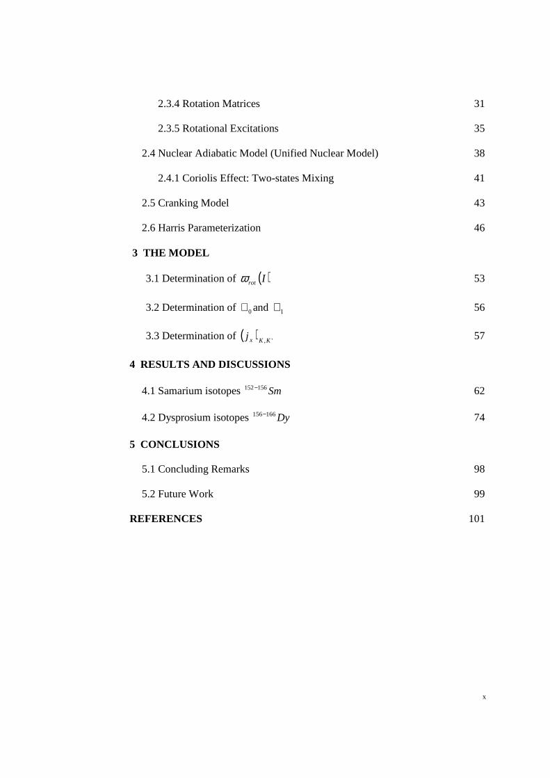
2.3.4 Rotation Matrices 31

2.3.5 Rotational Excitations 35

2.4 Nuclear Adiabatic Model (Unified Nuclear Model) 38

2.4.1 Coriolis Effect: Two-states Mixing 41

2.5 Cranking Model 43

2.6 Harris Parameterization 46

3 THE MODEL

3.1 Determination of ( )Irotω 53

3.2 Determination of 0ℑ and 1ℑ 56

3.3 Determination of ( ) ',KKxj 57

4 RESULTS AND DISCUSSIONS

4.1 Samarium isotopes Sm156152− 62

4.2 Dysprosium isotopes Dy166156− 74

5 CONCLUSIONS

5.1 Concluding Remarks 98

5.2 Future Work 99

REFERENCES 101

xi

LIST OF FIGURES

1.1 Samarium-62 2

1.2 Dysprosium-66. 3

1.3 Energies of lowest 2+ states in even-even nuclei. The lines connect

sequences of isotopes. 4

1.4 Reduced Transition Probabilities B(E2) for lowest 2⁺ states of even-even

nuclei. 5

1.5 Energy ratio ++ 24/ EE for excitation of lowest 2+ and 4+ states in even-even

nuclei. The lines connect sequences of isotopes . 6

1.6 Work structure in the research. 8

2.1 Binding energy per nucleon along the stability line. 12

2.2 The contributions of various terms in the semiempirical mass formula to the

binding energy per nucleon. 13

2.3 The plot of N versus Z for all stable nuclei. 14

2.4 Deviation of the experimental values of the binding energy per nucleon from

the semi-empirical values. The solid curve represents the semi-empirical

binding energy formula, Equation 2.3 and the open circles are the

experimental data. 15

2.5 The Wood-Saxon potential. 19

2.6 The coupling between the spin angular momentum and orbital angular

momentum. 20

2.7 The magic number configuration reproduced by spin-orbit interaction. 21

xii

2.8 A vibrating nucleus with spherical equilibrium shape. 23

2.9 Modes of nuclear vibration. 24

2.10 Nuclear shapes in the principal axes system as a function ofγ for fixed

β . 26

2.11 Nuclear shapes in relation with eccentricity, 2β . 27

2.12 Nuclear shapes in relation with electric quadrupole moment, Q . 27

2.13 Coupling scheme for particle in slowly rotating spheroidal nucleus in 2-D

coordinate system. 29

2.14 The rotational angular momentum is not along the symmetry axis and

the intrinsic angular momentum is assumed to be zero, for simplicity. 30

2.15 Rotation of the coordinate axes from ,(x ,y )z to )',','( zyx by Euler

angles ),,( γβα in three steps. 32

2.16 Relationship between the total angular momentum, Ir

, the intrinsic angular

momentum, Jr

, the rotational angular momentum, Rr

and the component

of Ir

along the laboratory-fixed z axis, M and the symmetry axis in the

body-fixed frame, K . 33

2.17 Rotational band built upon the ground state of a deformed, even-even

nucleus in the rigid rotor approximation. 36

2.18 Energy ratio in the ground band state in the even-even nuclei in the

152 < A< 186. Data were taken from (Firestone et al. 1996). 38

2.19 Two-level mixing. 42

2.20 Moments of inertia in rare earth nuclei. 46

xiii

4.1 The linear dependencies of )(IJ eff on )(2 Ieffω . 62

4.2 The linear dependencies of )(IJ eff on )(2 Ieffω . 63

4.3 The linear dependencies of )(IJ eff on )(2 Ieffω . 64

4.4 Energy spectrum of positive-parity states of Sm152isotope. 70

4.5 Energy spectrum of positive-parity states of Sm154isotope. 71

4.6 Energy spectrum of positive-parity states of Sm156isotope. 72

4.7 The linear dependencies of )(IJ eff on )(2 Ieffω . 74

4.8 The linear dependencies of )(IJ eff on )(2 Ieffω . 75

4.9 The linear dependencies of )(IJ eff on )(2 Ieffω . 76

4.10 The linear dependencies of )(IJ eff on )(2 Ieffω . 77

4.11 The linear dependencies of )(IJ eff on )(2 Ieffω . 78

4.12 The linear dependencies of )(IJ eff on )(2 Ieffω . 79

4.13 Energy spectrum of positive-parity states of Dy156 isotope. 90

4.14 Energy spectrum of positive-parity states of Dy158 isotope. 91

4.15 Energy spectrum of positive-parity states of Dy160 isotope. 92

4.16 Energy spectrum of positive-parity states of Dy162 isotope. 93

4.17 Energy spectrum of positive-parity states of Dy164 isotope. 94

4.18 Energy spectrum of positive-parity states of Dy166 isotope. 95

xiv

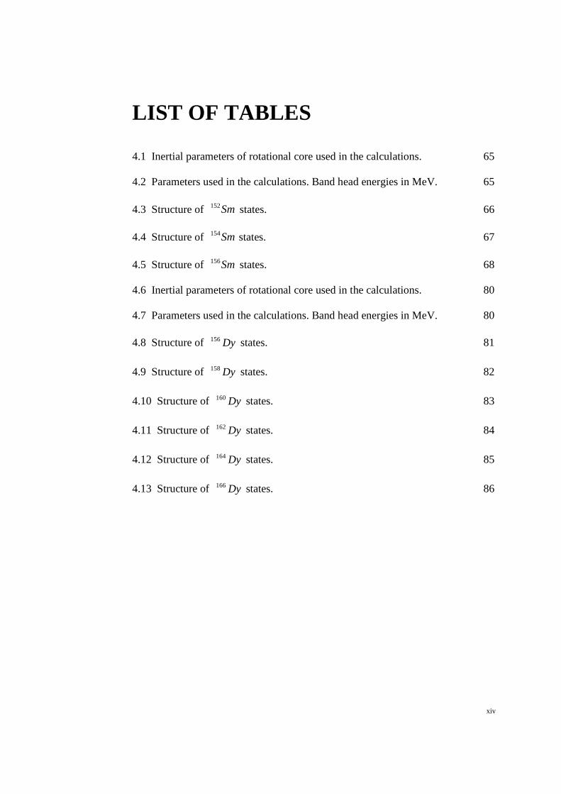
LIST OF TABLES

4.1 Inertial parameters of rotational core used in the calculations. 65

4.2 Parameters used in the calculations. Band head energies in MeV. 65

4.3 Structure of Sm152 states. 66

4.4 Structure of Sm154 states. 67

4.5 Structure of Sm156 states. 68

4.6 Inertial parameters of rotational core used in the calculations. 80

4.7 Parameters used in the calculations. Band head energies in MeV. 80

4.8 Structure of Dy156 states. 81

4.9 Structure of Dy158 states. 82

4.10 Structure of Dy160 states. 83

4.11 Structure of Dy162 states. 84

4.12 Structure of Dy164 states. 85

4.13 Structure of Dy166 states. 86

1

CHAPTER 1

INTRODUCTION

1.1 Rare-Earth Elements: Samarium and Dysprosium

Separated from the main body of the periodic table, one can see two rows of

elements below the main body chart. These elements which include the

lanthanides and actinides are called rare earth elements in the mass region of

190150 << A . There are few opinions of the “rare” term. Some sources state

that these elements are rare due to their scarcity [1-2]. The rare earth elements

are typically dispersed and very difficult to find in concentrated form. The

rarest rare earth metals are more abundant than gold, silver and lead. It took

long and tedious processes to purify the metals from their oxides. But, the ion-

exchange and solvent extraction processes used today which are low in cost

can produce purer metals in short time [3-4].

There are common properties that can be applied on all of the rare earth

elements. They appear as silvery-white or gray metals that have high luster. In

air, these elements are very easy to oxide. The metals are very good electric

conductors and have magnetic properties due to magnetic moment. Because of

these common properties, it is very difficult to distinguish these elements from

one another. Furthermore, they occur together in minerals naturally, e.g. in

monazite sand. The elements themselves are not radioactive, but they are

found in ore containing thorium and uranium.

Rare earth metals are vital to high-tech manufacturing. These metals are used

in most electronic devices. Powerfulness and efficiency plus less in weight and

2

ability to pack energy in smaller space are the reasons why most electronic

devices become smaller [2, 5].

Samarium and Dysprosium are categorized as lanthanides. They are quite well

studied experimentally and theoretically [6-32]. Samarium is a fairly hard,

pale silvery white metal as shown in Figure 1.1. Samarium has 30 known

isotopes and the stable isotopes include Sm144 , Sm150 , Sm152 and Sm154 . The

element Sm152 is the most abundant isotope with %.7526 natural abundance.

The element Sm148 is extremely long-lived radioisotopes with half-life of

15107× yr. The naturally occurring element Sm146 is also fairly long-lived

radioisotopes with half-life of 810031 ×. yr. The long lived isotopes, Sm146

and Sm148 are primarily decayed by alpha decay to isotopes of neodymium.

Figure 1.1 Samarium [33].

Samarium can ignite in dry air if heated above o150C and form oxide coating

if not stored in inert gas. Main application of the samarium is in samarium-

3

cobalt alloy magnets in electronic devices due to its high resistance to

demagnetization and its ability to operate at high temperature up to o700 C.

The long-lived radioisotopes of samarium are used in samarium-neodymium

dating for determining the age relationships of rocks and meteorites [34-35].

Figure 1.2 Dysprosium [33].

Dysprosium is a soft and silvery-white rare earth metal as pictured in Figure

1.2. The stable isotopes of Dysprosium elements include Dy156 , Dy158 , Dy160 ,

Dy162 and Dy164 . The most abundant isotope is Dy164 at %.1828 . This metal

reacts with cold water and dissolves in both dilute and concentrated acids.

Dysprosium is an excellent neutron absorber that it is used in dysprosium-

oxide-nickel cement in control rods in nuclear reactors. In addition,

Dysprosium is used in data storage applications such as compact discs and

hard discs [36].

4

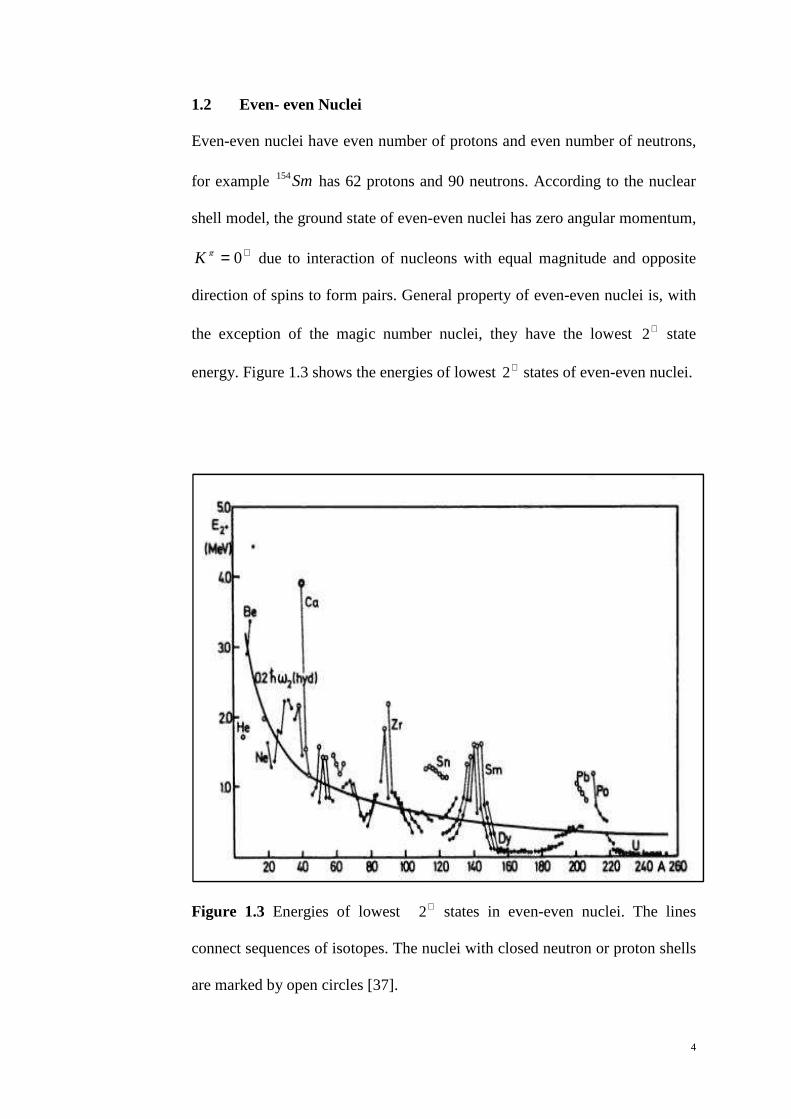
1.2 Even- even Nuclei

Even-even nuclei have even number of protons and even number of neutrons,

for example Sm154 has 62 protons and 90 neutrons. According to the nuclear

shell model, the ground state of even-even nuclei has zero angular momentum,

+= 0πK due to interaction of nucleons with equal magnitude and opposite

direction of spins to form pairs. General property of even-even nuclei is, with

the exception of the magic number nuclei, they have the lowest +2 state

energy. Figure 1.3 shows the energies of lowest +2 states of even-even nuclei.

Figure 1.3 Energies of lowest +2 states in even-even nuclei. The lines

connect sequences of isotopes. The nuclei with closed neutron or proton shells

are marked by open circles [37].

5

1.3 Collective Characteristic of Deformed nuclei

The isotopes Sm,, 156154152 and Dy,,,,, 166164162160158156

are classified as deformed

nuclei. The valence nucleons of these deformed nuclei achieve low energy

state for stability. Rotational and vibrational energy levels exist in these nuclei

as they have nonspherically symmetric potential that is sensitive to collective

motions. The collective characteristic of even-even deformed nuclei can be

indicated by larger value of reduced transition probabilities, );E(B ++ → 202

and constant value of energy ratio for the excitation of lowest +4 and +2

states, 33324

.E/E =++ . Rotation of a deformed charged object will emit

electric quadrupole 2E radiation. The value 33324

.E/E =++ is equal to that

of the pure rigid rotator value. Figures 1.4 and 1.5 show the remarkable

Figure 1.4 Reduced Transition Probabilities B(E2) for lowest +2 states of

even-even nuclei [38].

6

Figure 1.5 Energy ratio ++ 24E/E for excitation of lowest +2 and +4 states in

even-even nuclei. The lines connect sequences of isotopes [39].

behavior of nuclei in the rare earth mass regions which is consistent with the

behavior of nuclei possessing large deformations.

Bohr and Mottelson suggested a theoretical direction to describe the deformed

nuclei [40-41]. Nuclear behavior is predicted by angular frequency, moment of

inertia and angular momentum induced by rotation.

For small values of angular momentum I , the rotational energy is expanded as

a function of )I(I 1+ :

( )( ) ...)I(CI)I(BI)I(AIIIErot ++++++=+ 3322 1111

7

But, this law of )I(I~Erot 1+ is invalidate at high values of I . Prior to this

weakness, more advance knowledge is explored to improve the understanding

and explanation of nuclear behavior.

Nuclei as we know, made up of two different types of nucleons, i.e. protons

and neutrons. These nucleons, as described by two-rotor model have dipole

vibrational modes in which they oscillate around common axis in opposite

phases. The oscillations generate isovector magnetic dipole resonance. The

low-lying, collectively magnetic dipole excitations in deformed nuclei were

discovered in the last decade [42]. Since then, interest to study the properties

of the deformed nuclei has increased especially in the last few years [43-50]. It

is evidently to state that the low-lying +1 states spread around the excitation

energy of 3 MeV in energy spectrum [51].

Taking into account the Coriolis mixing of the isovector collective M1 states

with low-lying states will lead for the non-adiabaticity of electromagnetic

properties to occur [52-54].

1.4 Objectives

This study has two objectives:

1. To predict the energy spectra and study the low-lying excited

energy states of Sm,, 156154152 and Dy,,,,, 166164162160158156 isotopes.

2. To analyze the wave function structure of nuclear band states of

Sm,, 156154152 and Dy,,,,, 166164162160158156 isotopes.

8

The basic states of the Hamiltonian include ( )+= 10πK ground state band,

( )−= +21 0πKβ , ( )−= +

32 0πKβ , ( )−= +2πKγ vibrational bands and

+= ν

πK 1 collective states (ν is the number of +1 collective states).

1.5 Organization of Thesis

This thesis contains five chapters. The following chapter presents the overall

theoretical and literature review done throughout the research. The description

of nuclear models, the concepts of deformed nuclei, and the derivation of

Harris parameterization from the cranking model are covered in Chapter 2.

The calculation and methodology of this study are demonstrated in Chapter 3.

The structural work involving the analytical part is outlined with a flowchart

presented in Figure 1.6.

Figure 1.6 Work structure in the research.

9

Chapter 4 presents the results of the research. The results obtained for the

determinations of inertial parameters, headband energies and the matrix

elements of Coriolis mixing for Sm,, 156154152 and Dy,,,,, 166164162160158156 nuclei

are presented in this chapter. The calculated values of the energy of low-

lying excited states and the wave function structures of the nuclei are also

included in this chapter. The explanations regarding the results obtained

are discussed.

The final chapter summarizes the overall work done and concludes the

study of low-energy structure in Sm,, 156154152 and Dy,,,,, 166164162160158156 nuclei.

On-going and future works that may be explored are also included at the

end of this chapter.

10

CHAPTER 2

NUCLEAR MODELS

The main problem of nuclear physics is to understand and explain the complex

interaction in a nucleus. By 1934, scientists had found that the nucleus consists

of protons and neutrons, but they did not have so much idea what is the

general shape of nucleus and how these particles arrange themselves.

The nucleons inside an atomic nucleus are categorized as many-particle

system that held by their mutual interaction via electromagnetic and strong

forces. We are dealing with many-body problem of great complexity. Nuclear

model is a simple way to look into a nucleus to give a wide range of its

properties possible. A model is successful if it has the ability to predict

measured nuclear properties that can be verified experimentally in the

laboratory. The results predicted by the model must also be in good agreement

with previous results. This chapter presents the chronology of nuclear model

development relevant to this research.

2.1 The Liquid Drop Model: Semi-Empirical Mass Formula

A nucleus is not a simple collection of nucleons. In a reaction between A and

b , there is an intermediate step C that delays the emission of particles X and

y .

yXCbA * +→→+

A Danish physicist, Niels Bohr proposed in the intermediate step, the energy is

distributed among all nucleons and ends up on the emitted particles [55]. In

11

this model, the nucleons interacting via internal strong forces with their

nearest neighbors in short range and results in the constantly oscillating and

changing shape of the nucleus. In this respect, the nucleus is incompressible

and not rigid as water droplet. As a consequence, the liquid drop model was

suggested as early collective model in which the individual quantum

properties of nucleons are completely ignored.

If two neighboring nucleons interact with each other, the total mass of the

system is less than the sum of all the mass of individual nucleons. The mass

defect is the difference in mass of the nucleus and its constituent nucleons; Z

protons and N neutrons. The mass defect is defined by:

( ) ( )N,ZMNMZM np −+=∆ (2.1)

where pM and nM are the mass of the proton and neutron respectively. The

stronger the interaction, the more the mass decreases.

To see how strong the nucleons are bound together, the mass defect is

converted to the mass-energy equivalence which is the nuclear binding energy.

The nuclear binding energy is given by:

( ) ( ) ( )[ ] 2cN,ZMNMZMN,ZB NP −+= . (2.2)

The experimental nuclear binding energies of a wide range of nuclides are

plotted in Figure 2.1. Binding energies per nucleon increase sharply as A

reaches the peak of ~ 8 MeV/nucleon at iron (Fe) and then decreasing slowly

12

for the more massive nuclei. Above this value, the average binding energy per

nucleon, A/B is relatively constant indicating that the nuclear density is

almost constant and the nuclear force exhibits saturation properties.

Figure 2.1 Binding energy per nucleon along the stability line [56].

On the basis of the liquid drop model, a systematic study leads to the

completion of nuclear binding energy formula with few terms that shows the

collective and the individual nucleons features of nuclei. Figure 2.2 shows the

contribution of the correction terms in the semi-empirical formula:

( ) ( ) ( )δ

A

ZAaAZZaAaAaA,ZB symcsv +−−−−−=

− 2

3

1

3

2 21 . (2.3)

13

The Aav term is proportional to the nuclear volume and represents the

volume energy for the case of constant saturated binding energy per nucleon at

8 MeV. The 3

2

Aas term corrects the binding energy formula due to the surface

Figure 2.2 The contributions of various terms in the semiempirical mass

formula to the binding energy per nucleon [57].

effect. The nucleons at the surface layer do not contribute to the binding

energy as much as those in the central region. As in the raindrop, the force in

the central core is saturated but drops to zero at the surface [58]. For lighter

nuclei, the binding energy per nucleon is smaller because of larger surface-to-

volume ratio.

The ( ) 3

1

1−

− AZZac term is due to Coulomb repulsion between the Z protons in

the nucleus. This Coulomb energy has destabilizing effect that reduces the

binding strength. This term is very important for heavy nuclei because

14

additional neutrons are required for nuclear stability. The A

)ZA(asym

22− term

is called symmetry energy. Unlike the Coulomb energy term, this term is

important for light nuclei, for which 2/ANZ == is strictly observed as

presented in Figure 2.3.

Figure 2.3 The plot of N versus Z for all stable nuclei [59].

The last term is called the pairing energy. This is due to nucleons tendency to

form pairs with zero spin. When the value of both numbers of neutron and

proton are odd, the odd proton is converted into a neutron (or vice versa), so

that it gains binding energy to form a pair with its formerly odd partner. The

pairing energy term of odd number of neutron and proton is subtracted from

15

the binding energy formula as opposed to that of the nuclei with even number

of neutron and proton, which have greater stability. For nuclei with odd

nucleon number, this term is taken as zero because such nuclei can be

described without the last term.

The parameters va , sa , ca and syma are adjusted to give the best agreement

with the experimental curve. By using this expression for B , the semi-

empirical mass formula is formulated which is regarded as a first attempt to

apply nuclear models. Since nucleons are bound, the binding energy must be

subtracted from the total mass:

. ( ) ( ) 2c/N,ZBNMZMA,ZM NP −+= . (2.4)

Figure 2.4 Deviation of the experimental values of the binding energy per

nucleon from the semi-empirical values. The solid curve represents the semi-

empirical binding energy formula, Equation (2.3) and the open circles are the

experimental data [37].

16

However, it is proven in Figure 2.4 that the experimental values deviate from

that of semi-empirical formula with large nuclear binding energy at certain

number of neutrons and protons. These numbers are called the magic numbers

of nuclei.

2.2 Spherical Shell Model

Nuclear shell model is obtained by analogous comparison with atomic shell

model. The shell model accounts for many features of energy levels. In the

atomic shell model, the shells are filled with electrons in increasing order of

energy. Finally, the inert core of filled shells and valence electrons are

obtained. The atomic properties are then determined by the valence electrons.

This concept is applied on the nucleons in the nucleus. Some measured

nuclear properties are remarkably in agreement with the prediction of the

model.

The motion of each nucleon is governed by the average attractive force of all

other nucleons. The resulting orbits of moving nucleons form shells. By Pauli

Exclusion Principle, each nucleon is assigned a unique set of quantum

numbers to describe its motion. The nucleons fill the lowest-energy shells as

permitted by this principle. If the shells are fully filled, a nucleus would show

unusual stability. Magic number represents shell closure occurs at proton and

neutron numbers of 2, 8, 20, 28, 50, 82 and 126. These filled shells have total

angular momentum += 0πJ . The next added nucleon, the valence nucleon

determines the πJ of the new ground state. Thus, the shell model describes the

energy required to excite nucleons and how the quantum numbers change.

17

However, there are some differences between the atom and nucleus. The well-

known properties of atoms are the electrons move independently in an average

atomic potential. Unlike the electrons, nucleons move in an average potential

generated by other nucleons. Regarding large diameter of the nucleons relative

to the nucleus itself, how can the nucleons move in well defined orbits without

any collisions? The mean free path of a nucleon is very short compared to the

length of its orbit. This objection can be encountered by the explanation of the

Pauli Exclusion Principle and how the shells are filled. The collisions involve

the energy transfer of nucleons to one another. Nucleon that gains energy must

excite to the nearby levels but the filled shells cannot accept additional

nucleons. To move up to the valence band, more energy is required than the

transferred energy during collisions. Therefore, the collisions cannot occur,

and the nucleons orbit as if they were transparent to one another.

In developing the shell model, the ordering and energy of the nuclear states

can be calculated by solving the three-dimensional Schrodinger equation:

( ) ( )rψE)r(ψrVm

vrh =

+− ∆

2

2

. (2.5)

Assuming a nucleon moves in a spherical potential with spherical coordinates

,r( ,θ )ϕ using the relations

22

2

2

2 12

h

r

r

l

rrr−

∂∂+

∂∂=∆ (2.6)

and ,(θlr

)ϕ is the angular momentum operator such that

22

2

22

sin

1sin

sin

1h

r

∂∂+

∂∂

∂∂−=

ϕθθθ

θθl . (2.7)

By applying variables separation method, a wave function having radial and

angular parts is obtained. The number of radial nodes n is the principle

18

quantum number. The angular part is spherical harmonic ( )φ,θY ml

with

quantum numbers l and m corresponding to the angular momentum of the state

and the projection of the angular momentum onto an axis. Solutions obtained

are similar to the 3-dimensional harmonic oscillator.

Another more realistic potential to describe the forces applied on each nucleon

is Wood-Saxon potential:

( ) ( )[ ]a/Rrexp

VrV

−+−=

10 (2.8)

where potential well depth, 500 ≈V MeV, nuclear radius, 3121 /A.R −= fm,

and a representing the surface thickness of the nucleus, 50 .a = fm.

The Wood-Saxon potential illustrated in Figure 2.5 is based on the assumption

that each nucleon moves in an average interaction with all other nucleons. The

force is attractive at increasing distance. When Rr ≈ within a , the force

towards the center is large. If aRr >>− , which means ∞→r , the force

rapidly approaching zero indicating the nature of short-distance of strong

force.

However, if all the nucleons filled the particular states according to Pauli

Exclusion Principle, the counted nucleons only agreed for the first three magic

numbers. The prediction fails to fit the experimental observation. In 1949,

Mayer and Jensen pointed out independently that the average potential felt by

individual nucleons must include the spin-orbit term, slv

v

• [60].

19

Figure 2.5 The Wood-Saxon potential [61].

The applicable potential is:

( ) ( ) slalβrωmrUv

v

•++−= 22

2

1 . (2.9)

The first term is the harmonic oscillator potential. The correct sequence of

“magic numbers” is not reproduced by this potential. Only the first three

magic number, 2, 8, and 20 emerging from this scheme. The individual

nucleon not only interacts with all other nucleons, but also with itself. A

nucleon is orbiting and also rotating. In Figure 2.6, we see that the spin

angular momentum parallel to the orbital angular momentum is favored. Each

nucleon orbit is split into two components, labeled by the total spin sljv

vv

+= .

All jv

for all nucleons will give the resultant angular momentum ( jj −

coupling). However, this nuclear spin-orbit coupling is different from the one

exists in atoms where total orbital angular momentum of all electrons, Lr

,

combine with total of all spins Sr

to form Jr

.

20

Figure 2.6 The coupling between the spin angular momentum and orbital

angular momentum [62].

The introduction of the spin-orbit interaction is able to explain the

experimental shell closure at 2, 8, 28, 50, 82, and 126 as pictured in Figure

2.7.

2.3 Nuclear Collective Model

For closed-shells configuration, the nucleus tends to be spherical. The addition

of one or more nucleons produces small deformation. The nuclear shell model

can explain this situation successfully. However, for the nuclei in the region

21

(rare-earths and actinides), the departing from the spherical shape cannot be

ignored.

Figure 2.7 The magic number configuration reproduced by spin-orbit

interaction [60].

The collective model proposed by Bohr and Mottelson [40], is inspired by the

liquid drop model and the Rainwater proposal [63] about the intrinsically

deformation of most nuclei away from closed shells with prolate quadrupole

shape. The whole nucleus is deformed by single-particle motions and the

observed electric quadrupole moment, Q is because of collective orbital

distortions.

22

Analogous to liquid-drop idea, a nucleus consists of filled-shells as inner core

and the outer valence nucleons as the surface of the liquid drop. In addition to

the motion of individual nucleons, all the nucleons in the nucleus move

coherently contributing to the collective excitation modes of the nucleus. A

nucleus gains angular momentum either collectively by rotations and

vibrations of the nuclear matter or by nucleons excitations. Practically, most

nuclear states carrying large angular momentum are a mixture of these two

modes.

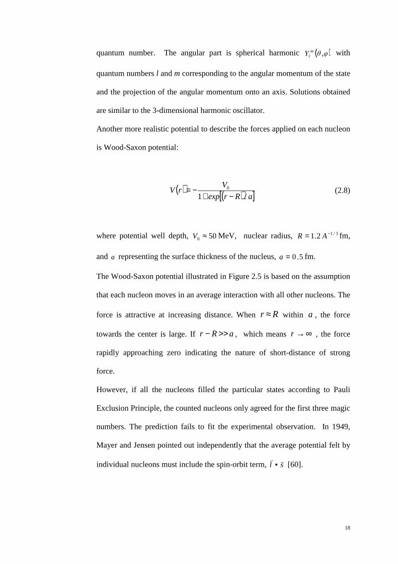
2.3.1 Vibration

“Phonons” of multipolarity λ is the vibrational quanta that carry energy. The

multipolarity λ is used to characterize the multipolarity of the nuclear surface.

One can imagine the nuclear vibration as a liquid drop vibrating at high

frequency. The nuclear average shape is spherical but the instantaneous shape

is not spherical as illustrated in Figure 2.8. The nucleus is assumed to perform

harmonic vibrations about the spherical shape [64].

The instantaneous coordinate ( )tR of a point on the nuclear surface at ( )φ,θ is

( ) ( )∑∑≥ −=

+=1λ

λ

λµ

λµλµav φ,θY)t(αRtR . (2.10)

Each spherical harmonic, ( )φ,θYλµ will have amplitude ( )tα λµ . Due to

reflection symmetry,

µλλµ αα −= .

23

Figure 2.8 A vibrating nucleus with spherical equilibrium shape [57].

The 0=λ (monopole) term corresponds to breathing mode of a compressible

fluid. The nuclear shape is spherical with average radius 310

/av ARR −= . The

typical dipole ( )1=λ mode corresponds to overall translation of center of mass

of the fluid. It occurs when the proton and neutron oscillate out of phase

against each other. This is a collective isovector ( )1=I mode. It has quantum

number −= 1πK (the parity of a phonon, π is given by ( )λ1− in even-even

nuclei and occurs at high energy. Low-energy quadrupole ( )2=λ vibrations

are dominant mode. This mode can have two forms in axially symmetric

deformed nucleus. Variation of nuclear modes of vibration is shown in Figure

2.9.

24

Figure 2.9 Modes of nuclear vibration [65].

The first, −β vibrations are the elongations along the symmetry axis. The

angular momentum vector of such shape oscillations is perpendicular to the

symmetry axis. Therefore, such bands are of += 0πK states. The second type

of vibration is −γ vibration which is the travelling wave with angular

momentum vector points along the symmetry axis. This gives rise to += 2πK

bands.

2.3.2 Deformation

Assume an incompressible deformed nucleus with constant volume, the

nuclear radius can be defined as the distance from the center of the nucleus to

the surface at angle ( )φ,θ and written as

25

( ) ( )

+= ∑∑

∞

= −=2

1λ

λ

λµ

λµλµav φ,θYαRφ,θR (2.11)

where λµα are the coefficients of the spherical harmonics ( )φ,θYλµ , the

average radius 310

/av ARR −= and 0R is the radius of spherical nucleus having

the same volume with the deformed nucleus. The value of λ determines the

type of multipole deformations and µ is the projection of λ on the symmetry

axis. The 2=λ terms represent the quadrupole deformations.

For pure quadrupole deformation,

( ) ( ) ( ) ( )[ ]φ,θYαφ,θYαφ,θYαRφ,θR av 2222222220201 −+++= . (2.12)

Lund convention expressed the coefficients as:

γcosβα 220 =

γsinβαα 22222 == −

with 2β is the eccentricity and γ is the non-axiality or degree of axiality.

Figure 2.10 summarizes the nuclear shapes variation in the ( )γ,β plane and

how they repeat every o60=γ . The plane is divided into six parts by

symmetries. In the 3-axis, the nucleus is in the prolate shape with one axis is

long, and the other two axes equal, i.e. conventionally yx= .

For spheroidal nuclei, the nuclear radius is

( ) ( )[ ]φ,θYβRφ,θR av 2021+= . (2.13)

The spheroidal nucleus has axial symmetry, either oblate (two equal semi-

major axes) o60=γ or prolate (two equal semi-minor axes) o0=γ . This

26

Figure 2.10 Nuclear shapes in the principal axes system as a function of γ for

fixed β [37].

nucleus is in ellipsoidal shape that is its cross section is ellipse. One symmetry

axis also is retained in this deformation. 2β is derived using the Lund’s

definition:

avR

R∆=53

42

πβ . (2.14)

R∆ is the difference between the semi-major and semi-minor axes of the

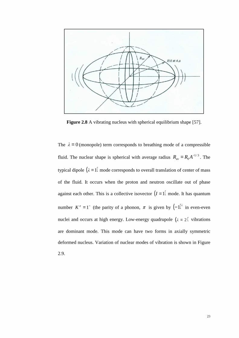
ellipsoid. Nuclear shapes variation in relation with eccentricity, 2β is

illustrated in Figure 2.11.

Nuclear charge distribution can be described by the effective shape of the

nucleus through a parameter called nuclear electric quadrupole moment, Q .

The value of electric quadrupole moment is related to its deformations by the

relation:

++= ...ββZRQ 2220 2

11

5

4. (2.15)

27

Figure 2.11 Nuclear shapes in relation with eccentricity, 2β [66].

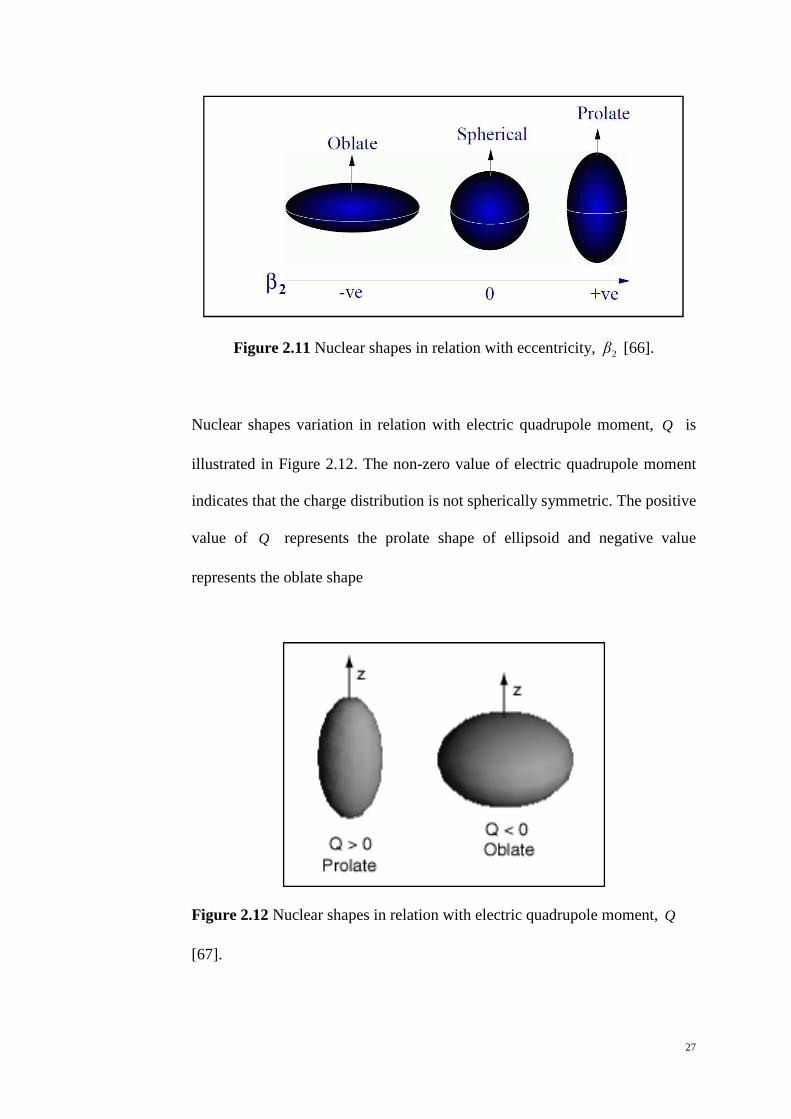
Nuclear shapes variation in relation with electric quadrupole moment, Q is

illustrated in Figure 2.12. The non-zero value of electric quadrupole moment

indicates that the charge distribution is not spherically symmetric. The positive

value of Q represents the prolate shape of ellipsoid and negative value

represents the oblate shape

Figure 2.12 Nuclear shapes in relation with electric quadrupole moment, Q

[67].

28

2.3.3 Axially Symmetric Ellipsoid Shape

Rotational motion can only be detected if the nucleus is in nonspherical shape.

The rotational of spherical nucleus is always on symmetry axis and the

orientation of the axes is indistinguishable quantum mechanically [68]. No

collective rotations occur about the symmetry axes. In axial-symmetric

deformed nucleus, the rotational symmetry is broken.

Imagine a deformed nucleus in a 3-dimensional ,(x ,y )z coordinate space

with its center of mass is at ,0( ,0 )0 coordinate. ( )y,x plane is the rotational

plane of the nucleus which perpendicular to z symmetry axis. By three

infinitesimal rotations, the ,(x )y plane is transformed into ,'( x )'y plane.

No rotation will be observed if the rotational axes are parallel to z axis. The

axially symmetric shape nuclei can only rotate along axes which are

perpendicular to symmetry axis. As no rotation about z axis, moment of

inertia about the other 'x and 'y axes are equal i.e. ℑ=ℑ=ℑ 'y'x [69]. Only

one value of ℑ is assigned for the rotational energy spectrum.

From Figure 2.13, the total angular momentum, Ir

can be expressed as:

JRIrrr

+=

where Rr

is the vector of rotational angular momentum, and Jr

is the angular

momentum vector of intrinsic motion, and has its component on z axis, K .

Quantum numbers are constants of motion. Angular momentum of intrinsic

motion j is not constant along with the rotation, so j cannot be considered

as good quantum number for deformed nuclei. For simplicity, the angular

29

Figure 2.13 Coupling scheme for particle in slowly rotating spheroidal

nucleus in 2-D coordinate system [70].

momentum of intrinsic motion is taken to be zero so that Rr

is the total

angular momentum:

RIrr

= .

The angular momentum of rotation Rr

is a constant of motion and is

perpendicular to the symmetry axis z for an axially symmetric nucleus (See

Figure 2.14). But, the quantum number K , the component of angular

momentum summation of individual valence nucleons, ∑=Ω j about the

symmetry axis has a fixed value for the rotational band [68].

If zR is the operator for the angular momentum along the symmetry axis, then

0ˆ =

∂Ψ∂−=Ψθ

hiRz . (2.16)

The axial-symmetric shape requires the Hamiltonian must be invariant with

30

Figure 2.14 The rotational angular momentum is not along the symmetry

axis and the intrinsic angular momentum is assumed to be zero, for

simplicity.

respect to rotations about the symmetry axis, so there is no associated

rotational energy about the symmetry axis. Only the phase is changing as the

consequence of the rotation about the symmetry axis.

The even parity wave function that fulfill the symmetry relation is

nonvanishing if

1)1( =− I .

Therefore the values for angular momentum are ,0=I ,2 ,4 ,6 ... or even

parity wave function. The linear superposition of the wave will cancel out for

odd I [60].

The degree of axial symmetry is zero with prolate shape.

31

2.3.4 Rotation Matrices

It is appropriate to introduce intrinsic (body-fixed) frame with )',','( zyx

coordinates and laboratory (space-fixed) frame with ,(x ,y )z coordinates.

Arbitrary rotation from ,(x ,y )z coordinates to )',','( zyx coordinates is

described by the familiar Euler angle, ,( 1θθ = ,2θ )3θ .

The following steps are done counterclockwise to arrive at the frame

)',','( zyx from the original frame ,(x ,y )z [65, 71]:

a) The system is rotated through an angle 1θ )πθ( 20 1 ≤≤ about z axis,

thereby changing the position of x and y axes. This yields

,( 1x ,1y )z .

b) The second rotation is through 2θ )πθ( 20 2 ≤≤ about the new

position of y axis. This yields ,( 2x ,1y )2z .

c) Finally, once again, rotation is done through 3θ )20( 3 πθ ≤≤ about

the newest position of z axis. This yields )',','( zyx where 2z'z = .

These three infinitesimal rotations through Euler angles

( ) ( )γ,β,αθ,θ,θθ == 321 are defined in Figure 2.15.

If we specify the relationship between the representations of state vector, the

rotated vector in the frame )',','( zyx is

IKIK ℜ=' (2.17)

where the rotation operator, )ˆexp( Ini r

h

•−=ℜ θ . We have to define respective

angular momentum operator for every infinitesimal rotation. Separating the

32

Figure 2.15 Rotation of the coordinate axes from ,(x ,y )z to )',','( zyx by

Euler angles ),,( γβα in three steps [41].

rotation operator to specify the ordered rotations through Euler angles,

)exp()exp()exp()()()( 123123 12 zyz Ii

Ii

Ii r

h

r

h

r

h

θθθθθθ −−−=ℜℜℜ=ℜ .

(2.18)

Fortunately,

)exp()exp()exp()exp( 1212 1 zyzy Ii

Ii

Ii

Ii r

h

r

h

r

h

r

h

θθθθ −−=− (2.19)

and

)exp()exp()exp( 123 12 zyz I

iI

iI

i r

h

r

h

r

h

θθθ −−=−

)exp()exp()exp(1213 yzz I

iI

iI

i r

h

r

h

r

h

θθθ−× . (2.20)

Finally, the full rotation in terms of angular momentum operator

)exp()exp()exp()( 321 zyz Ii

Ii

Ii r

h

r

h

r

h

θθθθ −−−=ℜ . (2.21)

33

Using closure of the set IM , we have the transformation of IK into

∑ ℜ=ℜ=M

IKIMIMIKIK ' . (2.22)

Figure 2.16 defines the relationship between the quantum numbers M and K

.

Figure 2.16 Relationship between the total angular momentum, Ir

, the

intrinsic angular momentum, Jr

, the rotational angular momentum, Rr

and the

component of Ir

along the rotational x axis, M and the symmetry axis in the

body-fixed frame, K [72].

Defining the rotation matrices, or the −D functions for short as the coefficient

of the relation

∑=M

IMKDIMIK )(' θ . (2.23)

IKIMD IMK )()( θθ ℜ= . (2.24)

IKIi

Ii

Ii

IMD zyzIMK )exp()exp()exp()( 321

r

h

r

h

r

h

θθθθ −−−= . (2.25)

34

Note that in Equation (2.21), the first and last operator is diagonal in the IK ,

and IM is an eigenfunction of zIr

. The matrix is simplified to

( ) IKIi

IMKMi

D yIMK )exp(exp)( 231

r

hh

θθθθ −

+−= . (2.26)

( ) )(exp)( 231 θθθθ IMK

IMK dKM

iD

+−=h

. (2.27)

)( 2θIMKd

is the real function of reduced rotation matrix:

IKIi

IMd yIMK )exp()( 22

r

h

θθ −= . (2.28)

[ ]∑ +−−+−−

−+−+−=s

sIMK sKMssKIsMI

KIKIMIMId

)!(!)!()!(

)!()!()!()!()1()(

2

1

2θ

KMssMKI −+−−+

−

×2

2

22

2

2sin

2cos

θθ. (2.29)

The summation is over all possible integer value of s for which the factorial

arguments are zero or greater.

The conjugate of )(θIMKD :

∑=M

IMK IMDIK )(' * θ . (2.30)

( ) )(exp)( 231* θθθθ I

MKIMK dKM

iD

+=h

. (2.31)

The IMKD matrices are unitary,

( ) '' * KKM

IMK

IMK DD δ=∑ and ( ) '' * MM

K

IMK

IKM DD δ=∑ .

It follows that

∑=K

IMK IKDIM ')(θ (2.32)

with the orthogonality relation between the −D functions,

35

( ) ( ) MKIKM

M

IMM

M

IMM

IKM DDDD δ==∑∑ ** '

''

'''

and

( ) '''

2'

''

2

0

2

0 03122 12

8*sin JJKKMM

IKM

IMK I

DDddd δδδπθθθθπ π π

+=∫ ∫ ∫ .

where the abδ is the Kronecker delta with value unity if ba = and zero

otherwise.

2.3.5 Rotational Excitations

If nucleus is deformed, the core and valence nucleons will rotate collectively.

The nonspherically symmetric potential is responsive to rotation because the

different orientation is distinguishable. The wave functions of the nucleons

that move collectively vary slowly with increasing angular momentum. For

collective rotation of even-even nuclei, in the symmetric case, only one

moment of inertia is defined leading to

ℑ=

2

2RH rot

r

. (2.33)

Quantum mechanically, ( )hv

1+= IIR for pure collective rotation [57, 68, 73,

74] that the total angular momentum, IRvv

= . Then the spectrum will take a

term that is consistent with the energy of rotational state. The rotational

excitation band is similar to

)1(2

2

+ℑ

= IITsymmtop

h

. (2.34)

In order of increasing excitation, the ground state band consists of

)1(2

2

+ℑ

= IIEI

h

with ,0=I ,2 ,...4 (2.35)

36

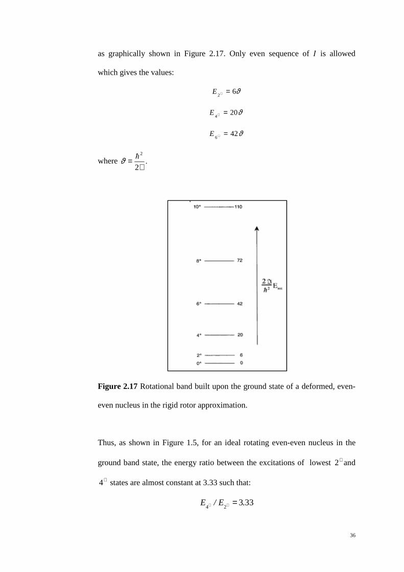
as graphically shown in Figure 2.17. Only even sequence of is allowed

which gives the values:

ϑ62

=+E

ϑ204

=+E

ϑ426

=+E

where .2

2

ℑ= hϑ

Figure 2.17 Rotational band built upon the ground state of a deformed, even-

even nucleus in the rigid rotor approximation.

Thus, as shown in Figure 1.5, for an ideal rotating even-even nucleus in the

ground band state, the energy ratio between the excitations of lowest +2 and

+4 states are almost constant at 3.33 such that:

33324

.E/E =++

37

directly indicates that the ideal rotating even-even nucleus is highly deformed

and located at the 190150 << A and 220<A mass region [39, 75]. This

constant ratio is for extreme rigid rotator. It can be used as rigidity indicator of

a nucleus. If a nucleus is subjected to centrifugal stretching, this ratio value

will take a smaller value.

The ground states of the even-even nuclei have += 0πK . The rotational

energy law is only valid for small value of I . The deviation from ( )1+II rule

is increasing with the increment of spinI . Figure 2.18 shows the abrupt

deviation of the ( )1+II rule as the spin I increases where the dotted straight

line is the predictions done by A. Bohr [76].

By analyzing Figure 1.3, the region of highly deformed, axially symmetric

rotational nuclei and the spherical vibrational nuclei can be specified. The

departure from the ( )1+II rule of certain nuclei indicates the transitional

regions between the highly deformed, axially symmetric rotational nuclei and

the spherical vibrational nuclei that are found slightly outside the region of

190150 << A and 220<A . The value 1202

=+E keV is closer to those of

axially symmetric rotators. On the other hand, the value the first +2 of level of

Sm150 is closer to those of single phonon vibrational energies of spherical

nuclei [71].

For a given A , increasing deformation affecting on the moment of inertia by

increasing it and lowering the excitation energy. This leads to smaller energy

spacing. Nucleus with larger A has the larger value of moment of inertia [75]

and smaller values of rotational energy. This is simply related to the

3

5

A=ℑ . (2.36)

38

Figure 2.18 Energy ratio in the ground band state in the even-even nuclei in

the 152 < A< 186. Data were taken from (Firestone et al. 1996) [76].

2.4 Nuclear Adiabatic Model (Unified Nuclear Model)

Nuclear adiabatic model is formulated by Bohr and Mottelson [41]. The model

is formulated as an attempt to unify the concepts of collective model and shell

model in the study of rotation-vibration interaction. The model states that the

lowest excited state of axially symmetric ellipsoid even-even nuclei is related

to rotational states with even angular momentum as a whole. The unified

model also states that the strong coupling of nucleonic motions to the rotor

and follow the rotational axis motion adiabatically.

39

The usual condition of adiabaticity is expressed as:

intωωω <<<< vibrot (2.37)

where rotω is the rotational angular frequency, vibω the vibrational angular

frequency, and intω the intrinsic angular frequency. This condition implies the

separation of rotational motions from the vibrations and single-particle

excitations. These three motions are treated independently.

The adiabatic approximation is valid if the rotational motion is sufficiently

slow without perturbing the nucleonic motion. Hence, the individual nucleon

can continuously readjust its wave function without changing states and

obliged to follow the deformations. The nucleus will change its shape in

smooth manner without sudden change on the intrinsic motion. Large number

of nucleons participates in the deformation [77].

In the unified nuclear model, the nuclear motion is expressed as three

independent modes; the intrinsic motion, vibrational motion, and the rotation

of the nucleus itself. Consequently, the Hamiltonian can be expressed as:

vibrotint HHHH ++= (2.38)

where intH is the Hamiltonian for the intrinsic motion, rotH the Hamiltonian

for the rotational motion, and vibH the vibrational Hamiltonian. For rigid

rotation, the rotational Hamiltonian is

( ) 222

2

1

2

1'z

'z'y'xrot RRRH

ℑ++

ℑ= (2.39)

where 'xR , 'yR and 'zR are the rotational angular momenta corresponding to

'x , 'y and 'z axes. Due to axial symmetry, 0='zR and moment of inertia

about the other 'x and 'y axes are equal i.e. ℑ=ℑ=ℑ 'y'x .

40

Using the equality from Figure 2.13:

JIRrrr

−=

where Rv

is the rotational angular momentum operator, decomposed into Iv

,

the total angular momentum operator which rotates the whole system and acts

only on the rotational wave function, and Jr

is the angular momentum

operator acting on intrinsic motion.

Now, the total Hamiltonian obtained is

vibcorrot HHTHH +++= int (2.40)

with

ℑ+=

2

)1(IITrot (2.41)

and

)(2

1+−−+ +

ℑ−= JIJIH cor . (2.42)

corH is referred to as the Coriolis coupling which is the coupling of intrinsic

and rotational motions. Coriolis interaction alters the projection of angular

momentum on the symmetry axis, admixing different values of K . K is only

a good quantum number when the potential is axially symmetry. ±I acts on

total angular momentum I , while ±J acts on intrinsic angular momentum j

. −+ JI decreases K and +− JI increases K . The nucleus is considered a

good rotational nucleus when the Coriolis effect is relatively small with small

reciprocal of moment of inertia ℑ2

1 , low angular momentum j , and low spin

I [78]. This term is neglected by the adiabatic approximation. But at high spin

41

I , a small axial asymmetry is produced and the adiabatic theory is deviated

[75].

2.4.1 Coriolis effect: Two states mixing

Mixing of two states is worth discussing in studying the effect of certain types

of mixing on transition rate. The concept of two-state mixing is used in

regards to its triviality and simple semi quantitative calculations without losing

the sight of the basic physics.

Consider two perturbed states 1ψ and 2ψ with approximately same energy,

spin and parity that can be written as combinations of pure wave functions

211 βφαφψ −=

212 αφβφψ +=

α and β are the normalization coefficients that represent the major and

minor components of the wave functions such that, βα > and 122 =+ βα .

The two levels repel each other by difference of ε (See Figure 2.19) and

change the moment of inertia.

Given the value of the perturbed (experimental) energies, 1expE and 2

expE , it is

possible to calculate the interaction matrix element xrot jω from the pure

energies 1theorE and 2

theorE , such that

=

2

12,1exp

2

12

1

φφ

φφ

ωω

EEj

jE

theorxrot

xrottheor . (2.43)

In general, the mixing depends both on the spacing of the initial unperturbed

energies between two states theorE∆ and on the strength of the matrix element

42

Figure 2.19 Two-level mixing.

xj [54, 75]. There are two limiting cases to be considered i.e. infinitely

strong and relatively weak mixing.

1. Suppose two initial states are degenerate. ( 0=∆ theorE ). The result is

that, for any isolated two-state system, the final separation can never

be closer than twice the mixing matrix element.

But, suppose two levels mix. They can never cross but repel and can

never be closer than twice the mixing matrix element after mixing.

This behavior acts as an indication of strong mixing.

2. The weak mixing limit corresponds to the large separation of the initial

unperturbed energies between two states relative to the mixing matrix

element ( 1>>∆ xtheor jE ).

The two-state mixing situation can be extended to define the description of

two different bands 1K and 2K mixing which is more complicated. The band

mixing can explain the back bending phenomenon [79].

43

2.5 Cranking Model

Rotational and vibrational motions are treated macroscopically in collective

model. Based on deformation symmetry and adiabaticity, the Coriolis

coupling does not appear explicitly, but manifests itself in low angular

momentum dependence [41]. In order to determine the collective variables and

parameters, microscopic modeling of both collective and single-particle

excitations is needed. To bring these two excitations to unity, cranking model

is added to deformed shell model. The effect of Coriolis coupling on the

Hamiltonian will be taken into account by adding the cranking term to the

quasiparticle energies. It is more practical to work in the intrinsic (body-fixed)

system than in the laboratory (space-fixed) system. Cranking model is suitable

to use as it can be extended to very high-spin states.

Cranking model as proposed by Inglis [80-81] is in semi classical context. The

nuclear excited states are characterized by the classical quantity which is the

angular momentum rather than the angular frequency. This model assumes

that independent nucleons in the ground state of a nucleus move within

deformed self-consistent many-particles potential react on external rotational

force applied onto them [69]. In short, moment of inertia is derived by rotating

the intrinsic wave. Further evaluation of the function can yield the energy

increment [74].

The coordinate system which is rigidly fixed to that potential rotates with

constant angular frequency ω . The angular frequency ω is conceived to be

smaller compared to that of the collective motion. Due to adiabaticity, the

intrinsic energies are larger than the rotational energies [73].

44

Considering a deformed potential well, U that is single-particle, self-

consistent, and fixed shape rotating about an axis in space [74, 82]. With

respect to rotational axis, spherical coordinate is introduced. At time 0=t ,

( ) ( )0;tωφ,θ,rUt;rU −=r . (2.44)

Nucleus is a dynamic system which depends on deformation variables and

time derivative. If the deformed potential well U depends on φ , U is time

dependence which means axial asymmetry is produced about rotational axis.

As we consider axially-symmetric deformed nuclei in this research, the time

dependence of the potential U will be eliminated later.

In laboratory system, we introduce time-dependent Hamiltonian H and a

state function ψ describing the motion that satisfies the Schrodinger equation:

ψi

ψH

∂∂= . (2.45)

The nucleus is assumed to rotate slowly about the x axis. This rotational x

axis is considerable to be perpendicular to the symmetry axis.

As mentioned before, the time dependence of the deformed potential U

needs to be eliminated to maintain axially symmetric condition. To eliminate

the time dependence, we can define unitary transformation, ( )tωiJexpU x−=

such that

( )φtUψ = (2.46)

whereϕ is the wave function in the latter system.

A transformation around rotational axis with angle, tωφ= is induced.

Replacing (2.46) into (2.45) yields:

45

( )( ) ( )( ) t/φtUiφtUH ∂∂=

( )( ) ( )t

φtU

t

φtUφi

∂∂+

∂∂= (2.47)

which rearranging the equation leads to:

t

φi

t

UφiφHUU

∂∂=

∂∂−−1 . (2.48)

Equation (2.48) may be rewritten as:

t/φiφH~ ∂∂= (2.49)

where is given by:

∂∂−= −

t

UiHUUH

~ 1 . (2.50)

Note that we define unitary transformation for simplicity,

( )tωiJexpU x−= (2.51)

and we can write H~

as follows:

( ) ( ) ( )[ ][ ] tωiJtωiJexpitωiJexpHtωiJexpH~

xxxx −−−−−=

= XJωH −0 . (2.52)

The so-called general many-body Hamiltonian of the cranking model consists

of two parts; the stationary state of the static Hamiltonian in the nuclear

system and the cranking term.

The cranking term is treated as perturbation if ω is small enough. If the

condition is fulfilled, the calculation of the quantity of the energy and function

can be done by means of perturbation theory. We can write:

φE~

φH~ = (2.53)

and the relation between the energy eigenvalues for the two systems with the

Coriolis interaction XJωr

r • is:

46

ψHψE = (2.54)

φJφωE~

X+= .

Inglis [72-73] developed the cranking formula for the moment of inertia:

∑ −><

=ℑik

ki

xinglis

kJi

εε

2||||2 (2.55)

where i and k are single particle bases and xJ is the rotational angular

momentum operator. Figure 2.20 shows the plotted moment of inertia in rare

earth nuclei.

Figure 2.20 Moments of inertia in rare earth nuclei [37].

2.6 Harris Parameterization

From the previous section, Inglis cranking formula [80-81] for the moment of

inertia is stated. But the cranking formula is the usual cranking model results

from the use of second-order perturbation theory. Harris parameterization [82]

47

included terms up to fourth order in X' JωH −= by making use of fourth-

order perturbation theory:

∑ −

>><<+=m mEE

HmmHEE

0

''

00||||0~

∑ −−−>><><><<+

mnp pnm EEEEEE

HppHnnHmmH

))()((

0||||||||0

000

''''

(2.56)

.|)()(

||0||||0| 2

20

20

'2'

∑−−

><><−mn mn EEEE

mHnH

Here, ϕ must be calculated to third-order perturbation theory for proper

normalization since terms up to fourth order is included in 'H :

∑ −

>><<−=m mEE

HmmHH

0

''' 0||||0

2|| ϕϕ

∑ −−−>><><><<−

mnp pnm EEEEEE

HppHnnHmmH

))()((

0||||||||04

000

''''

(2.57)

.)()(

|||0||||0|4

2

20

20

'2'

∑−−

><><+mn mn EEEE

mHnH

From (2.54), we obtain

∑ −>><<

−=m m

xx

EE

JmmJEE

0

20

0||||0ω

∑ −−−>><><><<

−mnp pnm

xxxx

EEEEEE

JppJnnJmmJ

))()((

0||||||||03

000

4ω

(2.58)

48

.)()(

|||0||||0|3

2

20

20

24∑

−−><><+

mn mn

xx

EEEE

mJnJω

Basically, the rotational energy is related to rotational frequency ω and all

terms containing the rotational frequency cannot be neglected. Expressed in

terms of rotational frequency, the expression of the energy of the laboratory

system is written in the form

20 2

1ω)ω(EE ℑ+= . (2.59)

We finally obtain the moment of inertia dependence on the angular frequency

expression:

( ) 20 3 ωCω +ℑ=ℑ (2.60)

where

∑ −><

=ℑm

m

x

EE

||J|m|

0

2

0

02 (2.61)

which is the expression that completely very similar to the usual cranking

formula obtained from the use of second-order perturbation treatment, and

∑ −−−>><><><<

=mnp pnm

xxxx

EEEEEE

JppJnnJmmJC

))()((

0||||||||02

000

.)(

|||0| 2

20

0∑ −><ℑ−

m m

x

EE

mJ (2.62)

The expectation value for the angular momentum of the intrinsic state ϕ is

( )20 2 ωCωφJφ x +ℑ= . (2.63)

49

Since higher-order perturbation theories are used, the rapid convergence of the

large correction terms in the perturbation series is often doubted. Self-

consistency approach is used to overcome the doubt.

From (2.59), we write the energy in the form

∑∞

=

+=0

220 2

1

p

ppωaωEE (2.64)

and from (2.63), the angular momentum is of the form as follows:

∑∞

=

=0

2

p

ppx ωbωφ|J|φ . (2.65)

From (2.54),

∑∞

=

+=0

22

p

ppωbωE

~E . (2.66)

Due to classical mechanics correlation,

0)~

)(( =−∂

∂IE rotrot

rot

ωωω

where ( )1+= III~ .

Expression (2.66) is differentiated to give

1222 +∑ ++∂∂=

∂∂ p

pp ω)p(b

ω

E~

ω

E . (2.67)

For a stationary solution of

( ) ( ) ( ) ( )ωφωE~

ωφωH~ =

applying a theorem due to Feynmann, one has

>∂∂=<

∂∂ ϕ

ωϕ

ω|

~|

~HE .

In this case,

50

><−=∂∂ ϕϕω

||~

xJE

∑∞

=

−=0

2

p

ppωbω (2.68)

Combining (2.67) and (2.68), we obtain

1212 +∑ +=∂∂ p

pp ω)p(b

ω

E . (2.69)

From (2.59), we get

12222

1 +∑ +=∂∂ p

pp ω)p(a

ω

E. (2.70)

By direct comparison, (2.69) and (2.70) are valid if )12()1( +=+ pbpa pp is

obeyed for allp . If we write

( )K++++ℑ+= 6420

20 753

2

1ωFωDωCωEE (2.71)

and

( )K++++ℑ= 6420 432 ωFωDωCωφJφ x , (2.72)

self-consistency is achieved.

If 0== FD , both equations agree with previous results. In, conclusion, the

rotational energy and angular momentum of deformed nuclei are

( )K++++ℑ= 6420

2 7532

1ωFωDωCωErot (2.71’)

and

( ) ( )K++++ℑ=+ 6420 4321 ωFωDωCωII . (2.72’)

51

CHAPTER 3

THE MODEL

Interesting properties of Sm,, 156154152 and Dy,,,,, 166164162160158156

isotopes as

deformed nuclei can be studied by applying the phenomenological model [52-

53]. The basic states to be considered in this model include the )K( π += 10

ground state band, 1β −= + )0( 2πK , 2β −= + )0( 3

πK , γ −= + )2( πK

vibrational bands and

+= νπ 1K collective states (ν is the number of

+1

collective states).

In order to explain the Coriolis mixing effect on the basis states of a nucleus

within the phenomenological model, we shall start the formulation of the

model with a stable deformed nucleus with a set of intrinsic axes connected to

the rotation of laboratory axes by Euler angles, θ . We begin by introducing

the nuclear Hamiltonian containing rotational part ( )2IH rot and the Coriolis

interaction dependence part:

( ) ( )IHIHH σ

K,Krot += 2 . (3.1)

The Coriolis interaction dependence part of the Hamiltonian is

1,,,, '''' ),())(()( ±−−= KKKKxrotKKKKK KIjIIH δχωδωσ . (3.2)

In Equation (3.2),

',)( KKxj is the matrix element describing the Coriolis

coupling of rotational bands, )(Irotω is the angular frequency of core rotation,

yielded from

dI

IdEI rot

rot

)()( =ω (3.3)

52

(note that, for convenience, we have removed the factor h from each angular

momentum operator throughout this thesis.), and Kω is the band head energy

of respective theπK bands which is the lowest energy level and

,(Iχ ,1)0 = ,(Iχ .)1(

21)1

2

1

+−=

II (3.4)

The Kronecker delta , 1', =KKδ if 'KK = or 0', =KKδ if otherwise.

It is well established that a nucleus contains strongly interacting Fermi

particles that obey the Pauli Exclusion Principle. Fermions must have anti-

symmetric wave functions under the interchange of particles. The wave

function of the nuclear Hamiltonian

IMKK

IKK

IMK ∑=

''ψφ

[ ] 011

216

12

0

02

−++

++= ∑ +−−

++

'KK

IK,M

KI'K

I'K,M

,'K

IK,'KI

,MI

K,gr 'b)θ(D)(b)θ(Dδ

ψDψ

π

I

. (3.5)

IKK ,'ψ

are the amplitudes of basis states mixing from the )4( ν+ bands

includes the )0( 1+=πK ground state band,

and the single-phonon

00,2++

= = KK bbλ with 1β −= + )0( 2

πK , 2β −= + )0( 3πK , γ −= + )2( πK

vibrational bands and

+= νπ 1K collective states (ν is the number of

+1

collective states). The 0,'1 Kδ+ factor in the second term takes into account the

difference in the normalization between ,02+=πK +

30 and += 2πK bands.

By solving the Schrödinger equation

IqKq

IqKqKH ,,, ' ψεψ σσ = (3.6)

53

one obtains wave function and energy of states with positive parity.

The total energy of states is taken to be

)()()( IIEIE qrotqσσ ε+= . (3.7)

There are different methods available to determine the energy of rotational

core )(IErot . Harris parameterization of the angular momentum and energy

[82] is chosen to determine the energy of rotational core )(IErot :

( ) ( ) ( )IωIωIE rotrotrot4

12

0 4

3

2

1 ℑ+ℑ= (3.8)

( ) ( ) ( )IωIωII rotrot3

101 ℑ+ℑ=+ (3.9)

where 0ℑ and 1ℑ are the adjustable inertial parameters of rotational core. A

method of defining the even-even deformed nuclei inertial parameters using

the experimental data up to h8≤I for ground band is suggested in [83].

By solving the cubic equation, we obtain the rotational frequency of the core

( )Irotω . The resulting real root is as follows:

( )3

1

2

13

1

0

2

11

3

1

2

13

1

0

2

11 322322

ℑℑ

+

ℑ−

ℑ+

ℑℑ

+

ℑ+

ℑ= I

~I~

I~

I~

Iωrot

(3.10)

where )1(~ += III . Equation (3.10) gives value of ( )Iωrot at the given spin

I.

3.1 Determination of )I(ωrot

In the cranking model, ( )Iωrot is the rotational angular frequency which is

determined by imposing that the ( )1~ +== IIIJ x

54

The inter-dependency of I and 2rotω is introduced by Harris [82]:

( ) ( ) ( )IωIωIE rotrotrot4

12

4

3

2

1 ℑ+ℑ= 0 (3.11)

( ) ( ) ( )IωIωII rotrot3

101 ℑ+ℑ=+ . (3.12)

Rearranging the expression:

( ) ( ) I~

IωIω rotrot =ℑ+ℑ 310

( ) ( ) 0310 =−ℑ+ℑ I

~IωIω rotrot

( ) ( ) 011

03 =ℑ

−ℑℑ

+ I~

IωIω rotrot .

By supposing q=ℑℑ 10 , rI~ =ℑ− 1 and setting ( ) ωIωrot = to construct a

simple new cubic equation which is

03 =++ rqωω . (3.13)

It is appropriate to replace z+=νω into the simple cubic equation which

gives

.0 33 3223 =++++++ rqzqzzz νννν (3.14)

It is clear that Equation (3.14) is separable into two parts which if added

together will equal to zero.

033 22 =+++ qzqz z ννν (3.14a)

and

.rzν 033 =++ (3.14b)

By factorization of (3.14a),

( )( ) .03 =++ zqz νν

We note that either qz +ν3 or z+ν might equal to zero. But obviously we

can say that 0≠+ zν because z+=νω cannot be zero.

55

Here, we have two coupled equations: (3.14b) and

0.qz ν =+3 (3.13c)

Then, we have from (3.14c)

3

q-z =ν

and later becomes

.qzν 27333 −= (3.15)

Straightforwardly, we find from (3.14b)

.33 rz −=+ν (3.16)

The use of sum and product rules is a very convenient way to reduce the cubic

equations to much simpler form of quadratic equation:

( ) 033332 =++− zvxzvx (3.17)

( ) ( ) 02732 =−+−− qxrx (3.17a)

such that 3ν=x or 3zx = .

From the general solution of quadratic equation, the solutions are

( )2

274 32 qrrx

−±−=

32

3

1

2

12

+

±−= qrrx (3.18)

3

1

2

132

3

1

2

1

2

+

+−= qrrν (3.19)

56

3

1

2

132

3

1

2

1

2

+

−−= qrr

z (3.20)

Recall that z+=νω and ( )Irotωω = which yield

( ) .3

1

2

1

23

1

2

1

2

3

1

2

1

323

1

2

1

32

+

−−+

+

+−= qrr

qrr

Irotω

(3.21)

Finally, we replace 10 ℑℑ=q , 1

~ ℑ−= Ir in above expression, the rotational

frequency of the core ( )Irotω is now given by

( )3

1

2

13

1

0

2

11

3

1

2

13

1

0

2

11 32

~

2

~

32

~

2

~

ℑℑ

+

ℑ−

ℑ+

ℑℑ

+

ℑ+

ℑ= IIII

Irotω .

(3.22)

3.2 Determination of 0ℑ and 1ℑ

The ground states of the even-even nuclei have += 0πK . The necessary

condition for the rotational energy law to be valid is small value of I . The

deviation from )1( +II rule is increasing with the increment of spin I .

Rotational angular frequency for the nucleus is:

2

11 )I(E)I(E)I(ω

expexp

eff−−+= (3.23)

where )(exp IE is the energy from experiment [6-15].

57

Effective moment of inertia )I(effℑ is written in terms of nuclear rotational

angular frequency )I(ωeff :

)I(ω

)I(I)I(

effeff

1+=ℑ . (3.24)

Evaluating the above expression, one obtains the effective moment of inertia

for states )I(effℑ .

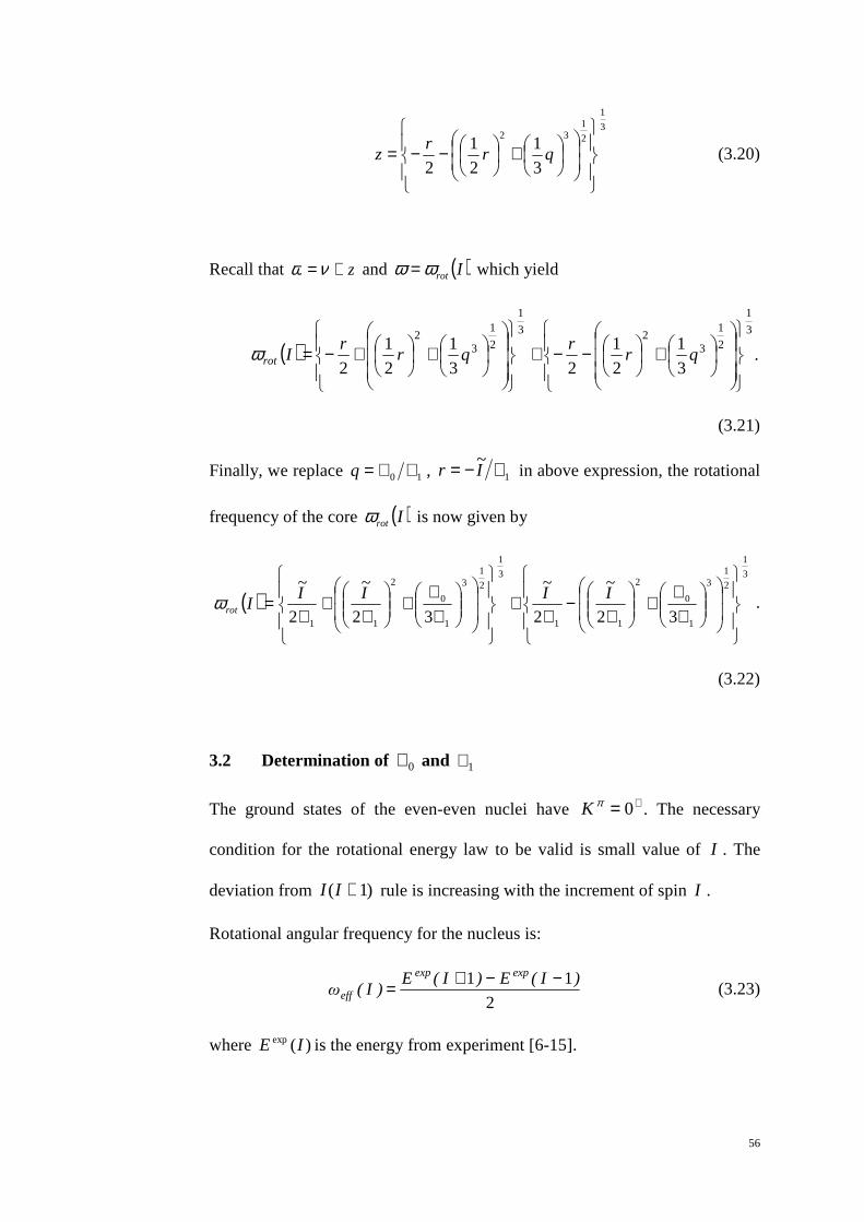
If we plot )I(effℑ as a function of )I(ωeff2 at low spin h8≤I , the relation is

verified to be mainly linear. This relation of the parameters is rephrased by

using Harris two-parameter formula:

)I(ω)I( effeff2

10 ℑ+ℑ=ℑ . (3.25)

Equation (3.25) defines the inertia parameters 0ℑ and 1ℑ for the effective

moment of inertia )(Ieffℑ when h8≤I . The effective moment of inertia

depends on the degree of rotation. The least square method is used in the

equation to determine the numerical values of the parameters 0ℑ and 1ℑ .

The inertial parameters, 0ℑ and 1ℑ have their interesting physical meanings.

The parameter 0ℑ is the moment of inertia of the ground states band and the

parameter 1ℑ represents the rigidity of the nucleus that leads to the centrifugal

stretching effect [83-84].

3.3 Determination of ( ) ',KKxj

The lowest energies for ground-state and −nβ bands were taken from

experimental energies, since they are not affected by the Coriolis forces at spin

0=I :

58

)0(exptgrgr E=ω

and )0(expt

nnEββω = .

The band head energies for the collective +1 states in Sm156,154,152 and

Dy166,164,158,156 nuclei are assumed to be 31 =ω MeV because the +=1πK

bands have not been observed experimentally for these nuclei respectively

[53]. Coriolis rotational states mixing matrix elements ',)(

KKxj and −γ band

head energies γω are determined by using the least square fitting method of

the diagonalize matrix

=

−−

+ 2

1

2

1

1 φφ

ωφφ

εωωωεω

Kxrot

xrotK

j

j.

Currently, the experimental energy spectrum for the +2

0β band in the Sm156

and Dy166 nuclei are not available. No calculations are done for this band in

respective nuclei.

59

CHAPTER 4

RESULTS AND DISCUSSIONS

The values of the inertial parameters, 0ℑ and 1ℑ are obtained from Equation

(3.25). )(Ieffℑ is plotted as a function of )(2 Ieffω at low spin, h8≤I . The linear

dependency of effective moment of inertia )(Ieffℑ on the square of angular

frequency )(2 Ieffω is invalidating at higher spin. Figures 4.1-4.3 illustrate the

linear dependency of )(Ieffℑ on )(2 Ieffω at low spin, h8≤I for isotopes

Sm,, 156154152 . Figures 4.7-4.12 show the same behavior of the relation for isotopes

Dy,,,,, 166164162160158156 . By using Equations (3.23) – (3.25) and utilizing least square

method, 0ℑ and 1ℑ are deduced from the fitted straight lines. The values of the

inertial parameters, 0ℑ and 1ℑ obtained are tabulated in Table 4.1 for isotopes

Sm,, 156154152 and Table 4.6 for isotopes Dy,,,,, 166164162160158156 .

From Tables 4.1 and 4.6, within same number of protons, for constant total

angular momentum i.e. for ground band state, the moment of inertia increases

gradually with nuclear size. This case is subjected to conservation law. To

conserve the total angular momentum while the nuclear size increases, the nuclear

moment of inertia must increase and the rotation of the nucleus must slow down.

The centrifugal stretching will come into play by decreasing the nucleons pairing

correlation and the nucleus fails to preserve its spherical shape. Thus, larger

nucleus lacks more in rigidity and is more deformed. The smallest values of 1ℑ

occur when the deformed prolate minimum in the potential energy surface.

60

It is generally known that the effective moment of inertia of the ground-state band

is smaller compared to that of nβ −++ )0,0(21 ββ and −γ bands, ),( γβ ℑℑ<ℑ

ngr.

This arises because the Coriolis mixing of these bands with += ν

πK 1 rotational

bands is more intense than the mixing of ground band state with += νπ 1K bands.

The effect of += νπ 1K bands on low-lying levels is interesting to study. The

intensity of mixing can be analyzed from the values of Coriolis interaction matrix

elements, ( ) 'K,Kxj and band head energy, Kω .

Wave function of states IMKφ represents the mixture components of other bands in

certain band. Tables 4.3-4.5 give the calculated wave function of states IMKφ for

Sm,, 156154152 and Tables 4.8-4.13 give the calculated wave function of states IMKφ

for Dy,,,,, 166164162160158156 . The wave function of states IMKφ is obtained by solving

the nuclear Hamiltonian in the form of Equation (3.2) by using the wave function

of Equation (3.5). Structure of Sm,, 156154152 and Dy,,,,, 166164162160158156 can be

understood by these calculated values.

The results are presented as simple two-state mixing form because of triviality.

The most important thing to understand are the relationships between the pure

band head energies spacings 'K,Kω∆ and the value of Coriolis mixing matrix

elements ( ) 1,Kxj , on one hand, the perturbed energy separations and the admixed

wave functions on the other hand. In general, the mixing depends both on the

proximity of the band head energy Kω between two bands and on the matrix

element 1,)( Kxj [54, 75].

61

The actual nuclear states are complex admixtures of many components. The

strong mixing of respective intrinsic excitation states will lead to the

nonadiabaticity of electromagnetic transition from +1

0β , +2

0β and γ state bands

[50-52]. This is an attempt to present accurate treatment to show the realistic

calculation of nuclear spectra. Rotational motion can be superimposed on the

vibrational motions. The rotational and intrinsic motions are strongly coupled due

to Coriolis forces. The non-adiabatic effects become more important as the

rotational frequency increases. The adiabatic assumption is applied on the wave

function of Equation (3.5) to separate the rotational and intrinsic motions.

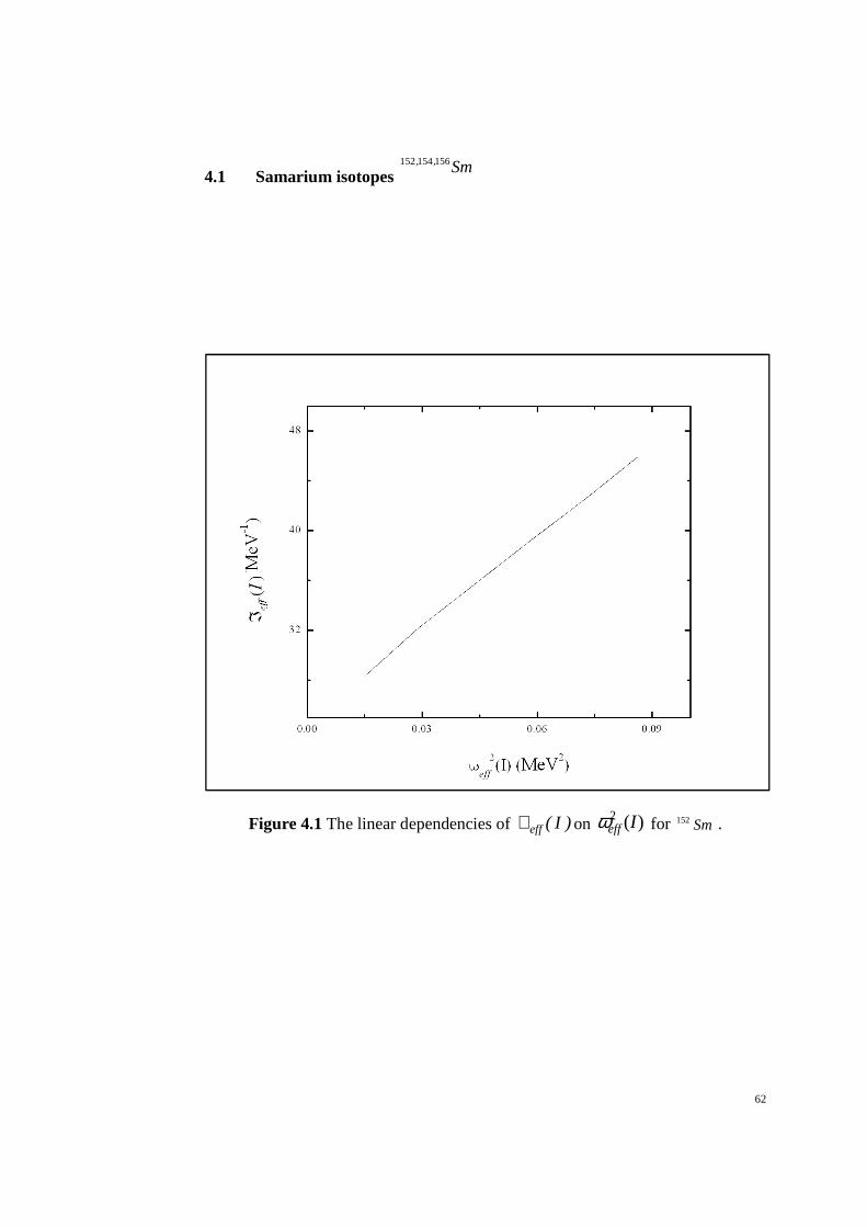
62

4.1 Samarium isotopes Sm,, 156154152

Figure 4.1 The linear dependencies of )I(effℑ on )(2 Ieffω for Sm152 .

63

Figure 4.2 The linear dependencies of )I(effℑ on )(2 Ieffω for Sm154 .

64

Figure 4.3 The linear dependencies of )I(effℑ on )(2 Ieffω for Sm156 .

65

Table 4.1 Inertial parameters of rotational core used in the calculations.

Nucleus 0ℑ (MeV-1) 1ℑ (MeV-3)

Sm152 24.74 256.57

Sm154 36.07 178.88

Sm156 39.22 98.36

Table 4.2 Parameters used in the calculations. Band head energies in MeV [6].

Nucleus 1βω

2βω 1ω γω 1,)( grxj 1,1

)( βxj 1,2)( βxj 1,)( γxj

Sm152 0.685 1.083 3.0 1.0 0.742 0.821 0.864 0.855 Sm154 1.099 1.203 3.0 1.380 0.345 0.403 0.408 0.417 Sm156 1.068 - 3.0 1.365 0.749 0.872 - 0.903

66

Table 4.3 Structure of Sm152 states.

I

gr

+1

0β +

20β +1

γ gr

+

10β

+2

0β +1 γ

Ground-state band +

10β

2 -0.9997 -

0.0025 -0.0016 -0.0227 -0.0014 0.0032 -0.9994 -0.0064 -0.0326 -0.0065

4 -0.9993 -

0.0065 -0.0043 -0.037 -0.0044 0.0086 -0.9982 -0.0169 -0.0536 -0.0199

6 -0.9987 -

0.0109 -0.0073 -0.0483 -0.0076 0.0148 -0.9964 -0.0283 -0.0704 -0.0343

8 -0.9981 -

0.0153 -0.0103 -0.0576 -0.0108 0.0211 -0.9942 -0.0397 -0.0845 -0.0485

10 -0.9975 -

0.0197 -0.0132 -0.0657 -0.014 0.0275 -0.9917 -0.0508 -0.0968 -0.0621

12 -0.9968 -

0.0239 -0.016 -0.0729 -0.017 0.0338 -0.9888 -0.0615 -0.1078 -0.0752

γ +

20β

2 0.0022 0.0078 -0.0302 -0.0326 -0.9990 -0.0025 -0.0075 0.9987 0.0395 -0.0316

3 - - - 0.0473 0.9989 - - - - -

4 -0.0069 -0.0248 0.0888 0.0630 0.9937 -0.006 -0.0182 0.9938 0.0585 -0.093

5 - - - 0.0698 0.9976 - - - - -

6 -0.0122 -0.0442 0.1452 0.0853 0.9846 -0.009 -0.0277 0.9855 0.0686 -0.1526

7 - - - 0.0866 0.9962 - - - - -

8 0.0175 0.0643 -0.1942 -0.1028 -0.9733 0.0115 0.0355 -0.9753 -0.0736 0.2049

9 - - - 0.1000 0.9950 - - - - -

10 -0.0226 -0.0843 0.2352 0.1168 0.9610 -0.0134 -0.0416 0.9645 0.0759 -0.2492

11 - - - 0.1112 0.9938 - - - - -

12 -0.0274 -0.1038 0.2691 0.1282 0.9485 -0.0149 -0.0464 0.9538 0.0766 -0.2865

67

Table 4.4 Structure of Sm154 states.

I

gr +

10β

+2

0β +1 γ gr

+1

0β +

20β +1

γ

Ground-state band +

10β

2 1.0 0.0002 0.0002 0.0076 0.0001 0.0003 -

0.9999 -

0.0037 -

0.0142 -

0.0011

4 -

0.9999 -

0.0006 -

0.0005 -

0.0134 -

0.0004 0.0009

-0.9996

-0.0114

-0.0250

-0.0041

6 0.9998 0.0011 0.0010 0.0184 0.0009 0.0017 -

0.9991 -

0.0215 -

0.0347 -

0.0080

8 0.9997 0.0016 0.0015 0.0228 0.0013 -

0.0027 0.9984 0.0329 0.0435 0.0124

10 0.9996 0.0022 0.0021 0.0266 0.0018 -

0.0037 0.9975 0.0449 0.0515 0.0172

12 0.9995 0.0029 0.0026 0.0301 0.0023 -

0.0048 0.9964 0.0571 0.0589 0.0221

+

20β γ

2 0.0003 0.0039 -

0.9999 -

0.0151 -

0.0019 -

0.0002 -

0.0013 -

0.0021 0.0139 0.9999

3 - - - - - - - - 0.0216 0.9998

4 -

0.0009 -

0.0121 0.9996 0.0262 0.0067

-0.0008

-0.0047

-0.0075

0.0280 0.9996

5 - - - - - - - - 0.0344 0.9994

6 -

0.0016 -

0.0228 0.9990 0.0358 0.0129

-0.0016

-0.009 -

0.0145 0.0390 0.9991

7 - - - - - - - - 0.0451 0.9990

8 0.0025 0.035 -

0.9982 -

0.0439 -

0.0197 -

0.0024 -

0.0138 -

0.0223 0.0480 0.9985

9 - - - - - - - - 0.0543 0.9985

10 0.0034 0.048 -

0.9972 -

0.0508 -

0.0265 -

0.0032 -

0.0187 -

0.0303 0.0554 0.9978

11 - - - - - - - - 0.0623 0.9981

12 0.0042 0.0612 -

0.9959 -

0.0568 -

0.0333 -

0.0040 -

0.0236 -

0.0383 0.0617 0.9971

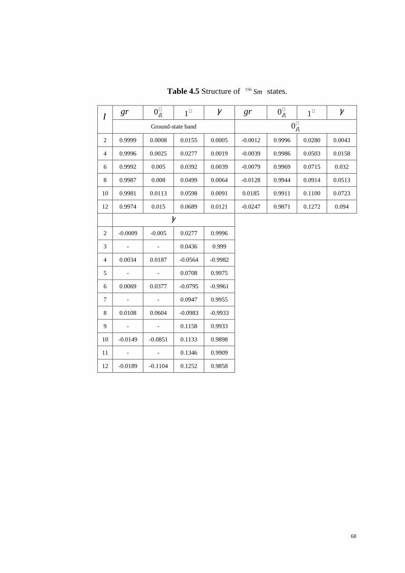
68

Table 4.5 Structure of Sm156 states.

I

gr +

10β +1

γ gr +

10β +1

γ

Ground-state band +

10β

2 0.9999 0.0008 0.0155 0.0005 -0.0012 0.9996 0.0280 0.0043

4 0.9996 0.0025 0.0277 0.0019 -0.0039 0.9986 0.0503 0.0158

6 0.9992 0.005 0.0392 0.0039 -0.0079 0.9969 0.0715 0.032

8 0.9987 0.008 0.0499 0.0064 -0.0128 0.9944 0.0914 0.0513

10 0.9981 0.0113 0.0598 0.0091 0.0185 0.9911 0.1100 0.0723

12 0.9974 0.015 0.0689 0.0121 -0.0247 0.9871 0.1272 0.094

γ

2 -0.0009 -0.005 0.0277 0.9996

3 - - 0.0436 0.999

4 0.0034 0.0187 -0.0564 -0.9982

5 - - 0.0708 0.9975

6 0.0069 0.0377 -0.0795 -0.9961

7 - - 0.0947 0.9955

8 0.0108 0.0604 -0.0983 -0.9933

9 - - 0.1158 0.9933

10 -0.0149 -0.0851 0.1133 0.9898

11 - - 0.1346 0.9909

12 -0.0189 -0.1104 0.1252 0.9858

69

For Sm152 , the Coriolis mixing matrix elements 864.0)( 1,2=βxj MeV-1 and

855.0)( 1, =γxj MeV-1 are considered to be larger values from others. These

two comparably equal and large values Coriolis mixing matrix elements, with

very small band head energies spacings 083.0,2=∆ γβω MeV induced strong

mixing between −+2

0β and −γ bands.

A large spacing of the band head energies between two bands reduces the

influence of large mixing matrix element. One nice example occurs in the

structure of Sm154 . Coriolis mixing matrix element 417.0)( 1, =γxj MeV-1

which is the highest among others and the pure band head energies spacings

17702

.ω β,γ =∆ MeV, 28101

.ω β,γ =∆ MeV, and 3801.ω γ,gr =∆ MeV. Even

though the mixing matrix element is large; the large spacing reduces its effect.

The strong mixing induced in this isotope is between −+1

0β and −+2

0β bands

with Coriolis mixing matrix elements 408.0)( 1,2=βxj MeV-1 and

403.0)( 1,1=βxj MeV-1. The Coriolis mixing between these bands is

strengthened by the small band head energy spacings, 104.012 , =∆ ββω MeV.

The experimental energies for −+2

0β band in Sm156 isotope are not available.

No calculations are done for this band. Insufficient number of states from

other rotational bands and unavailability of −+2

0β band make it difficult to

explain the structure of Sm156 isotope by comparison. The intensity of

Coriolis mixing between −+1

0β and −γ bands is noticeable. This is because

the Coriolis mixing matrix elements 903.0)( 1, =γxj MeV-1 is the highest

followed by 872.0)( 1,1=βxj MeV-1 and 749.0)( 1, =grxj MeV-1. The Coriolis

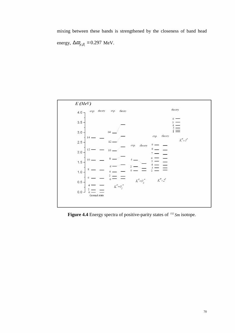
70

mixing between these bands is strengthened by the closeness of band head

energy, 297.01, =∆ βγω MeV.

Figure 4.4 Energy spectra of positive-parity states of Sm152 isotope.

71

Figure 4.5 Energy spectra of positive-parity states of Sm154 isotope.

72

Figure 4.6 Energy spectra of positive-parity states of Sm156 isotope.

73

The theoretical energy spectra of positive-parity states in Sm,, 156154152 are

presented in Figures 4.4, 4.5 and 4.6 respectively in comparison with the

experimental energies [6-9]. The theoretical energy spectra are calculated by

using Equation (3.7). From the figures, we see that energy difference

)I(E)I(E)I(ε exptheor −= of the −+1

0β band increases with the increase in

the angular momentum I. At high spin, I the nonadiabaticity of energy

rotational bands occurs. Two states with same spin, I and parity, π from

different bands cross in that region causes Coriolis mixing. We predict the

existence of s-band states to perturb the pure −+1

0β band states.

Other than this mentioned obvious deviation, the theoretical positive-parity

states energy spectra are in best agreement with the experimental data. But at

higher spin, I the theoretical energies deviate from the observed energies

suggests the nonadiabaticity of energy rotational bands. Few new states and

collective +1 band are predicted.

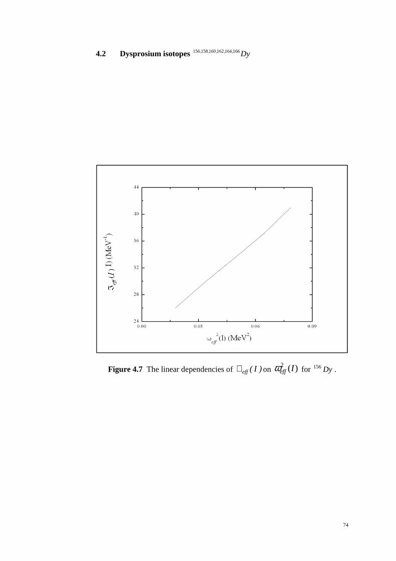
74

4.2 Dysprosium isotopes Dy,,,,, 166164162160158156

Figure 4.7 The linear dependencies of )I(effℑ on )(2 Ieffω for Dy156 .

75

Figure 4.8 The linear dependencies of )I(effℑ on )(2 Ieffω for Dy158 .

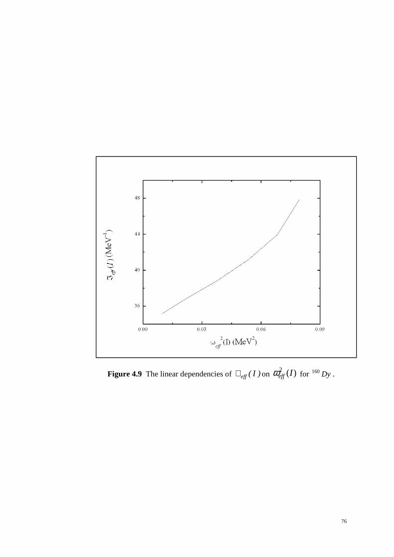
76

Figure 4.9 The linear dependencies of )I(effℑ on )(2 Ieffω for Dy160 .

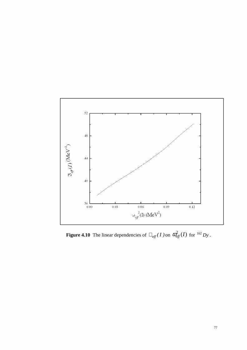
77

Figure 4.10 The linear dependencies of )I(effℑ on )(2 Ieffω for Dy162 .

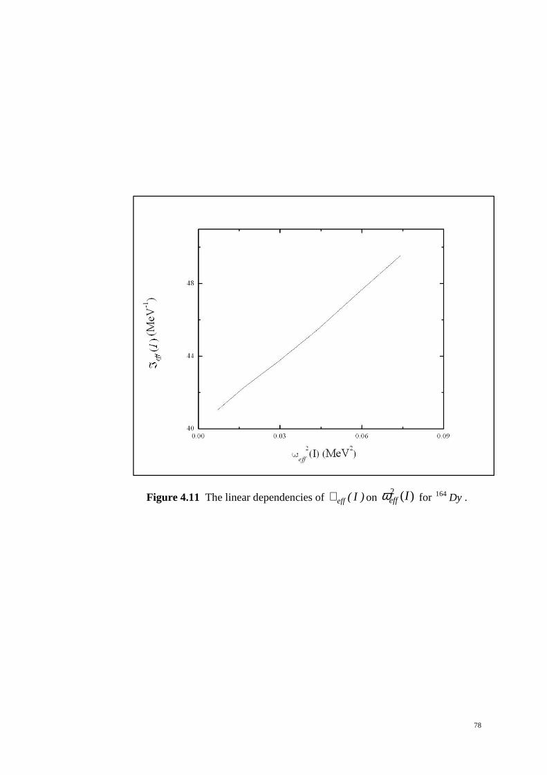
78

Figure 4.11 The linear dependencies of )I(effℑ on )(2 Ieffω for Dy164 .

79

Figure 4.12 The linear dependencies of )I(effℑ on )(2 Ieffω for Dy166 .

80

Table 4.6 Inertial parameters of rotational core used in the calculations.

Nucleus 0ℑ (MeV-1) 1ℑ (MeV-3)

Dy156 21.93 238.13

Dy158 29.69 174.26

Dy160 33.96 131.07

Dy162 36.61 105.77

Dy164 40.25 121.09

Dy166 38.68 73.81

Table 4.7 Parameters used in the calculations. Band head energies in MeV [6].

Nucleus 1βω

2βω 1ω γω 1,)( grxj 1,1

)( βxj 1,2)( βxj 1,)( γxj

Dy156 0.676 1.405 3.0 0.760 1.462 1.615 1.765 1.633

Dy158 0.991 1.269 3.0 0.847 2.598 2.966 2.605 2.481

Dy160 1.280 1.444 1.775 0.879 1.689 2.170 2.224 2.031

Dy162 1.400 1.666 1.720 0.807 0.077 0.103 0.108 0.093

Dy164 1.655 1.773 3.0 0.688 0.389 0.484 0.490 0.431

Dy166 1.149 - 3.0 0.780 0.174 0.205 - 0.195

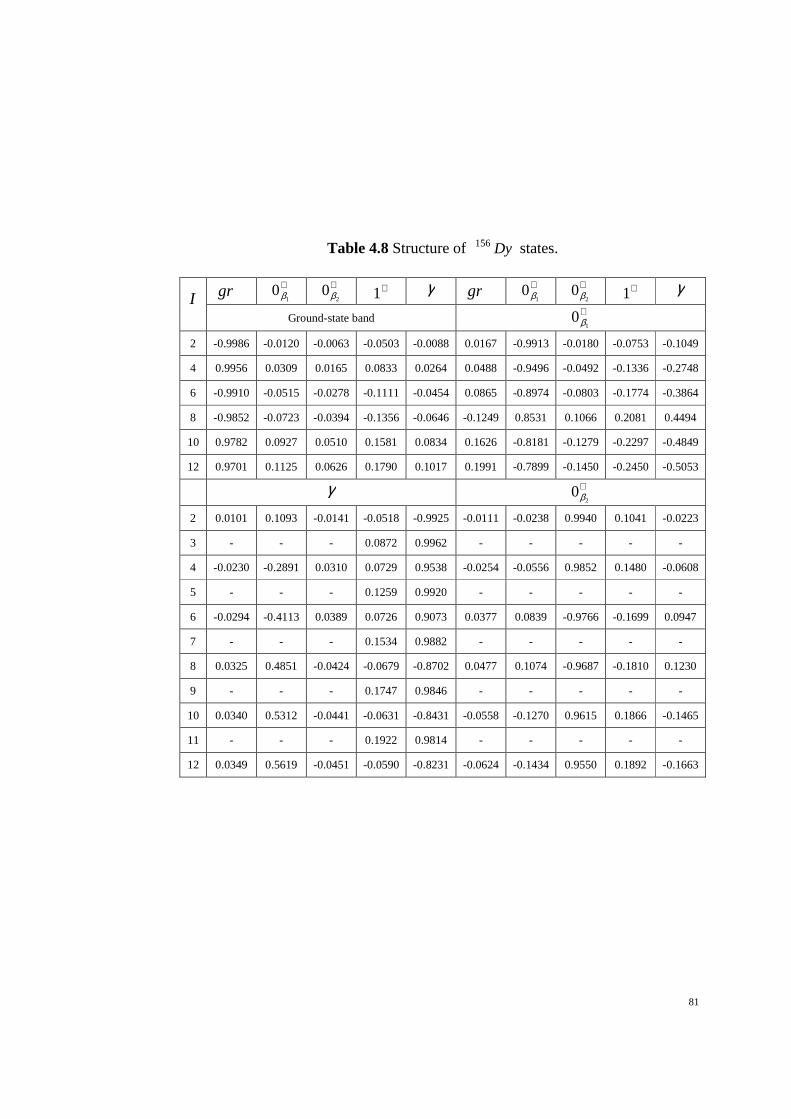
81

Table 4.8 Structure of Dy156 states.

I

gr

+1

0β +

20β +1

γ gr

+

10β

+2

0β +1 γ

Ground-state band +

10β

2 -0.9986 -0.0120 -0.0063 -0.0503 -0.0088 0.0167 -0.9913 -0.0180 -0.0753 -0.1049

4 0.9956 0.0309 0.0165 0.0833 0.0264 0.0488 -0.9496 -0.0492 -0.1336 -0.2748

6 -0.9910 -0.0515 -0.0278 -0.1111 -0.0454 0.0865 -0.8974 -0.0803 -0.1774 -0.3864

8 -0.9852 -0.0723 -0.0394 -0.1356 -0.0646 -0.1249 0.8531 0.1066 0.2081 0.4494

10 0.9782 0.0927 0.0510 0.1581 0.0834 0.1626 -0.8181 -0.1279 -0.2297 -0.4849

12 0.9701 0.1125 0.0626 0.1790 0.1017 0.1991 -0.7899 -0.1450 -0.2450 -0.5053

γ +

20β

2 0.0101 0.1093 -0.0141 -0.0518 -0.9925 -0.0111 -0.0238 0.9940 0.1041 -0.0223

3 - - - 0.0872 0.9962 - - - - -

4 -0.0230 -0.2891 0.0310 0.0729 0.9538 -0.0254 -0.0556 0.9852 0.1480 -0.0608

5 - - - 0.1259 0.9920 - - - - -

6 -0.0294 -0.4113 0.0389 0.0726 0.9073 0.0377 0.0839 -0.9766 -0.1699 0.0947

7 - - - 0.1534 0.9882 - - - - -

8 0.0325 0.4851 -0.0424 -0.0679 -0.8702 0.0477 0.1074 -0.9687 -0.1810 0.1230

9 - - - 0.1747 0.9846 - - - - -

10 0.0340 0.5312 -0.0441 -0.0631 -0.8431 -0.0558 -0.1270 0.9615 0.1866 -0.1465

11 - - - 0.1922 0.9814 - - - - -

12 0.0349 0.5619 -0.0451 -0.0590 -0.8231 -0.0624 -0.1434 0.9550 0.1892 -0.1663

82

Table 4.9 Structure of Dy158 states.

I

gr

+1

0β +

20β +1

γ gr

+

10β

+2

0β +1 γ

Ground-state band +

10β

2 0.9972 0.0167 0.0115 0.0712 0.0133 -0.0230 0.9804 0.0730 0.1071 -0.1466

4 -0.9885 -0.0506 -0.0350 -0.1302 -0.0466 -0.0452 0.8839 0.1274 0.1199 -0.4314

6 -0.9713 -0.0942 -0.0658 -0.1883 -0.0886 0.0514 -0.7887 -0.1368 -0.0999 0.5888

8 -0.9453 -0.1406 -0.0992 -0.2434 -0.1327 0.0525 -0.7336 -0.1364 -0.0834 0.6584

10 -0.9125 -0.1845 -0.1316 -0.2931 -0.1736 0.0526 -0.7018 -0.1350 -0.0723 0.6937

12 -0.8765 -0.2227 -0.1605 -0.3358 -0.2086 0.0525 -0.6819 -0.1337 -0.0646 0.7143

γ +

20β

2 -0.0223 0.1339 0.0426 0.0898 0.9857 0.0164 0.0909 -0.9900 -0.0993 0.0399

3 - - - 0.1125 0.9936 - - - - -

4 0.0932 -0.3789 -0.1458 -0.2042 -0.8859 0.0347 0.2068 -0.9650 -0.1202 0.1018

5 - - - 0.1706 0.9853 - - - - -

6 -0.1862 0.4924 0.2238 0.2716 0.7739 0.0455 0.2861 -0.9395 -0.1161 0.1413

7 - - - 0.2136 0.9769 - - - - -

8 -0.2807 0.5236 0.2642 0.2994 0.6983 0.0515 0.3344 -0.9204 -0.1073 0.1642

9 - - - 0.2470 0.9690 - - - - -

10 -0.3676 0.5249 0.2823 0.3049 0.6455 0.0550 0.3648 -0.9069 -0.0991 0.1781

11 - - - 0.2736 0.9618 - - - - -

12 -0.4423 0.5151 0.2885 0.2989 0.6053 0.0572 0.3851 -0.8971 -0.0922 0.1872

83

Table 4.10 Structure of Dy160 states.

I

gr

+1

0β +

20β +1

γ gr

+

10β

+2

0β +1 γ

Ground-state band +

10β

2 0.9975 0.0082 0.0075 0.0688 0.0091 -0.0288 0.9240 0.2187 0.2962 -0.0989

4 -0.9906 -0.0263 -0.0240 -0.1275 -0.0337 -0.0659 0.8016 0.3511 0.3635 -0.3127

6 0.9773 0.0523 0.0477 0.1878 0.0683 -0.0857 0.7143 0.3737 0.3281 -0.4849

8 -0.9557 -0.0836 -0.0765 -0.2487 -0.1090 0.0931 -0.6579 -0.3680 -0.2807 0.5867

10 -0.9259 -0.1171 -0.1076 -0.3073 -0.1513 0.0959 -0.6223 -0.3593 -0.2433 0.6444

12 -0.8898 -0.1497 -0.1381 -0.3608 -0.1913 0.0969 -0.5991 -0.3520 -0.2158 0.6791

γ +

20β

2 -0.0194 0.0514 0.0378 0.1397 0.9879 0.0205 0.3016 -0.9207 -0.2410 0.0540

3 - - - 0.1921 0.9814 - - - - -

4 -0.0771 0.1667 0.1272 0.2947 0.9291 0.0284 0.4921 -0.8450 -0.1873 0.0891

5 - - - 0.2846 0.9586 - - - - -

6 -0.1588 0.2619 0.2077 0.3946 0.8410 0.0304 0.5602 -0.8091 -0.1444 0.0988

7 - - - 0.3472 0.9378 - - - - -

8 -0.2491 0.3136 0.2564 0.4392 0.7622 0.0311 0.5894 -0.7919 -0.1187 0.1025

9 - - - 0.3913 0.9203 - - - - -

10 -0.3388 0.3362 0.2808 0.4490 0.7012 0.0314 0.6045 -0.7825 -0.1023 0.1042

11 - - - 0.4235 0.9059 - - - - -

12 -0.4216 0.3430 0.2907 0.4398 0.6532 0.0316 0.6135 -0.7768 -0.0909 0.1052

84

Table 4.11 Structure of Dy162 states.

I

gr

+1

0β +

20β +1

γ gr

+

10β

+2

0β +1 γ

Ground-state band +

10β

2 1.0000 0.0000 0.0000 0.0030 0.0000 0.0001 -0.9998 -0.0006 -0.0213 0.0002

4 -1.0000 0.0000 0.0000 -0.0053 -0.0001 0.0002 -0.9993 -0.0018 -0.0379 0.0007

6 -1.0000 -0.0001 -0.0001 -0.0074 -0.0001 0.0005 -0.9986 -0.0035 -0.0529 0.0013

8 -1.0000 -0.0001 -0.0001 -0.0093 -0.0002 0.0008 -0.9978 -0.0055 -0.0665 0.0021

10 0.9999 0.0002 0.0002 0.0110 0.0003 0.0011 -0.9969 -0.0077 -0.0786 0.0030

12 0.9999 0.0003 0.0002 0.0125 0.0004 0.0014 -0.9959 -0.0100 -0.0895 0.0039

γ +

20β

2 0.0000 0.0001 0.0000 0.0055 1.0000 0.0004 0.0033 -0.9917 -0.1285 0.0008

3 - - - 0.0086 1.0000 - - - - -

4 -0.0001 0.0002 0.0002 0.0114 0.9999 0.0012 0.0099 -0.9764 -0.2156 0.0026

5 - - - 0.0139 0.9999 - - - - -

6 -0.0003 0.0005 0.0003 0.0163 0.9999 0.0021 0.0183 -0.9595 -0.2810 0.0049

7 - - - 0.0186 0.9998 - - - - -

8 -0.0004 0.0007 0.0005 0.0208 0.9998 0.0032 0.0271 -0.9440 -0.3287 0.0073

9 - - - 0.0228 0.9997 - - - - -

10 -0.0006 0.0011 0.0008 0.0247 0.9997 0.0041 0.0359 -0.9308 -0.3637 0.0097

11 - - - 0.0265 0.9996 - - - - -

12 -0.0008 0.0014 0.0010 0.0283 0.9996 -0.0051 -0.0443 0.9198 0.3898 -0.0119

85

Table 4.12 Structure of Dy164 states.

I

gr

+1

0β +

20β +1

γ gr

+

10β

+2

0β +1 γ

Ground-state band +

10β

2 1.0000 0.0001 0.0001 0.0078 0.0002 0.0003 -0.9997 -0.0054 -0.0218 0.0005

4 0.9999 0.0004 0.0004 0.0139 0.0009 0.0010 -0.9991 -0.0172 -0.0391 0.0018

6 0.9998 0.0009 0.0008 0.0196 0.0018 -0.0020 0.9979 0.0337 0.0556 -0.0037

8 0.9997 0.0014 0.0013 0.0248 0.0029 -0.0032 0.9960 0.0533 0.0710 -0.0060

10 0.9996 0.0019 0.0018 0.0295 0.0041 -0.0046 0.9935 0.0744 0.0854 -0.0086

12 0.9994 0.0026 0.0024 0.0338 0.0054 -0.0060 0.9904 0.0962 0.0989 -0.0115

γ +

20β

2 -0.0003 0.0003 0.0002 0.0092 1.0000 -0.0003 -0.0059 0.9997 0.0239 -0.0005

3 - - - 0.0143 0.9999 - - - - -

4 -0.0012 0.0010 0.0009 0.0190 0.9998 -0.0010 -0.0189 0.9989 0.0419 -0.0017

5 - - - 0.0233 0.9997 - - - - -

6 -0.0023 0.0021 0.0019 0.0274 0.9996 0.0019 0.0369 -0.9977 -0.0574 0.0034

7 - - - 0.0312 0.9995 - - - - -

8 -0.0038 0.0033 0.0030 0.0350 0.9994 0.0029 0.0583 -0.9958 -0.0703 0.0053

9 - - - 0.0383 0.9993 - - - - -

10 -0.0054 0.0047 0.0043 0.0418 0.9991 0.0040 0.0815 -0.9934 -0.0809 0.0073

11 - - - 0.0447 0.9990 - - - - -

12 -0.0071 0.0062 0.0056 0.0480 0.9988 0.0051 0.1053 -0.9904 -0.0894 0.0092

86

Table 4.13 Structure of Dy166 states.

I

gr

+1

0β +1 γ

gr

+1

0β +1 γ

Ground-state band +

10β

2 1.0000 0.0000 0.0037 0.0000 -0.0001 1.0000 0.0069 -0.0002

4 1.0000 0.0001 0.0066 0.0002 -0.0002 0.9999 0.0125 -0.0007

6 1.0000 0.0003 0.0093 0.0004 -0.0004 0.9998 0.0176 -0.0015

8 0.9999 0.0004 0.0118 0.0006 -0.0007 0.9997 0.0224 -0.0024

10 0.9999 0.0006 0.0142 0.0009 -0.0010 0.9996 0.0268 -0.0034

12 0.9999 0.0008 0.0163 0.0011 -0.0013 0.9995 0.0308 -0.0046

γ

2 -0.0001 0.0002 0.0045 1.0000

3 - - 0.0071 1.0000

4 -0.0002 0.0006 0.0094 1.0000

5 - - 0.0258 0.7800

6 0.0005 -0.0012 -0.0137 -0.9999

7 - - 0.0157 0.9999

8 0.0008 -0.0020 -0.0177 -0.9998

9 - - 0.0195 0.9998

10 0.0012 -0.0029 -0.0213 -0.9998

11 - - 0.0229 0.9997

12 0.0015 -0.0038 -0.0246 -0.9997

87

In the structure of Dy156 , a large spacing of the band head energies between two

bands reduces the influence of large mixing matrix element. Coriolis mixing

matrix element 765.1)( 1,2=βxj MeV-1 which is the highest among others and the

pure band head energies spacings 405.1,2=∆ grβω MeV, 729.0

12 , =∆ ββω MeV,

and 645.0,2=∆ γβω MeV. Even though the mixing matrix element is large; the

large spacing reduces its effect. Strong mixing is induced between −+1

0β and −γ

bands due to the small pure band head energies spacing 084.0,1=∆ γβω MeV.

The band head energies spacings play a very important role in two-state mixing.

Even a small mixing matrix element can induce strong mixing if the band head

energies spacing is small. One nice example occurs in the structure of Dy158 .

Coriolis mixing matrix element 481.2)( 1, =γxj MeV-1 which is the smallest

among others and the pure headband energies spacings 144.01, =∆ βγω MeV,

847.0, =∆ grγω MeV,and 422.02, =∆ βγω MeV.

Now, let us have a look at the structure of Dy160 . We can see that the strong

mixing is induced between −+1

0β and −+2

0β bands. The Coriolis mixing matrix

elements 224.2)( 1,2=βxj MeV-1 and

170.2)( 1,1

=βxj MeV-1 which are

considerably large matrix elements. The pure band head energies spacings

164.012 , =∆ ββω MeV is very small. Conversely, the Coriolis mixing matrix

element 689.1)( 1, =grxj MeV-1 which is the lowest among others. Small mixing

is induced between the ground state and −+2

0β bands. Even though the Coriolis

88

mixing matrix element of −+2

0β band is very large, the Coriolis mixing effect is

reduced by small Coriolis mixing matrix element of ground state band and large

headband energies spacings

444.1,2=∆ grβω MeV.

For Dy162 , the Coriolis mixing matrix elements 080.1)( 1,2=βxj MeV-1 and

030.1)( 1,1=βxj MeV-1 are considered to be larger values from others. Even

though these two Coriolis mixing matrix elements are comparable, the band head

energies spacings 054.01,2=∆ +βω MeV is very small compared to

266.012 , =∆ ββω MeV. Therefore, large mixing is strikingly induced between

−+2

0β and +1 bands.

For Dy164

isotope, the Coriolis mixing matrix elements 490.0)( 1,2=βxj MeV-1

and

484.0)( 1,1=βxj MeV-1 are nearly equal and considered to be larger values

from others. Due to closeness of −+1

0β and −+

20β bands with band head energies

spacings

118.012 , =∆ ββω MeV, the mixing between these two bands is noticeably

induced. The intensity of Coriolis mixing of these two bands with other low-lying

state bands is approximately equal.

The experimental energies for −+2

0β band in Dy166 isotope are not available. No

calculations are done for this band. There is not so much comparison can be done

to explain the structure of Dy166 isotope. The intensity of Coriolis mixing

between −+1

0β and +1 bands is the highest compared to mixing of the ground

state and −γ bands with +1 band. This is because the Coriolis mixing matrix

89

element 205.0)( 1,1=βxj MeV-1 is the highest followed by 195.0)( 1, =γxj MeV-1

and 174.0)( 1, =grxj MeV-1. The pure band head energies spacings

851.11,1=∆ +βω MeV is smaller than 220.21, =∆ +γω MeV supports the strong

mixing between −+1

0β and +1 bands.

90

Figure 4.13 Energy spectra of positive-parity states of Dy156 isotope.

91

Figure 4.14 Energy spectra of positive-parity states of Dy158 isotope.

92

Figure 4.15 Energy spectra of positive-parity states of Dy160 isotope.

93

Figure 4.16 Energy spectra of positive-parity states of Dy162 isotope.

94

Figure 4.17 Energy spectra of positive-parity states of Dy164 isotope.

95

Figure 4.18 Energy spectra of positive-parity states of Dy166 isotope.

96

The theoretical energy spectra of positive-parity states in Dy,,,,, 166164162160158156 are

presented in Figures 4.13-4.18 respectively in comparison with the experimental

energies [6, 10-15]. The total energy of states are calculated by using Equation

(3.7). The rotational behaviour is included in the energies for each intrinsic

excitation.

The experimental energies are reproduced very well by using Equation (3.7), but

they are clearly deviated as I increases. The energy difference between the

theoretical and experimental energies )()()( exp IEIEI theorq −=σε increases with

the increase in the angular momentum I especially the nβ - bands of Dy156 and

Dy162 isotopes. At high spin I , the nonadiabaticity of energy rotational bands

occurs. The understanding of these deviations in physics is due to the Coriolis

mixing between states. This Coriolis mixing is taken into account in the

calculation of the total energy of states. Two states must be with same spin I and

parity π from different bands must stay close in order to be involved in the

Coriolis mixing. The closeness of any two bands is represented by the value of the

band head energies spacings ',KKω∆ .

In Dy156 and Dy162 isotopes, we predict the existence of s-band states to perturb

the pure −+1

0β band states due to large deviations from the experimental energies.

Other than this mentioned obvious deviation, the experimental positive-parity

states energy spectra are reproduced. But at higher spin I , the theoretical

energies deviate from the observed energies suggests the nonadiabaticity of

energy rotational bands. Few new states and collective +1 band are predicted.

97

For other isotopes, insufficient number of states of rotational bands especially

−+2

0β band makes it difficult to see the occurrence of nonadiabaticity of energy

rotational nβ ,0(1

+β −+ )0

2β bands at high spin. However, few states still can be

predicted by the model.

98

CHAPTER 5

CONCLUSIONS

5.1 Concluding Remarks

In adiabatic limit, the Coriolis coupling between rotational and intrinsic

motion is small. The rotational frequency is very small compared to the

frequency of intrinsic motion for a given angular momentum. A pure rotation

apart from the intrinsic motion is defined yielding the observable pure

rotational spectrum. To make a good approximation, the Coriolis coupling is

then treated as perturbation in the Harris cranking model.

Phenomenological model is exploited to show the deviation of energy

spectrum of positive parity states in even-even deformed nuclei from the

adiabatic theory. The calculations are done by taking into account the Coriolis

mixing of the += 1πK collective bands with low-lying ground )gr( , nβ

)0,0(21

++ββ − , −γ vibrational and rotational bands. Few parameters fitted to

this model are calculated.

Energy of rotational core is calculated by using the Harris parameterization of

the angular momentum and energy. The real root of cubic equation of Harris

parameterization of the angular momentum gives the value of rotational

angular frequency of rotational core. The adjustable inertial parameters of

rotational core, 0ℑ and 1ℑ for Sm,, 156154152 and Dy,,,,, 166164162160158156 nuclei are

calculated from the Harris two-parameter formula.

Coriolis rotational states mixing matrix elements ',)(

KKxj and −γ band head

energies γω are determined by using the least square fitting method of a

99

diagonalizing matrix. The mixing components of the states are represented by

the calculated values of the wave function of the nuclear states IKM,φ . The

value of the mixing component explained why deviation occurred. In general,

the strength of states mixing is influenced by the values of Coriolis interaction

matrix elements, ',)( KKxj and the pure headband energies spacings ',KKω∆ .

Larger values of Coriolis interaction matrix elements, ',)( KKxj and the

closeness between band head energies, Kω lead to strong states mixing.

Energy spectra for the isotopes Sm,, 156154152 and Dy,,,,, 166164162160158156 are

calculated. The levels appears in bands, each characterized by quantum

number πK . The experimental data is well reproduced at low spin I .

However, it is observed the energy levels within a band do not follow the law

of )1(~)( +IIIE rot expected for rotor at high spin I . This is from the fact

that the rotational and intrinsic motions are strongly coupled. With the

agreement between the theoretical and experimental data, few states that have

never been observed experimentally are predicted.

5.2 Future Work

Very clear-cut problems to be solved in coming years are listed. A number of

topics that deserved future intensive theoretical efforts to bring us closer to the

physical insights of nucleus are:

1. Calculation of the probability of electromagnetic transitions in

even-even deformed nuclei.

2. Study of the back bending phenomenon by the description of

state-mixing.

100

3. Study of the nuclear isomerism and the K-forbidden transition.

Last, but not least, a point of current interest is to study the += 1πK collective

bands that have magnetic characteristic. Taking into account the Coriolis

mixing of the isovector collective M1 states with low-lying states will lead to

the non-adiabaticity of electromagnetic properties to occur. The orbital Ml

low-lying excitation strength is correlated with the E2 excitation strength to

the first excited +2 states in heavy deformed even-even nuclei.

101

REFERENCES

[1] Beauford, R. (2010). An Introduction to the Geology of the Rare Earth

Elements and Associated Mineral Ores. Retrieved from:

rareearthelements.us/ree_geology

[2] Chandler, D.L. (8 Apr 2012). Clean Energy Could Lead to Scarce

Materials. Retrieved from: web.mit.edu/newsoffice/2012/rare-earth-

alternative-energy-0409.html

[3] Natural Resources Canada. (5 Jul 2012). Rare Earth Minerals and Metals

Processing R&D. Retrieved from: www.nrcan.gc.ca/minerals-

metals/technology/4475

[4] Kidela Capital Group. (10 May 2011). Rare Earth Processing 101.

Retrieved from:www.kitco.com/ind/kidela/may102011.html

[5] Koerth-Baker, M. (2012). 4 Rare Earth Elements That Will Only Get

More Important. Retrieved

from:www.popularmechanics.com/technology/engineering/news/importan

t-rare-earth-elements#slide-1

[6] Begzhanov, R. B., Belinkiy, V. M., Zalyubovskiy, I. I. and Kuznichenko,

A. B. (1989). Handbook on Nuclear Physics Vol. 1 and 2. Tashkent: FAN.

[7] Cohen, A. A. (1996). Nucl. Data Sheets 79(1): 24-76.

[8] Reich, C. W. (2009). Nucl. Data Sheets 110: 2278-2313.

[9] Reich, C. W. (2003). Nucl. Data Sheets 99: 263-772.

[10] Reich, C. W. (2003). Nucl. Data Sheets 99: 910-956.

[11] Helmer, R. G. (2004). Nucl. Data Sheets 101: 415-444.

[12] Reich, C. W. (1996).Nucl. Data Sheets 78: 603-661.

[13] Reich, C. W. (2007). Nucl. Data Sheets 108: 1819-1907.

[14] Singh, B. (2001). Nucl. Data Sheets 93: 249-299.

[15] Baglin, C. M. (2008). Nucl. Data Sheets 109: 6-20.

[16] Trajdos, M. and Zajac, K. (1989). Nucleon Pairs as the Building Blocks of

a Nucleus. Acta Phys. Pol. B 20(9): 815-822.

102

[17] Zamfir, N. V., Casten, R. F., Caprio, M. A., Beausang, C. W., Krucken,

R., Novak, J. R., Cooper, J. R., Cata-Danil, G. and Barton, C. J. (1999).

)2(EB Values and Phase Coexistence in Sm152 . Phys. Rev. C 60(5),

054312: 1-11.

[18] Casten, R. F. and Zamfir, N. V. (2001). Empirical Realization of a Critical

Point Description in Atomic Nuclei. Phys. Rev. Lett. 87(5), 052503: 1-4.

[19] Kulp, W. D., Wood, J. L., Garret, P. E. et al. (2005). Identification of a

Pairing Isomeric Band in Sm152 . Phys. Rev. C 71(4), 041303: 1-4.

[20] Youngblood, D. H., Lui, Y. W., Clark, H. L., John, B., Tokimoto Y. and

Chen, X. (2004). Isoscalar 30 EE − Strength in Sn116 , Sm144 , Sm154 and

Pb208 . Phys. Rev. C 69(3), 034315: 1-14.

[21] Burke, D. G. (2002). Search for Experimental Evidence Supporting the

Multiphonon Description of Excited States in Sm152 . Phys. Rev. C 66(2),

024312: 1-8.

[22] Klug, T., Dewald, A., Werner, V., von Brentano, P. and Casten, R. F.

(2000). The )24:2( 22++ →EB Value in Sm152 and −β Softness in Phase

Coexisting Structures., Phys. Lett. B 495: 55-62.

[23] Hellstrom, M., Fogelberg, B., Spanier, L. and Mach, H. (1990). Energy

Levels and Transition Probabilities in the Neutron-Rich Lanthanide

Nucleus Sm156 . Phys. Rev. C 41(5): 2325-2332.

[24] Garret, P. E. (2001). Characterization of the β Vibration and +20 States in

Deformed Nuclei. J. Phys. G Nucl. Partic. 27: R1-R22.

[25] Raman, S. and Nestor Jr., C. W. (1989). Predictions of )20:2( 11++ →EB

Values for Even-even Nuclei. Atom. Data and Nucl. Data 42(1): 1-54.

[26] Jing-ye Zhang, Caprio, M. A., Zamfir, N. V. and Casten, R. F. (1999).

Phase/Shape Coexistence in Sm152 in the Geometric Collective Model.

Phys. Rev. C 60(6), 061304: 1-5.

[27] Bjerregaard, J. H., Hansen, O. and Nathan, O. (1966). The (t,p) Reaction

with Even Isotopes of Sm. Nucl. Phys. 86(1): 145-166.

103

[28] Helmer, R. G. and Burson, S. B. (1960). Decay of Dy166 . Phys. Rev.

119(2): 788-795.

[29] Burke, D. G. (1988). Studies of Dy166,164,162,160,158 Levels with the (t,p)

Reaction. Nucl. Phys. A 483(2): 221-243.

[30] Grotdal, T., Nybo, K. and Thorsteinsen, T. (1968). Collective Vibrational

States in Even Dysprosium Nuclei. Nucl. Phys. A 110(2): 385-399.

[31] Sheng, Z., Ren, Z. and Jiang, W. (2010). Investigations on Ground-State

Properties of Deformed Nuclei in Relativistic Mean Field Theory with

Parameter Set FSUGold. Nucl. Phys. A 832: 49-61.

[32] Struble, G. L., Mann, L. G., Lanier, R. G. and Buckley, W. M. (1981).

Influence of Complex States and Deformation on Neutron Pairing

Vibrations in the Even Sm Isotopes. Phys. Rev. C 23(6): 2447-2458.

[33] Maggie, K. and Kirsten, S. (2005). The Periodic Table. Retrieved from:

www.hobart.k12.in.us/ksms/PeriodicTable/index.htm

[34] Chemical Periodic Table. Chemicool.com (5 May 2012). Samarium.

Retrieved from:http://www.chemicool.com/elements/samarium.html

[35] Buzzle. (2012). Samarium Uses. Retrieved

from:www.buzzle.com/articles/samarium-uses.html

[36] Chemical Periodic Table. Chemicool.com (5 May 2012). Dysprosium.

Retrieved from:http://www.chemicool.com/elements/dysprosium.html

[37] Ring, P. and Schuck, P. (2005). The Nuclear Many-Body Problem. New

York: Springer.

[38] Soloviev, V. (1976). Theory of complex nuclei. Oxford: Pergamon Press.

[39] Krane, K. and Halliday, D. (1987). Introductory nuclear physics. New

York: Wiley.

[40] Bohr, A. and Mottelson, B. R. (1953). Interpretation of Isomeric

Transitions of Electric Quadrupole Type. Phys. Rev. 89(1): 316.

[41] Bohr, A. and Mottelson, B. R. (1998). Nuclear Structure. Singapore:

World Scientific.

[42] Iudice, N. L. and Palumbo, F. (1978). New Isovector Collective Modes in

Deformed Nuclei. Phys. Rev. Lett. 41(22): 1532-1534.

104

[43] Faessler, A. (1997). Magnetic Dipole Properties in Deformed Nuclei.

Prog. Part. Nucl. Phys. 38: 195-212.

[44] Pietralla, N., von Brentano, P., Herzberg, R. D., Kneissl, U., Iudice, N. L.,

Maser, H., Pitz, H. H. and Zilges, A. (1998). Systematics of the Excitation

Energy of the +1 Scissor Mode and Its Empirical Dependence on the

Nuclear Deformation Parameter. Phys. Rev. C 58(1): 184-190.

[45] De Franceschi, G. and Palumbo, F. (1984). Reformulation of the Two-

Rotor Model. Phys. Rev. C 29(4): 1496-1509.

[46] Iudice, N. L. (1995). Semiclassical Versus Microscopic Descriptions of

Scissors Modes. Prog. Part. Nucl. Phys. 34: 309-318.

[47] Iudice, N. L., Palumbo, F., Richter, A. and Wortche, H. J. (1990).

Semiclassical Description of the Scissor Mode: Possible Improvements

and Intrinsic Limitations. Phys. Rev. C 42(1): 241-246.

[48] Iudice, N. L. and Richter, A. (1993). Scissors Mode and Nuclear

Deformation. A Phenomenological Model Independent Analysis. Phys.

Lett. B 304(3-4): 193-197.

[49] Iudice, N. L. and Palumbo, F. (1979). Positive Parity Isovector Collective

States in Deformed Nuclei. Nucl. Phys. A 326(1): 193-208.

[50] Itoh, M., Sakaguchi, H., Ishikawa T. et al. (2001). Giant Monopole

Resonance in Deformed Nuclei. Nucl. Phys. A 687: 52c-57c.

[51] Richter, A. (1985). Nuclear Structure. Proceedings of the Niels Bohr

Centennial Conference. North-Holland: Amsterdam. p. 469.

[52] Nesterenko, V. O., Usmanov, Ph. N., Okhunov, A. A. and Fahlander, C.

(1993). Non-adiabatic Behaviour of E2 Transition in 166Er. J. Phys. G

Nucl. Partic. 19: 1339-1348.

[53] Usmanov, Ph. N. and Mikhailov, I. N. (1997). Effects of Non-adiabatics of

collective motion in even-even deformed nuclei. Fiz. Elem. Chastits At.

Yadra 28: 887-950.

[54] Okhunov, A. A. (2006).Electric Properties of Levels of 156Dy Rotational

Bands. Phys. Atom. Nucl. 69(4): 593-597.

105

[55] Bohr, N. (1936). Neutron Capture and Nuclear Constitution. Nature 137:

344.

[56] Nilsson, S. G. and Ragnarsson, I. (1995). Shapes and Shells in Nuclear

Structure. New York: Cambridge University Press.

[57] Krane, K. S. (1988). Introductory Nuclear Physics, New York and

Singapore: John Wiley and Sons.

[58] von Weizsacker, C. F. (1935). Zur Theorie der Kermassen. Z. Phys. 96:

431-458.

[59] Jelley, N. A. (1990). Fundamentals of Nuclear Physics. New York:

Cambridge University Press.

[60] Mayer, M. G. and Jensen, J. H. D. (1955). Elementary Theory of Nuclear

Shell Structure. New York and London: John Wiley & Sons.

[61] Rowe, D. J. (2010). Nuclear Collective Motion: Models and Theory.

Singapore: World Scientific.

[62] Telfer, R. (26 Oct 1998). The Spin-Orbit Effect. Retrieved from:

www.pha.jhu.edu/~rt19/hydro/node.html

[63] Rainwater, J. (1950). Nuclear Energy Level Argument for a Spheroidal

Nuclear Model. Phys. Rev. 79(3) : 432.

[64] Scharff-Goldhaber, G. and Weneser, J. (1955). System of Even-even

Nuclei. Phys. Rev. 98: 212-214(L).

[65] Greiner, W. and Maruhn, J. (1996). Nuclear Models. Berlin: Springer.

[66] Wheldon, C. (1999). Deformation. Retrieved from:

www.wheldon.talktalk.net/thesis/thesis/node10.html

[67] Nave, C. R. (1997). Electric Quadrupole Moments of Nuclei. Retrieved

from: hyperphysics.phy-astr.gsu.edu/hbase/nuclear/elequad.html

[68] Burcham, W. E. and Jobes, M. (1995). Nuclear and Particle Physics.

Harlow, UK: Pearson Education Limited.

[69] Belyaev, S. T. (1968). Collective Excitations in Nuclei. New York:

Gordon and Breach Science Publishers.

[70] Roy, R. R. and Nigam, B. P. (2005). Nuclear Physics: Theory and

Experiment. New Delhi: New Age International (P) Limited, Publishers.

106

[71] Hornyark, W.E. (1975). Nuclear Structure. New York San Francisco and

London: Academic Press, Inc.

[72] Xiaofeng Wang. (2007). Exotic Collective Excitation at High Spin:

Triaxial Rotation and Octupole Condensation. Unpublished doctoral

dissertation, University of Notre Dame, Notre Dame, Indiana.

[73] Siemens, P. J. and Jensen, A. S. (1987). Many-Body Physics with the

Strong Interaction. New York: Addison-Wesley Publishing Company, Inc.

[74] Heyde, K. (2004). Basic Ideas and Concepts in Nuclear Physics: An

Introductory Approach. Bristol: Institute of Physics Pub.

[75] Casten, R. F. (2000). Nuclear Structure from a Simple Perspective. Oxford

University Press.

[76] Vertes, A., Nagy, S., Klencsar, Z. and Lovas, R.G. (2003). Handbook of

Nuclear Chemistry: Basics of Nuclear Science. Kluwer Academic

Publishers,

[77] Wilets, L. and Jean, M. (1956).Surface Oscillations in Even-Even Nuclei.

Phys. Rev. 102 (3): 788-796.

[78] Stephens, F. S. (1975). Coriolis Effects and Rotation Alignment in Nuclei.

Review of Modern Physics, 47(1), 43-65.

[79] Wheldon, C. (1999). K-isomerism at High-spin Beyond the Fusion Limit.

Unpublished doctoral dissertation, University of Surrey, Guildford, United

Kingdom.

[80] Inglis, D. R. (1954). Particle Derivation of Nuclear Rotation Properties

Associated with a Surface Wave. Phys. Rev. 96(4): 1059.

[81] Inglis, D. R. (1956). Nuclear Moments of Inertia due to Nucleon Motion

in a Rotating Well. Phys. Rev. 103(6): 1786.

[82] Harris, S. M. (1965). Higher Order Corrections to the Cranking Model.

Phys. Rev. 138: B509.

[83] Okhunov, A. A., Kassim, H.A., and Usmanov, Ph.N. (2011).

Determination of Moment of Inertia for 162-168Hf and 164-176Yb Deformed

Nuclei. Sains Malaysiana 40(1): 1-3.

107

[84] Rowley, N. (2009). Natural Reference for Nuclear High-spin States. Phys.

Rev. C 80: 024323.