Embed Size (px)
Citation preview
Low-Frequency Weather and the Emergence of the Climate
S. Lovejoy
Department of Physics, McGill University, Montreal, Quebec, Canada
D. Schertzer
LEESU, Ecole des Ponts ParisTech, Université Paris Est, Paris, FranceMétéo France, Paris, France
Extreme Events anGeophysical Mon© 2012. American10.1029/2011GM
We survey atmospheric variability from weather scales up to several hundredkiloyears. We focus on scales longer than the critical τw ≈ 5–20 day scalecorresponding to a drastic transition from spectra with high to low spectral ex-ponents. Using anisotropic, intermittent extensions of classical turbulence theory,we argue that τw is the lifetime of planetary-sized structures. At τw, there is adimensional transition; at longer times the spatial degrees of freedom are rapidlyquenched, leading to a scaling “low-frequency weather” regime extending out toτc ≈ 10–100 years. The statistical behavior of both the weather and low-frequencyweather regime is well reproduced by turbulence-based stochastic models and bycontrol runs of traditional global climate models, i.e., without the introduction ofnew internal mechanisms or new external forcings; hence, it is still fundamentally“weather.” Whereas the usual (high frequency) weather has a fluctuation exponentH > 0, implying that fluctuations increase with scale, in contrast, a key character-istic of low-frequency weather is that H < 0 so that fluctuations decrease instead.Therefore, it appears “stable,” and averages over this regime (i.e., up to τc) defineclimate states. However, at scales beyond τc, whatever the exact causes, we find anew scaling regime withH > 0; that is, where fluctuations again increasewith scale,climate states thus appear unstable; this regime is thus associated with our notion ofclimate change. We use spectral and difference and Haar structure function anal-yses of reanalyses, multiproxies, and paleotemperatures.
1. INTRODUCTION
1.1. What Is the Climate?
Notwithstanding the explosive growth of climate scienceover the last 20 years, there is still no clear universally
d Natural Hazards: The Complexity Perspectiveograph Series 196Geophysical Union. All Rights Reserved.
001087
231
accepted definition of what the climate is or what is almostthe same thing, what distinguishes the weather from theclimate. The core idea shared by most climate definitions isfamously encapsulated in the dictum: “The climate is whatyou expect, the weather is what you get” (see Lorenz [1995]for a discussion). In more scientific language, “Climate in anarrow sense is usually defined as the average weather, ormore rigorously, as the statistical description in terms of themean and variability of relevant quantities over a periodof time ranging from months to thousands or millions ofyears” [Intergovernmental Panel on Climate Change, 2007,p. 942].
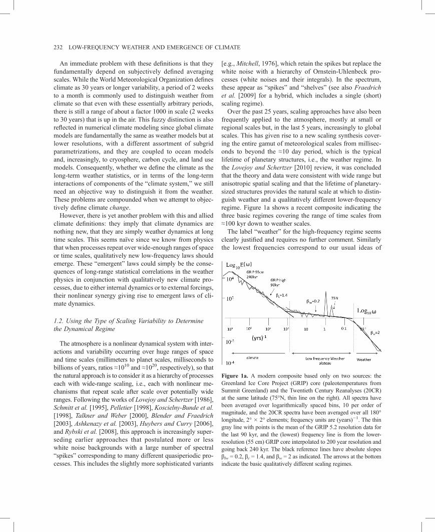
Figure 1a. A modern composite based only on two sources: theGreenland Ice Core Project (GRIP) core (paleotemperatures fromSummit Greenland) and the Twentieth Century Reanalyses (20CR)at the same latitude (75°N, thin line on the right). All spectra havebeen averaged over logarithmically spaced bins, 10 per order ofmagnitude, and the 20CR spectra have been averaged over all 180°longitude, 2° � 2° elements; frequency units are (years)�1. The thingray line with points is the mean of the GRIP 5.2 resolution data forthe last 90 kyr, and the (lowest) frequency line is from the lower-resolution (55 cm) GRIP core interpolated to 200 year resolution andgoing back 240 kyr. The black reference lines have absolute slopesβlw = 0.2, βc = 1.4, and βw = 2 as indicated. The arrows at the bottomindicate the basic qualitatively different scaling regimes.
232 LOW-FREQUENCY WEATHER AND EMERGENCE OF CLIMATE
An immediate problem with these definitions is that theyfundamentally depend on subjectively defined averagingscales. While the World Meteorological Organization definesclimate as 30 years or longer variability, a period of 2 weeksto a month is commonly used to distinguish weather fromclimate so that even with these essentially arbitrary periods,there is still a range of about a factor 1000 in scale (2 weeksto 30 years) that is up in the air. This fuzzy distinction is alsoreflected in numerical climate modeling since global climatemodels are fundamentally the same as weather models but atlower resolutions, with a different assortment of subgridparametrizations, and they are coupled to ocean modelsand, increasingly, to cryosphere, carbon cycle, and land usemodels. Consequently, whether we define the climate as thelong-term weather statistics, or in terms of the long-terminteractions of components of the “climate system,” we stillneed an objective way to distinguish it from the weather.These problems are compounded when we attempt to objec-tively define climate change.However, there is yet another problem with this and allied
climate definitions: they imply that climate dynamics arenothing new, that they are simply weather dynamics at longtime scales. This seems naïve since we know from physicsthat when processes repeat over wide-enough ranges of spaceor time scales, qualitatively new low-frequency laws shouldemerge. These “emergent” laws could simply be the conse-quences of long-range statistical correlations in the weatherphysics in conjunction with qualitatively new climate pro-cesses, due to either internal dynamics or to external forcings,their nonlinear synergy giving rise to emergent laws of cli-mate dynamics.
1.2. Using the Type of Scaling Variability to Determinethe Dynamical Regime
The atmosphere is a nonlinear dynamical system with inter-actions and variability occurring over huge ranges of spaceand time scales (millimeters to planet scales, milliseconds tobillions of years, ratios ≈1010 and ≈1020, respectively), so thatthe natural approach is to consider it as a hierarchy of processeseach with wide-range scaling, i.e., each with nonlinear me-chanisms that repeat scale after scale over potentially wideranges. Following the works of Lovejoy and Schertzer [1986],Schmitt et al. [1995], Pelletier [1998], Koscielny-Bunde et al.[1998], Talkner and Weber [2000], Blender and Fraedrich[2003], Ashkenazy et al. [2003], Huybers and Curry [2006],and Rybski et al. [2008], this approach is increasingly super-seding earlier approaches that postulated more or lesswhite noise backgrounds with a large number of spectral“spikes” corresponding to many different quasiperiodic pro-cesses. This includes the slightly more sophisticated variants
[e.g., Mitchell, 1976], which retain the spikes but replace thewhite noise with a hierarchy of Ornstein-Uhlenbeck pro-cesses (white noises and their integrals). In the spectrum,these appear as “spikes” and “shelves” (see also Fraedrichet al. [2009] for a hybrid, which includes a single (short)scaling regime).Over the past 25 years, scaling approaches have also been
frequently applied to the atmosphere, mostly at small orregional scales but, in the last 5 years, increasingly to globalscales. This has given rise to a new scaling synthesis cover-ing the entire gamut of meteorological scales from millisec-onds to beyond the ≈10 day period, which is the typicallifetime of planetary structures, i.e., the weather regime. Inthe Lovejoy and Schertzer [2010] review, it was concludedthat the theory and data were consistent with wide range butanisotropic spatial scaling and that the lifetime of planetary-sized structures provides the natural scale at which to distin-guish weather and a qualitatively different lower-frequencyregime. Figure 1a shows a recent composite indicating thethree basic regimes covering the range of time scales from≈100 kyr down to weather scales.The label “weather” for the high-frequency regime seems
clearly justified and requires no further comment. Similarlythe lowest frequencies correspond to our usual ideas of
LOVEJOY AND SCHERTZER 233
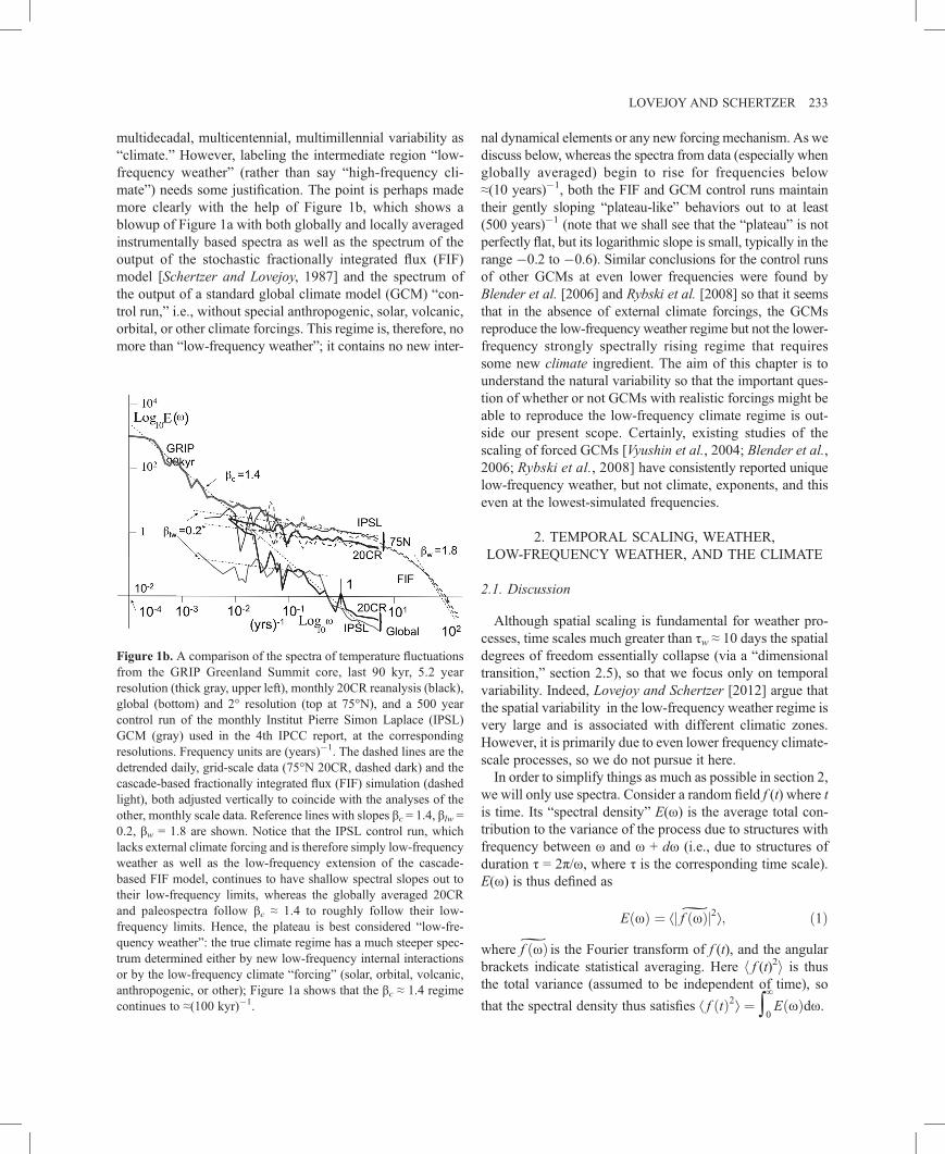
multidecadal, multicentennial, multimillennial variability as“climate.” However, labeling the intermediate region “low-frequency weather” (rather than say “high-frequency cli-mate”) needs some justification. The point is perhaps mademore clearly with the help of Figure 1b, which shows ablowup of Figure 1a with both globally and locally averagedinstrumentally based spectra as well as the spectrum of theoutput of the stochastic fractionally integrated flux (FIF)model [Schertzer and Lovejoy, 1987] and the spectrum ofthe output of a standard global climate model (GCM) “con-trol run,” i.e., without special anthropogenic, solar, volcanic,orbital, or other climate forcings. This regime is, therefore, nomore than “low-frequency weather”; it contains no new inter-
Figure 1b. A comparison of the spectra of temperature fluctuationsfrom the GRIP Greenland Summit core, last 90 kyr, 5.2 yearresolution (thick gray, upper left), monthly 20CR reanalysis (black),global (bottom) and 2° resolution (top at 75°N), and a 500 yearcontrol run of the monthly Institut Pierre Simon Laplace (IPSL)GCM (gray) used in the 4th IPCC report, at the correspondingresolutions. Frequency units are (years)�1. The dashed lines are thedetrended daily, grid-scale data (75°N 20CR, dashed dark) and thecascade-based fractionally integrated flux (FIF) simulation (dashedlight), both adjusted vertically to coincide with the analyses of theother, monthly scale data. Reference lines with slopes βc = 1.4, βlw =0.2, βw = 1.8 are shown. Notice that the IPSL control run, whichlacks external climate forcing and is therefore simply low-frequencyweather as well as the low-frequency extension of the cascade-based FIF model, continues to have shallow spectral slopes out totheir low-frequency limits, whereas the globally averaged 20CRand paleospectra follow βc ≈ 1.4 to roughly follow their low-frequency limits. Hence, the plateau is best considered “low-fre-quency weather”: the true climate regime has a much steeper spec-trum determined either by new low-frequency internal interactionsor by the low-frequency climate “forcing” (solar, orbital, volcanic,anthropogenic, or other); Figure 1a shows that the βc ≈ 1.4 regimecontinues to ≈(100 kyr)�1.
nal dynamical elements or any new forcing mechanism. As wediscuss below, whereas the spectra from data (especially whenglobally averaged) begin to rise for frequencies below≈(10 years)�1, both the FIF and GCM control runs maintaintheir gently sloping “plateau-like” behaviors out to at least(500 years)�1 (note that we shall see that the “plateau” is notperfectly flat, but its logarithmic slope is small, typically in therange �0.2 to �0.6). Similar conclusions for the control runsof other GCMs at even lower frequencies were found byBlender et al. [2006] and Rybski et al. [2008] so that it seemsthat in the absence of external climate forcings, the GCMsreproduce the low-frequency weather regime but not the lower-frequency strongly spectrally rising regime that requiressome new climate ingredient. The aim of this chapter is tounderstand the natural variability so that the important ques-tion of whether or not GCMs with realistic forcings might beable to reproduce the low-frequency climate regime is out-side our present scope. Certainly, existing studies of thescaling of forced GCMs [Vyushin et al., 2004; Blender et al.,2006; Rybski et al., 2008] have consistently reported uniquelow-frequency weather, but not climate, exponents, and thiseven at the lowest-simulated frequencies.
2. TEMPORAL SCALING, WEATHER,LOW-FREQUENCY WEATHER, AND THE CLIMATE
2.1. Discussion
Although spatial scaling is fundamental for weather pro-cesses, time scales much greater than τw ≈ 10 days the spatialdegrees of freedom essentially collapse (via a “dimensionaltransition,” section 2.5), so that we focus only on temporalvariability. Indeed, Lovejoy and Schertzer [2012] argue thatthe spatial variability in the low-frequency weather regime isvery large and is associated with different climatic zones.However, it is primarily due to even lower frequency climate-scale processes, so we do not pursue it here.In order to simplify things as much as possible in section 2,
we will only use spectra. Consider a random field f (t) where tis time. Its “spectral density” E(ω) is the average total con-tribution to the variance of the process due to structures withfrequency between ω and ω + dω (i.e., due to structures ofduration τ = 2π/ω, where τ is the corresponding time scale).E(ω) is thus defined as
EðωÞ ¼ ⟨j f ðωÞ̃j2⟩; ð1Þwhere f ðωÞ̃ is the Fourier transform of f (t), and the angularbrackets indicate statistical averaging. Here h f (t)2i is thusthe total variance (assumed to be independent of time), so
that the spectral density thus satisfies ⟨ f ðtÞ2⟩ ¼ ∫∞
0EðωÞdω.
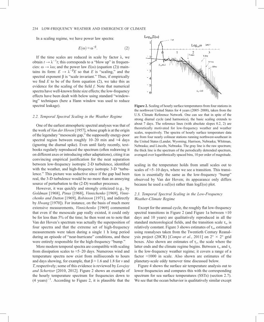
Figure 2. Scaling of hourly surface temperatures from four stations inthe northwest United States for 4 years (2005–2008), taken from theU.S. Climate Reference Network. One can see that in spite of thestrong diurnal cycle (and harmonics), the basic scaling extends toabout 7 days. The reference lines (with absolute slopes 0.2, 2) aretheoretically motivated for low-frequency weather and weatherscales, respectively. The spectra of hourly surface temperature dataare from four nearly colinear stations running northwest-southeast inthe United States (Lander, Wyoming; Harrison, Nebraska; Whitman,Nebraska; and Lincoln, Nebraska. The gray line is the raw spectrum;the thick line is the spectrum of the periodically detrended spectrum,averaged over logarithmically spaced bins, 10 per order of magnitude.
234 LOW-FREQUENCY WEATHER AND EMERGENCE OF CLIMATE
In a scaling regime, we have power law spectra:
EðωÞ ≈ ω−β: ð2Þ
If the time scales are reduced in scale by factor λ, weobtain t → λ�1t; this corresponds to a “blow up” in frequen-cies: ω → λω; and the power law E(ω) (equation (2)) main-tains its form: E → λ�βE so that E is “scaling,” and thespectral exponent β is “scale invariant.” Thus, if empiricallywe find E to be of the form equation (2), we take this asevidence for the scaling of the field f. Note that numericalspectra have well-known finite size effects; the low-frequencyeffects have been dealt with below using standard “window-ing” techniques (here a Hann window was used to reducespectral leakage).
2.2. Temporal Spectral Scaling in the Weather Regime
One of the earliest atmospheric spectral analyses was that ofthe work of Van der Hoven [1957], whose graph is at the originof the legendary “mesoscale gap,” the supposedly energy-poorspectral region between roughly 10–20 min and ≈4 days(ignoring the diurnal spike). Even until fairly recently, text-books regularly reproduced the spectrum (often redrawing iton different axes or introducing other adaptations), citing it asconvincing empirical justification for the neat separationbetween low-frequency isotropic 2-D turbulence, identifiedwith the weather, and high-frequency isotropic 3-D “turbu-lence.” This picture was seductive since if the gap had beenreal, the 3-D turbulence would be no more than an annoyingsource of perturbation to the (2-D) weather processes.However, it was quickly and strongly criticized (e.g., by
Goldman [1968], Pinus [1968], Vinnichenko [1969], Vinni-chenko and Dutton [1969], Robinson [1971], and indirectlyby Hwang [1970]). For instance, on the basis of much moreextensive measurements, Vinnichenko [1969] commentedthat even if the mesoscale gap really existed, it could onlybe for less than 5% of the time; he then went on to note thatVan der Hoven’s spectrum was actually the superposition offour spectra and that the extreme set of high-frequencymeasurements were taken during a single 1 h long periodduring an episode of “near-hurricane” conditions, and thesewere entirely responsible for the high-frequency “bump.”More modern temporal spectra are compatible with scaling
from dissipation scales to ≈5–20 days. Numerous wind andtemperature spectra now exist from milliseconds to hoursand days showing, for example, that β ≈ 1.6 and 1.8 for v andT, respectively; some of this evidence is reviewed by Lovejoyand Schertzer [2010, 2012]. Figure 2 shows an example ofthe hourly temperature spectrum for frequencies down to(4 years)�1. According to Figure 2, it is plausible that the
scaling in the temperature holds from small scales out toscales of ≈5–10 days, where we see a transition. This transi-tion is essentially the same as the low-frequency “bump”observed by Van der Hoven; its appearance only differsbecause he used a ωE(ω) rather than logE(ω) plot.
2.3. Temporal Spectral Scaling in the Low-FrequencyWeather-Climate Regime
Except for the annual cycle, the roughly flat low-frequencyspectral transitions in Figure 2 (and Figure 1a between ≈10days and 10 years) are qualitatively reproduced in all thestandard meteorological fields, and the transition scale τw isrelatively constant. Figure 3 shows estimates of τw, estimatedusing reanalyses taken from the Twentieth Century Reanal-ysis project (20CR) [Compo et al., 2011] on 2° � 2° gridboxes. Also shown are estimates of τc, the scale where thelatter ends and the climate regime begins. Between τw and τcis the low-frequency weather regime; it covers a range of afactor ≈1000 in scale. Also shown are estimates of theplanetary-scale eddy turnover time discussed below.Figure 4 shows the surface air temperature analysis out to
lower frequencies and compares this with the correspondingspectrum for sea surface temperatures (SSTs) (section 2.7).We see that the ocean behavior is qualitatively similar except
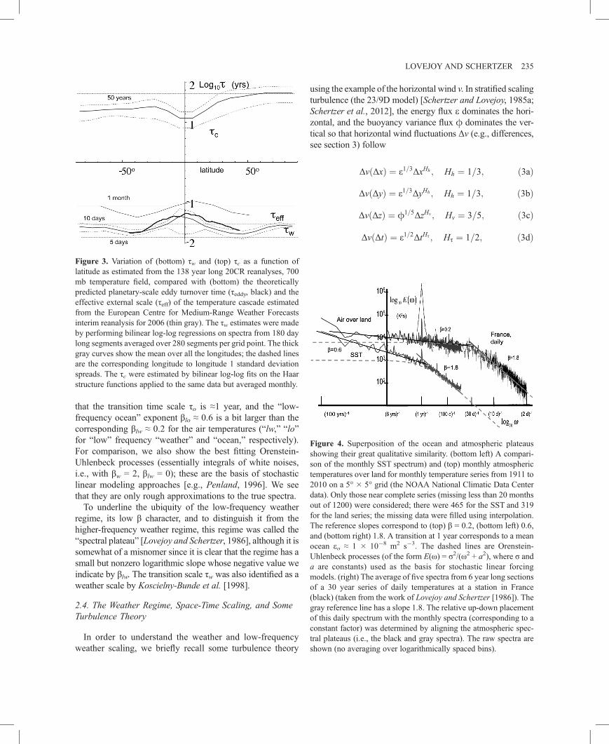
Figure 3. Variation of (bottom) τw and (top) τc as a function oflatitude as estimated from the 138 year long 20CR reanalyses, 700mb temperature field, compared with (bottom) the theoreticallypredicted planetary-scale eddy turnover time (τeddy, black) and theeffective external scale (τeff) of the temperature cascade estimatedfrom the European Centre for Medium-Range Weather Forecastsinterim reanalysis for 2006 (thin gray). The τw estimates were madeby performing bilinear log-log regressions on spectra from 180 daylong segments averaged over 280 segments per grid point. The thickgray curves show the mean over all the longitudes; the dashed linesare the corresponding longitude to longitude 1 standard deviationspreads. The τc were estimated by bilinear log-log fits on the Haarstructure functions applied to the same data but averaged monthly.
Figure 4. Superposition of the ocean and atmospheric plateausshowing their great qualitative similarity. (bottom left) A compari-son of the monthly SST spectrum) and (top) monthly atmospherictemperatures over land for monthly temperature series from 1911 to2010 on a 5° � 5° grid (the NOAA National Climatic Data Centerdata). Only those near complete series (missing less than 20 monthsout of 1200) were considered; there were 465 for the SST and 319for the land series; the missing data were filled using interpolation.The reference slopes correspond to (top) β = 0.2, (bottom left) 0.6,and (bottom right) 1.8. A transition at 1 year corresponds to a meanocean eo ≈ 1 � 10�8 m2 s�3. The dashed lines are Orenstein-Uhlenbeck processes (of the form E(ω) = σ2/(ω2 + a2), where σ anda are constants) used as the basis for stochastic linear forcingmodels. (right) The average of five spectra from 6 year long sectionsof a 30 year series of daily temperatures at a station in France(black) (taken from the work of Lovejoy and Schertzer [1986]). Thegray reference line has a slope 1.8. The relative up-down placementof this daily spectrum with the monthly spectra (corresponding to aconstant factor) was determined by aligning the atmospheric spec-tral plateaus (i.e., the black and gray spectra). The raw spectra areshown (no averaging over logarithmically spaced bins).
LOVEJOY AND SCHERTZER 235
that the transition time scale τo is ≈1 year, and the “low-frequency ocean” exponent βlo ≈ 0.6 is a bit larger than thecorresponding βlw ≈ 0.2 for the air temperatures (“lw,” “lo”for “low” frequency “weather” and “ocean,” respectively).For comparison, we also show the best fitting Orenstein-Uhlenbeck processes (essentially integrals of white noises,i.e., with βw = 2, βlw = 0); these are the basis of stochasticlinear modeling approaches [e.g., Penland, 1996]. We seethat they are only rough approximations to the true spectra.To underline the ubiquity of the low-frequency weather
regime, its low β character, and to distinguish it from thehigher-frequency weather regime, this regime was called the“spectral plateau” [Lovejoy and Schertzer, 1986], although it issomewhat of a misnomer since it is clear that the regime has asmall but nonzero logarithmic slope whose negative value weindicate by βlw. The transition scale τw was also identified as aweather scale by Koscielny-Bunde et al. [1998].
2.4. The Weather Regime, Space-Time Scaling, and SomeTurbulence Theory
In order to understand the weather and low-frequencyweather scaling, we briefly recall some turbulence theory
using the example of the horizontal wind v. In stratified scalingturbulence (the 23/9D model) [Schertzer and Lovejoy, 1985a;Schertzer et al., 2012], the energy flux e dominates the hori-zontal, and the buoyancy variance flux φ dominates the ver-tical so that horizontal wind fluctuations Δv (e.g., differences,see section 3) follow
ΔvðΔxÞ ¼ ε1=3ΔxHh ; Hh ¼ 1=3; ð3aÞ
ΔvðΔyÞ ¼ ε1=3ΔyHh ; Hh ¼ 1=3; ð3bÞ
ΔvðΔzÞ ¼ φ1=5ΔzHv ; Hv ¼ 3=5; ð3cÞ
ΔvðΔtÞ ¼ ε1=2ΔtHτ ; Hτ ¼ 1=2; ð3dÞ
236 LOW-FREQUENCY WEATHER AND EMERGENCE OF CLIMATE
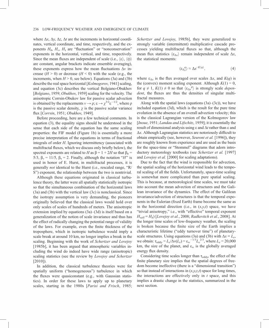
where Δx, Δy, Δz, Δt are the increments in horizontal coordi-nates, vertical coordinate, and time, respectively, and the ex-ponents Hh, Hv, Hτ are “fluctuation” or “nonconservation”exponents in the horizontal, vertical, and time, respectively.Since the mean fluxes are independent of scale (i.e., hei, hφiare constant, angular brackets indicate ensemble averaging),these exponents express how the mean fluctuations Δv in-crease (H > 0) or decrease (H < 0) with the scale (e.g., theincrements, when H > 0, see below). Equations (3a) and (3b)describe the real space horizontal [Kolmogorov, 1941] scaling,and equation (3c) describes the vertical Bolgiano-Obukhov[Bolgiano, 1959;Obukhov, 1959] scaling for the velocity. Theanisotropic Corrsin-Obukov law for passive scalar advectionis obtained by the replacements v→ ρ; e→ v3/2e�1/2, where ρis the passive scalar density, v is the passive scalar varianceflux [Corrsin, 1951; Obukhov, 1949].Before proceeding, here are a few technical comments. In
equation (3), the equality signs should be understood in thesense that each side of the equation has the same scalingproperties: the FIF model (Figure 1b) is essentially a moreprecise interpretation of the equations in terms of fractionalintegrals of order H. Ignoring intermittency (associated withmultifractal fluxes, which we discuss only briefly below), thespectral exponents are related to H as β = 1 + 2H so that βh =5/3, βv = 11/5, βτ = 2. Finally, although the notation “H” isused in honor of E. Hurst, in multifractal processes, it isgenerally not identical to the Hurst (i.e., rescaled range, “R/S”) exponent, the relationship between the two is nontrivial.Although these equations originated in classical turbu-
lence theory, the latter were all spatially statistically isotropicso that the simultaneous combination of the horizontal laws(3a) and (3b) with the vertical law (3c) is nonclassical. Sincethe isotropy assumption is very demanding, the pioneersoriginally believed that the classical laws would hold overonly scales of scales of hundreds of meters. The anisotropicextension implied by equations (3a)–(3d) is itself based on ageneralization of the notion of scale invariance and thus hasthe effect of radically changing the potential range of validityof the laws. For example, even the finite thickness of thetroposphere, which in isotropic turbulence would imply ascale break at around 10 km, no longer implies a break in thescaling. Beginning with the work of Schertzer and Lovejoy[1985b], it has been argued that atmospheric variables in-cluding the wind do indeed have wide range (anisotropic)scaling statistics (see the review by Lovejoy and Schertzer[2010]).In addition, the classical turbulence theories were for
spatially uniform (“homogeneous”) turbulence in whichthe fluxes were quasiconstant (e.g., with Gaussian statis-tics). In order for these laws to apply up to planetaryscales, starting in the 1980s [Parisi and Frisch, 1985;
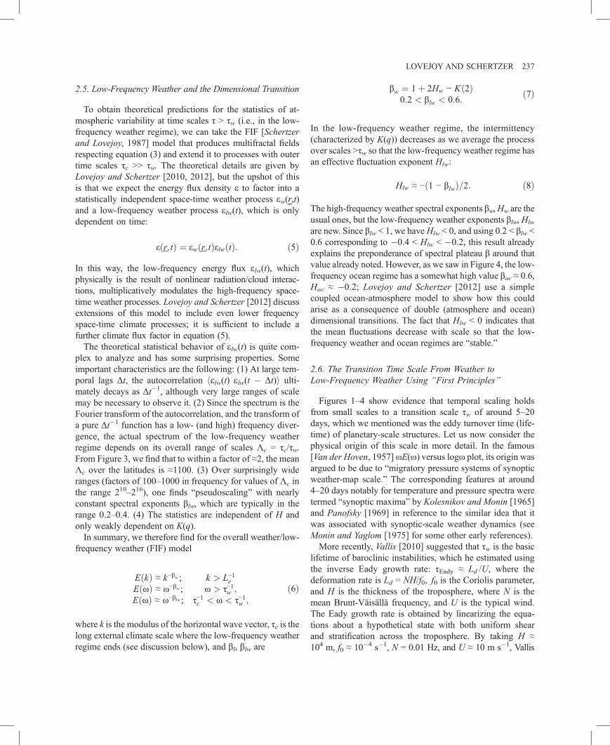
Schertzer and Lovejoy, 1985b], they were generalized tostrongly variable (intermittent) multiplicative cascade pro-cesses yielding multifractal fluxes so that, although themean flux statistics heΔxi remain independent of scale Δx,the statistical moments:
⟨εΔqx ⟩ ≈ Δx−KðqÞ; ð4Þ
where eΔx is the flux averaged over scales Δx, and K(q) isthe (convex) moment scaling exponent. Although K(1) = 0,for q ≠ 1, K(1) ≠ 0 so that heΔxqi is strongly scale depen-dent, the fluxes are thus the densities of singular multi-fractal measures.Along with the spatial laws (equations (3a)–(3c)), we have
included equation (3d), which is the result for the pure timeevolution in the absence of an overall advection velocity; thisis the classical Lagrangian version of the Kolmogorov law[Inoue, 1951; Landau and Lifschitz, 1959]; it is essentially theresult of dimensional analysis using e and Δt rather than e andΔx. Although Lagrangian statistics are notoriously difficult toobtain empirically (see, however, Seuront et al. [1996]), theyare roughly known from experience and are used as the basisfor the space-time or “Stommel” diagrams that adorn intro-ductory meteorology textbooks (see Schertzer et al. [1997]and Lovejoy et al. [2000] for scaling adaptations).Due to the fact that the wind is responsible for advection,
the spatial scaling of the horizontal wind leads to the tempo-ral scaling of all the fields. Unfortunately, space-time scalingis somewhat more complicated than pure spatial scaling.This is because, at meteorological time scales, we must takeinto account the mean advection of structures and the Gali-lean invariance of the dynamics. The effect of the Galileaninvariance/advection of structures is that the temporal expo-nents in the Eulerian (fixed Earth) frame become the same asin the horizontal direction (i.e., in (x,y,t) space, we have“trivial anisotropy,” i.e., with “effective” temporal exponentHτeff = Hh) [Lovejoy et al., 2008; Radkevitch et al., 2008]. Atthe longer time scales of low-frequency weather, the scalingis broken because the finite size of the Earth implies acharacteristic lifetime (“eddy turnover time”) of planetary-scale structures. Using equations (3a) and (3b) with Δx = Le,we obtain: τeddy = Le/Δv(Le) = ew�1/3Le
2/3, where Le = 20,000km, the size of the planet, and ew is the globally averagedenergy flux density.Considering time scales longer than τeddy, the effect of the
finite planetary size implies that the spatial degrees of free-dom become ineffective (there is a “dimensional transition”)so that instead of interactions in (x,y,z,t) space for long times,the interactions are effectively only in t space, and thisimplies a drastic change in the statistics, summarized in thenext section.
LOVEJOY AND SCHERTZER 237
2.5. Low-Frequency Weather and the Dimensional Transition
To obtain theoretical predictions for the statistics of at-mospheric variability at time scales τ > τw (i.e., in the low-frequency weather regime), we can take the FIF [Schertzerand Lovejoy, 1987] model that produces multifractal fieldsrespecting equation (3) and extend it to processes with outertime scales τc >> τw. The theoretical details are given byLovejoy and Schertzer [2010, 2012], but the upshot of thisis that we expect the energy flux density e to factor into astatistically independent space-time weather process ew(r,t)and a low-frequency weather process elw(t), which is onlydependent on time:
εð¯r;tÞ ¼ εwð
¯r;tÞεlwðtÞ: ð5Þ
In this way, the low-frequency energy flux elw(t), whichphysically is the result of nonlinear radiation/cloud interac-tions, multiplicatively modulates the high-frequency space-time weather processes. Lovejoy and Schertzer [2012] discussextensions of this model to include even lower frequencyspace-time climate processes; it is sufficient to include afurther climate flux factor in equation (5).The theoretical statistical behavior of elw(t) is quite com-
plex to analyze and has some surprising properties. Someimportant characteristics are the following: (1) At large tem-poral lags Δt, the autocorrelation helw(t) elw(t � Δt)i ulti-mately decays as Δt�1, although very large ranges of scalemay be necessary to observe it. (2) Since the spectrum is theFourier transform of the autocorrelation, and the transform ofa pure Δt�1 function has a low- (and high) frequency diver-gence, the actual spectrum of the low-frequency weatherregime depends on its overall range of scales Λc = τc/τw.From Figure 3, we find that to within a factor of ≈2, the meanΛc over the latitudes is ≈1100. (3) Over surprisingly wideranges (factors of 100–1000 in frequency for values of Λc inthe range 210–216), one finds “pseudoscaling” with nearlyconstant spectral exponents βlw, which are typically in therange 0.2–0.4. (4) The statistics are independent of H andonly weakly dependent on K(q).In summary, we therefore find for the overall weather/low-
frequency weather (FIF) model
EðkÞ ≈ k−βw ; k > L−1eEðωÞ ≈ ω−βw ; ω > τ−1w ;EðωÞ ≈ ω−βlw ; τ−1c < ω < τ−1w ;
ð6Þ
where k is the modulus of the horizontal wave vector, τc is thelong external climate scale where the low-frequency weatherregime ends (see discussion below), and βl, βlw are
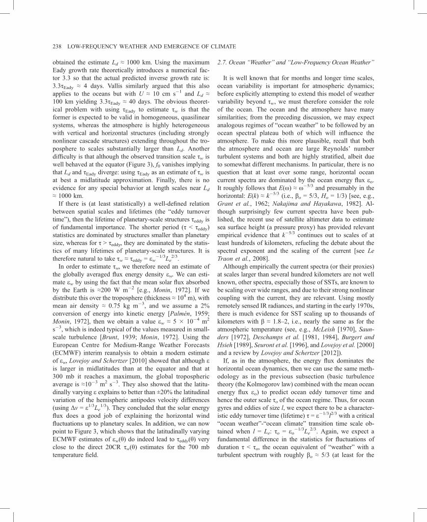
βw ¼ 1þ 2Hw − Kð2Þ0:2 < βlw < 0:6:
ð7Þ
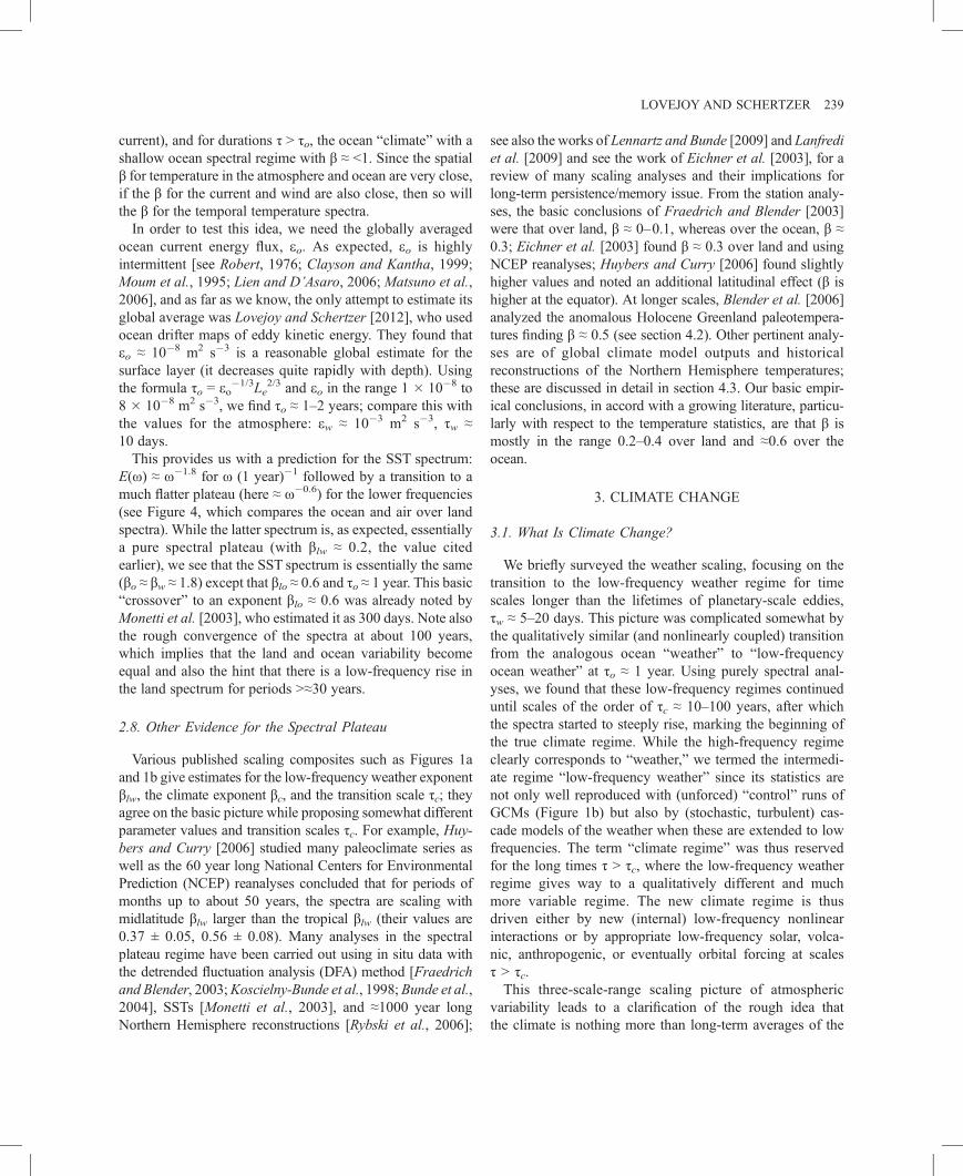
In the low-frequency weather regime, the intermittency(characterized by K(q)) decreases as we average the processover scales >τw so that the low-frequency weather regime hasan effective fluctuation exponent Hlw:
Hlw ≈ −ð1 − βlwÞ=2: ð8Þ
The high-frequency weather spectral exponents βw,Hw are theusual ones, but the low-frequency weather exponents βlw, Hlw
are new. Since βlw < 1, we haveHlw < 0, and using 0.2 < βlw <0.6 corresponding to �0.4 < Hlw < �0.2, this result alreadyexplains the preponderance of spectral plateau β around thatvalue already noted. However, as we saw in Figure 4, the low-frequency ocean regime has a somewhat high value βoc ≈ 0.6,Hoc ≈ �0.2; Lovejoy and Schertzer [2012] use a simplecoupled ocean-atmosphere model to show how this couldarise as a consequence of double (atmosphere and ocean)dimensional transitions. The fact that Hlw < 0 indicates thatthe mean fluctuations decrease with scale so that the low-frequency weather and ocean regimes are “stable.”
2.6. The Transition Time Scale From Weather toLow-Frequency Weather Using “First Principles”
Figures 1–4 show evidence that temporal scaling holdsfrom small scales to a transition scale τw of around 5–20days, which we mentioned was the eddy turnover time (life-time) of planetary-scale structures. Let us now consider thephysical origin of this scale in more detail. In the famous[Van der Hoven, 1957] ωE(ω) versus logω plot, its origin wasargued to be due to “migratory pressure systems of synopticweather-map scale.” The corresponding features at around4–20 days notably for temperature and pressure spectra weretermed “synoptic maxima” by Kolesnikov and Monin [1965]and Panofsky [1969] in reference to the similar idea that itwas associated with synoptic-scale weather dynamics (seeMonin and Yaglom [1975] for some other early references).More recently, Vallis [2010] suggested that τw is the basic
lifetime of baroclinic instabilities, which he estimated usingthe inverse Eady growth rate: τEady ≈ Ld /U, where thedeformation rate is Ld = NH/f0, f0 is the Coriolis parameter,and H is the thickness of the troposphere, where N is themean Brunt-Väisällä frequency, and U is the typical wind.The Eady growth rate is obtained by linearizing the equa-tions about a hypothetical state with both uniform shearand stratification across the troposphere. By taking H ≈104 m, f0 ≈ 10�4 s�1, N = 0.01 Hz, and U ≈ 10 m s�1, Vallis
238 LOW-FREQUENCY WEATHER AND EMERGENCE OF CLIMATE
obtained the estimate Ld ≈ 1000 km. Using the maximumEady growth rate theoretically introduces a numerical fac-tor 3.3 so that the actual predicted inverse growth rate is:3.3τEady ≈ 4 days. Vallis similarly argued that this alsoapplies to the oceans but with U ≈ 10 cm s�1 and Ld ≈100 km yielding 3.3τEady ≈ 40 days. The obvious theoret-ical problem with using τEady to estimate τw is that theformer is expected to be valid in homogeneous, quasilinearsystems, whereas the atmosphere is highly heterogeneouswith vertical and horizontal structures (including stronglynonlinear cascade structures) extending throughout the tro-posphere to scales substantially larger than Ld. Anotherdifficulty is that although the observed transition scale τw iswell behaved at the equator (Figure 3), f0 vanishes implyingthat Ld and τEady diverge: using τEady as an estimate of τw isat best a midlatitude approximation. Finally, there is noevidence for any special behavior at length scales near Ld≈ 1000 km.If there is (at least statistically) a well-defined relation
between spatial scales and lifetimes (the “eddy turnovertime”), then the lifetime of planetary-scale structures τeddy isof fundamental importance. The shorter period (τ < τeddy)statistics are dominated by structures smaller than planetarysize, whereas for τ > τeddy, they are dominated by the statis-tics of many lifetimes of planetary-scale structures. It istherefore natural to take τw ≈ τeddy = ew�1/3Le
2/3.In order to estimate τw, we therefore need an estimate of
the globally averaged flux energy density ew. We can esti-mate ew by using the fact that the mean solar flux absorbedby the Earth is ≈200 W m�2 [e.g., Monin, 1972]. If wedistribute this over the troposphere (thickness ≈ 104 m), withmean air density ≈ 0.75 kg m�3, and we assume a 2%conversion of energy into kinetic energy [Palmén, 1959;Monin, 1972], then we obtain a value ew ≈ 5 � 10�4 m2
s�3, which is indeed typical of the values measured in small-scale turbulence [Brunt, 1939; Monin, 1972]. Using theEuropean Centre for Medium-Range Weather Forecasts(ECMWF) interim reanalysis to obtain a modern estimateof ew, Lovejoy and Schertzer [2010] showed that although eis larger in midlatitudes than at the equator and that at300 mb it reaches a maximum, the global troposphericaverage is ≈10�3 m2 s�3. They also showed that the latitu-dinally varying e explains to better than ±20% the latitudinalvariation of the hemispheric antipodes velocity differences(using Δv = e1/3Le1/3). They concluded that the solar energyflux does a good job of explaining the horizontal windfluctuations up to planetary scales. In addition, we can nowpoint to Figure 3, which shows that the latitudinally varyingECMWF estimates of ew(θ) do indeed lead to τeddy(θ) veryclose to the direct 20CR τw(θ) estimates for the 700 mbtemperature field.
2.7. Ocean “Weather” and “Low-Frequency Ocean Weather”
It is well known that for months and longer time scales,ocean variability is important for atmospheric dynamics;before explicitly attempting to extend this model of weathervariability beyond τw, we must therefore consider the roleof the ocean. The ocean and the atmosphere have manysimilarities; from the preceding discussion, we may expectanalogous regimes of “ocean weather” to be followed by anocean spectral plateau both of which will influence theatmosphere. To make this more plausible, recall that boththe atmosphere and ocean are large Reynolds’ numberturbulent systems and both are highly stratified, albeit dueto somewhat different mechanisms. In particular, there is noquestion that at least over some range, horizontal oceancurrent spectra are dominated by the ocean energy flux eo.It roughly follows that E(ω) ≈ ω�5/3 and presumably in thehorizontal: E(k) ≈ k�5/3 (i.e., βo = 5/3, Ho = 1/3) [see, e.g.,Grant et al., 1962; Nakajima and Hayakawa, 1982]. Al-though surprisingly few current spectra have been pub-lished, the recent use of satellite altimeter data to estimatesea surface height (a pressure proxy) has provided relevantempirical evidence that k�5/3 continues out to scales of atleast hundreds of kilometers, refueling the debate about thespectral exponent and the scaling of the current [see LeTraon et al., 2008].Although empirically the current spectra (or their proxies)
at scales larger than several hundred kilometers are not wellknown, other spectra, especially those of SSTs, are known tobe scaling over wide ranges, and due to their strong nonlinearcoupling with the current, they are relevant. Using mostlyremotely sensed IR radiances, and starting in the early 1970s,there is much evidence for SST scaling up to thousands ofkilometers with β ≈ 1.8–2, i.e., nearly the same as for theatmospheric temperature (see, e.g., McLeish [1970], Saun-ders [1972], Deschamps et al. [1981, 1984], Burgert andHsieh [1989], Seuront et al. [1996], and Lovejoy et al. [2000]and a review by Lovejoy and Schertzer [2012]).If, as in the atmosphere, the energy flux dominates the
horizontal ocean dynamics, then we can use the same meth-odology as in the previous subsection (basic turbulencetheory (the Kolmogorov law) combined with the mean oceanenergy flux eo) to predict ocean eddy turnover time andhence the outer scale τo of the ocean regime. Thus, for oceangyres and eddies of size l, we expect there to be a character-istic eddy turnover time (lifetime) τ = e�1/3l2/3 with a critical“ocean weather”-“ocean climate” transition time scale ob-tained when l = Le: τo = eo�1/3Le
2/3. Again, we expect afundamental difference in the statistics for fluctuations ofduration τ < τo, the ocean equivalent of “weather” with aturbulent spectrum with roughly βo ≈ 5/3 (at least for the
LOVEJOY AND SCHERTZER 239
current), and for durations τ > τo, the ocean “climate” with ashallow ocean spectral regime with β ≈ <1. Since the spatialβ for temperature in the atmosphere and ocean are very close,if the β for the current and wind are also close, then so willthe β for the temporal temperature spectra.In order to test this idea, we need the globally averaged
ocean current energy flux, eo. As expected, eo is highlyintermittent [see Robert, 1976; Clayson and Kantha, 1999;Moum et al., 1995; Lien and D’Asaro, 2006; Matsuno et al.,2006], and as far as we know, the only attempt to estimate itsglobal average was Lovejoy and Schertzer [2012], who usedocean drifter maps of eddy kinetic energy. They found thateo ≈ 10�8 m2 s�3 is a reasonable global estimate for thesurface layer (it decreases quite rapidly with depth). Usingthe formula τo = eo�1/3Le
2/3 and eo in the range 1 � 10�8 to8 � 10�8 m2 s�3, we find τo ≈ 1–2 years; compare this withthe values for the atmosphere: ew ≈ 10�3 m2 s�3, τw ≈10 days.This provides us with a prediction for the SST spectrum:
E(ω) ≈ ω�1.8 for ω (1 year)�1 followed by a transition to amuch flatter plateau (here ≈ ω�0.6) for the lower frequencies(see Figure 4, which compares the ocean and air over landspectra). While the latter spectrum is, as expected, essentiallya pure spectral plateau (with βlw ≈ 0.2, the value citedearlier), we see that the SST spectrum is essentially the same(βo ≈ βw ≈ 1.8) except that βlo ≈ 0.6 and τo ≈ 1 year. This basic“crossover” to an exponent βlo ≈ 0.6 was already noted byMonetti et al. [2003], who estimated it as 300 days. Note alsothe rough convergence of the spectra at about 100 years,which implies that the land and ocean variability becomeequal and also the hint that there is a low-frequency rise inthe land spectrum for periods >≈30 years.
2.8. Other Evidence for the Spectral Plateau
Various published scaling composites such as Figures 1aand 1b give estimates for the low-frequency weather exponentβlw, the climate exponent βc, and the transition scale τc; theyagree on the basic picture while proposing somewhat differentparameter values and transition scales τc. For example, Huy-bers and Curry [2006] studied many paleoclimate series aswell as the 60 year long National Centers for EnvironmentalPrediction (NCEP) reanalyses concluded that for periods ofmonths up to about 50 years, the spectra are scaling withmidlatitude βlw larger than the tropical βlw (their values are0.37 ± 0.05, 0.56 ± 0.08). Many analyses in the spectralplateau regime have been carried out using in situ data withthe detrended fluctuation analysis (DFA) method [Fraedrichand Blender, 2003;Koscielny-Bunde et al., 1998; Bunde et al.,2004], SSTs [Monetti et al., 2003], and ≈1000 year longNorthern Hemisphere reconstructions [Rybski et al., 2006];
see also the works of Lennartz and Bunde [2009] and Lanfrediet al. [2009] and see the work of Eichner et al. [2003], for areview of many scaling analyses and their implications forlong-term persistence/memory issue. From the station analy-ses, the basic conclusions of Fraedrich and Blender [2003]were that over land, β ≈ 0–0.1, whereas over the ocean, β ≈0.3; Eichner et al. [2003] found β ≈ 0.3 over land and usingNCEP reanalyses; Huybers and Curry [2006] found slightlyhigher values and noted an additional latitudinal effect (β ishigher at the equator). At longer scales, Blender et al. [2006]analyzed the anomalous Holocene Greenland paleotempera-tures finding β ≈ 0.5 (see section 4.2). Other pertinent analy-ses are of global climate model outputs and historicalreconstructions of the Northern Hemisphere temperatures;these are discussed in detail in section 4.3. Our basic empir-ical conclusions, in accord with a growing literature, particu-larly with respect to the temperature statistics, are that β ismostly in the range 0.2–0.4 over land and ≈0.6 over theocean.
3. CLIMATE CHANGE
3.1. What Is Climate Change?
We briefly surveyed the weather scaling, focusing on thetransition to the low-frequency weather regime for timescales longer than the lifetimes of planetary-scale eddies,τw ≈ 5–20 days. This picture was complicated somewhat bythe qualitatively similar (and nonlinearly coupled) transitionfrom the analogous ocean “weather” to “low-frequencyocean weather” at τo ≈ 1 year. Using purely spectral anal-yses, we found that these low-frequency regimes continueduntil scales of the order of τc ≈ 10–100 years, after whichthe spectra started to steeply rise, marking the beginning ofthe true climate regime. While the high-frequency regimeclearly corresponds to “weather,” we termed the intermedi-ate regime “low-frequency weather” since its statistics arenot only well reproduced with (unforced) “control” runs ofGCMs (Figure 1b) but also by (stochastic, turbulent) cas-cade models of the weather when these are extended to lowfrequencies. The term “climate regime” was thus reservedfor the long times τ > τc, where the low-frequency weatherregime gives way to a qualitatively different and muchmore variable regime. The new climate regime is thusdriven either by new (internal) low-frequency nonlinearinteractions or by appropriate low-frequency solar, volca-nic, anthropogenic, or eventually orbital forcing at scalesτ > τc.This three-scale-range scaling picture of atmospheric
variability leads to a clarification of the rough idea thatthe climate is nothing more than long-term averages of the
240 LOW-FREQUENCY WEATHER AND EMERGENCE OF CLIMATE
weather. It allows us to precisely define a climate state asthe average of the weather over the entire low-frequencyweather regime up to τc (i.e., up to decadal or centennialscales). This paves the way for a straightforward definitionof climate change as the long-term changes in this climatestate, i.e., of the statistics of these climate states at scalesτ > τc.
3.2. What Is τc?
In Figures 1a and 1b, we gave some evidence that τcwas inthe range (10 years)�1 to (100 years)�1; that is, it was nearthe extreme low-frequency limit of instrumental data. Wenow attempt to determine it more accurately. Up until now,we primarily used spectral analysis since it is a classical,straightforward technique, whose limitations are wellknown, and it was adequate for the purpose of determiningthe basic scaling regimes in time and in space. We now focuson the low frequencies corresponding to several years to≈100 kyr so that it is convenient to study fluctuations in realrather than Fourier space. There are several reasons for this.The first is that we are focusing on the lowest instrumentalfrequencies, and so spectral analysis provides only a fewuseful data points; for example, on data 150 years long, thetime scales longer than 50 years are characterized only bythree discrete frequencies ω = 1, 2, 3; Fourier methods are“coarse” at low frequencies. The second is that in order toextend the analysis to lower frequencies, it is imperative touse proxies, and these need calibration: the mean absoluteamplitudes of fluctuations at a given scale enable us toperform a statistical calibration. The third is that the absoluteamplitudes are also important for gauging the physical inter-pretation and hence significance of the fluctuations.
3.3. Fluctuations and Structure Functions
The simplest fluctuation is also the oldest, the difference:(Δv(Δt))diff = Δv(t + Δt) � Δv(t). According to equation (3),the fluctuations follow:
Δv ¼ φΔtΔtH ; ð9Þ
where ϕΔt is a resolution Δt turbulent flux. From this, we seethat the statistical moments follow:
⟨ΔvðΔtÞq⟩ ¼ ⟨φqΔt⟩ΔtqH ≈ ΔtξðqÞ; ξðqÞ ¼ qH − KðqÞ;
ð10Þ
ξ(q) is the (generalized) structure function exponent, and K(q) is the (multifractal, cascade) intermittency exponent,equation (4). The turbulent flux has the property that it is
independent of scale Δt, i.e., the first-order moment hϕΔti isconstant; hence, K(1) = 0 and ξ(1) = H. The physical signif-icance of H is thus that it determines the rate at whichfluctuations grow (H > 0) or decrease (H < 0) with scale Δt.Since the spectrum is a second-order moment, there is thefollowing useful and simple relation between real space andFourier space exponents:
β ¼ 1þ ξð2Þ ¼ 1þ 2H − Kð2Þ: ð11Þ
A problem arises since the mean difference cannot de-crease with increasing Δt; hence, differences are clearlyinappropriate when studying scaling processes with H < 0:the differences simply converge to a spurious constant de-pending on the highest frequencies present in the sample.Similarly, when H > 1, fluctuations defined as differencessaturate at a large Δt independent value; they depend on thelowest frequencies present in the sample. In both cases, theexponent ξ(q) is no longer correctly estimated. The problemis that we need a definition of fluctuations such that Δv(Δt) isdominated by frequencies ≈Δt�1.The need to more flexibly define fluctuations motivated the
development of wavelets [e.g., Bacry et al., 1989;Mallat andHwang, 1992; Torrence and Compo, 1998], and the relatedDFA technique [Peng et al., 1994; Kantelhardt et al., 2001;Kantelhardt et al., 2002] for polynomial and multifractalextensions, respectively. In this context, the classical differencefluctuation is only a special case, the “poor man’s wavelet.”In the weather regime, most geophysical H parameters areindeed in the range 0 to 1 (see, e.g., the review by Lovejoyand Schertzer [2010]) so that fluctuations tend to increasewith scale, so that this classical difference structure functionis generally adequate. However, a prime characteristic ofthe low-frequency weather regime is precisely that H < 0(section 2.5) so that fluctuations decrease rather than increasewith scale; hence, for studying this regime, difference fluctua-tions are inappropriate. To change the range of H over whichfluctuations are usefully defined, one changes the shape of thedefining wavelet, changing both its real and Fourier spacelocalizations. In the usual wavelet framework, this is done bymodifying the wavelet directly, e.g., by choosing theMexicanhat or higher-order derivatives of the Gaussian, etc., or bychoosing them to satisfy some special criterion. Followingthis, the fluctuations are calculated as convolutions with fastFourier (or equivalent) numerical techniques.A problem with this usual implementation of wavelets is
that not only are the convolutions numerically cumbersome,but the physical interpretation of the fluctuations is lost. Incontrast, when 0 < H < 1, the difference structure function isboth simple and gives direct information on the typical dif-ference (q = 1) and typical variations around this difference
LOVEJOY AND SCHERTZER 241
(q = 2) and even typical skewness (q = 3) or typical Kurtosis(q = 4) or, if the probability tail is algebraic, of the divergenceof high-order moments of differences. Similarly, when �1 <H < 0, one can define the “tendency structure function”(below), which directly quantifies the fluctuation’s deviationfrom zero and whose exponent characterizes the rate at whichthe deviations decrease when we average to larger and largerscales. These poor man’s and tendency fluctuations are alsovery easy to directly estimate from series with uniformlyspaced data and, with straightforward modifications, to irreg-ularly spaced data.The study of real space fluctuation statistics in the low-
frequency weather regime therefore requires a definition offluctuations valid at least over the range �1 < H < 1. Beforediscussing our choice, the Haar wavelet, let us recall thedefinitions of the difference and tendency fluctuations; thecorresponding structure functions are simply the corres-ponding qth-order statistical moments. The difference/poorman’s fluctuation is thus
ðΔvðΔtÞÞdiff ≡ jδΔtvj; δΔtv ¼ vðt þ ΔtÞ − vðtÞ; ð12Þ
where δ is the difference operator. Similarly, the “tendencyfluctuation” [Lovejoy and Schertzer, 2012] can be definedusing the series with overall mean removed: v′ðtÞ ¼vðtÞ − v̄ðtÞ with the help of the summation operator s by
ðΔvðΔtÞÞtend ¼1
ΔtδΔtsv′
��������; sv′ ¼ ∑
t′≤tv′ðt′Þ; ð13Þ
where (Δv(Δt))tend has a straightforward interpretation interms of the mean tendency of the data but is useful only for�1 < H < 0. It is also easy to implement: simply remove theoverallmean and then take the mean over intervals Δt: this isequivalent to taking the mean of the differences of the run-ning sum.We can now define the Haar fluctuation, which is a special
case of the Daubechies family of orthogonal wavelets [see,e.g., Holschneider, 1995] (for a recent application, see Ashoket al. [2010] and for a comparison with the related DFAtechnique, see Koscielny-Bunde et al. [1998, 2006]). Thiscan be done by
ðΔvðΔtÞÞHaar ¼2
Δtδ2Δt=2s
�������� ¼ 1
ΔtððsðtÞ þ sðt þ ΔtÞÞ − 2sðt þ Δt=2ÞÞ
��������
¼ 2
Δt∑
tþΔt=2≤t′≤tþΔtvðt′Þ − ∑
t≤t′≤tþΔt=2vðt′Þ
" #����������: ð14Þ
From this, we see that the Haar fluctuation at resolution Δt issimply the first difference of the series degraded to resolutionΔt/2. Although this is still a valid wavelet (but with the extra
normalization factor Δt�1), it is almost trivial to calculate,and (thanks to the summing) the technique is useful for serieswith �1 < H <1.For pure scaling functions, the difference (1 > H > 0) or
tendency (�1 < H <0) structure functions are adequate andhave obvious interpretations. The real advantage of the Haarstructure function is apparent for functions with two or morescaling regimes, one with H > 0, one with H < 0. Fromequation (11), we see that ignoring intermittency, this crite-rion is the same as β < 1 or β > 1; hence (see, e.g., Figure 1a),Haar fluctuations will be useful for the data analyzed, whichstraddle (either at high or low frequencies) the boundaries ofthe low-frequency weather regime.Is it possible to “calibrate” the Haar structure function so
that the amplitude of typical fluctuations can still be easilyinterpreted? To answer this, consider the definition of a“hybrid” fluctuation as the maximum of the difference andtendency fluctuations:
ðΔTÞhybrid ¼ maxððΔTÞdiff ; ðΔTÞtendÞ; ð15Þthe “hybrid structure function” is thus the maximum of thecorresponding difference and tendency structure functionsand therefore has a straightforward interpretation. The hybridfluctuation is useful if a calibration constant C can be foundsuch that
⟨ΔTðΔtÞqhybrid⟩ ≈ Cq⟨ΔTðΔtÞqHaar⟩: ð16Þ
In a pure scaling process with �1 < H < 1, this is clearlypossible since the difference or tendency fluctuations yieldthe same scaling exponent. However, in a case with two ormore scaling regimes, this equality cannot be exact, but aswe see this in the next section, it can still be quite a reason-able approximation.
3.4. Application of Haar Fluctuations to GlobalTemperature Series
Now that we have defined the Haar fluctuations andcorresponding structure function, we can use them to analyzea fundamental climatological series: the monthly resolutionglobal mean surface temperature. At this resolution, the high-frequency weather variability is largely filtered out, and thestatistics are dominated first by the low-frequency weatherregime (H < 0) and then at low enough frequencies by theclimate regime (H > 0).Several such series have been constructed. The three we
chose are the NOAA National Climatic Data Center (NCDC)merged land air and SST data set (from 1880 on a 5° � 5°grid) (see Smith et al. [2008] for details), the NASA GoddardInstitute for Space Studies (GISS) data set (from 1880 on a
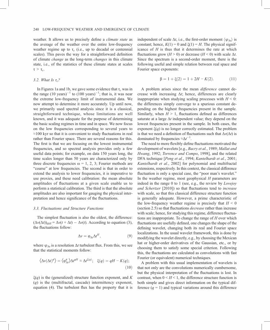
Figure 5. A comparison of the different structure function analyses(root-mean-square (RMS)) applied to the ensemble of three monthlysurface series discussed in section 3.4 (NASA GISS, NOAANCDC, and HadCRUT3), each globally averaged, from 1881 to2008 (1548 points each). The usual (difference, poor man’s) (bot-tom left) structure function (thin gray), (bottom right) the tendencystructure function (thin gray), the maximum of the two (“Hybrid,”thick, gray), and the Haar (in black) are shown. The latter has beenincreased by a factor C = 100.35 = 2.2; the resulting RMS deviationwith respect to the hybrid is ±14%. Reference slopes with exponentsξ(2)/2 ≈ 0.4 and �0.1 are also shown (corresponding to spectralexponents β = 1 + ξ(2) = 1.8 and 0.8, respectively). In terms ofdifference fluctuations, we can use the global RMS hΔT(Δt)2i1/2annual structure functions (fitted for 129 years > Δt > 10 years),obtaining hΔT(Δt)2i1/2 ≈ 0.08Δt0.33 for the ensemble. In comparison,Lovejoy and Schertzer [1986] found the very similar hΔT(Δt)2i1/2 ≈0.077Δt0.4 using Northern Hemisphere data (these correspond toβc = 1.66 and 1.8, respectively).
242 LOW-FREQUENCY WEATHER AND EMERGENCE OF CLIMATE
2° � 2°) [Hansen et al., 2010], and the HadCRUT3 data set(from 1850 to 2010 on a 5° � 5° grid). HadCRUT3 is amerged product created out of the Climate Research UnitHadSST2 [Rayner et al., 2006] SST data set and its compan-ion data set CRUTEM3 of atmospheric temperatures overland. The NOAA NCDC and NASA GISS are both heavilybased on the Global Historical Climatology Network [Peter-son and Vose, 1997] and have many similarities including theuse of sophisticated statistical methods to smooth and reducenoise. In contrast, the HadCRUTM3 data is less processed.Unsurprisingly, these series are quite similar, although anal-ysis of the scale by scale differences between the spectra isinteresting [see Lovejoy and Schertzer, 2012].Each grid point in each data set suffered from missing data
points so that here we consider the globally averaged seriesobtained by averaging over all the available data for thecommon 129 year period 1880–2008. Before analysis, eachseries was periodically detrended to remove the annual cycle;if this is not done, then the scaling near Δt ≈ 1 year will beartificially degraded. The detrending was done by setting theamplitudes of the Fourier components corresponding to an-nual periods to the “background” spectral values.Figure 5 shows the comparison of the difference, ten-
dency, hybrid, and Haar root-mean-square (RMS) structurefunctions hΔT(Δt)2i1/2, the latter increased by a factor C =100.35 ≈ 2.2. Before commenting on the physical implica-tions, let us first make some technical remarks. It can beseen that the “calibrated” Haar and hybrid structure func-tions are very close; the deviations are ±14% over theentire range of nearly a factor 103 in Δt. This implies thatthe indicated amplitude scale of the calibrated Haar struc-ture function in degrees K is quite accurate and that to agood approximation, the Haar structure function can pre-serve the simple interpretation of the difference and ten-dency structure functions: in regions where the logarithmicslope is between �1 and 0, it approximates the tendencystructure function, whereas in regions where the logarith-mic slope is between 0 and 1, the calibrated Haar structurefunction approximates the difference structure function. Forexample, from the graph, we can see that global-scaletemperature fluctuations decrease from ≈0.3 K at monthlyscales, to ≈0.2 K at 10 years and then increase to ≈0.8 K at≈100 years. All of the numbers have obvious implications,although note that they indicate the mean overall range ofthe fluctuations so that, for example, the 0.8 K correspondsto ±0.4 K, etc.From Figure 5, we also see that the global surface tempera-
tures separate into two regimes at about τc ≈ 10 years, withnegative and positive logarithmic slopes = ξ(2)/2 ≈�0.1, 0.4for Δt < τc, and Δt > τc, respectively. Since β = 1 + ξ(2)(equation (11)), we have β ≈ 0.8, 1.8. We also analyzed the
first-order structure function whose exponent ξ(1) = H; atthese scales, the intermittency (K(2), equation (4)) ≈ 0.03 sothat ξ(2) ≈ 2H so that H ≈ �0.1, 0.4 confirming that fluctua-tions decreasewith scale in the low-frequencyweather regimebut increase again at lower frequencies in the climate regime(more precise intermittency analyses are given in the work ofLovejoy and Schertzer [2012]). Note that ignoring intermit-tency, the critical value of β discriminating between growingand decreasing fluctuations (i.e., H < 0, H > 0) is β = 1.Before pursuing the Haar structure function, let us briefly
consider its sensitivity to nonscaling perturbations, i.e.,to nonscaling external trends superposed on the data, whichbreak the overall scaling. Even when there is no particularreason to suspect such trends, the desire to filter them out iscommonly invoked to justify the use of special wavelets, ornearly equivalently, of various orders of the multifractal de-trended fluctuation analysis technique (MFDFA) [Kantelhardt
LOVEJOY AND SCHERTZER 243
et al., 2002]. A simple way to produce a higher-order Haarwavelet that eliminates polynomials of order n is simply toiterate (n + 1 times) the difference operator in equation(14). For example, iterating it three times yields the “qua-
dratic Haar” fluctuation ðΔvðΔtÞÞHaarquad ¼3
Δtðsðt þ ΔtÞ −
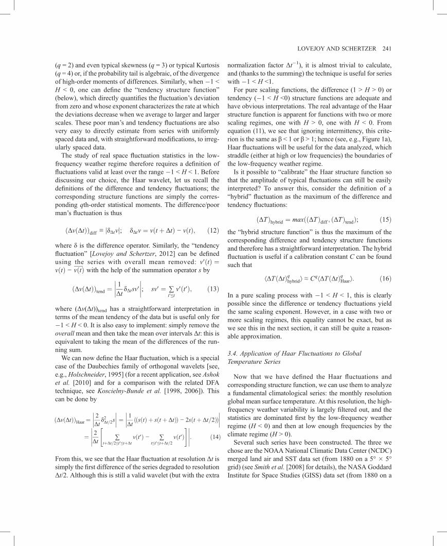
3sðt þ Δt=3Þþ 3sðt − Δt=3Þ − sðt − ΔtÞÞ. This fluctuation issensitive to structures of size Δt�1 and, hence, useful overthe range �1 < H < 2, and it is blind to polynomials oforder 1 (lines). In comparison, the nth-order DFA techniquedefines fluctuations using the RMS deviations of thesummed series s(t) from regressions of nth-order polyno-mials so that quadratic Haar fluctuations are nearly equiva-lent to the quadratic MFDFA RMS deviations (althoughthese deviations are not strictly wavelets, note that theMFDFA uses a scaling function ≈ Δv Δt; hence, with DFAexponent, αDFA = 1 + H). Although at first sight the insen-sitivity of these higher-order wavelets to trends may seemadvantageous, it should be recalled that, on the one hand,they only filter out polynomial trends (and not, for example,the more geophysically relevant periodic trends), while onthe other hand, even for this, they are “overkill” since thetrends they filter are filtered at all scales, not just the largest.Indeed, if one suspects the presence of external polynomialtrends, it suffices to eliminate them over the whole series(i.e., at the largest scales) and then to analyze the resultingdeviations using the Haar fluctuations.Figure 6 shows the usual (linear) Haar RMS structure
function (equation (14)) compared to the quadratic Haar andquadratic MFDFA structure functions. Unsurprisingly, thelatter two are close to each other (after applying differentcalibration constants, see the figure caption), that the low and
Figure 6. Same temperature data as Figure 5: a comparison of theRMS Haar structure function (multiplied by 100.35 = 2.2), the RMSquadratic Haar (multiplied by 100.15 = 1.4), and the RMS quadraticmultifractal detrended fluctuation analysis (multiplied by 101.5 =31.6).
high-frequency exponents are roughly the same. However,the transition point has shifted by nearly a factor of 3 so that,overall, they are rather different from the Haar structurefunction, and it is clearly not possible to simultaneously“calibrate” the high- and low-frequency parts. The drawbackwith these higher-order fluctuations is thus that we lose thesimplicity of interpretation of the Haar wavelet, and unlessH > 1, we obtain no obvious advantage.
4. THE TRANSITION FROM LOW-FREQUENCYWEATHER TO THE CLIMATE
4.1. Intermediate-Scale Multiproxy Series
In section 2, we discussed atmospheric variability overthe frustratingly short instrumentally accessible range oftime scales (roughly Δt < 150 years) and saw evidence thatweakly variable low-frequency weather gives way to a newhighly variable climate regime at a scale τc, somewhere inthe range 10–30 years. In Figure 1a, we already glimpsedthe much longer 1–100 kyr scales accessible primarily viaice core paleotemperatures (see also below); these confirmedthat, at least when averaged over the last 100 kyr or so, theclimate does indeed have a new scaling regime with fluctua-tions increasing rather than decreasing in amplitude withscale (H > 0).Since the temporal resolution of the high-resolution Green-
land Ice Core Project (GRIP) paleotemperatures was ≈ 5.2years (and for the Vostok series ≈100 years), these paleotem-perature resolutions do not greatly overlap the instrumentalrange; it is thus useful to consider other intermediates: the“multiproxy” series that have been developed following thework of Mann et al. [1998]. Another reason to use interme-diate-scale data is because we are living in a climate epoch,which is exceptional in both its long- and short-term aspects.For example, consider the long stretch of relatively mild andstable conditions since the retreat of the last ice sheets about11.5 kyr ago, the “Holocene.” This epoch is claimed to be atleast somewhat exceptional: it has even been suggested thatsuch stability is a precondition for the invention of farmingand thus for civilization itself [Petit et al., 1999]. It is there-fore possible that the paleoclimate statistics averaged overseries 100 kyr or longer may not be as pertinent as we wouldlike for understanding the current epoch. Similarly, at thehigh-frequency end of the spectrum, there is the issue of“twentieth century exceptionalism,” a consequence of twen-tieth century warming and the probability that at least someof it is of anthropogenic, not natural origin. Since these affecta large part of the instrumental record, it is problematic to usethe latter as the basis for extrapolations to centennial andmillennial scales. In the following, we try to assess both
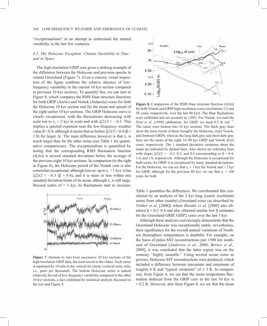
Figure 8. Comparison of the RMS Haar structure function (S(Δt))for both Vostok and GRIP high-resolution cores (resolutions 5.2 and50 years, respectively, over the last 90 kyr). The Haar fluctuationswere calibrated and are accurate to ±20%. For Vostok, we used thePetit et al. [1999] calibration; for GRIP, we used 0.5 K mil�1.The series were broken into 10 kyr sections. The thick gray linesshow the most recent of these (roughly the Holocene, (top) Vostok,and (bottom) GRIP), whereas the long dark gray and short dark graylines are the mean of the eight 10–90 kyr GRIP and Vostok S(Δt)cores, respectively. The 1 standard deviation variations about themean are indicated by dashed lines. Also shown are reference lineswith slopes ξ(2)/2 = �0.3, 0.2, and 0.4 corresponding to β = 0.4,1.4, and 1.8, respectively. Although the Holocene is exceptional forboth series, for GRIP, it is exceptional by many standard deviations.For the Holocene, we can see that τc ≈ 1 kyr for Vostok and ≈ 2 kyrfor GRIP, although for the previous 80 kyr, we see that τc ≈ 100years for both.
244 LOW-FREQUENCY WEATHER AND EMERGENCE OF CLIMATE
“exceptionalisms” in an attempt to understand the naturalvariability in the last few centuries.
4.2. The Holocene Exception: Climate Variability in Timeand in Space
The high-resolution GRIP core gives a striking example ofthe difference between the Holocene and previous epochs incentral Greenland (Figure 7). Even a cursory visual inspec-tion of the figure confirms the relative absence of low-frequency variability in the current 10 kyr section comparedto previous 10 kyr sections. To quantify this, we can turn toFigure 8, which compares the RMS Haar structure functionsfor both GRIP (Arctic) and Vostok (Antarctic) cores for boththe Holocene 10 kyr section and for the mean and spread ofthe eight earlier 10 kyr sections. The GRIP Holocene curve isclearly exceptional, with the fluctuations decreasing withscale out to τc ≈ 2 kyr in scale and with ξ(2)/2 ≈ �0.3. Thisimplies a spectral exponent near the low-frequency weathervalue β ≈ 0.4, although it seems that as before ξ(2)/2 ≈ 0.4 (β ≈1.8) for larger Δt. The main difference however is that τc ismuch larger than for the other series (see Table 1 for quanti-tative comparisons). The exceptionalism is quantified bynoting that the corresponding RMS fluctuation function(S(Δt)) is several standard deviations below the average ofthe previous eight 10 kyr sections. In comparison (to the rightin Figure 8), the Holocene period of the Vostok core is alsosomewhat exceptional, although less so: up to τc ≈ 1 kyr, it hasξ(2)/2 ≈ �0.3 (β ≈ 0.4), and it is more or less within onestandard deviation limits of its mean, although τc is still large.Beyond scales of ≈ 1 kyr, its fluctuations start to increase;
Figure 7. (bottom to top) Four successive 10 kyr sections of thehigh-resolution GRIP data, the most recent to the oldest. Each seriesis separated by 10 mils in the vertical for clarity (vertical units, mils,i.e., parts per thousand). The bottom Holocene series is indeedrelatively devoid of low-frequency variability compared to the other10 kyr sections, a fact confirmed by statistical analysis discussed inthe text and Figure 8.
Table 1 quantifies the differences. We corroborated this con-clusion by an analysis of the 2 kyr long (yearly resolution)series from other (nearby) Greenland cores (as described byVinther et al. [2008]) where Blender et al. [2006] also ob-tained β ≈ 0.2–0.4 and also obtained similar low β estimatesfor the Greenland GRIP, GISP2 cores over the last 3 kyr.Although these analyses convincingly demonstrate that the
Greenland Holocene was exceptionally stable, nevertheless,their significance for the overall natural variations of North-ern Hemisphere temperatures is doubtful. For example, onthe basis of paleo-SST reconstructions just 1500 km south-east of Greenland [Andersen et al., 2004; Berner et al.,2008], it was concluded that the latter region was on thecontrary “highly unstable.” Using several ocean cores asproxies, Holocene SST reconstructions were produced, whichincluded a difference between maximum and minimum ofroughly 6 K and “typical variations” of 1–3 K. In compari-son, from Figure 8, we see that the mean temperature fluc-tuation deduced from the GRIP core in the last 10 kyr is≈ 0.2 K. However, also from Figure 8, we see that the mean
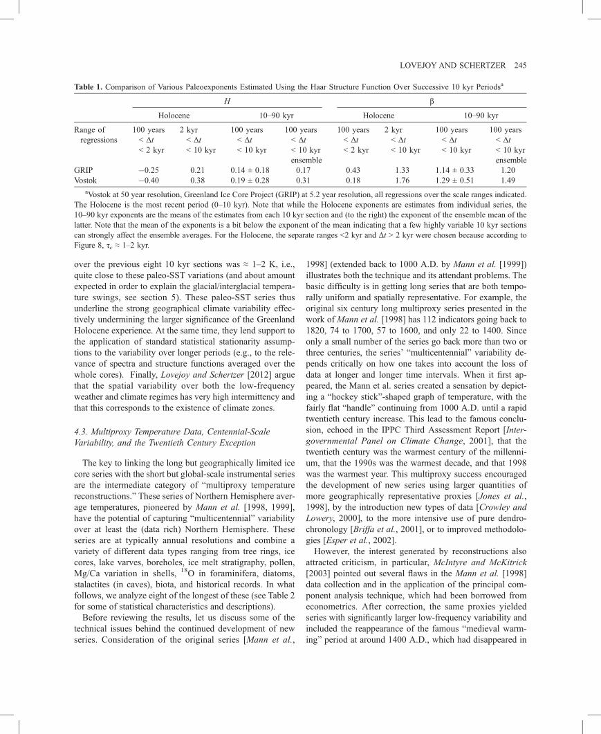
Table 1. Comparison of Various Paleoexponents Estimated Using the Haar Structure Function Over Successive 10 kyr Periodsa
H β
Holocene 10–90 kyr Holocene 10–90 kyr
Range ofregressions
100 years< Δt< 2 kyr
2 kyr< Δt< 10 kyr
100 years< Δt< 10 kyr
100 years< Δt< 10 kyrensemble
100 years< Δt< 2 kyr
2 kyr< Δt< 10 kyr
100 years< Δt< 10 kyr
100 years< Δt< 10 kyrensemble
GRIP �0.25 0.21 0.14 ± 0.18 0.17 0.43 1.33 1.14 ± 0.33 1.20Vostok �0.40 0.38 0.19 ± 0.28 0.31 0.18 1.76 1.29 ± 0.51 1.49
aVostok at 50 year resolution, Greenland Ice Core Project (GRIP) at 5.2 year resolution, all regressions over the scale ranges indicated.The Holocene is the most recent period (0–10 kyr). Note that while the Holocene exponents are estimates from individual series, the10–90 kyr exponents are the means of the estimates from each 10 kyr section and (to the right) the exponent of the ensemble mean of thelatter. Note that the mean of the exponents is a bit below the exponent of the mean indicating that a few highly variable 10 kyr sectionscan strongly affect the ensemble averages. For the Holocene, the separate ranges <2 kyr and Δt > 2 kyr were chosen because according toFigure 8, τc ≈ 1–2 kyr.
LOVEJOY AND SCHERTZER 245
over the previous eight 10 kyr sections was ≈ 1–2 K, i.e.,quite close to these paleo-SST variations (and about amountexpected in order to explain the glacial/interglacial tempera-ture swings, see section 5). These paleo-SST series thusunderline the strong geographical climate variability effec-tively undermining the larger significance of the GreenlandHolocene experience. At the same time, they lend support tothe application of standard statistical stationarity assump-tions to the variability over longer periods (e.g., to the rele-vance of spectra and structure functions averaged over thewhole cores). Finally, Lovejoy and Schertzer [2012] arguethat the spatial variability over both the low-frequencyweather and climate regimes has very high intermittency andthat this corresponds to the existence of climate zones.
4.3. Multiproxy Temperature Data, Centennial-ScaleVariability, and the Twentieth Century Exception
The key to linking the long but geographically limited icecore series with the short but global-scale instrumental seriesare the intermediate category of “multiproxy temperaturereconstructions.” These series of Northern Hemisphere aver-age temperatures, pioneered by Mann et al. [1998, 1999],have the potential of capturing “multicentennial” variabilityover at least the (data rich) Northern Hemisphere. Theseseries are at typically annual resolutions and combine avariety of different data types ranging from tree rings, icecores, lake varves, boreholes, ice melt stratigraphy, pollen,Mg/Ca variation in shells, 18O in foraminifera, diatoms,stalactites (in caves), biota, and historical records. In whatfollows, we analyze eight of the longest of these (see Table 2for some of statistical characteristics and descriptions).Before reviewing the results, let us discuss some of the
technical issues behind the continued development of newseries. Consideration of the original series [Mann et al.,
1998] (extended back to 1000 A.D. by Mann et al. [1999])illustrates both the technique and its attendant problems. Thebasic difficulty is in getting long series that are both tempo-rally uniform and spatially representative. For example, theoriginal six century long multiproxy series presented in thework of Mann et al. [1998] has 112 indicators going back to1820, 74 to 1700, 57 to 1600, and only 22 to 1400. Sinceonly a small number of the series go back more than two orthree centuries, the series’ “multicentennial” variability de-pends critically on how one takes into account the loss ofdata at longer and longer time intervals. When it first ap-peared, the Mann et al. series created a sensation by depict-ing a “hockey stick”-shaped graph of temperature, with thefairly flat “handle” continuing from 1000 A.D. until a rapidtwentieth century increase. This lead to the famous conclu-sion, echoed in the IPPC Third Assessment Report [Inter-governmental Panel on Climate Change, 2001], that thetwentieth century was the warmest century of the millenni-um, that the 1990s was the warmest decade, and that 1998was the warmest year. This multiproxy success encouragedthe development of new series using larger quantities ofmore geographically representative proxies [Jones et al.,1998], by the introduction new types of data [Crowley andLowery, 2000], to the more intensive use of pure dendro-chronology [Briffa et al., 2001], or to improved methodolo-gies [Esper et al., 2002].However, the interest generated by reconstructions also
attracted criticism, in particular, McIntyre and McKitrick[2003] pointed out several flaws in the Mann et al. [1998]data collection and in the application of the principal com-ponent analysis technique, which had been borrowed fromeconometrics. After correction, the same proxies yieldedseries with significantly larger low-frequency variability andincluded the reappearance of the famous “medieval warm-ing” period at around 1400 A.D., which had disappeared in
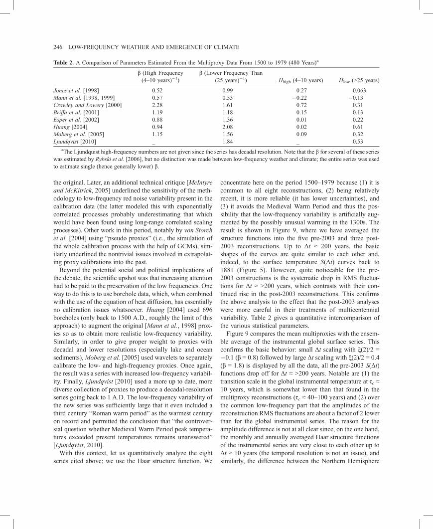
Table 2. A Comparison of Parameters Estimated From the Multiproxy Data From 1500 to 1979 (480 Years)a
β (High Frequency(4–10 years)�1)
β (Lower Frequency Than(25 years)�1) Hhigh (4–10 years) Hlow (>25 years)
Jones et al. [1998] 0.52 0.99 �0.27 0.063Mann et al. [1998, 1999] 0.57 0.53 �0.22 �0.13Crowley and Lowery [2000] 2.28 1.61 0.72 0.31Briffa et al. [2001] 1.19 1.18 0.15 0.13Esper et al. [2002] 0.88 1.36 0.01 0.22Huang [2004] 0.94 2.08 0.02 0.61Moberg et al. [2005] 1.15 1.56 0.09 0.32Ljundqvist [2010] _ 1.84 _ 0.53
aThe Ljundquist high-frequency numbers are not given since the series has decadal resolution. Note that the β for several of these serieswas estimated by Rybski et al. [2006], but no distinction was made between low-frequency weather and climate; the entire series was usedto estimate single (hence generally lower) β.
246 LOW-FREQUENCY WEATHER AND EMERGENCE OF CLIMATE
the original. Later, an additional technical critique [McIntyreand McKitrick, 2005] underlined the sensitivity of the meth-odology to low-frequency red noise variability present in thecalibration data (the latter modeled this with exponentiallycorrelated processes probably underestimating that whichwould have been found using long-range correlated scalingprocesses). Other work in this period, notably by von Storchet al. [2004] using “pseudo proxies” (i.e., the simulation ofthe whole calibration process with the help of GCMs), sim-ilarly underlined the nontrivial issues involved in extrapolat-ing proxy calibrations into the past.Beyond the potential social and political implications of
the debate, the scientific upshot was that increasing attentionhad to be paid to the preservation of the low frequencies. Oneway to do this is to use borehole data, which, when combinedwith the use of the equation of heat diffusion, has essentiallyno calibration issues whatsoever. Huang [2004] used 696boreholes (only back to 1500 A.D., roughly the limit of thisapproach) to augment the original [Mann et al., 1998] prox-ies so as to obtain more realistic low-frequency variability.Similarly, in order to give proper weight to proxies withdecadal and lower resolutions (especially lake and oceansediments), Moberg et al. [2005] used wavelets to separatelycalibrate the low- and high-frequency proxies. Once again,the result was a series with increased low-frequency variabil-ity. Finally, Ljundqvist [2010] used a more up to date, morediverse collection of proxies to produce a decadal-resolutionseries going back to 1 A.D. The low-frequency variability ofthe new series was sufficiently large that it even included athird century “Roman warm period” as the warmest centuryon record and permitted the conclusion that “the controver-sial question whether Medieval Warm Period peak tempera-tures exceeded present temperatures remains unanswered”[Ljundqvist, 2010].With this context, let us quantitatively analyze the eight
series cited above; we use the Haar structure function. We
concentrate here on the period 1500–1979 because (1) it iscommon to all eight reconstructions, (2) being relativelyrecent, it is more reliable (it has lower uncertainties), and(3) it avoids the Medieval Warm Period and thus the pos-sibility that the low-frequency variability is artificially aug-mented by the possibly unusual warming in the 1300s. Theresult is shown in Figure 9, where we have averaged thestructure functions into the five pre-2003 and three post-2003 reconstructions. Up to Δt ≈ 200 years, the basicshapes of the curves are quite similar to each other and,indeed, to the surface temperature S(Δt) curves back to1881 (Figure 5). However, quite noticeable for the pre-2003 constructions is the systematic drop in RMS fluctua-tions for Δt ≈ >200 years, which contrasts with their con-tinued rise in the post-2003 reconstructions. This confirmsthe above analysis to the effect that the post-2003 analyseswere more careful in their treatments of multicentennialvariability. Table 2 gives a quantitative intercomparison ofthe various statistical parameters.Figure 9 compares the mean multiproxies with the ensem-
ble average of the instrumental global surface series. Thisconfirms the basic behavior: small Δt scaling with ξ(2)/2 =�0.1 (β = 0.8) followed by large Δt scaling with ξ(2)/2 = 0.4(β = 1.8) is displayed by all the data, all the pre-2003 S(Δt)functions drop off for Δt ≈ >200 years. Notable are (1) thetransition scale in the global instrumental temperature at τc ≈10 years, which is somewhat lower than that found in themultiproxy reconstructions (τc ≈ 40–100 years) and (2) overthe common low-frequency part that the amplitudes of thereconstruction RMS fluctuations are about a factor of 2 lowerthan for the global instrumental series. The reason for theamplitude difference is not at all clear since, on the one hand,the monthly and annually averaged Haar structure functionsof the instrumental series are very close to each other up toΔt ≈ 10 years (the temporal resolution is not an issue), andsimilarly, the difference between the Northern Hemisphere
Figure 9. (bottom) RMS Haar fluctuation for the mean of the pre-2003 and post-2003 series from 1500 to 1979 (solid black and graycurves, respectively, and excluding the Crowley series due to itspoor resolution), along with (top) the mean of the globally averagedmonthly resolution surface series from Figure 5 (solid gray). Inorder to assess the effect of the twentieth century warming, thestructure functions for the multiproxy data were recalculated from1500 to 1900 only (the associated thin dashed lines) and for theinstrumental surface series with their linear trends from 1880 to2008 removed (the data from 1880 to 1899 are too short to yield ameaningful S(Δt) estimate for the lower frequencies of interest).While the large Δt variability is reduced a little, the basic power lawtrend is robust, especially for the post-2003 reconstructions. Notethat the decrease in S(Δt) for the linearly detrended surface seriesover the last factor of 2 or so in lag Δt is a pure artifact of thedetrending. We may conclude that the low-frequency rise is not anartifact of an external linear trend. Reference lines corresponding toβ = 0.8 and 1.8 have been added.
Figure 10. (bottom left) RMS Haar fluctuations for the meanmonthly, global surface series (thin gray, from Figure 5) and (bot-tom right) the mean pre-2003 (medium gray) and (bottom middle)mean post-2003 proxies (dark gray, from Figure 9) as well as themean (top right) Vostok S(Δt) function over the last 420 kyr inter-polated to 300 year resolution and using the Petit et al. [1999]calibration. Also shown (the rectangle) is the “interglacial window,”the probable typical range of fluctuations and quasiperiods of theglacial-interglacials. The “calibration” of the fluctuation amplitudesis accurate to ±25%.
LOVEJOY AND SCHERTZER 247
and the Southern Hemisphere instrumental S(Δt) functions ismuch smaller than this (only about ≈15%).To get another perspective on this low-frequency variabil-
ity, we can compare the instrumental and multiproxy struc-ture functions with those from ice core paleotemperaturediscussed in more detail in the next section. In Figure 10, wehave superposed the calibrated deuterium-based RMS tem-perature fluctuations with RMSmultiproxy and RMS surfaceseries fluctuations (we return to this in section 5). We see thatextrapolating the latter out to 30–50 kyr is quite compatiblewith the Vostok core with the “interglacial window” (i.e., therough quasiperiod and amplitude corresponding to the inter-glacials). Although the Vostok S(Δt) curve is from the entire420 kyr record (not just the Holocene), this certainly makes itplausible that while the surface series appear to have realisticlow-frequency variability, the variability of the reconstruc-tions is too small (although the post-2003 reconstructions are
indeed more realistic than the contrasting relative lack ofvariability in the pre-2003 reconstructions).
4.4. Twentieth Century Exceptionalism
Although the reconstructions and instrumental series qual-itatively agree, their quantitative disagreement is large andrequires explanation. In this section, we consider whetherthis could be a consequence of the twentieth century “excep-tionalism” discussed earlier, the fact that, irrespective of thecause, the twentieth century is somewhat warmer than thenineteenth and earlier centuries. It has been recognized thatthis warming causes problems for the calibration of theproxies [e.g., Ljundqvist, 2010], and it will clearly contributeto the RMS multicennial variability in Figure 9. In order todemonstrate that the basic type of statistical variability is notan artifact of the inclusion of exceptional twentieth centurytemperatures in Figure 9, we also show the correspondingHaar structure functions for the earlier period 1500–1900.Truncating the instrumental series at 1900 would result in aseries only 20 years long; therefore, the closest equivalent forthe surface series was to remove overall linear trends andthen redo the analysis. As expected, the figure shows that allthe large Δt fluctuations are reduced but that the basic scalingbehaviors are apparently not affected. We conclude that boththe type of variability as characterized by the scaling expo-nents and the transition scale τc are fairly robust, if difficult,
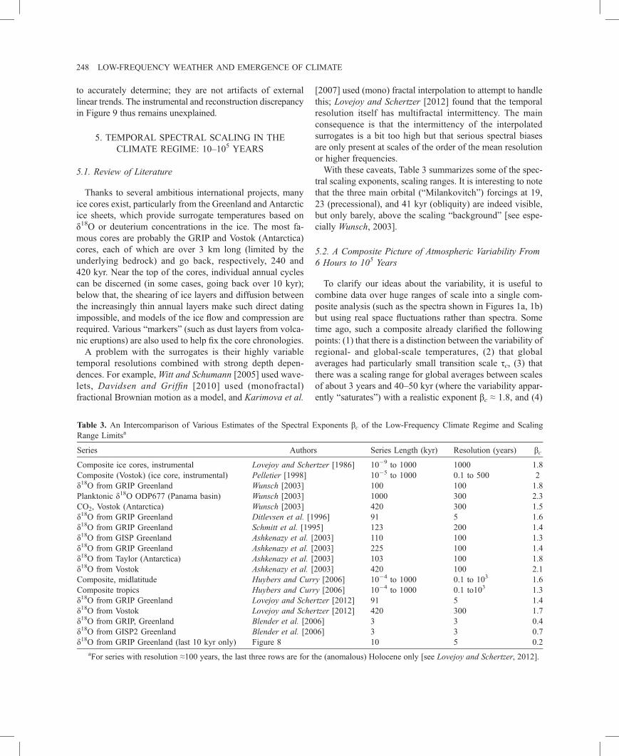
248 LOW-FREQUENCY WEATHER AND EMERGENCE OF CLIMATE
to accurately determine; they are not artifacts of externallinear trends. The instrumental and reconstruction discrepancyin Figure 9 thus remains unexplained.
5. TEMPORAL SPECTRAL SCALING IN THECLIMATE REGIME: 10–105 YEARS
5.1. Review of Literature
Thanks to several ambitious international projects, manyice cores exist, particularly from the Greenland and Antarcticice sheets, which provide surrogate temperatures based onδ18O or deuterium concentrations in the ice. The most fa-mous cores are probably the GRIP and Vostok (Antarctica)cores, each of which are over 3 km long (limited by theunderlying bedrock) and go back, respectively, 240 and420 kyr. Near the top of the cores, individual annual cyclescan be discerned (in some cases, going back over 10 kyr);below that, the shearing of ice layers and diffusion betweenthe increasingly thin annual layers make such direct datingimpossible, and models of the ice flow and compression arerequired. Various “markers” (such as dust layers from volca-nic eruptions) are also used to help fix the core chronologies.A problem with the surrogates is their highly variable
temporal resolutions combined with strong depth depen-dences. For example,Witt and Schumann [2005] used wave-lets, Davidsen and Griffin [2010] used (monofractal)fractional Brownian motion as a model, and Karimova et al.
able 3. An Intercomparison of Various Estimates of the Spectral Exponents βc of the Low-Frequency Climate Regime and Scalingange Limitsa
eries Authors Series Length (kyr) Resolution (years) βc
omposite ice cores, instrumental Lovejoy and Schertzer [1986] 10�9 to 1000 1000 1.8omposite (Vostok) (ice core, instrumental) Pelletier [1998] 10�5 to 1000 0.1 to 500 218O from GRIP Greenland Wunsch [2003] 100 100 1.8lanktonic δ18O ODP677 (Panama basin) Wunsch [2003] 1000 300 2.3O2, Vostok (Antarctica) Wunsch [2003] 420 300 1.518O from GRIP Greenland Ditlevsen et al. [1996] 91 5 1.618O from GRIP Greenland Schmitt et al. [1995] 123 200 1.418O from GISP Greenland Ashkenazy et al. [2003] 110 100 1.318O from GRIP Greenland Ashkenazy et al. [2003] 225 100 1.418O from Taylor (Antarctica) Ashkenazy et al. [2003] 103 100 1.818O from Vostok Ashkenazy et al. [2003] 420 100 2.1omposite, midlatitude Huybers and Curry [2006] 10�4 to 1000 0.1 to 103 1.6omposite tropics Huybers and Curry [2006] 10�4 to 1000 0.1 to103 1.318O from GRIP Greenland Lovejoy and Schertzer [2012] 91 5 1.418O from Vostok Lovejoy and Schertzer [2012] 420 300 1.718O from GRIP, Greenland Blender et al. [2006] 3 3 0.418O from GISP2 Greenland Blender et al. [2006] 3 3 0.718O from GRIP Greenland (last 10 kyr only) Figure 8 10 5 0.2
aFor series with resolution ≈100 years, the last three rows are for the (anomalous) Holocene only [see Lovejoy and Schertzer, 2012].
TR
S
CCδPCδδδδδδCCδδδδδ
[2007] used (mono) fractal interpolation to attempt to handlethis; Lovejoy and Schertzer [2012] found that the temporalresolution itself has multifractal intermittency. The mainconsequence is that the intermittency of the interpolatedsurrogates is a bit too high but that serious spectral biasesare only present at scales of the order of the mean resolutionor higher frequencies.With these caveats, Table 3 summarizes some of the spec-
tral scaling exponents, scaling ranges. It is interesting to notethat the three main orbital (“Milankovitch”) forcings at 19,23 (precessional), and 41 kyr (obliquity) are indeed visible,but only barely, above the scaling “background” [see espe-cially Wunsch, 2003].
5.2. A Composite Picture of Atmospheric Variability From6 Hours to 105 Years
To clarify our ideas about the variability, it is useful tocombine data over huge ranges of scale into a single com-posite analysis (such as the spectra shown in Figures 1a, 1b)but using real space fluctuations rather than spectra. Sometime ago, such a composite already clarified the followingpoints: (1) that there is a distinction between the variability ofregional- and global-scale temperatures, (2) that globalaverages had particularly small transition scale τc, (3) thatthere was a scaling range for global averages between scalesof about 3 years and 40–50 kyr (where the variability appar-ently “saturates”) with a realistic exponent βc ≈ 1.8, and (4)
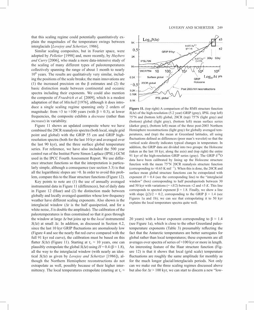
Figure 11. (top right) A comparison of the RMS structure functionS(Δt) of the high-resolution (5.2 year) GRIP (gray), IPSL (top left)75°N and (bottom left) global, 20CR (top) 75°N (light gray) and(bottom) global (light gray), (bottom left) mean surface series(darker gray), (bottom left) mean of the three post-2003 NorthernHemisphere reconstructions (light gray) for globally averaged tem-peratures, and (top) the mean at Greenland latitudes, all usingfluctuations defined as differences (poor man’s wavelet) so that thevertical scale directly indicates typical changes in temperature. Inaddition, the GRIP data are divided into two groups: the Holocene(taken as the last 10 kyr, along the axis) and (top right) the entire91 kyr of the high-resolution GRIP series (gray). The GRIP δ18Odata have been calibrated by lining up the Holocene structurefunction with the mean 75°N 20CR reanalysis structure function(corresponding to ≈0.65 K mil�1). When this is done, the 20CR andsurface mean global structure functions can be extrapolated withexponent H ≈ 0.4 (see the corresponding line) to the “interglacialwindow” (box) corresponding to half pseudoperiods between 30and 50 kyr with variations (= ±S/2) between ±2 and ±3 K. This linecorresponds to spectral exponent β = 1.8. Finally, we show a linewith slope ξ(2)/2 = 0.2, corresponding to the GRIP β = 1.4 (seeFigures 1a and 1b); we can see that extrapolating it to 50 kyrexplains the local temperature spectra quite well.
LOVEJOY AND SCHERTZER 249
that this scaling regime could potentially quantitatively ex-plain the magnitudes of the temperature swings betweeninterglacials [Lovejoy and Schertzer, 1986].Similar scaling composites, but in Fourier space, were
adopted by Pelletier [1998] and, more recently, by Huybersand Curry [2006], who made a more data-intensive study ofthe scaling of many different types of paleotemperaturescollectively spanning the range of about 1 month to nearly106 years. The results are qualitatively very similar, includ-ing the positions of the scale breaks; the main innovations are(1) the increased precision on the β estimates and (2) thebasic distinction made between continental and oceanicspectra including their exponents. We could also mentionthe composite of Fraedrich et al. [2009], which is a modestadaptation of that of Mitchell [1976], although it does intro-duce a single scaling regime spanning only 2 orders ofmagnitude: from ≈3 to ≈100 years (with β ≈ 0.3), at lowerfrequencies, the composite exhibits a decrease (rather thanincrease) in variability.Figure 11 shows an updated composite where we have
combined the 20CR reanalysis spectra (both local, single gridpoint and global) with the GRIP 55 cm and GRIP high-resolution spectra (both for the last 10 kyr and averaged overthe last 90 kyr), and the three surface global temperatureseries. For reference, we have also included the 500 yearcontrol run of the Institut Pierre Simon Laplace (IPSL) GCMused in the IPCC Fourth Assessment Report. We use differ-ence structure functions so that the interpretation is particu-larly simple, although a consequence (see section 3.3) is thatall the logarithmic slopes are >0. In order to avoid this prob-lem, compare this to the Haar structure functions (Figure 12).Key points to note are (1) the use of annually averaged
instrumental data in Figure 11 (differences), but of daily datain Figure 12 (Haar) and (2) the distinction made betweenglobally and locally averaged quantities whose low-frequencyweather have different scaling exponents. Also shown is theinterglacial window (Δt is the half quasiperiod, and for awhite noise, S is double the amplitude). The calibration of thepaleotemperatures is thus constrained so that it goes throughthe window at large Δt but joins up to the local instrumentalS(Δt) at small Δt. In addition, as discussed in Section 4.2,since the last 10 kyr GRIP fluctuations are anomalously low(Figure 4 and see the nearly flat red curve compared with thefull 91 kyr red curve), the calibration must be based on thisflatter S(Δt) (Figure 11). Starting at τc ≈ 10 years, one canplausibly extrapolate the global S(Δt) usingH = 0.4 (β ≈ 1.8),all the way to the interglacial window (with nearly an iden-tical S(Δt) as given by Lovejoy and Schertzer [1986]), al-though the Northern Hemisphere reconstructions do notextrapolate as well, possibly because of their higher inter-mittency. The local temperatures extrapolate (starting at τc ≈
20 years) with a lower exponent corresponding to β ≈ 1.4(see Figure 1a), which is close to the other Greenland paleo-temperature exponents (Table 3) presumably reflecting thefact that the Antarctic temperatures are better surrogates forglobal rather than local temperatures; these exponents are allaverages over spectra of series of ≈100 kyr or more in length.An interesting feature of the Haar structure function (Fig-ure 12) is that it shows that local (grid scale) temperaturefluctuations are roughly the same amplitude for monthly asfor the much longer glacial/interglacials periods. Not onlycan we make out the three scaling regimes discussed abovebut also for Δt > 100 kyr, we can start to discern a new “low-
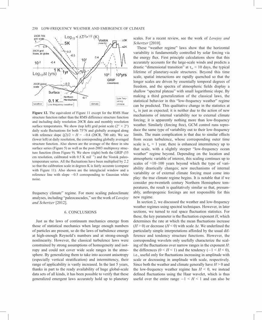
Figure 12. The equivalent of Figure 11 except for the RMS Haarstructure function rather than the RMS difference structure functionand including daily resolution 20CR data and monthly resolutionsurface temperatures. We show (top left) grid point scale (2° � 2°)daily scale fluctuations for both 75°N and globally averaged alongwith reference slope ξ(2)/2 ≈ H = �0.4 (20CR, 700 mb). We see(lower left) at daily resolution, the corresponding globally averagedstructure function. Also shown are the average of the three in situsurface series (Figure 5) as well as the post-2003 multiproxy struc-ture function (from Figure 9). We show (right) both the GRIP (55cm resolution, calibrated with 0.5 K mil�1) and the Vostok paleo-temperature series. All the fluctuations have been multiplied by 2.2so that the calibration scale in degrees K is fairly accurate (comparewith Figure 11). Also shown are the interglacial window and areference line with slope �0.5 corresponding to Gaussian whitenoise.
250 LOW-FREQUENCY WEATHER AND EMERGENCE OF CLIMATE
frequency climate” regime. For more scaling paleoclimateanalyses, including “paleocascades,” see the work of Lovejoyand Schertzer [2012].
6. CONCLUSIONS
Just as the laws of continuum mechanics emerge fromthose of statistical mechanics when large enough numbersof particles are present, so do the laws of turbulence emergeat high-enough Reynold’s numbers and at strong-enoughnonlinearity. However, the classical turbulence laws wereconstrained by strong assumptions of homogeneity and isot-ropy and could not cover wide scale ranges in the atmo-sphere. By generalizing them to take into account anisotropy(especially vertical stratification) and intermittency, theirrange of applicability is vastly increased. In the last 5 years,thanks in part to the ready availability of huge global-scaledata sets of all kinds, it has been possible to verify that thesegeneralized emergent laws accurately hold up to planetary
scales. For a recent review, see the work of Lovejoy andSchertzer [2010].These “weather regime” laws show that the horizontal
variability is fundamentally controlled by solar forcing viathe energy flux. First principle calculations show that thisaccurately accounts for the large-scale winds and predicts adrastic “dimensional transition” at τw ≈ 10 days, the typicallifetime of planetary-scale structures. Beyond this timescale, spatial interactions are rapidly quenched so that thelonger scales are driven by essentially temporal degrees offreedom, and the spectra of atmospheric fields display ashallow “spectral plateau” with small logarithmic slope. Bymaking a third generalization of the classical laws, thestatistical behavior in this “low-frequency weather” regimecan be predicted. This qualitative change in the statistics atτw is just as expected; it is neither due to the action of newmechanisms of internal variability nor to external climateforcing; it is apparently nothing more than low-frequencyweather. Similarly (forcing free), GCM control runs repro-duce the same type of variability out to their low-frequencylimits. The main complication is that due to similar effectsfrom ocean turbulence, whose corresponding outer timescale is τo ≈ 1 year, there is enhanced intermittency up tothat scale, with a slightly steeper “low-frequency oceanweather” regime beyond. Depending on the location andatmospheric variable of interest, this scaling continues up toscales of ≈10–100 years beyond which the type of vari-ability drastically changes; new mechanisms of internalvariability or of external climate forcing must come intoplay: the true climate regime begins. It is notable that if weconsider pre-twentieth century Northern Hemisphere tem-peratures, the result is qualitatively similar so that, presum-ably, anthropogenic forcings are not responsible for thisnew regime.In section 2, we discussed the weather and low-frequency
weather regimes using spectral techniques. However, in latersections, we turned to real space fluctuation statistics. Forthese, the key parameter is the fluctuation exponent H, whichdetermines the rate at which the mean fluctuations increase(H > 0) or decrease (H < 0) with scale Δt. We underlined theparticularly simple interpretations afforded by the usual dif-ference and tendency structure functions. However, thecorresponding wavelets only usefully characterize the scal-ing of the fluctuations over narrow ranges in the exponent H:the differences (0 < H < 1) and the tendency (�1 < H < 0),i.e., useful only for fluctuations increasing in amplitude withscale or decreasing in amplitude with scale, respectively.Since both the weather and climate generally have H > 0 andthe low-frequency weather regime has H < 0, we insteaddefined fluctuations using the Haar wavelet, which is thususeful over the entire range �1 < H < 1 and can also be
LOVEJOY AND SCHERTZER 251
“calibrated” to directly yield fluctuation amplitudes and canbe easily implemented numerically.In order to evaluate the statistical variability of the atmo-
sphere over as wide a range as possible, we combined theHaar wavelet with temperature data from the 20CR (1871–2008), (2° � 2°, 6 hourly), three surface series (5° � 5°,monthly), eight intermediate-length resolution “multiproxy”series of the Northern Hemisphere from 1500 to 1980 (yearly),and GRIP and Vostok paleotemperatures at 5.2 and ≈100 yearresolutions over lengths 91 and 420 kyr. The basic findingswere that the key transition scale τc from low-frequencyweather to climate, was somewhat variable, depending onthe field and geographical location. For example, for surfaceglobal temperatures, we found τc ≈ 10 years, whereas for themore reliable post-2003 Northern Hemisphere reconstruc-tions, τc ≈ 30 years, for the Holocene GRIP (Greenland)core, τc ≈ 2 kyr, the Holocene Vostok (Antarctica) core,τc ≈ 1 kyr, and the mean pre-Holocene paleotemperaturevalue, τc ≈ 100 years. We also found Hlw ≈ �0.4 and �0.1for local (e.g., 2° � 2° resolution) and global series, respec-tively, and Hc ≈ 0.4; although the GRIP value was a littlelower, these values correspond to βlw ≈ 0.2, 0.8, 1.8, respec-tively (ignoring intermittency corrections K(2), which rangedfrom Klw(2) ≈ 0.05 to Kc(2) ≈ 0.1; a full characterization ofthe intermittency, i.e., K(q) was been performed but was notdiscussed here).Although this basic overall three-scaling regime picture is
25 years old, much has changed to make it more convincing.Obviously, an important element is the improvement in thequantity and quality of the data, but we have also benefitedfrom advances in nonlinear dynamics as well as in dataanalysis techniques. In combination, these advances makethe model a seductive framework for understanding atmo-spheric variability over huge ranges of space-time scales. Itallows us to finally clarify the distinction between weather,its straightforward extension, without new elements, to low-frequency weather, and finally to the climate regime. Itallows for objective definitions of the weather (scales <τw),climate states (averages up to τc), and hence of climatechange (scales >τc). This new understanding of atmosphericvariability is essential for evaluating the realism of bothatmospheric and climate models. In particular, since withoutspecial external forcing, GCMs only model low-frequencyweather, the question is posed as to what types of externalforcing are required so that the GCM variability makes atransition to the climate regime with realistic scaling expo-nents and at a realistic time scales.
Acknowledgments.We thank P. Ditlevsen for providing the high-resolution GRIP data and A. Bunde for useful editorial and scien-tific comments.
REFERENCES
Andersen, C., N. Ko, and M. Moros (2004), A highly unstableHolocene climate in the subpolar North Atlantic: Evidence fromdiatoms, Quat. Sci. Rev., 23, 2155–2166.
Ashkenazy, Y., D. R. Baker, H. Gildor, and S. Havlin (2003),Nonlinearity and multifractality of climate change in the past420,000 years, Geophys. Res. Lett., 30(22), 2146, doi:10.1029/2003GL018099.
Ashok, V., T. Balakumaran, C. Gowrishankar, I. L. A. Vennila, andA. Nirmalkumar (2010), The fast Haar wavelet transform forsignal and image processing, Int. J. Comput. Sci. Inf. Security,7, 126–130.
Bacry, A., A. Arneodo, U. Frisch, Y. Gagne, and E. Hopfinger(1989), Wavelet analysis of fully developed turbulence data andmeasurement of scaling exponents, in Turbulence and CoherentStructures, edited by M. Lessieur and O. Metais, pp. 703–718,Kluwer Acad., Dordrecht, Netherlands.
Berner, K. S., N. Koç, D. Divine, F. Godtliebsen, and M. Moros(2008), A decadal-scale Holocene sea surface temperature recordfrom the subpolar North Atlantic constructed using diatoms andstatistics and its relation to other climate parameters, Paleocea-nography, 23, PA2210, doi:10.1029/2006PA001339.
Blender, R., and K. Fraedrich (2003), Long time memory in globalwarming simulations, Geophys. Res. Lett., 30(14), 1769, doi:10.1029/2003GL017666.
Blender, R., K. Fraedrich, and B. Hunt (2006), Millennial climatevariability: GCM-simulation and Greenland ice cores, Geophys.Res. Lett., 33, L04710, doi:10.1029/2005GL024919.
Bolgiano, R., Jr. (1959), Turbulent spectra in a stably stratifiedatmosphere, J. Geophys. Res., 64(12), 2226–2229.
Briffa, K., T. Osborn, F. Schweingruber, I. Harris, P. Jones, S.Shiyatov, and E. Vaganov (2001), Low-frequency temperaturevariations from a northern tree ring density network, J. Geophys.Res., 106(D3), 2929–2941.
Brunt, D. (1939), Physical and Dynamical Meteorology, 2nd ed.,454 pp., Cambridge Univ. Press, New York.
Bunde, A., J. F. Eichner, S. Havlin, E. Koscielny-Bunde, H. J.Schellnhuber, and D. Vyushin (2004), Comment on “Scaling ofatmosphere and ocean temperature correlations in observationsand climate models,” Phys. Rev. Lett., 92, 039801, doi:10.1103/PhysRevLett.92.039801.
Burgert, R., and W. W. Hsieh (1989), Spectral analysis of theAVHRR sea surface temperature variability off the west coast ofVancouver Island, Atmos. Ocean, 27, 577–587.
Clayson, C. A., and L. H. Kantha (1999), Turbulent kinetic energyand its dissipation rate in the equatorial mixed layer, J. Phys.Oceanogr., 29, 2146–2166.
Compo, G. P., et al. (2011), The Twentieth Century ReanalysisProject, Q. J. R. Meteorol. Soc., 137, 1–28.
Corrsin, S. (1951), On the spectrum of isotropic temperature fluc-tuations in an isotropic turbulence, J. Appl. Phys., 22, 469–473.
Crowley, T. J., and T. S. Lowery (2000), How warm was theMedieval Warm period?, Ambio, 29, 51–54.
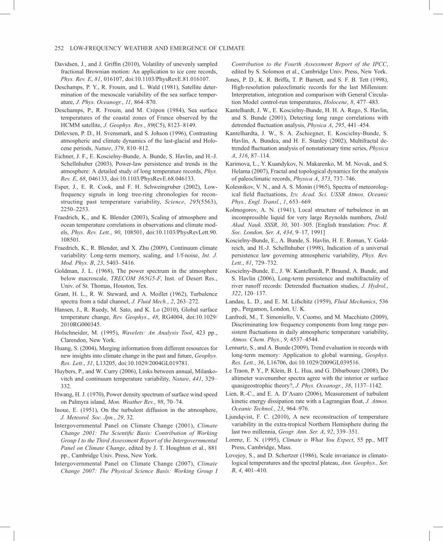
D
D
D
D
Ei
Es
Fr
Fr
G
G
H
H
H
H
H
In
In
In
Jo
K
K
K
K
K
K
K
La
La
Le
Le
Li
Lj
Lo
Lo
252 LOW-FREQUENCY WEATHER AND EMERGENCE OF CLIMATE
avidsen, J., and J. Griffin (2010), Volatility of unevenly sampledfractional Brownian motion: An application to ice core records,Phys. Rev. E, 81, 016107, doi:10.1103/PhysRevE.81.016107.eschamps, P. Y., R. Frouin, and L. Wald (1981), Satellite deter-mination of the mesoscale variability of the sea surface temper-ature, J. Phys. Oceanogr., 11, 864–870.eschamps, P., R. Frouin, and M. Crépon (1984), Sea surfacetemperatures of the coastal zones of France observed by theHCMM satellite, J. Geophys. Res., 89(C5), 8123–8149.itlevsen, P. D., H. Svensmark, and S. Johson (1996), Contrastingatmospheric and climate dynamics of the last-glacial and Holo-cene periods, Nature, 379, 810–812.chner, J. F., E. Koscielny-Bunde, A. Bunde, S. Havlin, and H.-J.Schellnhuber (2003), Power-law persistence and trends in theatmosphere: A detailed study of long temperature records, Phys.Rev. E, 68, 046133, doi:10.1103/PhysRevE.68.046133.per, J., E. R. Cook, and F. H. Schweingruber (2002), Low-frequency signals in long tree-ring chronologies for recon-structing past temperature variability, Science, 295(5563),2250–2253.aedrich, K., and K. Blender (2003), Scaling of atmosphere andocean temperature correlations in observations and climate mod-els, Phys. Rev. Lett., 90, 108501, doi:10.1103/PhysRevLett.90.108501.aedrich, K., R. Blender, and X. Zhu (2009), Continuum climatevariability: Long-term memory, scaling, and 1/f-noise, Int. J.Mod. Phys. B, 23, 5403–5416.oldman, J. L. (1968), The power spectrum in the atmospherebelow macroscale, TRECOM 365G5-F, Inst. of Desert Res.,Univ. of St. Thomas, Houston, Tex.rant, H. L., R. W. Steward, and A. Moillet (1962), Turbulencespectra from a tidal channel, J. Fluid Mech., 2, 263–272.ansen, J., R. Ruedy, M. Sato, and K. Lo (2010), Global surfacetemperature change, Rev. Geophys., 48, RG4004, doi:10.1029/2010RG000345.olschneider, M. (1995), Wavelets: An Analysis Tool, 423 pp.,Clarendon, New York.uang, S. (2004), Merging information from different resources fornew insights into climate change in the past and future, Geophys.Res. Lett., 31, L13205, doi:10.1029/2004GL019781.uybers, P., and W. Curry (2006), Links between annual, Milanko-vitch and continuum temperature variability, Nature, 441, 329–332.wang, H. J. (1970), Power density spectrum of surface wind speedon Palmyra island, Mon. Weather Rev., 98, 70–74.oue, E. (1951), On the turbulent diffusion in the atmosphere,J. Meteorol. Soc. Jpn., 29, 32.tergovernmental Panel on Climate Change (2001), ClimateChange 2001: The Scientific Basis: Contribution of WorkingGroup I to the Third Assessment Report of the IntergovernmentalPanel on Climate Change, edited by J. T. Houghton et al., 881pp., Cambridge Univ. Press, New York.tergovernmental Panel on Climate Change (2007), ClimateChange 2007: The Physical Science Basis: Working Group I
Contribution to the Fourth Assessment Report of the IPCC,edited by S. Solomon et al., Cambridge Univ. Press, New York.nes, P. D., K. R. Briffa, T. P. Barnett, and S. F. B. Tett (1998),High-resolution paleoclimatic records for the last Millenium:Interpretation, integration and comparison with General Circula-tion Model control-run temperatures, Holocene, 8, 477–483.antelhardt, J. W., E. Koscielny-Bunde, H. H. A. Rego, S. Havlin,and S. Bunde (2001), Detecting long range correlations withdetrended fluctuation analysis, Physica A, 295, 441–454.antelhardta, J. W., S. A. Zschiegner, E. Koscielny-Bunde, S.Havlin, A. Bundea, and H. E. Stanley (2002), Multifractal de-trended fluctuation analysis of nonstationary time series, PhysicaA, 316, 87–114.arimova, L., Y. Kuandykov, N. Makarenko, M. M. Novak, and S.Helama (2007), Fractal and topological dynamics for the analysisof paleoclimatic records, Physica A, 373, 737–746.olesnikov, V. N., and A. S. Monin (1965), Spectra of meteorolog-ical field fluctuations, Izv. Acad. Sci. USSR Atmos. OceanicPhys., Engl. Transl., 1, 653–669.olmogorov, A. N. (1941), Local structure of turbulence in anincompressible liquid for very large Reynolds numbers, Dokl.Akad. Nauk. SSSR, 30, 301–305. [English translation: Proc. R.Soc. London, Ser. A, 434, 9–17, 1991]oscielny-Bunde, E., A. Bunde, S. Havlin, H. E. Roman, Y. Gold-reich, and H.-J. Schellnhuber (1998), Indication of a universalpersistence law governing atmospheric variability, Phys. Rev.Lett., 81, 729–732.oscielny-Bunde, E., J. W. Kantelhardt, P. Braund, A. Bunde, andS. Havlin (2006), Long-term persistence and multifractality ofriver runoff records: Detrended fluctuation studies, J. Hydrol.,322, 120–137.ndau, L. D., and E. M. Lifschitz (1959), Fluid Mechanics, 536pp., Pergamon, London, U. K.nfredi, M., T. Simoniello, V. Cuomo, and M. Macchiato (2009),Discriminating low frequency components from long range per-sistent fluctuations in daily atmospheric temperature variability,Atmos. Chem. Phys., 9, 4537–4544.nnartz, S., and A. Bunde (2009), Trend evaluation in records withlong-term memory: Application to global warming, Geophys.Res. Lett., 36, L16706, doi:10.1029/2009GL039516.Traon, P. Y., P. Klein, B. L. Hua, and G. Dibarboure (2008), Doaltimeter wavenumber spectra agree with the interior or surfacequasigeostrophic theory?, J. Phys. Oceanogr., 38, 1137–1142.en, R.-C., and E. A. D’Asaro (2006), Measurement of turbulentkinetic energy dissipation rate with a Lagrangian float, J. Atmos.Oceanic Technol., 23, 964–976.undqvist, F. C. (2010), A new reconstruction of temperaturevariability in the extra-tropical Northern Hemisphere during thelast two millennia, Geogr. Ann. Ser. A, 92, 339–351.renz, E. N. (1995), Climate is What You Expect, 55 pp., MITPress, Cambridge, Mass.vejoy, S., and D. Schertzer (1986), Scale invariance in climato-logical temperatures and the spectral plateau, Ann. Geophys., Ser.B, 4, 401–410.
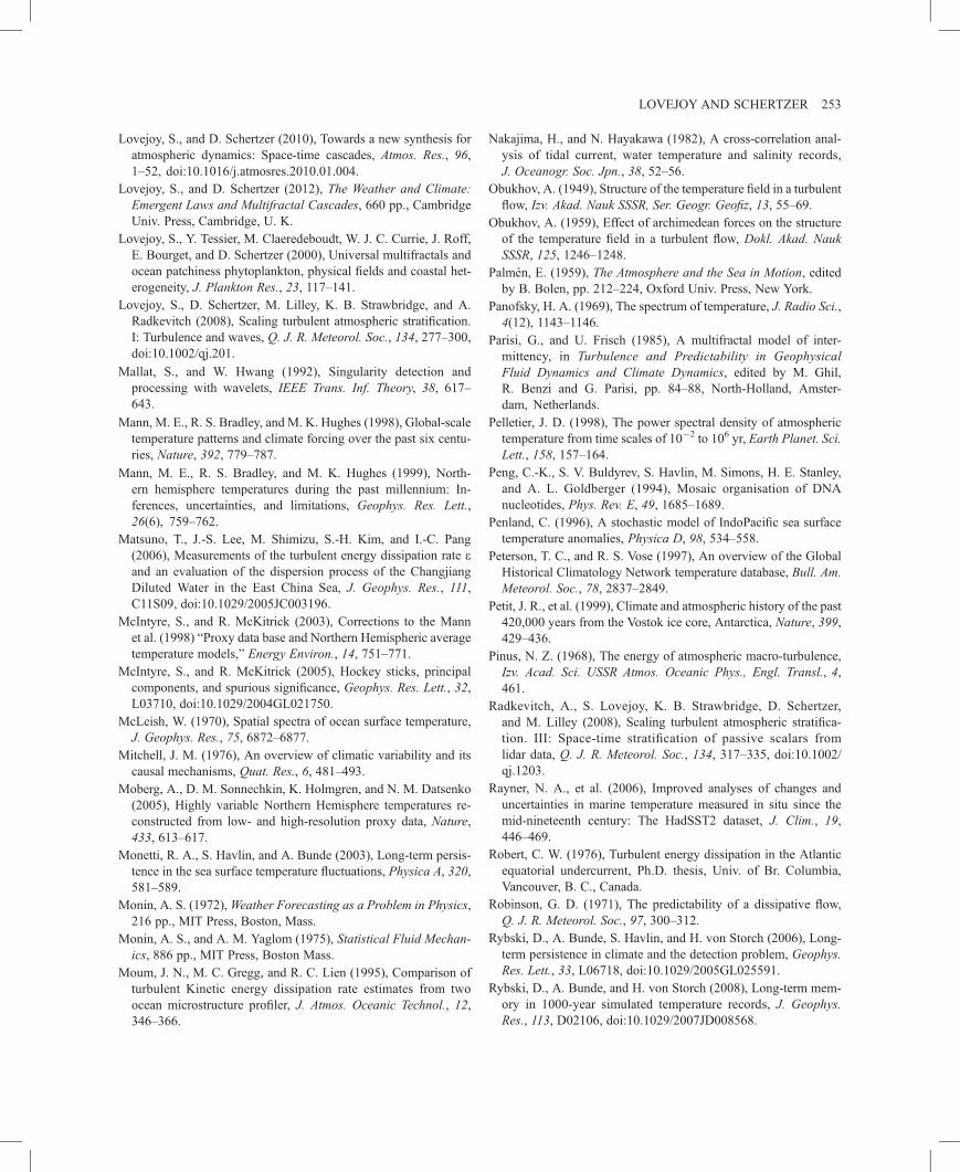
Lo
Lo
Lo
Lo
M
M
M
M
M
M
M
M
M
M
M
M
M
N
O
O
Pa
Pa
Pa
Pe
Pe
Pe
Pe
Pe
Pi
Ra
Ra
Ro
Ro
Ry
Ry
LOVEJOY AND SCHERTZER 253
vejoy, S., and D. Schertzer (2010), Towards a new synthesis foratmospheric dynamics: Space-time cascades, Atmos. Res., 96,1–52, doi:10.1016/j.atmosres.2010.01.004.vejoy, S., and D. Schertzer (2012), The Weather and Climate:Emergent Laws and Multifractal Cascades, 660 pp., CambridgeUniv. Press, Cambridge, U. K.vejoy, S., Y. Tessier, M. Claeredeboudt, W. J. C. Currie, J. Roff,E. Bourget, and D. Schertzer (2000), Universal multifractals andocean patchiness phytoplankton, physical fields and coastal het-erogeneity, J. Plankton Res., 23, 117–141.vejoy, S., D. Schertzer, M. Lilley, K. B. Strawbridge, and A.Radkevitch (2008), Scaling turbulent atmospheric stratification.I: Turbulence and waves, Q. J. R. Meteorol. Soc., 134, 277–300,doi:10.1002/qj.201.
allat, S., and W. Hwang (1992), Singularity detection andprocessing with wavelets, IEEE Trans. Inf. Theory, 38, 617–643.
ann, M. E., R. S. Bradley, and M. K. Hughes (1998), Global-scaletemperature patterns and climate forcing over the past six centu-ries, Nature, 392, 779–787.
ann, M. E., R. S. Bradley, and M. K. Hughes (1999), North-ern hemisphere temperatures during the past millennium: In-ferences, uncertainties, and limitations, Geophys. Res. Lett.,26(6), 759–762.atsuno, T., J.-S. Lee, M. Shimizu, S.-H. Kim, and I.-C. Pang(2006), Measurements of the turbulent energy dissipation rate eand an evaluation of the dispersion process of the ChangjiangDiluted Water in the East China Sea, J. Geophys. Res., 111,C11S09, doi:10.1029/2005JC003196.cIntyre, S., and R. McKitrick (2003), Corrections to the Mannet al. (1998) “Proxy data base and Northern Hemispheric averagetemperature models,” Energy Environ., 14, 751–771.cIntyre, S., and R. McKitrick (2005), Hockey sticks, principalcomponents, and spurious significance, Geophys. Res. Lett., 32,L03710, doi:10.1029/2004GL021750.cLeish, W. (1970), Spatial spectra of ocean surface temperature,J. Geophys. Res., 75, 6872–6877.itchell, J. M. (1976), An overview of climatic variability and itscausal mechanisms, Quat. Res., 6, 481–493.oberg, A., D. M. Sonnechkin, K. Holmgren, and N. M. Datsenko(2005), Highly variable Northern Hemisphere temperatures re-constructed from low- and high-resolution proxy data, Nature,433, 613–617.onetti, R. A., S. Havlin, and A. Bunde (2003), Long-term persis-tence in the sea surface temperature fluctuations, Physica A, 320,581–589.onin, A. S. (1972),Weather Forecasting as a Problem in Physics,216 pp., MIT Press, Boston, Mass.onin, A. S., and A. M. Yaglom (1975), Statistical Fluid Mechan-ics, 886 pp., MIT Press, Boston Mass.oum, J. N., M. C. Gregg, and R. C. Lien (1995), Comparison ofturbulent Kinetic energy dissipation rate estimates from twoocean microstructure profiler, J. Atmos. Oceanic Technol., 12,346–366.
akajima, H., and N. Hayakawa (1982), A cross-correlation anal-ysis of tidal current, water temperature and salinity records,J. Oceanogr. Soc. Jpn., 38, 52–56.bukhov, A. (1949), Structure of the temperature field in a turbulentflow, Izv. Akad. Nauk SSSR, Ser. Geogr. Geofiz, 13, 55–69.bukhov, A. (1959), Effect of archimedean forces on the structureof the temperature field in a turbulent flow, Dokl. Akad. NaukSSSR, 125, 1246–1248.lmén, E. (1959), The Atmosphere and the Sea in Motion, editedby B. Bolen, pp. 212–224, Oxford Univ. Press, New York.nofsky, H. A. (1969), The spectrum of temperature, J. Radio Sci.,4(12), 1143–1146.risi, G., and U. Frisch (1985), A multifractal model of inter-mittency, in Turbulence and Predictability in GeophysicalFluid Dynamics and Climate Dynamics, edited by M. Ghil,R. Benzi and G. Parisi, pp. 84–88, North-Holland, Amster-dam, Netherlands.lletier, J. D. (1998), The power spectral density of atmospherictemperature from time scales of 10�2 to 106 yr, Earth Planet. Sci.Lett., 158, 157–164.ng, C.-K., S. V. Buldyrev, S. Havlin, M. Simons, H. E. Stanley,and A. L. Goldberger (1994), Mosaic organisation of DNAnucleotides, Phys. Rev. E, 49, 1685–1689.nland, C. (1996), A stochastic model of IndoPacific sea surfacetemperature anomalies, Physica D, 98, 534–558.terson, T. C., and R. S. Vose (1997), An overview of the GlobalHistorical Climatology Network temperature database, Bull. Am.Meteorol. Soc., 78, 2837–2849.tit, J. R., et al. (1999), Climate and atmospheric history of the past420,000 years from the Vostok ice core, Antarctica, Nature, 399,429–436.nus, N. Z. (1968), The energy of atmospheric macro-turbulence,Izv. Acad. Sci. USSR Atmos. Oceanic Phys., Engl. Transl., 4,461.dkevitch, A., S. Lovejoy, K. B. Strawbridge, D. Schertzer,and M. Lilley (2008), Scaling turbulent atmospheric stratifica-tion. III: Space-time stratification of passive scalars fromlidar data, Q. J. R. Meteorol. Soc., 134, 317–335, doi:10.1002/qj.1203.yner, N. A., et al. (2006), Improved analyses of changes anduncertainties in marine temperature measured in situ since themid-nineteenth century: The HadSST2 dataset, J. Clim., 19,446–469.bert, C. W. (1976), Turbulent energy dissipation in the Atlanticequatorial undercurrent, Ph.D. thesis, Univ. of Br. Columbia,Vancouver, B. C., Canada.binson, G. D. (1971), The predictability of a dissipative flow,Q. J. R. Meteorol. Soc., 97, 300–312.bski, D., A. Bunde, S. Havlin, and H. von Storch (2006), Long-term persistence in climate and the detection problem, Geophys.Res. Lett., 33, L06718, doi:10.1029/2005GL025591.bski, D., A. Bunde, and H. von Storch (2008), Long-term mem-ory in 1000-year simulated temperature records, J. Geophys.Res., 113, D02106, doi:10.1029/2007JD008568.
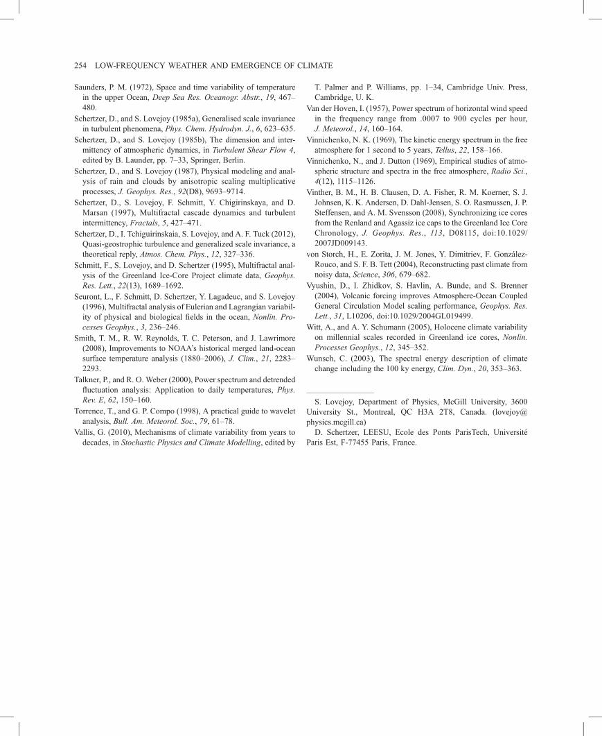
Sa
Sc
Sc
Sc
Sc
Sc
Sc
Se
Sm
Ta
To
Va
Va
Vi
Vi
Vi
vo
Vy
W
W
254 LOW-FREQUENCY WEATHER AND EMERGENCE OF CLIMATE
unders, P. M. (1972), Space and time variability of temperaturein the upper Ocean, Deep Sea Res. Oceanogr. Abstr., 19, 467–480.hertzer, D., and S. Lovejoy (1985a), Generalised scale invariancein turbulent phenomena, Phys. Chem. Hydrodyn. J., 6, 623–635.hertzer, D., and S. Lovejoy (1985b), The dimension and inter-mittency of atmospheric dynamics, in Turbulent Shear Flow 4,edited by B. Launder, pp. 7–33, Springer, Berlin.hertzer, D., and S. Lovejoy (1987), Physical modeling and anal-ysis of rain and clouds by anisotropic scaling multiplicativeprocesses, J. Geophys. Res., 92(D8), 9693–9714.hertzer, D., S. Lovejoy, F. Schmitt, Y. Chigirinskaya, and D.Marsan (1997), Multifractal cascade dynamics and turbulentintermittency, Fractals, 5, 427–471.hertzer, D., I. Tchiguirinskaia, S. Lovejoy, and A. F. Tuck (2012),Quasi-geostrophic turbulence and generalized scale invariance, atheoretical reply, Atmos. Chem. Phys., 12, 327–336.hmitt, F., S. Lovejoy, and D. Schertzer (1995), Multifractal anal-ysis of the Greenland Ice-Core Project climate data, Geophys.Res. Lett., 22(13), 1689–1692.uront, L., F. Schmitt, D. Schertzer, Y. Lagadeuc, and S. Lovejoy(1996), Multifractal analysis of Eulerian and Lagrangian variabil-ity of physical and biological fields in the ocean, Nonlin. Pro-cesses Geophys., 3, 236–246.ith, T. M., R. W. Reynolds, T. C. Peterson, and J. Lawrimore(2008), Improvements to NOAA’s historical merged land-oceansurface temperature analysis (1880–2006), J. Clim., 21, 2283–2293.lkner, P., and R. O. Weber (2000), Power spectrum and detrendedfluctuation analysis: Application to daily temperatures, Phys.Rev. E, 62, 150–160.rrence, T., and G. P. Compo (1998), A practical guide to waveletanalysis, Bull. Am. Meteorol. Soc., 79, 61–78.llis, G. (2010), Mechanisms of climate variability from years todecades, in Stochastic Physics and Climate Modelling, edited by
T. Palmer and P. Williams, pp. 1–34, Cambridge Univ. Press,Cambridge, U. K.n der Hoven, I. (1957), Power spectrum of horizontal wind speedin the frequency range from .0007 to 900 cycles per hour,J. Meteorol., 14, 160–164.nnichenko, N. K. (1969), The kinetic energy spectrum in the freeatmosphere for 1 second to 5 years, Tellus, 22, 158–166.nnichenko, N., and J. Dutton (1969), Empirical studies of atmo-spheric structure and spectra in the free atmosphere, Radio Sci.,4(12), 1115–1126.nther, B. M., H. B. Clausen, D. A. Fisher, R. M. Koerner, S. J.Johnsen, K. K. Andersen, D. Dahl-Jensen, S. O. Rasmussen, J. P.Steffensen, and A. M. Svensson (2008), Synchronizing ice coresfrom the Renland and Agassiz ice caps to the Greenland Ice CoreChronology, J. Geophys. Res., 113, D08115, doi:10.1029/2007JD009143.n Storch, H., E. Zorita, J. M. Jones, Y. Dimitriev, F. González-Rouco, and S. F. B. Tett (2004), Reconstructing past climate fromnoisy data, Science, 306, 679–682.ushin, D., I. Zhidkov, S. Havlin, A. Bunde, and S. Brenner(2004), Volcanic forcing improves Atmosphere-Ocean CoupledGeneral Circulation Model scaling performance, Geophys. Res.Lett., 31, L10206, doi:10.1029/2004GL019499.itt, A., and A. Y. Schumann (2005), Holocene climate variabilityon millennial scales recorded in Greenland ice cores, Nonlin.Processes Geophys., 12, 345–352.unsch, C. (2003), The spectral energy description of climatechange including the 100 ky energy, Clim. Dyn., 20, 353–363.
S. Lovejoy, Depar
tment of Physics, McGill University, 3600University St., Montreal, QC H3A 2T8, Canada. ([email protected])D. Schertzer, LEESU, Ecole des Ponts ParisTech, UniversitéParis Est, F-77455 Paris, France.