Embed Size (px)
Citation preview
POLITECNICO DI MILANO
DEPARTMENT OF MECHANICAL ENGINEERING
DOCTORAL PROGRAMME IN MECHANICAL ENGINEERING
Low Frequency Vibrations analysis
as a method for condition based monitoring system
for railway axles
Doctoral Dissertation of:
Paweł Rolek
Supervisor: Prof. Stefano Bruni Tutor: Prof. Stefano Beretta The Chair of the Doctoral Program: Prof. Bianca Maria Colosimo
2015 – cycle XXVII

1
2
Abstract
Safety on European railways is relatively high: it is one of the safest modes of transport
in Europe. Even so, it is essential to maintain and improve the current level of safety for
the benefit of its users. A safe railway is more efficient and also a more attractive transport
choice, which meets the needs of society due to increasing mobility.
Railway vehicle is composed of many different elements, from which some are critical
from safety point of view. One of such kind of elements are the axles, thus special attention
to their health needs to be paid. They are mechanical components working under effects
of rotating bending at high number of cycles. To prevent failure of the axles working under
this demanding conditions, periodical inspections needs to be performed. Railway axles
in modern vehicles are not only transferring load but also providing support for brakes and
other auxiliary systems, thus their proper inspection against faults often requires complete
disassembling process and use of one of the non-destructive diagnostic techniques. This
approach has significant disadvantages: inspection needs to be performed in workshop
which is time, effort and money consuming. Due to the lack of information about the state
of the axle during its operation the inspections are scheduled periodically on time or
kilometre basis, which can cause either money loss for operator in case of unnecessary
check (no problems found) or serious accident in case of axle failure due to overcome its
critical condition before planned inspection.
In this work analysis of possible application of ale bending vibration measurement as
a method for monitoring the structural integrity of railway axles is presented.
After an examination of the State of The Art, results of full scale tests performed on
cracked axles are presented, showing the feasibility of this monitoring approach.
Next, a Finite Element model of the rotating cracked axle is developed and used to
investigate the size of recognisable defects together with the effect of various sources of
disturbance, namely track irregularity and wheel out-of-roundness.
The final results of the research showed that the increasing vibration signal
components (mainly 1xRev and 2xRev) are promising indicators of axle fault development
and they can be fruitfully measured and monitored by proposed system.
The increase of vibration components amplitudes was reaching up to ten times the
values recorded when no crack was existing in the axle. The level of vibration components
and knowledge about possible crack growth rate in railway axle allows to assume that LFV
method can provide diagnostic information during service of railway vehicle, also when
wheels are undergoing degradation process, thus developing greater out of roundness
profiles which are introducing additional excitation in measured system.
3
Contents
0. Introduction .................................................................................................................. 7
1. Non-destructive Fault Detection Techniques for railway wheelsets ....................... 10
1.1. Railway axles: role, requirements ................................................................ 10
1.2. Fatigue assessment of railway axles ........................................................... 11
1.3. Railway axles failures ................................................................................... 12
1.4. Defect detection methods in condition based monitoring of railway
wheelsets ....................................................................................................... 16
2. Crack-related vibrations in rotating shafts ................................................................ 23
2.1. Cracks in rotating shafts............................................................................... 24
2.1.1. Crack propagation in rotating shafts .................................................. 24
2.1.2. Crack breathing mechanism ............................................................. 26
2.1.3. Dynamic behavior of cracked shafts ................................................. 28
2.2. Crack modelling ............................................................................................ 30
2.2.1. Types of crack models used in simulations ....................................... 30
2.2.2. Influence of the crack shape on simulation results ............................ 34
3. Laboratory tests .......................................................................................................... 36
3.1. Laboratory test of cracked axles .................................................................. 36
3.2. Experiment set-up ......................................................................................... 36
3.3. Experiment procedure .................................................................................. 38
3.4. Data acquisition ............................................................................................. 39
3.4.1. Sensors in laboratory test ................................................................. 39
3.4.2. Signal processing ............................................................................. 41
3.4.2.1. Anti-aliasing ...................................................................................... 42
3.4.2.2. Signal synchronization (triggering) ................................................... 43
3.4.2.3. Synchronous averaging .................................................................... 43
3.4.2.4. Order analysis and windowing .......................................................... 44
3.4.2.5. Initial vibration level extraction .......................................................... 45
3.4.2.6. Fast Fourier Transform (FFT) ........................................................... 45
3.4.3. Signal processing summary .............................................................. 46
4
3.5. Experiment results ........................................................................................ 47
3.6. Experiment conclusions ............................................................................... 51
4. Finite Element Model .................................................................................................. 52
4.1. 3D Finite Element Method model ................................................................. 52
4.2. Geometrical model of railway axle ............................................................... 52
4.3. Finite element model of cracked railway axle ............................................. 53
4.3.1. Model definition ................................................................................ 55
4.3.2. Cracked area modelling .................................................................... 56
4.3.3. Boundary conditions ......................................................................... 60
4.3.4. Load definition .................................................................................. 61
4.3.5. Damping in model ............................................................................. 62
4.4. Simulation scenarios .................................................................................... 64
4.4.1. Laboratory case setup ...................................................................... 64
4.4.2. ‘Railway’ case setup ......................................................................... 64
4.4.2.1. No excitation in model ...................................................................... 65
4.4.2.2. Wheel out of roundness excitations .................................................. 65
4.4.2.3. Wheel-rail interaction excitations ...................................................... 69
4.5. Simulation results ......................................................................................... 71
4.5.1. Laboratory case simulation results .................................................... 71
4.5.2. Railway case simulation results ........................................................ 76
CONCLUSIONS ................................................................................................................ 89
ACKNOWLEDGEMENTS ................................................................................................. 92
BIBLIOGRAPHY ............................................................................................................... 93
5
List of figures:
Figure 0.1 Significant accidents per type of accidents (EU-28:2010-2012)[1] ......................................... 7 Figure 0.2 Breakdown of number of derailments in Europe into major causes categories [2] .................. 8 Figure 1.1 Types of railway axles ........................................................................................................... 11 Figure 1.2 Different kind of damaging of an in-service railway axle ........................................................ 13 Figure 1.3 Crack growth rate due to impact [15] ..................................................................................... 14 Figure 1.4 Crack growth models due to combined action of corrosion fatigue........................................ 14 Figure 1.5 Example of POD curve for hollow axle inspection (10% threshold) [23] ................................ 15 Figure 1.6 Simple definition of the inspection interval, from the crack growth simulation [11] ................ 15 Figure 1.7 Railway axle failure [3] ........................................................................................................... 16 Figure 1.8 Schematic representation of Phased Array Probe ................................................................. 18 Figure 1.9 Phased array working principle ............................................................................................. 19 Figure 1.10 Principle of the conical phased array probe ......................................................................... 19 Figure 1.11 AC thermography method [33]............................................................................................. 20 Figure 1.12 AE theory principle .............................................................................................................. 21 Figure 1.13 AE application in railway axle crack detection tests............................................................ 21 Figure 1.14 High Frequency Response of cracked axles ....................................................................... 22 Figure 2.1 Cracked axle cross section with visible crack rest lines ......................................................... 25 Figure 2.2 Vibration signal amplitudes of shaft with propagating crack [51] ........................................... 26 Figure 2.3 Area in contact between crack surfaces as a function of axle rotation .................................. 27 Figure 2.4 First and Second harmonic component of cracked shaft vibration signal [66] ....................... 29 Figure 2.5 Vertical displacement as function of cracked beam angular position [68] .............................. 32 Figure 2.6 Vertical displacement of cracked shaft, comparison between measured
and calculated deflections [68] ............................................................................................. 33 Figure 2.7 Lateral deflection of 30% cracked shaft with different shear loads applied [68] ..................... 33 Figure 2.8 Vertical vibration components dependence on crack depth [68]............................................ 34 Figure 2.9 Vibration signal harmonic components in case of rectilinear crack shape [68] ...................... 35 Figure 2.10 Vibration signal harmonic components in case of elliptical crack shape [68] ....................... 35 Figure 3.1 Dynamic Test Bench for Railway Axles ............................................................................... 37 Figure 3.2 Drawing of full-scale specimen example ............................................................................... 37 Figure 3.3 Scheme of the full-scale axle equipped with transducers ...................................................... 38 Figure 3.4 Laser sensor head and main control unit .............................................................................. 40 Figure 3.5 Data acquisition system: ....................................................................................................... 41 Figure 3.6 Input signal not periodic in time record .................................................................................. 43 Figure 3.7 Input signal periodic in time record ........................................................................................ 43 Figure 3.8 Axle speed determination using once per revolution tachometer pulse ................................. 42 Figure 3.9 Synchronous averaging ......................................................................................................... 44 Figure 3.10 Signal processing scheme ................................................................................................... 46 Figure 3.11 Polar plot of vibration from one revolution of axle and its corresponding spectra ................ 47 Figure 3.12 Comparison of harmonics trends of vibration signals from axles tests ................................ 49 Figure 3.13 1xRev (first order) harmonic comparison ............................................................................ 50 Figure 3.14 2xRev (second order) harmonic comparison ...................................................................... 50 Figure 3.15 Harmonics of vibration signal from axle with no fault development during test .................... 51 Figure 4.1 Geometrical model of railway axle ......................................................................................... 53 Figure 4.2 Full and reduced integration method in 8-nodes element [93] ............................................... 53 Figure 4.3 Hourglass effect in reduced integration element type due to applied moment [94] ............... 54 Figure 4.4 Hourglass control energy verification ..................................................................................... 55 Figure 4.5 Finite Element model of railway axle ..................................................................................... 55 Figure 4.6 Partitioning of cracked axle model ......................................................................................... 56 Figure 4.7 Reduced possibility of master-slave surface penetration in S-to-S contact type [98] ............ 57 Figure 4.8 'Hard contact' formulation for pressure-overclosure behaviour [98] ....................................... 58 Figure 4.9 Friction model in contact area [99]......................................................................................... 59 Figure 4.10 Specimen in crack opening situation (100x magnified in crack opening direction) .............. 59 Figure 4.11 Closed crack and resulting contact pressure area ............................................................... 60 Figure 4.12 Additional axle deflection due to influence of crack breathing mechanism .......................... 60 Figure 4.13 Boundary conditions defined in model ................................................................................. 61 Figure 4.14 Load definition in model ....................................................................................................... 62 Figure 4.15 Rayleigh damping coefficients and resulting damping ratio ................................................. 63
6
Figure 4.16 Influence of damping on axle vibration decay ...................................................................... 63 Figure 4.17 'Laboratory case' model definition scheme .......................................................................... 64 Figure 4.18 'Railway' case model definition scheme ............................................................................... 65 Figure 4.19 New wheel OOR profile versus wheel circumferential coordinate........................................ 67 Figure 4.20 Extended wheel OOR profile and its corresponding spectra ............................................... 67 Figure 4.21 Worn wheel out of roundness profile ................................................................................... 68 Figure 4.22 Extended worn wheel OOR profile (upper) and its corresponding spectra (lower) .............. 68 Figure 4.23 Rail irregularity profile .......................................................................................................... 69 Figure 4.24 Common excitation for wheel and rail used in simulation .................................................... 70 Figure 4.25 Non-cracked axle deflections and its corresponding harmonic components ....................... 71 Figure 4.26 Deflection and spectra components for defined crack depth ............................................... 72 Figure 4.27 Harmonic components amplitude trend as function of crack depth ..................................... 75 Figure 4.28 Vertical displacement components (FFT) for 35% crack, no external source
of excitation in model ........................................................................................................... 76 Figure 4.29 Harmonic components (FFT) of axle vertical vibrations influenced by 'new' OOR profiles .. 77 Figure 4.30 Comparison of harmonic components amplitudes (‘new’ wheel OOR) ................................ 78 Figure 4.31 Harmonic components (FFT) of axle vertical vibrations influenced by 'worn' OOR profiles . 79 Figure 4.32 Comparison of harmonic components amplitudes (‘worn’ wheel OOR profile) .................... 80 Figure 4.33 Axle vertical vibration from 'Mixed case' simulation results (under ‘new’ wheel OOR
and rail profile influence)...................................................................................................... 81 Figure 4.34 Axle vertical vibration from ‘Mixed case' simulation results (under ‘new’ OOR profile,
rail profile and 35% crack depth influence ........................................................................... 82 Figure 4.35 Comparison of harmonic components amplitudes (‘new’ wheel OOR and rail
irregularities included) ......................................................................................................... 83 Figure 4.36 Axle vertical vibration from 'Mixed case' simulation results (under ‘worn’ OOR profile
and rail profile influence)...................................................................................................... 84 Figure 4.37 Axle vertical vibration from 'Mixed case' simulation results (under ‘worn’ OOR profile,
rail profile and 35% crack depth influence) .......................................................................... 85 Figure 4.38 Comparison of harmonic components amplitudes (‘worn’ wheel OOR and rail
irregularities included) ......................................................................................................... 86 Figure 4.39 FFT of axle vertical vibration from 'Mixed case' simulation results including ‘worn’
OOR profile, rail irregularity profile and 30% deep crack influence ...................................... 87 Figure 4.40 Change in NxRev components due to crack size (excitations from ‘worn’ wheel OOR
and rail irregularities included) ............................................................................................. 87
7
0. Introduction
Safety on European railways is relatively high allowing to formulate the statement that
it is one of the safest modes of transport in Europe [1].
Even so, it is essential to maintain and even improve the current level of safety for the
benefit of its users and to meet the European rail network strategy of targeting
considerable expansion of passenger and freight traffic by year 2020.
According to the common safety indicators data, railway safety continued to improve
across the EU, but despite a general improvement, there has been no progress in reducing
the number of several types of accidents, from witch 5% of total accidents is tied up to
train collisions and derailments [1]. As European Railway Agency reports, the number of
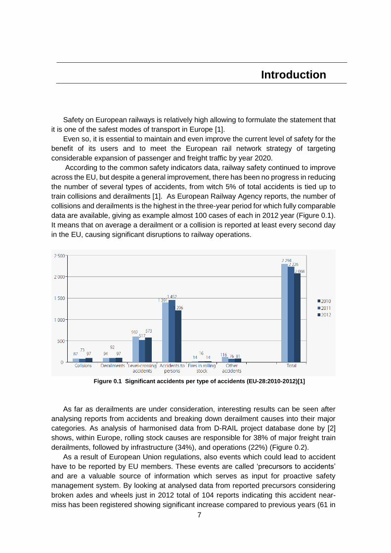
collisions and derailments is the highest in the three-year period for which fully comparable
data are available, giving as example almost 100 cases of each in 2012 year (Figure 0.1).
It means that on average a derailment or a collision is reported at least every second day
in the EU, causing significant disruptions to railway operations.
Figure 0.1 Significant accidents per type of accidents (EU-28:2010-2012)[1]
As far as derailments are under consideration, interesting results can be seen after
analysing reports from accidents and breaking down derailment causes into their major
categories. As analysis of harmonised data from D-RAIL project database done by [2]
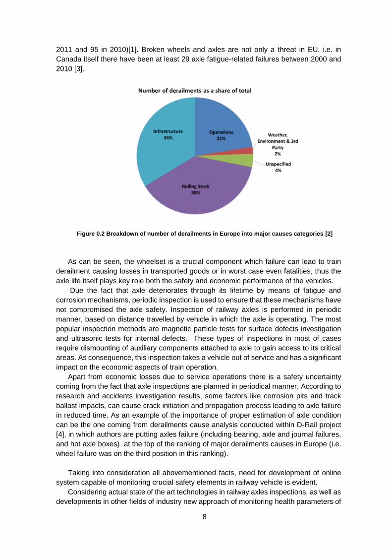
shows, within Europe, rolling stock causes are responsible for 38% of major freight train
derailments, followed by infrastructure (34%), and operations (22%) (Figure 0.2).
As a result of European Union regulations, also events which could lead to accident
have to be reported by EU members. These events are called ‘precursors to accidents’
and are a valuable source of information which serves as input for proactive safety
management system. By looking at analysed data from reported precursors considering
broken axles and wheels just in 2012 total of 104 reports indicating this accident near-
miss has been registered showing significant increase compared to previous years (61 in
8
2011 and 95 in 2010)[1]. Broken wheels and axles are not only a threat in EU, i.e. in
Canada itself there have been at least 29 axle fatigue-related failures between 2000 and
2010 [3].
Figure 0.2 Breakdown of number of derailments in Europe into major causes categories [2]
As can be seen, the wheelset is a crucial component which failure can lead to train
derailment causing losses in transported goods or in worst case even fatalities, thus the
axle life itself plays key role both the safety and economic performance of the vehicles.
Due the fact that axle deteriorates through its lifetime by means of fatigue and
corrosion mechanisms, periodic inspection is used to ensure that these mechanisms have
not compromised the axle safety. Inspection of railway axles is performed in periodic
manner, based on distance travelled by vehicle in which the axle is operating. The most
popular inspection methods are magnetic particle tests for surface defects investigation
and ultrasonic tests for internal defects. These types of inspections in most of cases
require dismounting of auxiliary components attached to axle to gain access to its critical
areas. As consequence, this inspection takes a vehicle out of service and has a significant
impact on the economic aspects of train operation.
Apart from economic losses due to service operations there is a safety uncertainty
coming from the fact that axle inspections are planned in periodical manner. According to
research and accidents investigation results, some factors like corrosion pits and track
ballast impacts, can cause crack initiation and propagation process leading to axle failure
in reduced time. As an example of the importance of proper estimation of axle condition
can be the one coming from derailments cause analysis conducted within D-Rail project
[4], in which authors are putting axles failure (including bearing, axle and journal failures,
and hot axle boxes) at the top of the ranking of major derailments causes in Europe (i.e.
wheel failure was on the third position in this ranking).
Taking into consideration all abovementioned facts, need for development of online
system capable of monitoring crucial safety elements in railway vehicle is evident.
Considering actual state of the art technologies in railway axles inspections, as well as
developments in other fields of industry new approach of monitoring health parameters of
9
railway axle during its operation is proposed. The methodology for estimating the condition
of axle is based on so called breathing mechanism of eventual crack, which is affecting
the bending stiffness and thus generating additional vibration due to rotation of the axle
during operation. Specific patterns of this vibration, namely NxRev components (harmonic
components at frequencies that are integer multiples of the frequency of rotation) can be
used for the fault detection purposes, leading to the continuous structural health
monitoring of the axle.
More detailed theoretical considerations, as well as feasibility study for applying LFV
methodology in railway axle monitoring system will be closer described in following
chapters of this work:
Chapter 1: In this chapter role of railway wheelsets and basic concepts of design
requirements are briefly introduced. Next, railway wheelsets monitoring systems are listed
and briefly described to give a reader insight of currently leading edge technology of non-
destructive testing.
Chapter 2: Here vibrations of rotating shafts are introduced, focusing on crack
occurrence and its influence on specific vibration spectra components. The so called crack
breathing mechanism is explained and different attempts to model it numerically to gain
proper diagnostic information about shaft health are presented.
Chapter 3: This chapter covers detailed description of preparation and conducting
laboratory tests of different types of cracked and non-cracked railway axles for
assessment of low frequency vibration analysis technique for fault detection system in
railway axles. Laboratory test results are also presented and discussion on their relevance
is included.
Chapter 4: In this chapter detailed description of Finite element Model of cracked
railway axle is included, different simulation scenarios are explained and simulation results
are presented.
Concluding discussion and comparison between experimental results and simulation
results are presented in Conclusions section at the end of work.
10
CHAPTER 1
1. Non-destructive Fault Detection Techniques
for railway wheelsets
1.1. Railway axles: role, requirements
Railway axle is mechanical component which in combination with wheels is creating
substructure named wheelset. Wheelset is providing guidance for railway vehicle, but also
needs to sustain loads coming from engines torque (in case of powered axle), braking
forces, train-track interaction and vehicle weight. All abovementioned load spectra are
causing cyclic loading of railway axle which can lead to its failure due to fatigue.
Railway axles, as they are integral part of railway wheelset, are safety critical
components. Their failure may result in derailments, causing serious damage for the rolling
stock and the infrastructure, injuries of passengers and in the most serious cases can
even lead to fatalities. Therefore, axle resistance to failure is a key issue in designing and
correctly maintaining railway vehicles, to ensure high safety standards and, at the same
time, to optimize life-cycle costs from a system point of view.
Even if high safety level is provided by the present practices of railway operation, a
continuous improvement of the safety is always recommended. Due to this fact the design
of axles was since decades approved and always adjusted according the newest State of
the Art.
Modern axles are produced mostly from two types of material, namely A1N low
strength steel grade (normalized C40 carbon steel) and medium strength A4T steel grade
(quenched 25CrMo4 alloy), with strictly described parameters [5] . Nevertheless, due to
increased demand of weight reduction and improved durability new materials for axle
production are developed and introduced in operation (ex. 30NiCrMoV12 alloyed steel
used in some Italian high speed train axles production [6]).
Two main different types of axles can be found on modern trains, axles with bore,
named hollow axles and axles with continuous cross section, named solid axles (Figure
1.1) Railway axles are designed, manufactured and maintained so that they should not
fail in service, usually targeting up to 40 years of service, or 107 km.
11
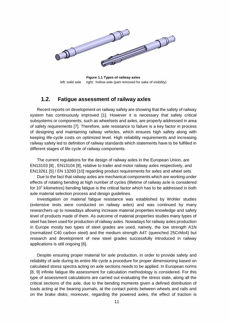
Figure 1.1 Types of railway axles
left: solid axle right: hollow axle (part removed for sake of visibility)
1.2. Fatigue assessment of railway axles
Recent reports on development on railway safety are showing that the safety of railway
system has continuously improved [1]. However it is necessary that safety critical
subsystems or components, such as wheelsets and axles, are properly addressed in area
of safety requirements [7]. Therefore, axle resistance to failure is a key factor in process
of designing and maintaining railway vehicles, which ensures high safety along with
keeping life-cycle costs on optimized level. High reliability requirements and increasing
railway safety led to definition of railway standards which statements have to be fulfilled in
different stages of life cycle of railway components.
The current regulations for the design of railway axles in the European Union, are
EN13103 [8] , EN13104 [9], relative to trailer and motor railway axles respectively, and
EN13261 [5] / EN 13260 [10] regarding product requirements for axles and wheel sets.
Due to the fact that railway axles are mechanical components which are working under
effects of rotating bending at high number of cycles (lifetime of railway axle is considered
for 107 kilometres) bending fatigue is the critical factor which has to be addressed in both
axle material selection process and design guidelines.
Investigation on material fatigue resistance was established by Wohler studies
(extensive tests were conducted on railway axles) and was continued by many
researchers up to nowadays allowing increase material properties knowledge and safety
level of products made of them. As outcome of material properties studies many types of
steel has been used for production of railway axles. Nowadays for railway axles production
in Europe mostly two types of steel grades are used, namely, the low strength A1N
(normalized C40 carbon steel) and the medium strength A4T (quenched 25CrMo4) but
research and development of new steel grades successfully introduced in railway
applications is still ongoing [6].
Despite ensuring proper material for axle production, in order to provide safety and
reliability of axle during its entire life cycle a procedure for proper dimensioning based on
calculated stress spectra acting on axle sections needs to be applied. In European norms
[8, 9] infinite fatigue life assessment for calculation methodology is considered. For this
type of assessment calculations are carried out evaluating the stress state, along all the
critical sections of the axle, due to the bending moments given a defined distribution of
loads acting at the bearing journals, at the contact points between wheels and rails and
on the brake disks; moreover, regarding the powered axles, the effect of traction is
12
considered. Due to fact that the service loads acting on a wheelset are not well known, [8,
9] adopts a combination of loads onto the axle, chosen as representative of the most
critical loading condition. The design is then performed by a simple comparison of the
stress state acting on the critical sections of the axle against the Fatigue Limit of the
involved material reduced by a generous safety factor in order to take into account all the
uncertainties about the working conditions of the wheelset during its life [11].
Another approach for the railway axle design, according to the FKM guidelines [12], is
the fatigue assessment adopting damage sum criteria derived from the concepts of
damage accumulation originally due to Miner [13]. In particular, two approaches are
proposed by the guidelines: the simplest is the Haibach model [14], identical to the original
Miner’s rule except that two regions of the fatigue curve are defined, the ‘finite life’ region
and the ‘infinite life’ one. The more complex approach, on the other hand, is represented
by the consequent Miner’s rule: when the component starts its service under variable
amplitude loadings, and in the case the load spectrum contains some cycles above the
(initial) endurance limit, these cycles will reduce it for a certain amount, and this process
of reduction progressively increase while the damage rises; as a consequence of the
phenomenon, continuing the variable amplitude loading, also the cycles of the spectrum
initially under the endurance limit begin to contribute to the damage, till the damage sum
reaches a critical value and the endurance limit gets to zero.
1.3. Railway axles failures
Railway axles, even though designed for infinite life, and severely checked before their
re-admission to operation are subject to failure due to various types of surface damage
(i.e. ballast hits, corrosion pits) that may occur during their very long service life, thus
occasional incidents have been observed in service. Due to this fact regular axle
examinations in the form of non-destructive testing inspections are performed. Period of
operation between tests is calculated on the basis of the propagation lifetime of a given
initial defect. The key point is therefore a reliable estimation of propagation lifetime under
service loads. Reported failures were caused by fatigue fracture which typically occurs at
the press-fits for wheels, gears and brakes or at the axle body mid-span and close to
transitions. Although this type of failure always occurs due to fatigue crack propagation,
its actual initiation, during the long lasting service life of axles (up to 30 years or 107 km),
can be due to various factors such as paint detachment, pitting from corrosion, damage
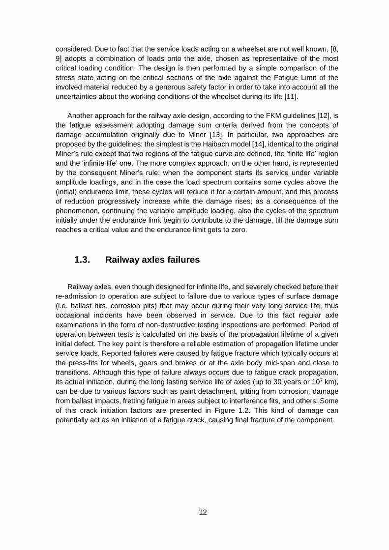
from ballast impacts, fretting fatigue in areas subject to interference fits, and others. Some
of this crack initiation factors are presented in Figure 1.2. This kind of damage can
potentially act as an initiation of a fatigue crack, causing final fracture of the component.
13
Figure 1.2 Different kind of damaging of an in-service railway axle
upper: paint detachment middle: corrosion pits lower: damage from ballast impact
credit: Lucchini RS, Italy
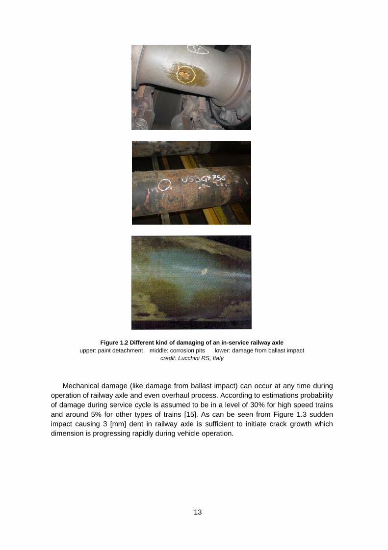
Mechanical damage (like damage from ballast impact) can occur at any time during
operation of railway axle and even overhaul process. According to estimations probability
of damage during service cycle is assumed to be in a level of 30% for high speed trains
and around 5% for other types of trains [15]. As can be seen from Figure 1.3 sudden
impact causing 3 [mm] dent in railway axle is sufficient to initiate crack growth which
dimension is progressing rapidly during vehicle operation.
14
Figure 1.3 Crack growth rate due to impact [15]
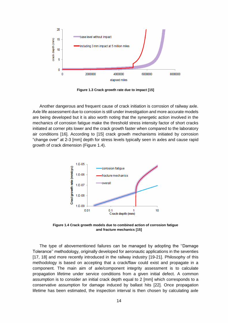
Another dangerous and frequent cause of crack initiation is corrosion of railway axle.
Axle life assessment due to corrosion is still under investigation and more accurate models
are being developed but it is also worth noting that the synergetic action involved in the
mechanics of corrosion fatigue make the threshold stress intensity factor of short cracks
initiated at corner pits lower and the crack growth faster when compared to the laboratory
air conditions [16]. According to [15] crack growth mechanisms initiated by corrosion
“change over” at 2-3 [mm] depth for stress levels typically seen in axles and cause rapid
growth of crack dimension (Figure 1.4).
Figure 1.4 Crack growth models due to combined action of corrosion fatigue
and fracture mechanics [15]
The type of abovementioned failures can be managed by adopting the ‘‘Damage
Tolerance’’ methodology, originally developed for aeronautic applications in the seventies
[17, 18] and more recently introduced in the railway industry [19-21]. Philosophy of this
methodology is based on accepting that a crack/flaw could exist and propagate in a
component. The main aim of axle/component integrity assessment is to calculate
propagation lifetime under service conditions from a given initial defect. A common
assumption is to consider an initial crack depth equal to 2 [mm] which corresponds to a
conservative assumption for damage induced by ballast hits [22]. Once propagation
lifetime has been estimated, the inspection interval is then chosen by calculating axle
15
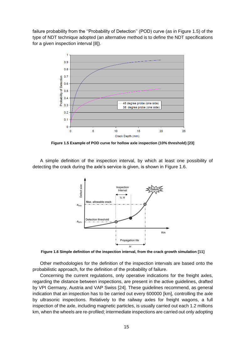
failure probability from the ‘‘Probability of Detection’’ (POD) curve (as in Figure 1.5) of the
type of NDT technique adopted (an alternative method is to define the NDT specifications
for a given inspection interval [8]).
Figure 1.5 Example of POD curve for hollow axle inspection (10% threshold) [23]
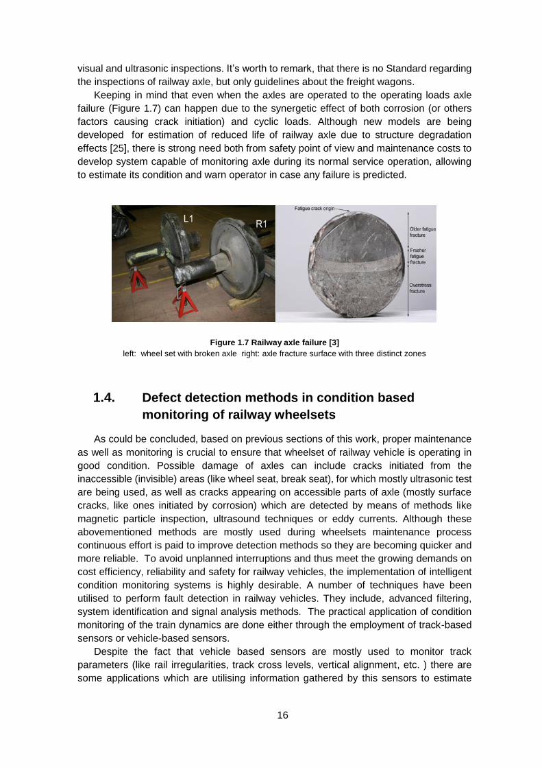
A simple definition of the inspection interval, by which at least one possibility of
detecting the crack during the axle’s service is given, is shown in Figure 1.6.
Figure 1.6 Simple definition of the inspection interval, from the crack growth simulation [11]
Other methodologies for the definition of the inspection intervals are based onto the
probabilistic approach, for the definition of the probability of failure.
Concerning the current regulations, only operative indications for the freight axles,
regarding the distance between inspections, are present in the active guidelines, drafted
by VPI Germany, Austria and VAP Swiss [24]. These guidelines recommend, as general
indication that an inspection has to be carried out every 600000 [km], controlling the axle
by ultrasonic inspections. Relatively to the railway axles for freight wagons, a full
inspection of the axle, including magnetic particles, is usually carried out each 1.2 millions
km, when the wheels are re-profiled; intermediate inspections are carried out only adopting
16
visual and ultrasonic inspections. It’s worth to remark, that there is no Standard regarding
the inspections of railway axle, but only guidelines about the freight wagons.
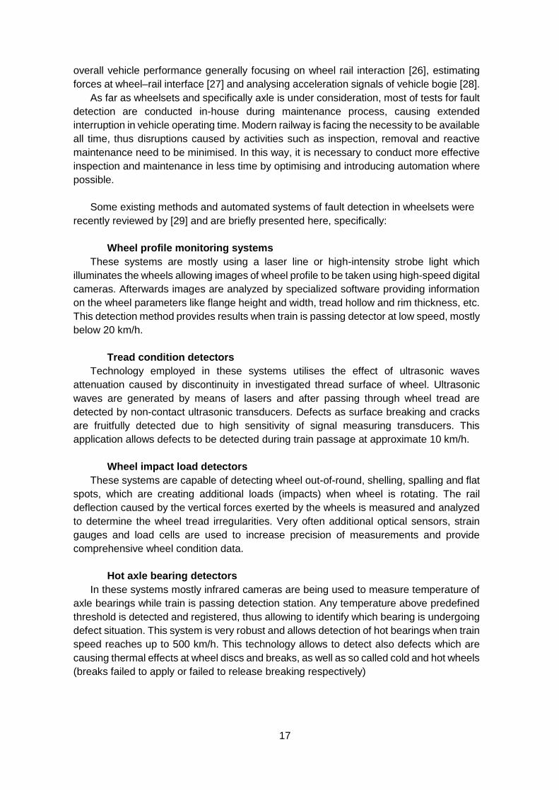
Keeping in mind that even when the axles are operated to the operating loads axle
failure (Figure 1.7) can happen due to the synergetic effect of both corrosion (or others
factors causing crack initiation) and cyclic loads. Although new models are being
developed for estimation of reduced life of railway axle due to structure degradation
effects [25], there is strong need both from safety point of view and maintenance costs to
develop system capable of monitoring axle during its normal service operation, allowing
to estimate its condition and warn operator in case any failure is predicted.
Figure 1.7 Railway axle failure [3]
left: wheel set with broken axle right: axle fracture surface with three distinct zones
1.4. Defect detection methods in condition based
monitoring of railway wheelsets
As could be concluded, based on previous sections of this work, proper maintenance
as well as monitoring is crucial to ensure that wheelset of railway vehicle is operating in
good condition. Possible damage of axles can include cracks initiated from the
inaccessible (invisible) areas (like wheel seat, break seat), for which mostly ultrasonic test
are being used, as well as cracks appearing on accessible parts of axle (mostly surface
cracks, like ones initiated by corrosion) which are detected by means of methods like
magnetic particle inspection, ultrasound techniques or eddy currents. Although these
abovementioned methods are mostly used during wheelsets maintenance process
continuous effort is paid to improve detection methods so they are becoming quicker and
more reliable. To avoid unplanned interruptions and thus meet the growing demands on
cost efficiency, reliability and safety for railway vehicles, the implementation of intelligent
condition monitoring systems is highly desirable. A number of techniques have been
utilised to perform fault detection in railway vehicles. They include, advanced filtering,
system identification and signal analysis methods. The practical application of condition
monitoring of the train dynamics are done either through the employment of track-based
sensors or vehicle-based sensors.
Despite the fact that vehicle based sensors are mostly used to monitor track
parameters (like rail irregularities, track cross levels, vertical alignment, etc. ) there are
some applications which are utilising information gathered by this sensors to estimate
17
overall vehicle performance generally focusing on wheel rail interaction [26], estimating
forces at wheel–rail interface [27] and analysing acceleration signals of vehicle bogie [28].
As far as wheelsets and specifically axle is under consideration, most of tests for fault
detection are conducted in-house during maintenance process, causing extended
interruption in vehicle operating time. Modern railway is facing the necessity to be available
all time, thus disruptions caused by activities such as inspection, removal and reactive
maintenance need to be minimised. In this way, it is necessary to conduct more effective
inspection and maintenance in less time by optimising and introducing automation where
possible.
Some existing methods and automated systems of fault detection in wheelsets were
recently reviewed by [29] and are briefly presented here, specifically:
Wheel profile monitoring systems
These systems are mostly using a laser line or high-intensity strobe light which
illuminates the wheels allowing images of wheel profile to be taken using high-speed digital
cameras. Afterwards images are analyzed by specialized software providing information
on the wheel parameters like flange height and width, tread hollow and rim thickness, etc.
This detection method provides results when train is passing detector at low speed, mostly
below 20 km/h.
Tread condition detectors
Technology employed in these systems utilises the effect of ultrasonic waves
attenuation caused by discontinuity in investigated thread surface of wheel. Ultrasonic
waves are generated by means of lasers and after passing through wheel tread are
detected by non-contact ultrasonic transducers. Defects as surface breaking and cracks
are fruitfully detected due to high sensitivity of signal measuring transducers. This
application allows defects to be detected during train passage at approximate 10 km/h.
Wheel impact load detectors
These systems are capable of detecting wheel out-of-round, shelling, spalling and flat
spots, which are creating additional loads (impacts) when wheel is rotating. The rail
deflection caused by the vertical forces exerted by the wheels is measured and analyzed
to determine the wheel tread irregularities. Very often additional optical sensors, strain
gauges and load cells are used to increase precision of measurements and provide
comprehensive wheel condition data.
Hot axle bearing detectors
In these systems mostly infrared cameras are being used to measure temperature of
axle bearings while train is passing detection station. Any temperature above predefined
threshold is detected and registered, thus allowing to identify which bearing is undergoing
defect situation. This system is very robust and allows detection of hot bearings when train
speed reaches up to 500 km/h. This technology allows to detect also defects which are
causing thermal effects at wheel discs and breaks, as well as so called cold and hot wheels
(breaks failed to apply or failed to release breaking respectively)
18
Acoustic bearing defect detectors
For defect detection in bearing array of microphones located close to the track is used.
If noise generated by passing bearing is recorded and its level is beyond defined threshold
corresponding bearing is investigated for possible faults. This system is capable of
detecting defects before they cause complete failure of bearing.
Brake pad inspection systems
Inspection method in these systems is based on image processing techniques, which
are analyzing digital picture of brake pad taken when train is passing diagnostic station,
thus providing information about brake pad wear, uneven wear and in worst case missing
pad.
Although many automated systems exists providing detection of possible faults in
wheelsets, for axle fault detection specifically, still mostly stationary methods are used,
mostly requiring to remove whole axle or some of its auxiliary components from vehicle
prior conducting test. Most popular NDT techniques are eddy current testing, magnetic
particles and ultrasonic tests. In general surface NDT methods (i.e. magnetic particle
inspection, eddy currents) can be used when the axle body is inspected except areas
where access is restricted for example where there is no visual and/or hand access. For
cracks under the wheel seat (for example) surface inspection methods can be used only
when the wheels are removed. Internal defects as well as those located at inaccessible
areas are mostly investigated by means of ultrasonic tests. Nevertheless of stationary
nature of abovementioned tests improvements are introduced to shorten the testing time
and thus reduce interruption in vehicle service, as well as new methods are introduced to
allow inspection on moving train. Few chosen methods already in use in stationary testing
as well as most promising methods for axle tests on moving train are briefly introduced
here.
Phased array detection
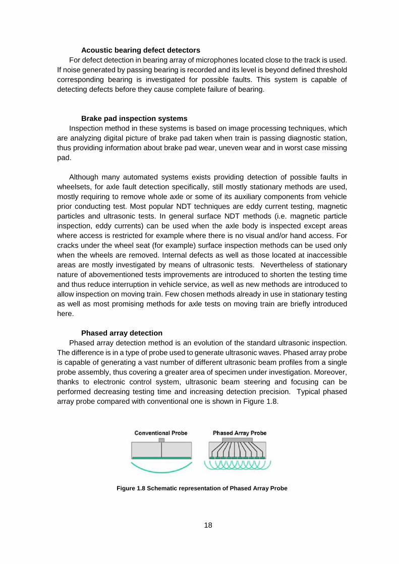
Phased array detection method is an evolution of the standard ultrasonic inspection.
The difference is in a type of probe used to generate ultrasonic waves. Phased array probe
is capable of generating a vast number of different ultrasonic beam profiles from a single
probe assembly, thus covering a greater area of specimen under investigation. Moreover,
thanks to electronic control system, ultrasonic beam steering and focusing can be
performed decreasing testing time and increasing detection precision. Typical phased
array probe compared with conventional one is shown in Figure 1.8.
Figure 1.8 Schematic representation of Phased Array Probe
19
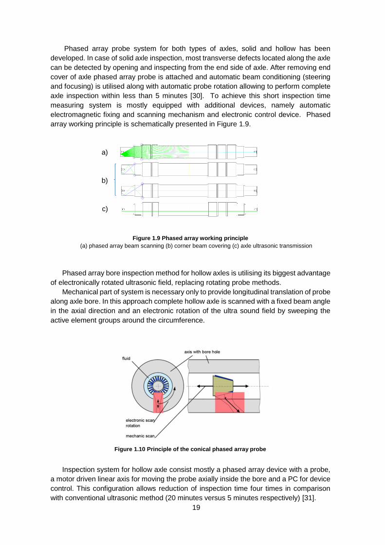
Phased array probe system for both types of axles, solid and hollow has been
developed. In case of solid axle inspection, most transverse defects located along the axle
can be detected by opening and inspecting from the end side of axle. After removing end
cover of axle phased array probe is attached and automatic beam conditioning (steering
and focusing) is utilised along with automatic probe rotation allowing to perform complete
axle inspection within less than 5 minutes [30]. To achieve this short inspection time
measuring system is mostly equipped with additional devices, namely automatic
electromagnetic fixing and scanning mechanism and electronic control device. Phased
array working principle is schematically presented in Figure 1.9.
a)
b)
c)
(a) phased array beam scanning (b) corner beam covering (c) axle ultrasonic transmission
Phased array bore inspection method for hollow axles is utilising its biggest advantage
of electronically rotated ultrasonic field, replacing rotating probe methods.
Mechanical part of system is necessary only to provide longitudinal translation of probe
along axle bore. In this approach complete hollow axle is scanned with a fixed beam angle
in the axial direction and an electronic rotation of the ultra sound field by sweeping the
active element groups around the circumference.
Inspection system for hollow axle consist mostly a phased array device with a probe,
a motor driven linear axis for moving the probe axially inside the bore and a PC for device
control. This configuration allows reduction of inspection time four times in comparison
with conventional ultrasonic method (20 minutes versus 5 minutes respectively) [31].
Figure 1.9 Phased array working principle
Figure 1.10 Principle of the conical phased array probe
20
Microwave sensor testing
This method is based on a physical phenomenon - the interaction of electron gas and
ultrasonic waves in metals. Emission of ultrasonic waves on the metal surface is
determined by microwave sensor. Theoretical works showed that there is possible fact to
determine remotely dangerous-or-non-dangerous inner metal stress, measuring the
surface conduction (density of surface charges)[32]. Research and testing were
conducted, including remote indicators of active defects on steel samples and railway
wheels in static mode, as well as, dynamic testing in moving mounted wheels.
Experiments showed that this new method could be used to determine the initial formation
of active defects (cracks), even under elastic tension.
One of the most important advantages of microwave method is the fact that it can be
used for detecting surface cracks under dielectric coatings. Because microwave signals
easily penetrate inside dielectric materials, this methodology is expected to detect cracks
under dielectric coatings of various thicknesses. It must be noted that dielectric coatings
such as paint, corrosion preventative substances, etc., may have varied thicknesses
although they are generally not very thick and are commonly known as the family of low-
loss dielectric materials.
AC thermography
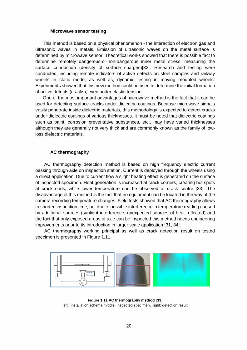
AC thermography detection method is based on high frequency electric current
passing through axle on inspection station. Current is deployed through the wheels using
a direct application. Due to current flow a slight heating effect is generated on the surface
of inspected specimen. Heat generation is increased at crack corners, creating hot spots
at crack ends, while lower temperature can be observed at crack centre [33]. The
disadvantage of this method is the fact that no equipment can be located in the way of the
camera recording temperature changes. Field tests showed that AC thermography allows
to shorten inspection time, but due to possible interference in temperature reading caused
by additional sources (sunlight interference, unexpected sources of heat reflected) and
the fact that only exposed areas of axle can be inspected this method needs engineering
improvements prior to its introduction in larger scale application [31, 34].
AC thermography working principal as well as crack detection result on tested
specimen is presented in Figure 1.11.
Figure 1.11 AC thermography method [33]
left: installation scheme middle: inspected specimen, right: detection result
21
Acoustic Emission (AE)
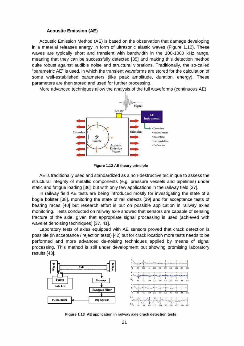
Acoustic Emission Method (AE) is based on the observation that damage developing
in a material releases energy in form of ultrasonic elastic waves (Figure 1.12). These
waves are typically short and transient with bandwidth in the 100-1000 kHz range,
meaning that they can be successfully detected [35] and making this detection method
quite robust against audible noise and structural vibrations. Traditionally, the so-called
“parametric AE” is used, in which the transient waveforms are stored for the calculation of
some well-established parameters (like peak amplitude, duration, energy). These
parameters are then stored and used for further processing.
More advanced techniques allow the analysis of the full waveforms (continuous AE).
Figure 1.12 AE theory principle
AE is traditionally used and standardized as a non-destructive technique to assess the
structural integrity of metallic components (e.g. pressure vessels and pipelines) under
static and fatigue loading [36], but with only few applications in the railway field [37].
In railway field AE tests are being introduced mostly for investigating the state of a
bogie bolster [38], monitoring the state of rail defects [39] and for acceptance tests of
bearing races [40] but research effort is put on possible application in railway axles
monitoring. Tests conducted on railway axle showed that sensors are capable of sensing
fracture of the axle, given that appropriate signal processing is used (achieved with
wavelet denoising techniques) [37, 41].
Laboratory tests of axles equipped with AE sensors proved that crack detection is
possible (in acceptance / rejection tests) [42] but for crack location more tests needs to be
performed and more advanced de-noising techniques applied by means of signal
processing. This method is still under development but showing promising laboratory
results [43].
Figure 1.13 AE application in railway axle crack detection tests
22
Laser-based ultrasonic cracked axle detection
This type of technology for crack axle detection utilises a laser in conjunction with
standard ultrasonic transducer to detect defects on the axle of train passing through a
testing station. A high-energy, pulsed laser is used to generate ultrasonic modes in a axle
and a non-contact, air-coupled transducer to receive the ultrasonic signal emitted by the
specimen which is then sent to a signal processing unit for analysis to determine the
presence of cracks across the axle circumference [44]. Each inspection is capable of
detecting circumferentially oriented cracks across the body of the axle. By repeating the
inspection multiple times around the circumference of the axle, it is possible to detect
cracks around the entire axle body. The automated cracked axle detection system consists
of 10 inspection stations, which inspect the axle for cracks greater than 7 [mm] long [29].
The system works at speeds up to 32 [km/h].
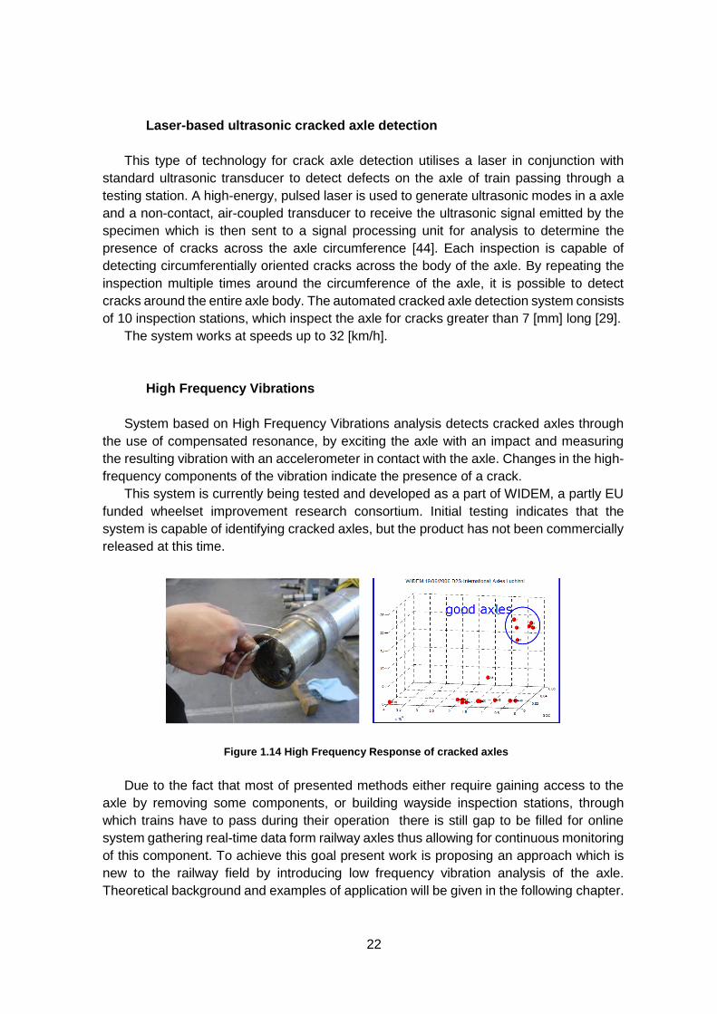
High Frequency Vibrations
System based on High Frequency Vibrations analysis detects cracked axles through
the use of compensated resonance, by exciting the axle with an impact and measuring
the resulting vibration with an accelerometer in contact with the axle. Changes in the high-
frequency components of the vibration indicate the presence of a crack.
This system is currently being tested and developed as a part of WIDEM, a partly EU
funded wheelset improvement research consortium. Initial testing indicates that the
system is capable of identifying cracked axles, but the product has not been commercially
released at this time.
Due to the fact that most of presented methods either require gaining access to the
axle by removing some components, or building wayside inspection stations, through
which trains have to pass during their operation there is still gap to be filled for online
system gathering real-time data form railway axles thus allowing for continuous monitoring
of this component. To achieve this goal present work is proposing an approach which is
new to the railway field by introducing low frequency vibration analysis of the axle.
Theoretical background and examples of application will be given in the following chapter.
Figure 1.14 High Frequency Response of cracked axles
23
CHAPTER 2
2. Crack-related vibrations in rotating shafts
Due to the fact that railway axle is a mechanical component operating under variable
loads and angular speeds, its behaviour falls into the wider field of dynamics of rotating
systems called rotordynamics. Condition monitoring of rotating systems has been an
active field of research during the past four decades. During this time rich database of
theoretical as well as experimental research has been created, as a result of demand for
reliable procedures that allows to detect and characterize fault condition of an operating
system without interrupting its normal working regime. Since generally any mechanical
component during operation passes through some degradation states before failure, if
such a condition can be detected in advance then proactive and corrective maintenance
can be applied before a complete failure occurs. This approach therefore, offers cost
savings compared to classical preventive activities which are performed periodically
without knowing if the component is really defective [45].
Among different strategies of estimating health condition of rotating elements, vibration
analysis is one which has many advantages. Vibrational signals can often be measured
by relatively inexpensive sensors (displacement proximity probes, accelerometers, etc.)
and what is most important, vibration signal of working system gives immediate evidence
of an eventual fault developing in its structure.
For characterising and analysing vibrational signal obtained from rotating components
different techniques of signal processing are used. Vibration analysis has been used for a
long time and already sophisticated techniques were developed over the last twenty years,
i.e. [46]
In general, the vibration signal contains the information of the oscillatory motion of the
machine and its auxiliary components. Each of the sub-components of rotating machinery,
like gears, bearings, shafts, couplings, engines, electric generators, pumps, fans, etc., can
be modelled so that the vibration from various modes of failure can be predicted [47]. The
goal of vibration signal processing is to analyse the vibration signal measured at particular
locations on the machine, and extract enough information to determine the condition of
each of the sub-elements of the machine.
Due to the fact that developing faults are giving response in specific range of angular
frequency of rotating component, very useful from diagnostic point of view is to observe
measured signal in the frequency domain. This can be achieved by applying an algorithm
well-defined in literature called Fourier Transform. The reference situation, where vibration
signal was recorded under normal (no fault) working condition of system is necessary in
any case, enabling comparison and trending of eventual changes in vibration signal
components. Trending of the Fourier transform frequency vectors itself, was
24
acknowledged to be useful for monitoring the condition of rotor shafts for the presence of
cracks [48].
Having proper, reliable, information coming from signal analysis, combined with
diagnostic experience or guidelines for system under consideration gives the possibility
for decision maker to correctly judge whether the system is acceptable for service or
maintenance should be planned.
2.1. Cracks in rotating shafts
Crack occurrence and its development are one of the most common causes of failure
in mechanical structures. Specifically, systems working under cyclic loading basis are
prone to this type of phenomena, which if not monitored can lead to complete failure of
elements in which crack was advancing.
As research done by many authors shows (some examples specifically for railway
axles were given in Chapter 1) crack may be initiated in areas with high stress
concentration (i.e. sharp changes of diameter of part geometry), surface imperfections
(including corrosion) and also due to material inclusions from which parts are being made.
Frequent source of crack initiation is fretting corrosion in case of shrink/press fitted
connections specifically when operating in wet and corrosive environments (i.e. railway
wheels).
Crack existence and its dimensions are investigated commonly by means of non-
destructive tests, i.e. dye penetrant, ultrasonic, MPI (brief description given in Section 1.4).
In case of shafts working in field of turbomachinery (i.e. power plants) dynamic tests,
based on vibration measurements are suggested for identifying presence and location of
cracks as the change in the overall dynamic behaviour might be caused by the local
reduction of the stiffness due to a crack that has developed somewhere in the structure
[49].
In rotating components like shafts, the most frequent type of crack appearance is so
called transverse crack, although its possible to find also slant, helicoidal, and multiple
cracks. Transverse cracks, are the type in which the crack surface is orthogonal to the
rotation axis of the shaft.
In general, crack existence is much harder to detect in case of rotating element during
its operation, especially when compared with stationary structures, thus vibrations
analysis have been found to be a suitable method to extract symptoms justifying
developing fault in a component under investigation. If these symptoms are found and
they are giving the right to suspect fault existence which is putting threat to system safe
operation, then maintenance activities might be planned with minimised disturbance in
machine working schedule.
2.1.1. Crack propagation in rotating shafts
Research on crack initiation and propagation phenomena generally falls into the field
of fracture-mechanics. More accurate models are continuously developed to investigate
crack propagation paths and speeds [25, 50] which are giving possibility to better design
or predict components life prone to crack occurrences.
25
Since the most successful approach to the study of fatigue crack propagation is based
on fracture-mechanics concepts thus in case of crack investigation in rotating elements
fracture mechanics along with rotordynamics play key role in modelling, analyzing, and
interpreting results of analysis.
During extensive studies of cracking phenomena done by many authors it has been
shown that high stress intensity factors are developing at the crack tip and thus allow the
crack to propagate deeper inside element structure, even if the external loads are not
changing. The crack propagation path is generally determined by the direction of
maximum stress or by the minimum material strength. The crack can propagate slowly at
the beginning, often with periods of rest alternating with periods of propagation, but as
soon as the crack will reach a relevant depth, then the propagation speed increases
dramatically and the shaft may fail in short time of operation. At the initial stage of crack
propagation the propagation direction is depending on local conditions thus it can follow
virtually any direction. The situation changes as soon as the crack reaches the deeper
regions of the structure when the direction of propagation is happening mainly in radial
direction with small vanishing curvatures. When a cracked element is loaded with constant
amplitude its very often visible that crack propagates in steps, creating specific cracked
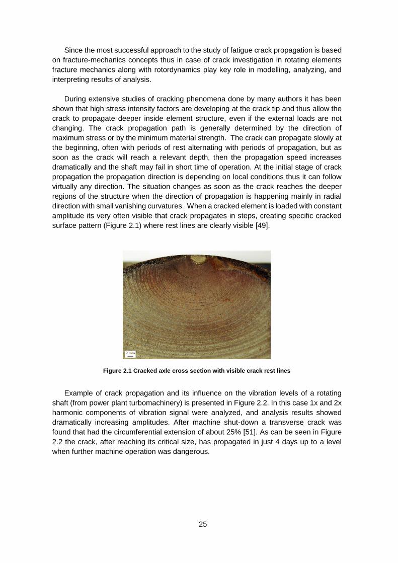
surface pattern (Figure 2.1) where rest lines are clearly visible [49].
Figure 2.1 Cracked axle cross section with visible crack rest lines
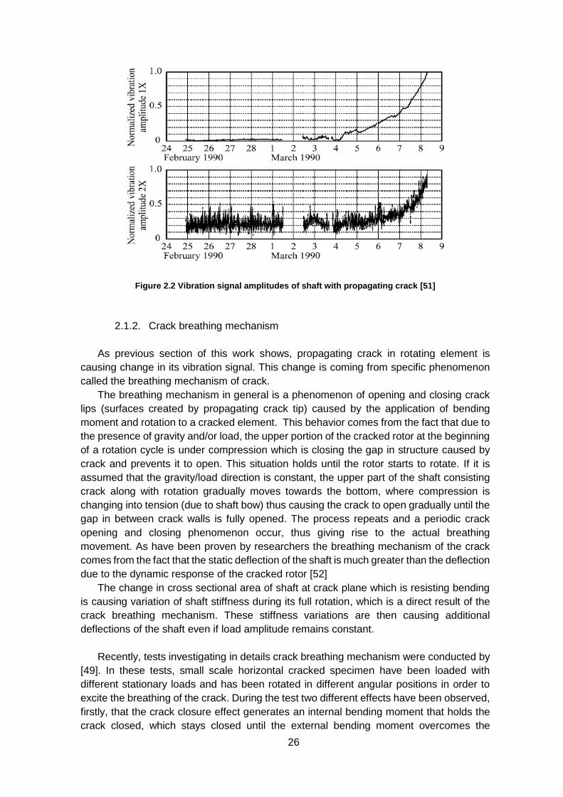
Example of crack propagation and its influence on the vibration levels of a rotating
shaft (from power plant turbomachinery) is presented in Figure 2.2. In this case 1x and 2x
harmonic components of vibration signal were analyzed, and analysis results showed
dramatically increasing amplitudes. After machine shut-down a transverse crack was
found that had the circumferential extension of about 25% [51]. As can be seen in Figure
2.2 the crack, after reaching its critical size, has propagated in just 4 days up to a level
when further machine operation was dangerous.
26
Figure 2.2 Vibration signal amplitudes of shaft with propagating crack [51]
2.1.2. Crack breathing mechanism
As previous section of this work shows, propagating crack in rotating element is
causing change in its vibration signal. This change is coming from specific phenomenon
called the breathing mechanism of crack.
The breathing mechanism in general is a phenomenon of opening and closing crack
lips (surfaces created by propagating crack tip) caused by the application of bending
moment and rotation to a cracked element. This behavior comes from the fact that due to
the presence of gravity and/or load, the upper portion of the cracked rotor at the beginning
of a rotation cycle is under compression which is closing the gap in structure caused by
crack and prevents it to open. This situation holds until the rotor starts to rotate. If it is
assumed that the gravity/load direction is constant, the upper part of the shaft consisting
crack along with rotation gradually moves towards the bottom, where compression is
changing into tension (due to shaft bow) thus causing the crack to open gradually until the
gap in between crack walls is fully opened. The process repeats and a periodic crack
opening and closing phenomenon occur, thus giving rise to the actual breathing
movement. As have been proven by researchers the breathing mechanism of the crack
comes from the fact that the static deflection of the shaft is much greater than the deflection
due to the dynamic response of the cracked rotor [52]
The change in cross sectional area of shaft at crack plane which is resisting bending
is causing variation of shaft stiffness during its full rotation, which is a direct result of the
crack breathing mechanism. These stiffness variations are then causing additional
deflections of the shaft even if load amplitude remains constant.
Recently, tests investigating in details crack breathing mechanism were conducted by
[49]. In these tests, small scale horizontal cracked specimen have been loaded with
different stationary loads and has been rotated in different angular positions in order to
excite the breathing of the crack. During the test two different effects have been observed,
firstly, that the crack closure effect generates an internal bending moment that holds the
crack closed, which stays closed until the external bending moment overcomes the
27
internal bending moment, and secondly that when the crack is closed the measured
compressive strain is much higher than the theoretical strain calculated assuming a linear
compressive stress distribution over the cracked section. This was explained by assuming
that the contact is not spread over all the cracked area when the crack is closed, but it
occurs only on a smaller portion of the cracked surface, or on the crack lips only,
determining higher strains associated also to stress intensity factors. This aspect is also
related to the crack closure effect.
As can be understood the breathing mechanism is the result of the stress and strain
distribution around the cracked area, due to static loads (weight, reaction forces, etc.) and
dynamical loads (i.e. unbalance). As experiment results are showing [49] as long as static
loads are overcoming the dynamical ones, the breathing is governed by the angular
position of the shaft with respect to the stationary load direction. In this configuration crack
opens and closes completely once per revolution of shaft.
Important conclusion after observing the crack breathing mechanism and its influence
on structure was that despite the highly non-linear stress and strain distribution in the
cracked area and the non-linear breathing behaviour, the overall load-strain behaviour of
rotating shaft resulted to be quite linear.
Although some authors [53] were assuming an abrupt change of crack condition from
completely open state to completely close state, detailed investigation of crack breathing
mechanism done by further research proved that this situation is unusual in real
applications. Effect of gradually closing and opening crack lips is more closely
representing crack breathing phenomena of real shafts. This fact was confirmed also by
the use of finite element models to investigate crack influence on train axle, which is the
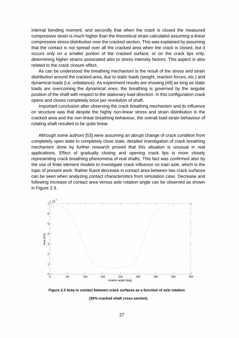
topic of present work. Rather fluent decrease in contact area between two crack surfaces
can be seen when analyzing contact characteristics from simulation case. Decrease and
following increase of contact area versus axle rotation angle can be observed as shown
in Figure 2.3.
(35% cracked shaft cross section)
0 50 100 150 200 250 300 350 4000
1
2
3
4
5
6
7x 10
-3
rotation angle [deg]
are
a [
m2]
Figure 2.3 Area in contact between crack surfaces as a function of axle rotation
28
2.1.3. Dynamic behavior of cracked shafts
Proper assessment of whether or not a rotating shaft is operating in healthy condition
requires knowledge of its dynamic behavior. To describe and understand dynamics of a
cracked shaft both rotordynamics as well as fracture mechanics concepts are playing key
role. Due to the fact that both of these fields of science are wide, but also well defined in
literature, this section will focus on the review of the influence of crack on the vibrational
signal, thus giving insight to understanding results of vibrational signal analysis.
A crack in the rotor causes local change in stiffness, which than affects the dynamics
of the system: frequency of the natural vibrations and the amplitudes of forced vibrations
are changed. The influence of a transverse crack on the vibration of a rotating shaft has
been studied by researchers since three decades. Wide review of crack modeling,
understanding the behavior of cracked shafts as well as crack localization techniques was
widely contributed mainly by [48, 54-57]. More recent studies have been published by [58].
As was already stated, apart from the overall level of vibration, vibration signal
harmonics are offering great diagnostic information. Due to the fact that every sub-element
of a rotating system generates a vibration specific pattern (i.e. gears, bearings, etc.) in
specific range of frequency, analysis in frequency domain is very useful from diagnose
point of view. In cracked rotating shafts, crack presence has peculiar influence on dynamic
behavior of the shaft due to the breathing mechanism occurring during each revolution of
shaft. By analyzing the harmonic components of vibration signal recorded from a cracked
shaft some observations can be made. According to [49] when deflections are measured
along the shaft loaded by its weight during a complete revolution of the shaft, the Fourier
expansion allows the definition of 1X, 2X and 3X deflection shapes. All are due to the local
flexibility of the crack only and have therefore a bi-linear shape with a pronounced
curvature in correspondence of the crack. Therefore some typical symptoms of crack
influence on shaft dynamic behaviour can be observed, namely a change in 1X, 2X and
3X vibration signal harmonic [59-62].
A brief summary of common changes and its causes can be made based on literature
[49, 50] specifically:
- the 1X component is increasing mostly due to the development of the bow caused
by the crack, however also can be caused by many other faults (e.g. unbalance,
coupling misalignments, etc.), so attention needs to be paid when taking diagnostic
decision;
- the 2X component is mostly changing amplitude because of axial asymmetry in
rotating shaft due to fault, but also can be caused by surface geometry errors
(journal ovalisation) and intrinsic stiffness asymmetry in case of asymmetric shaft
that could cause 2X vibration component also during normal operating, which has
to be treated as machine native vibrations;
- the 3X harmonic component is mostly caused by a breathing crack mechanism,
but this excitation is rather small and can be recognized only when resonance
amplifies the response. It’s necessary to note that 3X components can also be
caused by surface geometry errors (journal ovalisation). In some cases it was
29
observed that 3X component didn’t change its amplitude even if deep crack were
present in shaft, which was coming from the fact that crack was permanently
opened, thus no breathing mechanism occurred [63].
Examples are mostly showing that the presence of a crack caused a remarkable
change in the normal vibration level of the machines [51, 64, 65].
It is worth emphasizing, that not only an increase of the harmonic components can
indicate the presence of a crack. Examples of decreasing spectra amplitudes due to crack
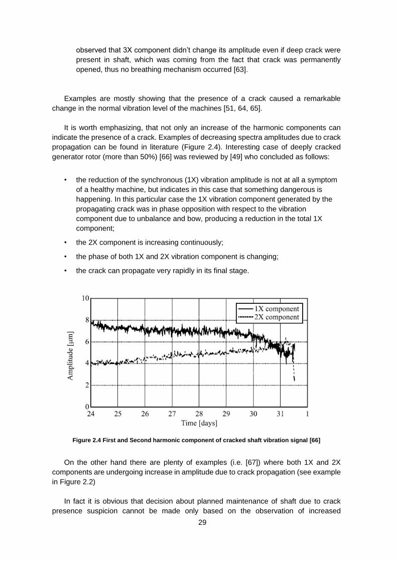
propagation can be found in literature (Figure 2.4). Interesting case of deeply cracked
generator rotor (more than 50%) [66] was reviewed by [49] who concluded as follows:
• the reduction of the synchronous (1X) vibration amplitude is not at all a symptom
of a healthy machine, but indicates in this case that something dangerous is
happening. In this particular case the 1X vibration component generated by the
propagating crack was in phase opposition with respect to the vibration
component due to unbalance and bow, producing a reduction in the total 1X
component;
• the 2X component is increasing continuously;
• the phase of both 1X and 2X vibration component is changing;
• the crack can propagate very rapidly in its final stage.
Figure 2.4 First and Second harmonic component of cracked shaft vibration signal [66]
On the other hand there are plenty of examples (i.e. [67]) where both 1X and 2X
components are undergoing increase in amplitude due to crack propagation (see example
in Figure 2.2)
In fact it is obvious that decision about planned maintenance of shaft due to crack
presence suspicion cannot be made only based on the observation of increased
30
amplitudes of specific harmonics (mostly 1X to 3X) but rather based on the rate of change
of their amplitudes.
Generally, if comparison with stationary structures could be made, rotating shafts have
some special characteristics. First one is coming directly from the crack breathing
phenomena, which is independent from the vibration. In rotating components crack is
opening and closing gradually, while in stationary structures this change is rather abrupt,
due to character of applied external forces. Second important characteristic is the fact that
vibrations originated from crack in rotating components are excited naturally by the rotation
of shaft (breathing phenomena), thus periodicity is much more expected, while in
stationary structures these vibrations are excited by external forces.
As [68] concluded, after extensive literature review and own experiments, in case of
rotating shafts 2X component trend analysis is the best tool for discovering a crack. It
comes in line with other works, i.e. [60], where nonlinear dynamic behaviour of the cracked
rotor was investigated experimentally and authors also observed higher harmonics
(especially 2X frequency component) in the response of the cracked rotor, when the rotor
is running in the subcritical speed range (below the angular frequency that causes a
resonance).
Due to the fact that obviously vibration measurements are giving sufficient information
to estimate crack occurrence, and that specific crack-related vibrations characteristics
depend directly on crack breathing phenomena (thus crack size and location) the
importance of adequate modeling of crack zone is essential in case of numerical
simulations of cracked shaft dynamical behavior.
2.2. Crack modelling
Accurate modelling of the cracked shaft allows to simulate its dynamic behavior,
including influence of crack different location, size and shape. The comparison of
calculated vibrations and measured vibrations allows the identification of not only the
presence of a crack in a rotating shaft, but also of its location and depth, using a diagnostic
procedure [59], thus having available a correct model of crack zone is essential for a
research process. Some popular crack models will be briefly introduced in following
subsection.
2.2.1. Types of crack models used in simulations
Nonlinear dynamics of the cracked rotor is mostly investigated using two well-known
crack models, i.e. switching crack model and response-dependent breathing crack model.
Switching crack model was developed following the fact that the transition from closed
crack (full) stiffness to the open crack (weak) stiffness has been generally considered
abrupt [53]. This model was easier to implement mathematically but further investigations
revealed its disadvantages. In real cracked rotors, the stiffness variation is likely to be
gradual, the assumption of abrupt stiffness switching is not appropriate. Hence, the
switching crack model might adequately represent only very shallow cracks. [52] proved
that switching crack modelling reveals chaotic, quasi-periodic and subharmonic vibration
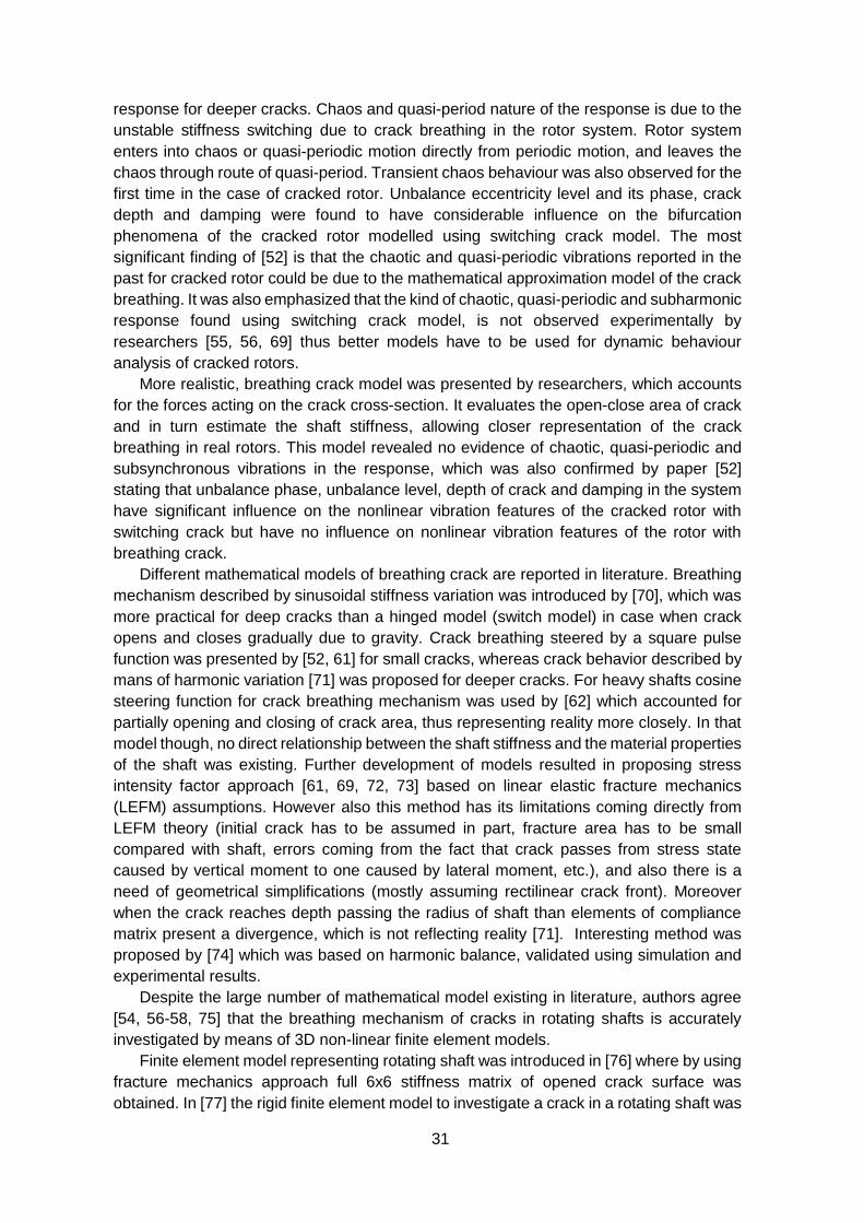
31
response for deeper cracks. Chaos and quasi-period nature of the response is due to the
unstable stiffness switching due to crack breathing in the rotor system. Rotor system
enters into chaos or quasi-periodic motion directly from periodic motion, and leaves the
chaos through route of quasi-period. Transient chaos behaviour was also observed for the
first time in the case of cracked rotor. Unbalance eccentricity level and its phase, crack
depth and damping were found to have considerable influence on the bifurcation
phenomena of the cracked rotor modelled using switching crack model. The most
significant finding of [52] is that the chaotic and quasi-periodic vibrations reported in the
past for cracked rotor could be due to the mathematical approximation model of the crack
breathing. It was also emphasized that the kind of chaotic, quasi-periodic and subharmonic
response found using switching crack model, is not observed experimentally by
researchers [55, 56, 69] thus better models have to be used for dynamic behaviour
analysis of cracked rotors.
More realistic, breathing crack model was presented by researchers, which accounts
for the forces acting on the crack cross-section. It evaluates the open-close area of crack
and in turn estimate the shaft stiffness, allowing closer representation of the crack
breathing in real rotors. This model revealed no evidence of chaotic, quasi-periodic and
subsynchronous vibrations in the response, which was also confirmed by paper [52]
stating that unbalance phase, unbalance level, depth of crack and damping in the system
have significant influence on the nonlinear vibration features of the cracked rotor with
switching crack but have no influence on nonlinear vibration features of the rotor with
breathing crack.
Different mathematical models of breathing crack are reported in literature. Breathing
mechanism described by sinusoidal stiffness variation was introduced by [70], which was
more practical for deep cracks than a hinged model (switch model) in case when crack
opens and closes gradually due to gravity. Crack breathing steered by a square pulse
function was presented by [52, 61] for small cracks, whereas crack behavior described by
mans of harmonic variation [71] was proposed for deeper cracks. For heavy shafts cosine
steering function for crack breathing mechanism was used by [62] which accounted for
partially opening and closing of crack area, thus representing reality more closely. In that
model though, no direct relationship between the shaft stiffness and the material properties
of the shaft was existing. Further development of models resulted in proposing stress
intensity factor approach [61, 69, 72, 73] based on linear elastic fracture mechanics
(LEFM) assumptions. However also this method has its limitations coming directly from
LEFM theory (initial crack has to be assumed in part, fracture area has to be small
compared with shaft, errors coming from the fact that crack passes from stress state
caused by vertical moment to one caused by lateral moment, etc.), and also there is a
need of geometrical simplifications (mostly assuming rectilinear crack front). Moreover
when the crack reaches depth passing the radius of shaft than elements of compliance
matrix present a divergence, which is not reflecting reality [71]. Interesting method was
proposed by [74] which was based on harmonic balance, validated using simulation and
experimental results.
Despite the large number of mathematical model existing in literature, authors agree
[54, 56-58, 75] that the breathing mechanism of cracks in rotating shafts is accurately
investigated by means of 3D non-linear finite element models.
Finite element model representing rotating shaft was introduced in [76] where by using
fracture mechanics approach full 6x6 stiffness matrix of opened crack surface was
obtained. In [77] the rigid finite element model to investigate a crack in a rotating shaft was
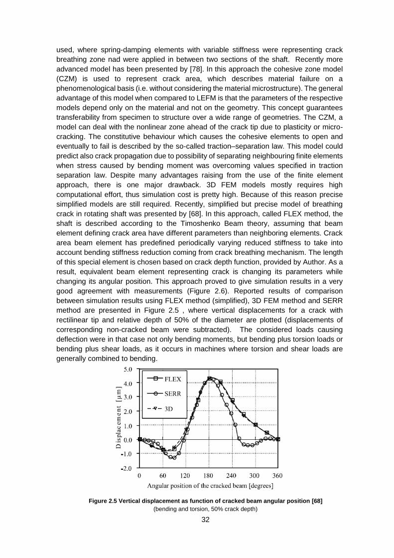
32
used, where spring-damping elements with variable stiffness were representing crack
breathing zone nad were applied in between two sections of the shaft. Recently more
advanced model has been presented by [78]. In this approach the cohesive zone model
(CZM) is used to represent crack area, which describes material failure on a
phenomenological basis (i.e. without considering the material microstructure). The general
advantage of this model when compared to LEFM is that the parameters of the respective
models depend only on the material and not on the geometry. This concept guarantees
transferability from specimen to structure over a wide range of geometries. The CZM, a
model can deal with the nonlinear zone ahead of the crack tip due to plasticity or micro-
cracking. The constitutive behaviour which causes the cohesive elements to open and
eventually to fail is described by the so-called traction–separation law. This model could
predict also crack propagation due to possibility of separating neighbouring finite elements
when stress caused by bending moment was overcoming values specified in traction
separation law. Despite many advantages raising from the use of the finite element
approach, there is one major drawback. 3D FEM models mostly requires high
computational effort, thus simulation cost is pretty high. Because of this reason precise
simplified models are still required. Recently, simplified but precise model of breathing
crack in rotating shaft was presented by [68]. In this approach, called FLEX method, the
shaft is described according to the Timoshenko Beam theory, assuming that beam
element defining crack area have different parameters than neighboring elements. Crack
area beam element has predefined periodically varying reduced stiffness to take into
account bending stiffness reduction coming from crack breathing mechanism. The length
of this special element is chosen based on crack depth function, provided by Author. As a
result, equivalent beam element representing crack is changing its parameters while
changing its angular position. This approach proved to give simulation results in a very
good agreement with measurements (Figure 2.6). Reported results of comparison
between simulation results using FLEX method (simplified), 3D FEM method and SERR
method are presented in Figure 2.5 , where vertical displacements for a crack with
rectilinear tip and relative depth of 50% of the diameter are plotted (displacements of
corresponding non-cracked beam were subtracted). The considered loads causing
deflection were in that case not only bending moments, but bending plus torsion loads or
bending plus shear loads, as it occurs in machines where torsion and shear loads are
generally combined to bending.
Figure 2.5 Vertical displacement as function of cracked beam angular position [68]
(bending and torsion, 50% crack depth)
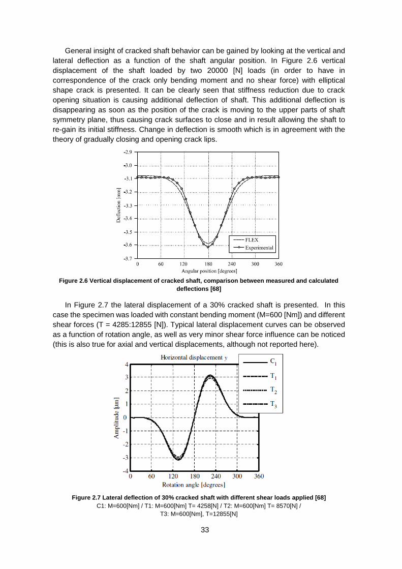
33
General insight of cracked shaft behavior can be gained by looking at the vertical and
lateral deflection as a function of the shaft angular position. In Figure 2.6 vertical
displacement of the shaft loaded by two 20000 [N] loads (in order to have in
correspondence of the crack only bending moment and no shear force) with elliptical
shape crack is presented. It can be clearly seen that stiffness reduction due to crack
opening situation is causing additional deflection of shaft. This additional deflection is
disappearing as soon as the position of the crack is moving to the upper parts of shaft
symmetry plane, thus causing crack surfaces to close and in result allowing the shaft to
re-gain its initial stiffness. Change in deflection is smooth which is in agreement with the
theory of gradually closing and opening crack lips.
Figure 2.6 Vertical displacement of cracked shaft, comparison between measured and calculated
deflections [68]
In Figure 2.7 the lateral displacement of a 30% cracked shaft is presented. In this
case the specimen was loaded with constant bending moment (M=600 [Nm]) and different
shear forces (T = 4285:12855 [N]). Typical lateral displacement curves can be observed
as a function of rotation angle, as well as very minor shear force influence can be noticed
(this is also true for axial and vertical displacements, although not reported here).
Figure 2.7 Lateral deflection of 30% cracked shaft with different shear loads applied [68]
C1: M=600[Nm] / T1: M=600[Nm] T= 4258[N] / T2: M=600[Nm] T= 8570[N] /
T3: M=600[Nm], T=12855[N]
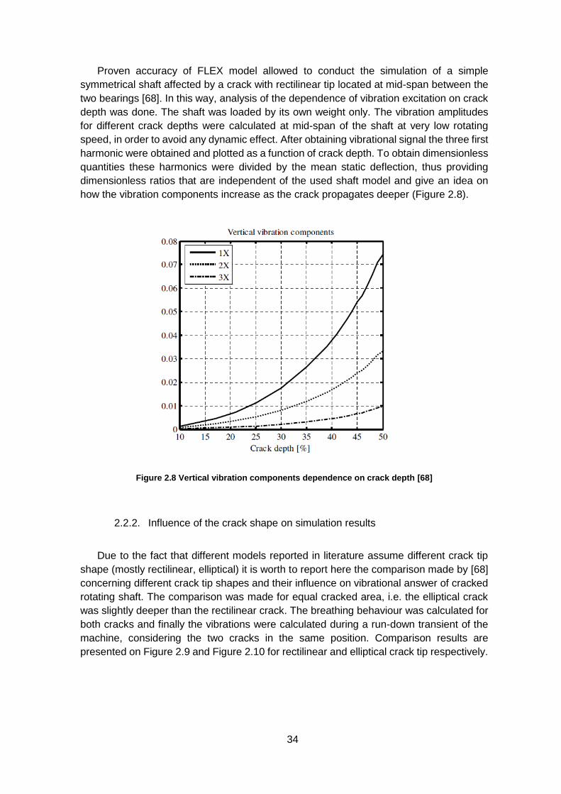
34
Proven accuracy of FLEX model allowed to conduct the simulation of a simple
symmetrical shaft affected by a crack with rectilinear tip located at mid-span between the
two bearings [68]. In this way, analysis of the dependence of vibration excitation on crack
depth was done. The shaft was loaded by its own weight only. The vibration amplitudes
for different crack depths were calculated at mid-span of the shaft at very low rotating
speed, in order to avoid any dynamic effect. After obtaining vibrational signal the three first
harmonic were obtained and plotted as a function of crack depth. To obtain dimensionless
quantities these harmonics were divided by the mean static deflection, thus providing
dimensionless ratios that are independent of the used shaft model and give an idea on
how the vibration components increase as the crack propagates deeper (Figure 2.8).
Figure 2.8 Vertical vibration components dependence on crack depth [68]
2.2.2. Influence of the crack shape on simulation results
Due to the fact that different models reported in literature assume different crack tip
shape (mostly rectilinear, elliptical) it is worth to report here the comparison made by [68]
concerning different crack tip shapes and their influence on vibrational answer of cracked
rotating shaft. The comparison was made for equal cracked area, i.e. the elliptical crack
was slightly deeper than the rectilinear crack. The breathing behaviour was calculated for
both cracks and finally the vibrations were calculated during a run-down transient of the
machine, considering the two cracks in the same position. Comparison results are
presented on Figure 2.9 and Figure 2.10 for rectilinear and elliptical crack tip respectively.
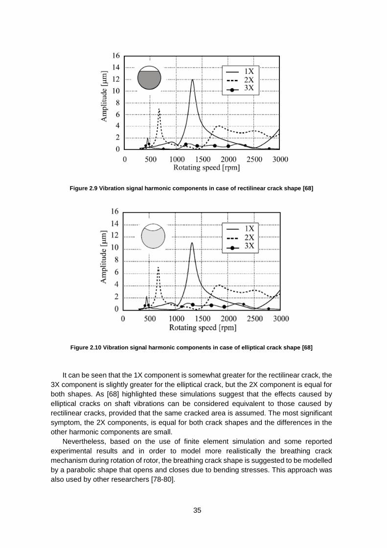
35
Figure 2.9 Vibration signal harmonic components in case of rectilinear crack shape [68]
Figure 2.10 Vibration signal harmonic components in case of elliptical crack shape [68]
It can be seen that the 1X component is somewhat greater for the rectilinear crack, the
3X component is slightly greater for the elliptical crack, but the 2X component is equal for
both shapes. As [68] highlighted these simulations suggest that the effects caused by
elliptical cracks on shaft vibrations can be considered equivalent to those caused by
rectilinear cracks, provided that the same cracked area is assumed. The most significant
symptom, the 2X components, is equal for both crack shapes and the differences in the
other harmonic components are small.
Nevertheless, based on the use of finite element simulation and some reported
experimental results and in order to model more realistically the breathing crack
mechanism during rotation of rotor, the breathing crack shape is suggested to be modelled
by a parabolic shape that opens and closes due to bending stresses. This approach was
also used by other researchers [78-80].
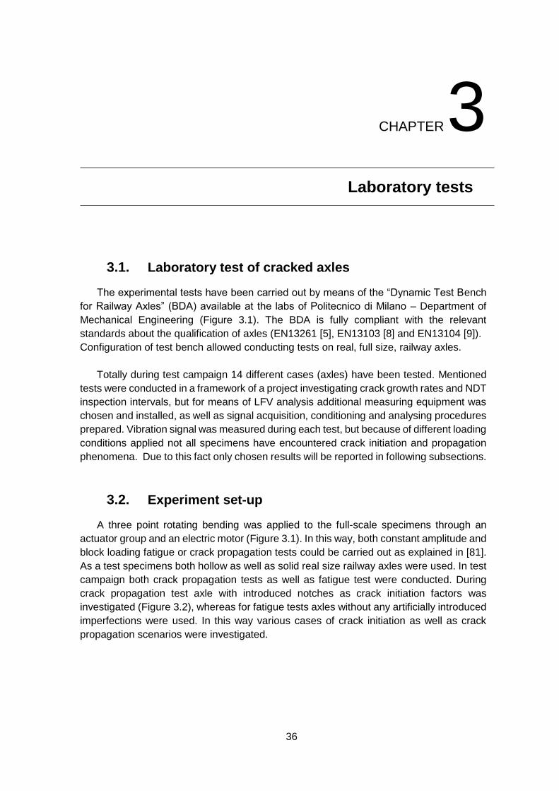
36
CHAPTER 3
3. Laboratory tests
3.1. Laboratory test of cracked axles
The experimental tests have been carried out by means of the “Dynamic Test Bench
for Railway Axles” (BDA) available at the labs of Politecnico di Milano – Department of
Mechanical Engineering (Figure 3.1). The BDA is fully compliant with the relevant
standards about the qualification of axles (EN13261 [5], EN13103 [8] and EN13104 [9]).
Configuration of test bench allowed conducting tests on real, full size, railway axles.
Totally during test campaign 14 different cases (axles) have been tested. Mentioned
tests were conducted in a framework of a project investigating crack growth rates and NDT
inspection intervals, but for means of LFV analysis additional measuring equipment was
chosen and installed, as well as signal acquisition, conditioning and analysing procedures
prepared. Vibration signal was measured during each test, but because of different loading
conditions applied not all specimens have encountered crack initiation and propagation
phenomena. Due to this fact only chosen results will be reported in following subsections.
3.2. Experiment set-up
A three point rotating bending was applied to the full-scale specimens through an
actuator group and an electric motor (Figure 3.1). In this way, both constant amplitude and
block loading fatigue or crack propagation tests could be carried out as explained in [81].
As a test specimens both hollow as well as solid real size railway axles were used. In test
campaign both crack propagation tests as well as fatigue test were conducted. During
crack propagation test axle with introduced notches as crack initiation factors was
investigated (Figure 3.2), whereas for fatigue tests axles without any artificially introduced
imperfections were used. In this way various cases of crack initiation as well as crack
propagation scenarios were investigated.
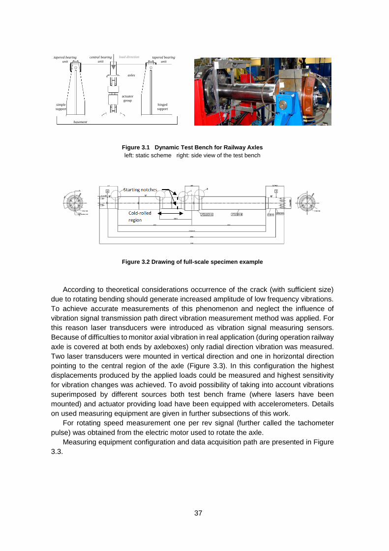
37
Figure 3.1 Dynamic Test Bench for Railway Axles
left: static scheme right: side view of the test bench
Figure 3.2 Drawing of full-scale specimen example
According to theoretical considerations occurrence of the crack (with sufficient size)
due to rotating bending should generate increased amplitude of low frequency vibrations.
To achieve accurate measurements of this phenomenon and neglect the influence of
vibration signal transmission path direct vibration measurement method was applied. For
this reason laser transducers were introduced as vibration signal measuring sensors.
Because of difficulties to monitor axial vibration in real application (during operation railway
axle is covered at both ends by axleboxes) only radial direction vibration was measured.
Two laser transducers were mounted in vertical direction and one in horizontal direction
pointing to the central region of the axle (Figure 3.3). In this configuration the highest
displacements produced by the applied loads could be measured and highest sensitivity
for vibration changes was achieved. To avoid possibility of taking into account vibrations
superimposed by different sources both test bench frame (where lasers have been
mounted) and actuator providing load have been equipped with accelerometers. Details
on used measuring equipment are given in further subsections of this work.
For rotating speed measurement one per rev signal (further called the tachometer
pulse) was obtained from the electric motor used to rotate the axle.
Measuring equipment configuration and data acquisition path are presented in Figure
3.3.
simple
support
hinged
support
actuator
group
basement
axles
tapered bearing
unit
tapered bearing
unit
central bearing
unit
load direction
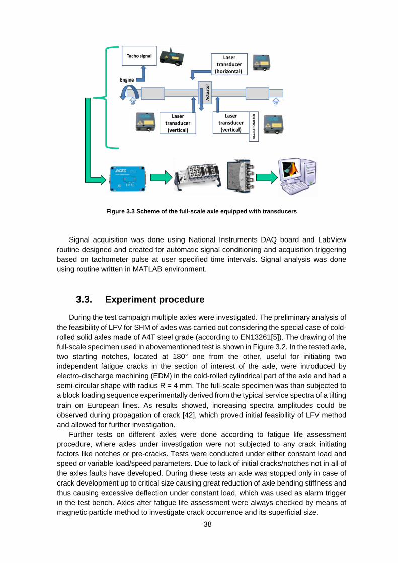
38
Figure 3.3 Scheme of the full-scale axle equipped with transducers
Signal acquisition was done using National Instruments DAQ board and LabView
routine designed and created for automatic signal conditioning and acquisition triggering
based on tachometer pulse at user specified time intervals. Signal analysis was done
using routine written in MATLAB environment.
3.3. Experiment procedure
During the test campaign multiple axles were investigated. The preliminary analysis of
the feasibility of LFV for SHM of axles was carried out considering the special case of cold-
rolled solid axles made of A4T steel grade (according to EN13261[5]). The drawing of the
full-scale specimen used in abovementioned test is shown in Figure 3.2. In the tested axle,
two starting notches, located at 180° one from the other, useful for initiating two
independent fatigue cracks in the section of interest of the axle, were introduced by
electro-discharge machining (EDM) in the cold-rolled cylindrical part of the axle and had a
semi-circular shape with radius R = 4 mm. The full-scale specimen was than subjected to
a block loading sequence experimentally derived from the typical service spectra of a tilting
train on European lines. As results showed, increasing spectra amplitudes could be
observed during propagation of crack [42], which proved initial feasibility of LFV method
and allowed for further investigation.
Further tests on different axles were done according to fatigue life assessment
procedure, where axles under investigation were not subjected to any crack initiating
factors like notches or pre-cracks. Tests were conducted under either constant load and
speed or variable load/speed parameters. Due to lack of initial cracks/notches not in all of
the axles faults have developed. During these tests an axle was stopped only in case of
crack development up to critical size causing great reduction of axle bending stiffness and
thus causing excessive deflection under constant load, which was used as alarm trigger
in the test bench. Axles after fatigue life assessment were always checked by means of
magnetic particle method to investigate crack occurrence and its superficial size.
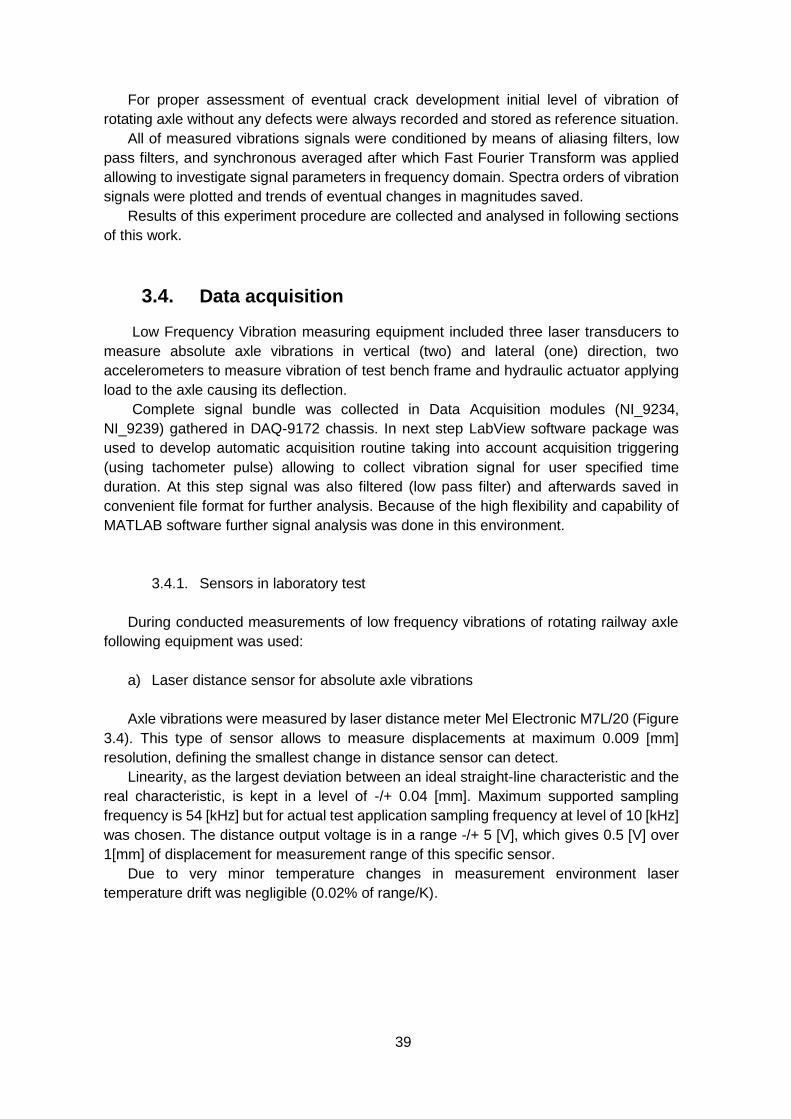
39
For proper assessment of eventual crack development initial level of vibration of
rotating axle without any defects were always recorded and stored as reference situation.
All of measured vibrations signals were conditioned by means of aliasing filters, low
pass filters, and synchronous averaged after which Fast Fourier Transform was applied
allowing to investigate signal parameters in frequency domain. Spectra orders of vibration
signals were plotted and trends of eventual changes in magnitudes saved.
Results of this experiment procedure are collected and analysed in following sections
of this work.
3.4. Data acquisition
Low Frequency Vibration measuring equipment included three laser transducers to
measure absolute axle vibrations in vertical (two) and lateral (one) direction, two
accelerometers to measure vibration of test bench frame and hydraulic actuator applying
load to the axle causing its deflection.
Complete signal bundle was collected in Data Acquisition modules (NI_9234,
NI_9239) gathered in DAQ-9172 chassis. In next step LabView software package was
used to develop automatic acquisition routine taking into account acquisition triggering
(using tachometer pulse) allowing to collect vibration signal for user specified time
duration. At this step signal was also filtered (low pass filter) and afterwards saved in
convenient file format for further analysis. Because of the high flexibility and capability of
MATLAB software further signal analysis was done in this environment.
3.4.1. Sensors in laboratory test
During conducted measurements of low frequency vibrations of rotating railway axle
following equipment was used:
a) Laser distance sensor for absolute axle vibrations
Axle vibrations were measured by laser distance meter Mel Electronic M7L/20 (Figure
3.4). This type of sensor allows to measure displacements at maximum 0.009 [mm]
resolution, defining the smallest change in distance sensor can detect.
Linearity, as the largest deviation between an ideal straight-line characteristic and the
real characteristic, is kept in a level of -/+ 0.04 [mm]. Maximum supported sampling
frequency is 54 [kHz] but for actual test application sampling frequency at level of 10 [kHz]
was chosen. The distance output voltage is in a range -/+ 5 [V], which gives 0.5 [V] over
1[mm] of displacement for measurement range of this specific sensor.
Due to very minor temperature changes in measurement environment laser
temperature drift was negligible (0.02% of range/K).

40
Figure 3.4 Laser sensor head and main control unit
credit: Mel Electronics
b) Accelerometers for external source vibration measurements
Due to the fact that additional testing devices are used in the same laboratory where
the vibrations measurements of axles were conducted it was necessary to ensure that no
other source of vibration is influencing measured signals. For this reason accelerometer
was mounted at the test bench frame, measuring total vibration of test bench rigidly
connected to the foundation. In this way possible transient vibrations originating from
different sources than rotating axle could be detected. Bending load, simulating loads
coming from real train, was applied to the axle by means of hydraulic actuator at centre of
axle. Because of that any deviation of force value generated by this unit had direct effect
on deflection of axle. To be able to measure possible vibrations generated by hydraulic
actuator accelerometer was mounted at the actuator head, and additionally force value of
actuator was stored along with vibration data.
Accelerometers used during the test were of type 4508 DeltaTron, with measurement
frequency range 0.3 [Hz] to 8 [kHz] (Amplitude), and measuring range -/+700 ms-2 peak (-
/+ 71g peak).
Signals measured by accelerometers were analysed and during whole mentioned axle
tests no additional sources of vibration have been found which could possibly influence
low frequency vibration generated by rotating axle.
c) Laser transducers acquisition module
Signal measured by laser transducers was collected by means of acquisition module
NI 9234 (Figure 3.5a). This is an AC/DC Analog Input dynamic signal acquisition module
for making high-accuracy measurements. It was specifically designed for high-channel-
count sound and vibration applications [82]. The four input channels of this module are
capable of simultaneously digitize signals at rates up to 51.2 [kHz] per channel with built-
in anti-aliasing filters that automatically adjust to specified sampling rate. This module
offers 24-bit resolution and 102 [dB] dynamic range.
Sampling rate value chosen for measuring axle vibrations (10 kHz) was applied to
each of module channel. It was possible due to the fact that analog-digital converters
(ADC’s) used in this acquisition module are channel-dedicated and user specified
sampling rate value is not divided by number of channels (as it happens when device
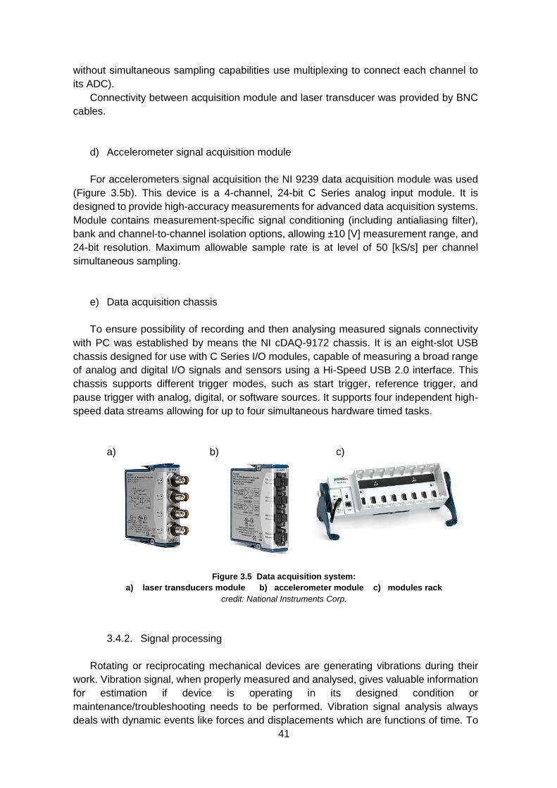
41
without simultaneous sampling capabilities use multiplexing to connect each channel to
its ADC).
Connectivity between acquisition module and laser transducer was provided by BNC
cables.
d) Accelerometer signal acquisition module
For accelerometers signal acquisition the NI 9239 data acquisition module was used
(Figure 3.5b). This device is a 4-channel, 24-bit C Series analog input module. It is
designed to provide high-accuracy measurements for advanced data acquisition systems.
Module contains measurement-specific signal conditioning (including antialiasing filter),
bank and channel-to-channel isolation options, allowing ±10 [V] measurement range, and
24-bit resolution. Maximum allowable sample rate is at level of 50 [kS/s] per channel
simultaneous sampling.
e) Data acquisition chassis
To ensure possibility of recording and then analysing measured signals connectivity
with PC was established by means the NI cDAQ-9172 chassis. It is an eight-slot USB
chassis designed for use with C Series I/O modules, capable of measuring a broad range
of analog and digital I/O signals and sensors using a Hi-Speed USB 2.0 interface. This
chassis supports different trigger modes, such as start trigger, reference trigger, and
pause trigger with analog, digital, or software sources. It supports four independent high-
speed data streams allowing for up to four simultaneous hardware timed tasks.
a) b) c)
Figure 3.5 Data acquisition system:
a) laser transducers module b) accelerometer module c) modules rack
credit: National Instruments Corp.
3.4.2. Signal processing
Rotating or reciprocating mechanical devices are generating vibrations during their
work. Vibration signal, when properly measured and analysed, gives valuable information
for estimation if device is operating in its designed condition or
maintenance/troubleshooting needs to be performed. Vibration signal analysis always
deals with dynamic events like forces and displacements which are functions of time. To
42
be able to properly understand the influence of vibration on the machine it’s necessary to
understand the type of vibration signal, namely perform signal classification. Determining
to which class a signal belongs (i.e. periodic, random or transient) is even more important
when damaging effects of vibrations are of interest, such as in fatigue analysis.
Signals of interest for low frequency vibration are periodic vibrations signals which
occur whenever repeating phenomena appears (such as crack breathing mechanism in
rotating component).
Periodic signals and most transient signals are the deterministic type of signals. In real
life signals occurs as mixed combinations of the signal classes, for example periodic
signals with background noise, and analysis methods applied in this case are more
complicated.
To understand vibrations, and to obtain correct diagnostic information about condition
of machine or device witch vibrations are measured, proper parameters of signal
measurement and analyse methodology needs to be ensured.
Vibration analysis starts with a time-varying signal from a transducer. From the output
of transducer to the result of vibration analysis process, a variety of options are possible
to apply to process signal. Signal processing applied for laboratory experiment for low
frequency vibration of railway axles is explained in following sections.
3.4.2.1. Anti-aliasing
The sampling theorem [83] states that the analog signal x(t) can be uniquely
represented by its discrete samples (can be digitised), if it is sampled using a sampling
frequency larger than twice the bandwidth. Half of the sampling frequency, fs/2, is
generally called the Nyquist frequency, being named so by Shannon [84]. Important
outcome of sampling theorem is that, if sampling frequency provided by measuring
equipment is fulfilling sampling theorem, than sampled signal, x(n), is an exact
representation of the analog signal x(t), which means that it contains all information in the
analog signal. By fulfilling the sampling theorem its guaranteed that the spectrum of the
sampled signal, within |B| < fs/2, is the same as the original spectrum of x(t) [85]. Proofs
of the sampling theorem can be found in many textbooks on digital signal processing (i.e.
[86, 87]).
Nyquist criteria, coming directly from sampling theorem implies that ideally the
sampling frequency should be no lower than 2.56 times the highest frequency in the data
to be processed [88]. It’s important to keep in mind that, as [85] clarifies, sampling theorem
implies that the signal has to be sampled at more than twice the bandwidth of the signal
and not twice the highest frequency of it. A direct implication of the sampling theorem is to
make sure before sampling a signal, that it has no frequency content above half the
sampling frequency. If sampling theorem (Nyquist criteria) is not fulfilled, a phenomenon
called aliasing will occur. Aliasing occurs if a sine signal is sampled with a sampling
frequency less than twice the frequency of the sine, which results in a sine signal of a
different frequency. This undesirable phenomenon is avoided by removing the frequency
content from above half of sampling frequency, which is done by an analog antialias filters
installed before the A/D converter (ADC). If anti-aliasing filters are not applied false low
frequency components are appearing in the spectra that can give wrong information
content. Aliasing is a potential problem in any sampled data system.
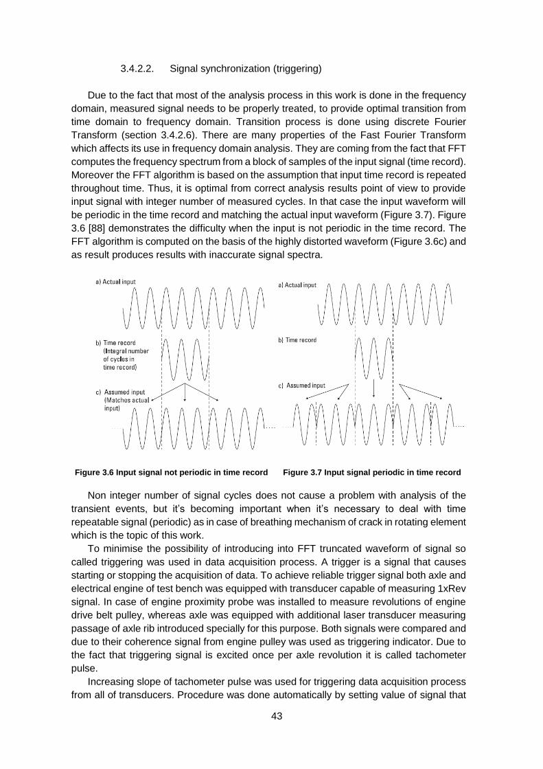
43
3.4.2.2. Signal synchronization (triggering)
Due to the fact that most of the analysis process in this work is done in the frequency
domain, measured signal needs to be properly treated, to provide optimal transition from
time domain to frequency domain. Transition process is done using discrete Fourier
Transform (section 3.4.2.6). There are many properties of the Fast Fourier Transform
which affects its use in frequency domain analysis. They are coming from the fact that FFT
computes the frequency spectrum from a block of samples of the input signal (time record).
Moreover the FFT algorithm is based on the assumption that input time record is repeated
throughout time. Thus, it is optimal from correct analysis results point of view to provide
input signal with integer number of measured cycles. In that case the input waveform will
be periodic in the time record and matching the actual input waveform (Figure 3.7). Figure
3.6 [88] demonstrates the difficulty when the input is not periodic in the time record. The
FFT algorithm is computed on the basis of the highly distorted waveform (Figure 3.6c) and
as result produces results with inaccurate signal spectra.
Figure 3.6 Input signal not periodic in time record Figure 3.7 Input signal periodic in time record
Non integer number of signal cycles does not cause a problem with analysis of the
transient events, but it’s becoming important when it’s necessary to deal with time
repeatable signal (periodic) as in case of breathing mechanism of crack in rotating element
which is the topic of this work.
To minimise the possibility of introducing into FFT truncated waveform of signal so
called triggering was used in data acquisition process. A trigger is a signal that causes
starting or stopping the acquisition of data. To achieve reliable trigger signal both axle and
electrical engine of test bench was equipped with transducer capable of measuring 1xRev
signal. In case of engine proximity probe was installed to measure revolutions of engine
drive belt pulley, whereas axle was equipped with additional laser transducer measuring
passage of axle rib introduced specially for this purpose. Both signals were compared and
due to their coherence signal from engine pulley was used as triggering indicator. Due to
the fact that triggering signal is excited once per axle revolution it is called tachometer
pulse.
Increasing slope of tachometer pulse was used for triggering data acquisition process
from all of transducers. Procedure was done automatically by setting value of signal that
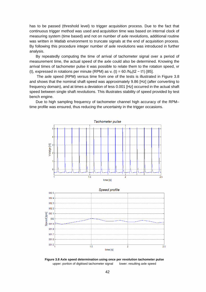
42
has to be passed (threshold level) to trigger acquisition process. Due to the fact that
continuous trigger method was used and acquisition time was based on internal clock of
measuring system (time based) and not on number of axle revolutions, additional routine
was written in Matlab environment to truncate signals at the end of acquisition process.
By following this procedure integer number of axle revolutions was introduced in further
analysis.
By repeatedly computing the time of arrival of tachometer signal over a period of
measurement time, the actual speed of the axle could also be determined. Knowing the
arrival times of tachometer pulse it was possible to relate them to the rotation speed, vr
(t), expressed in rotations per minute (RPM) as vr (t) = 60 /Np(t2 − t1) [85].
The axle speed (RPM) versus time from one of the tests is illustrated in Figure 3.8
and shows that the nominal shaft speed was approximately 9.86 [Hz] (after converting to
frequency domain), and at times a deviation of less 0.001 [Hz] occurred in the actual shaft
speed between single shaft revolutions. This illustrates stability of speed provided by test
bench engine.
Due to high sampling frequency of tachometer channel high accuracy of the RPM–
time profile was ensured, thus reducing the uncertainty in the trigger occasions.
Figure 3.8 Axle speed determination using once per revolution tachometer pulse
upper: portion of digitised tachometer signal lower: resulting axle speed
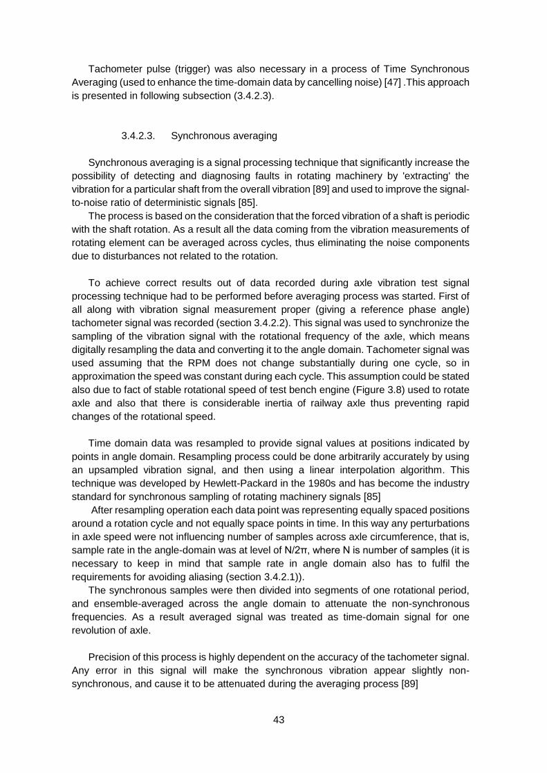
43
Tachometer pulse (trigger) was also necessary in a process of Time Synchronous
Averaging (used to enhance the time-domain data by cancelling noise) [47] .This approach
is presented in following subsection (3.4.2.3).
3.4.2.3. Synchronous averaging
Synchronous averaging is a signal processing technique that significantly increase the
possibility of detecting and diagnosing faults in rotating machinery by 'extracting' the
vibration for a particular shaft from the overall vibration [89] and used to improve the signal-
to-noise ratio of deterministic signals [85].
The process is based on the consideration that the forced vibration of a shaft is periodic
with the shaft rotation. As a result all the data coming from the vibration measurements of
rotating element can be averaged across cycles, thus eliminating the noise components
due to disturbances not related to the rotation.
To achieve correct results out of data recorded during axle vibration test signal
processing technique had to be performed before averaging process was started. First of
all along with vibration signal measurement proper (giving a reference phase angle)
tachometer signal was recorded (section 3.4.2.2). This signal was used to synchronize the
sampling of the vibration signal with the rotational frequency of the axle, which means
digitally resampling the data and converting it to the angle domain. Tachometer signal was
used assuming that the RPM does not change substantially during one cycle, so in
approximation the speed was constant during each cycle. This assumption could be stated
also due to fact of stable rotational speed of test bench engine (Figure 3.8) used to rotate
axle and also that there is considerable inertia of railway axle thus preventing rapid
changes of the rotational speed.
Time domain data was resampled to provide signal values at positions indicated by
points in angle domain. Resampling process could be done arbitrarily accurately by using
an upsampled vibration signal, and then using a linear interpolation algorithm. This
technique was developed by Hewlett-Packard in the 1980s and has become the industry
standard for synchronous sampling of rotating machinery signals [85]
After resampling operation each data point was representing equally spaced positions
around a rotation cycle and not equally space points in time. In this way any perturbations
in axle speed were not influencing number of samples across axle circumference, that is,
sample rate in the angle-domain was at level of N/2π, where N is number of samples (it is
necessary to keep in mind that sample rate in angle domain also has to fulfil the
requirements for avoiding aliasing (section 3.4.2.1)).
The synchronous samples were then divided into segments of one rotational period,
and ensemble-averaged across the angle domain to attenuate the non-synchronous
frequencies. As a result averaged signal was treated as time-domain signal for one
revolution of axle.
Precision of this process is highly dependent on the accuracy of the tachometer signal.
Any error in this signal will make the synchronous vibration appear slightly non-
synchronous, and cause it to be attenuated during the averaging process [89]
44
The scheme of synchronous averaging process applied in axle vibration analysis is
presented in Figure 3.9.
Figure 3.9 Synchronous averaging
3.4.2.4. Order analysis and windowing
When dealing with vibration analysis of rotating components it’s desirable to perform
order tracking analysis, meaning to extract information about vibration signal level in
relation with specific rotational speed of analysed component. Order in that case means
the number of occurrences of specific event in one full revolution of examined component.
As result it’s possible to obtain integer number of event occurrences (like 1x Rev, 2xRev
etc.) or in case of gearboxes or bearings non integer number of event occurrences.
Due to the fact that the spectrum of signal is not constant in length of measuring block
(due to slight deviation of rotational speed) phenomena called smearing can arise.
The smearing effect causes the peak of signal spectrum to decrease, whereas
frequency bins on both sides of the peak are increased, resulting in transferring of power
from one band to another. Leakage creates peaks at wrong frequencies, nonexisting
peaks, or change in amplitudes of existing peaks [90]. Smearing and leakage reduces the
ability to correctly observe peaks in the signal spectrum, due to creation of ‘false’ peaks
and reducing spectral resolution.
To avoid leakage phenomena so called windows are used to precondition the signal
before entering FFT process. Windows in this case are special functions by which
analysed signal is multiplicated in time domain (or convoluted in frequency domain). This
operation compress signal at the ends of window function thus allowing FFT processor to
work on non-truncated sine waves (both ends of wave entering FFT process is
compressed to zero). This operation has several implications, depending on the type of
window function used. For example very popular, general application, Hanning window
2
1
synchro
nous
avera
gin
g
synchro
nous
sam
plin
g
tachometer vibration
synchronous average
of axle vibration signal
𝟏
𝑵∑
N
45
gives very good frequency resolution but relatively poor amplitude accuracy, flat-top
window gives poor frequency resolution but highly accurate amplitude values, etc. Usage
of window functions is not intuitive, requires experience and frequently rise necessity of
trial and error approach to choose window allowing best analysis results.
In order to avoid the leakage effects discussed above, different approach was used,
namely synchronous sampling was applied instead of sampling the data with fixed
sampling frequency. According to principles of discrete Fourier Transform each frequency
line corresponds to sine wave with specific periods in the time window. This implicates
that correct measurement of desired order requires sampling synchronously sampled
signal in matter to ensure proper order resolution. Its also necessary to ensure that highest
order which is about to be measured is below 𝑁/2 frequency line (where 𝑁 is the number
of samples). To estimate required number of samples following equation can be used [85]
𝑁 = 2𝑂𝑚𝑎𝑥𝑛𝑜, where 𝑂𝑚𝑎𝑥 is the highest order under consideration, and 𝑛𝑜 is the order
resolution.
Conversion from time based sampling to angle based sampling was done using
resampling method with interpolation as described in section 3.4.2.3.
According to [85] if the resampling was perfect no time window should be necessary prior
to computing the FFT. However a flattop window was used to get the accurate amplitude
level accuracy, in case the resampling process has failed at some instance.
3.4.2.5. Initial vibration level extraction
During analysis process attempt to remove axle initial vibration signal generated by
axle shape imperfections was performed. At first laser transducer signal recorded from
one full revolution of axle rotating at slow speed was recorded. This signal was stored as
reference value for base level vibration removing process. In next steps, signal from
measurements of axle vibrations coming from normal operating speeds was segmented
based on tachometer pulse and resampled to obtain the same samples in same positions
as reference signal. Then reference signal was subtracted from remaining samples, which
after this process were reassembled back in full length signal. In next step FFT analysis
was done to investigate possible increase of vibrations caused only by the breathing
mechanism of propagating crack. After performing analysis of signals before base
vibration level extraction and after this process, this approach was dropped. Reason for
this was coming from the fact that more errors due to post processing could be introduced
in analysis process, mostly due to fact of possible thermal expansion of axle and slight
movement inside side bearer seats, thus bringing possibility of measuring different
imperfection of axle surface and introducing high errors during reference vibration signal
extraction.
3.4.2.6. Fast Fourier Transform (FFT)
Signals coming from transducers used in experiment are measurements of complex
vibration waveform. This complex waveform is a summation of all the vibrations present
at measurement location. The time waveform can be converted to a frequency spectrum
in order to indicate from where the vibration energy is coming from, by representing its
original components on a frequency versus amplitude diagram.
This is known as a vibration spectrum and is extremely valuable for fault diagnosis,
thus frequency analysis is the essence of vibration analysis and enables the satisfactory
resolution of most machine problems [88].
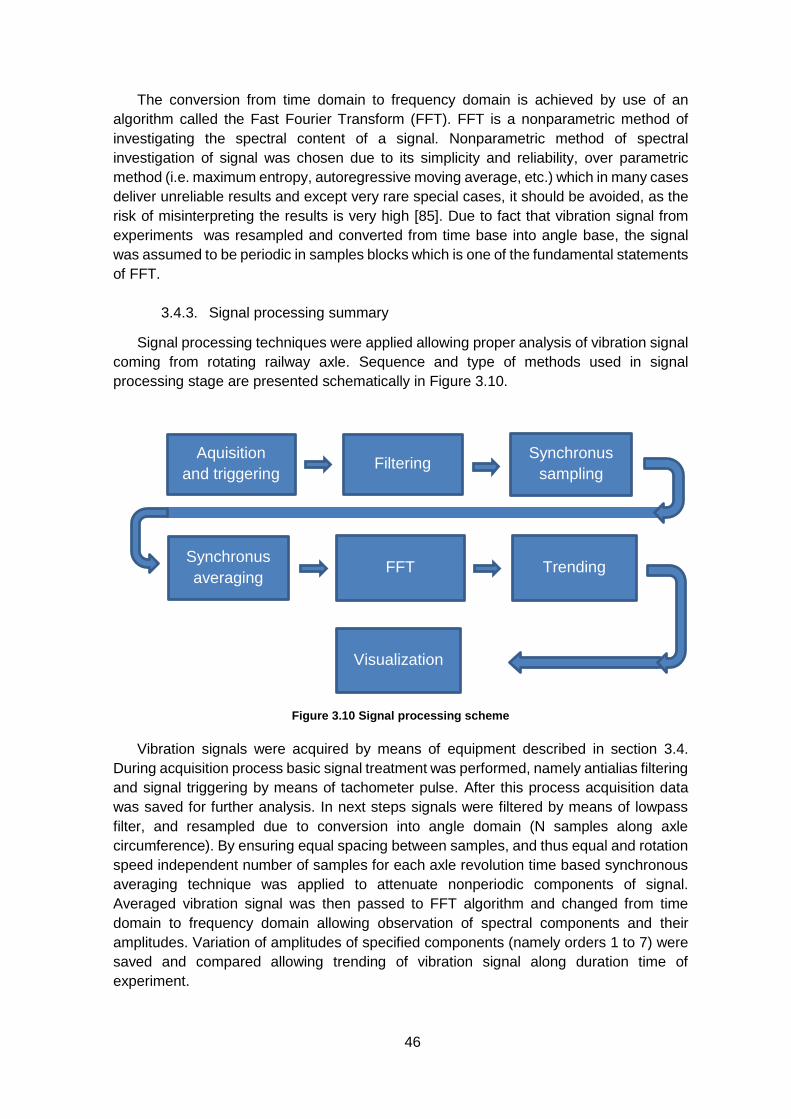
46
The conversion from time domain to frequency domain is achieved by use of an
algorithm called the Fast Fourier Transform (FFT). FFT is a nonparametric method of
investigating the spectral content of a signal. Nonparametric method of spectral
investigation of signal was chosen due to its simplicity and reliability, over parametric
method (i.e. maximum entropy, autoregressive moving average, etc.) which in many cases
deliver unreliable results and except very rare special cases, it should be avoided, as the
risk of misinterpreting the results is very high [85]. Due to fact that vibration signal from
experiments was resampled and converted from time base into angle base, the signal
was assumed to be periodic in samples blocks which is one of the fundamental statements
of FFT.
3.4.3. Signal processing summary
Signal processing techniques were applied allowing proper analysis of vibration signal
coming from rotating railway axle. Sequence and type of methods used in signal
processing stage are presented schematically in Figure 3.10.
Vibration signals were acquired by means of equipment described in section 3.4.
During acquisition process basic signal treatment was performed, namely antialias filtering
and signal triggering by means of tachometer pulse. After this process acquisition data
was saved for further analysis. In next steps signals were filtered by means of lowpass
filter, and resampled due to conversion into angle domain (N samples along axle
circumference). By ensuring equal spacing between samples, and thus equal and rotation
speed independent number of samples for each axle revolution time based synchronous
averaging technique was applied to attenuate nonperiodic components of signal.
Averaged vibration signal was then passed to FFT algorithm and changed from time
domain to frequency domain allowing observation of spectral components and their
amplitudes. Variation of amplitudes of specified components (namely orders 1 to 7) were
saved and compared allowing trending of vibration signal along duration time of
experiment.
Figure 3.10 Signal processing scheme
Aquisition
and triggering Filtering
Synchronus
sampling
Synchronus
averaging FFT Trending
Visualization
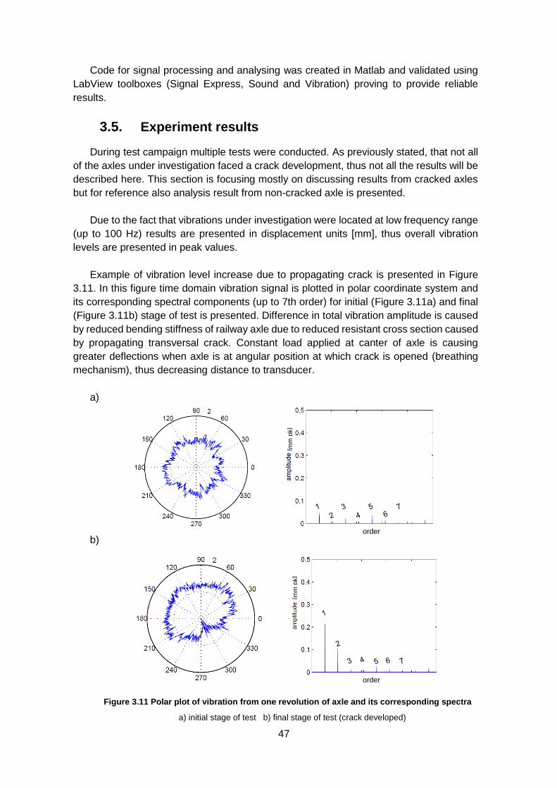
47
order
[mm
pk]
order
[mm
pk]
Code for signal processing and analysing was created in Matlab and validated using
LabView toolboxes (Signal Express, Sound and Vibration) proving to provide reliable
results.
3.5. Experiment results
During test campaign multiple tests were conducted. As previously stated, that not all
of the axles under investigation faced a crack development, thus not all the results will be
described here. This section is focusing mostly on discussing results from cracked axles
but for reference also analysis result from non-cracked axle is presented.
Due to the fact that vibrations under investigation were located at low frequency range
(up to 100 Hz) results are presented in displacement units [mm], thus overall vibration
levels are presented in peak values.
Example of vibration level increase due to propagating crack is presented in Figure
3.11. In this figure time domain vibration signal is plotted in polar coordinate system and
its corresponding spectral components (up to 7th order) for initial (Figure 3.11a) and final
(Figure 3.11b) stage of test is presented. Difference in total vibration amplitude is caused
by reduced bending stiffness of railway axle due to reduced resistant cross section caused
by propagating transversal crack. Constant load applied at canter of axle is causing
greater deflections when axle is at angular position at which crack is opened (breathing
mechanism), thus decreasing distance to transducer.
a)
b)
a) initial stage of test b) final stage of test (crack developed)
Figure 3.11 Polar plot of vibration from one revolution of axle and its corresponding spectra
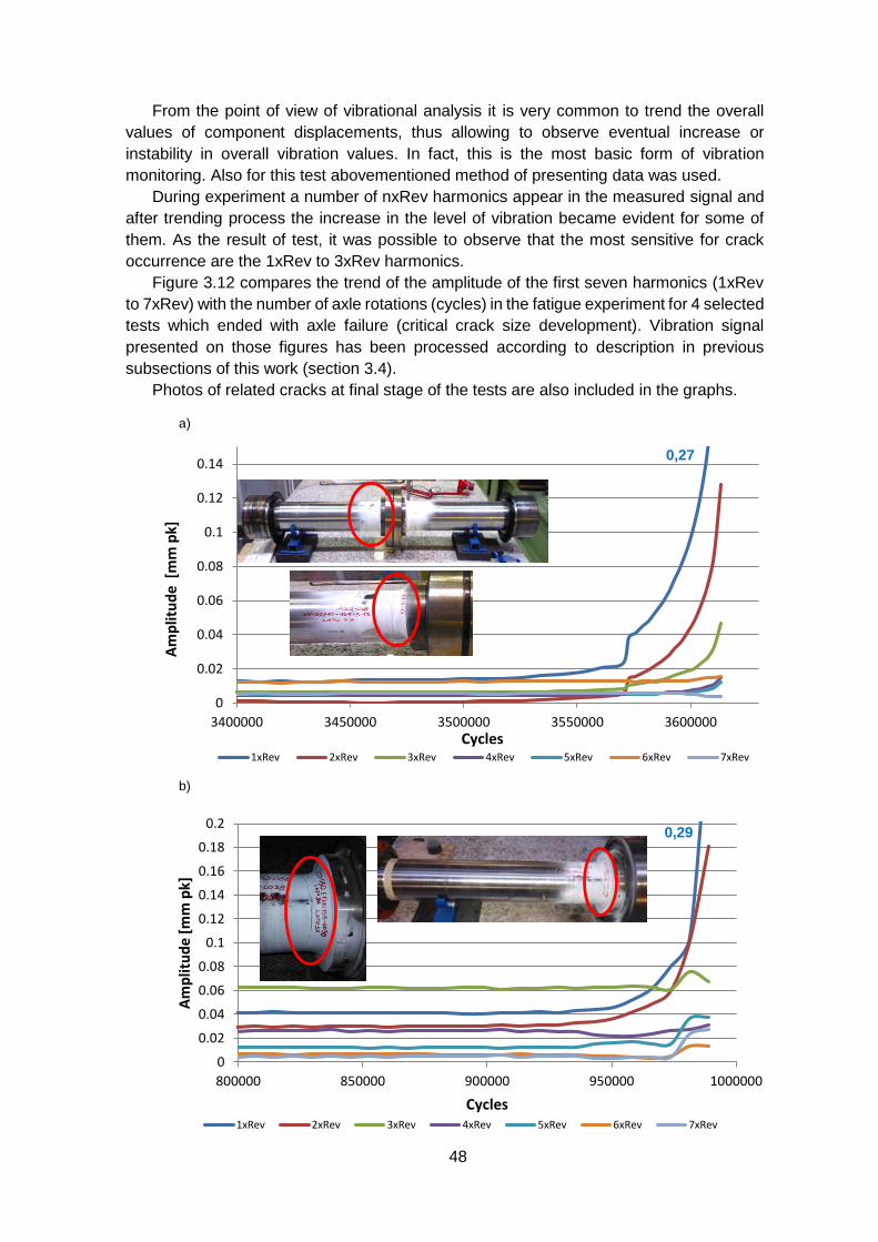
48
From the point of view of vibrational analysis it is very common to trend the overall
values of component displacements, thus allowing to observe eventual increase or
instability in overall vibration values. In fact, this is the most basic form of vibration
monitoring. Also for this test abovementioned method of presenting data was used.
During experiment a number of nxRev harmonics appear in the measured signal and
after trending process the increase in the level of vibration became evident for some of
them. As the result of test, it was possible to observe that the most sensitive for crack
occurrence are the 1xRev to 3xRev harmonics.
Figure 3.12 compares the trend of the amplitude of the first seven harmonics (1xRev
to 7xRev) with the number of axle rotations (cycles) in the fatigue experiment for 4 selected
tests which ended with axle failure (critical crack size development). Vibration signal
presented on those figures has been processed according to description in previous
subsections of this work (section 3.4).
Photos of related cracks at final stage of the tests are also included in the graphs.
a)
b)
0
0.02
0.04
0.06
0.08
0.1
0.12
0.14
3400000 3450000 3500000 3550000 3600000
Am
plit
ud
e [
mm
pk]
Cycles1xRev 2xRev 3xRev 4xRev 5xRev 6xRev 7xRev
0
0.02
0.04
0.06
0.08
0.1
0.12
0.14
0.16
0.18
0.2
800000 850000 900000 950000 1000000
Am
plit
ud
e [m
m p
k]
Cycles1xRev 2xRev 3xRev 4xRev 5xRev 6xRev 7xRev
0,27
0,29
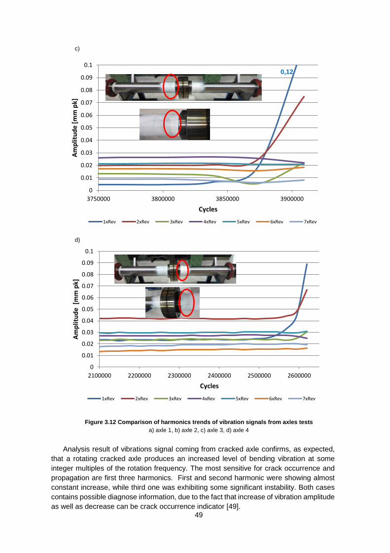
49
c)
d)
Figure 3.12 Comparison of harmonics trends of vibration signals from axles tests
a) axle 1, b) axle 2, c) axle 3, d) axle 4
Analysis result of vibrations signal coming from cracked axle confirms, as expected,
that a rotating cracked axle produces an increased level of bending vibration at some
integer multiples of the rotation frequency. The most sensitive for crack occurrence and
propagation are first three harmonics. First and second harmonic were showing almost
constant increase, while third one was exhibiting some significant instability. Both cases
contains possible diagnose information, due to the fact that increase of vibration amplitude
as well as decrease can be crack occurrence indicator [49].
0
0.01
0.02
0.03
0.04
0.05
0.06
0.07
0.08
0.09
0.1
3750000 3800000 3850000 3900000
Am
plit
ud
e [m
m p
k]
Cycles
1xRev 2xRev 3xRev 4xRev 5xRev 6xRev 7xRev
0
0.01
0.02
0.03
0.04
0.05
0.06
0.07
0.08
0.09
0.1
2100000 2200000 2300000 2400000 2500000 2600000
Am
plit
ud
e [
mm
pk]
Cycles
1xRev 2xRev 3xRev 4xRev 5xRev 6xRev 7xRev
0,12
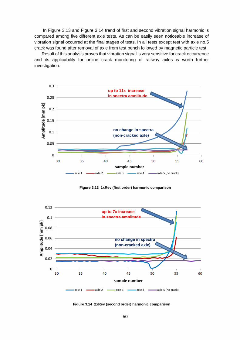
50
In Figure 3.13 and Figure 3.14 trend of first and second vibration signal harmonic is
compared among five different axle tests. As can be easily seen noticeable increase of
vibration signal occurred at the final stages of tests. In all tests except test with axle no.5
crack was found after removal of axle from test bench followed by magnetic particle test.
Result of this analysis proves that vibration signal is very sensitive for crack occurrence
and its applicability for online crack monitoring of railway axles is worth further
investigation.
Figure 3.13 1xRev (first order) harmonic comparison
Figure 3.14 2xRev (second order) harmonic comparison
0
0.05
0.1
0.15
0.2
0.25
0.3
30 35 40 45 50 55 60
Am
plit
ud
e [m
m p
k]
sample number
axle 1 axle 2 axle 3 axle 4 axle 5 (no crack)
0
0.02
0.04
0.06
0.08
0.1
0.12
25 30 35 40 45 50 55
Am
plit
ud
e [m
m p
k]
sample number
axle 1 axle 2 axle 3 axle 4 axle 5 (no crack)
up to 11x increase
in spectra amplitude
no change in spectra
(non-cracked axle)
up to 7x increase
in spectra amplitude
no change in spectra
(non-cracked axle)
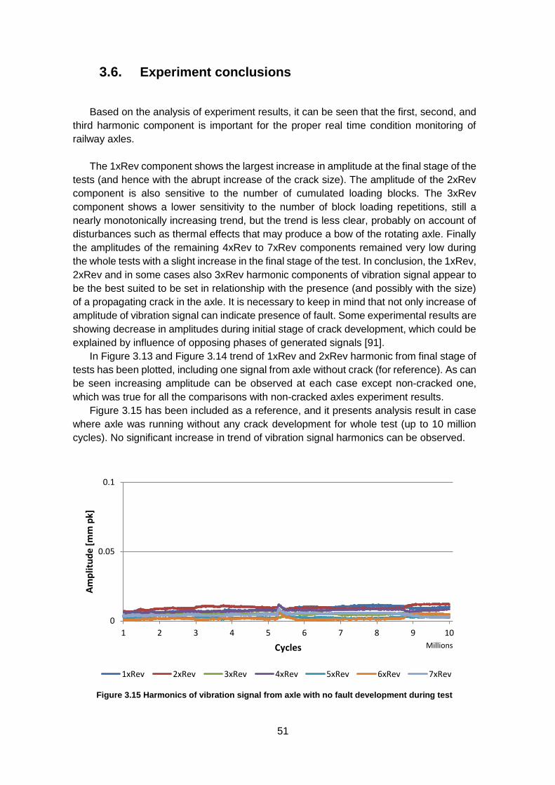
51
3.6. Experiment conclusions
Based on the analysis of experiment results, it can be seen that the first, second, and
third harmonic component is important for the proper real time condition monitoring of
railway axles.
The 1xRev component shows the largest increase in amplitude at the final stage of the
tests (and hence with the abrupt increase of the crack size). The amplitude of the 2xRev
component is also sensitive to the number of cumulated loading blocks. The 3xRev
component shows a lower sensitivity to the number of block loading repetitions, still a
nearly monotonically increasing trend, but the trend is less clear, probably on account of
disturbances such as thermal effects that may produce a bow of the rotating axle. Finally
the amplitudes of the remaining 4xRev to 7xRev components remained very low during
the whole tests with a slight increase in the final stage of the test. In conclusion, the 1xRev,
2xRev and in some cases also 3xRev harmonic components of vibration signal appear to
be the best suited to be set in relationship with the presence (and possibly with the size)
of a propagating crack in the axle. It is necessary to keep in mind that not only increase of
amplitude of vibration signal can indicate presence of fault. Some experimental results are
showing decrease in amplitudes during initial stage of crack development, which could be
explained by influence of opposing phases of generated signals [91].
In Figure 3.13 and Figure 3.14 trend of 1xRev and 2xRev harmonic from final stage of
tests has been plotted, including one signal from axle without crack (for reference). As can
be seen increasing amplitude can be observed at each case except non-cracked one,
which was true for all the comparisons with non-cracked axles experiment results.
Figure 3.15 has been included as a reference, and it presents analysis result in case
where axle was running without any crack development for whole test (up to 10 million
cycles). No significant increase in trend of vibration signal harmonics can be observed.
Figure 3.15 Harmonics of vibration signal from axle with no fault development during test
0
0.05
0.1
1 2 3 4 5 6 7 8 9 10
Am
plit
ud
e [m
m p
k]
Cycles Millions
1xRev 2xRev 3xRev 4xRev 5xRev 6xRev 7xRev
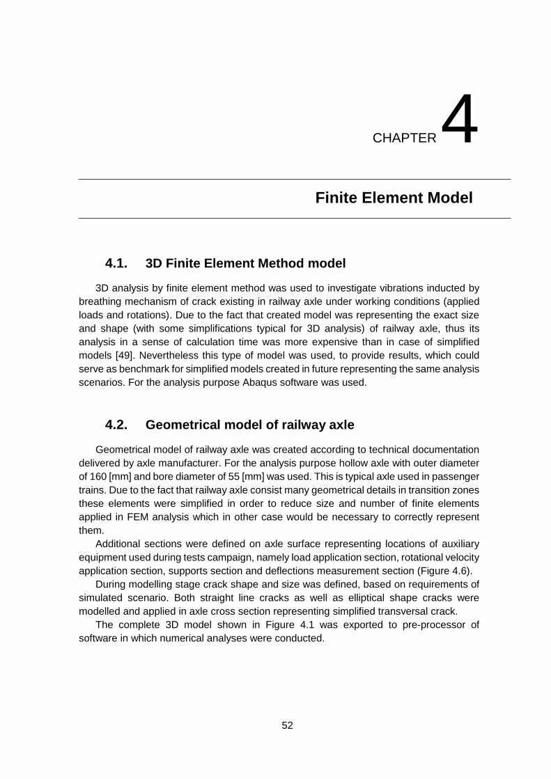
52
CHAPTER 4
4. Finite Element Model
4.1. 3D Finite Element Method model
3D analysis by finite element method was used to investigate vibrations inducted by
breathing mechanism of crack existing in railway axle under working conditions (applied
loads and rotations). Due to the fact that created model was representing the exact size
and shape (with some simplifications typical for 3D analysis) of railway axle, thus its
analysis in a sense of calculation time was more expensive than in case of simplified
models [49]. Nevertheless this type of model was used, to provide results, which could
serve as benchmark for simplified models created in future representing the same analysis
scenarios. For the analysis purpose Abaqus software was used.
4.2. Geometrical model of railway axle
Geometrical model of railway axle was created according to technical documentation
delivered by axle manufacturer. For the analysis purpose hollow axle with outer diameter
of 160 [mm] and bore diameter of 55 [mm] was used. This is typical axle used in passenger
trains. Due to the fact that railway axle consist many geometrical details in transition zones
these elements were simplified in order to reduce size and number of finite elements
applied in FEM analysis which in other case would be necessary to correctly represent
them.
Additional sections were defined on axle surface representing locations of auxiliary
equipment used during tests campaign, namely load application section, rotational velocity
application section, supports section and deflections measurement section (Figure 4.6).
During modelling stage crack shape and size was defined, based on requirements of
simulated scenario. Both straight line cracks as well as elliptical shape cracks were
modelled and applied in axle cross section representing simplified transversal crack.
The complete 3D model shown in Figure 4.1 was exported to pre-processor of
software in which numerical analyses were conducted.
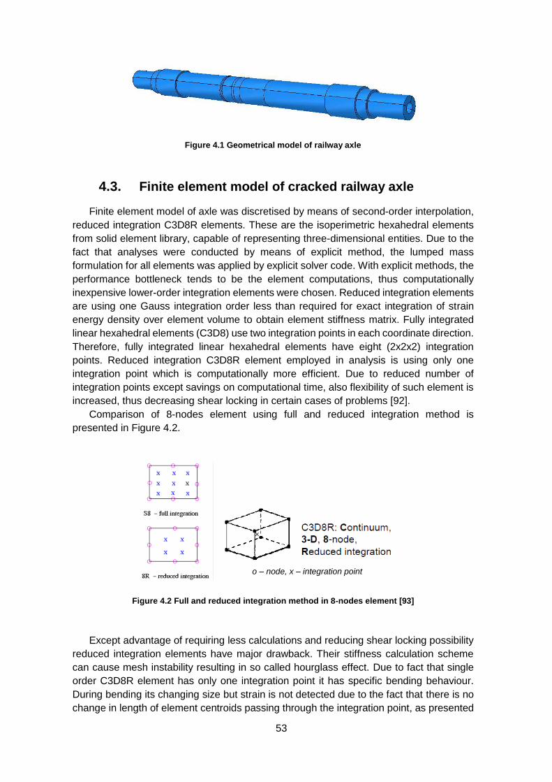
53
Figure 4.1 Geometrical model of railway axle
4.3. Finite element model of cracked railway axle
Finite element model of axle was discretised by means of second-order interpolation,
reduced integration C3D8R elements. These are the isoperimetric hexahedral elements
from solid element library, capable of representing three-dimensional entities. Due to the
fact that analyses were conducted by means of explicit method, the lumped mass
formulation for all elements was applied by explicit solver code. With explicit methods, the
performance bottleneck tends to be the element computations, thus computationally
inexpensive lower-order integration elements were chosen. Reduced integration elements
are using one Gauss integration order less than required for exact integration of strain
energy density over element volume to obtain element stiffness matrix. Fully integrated
linear hexahedral elements (C3D8) use two integration points in each coordinate direction.
Therefore, fully integrated linear hexahedral elements have eight (2x2x2) integration
points. Reduced integration C3D8R element employed in analysis is using only one
integration point which is computationally more efficient. Due to reduced number of
integration points except savings on computational time, also flexibility of such element is
increased, thus decreasing shear locking in certain cases of problems [92].
Comparison of 8-nodes element using full and reduced integration method is
presented in Figure 4.2.
Figure 4.2 Full and reduced integration method in 8-nodes element [93]
Except advantage of requiring less calculations and reducing shear locking possibility
reduced integration elements have major drawback. Their stiffness calculation scheme
can cause mesh instability resulting in so called hourglass effect. Due to fact that single
order C3D8R element has only one integration point it has specific bending behaviour.
During bending its changing size but strain is not detected due to the fact that there is no
change in length of element centroids passing through the integration point, as presented
o – node, x – integration point
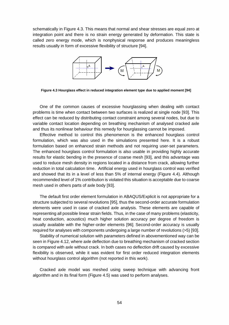
54
schematically in Figure 4.3. This means that normal and shear stresses are equal zero at
integration point and there is no strain energy generated by deformation. This state is
called zero energy mode, which is nonphysical response and produces meaningless
results usually in form of excessive flexibility of structure [94].
Figure 4.3 Hourglass effect in reduced integration element type due to applied moment [94]
One of the common causes of excessive hourglassing when dealing with contact
problems is time when contact between two surfaces is realized at single node [93]. This
effect can be reduced by distributing contact constraint among several nodes, but due to
variable contact location depending on breathing mechanism of analysed cracked axle
and thus its nonlinear behaviour this remedy for hourglassing cannot be imposed.
Effective method to control this phenomenon is the enhanced hourglass control
formulation, which was also used in the simulations presented here. It is a robust
formulation based on enhanced strain methods and not requiring user-set parameters.
The enhanced hourglass control formulation is also usable in providing highly accurate
results for elastic bending in the presence of coarse mesh [93], and this advantage was
used to reduce mesh density in regions located in a distance from crack, allowing further
reduction in total calculation time. Artificial energy used in hourglass control was verified
and showed that its in a level of less than 5% of internal energy (Figure 4.4). Although
recommended level of 1% contribution is violated this situation is acceptable due to coarse
mesh used in others parts of axle body [93].
The default first order element formulation in ABAQUS/Explicit is not appropriate for a
structure subjected to several revolutions [95], thus the second-order accurate formulation
elements were used in case of cracked axle analysis. These elements are capable of
representing all possible linear strain fields. Thus, in the case of many problems (elasticity,
heat conduction, acoustics) much higher solution accuracy per degree of freedom is
usually available with the higher-order elements [96]. Second-order accuracy is usually
required for analyses with components undergoing a large number of revolutions (>5) [93].
Stability of numerical solution with parameters defined in abovementioned way can be
seen in Figure 4.12, where axle deflection due to breathing mechanism of cracked section
is compared with axle without crack. In both cases no deflection drift caused by excessive
flexibility is observed, while it was evident for first order reduced integration elements
without hourglass control algorithm (not reported in this work).
Cracked axle model was meshed using sweep technique with advancing front
algorithm and in its final form (Figure 4.5) was used to perform analyses.
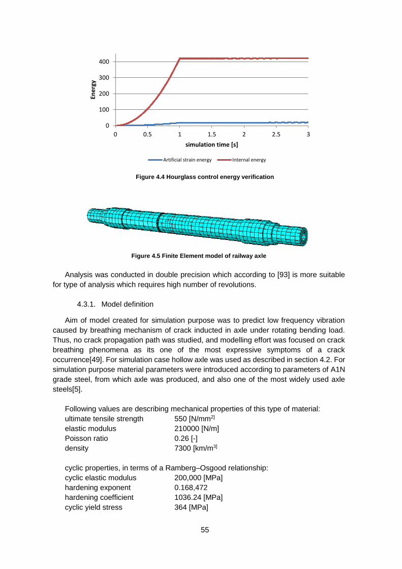
55
Figure 4.4 Hourglass control energy verification
Figure 4.5 Finite Element model of railway axle
Analysis was conducted in double precision which according to [93] is more suitable
for type of analysis which requires high number of revolutions.
4.3.1. Model definition
Aim of model created for simulation purpose was to predict low frequency vibration
caused by breathing mechanism of crack inducted in axle under rotating bending load.
Thus, no crack propagation path was studied, and modelling effort was focused on crack
breathing phenomena as its one of the most expressive symptoms of a crack
occurrence[49]. For simulation case hollow axle was used as described in section 4.2. For
simulation purpose material parameters were introduced according to parameters of A1N
grade steel, from which axle was produced, and also one of the most widely used axle
steels[5].
Following values are describing mechanical properties of this type of material:
ultimate tensile strength 550 [N/mm2]
elastic modulus 210000 [N/m]
Poisson ratio 0.26 [-]
density 7300 [km/m3]
cyclic properties, in terms of a Ramberg–Osgood relationship:
cyclic elastic modulus 200,000 [MPa]
hardening exponent 0.168,472
hardening coefficient 1036.24 [MPa]
cyclic yield stress 364 [MPa]
0
100
200
300
400
0 0.5 1 1.5 2 2.5 3
Ene
rgy
simulation time [s]
Artificial strain energy Internal energy
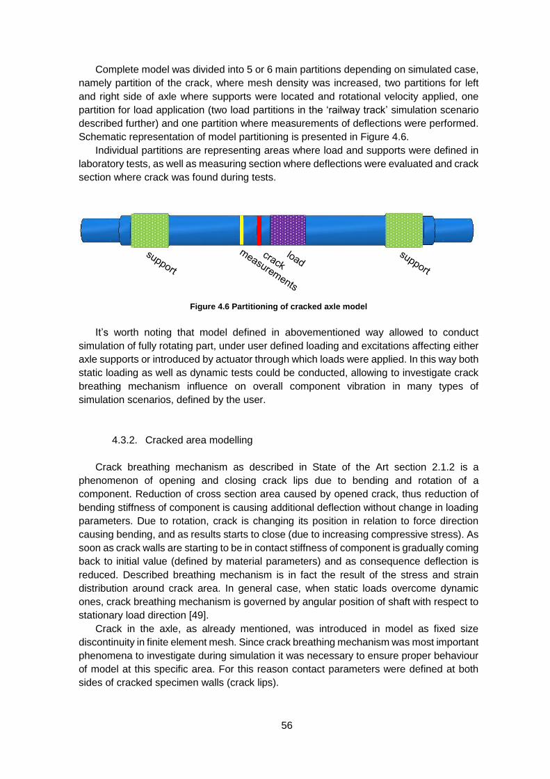
56
Complete model was divided into 5 or 6 main partitions depending on simulated case,
namely partition of the crack, where mesh density was increased, two partitions for left
and right side of axle where supports were located and rotational velocity applied, one
partition for load application (two load partitions in the ‘railway track’ simulation scenario
described further) and one partition where measurements of deflections were performed.
Schematic representation of model partitioning is presented in Figure 4.6.
Individual partitions are representing areas where load and supports were defined in
laboratory tests, as well as measuring section where deflections were evaluated and crack
section where crack was found during tests.
Figure 4.6 Partitioning of cracked axle model
It’s worth noting that model defined in abovementioned way allowed to conduct
simulation of fully rotating part, under user defined loading and excitations affecting either
axle supports or introduced by actuator through which loads were applied. In this way both
static loading as well as dynamic tests could be conducted, allowing to investigate crack
breathing mechanism influence on overall component vibration in many types of
simulation scenarios, defined by the user.
4.3.2. Cracked area modelling
Crack breathing mechanism as described in State of the Art section 2.1.2 is a
phenomenon of opening and closing crack lips due to bending and rotation of a
component. Reduction of cross section area caused by opened crack, thus reduction of
bending stiffness of component is causing additional deflection without change in loading
parameters. Due to rotation, crack is changing its position in relation to force direction
causing bending, and as results starts to close (due to increasing compressive stress). As
soon as crack walls are starting to be in contact stiffness of component is gradually coming
back to initial value (defined by material parameters) and as consequence deflection is
reduced. Described breathing mechanism is in fact the result of the stress and strain
distribution around crack area. In general case, when static loads overcome dynamic
ones, crack breathing mechanism is governed by angular position of shaft with respect to
stationary load direction [49].
Crack in the axle, as already mentioned, was introduced in model as fixed size
discontinuity in finite element mesh. Since crack breathing mechanism was most important
phenomena to investigate during simulation it was necessary to ensure proper behaviour
of model at this specific area. For this reason contact parameters were defined at both
sides of cracked specimen walls (crack lips).
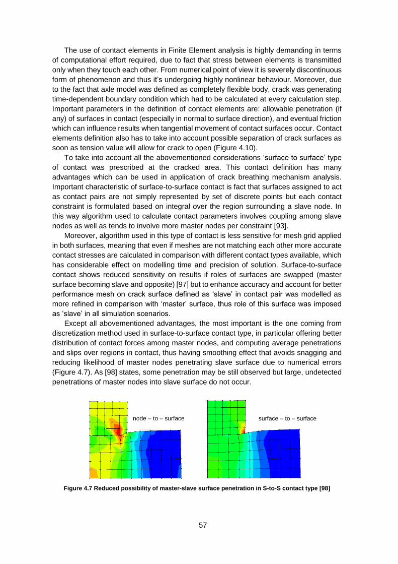
57
The use of contact elements in Finite Element analysis is highly demanding in terms
of computational effort required, due to fact that stress between elements is transmitted
only when they touch each other. From numerical point of view it is severely discontinuous
form of phenomenon and thus it’s undergoing highly nonlinear behaviour. Moreover, due
to the fact that axle model was defined as completely flexible body, crack was generating
time-dependent boundary condition which had to be calculated at every calculation step.
Important parameters in the definition of contact elements are: allowable penetration (if
any) of surfaces in contact (especially in normal to surface direction), and eventual friction
which can influence results when tangential movement of contact surfaces occur. Contact
elements definition also has to take into account possible separation of crack surfaces as
soon as tension value will allow for crack to open (Figure 4.10).
To take into account all the abovementioned considerations ‘surface to surface’ type
of contact was prescribed at the cracked area. This contact definition has many
advantages which can be used in application of crack breathing mechanism analysis.
Important characteristic of surface-to-surface contact is fact that surfaces assigned to act
as contact pairs are not simply represented by set of discrete points but each contact
constraint is formulated based on integral over the region surrounding a slave node. In
this way algorithm used to calculate contact parameters involves coupling among slave
nodes as well as tends to involve more master nodes per constraint [93].
Moreover, algorithm used in this type of contact is less sensitive for mesh grid applied
in both surfaces, meaning that even if meshes are not matching each other more accurate
contact stresses are calculated in comparison with different contact types available, which
has considerable effect on modelling time and precision of solution. Surface-to-surface
contact shows reduced sensitivity on results if roles of surfaces are swapped (master
surface becoming slave and opposite) [97] but to enhance accuracy and account for better
performance mesh on crack surface defined as ‘slave’ in contact pair was modelled as
more refined in comparison with ‘master’ surface, thus role of this surface was imposed
as ‘slave’ in all simulation scenarios.
Except all abovementioned advantages, the most important is the one coming from
discretization method used in surface-to-surface contact type, in particular offering better
distribution of contact forces among master nodes, and computing average penetrations
and slips over regions in contact, thus having smoothing effect that avoids snagging and
reducing likelihood of master nodes penetrating slave surface due to numerical errors
(Figure 4.7). As [98] states, some penetration may be still observed but large, undetected
penetrations of master nodes into slave surface do not occur.
Figure 4.7 Reduced possibility of master-slave surface penetration in S-to-S contact type [98]
surface – to – surface
node – to – surface
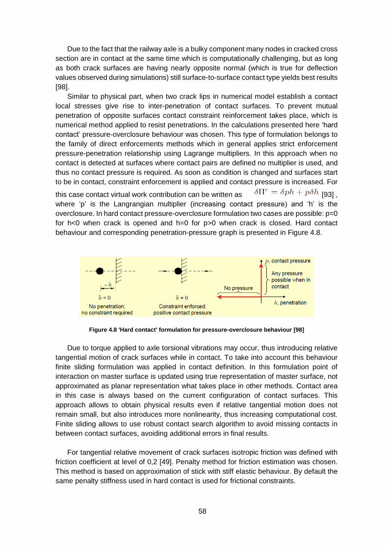
58
Due to the fact that the railway axle is a bulky component many nodes in cracked cross
section are in contact at the same time which is computationally challenging, but as long
as both crack surfaces are having nearly opposite normal (which is true for deflection
values observed during simulations) still surface-to-surface contact type yields best results
[98].
Similar to physical part, when two crack lips in numerical model establish a contact
local stresses give rise to inter-penetration of contact surfaces. To prevent mutual
penetration of opposite surfaces contact constraint reinforcement takes place, which is
numerical method applied to resist penetrations. In the calculations presented here ‘hard
contact’ pressure-overclosure behaviour was chosen. This type of formulation belongs to
the family of direct enforcements methods which in general applies strict enforcement
pressure-penetration relationship using Lagrange multipliers. In this approach when no
contact is detected at surfaces where contact pairs are defined no multiplier is used, and
thus no contact pressure is required. As soon as condition is changed and surfaces start
to be in contact, constraint enforcement is applied and contact pressure is increased. For
this case contact virtual work contribution can be written as [93] ,
where ‘p’ is the Langrangian multiplier (increasing contact pressure) and ‘h’ is the
overclosure. In hard contact pressure-overclosure formulation two cases are possible: p=0
for h<0 when crack is opened and h=0 for p>0 when crack is closed. Hard contact
behaviour and corresponding penetration-pressure graph is presented in Figure 4.8.
Figure 4.8 'Hard contact' formulation for pressure-overclosure behaviour [98]
Due to torque applied to axle torsional vibrations may occur, thus introducing relative
tangential motion of crack surfaces while in contact. To take into account this behaviour
finite sliding formulation was applied in contact definition. In this formulation point of
interaction on master surface is updated using true representation of master surface, not
approximated as planar representation what takes place in other methods. Contact area
in this case is always based on the current configuration of contact surfaces. This
approach allows to obtain physical results even if relative tangential motion does not
remain small, but also introduces more nonlinearity, thus increasing computational cost.
Finite sliding allows to use robust contact search algorithm to avoid missing contacts in
between contact surfaces, avoiding additional errors in final results.
For tangential relative movement of crack surfaces isotropic friction was defined with
friction coefficient at level of 0,2 [49]. Penalty method for friction estimation was chosen.
This method is based on approximation of stick with stiff elastic behaviour. By default the
same penalty stiffness used in hard contact is used for frictional constraints.
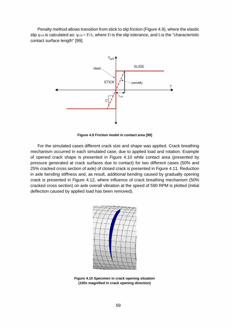
59
Penalty method allows transition from stick to slip friction (Figure 4.9), where the elastic
slip γcrit is calculated as: γcrit = Ff li, where Ff is the slip tolerance, and li is the "characteristic
contact surface length" [99].
Figure 4.9 Friction model in contact area [99]
For the simulated cases different crack size and shape was applied. Crack breathing
mechanism occurred in each simulated case, due to applied load and rotation. Example
of opened crack shape is presented in Figure 4.10 while contact area (presented by
pressure generated at crack surfaces due to contact) for two different cases (50% and
25% cracked cross section of axle) of closed crack is presented in Figure 4.11. Reduction
in axle bending stiffness and, as result, additional bending caused by gradually opening
crack is presented in Figure 4.12, where influence of crack breathing mechanism (50%
cracked cross section) on axle overall vibration at the speed of 590 RPM is plotted (initial
deflection caused by applied load has been removed).
Figure 4.10 Specimen in crack opening situation
(100x magnified in crack opening direction)
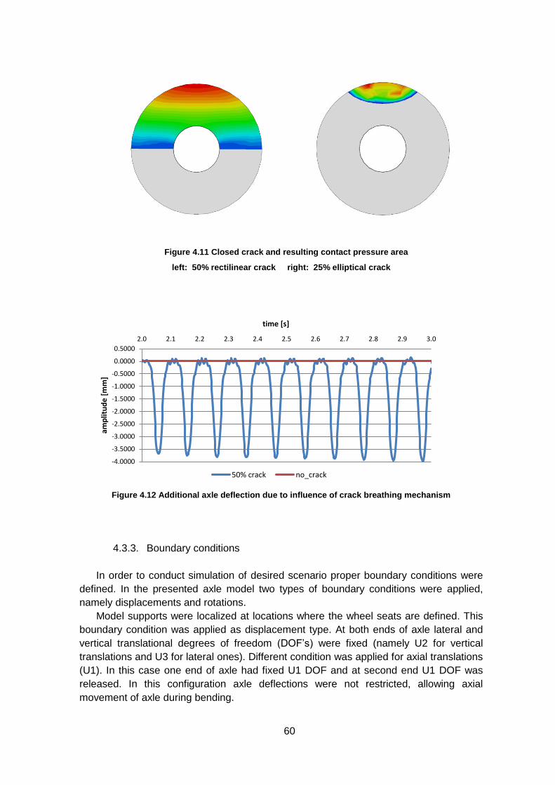
60
left: 50% rectilinear crack right: 25% elliptical crack
Figure 4.12 Additional axle deflection due to influence of crack breathing mechanism
4.3.3. Boundary conditions
In order to conduct simulation of desired scenario proper boundary conditions were
defined. In the presented axle model two types of boundary conditions were applied,
namely displacements and rotations.
Model supports were localized at locations where the wheel seats are defined. This
boundary condition was applied as displacement type. At both ends of axle lateral and
vertical translational degrees of freedom (DOF’s) were fixed (namely U2 for vertical
translations and U3 for lateral ones). Different condition was applied for axial translations
(U1). In this case one end of axle had fixed U1 DOF and at second end U1 DOF was
released. In this configuration axle deflections were not restricted, allowing axial
movement of axle during bending.
-4.0000
-3.5000
-3.0000
-2.5000
-2.0000
-1.5000
-1.0000
-0.5000
0.0000
0.5000
2.0 2.1 2.2 2.3 2.4 2.5 2.6 2.7 2.8 2.9 3.0
amp
litu
de
[m
m]
time [s]
50% crack no_crack
Figure 4.11 Closed crack and resulting contact pressure area
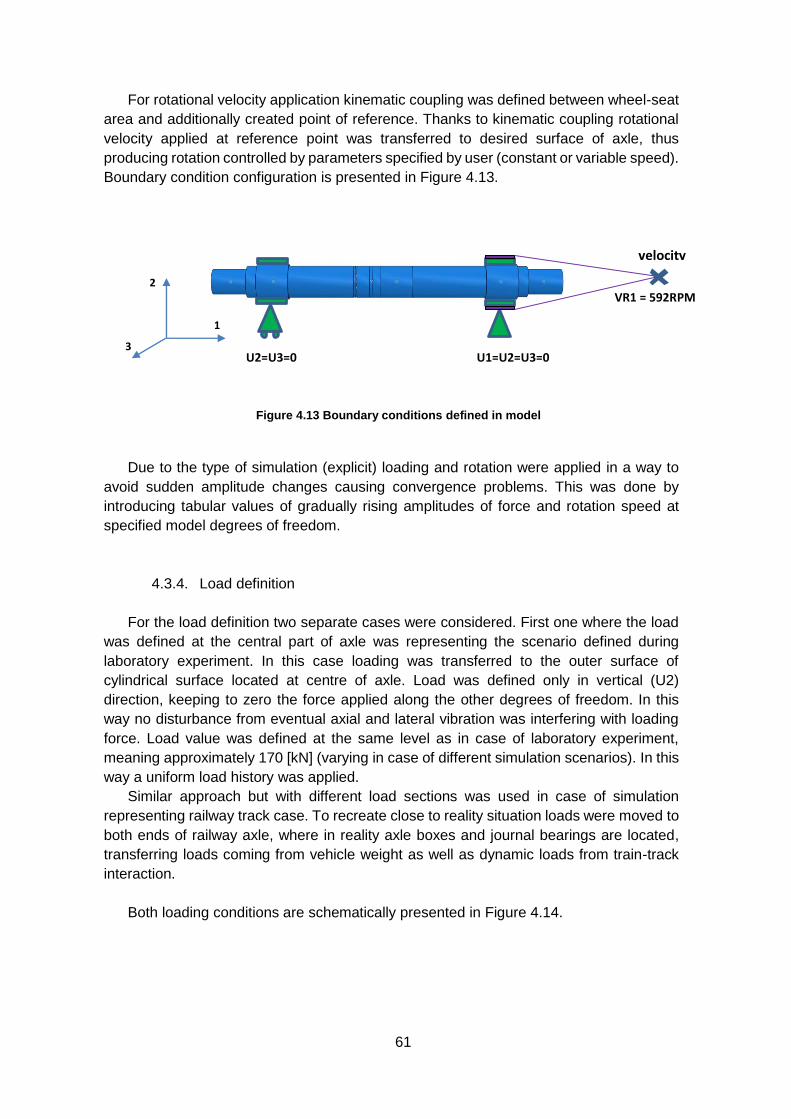
61
For rotational velocity application kinematic coupling was defined between wheel-seat
area and additionally created point of reference. Thanks to kinematic coupling rotational
velocity applied at reference point was transferred to desired surface of axle, thus
producing rotation controlled by parameters specified by user (constant or variable speed).
Boundary condition configuration is presented in Figure 4.13.
Due to the type of simulation (explicit) loading and rotation were applied in a way to
avoid sudden amplitude changes causing convergence problems. This was done by
introducing tabular values of gradually rising amplitudes of force and rotation speed at
specified model degrees of freedom.
4.3.4. Load definition
For the load definition two separate cases were considered. First one where the load
was defined at the central part of axle was representing the scenario defined during
laboratory experiment. In this case loading was transferred to the outer surface of
cylindrical surface located at centre of axle. Load was defined only in vertical (U2)
direction, keeping to zero the force applied along the other degrees of freedom. In this
way no disturbance from eventual axial and lateral vibration was interfering with loading
force. Load value was defined at the same level as in case of laboratory experiment,
meaning approximately 170 [kN] (varying in case of different simulation scenarios). In this
way a uniform load history was applied.
Similar approach but with different load sections was used in case of simulation
representing railway track case. To recreate close to reality situation loads were moved to
both ends of railway axle, where in reality axle boxes and journal bearings are located,
transferring loads coming from vehicle weight as well as dynamic loads from train-track
interaction.
Both loading conditions are schematically presented in Figure 4.14.
velocity
U1=U2=U3=0 U2=U3=0
VR1 = 592RPM 2
3
1
Figure 4.13 Boundary conditions defined in model
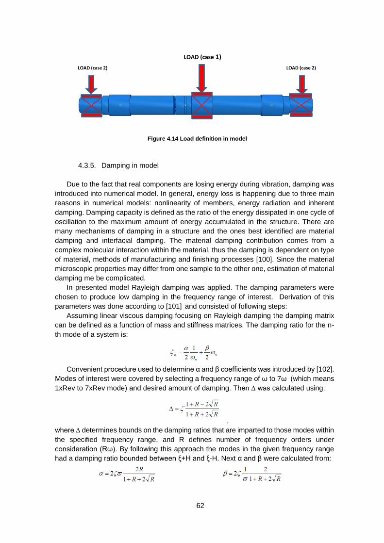
62
4.3.5. Damping in model
Due to the fact that real components are losing energy during vibration, damping was
introduced into numerical model. In general, energy loss is happening due to three main
reasons in numerical models: nonlinearity of members, energy radiation and inherent
damping. Damping capacity is defined as the ratio of the energy dissipated in one cycle of
oscillation to the maximum amount of energy accumulated in the structure. There are
many mechanisms of damping in a structure and the ones best identified are material
damping and interfacial damping. The material damping contribution comes from a
complex molecular interaction within the material, thus the damping is dependent on type
of material, methods of manufacturing and finishing processes [100]. Since the material
microscopic properties may differ from one sample to the other one, estimation of material
damping me be complicated.
In presented model Rayleigh damping was applied. The damping parameters were
chosen to produce low damping in the frequency range of interest. Derivation of this
parameters was done according to [101] and consisted of following steps:
Assuming linear viscous damping focusing on Rayleigh damping the damping matrix
can be defined as a function of mass and stiffness matrices. The damping ratio for the n-
th mode of a system is:
Convenient procedure used to determine α and β coefficients was introduced by [102].
Modes of interest were covered by selecting a frequency range of ω to 7ω (which means
1xRev to 7xRev mode) and desired amount of damping. Then ∆ was calculated using:
,
where ∆ determines bounds on the damping ratios that are imparted to those modes within
the specified frequency range, and R defines number of frequency orders under
consideration (Rω). By following this approach the modes in the given frequency range
had a damping ratio bounded between ξ+H and ξ-H. Next α and β were calculated from:
LOAD (case 1)
LOAD (case 2) LOAD (case 2)
Figure 4.14 Load definition in model
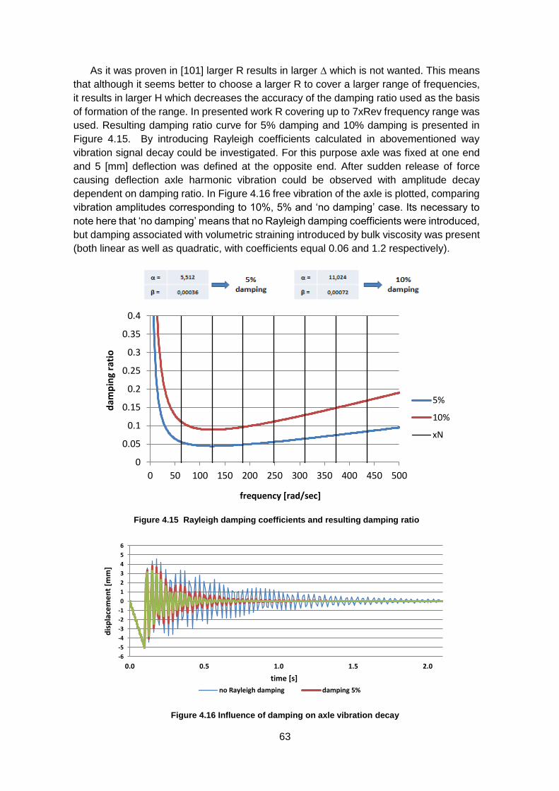
63
As it was proven in [101] larger R results in larger ∆ which is not wanted. This means
that although it seems better to choose a larger R to cover a larger range of frequencies,
it results in larger H which decreases the accuracy of the damping ratio used as the basis
of formation of the range. In presented work R covering up to 7xRev frequency range was
used. Resulting damping ratio curve for 5% damping and 10% damping is presented in
Figure 4.15. By introducing Rayleigh coefficients calculated in abovementioned way
vibration signal decay could be investigated. For this purpose axle was fixed at one end
and 5 [mm] deflection was defined at the opposite end. After sudden release of force
causing deflection axle harmonic vibration could be observed with amplitude decay
dependent on damping ratio. In Figure 4.16 free vibration of the axle is plotted, comparing
vibration amplitudes corresponding to 10%, 5% and ‘no damping’ case. Its necessary to
note here that ‘no damping’ means that no Rayleigh damping coefficients were introduced,
but damping associated with volumetric straining introduced by bulk viscosity was present
(both linear as well as quadratic, with coefficients equal 0.06 and 1.2 respectively).
Figure 4.15 Rayleigh damping coefficients and resulting damping ratio
Figure 4.16 Influence of damping on axle vibration decay
0
0.05
0.1
0.15
0.2
0.25
0.3
0.35
0.4
0 50 100 150 200 250 300 350 400 450 500
dam
pin
g ra
tio
frequency [rad/sec]
5%
10%
xN
-6
-5
-4
-3
-2
-1
0
1
2
3
4
5
6
0.0 0.5 1.0 1.5 2.0
dis
pla
cem
en
t [m
m]
time [s]
no Rayleigh damping damping 5%
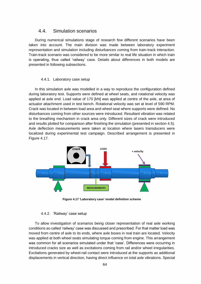
64
4.4. Simulation scenarios
During numerical simulations stage of research few different scenarios have been
taken into account. The main division was made between laboratory experiment
representation and simulation including disturbances coming from train-track interaction.
Train-track scenario was considered to be more similar to real life situation in which train
is operating, thus called ‘railway’ case. Details about differences in both models are
presented in following subsections.
4.4.1. Laboratory case setup
In this simulation axle was modelled in a way to reproduce the configuration defined
during laboratory test. Supports were defined at wheel seats, and rotational velocity was
applied at axle end. Load value of 170 [kN] was applied at centre of the axle, at area of
actuator attachment used in test bench. Rotational velocity was set at level of 590 RPM.
Crack was located in between load area and wheel seat where supports were defined. No
disturbances coming from other sources were introduced. Resultant vibration was related
to the breathing mechanism in crack area only. Different sizes of crack were introduced
and results plotted for comparison after finishing the simulation (presented in section 4.5).
Axle deflection measurements were taken at location where lasers transducers were
localized during experimental test campaign. Described arrangement is presented in
Figure 4.17.
Figure 4.17 'Laboratory case' model definition scheme
4.4.2. ‘Railway’ case setup
To allow investigation of scenarios being closer representation of real axle working
conditions so called ‘railway’ case was discussed and prescribed. For that matter load was
moved from centre of axle to its ends, where axle boxes in real train are located. Velocity
was applied at both wheel seats simulating torque coming from engine. This arrangement
was common for all scenarios simulated under that ‘case’. Differences were occurring in
introduced cracks size as well as excitations coming from rail and/or wheel irregularities.
Excitations generated by wheel-rail contact were introduced at the supports as additional
displacements in vertical direction, having direct influence on total axle vibrations. Special
crack
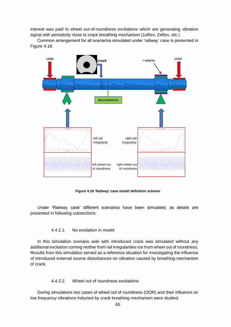
65
interest was paid to wheel out-of-roundness excitations which are generating vibration
signal with periodicity close to crack breathing mechanism (1xRev, 2xRev, etc.)
Common arrangement for all scenarios simulated under ‘railway’ case is presented in
Figure 4.18.
Figure 4.18 'Railway' case model definition scheme
Under ‘Railway case' different scenarios have been simulated, as details are
presented in following subsections.
4.4.2.1. No excitation in model
In this simulation scenario axle with introduced crack was simulated without any
additional excitation coming neither from rail irregularities nor from wheel out of roundness.
Results from this simulation served as a reference situation for investigating the influence
of introduced external source disturbances on vibration caused by breathing mechanism
of crack.
4.4.2.2. Wheel out of roundness excitations
During simulations two cases of wheel out of roundness (OOR) and their influence on
low frequency vibrations inducted by crack breathing mechanism were studied.
crack
left wheel out
of roundness
left rail
irregularity
right rail
irregularity
right wheel out
of roundness
0 0.5 1 1.5 2 2.5 3
-0.2
0
0.2
0.4
Worn Wheel irregularity profile
Time [s]
Irregula
rity [m
m]
1 2 3 4 5 6 7 8 9 10 11 12 13 14 15 16 17 18 19 200
0.05
0.1
0.15One-Sided Amplitude Spectrum of worn wheel irregularity profile
Order [-]
Fourie
r spectrum
0 0.5 1 1.5 2 2.5 3
-0.2
0
0.2
0.4
Worn Wheel irregularity profile
Time [s]
Irregula
rity [m
m]
1 2 3 4 5 6 7 8 9 10 11 12 13 14 15 16 17 18 19 200
0.05
0.1
0.15One-Sided Amplitude Spectrum of worn wheel irregularity profile
Order [-]
Fourie
r spectrum
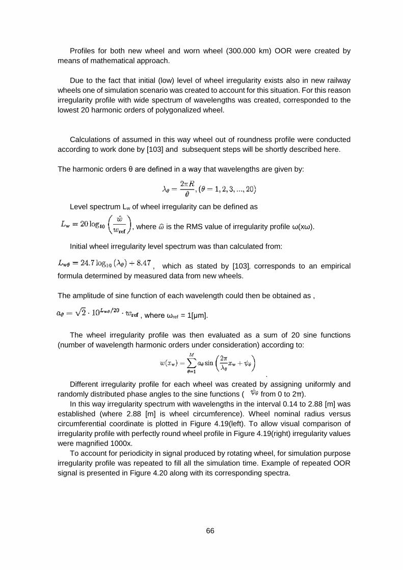
66
Profiles for both new wheel and worn wheel (300.000 km) OOR were created by
means of mathematical approach.
Due to the fact that initial (low) level of wheel irregularity exists also in new railway
wheels one of simulation scenario was created to account for this situation. For this reason
irregularity profile with wide spectrum of wavelengths was created, corresponded to the
lowest 20 harmonic orders of polygonalized wheel.
Calculations of assumed in this way wheel out of roundness profile were conducted
according to work done by [103] and subsequent steps will be shortly described here.
The harmonic orders θ are defined in a way that wavelengths are given by:
Level spectrum Lw of wheel irregularity can be defined as
, where �̂� is the RMS value of irregularity profile ω(xω).
Initial wheel irregularity level spectrum was than calculated from:
, which as stated by [103], corresponds to an empirical
formula determined by measured data from new wheels.
The amplitude of sine function of each wavelength could then be obtained as ,
, where ωref = 1[μm].
The wheel irregularity profile was then evaluated as a sum of 20 sine functions
(number of wavelength harmonic orders under consideration) according to:
.
Different irregularity profile for each wheel was created by assigning uniformly and
randomly distributed phase angles to the sine functions ( f from 0 to 2π).
In this way irregularity spectrum with wavelengths in the interval 0.14 to 2.88 [m] was
established (where 2.88 [m] is wheel circumference). Wheel nominal radius versus
circumferential coordinate is plotted in Figure 4.19(left). To allow visual comparison of
irregularity profile with perfectly round wheel profile in Figure 4.19(right) irregularity values
were magnified 1000x.
To account for periodicity in signal produced by rotating wheel, for simulation purpose
irregularity profile was repeated to fill all the simulation time. Example of repeated OOR
signal is presented in Figure 4.20 along with its corresponding spectra.
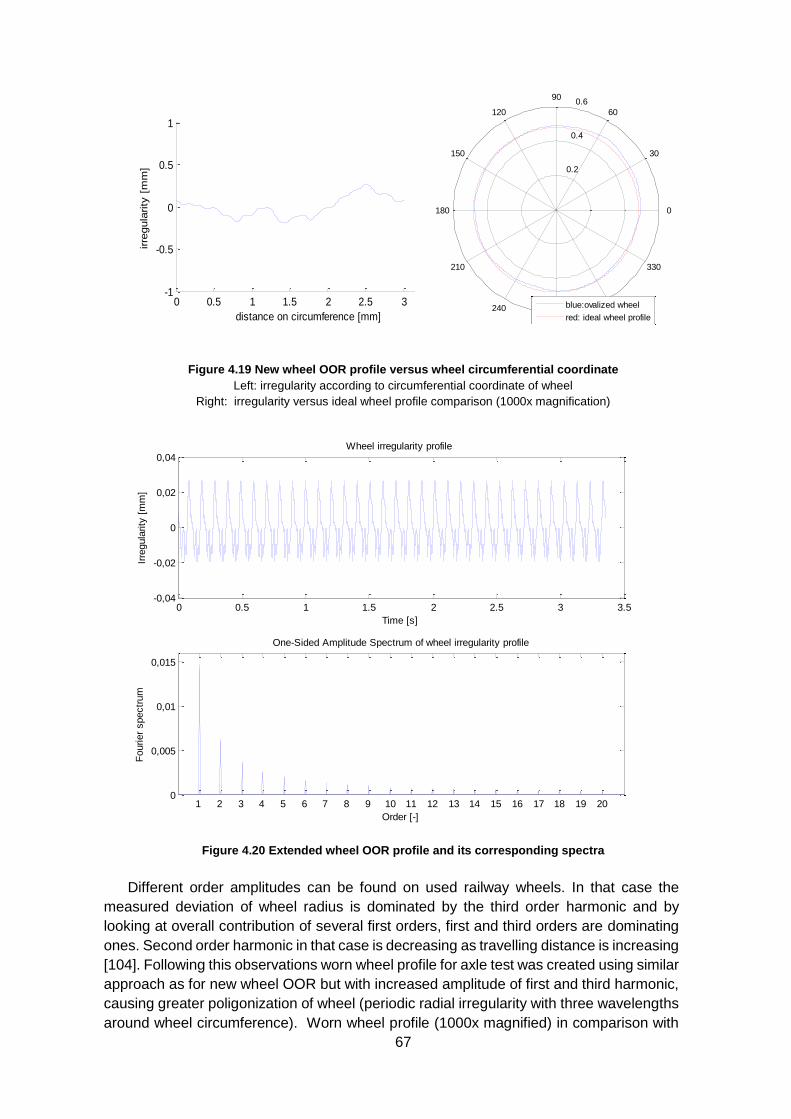
67
Figure 4.19 New wheel OOR profile versus wheel circumferential coordinate
Left: irregularity according to circumferential coordinate of wheel
Right: irregularity versus ideal wheel profile comparison (1000x magnification)
Figure 4.20 Extended wheel OOR profile and its corresponding spectra
Different order amplitudes can be found on used railway wheels. In that case the
measured deviation of wheel radius is dominated by the third order harmonic and by
looking at overall contribution of several first orders, first and third orders are dominating
ones. Second order harmonic in that case is decreasing as travelling distance is increasing
[104]. Following this observations worn wheel profile for axle test was created using similar
approach as for new wheel OOR but with increased amplitude of first and third harmonic,
causing greater poligonization of wheel (periodic radial irregularity with three wavelengths
around wheel circumference). Worn wheel profile (1000x magnified) in comparison with
0 0.5 1 1.5 2 2.5 3 3.5-1
-0.5
0
0.5
1x 10
-4 Wheel irregularity profile
distance on circumference [mm]
irre
gula
rity
[m
m] 0.2
0.4
0.6
30
210
60
240
90
270
120
300
150
330
180 0
Wheel OOR
blue:ovalized wheel
red: ideal wheel profile
0 0.5 1 1.5 2 2.5 3 3.5-0,04
-0,02
0
0,02
0,04Wheel irregularity profile
Time [s]
Irre
gula
rity
[m
m]
1 2 3 4 5 6 7 8 9 10 11 12 13 14 15 16 17 18 19 200
0,005
0,01
0,015
One-Sided Amplitude Spectrum of wheel irregularity profile
Order [-]
Fourier
spectr
um
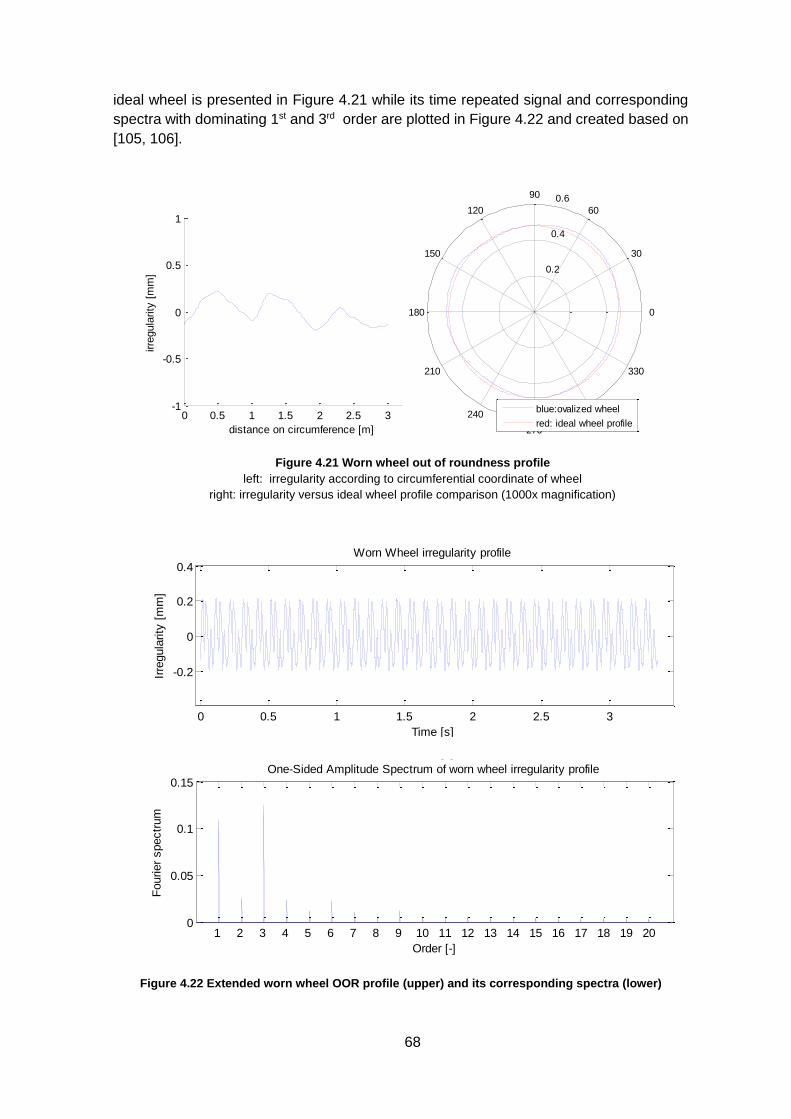
68
ideal wheel is presented in Figure 4.21 while its time repeated signal and corresponding
spectra with dominating 1st and 3rd order are plotted in Figure 4.22 and created based on
[105, 106].
Figure 4.21 Worn wheel out of roundness profile
left: irregularity according to circumferential coordinate of wheel
right: irregularity versus ideal wheel profile comparison (1000x magnification)
Figure 4.22 Extended worn wheel OOR profile (upper) and its corresponding spectra (lower)
0 0.5 1 1.5 2 2.5 3 3.5-1
-0.5
0
0.5
1Wheel irregularity profile
distance on circumference [m]
irre
gula
rity
[m
m] 0.2
0.4
0.6
30
210
60
240
90
270
120
300
150
330
180 0
Worn Wheel OOR
blue:ovalized wheel
red: ideal wheel profile
0 0.5 1 1.5 2 2.5 3
-0.2
0
0.2
0.4
Worn Wheel irregularity profile
Time [s]
Irre
gula
rity
[m
m]
1 2 3 4 5 6 7 8 9 10 11 12 13 14 15 16 17 18 19 200
0.05
0.1
0.15One-Sided Amplitude Spectrum of worn wheel irregularity profile
Order [-]
Fourier
spectr
um
0 0.5 1 1.5 2 2.5 3
-0.2
0
0.2
0.4
Worn Wheel irregularity profile
Time [s]
Irre
gula
rity
[m
m]
1 2 3 4 5 6 7 8 9 10 11 12 13 14 15 16 17 18 19 200
0.05
0.1
0.15One-Sided Amplitude Spectrum of worn wheel irregularity profile
Order [-]
Fourier
spectr
um
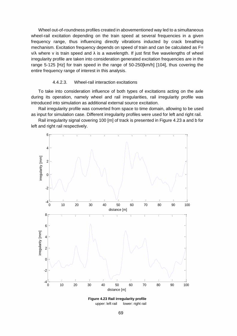
69
Wheel out-of-roundness profiles created in abovementioned way led to a simultaneous
wheel-rail excitation depending on the train speed at several frequencies in a given
frequency range, thus influencing directly vibrations inducted by crack breathing
mechanism. Excitation frequency depends on speed of train and can be calculated as F=
v/λ where v is train speed and λ is a wavelength. If just first five wavelengths of wheel
irregularity profile are taken into consideration generated excitation frequencies are in the
range 5-125 [Hz] for train speed in the range of 50-250[km/h] [104], thus covering the
entire frequency range of interest in this analysis.
4.4.2.3. Wheel-rail interaction excitations
To take into consideration influence of both types of excitations acting on the axle
during its operation, namely wheel and rail irregularities, rail irregularity profile was
introduced into simulation as additional external source excitation.
Rail irregularity profile was converted from space to time domain, allowing to be used
as input for simulation case. Different irregularity profiles were used for left and right rail.
Rail irregularity signal covering 100 [m] of track is presented in Figure 4.23 a and b for
left and right rail respectively.
Figure 4.23 Rail irregularity profile
upper: left rail lower: right rail
0 10 20 30 40 50 60 70 80 90 100-4
-2
0
2
4
6x 10
-3
distance [m]
irre
gulrity [
m]
0 10 20 30 40 50 60 70 80 90 100-4
-2
0
2
4
6
8x 10
-3
irre
gulrity [
m]
distance [m]
0 10 20 30 40 50 60 70 80 90 100-4
-2
0
2
4
6
distance [m]
irre
gula
rity
[m
m]
0 10 20 30 40 50 60 70 80 90 100-4
-2
0
2
4
6
distance [m]
irre
gula
rity
[m
m]
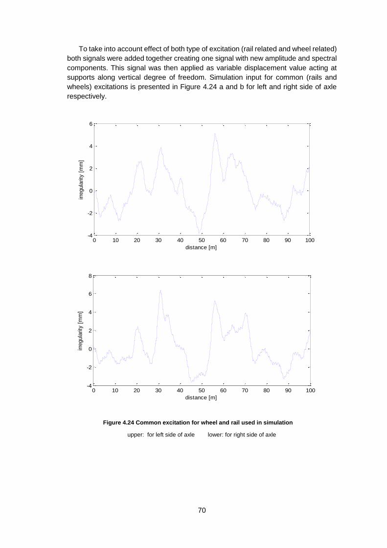
70
To take into account effect of both type of excitation (rail related and wheel related)
both signals were added together creating one signal with new amplitude and spectral
components. This signal was then applied as variable displacement value acting at
supports along vertical degree of freedom. Simulation input for common (rails and
wheels) excitations is presented in Figure 4.24 a and b for left and right side of axle
respectively.
upper: for left side of axle lower: for right side of axle
0 10 20 30 40 50 60 70 80 90 100-4
-2
0
2
4
6
distance [m]
irre
gula
rity
[m
m]
0 10 20 30 40 50 60 70 80 90 100-4
-2
0
2
4
6
8
distance [m]
irre
gula
rity
[m
m]
Figure 4.24 Common excitation for wheel and rail used in simulation
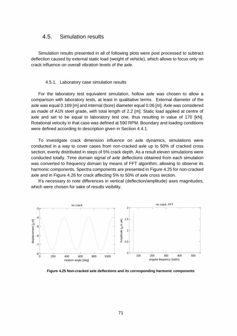
71
4.5. Simulation results
Simulation results presented in all of following plots were post processed to subtract
deflection caused by external static load (weight of vehicle), which allows to focus only on
crack influence on overall vibration levels of the axle.
4.5.1. Laboratory case simulation results
For the laboratory test equivalent simulation, hollow axle was chosen to allow a
comparison with laboratory tests, at least in qualitative terms. External diameter of the
axle was equal 0.169 [m] and internal (bore) diameter equal 0.06 [m]. Axle was considered
as made of A1N steel grade, with total length of 2.2 [m]. Static load applied at centre of
axle and set to be equal to laboratory test one, thus resulting in value of 170 [kN].
Rotational velocity in that case was defined at 590 RPM. Boundary and loading conditions
were defined according to description given in Section 4.4.1.
To investigate crack dimension influence on axle dynamics, simulations were
conducted in a way to cover cases from non-cracked axle up to 50% of cracked cross
section, evenly distributed in steps of 5% crack depth. As a result eleven simulations were
conducted totally. Time domain signal of axle deflections obtained from each simulation
was converted to frequency domain by means of FFT algorithm, allowing to observe its
harmonic components. Spectra components are presented in Figure 4.25 for non-cracked
axle and in Figure 4.26 for crack affecting 5% to 50% of axle cross section.
It’s necessary to note differences in vertical (deflection/amplitude) axes magnitudes,
which were chosen for sake of results visibility.
Figure 4.25 Non-cracked axle deflections and its corresponding harmonic components
0 200 400 600 800 1000-8
-7
-6
-5
-4
-3no crack
rotation angle [deg]
dis
pla
cem
ent
[ m
]
100 200 300 400 5000
0,5
1
1,5
2
angular frequency [rad/s]
Am
plitu
de [
m p
k]
no crack, FFT
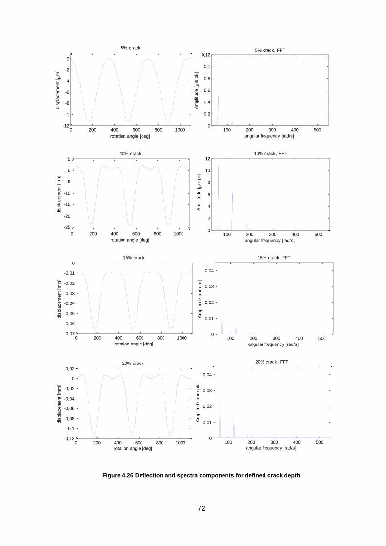
72
Figure 4.26 Deflection and spectra components for defined crack depth
0 200 400 600 800 1000-12
-1
-8
-6
-4
-2
0
5% crack
rotation angle [deg]
dis
pla
cem
ent
[ m
]
100 200 300 400 5000
0,2
0,4
0,6
0,8
0,1
0,12
angular frequency [rad/s]
Am
plit
ude [
m p
k]
5% crack, FFT
0 200 400 600 800 1000
-25
-20
-15
-10
-5
0
5
10% crack
rotation angle [deg]
dis
pla
cem
ent
[ m
]
100 200 300 400 5000
2
4
6
8
10
12
angular frequency [rad/s]
Am
plit
ude [
m p
k]
10% crack, FFT
0 200 400 600 800 1000-0,07
-0,06
-0,05
-0,04
-0,03
-0,02
-0,01
0
15% crack
rotation angle [deg]
dis
pla
cem
ent
[mm
]
100 200 300 400 5000
0,01
0,02
0,03
0,04
Am
plit
ude [
mm
pk]
angular frequency [rad/s]
15% crack, FFT
0 200 400 600 800 1000-0,12
-0,1
-0,08
-0,06
-0,04
-0,02
0
0,02
20% crack
rotation angle [deg]
dis
pla
cem
ent
[mm
]
100 200 300 400 5000
0,01
0,02
0,03
0,04
angular frequency [rad/s]
Am
plit
ude [
mm
pk]
20% crack, FFT
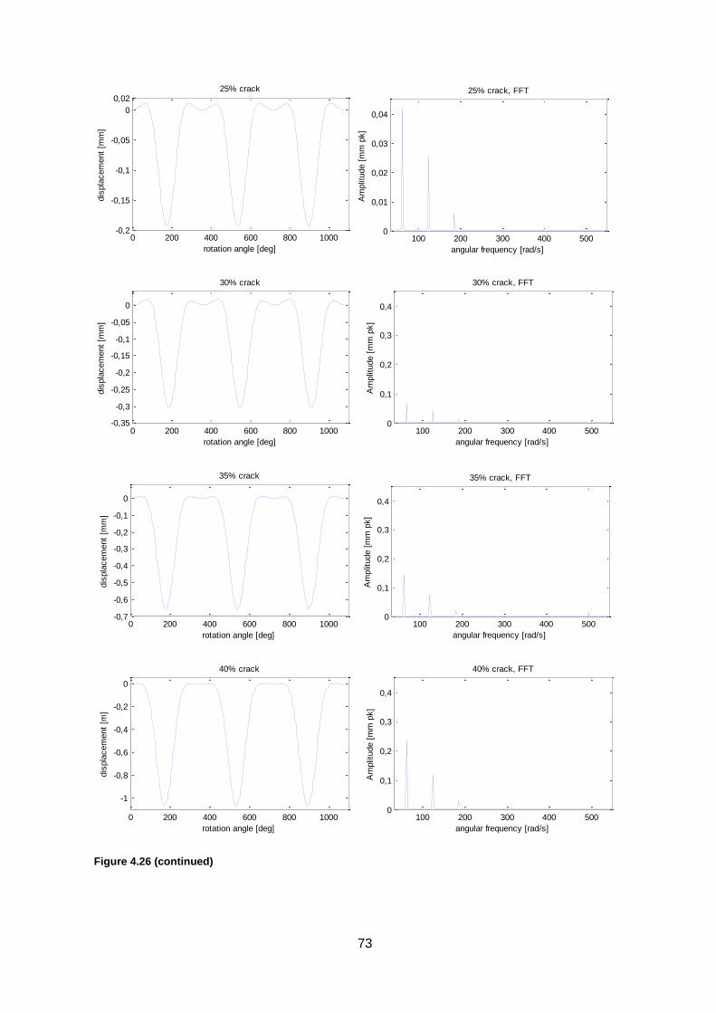
73
Figure 4.26 (continued)
0 200 400 600 800 1000-0,2
-0,15
-0,1
-0,05
0
0,0225% crack
rotation angle [deg]
dis
pla
cem
ent
[mm
]
100 200 300 400 5000
0,01
0,02
0,03
0,04
25% crack, FFT
angular frequency [rad/s]
Am
plit
ude [
mm
pk]
0 200 400 600 800 1000-0,35
-0,3
-0,25
-0,2
-0,15
-0,1
-0,05
0
30% crack
rotation angle [deg]
dis
pla
cem
ent
[mm
]
100 200 300 400 5000
0,1
0,2
0,3
0,4
angular frequency [rad/s]
Am
plit
ude [
mm
pk]
30% crack, FFT
0 200 400 600 800 1000-0,7
-0,6
-0,5
-0,4
-0,3
-0,2
-0,1
0
35% crack
rotation angle [deg]
dis
pla
cem
ent
[mm
]
100 200 300 400 5000
0,1
0,2
0,3
0,4
angular frequency [rad/s]
Am
plit
ude [
mm
pk]
35% crack, FFT
0 200 400 600 800 1000
-1
-0,8
-0,6
-0,4
-0,2
0
40% crack
rotation angle [deg]
dis
pla
cem
ent
[m]
100 200 300 400 5000
0,1
0,2
0,3
0,4
angular frequency [rad/s]
Am
plit
ude [
mm
pk]
40% crack, FFT
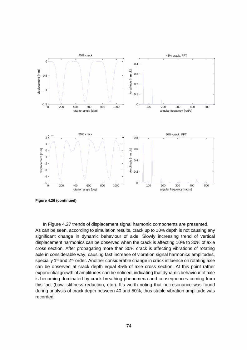
74
Figure 4.26 (continued)
In Figure 4.27 trends of displacement signal harmonic components are presented.
As can be seen, according to simulation results, crack up to 10% depth is not causing any
significant change in dynamic behaviour of axle. Slowly increasing trend of vertical
displacement harmonics can be observed when the crack is affecting 10% to 30% of axle
cross section. After propagating more than 30% crack is affecting vibrations of rotating
axle in considerable way, causing fast increase of vibration signal harmonics amplitudes,
specially 1st and 2nd order. Another considerable change in crack influence on rotating axle
can be observed at crack depth equal 45% of axle cross section. At this point rather
exponential growth of amplitudes can be noticed, indicating that dynamic behaviour of axle
is becoming dominated by crack breathing phenomena and consequences coming from
this fact (bow, stiffness reduction, etc.). It’s worth noting that no resonance was found
during analysis of crack depth between 40 and 50%, thus stable vibration amplitude was
recorded.
0 200 400 600 800 1000-1,5
-1
-0,5
0
45% crack
rotation angle [deg]
dis
pla
cem
ent
[mm
]
100 200 300 400 5000
0,1
0,2
0,3
0,4
angular frequency [rad/s]
Am
plit
ude [
mm
pk]
45% crack, FFT
0 200 400 600 800 1000-5
-4
-3
-2
-1
0
1
2x 10
-3 50% crack
rotation angle [deg]
dis
pla
cem
ent
[mm
]
100 200 300 400 5000
0,2
0,4
0,6
0,8
angular frequency [rad/s]
Am
plit
ude [
mm
pk]
50% crack, FFT
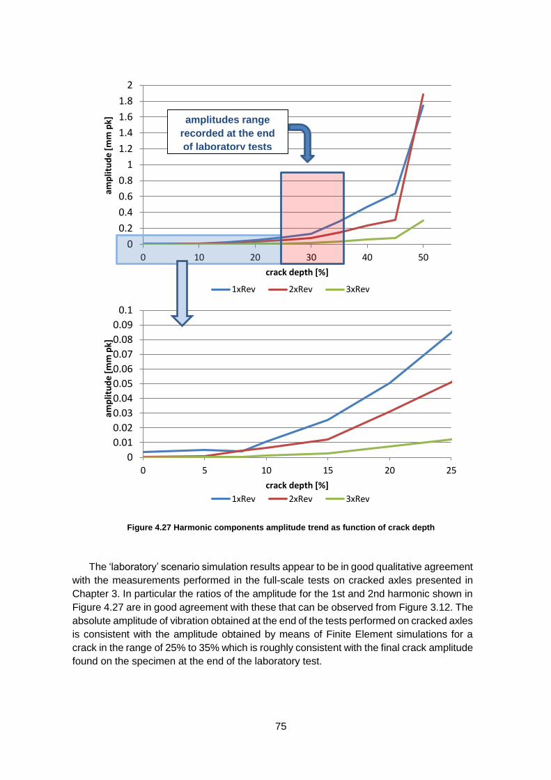
75
Figure 4.27 Harmonic components amplitude trend as function of crack depth
The ‘laboratory’ scenario simulation results appear to be in good qualitative agreement
with the measurements performed in the full-scale tests on cracked axles presented in
Chapter 3. In particular the ratios of the amplitude for the 1st and 2nd harmonic shown in
Figure 4.27 are in good agreement with these that can be observed from Figure 3.12. The
absolute amplitude of vibration obtained at the end of the tests performed on cracked axles
is consistent with the amplitude obtained by means of Finite Element simulations for a
crack in the range of 25% to 35% which is roughly consistent with the final crack amplitude
found on the specimen at the end of the laboratory test.
0
0.2
0.4
0.6
0.8
1
1.2
1.4
1.6
1.8
2
0 10 20 30 40 50
amp
litu
de
[m
m p
k]
crack depth [%]
1xRev 2xRev 3xRev
0
0.01
0.02
0.03
0.04
0.05
0.06
0.07
0.08
0.09
0.1
0 5 10 15 20 25
amp
litu
de
[mm
pk]
crack depth [%]
1xRev 2xRev 3xRev
amplitudes range
recorded at the end
of laboratory tests
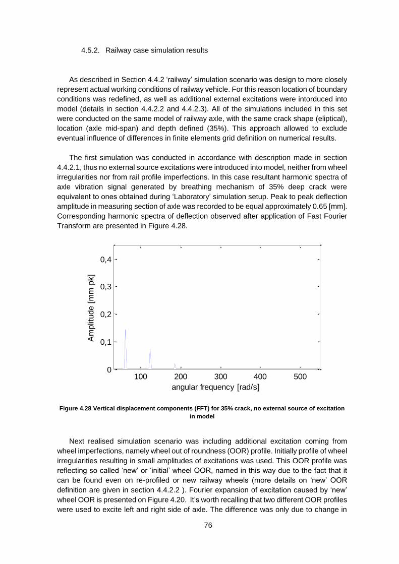
76
4.5.2. Railway case simulation results
As described in Section 4.4.2 ‘railway’ simulation scenario was design to more closely
represent actual working conditions of railway vehicle. For this reason location of boundary
conditions was redefined, as well as additional external excitations were intorduced into
model (details in section 4.4.2.2 and 4.4.2.3). All of the simulations included in this set
were conducted on the same model of railway axle, with the same crack shape (eliptical),
location (axle mid-span) and depth defined (35%). This approach allowed to exclude
eventual influence of differences in finite elements grid definition on numerical results.
The first simulation was conducted in accordance with description made in section
4.4.2.1, thus no external source excitations were introduced into model, neither from wheel
irregularities nor from rail profile imperfections. In this case resultant harmonic spectra of
axle vibration signal generated by breathing mechanism of 35% deep crack were
equivalent to ones obtained during ‘Laboratory’ simulation setup. Peak to peak deflection
amplitude in measuring section of axle was recorded to be equal approximately 0.65 [mm].
Corresponding harmonic spectra of deflection observed after application of Fast Fourier
Transform are presented in Figure 4.28.
Figure 4.28 Vertical displacement components (FFT) for 35% crack, no external source of excitation
in model
Next realised simulation scenario was including additional excitation coming from
wheel imperfections, namely wheel out of roundness (OOR) profile. Initially profile of wheel
irregularities resulting in small amplitudes of excitations was used. This OOR profile was
reflecting so called ‘new’ or ‘initial’ wheel OOR, named in this way due to the fact that it
can be found even on re-profiled or new railway wheels (more details on ‘new’ OOR
definition are given in section 4.4.2.2 ). Fourier expansion of excitation caused by ‘new’
wheel OOR is presented on Figure 4.20. It’s worth recalling that two different OOR profiles
were used to excite left and right side of axle. The difference was only due to change in
100 200 300 400 5000
0,1
0,2
0,3
0,4
angular frequency [rad/s]
Am
plit
ude [
mm
pk]
35% crack, FFT
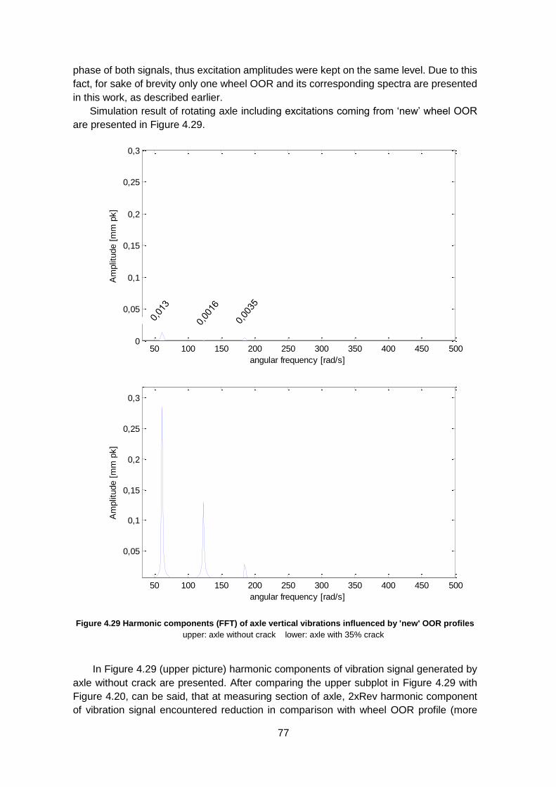
77
phase of both signals, thus excitation amplitudes were kept on the same level. Due to this
fact, for sake of brevity only one wheel OOR and its corresponding spectra are presented
in this work, as described earlier.
Simulation result of rotating axle including excitations coming from ‘new’ wheel OOR
are presented in Figure 4.29.
Figure 4.29 Harmonic components (FFT) of axle vertical vibrations influenced by 'new' OOR profiles
upper: axle without crack lower: axle with 35% crack
In Figure 4.29 (upper picture) harmonic components of vibration signal generated by
axle without crack are presented. After comparing the upper subplot in Figure 4.29 with
Figure 4.20, can be said, that at measuring section of axle, 2xRev harmonic component
of vibration signal encountered reduction in comparison with wheel OOR profile (more
50 100 150 200 250 300 350 400 450 5000
0,05
0,1
0,15
0,2
0,25
0,3
angular frequency [rad/s]
Am
plit
ude [
mm
pk]
NO CRACK + OOR, FFT new
50 100 150 200 250 300 350 400 450 500
0,05
0,1
0,15
0,2
0,25
0,3
angular frequency [rad/s]
Am
plit
ude [
mm
pk]
35% crack + OOR, FFT new
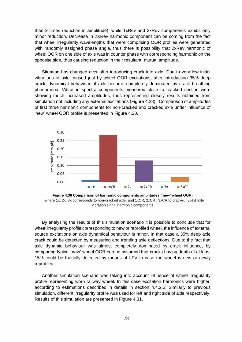
78
than 3 times reduction in amplitude), while 1xRev and 3xRev components exhibit only
minor reduction. Decrease in 2XRev harmonic component can be coming from the fact
that wheel irregularity wavelengths that were comprising OOR profiles were generated
with randomly assigned phase angle, thus there is possibility that 2xRev harmonic of
wheel OOR on one side of axle was in counter phase with corresponding harmonic on the
opposite side, thus causing reduction in their resultant, mutual amplitude.
Situation has changed over after introducing crack into axle. Due to very low initial
vibrations of axle caused just by wheel OOR excitations, after introduction 35% deep
crack, dynamical behaviour of axle became completely dominated by crack breathing
phenomena. Vibration spectra components measured close to cracked section were
showing much increased amplitudes, thus representing closely results obtained from
simulation not including any external excitations (Figure 4.28). Comparison of amplitudes
of first three harmonic components for non-cracked and cracked axle under influence of
‘new’ wheel OOR profile is presented in Figure 4.30.
Figure 4.30 Comparison of harmonic components amplitudes (‘new’ wheel OOR)
where 1x, 2x, 3x corresponds to non-cracked axle, and 1xCR, 2xCR , 3xCR to cracked (35%) axle
vibration signal harmonic components
By analysing the results of this simulation scenario it is possible to conclude that for
wheel irregularity profile corresponding to new or reprofiled wheel, the influence of external
source excitations on axle dynamical behaviour is minor. In that case a 35% deep axle
crack could be detected by measuring and trending axle deflections. Due to the fact that
axle dynamic behaviour was almost completely dominated by crack influence, by
comparing typical ‘new’ wheel OOR can be assumed that cracks having depth of at least
15% could be fruitfully detected by means of LFV in case the wheel is new or newly
reprofiled.
Another simulation scenario was taking into account influence of wheel irregularity
profile representing worn railway wheel. In this case excitation harmonics were higher,
according to estimations described in details in section 4.4.2.2. Similarly to previous
simulation, different irregularity profile was used for left and right side of axle respectively.
Results of this simulation are presented in Figure 4.31.
0.00
0.05
0.10
0.15
0.20
0.25
0.30
1
amp
litu
de
[mm
pk]
1x 1xCR 2x 2xCR 3x 3xCR
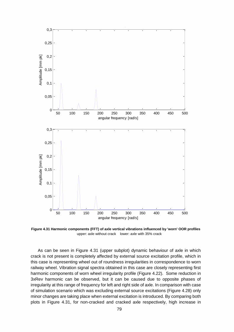
79
Figure 4.31 Harmonic components (FFT) of axle vertical vibrations influenced by 'worn' OOR profiles
upper: axle without crack lower: axle with 35% crack
As can be seen in Figure 4.31 (upper subplot) dynamic behaviour of axle in which
crack is not present is completely affected by external source excitation profile, which in
this case is representing wheel out of roundness irregularities in correspondence to worn
railway wheel. Vibration signal spectra obtained in this case are closely representing first
harmonic components of worn wheel irregularity profile (Figure 4.22). Some reduction in
3xRev harmonic can be observed, but it can be caused due to opposite phases of
irregularity at this range of frequency for left and right side of axle. In comparison with case
of simulation scenario which was excluding external source excitations (Figure 4.28) only
minor changes are taking place when external excitation is introduced. By comparing both
plots in Figure 4.31, for non-cracked and cracked axle respectively, high increase in
50 100 150 200 250 300 350 400 450 5000
0,05
0,1
0,15
0,2
0,25
0,3
angular frequency [rad/s]
Am
plit
ude [
mm
pk]
NO CRACK + OOR, FFT worn2
50 100 150 200 250 300 350 400 450 5000
0,05
0,1
0,15
0,2
0,25
0,3
angular frequency [rad/s]
Am
plit
ude [
mm
pk]
35% CRACK + OOR, FFT worn2
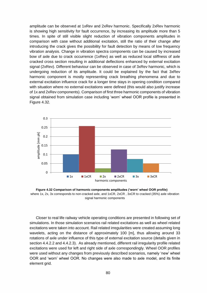
80
amplitude can be observed at 1xRev and 2xRev harmonic. Specifically 2xRev harmonic
is showing high sensitivity for fault occurrence, by increasing its amplitude more than 5
times. In spite of still visible slight reduction of vibration components amplitudes in
comparison with case without additional excitation, still the ratio of their change after
introducing the crack gives the possibility for fault detection by means of low frequency
vibration analysis. Change in vibration spectra components can be caused by increased
bow of axle due to crack occurrence (1xRev) as well as reduced local stiffness of axle
cracked cross section resulting in additional deflections enhanced by external excitation
signal (2xRev). Different behaviour can be observed in case of 3xRev harmonic, which is
undergoing reduction of its amplitude. It could be explained by the fact that 3xRev
harmonic component is mostly representing crack breathing phenomena and due to
external excitation influence crack for a longer time stays in opening condition compared
with situation where no external excitations were defined (this would also justify increase
of 1x and 2xRev components). Comparison of first three harmonic components of vibration
signal obtained from simulation case including ‘worn’ wheel OOR profile is presented in
Figure 4.32.
Figure 4.32 Comparison of harmonic components amplitudes (‘worn’ wheel OOR profile)
where 1x, 2x, 3x corresponds to non-cracked axle, and 1xCR, 2xCR , 3xCR to cracked (35%) axle vibration
signal harmonic components
Closer to real life railway vehicle operating conditions are presented in following set of
simulations. In those simulation scenarios rail related excitations as well as wheel related
excitations were taken into account. Rail related irregularities were created assuming long
wavelets, acting on the distance of approximately 100 [m], thus allowing around 33
rotations of axle under influence of this type of external excitation source (details given in
section 4.4.2.2 and 4.4.2.3). As already mentioned, different rail irregularity profile related
excitations were used for left and right side of axle correspondingly. Wheel OOR profiles
were used without any changes from previously described scenarios, namely ‘new’ wheel
OOR and ‘worn’ wheel OOR. No changes were also made to axle model, and its finite
element grid.
0
0.05
0.1
0.15
0.2
0.25
0.3
1
amp
litu
de
[mm
pk]
harmonic components1x 1xCR 2x 2xCR 3x 3xCR
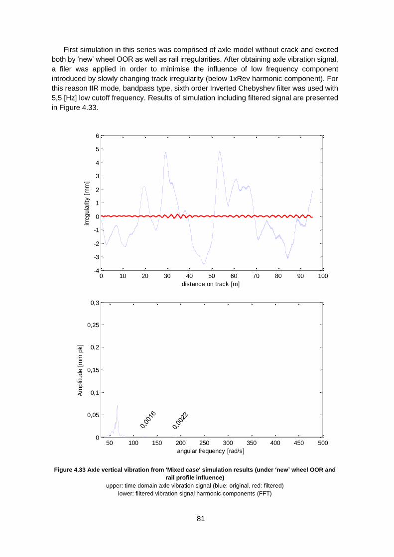
81
First simulation in this series was comprised of axle model without crack and excited
both by ‘new’ wheel OOR as well as rail irregularities. After obtaining axle vibration signal,
a filer was applied in order to minimise the influence of low frequency component
introduced by slowly changing track irregularity (below 1xRev harmonic component). For
this reason IIR mode, bandpass type, sixth order Inverted Chebyshev filter was used with
5,5 [Hz] low cutoff frequency. Results of simulation including filtered signal are presented
in Figure 4.33.
Figure 4.33 Axle vertical vibration from 'Mixed case' simulation results (under ‘new’ wheel OOR and
rail profile influence)
upper: time domain axle vibration signal (blue: original, red: filtered)
lower: filtered vibration signal harmonic components (FFT)
0 10 20 30 40 50 60 70 80 90 100-4
-3
-2
-1
0
1
2
3
4
5
6
distance on track [m]
irre
gula
rity
[m
m]
NO CRACK + RAILOOR, filtered new
50 100 150 200 250 300 350 400 450 5000
0,05
0,1
0,15
0,2
0,25
0,3
angular frequency [rad/s]
Am
plit
ude [
mm
pk]
NO CRACK +RAILOOR , FFT filtered new
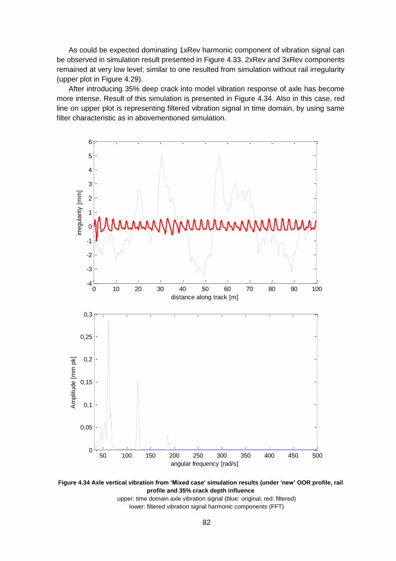
82
As could be expected dominating 1xRev harmonic component of vibration signal can
be observed in simulation result presented in Figure 4.33. 2xRev and 3xRev components
remained at very low level; similar to one resulted from simulation without rail irregularity
(upper plot in Figure 4.29).
After introducing 35% deep crack into model vibration response of axle has become
more intense. Result of this simulation is presented in Figure 4.34. Also in this case, red
line on upper plot is representing filtered vibration signal in time domain, by using same
filter characteristic as in abovementioned simulation.
Figure 4.34 Axle vertical vibration from ‘Mixed case' simulation results (under ‘new’ OOR profile, rail
profile and 35% crack depth influence
upper: time domain axle vibration signal (blue: original, red: filtered)
lower: filtered vibration signal harmonic components (FFT)
0 10 20 30 40 50 60 70 80 90 100-4
-3
-2
-1
0
1
2
3
4
5
6
distance along track [m]
irre
gula
rity
[m
m]
35% crack + RAILOOR +filtered new
50 100 150 200 250 300 350 400 450 5000
0,05
0,1
0,15
0,2
0,25
0,3
angular frequency [rad/s]
Am
plit
ude [
mm
pk]
35% crack +RAILOOR, FFT (filt) new
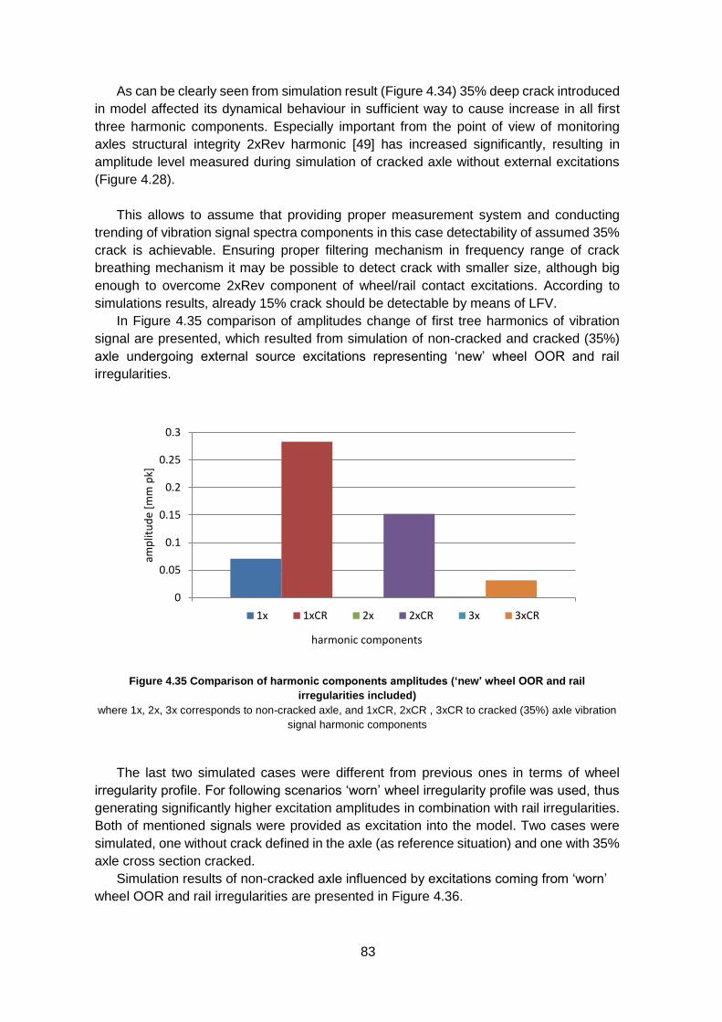
83
As can be clearly seen from simulation result (Figure 4.34) 35% deep crack introduced
in model affected its dynamical behaviour in sufficient way to cause increase in all first
three harmonic components. Especially important from the point of view of monitoring
axles structural integrity 2xRev harmonic [49] has increased significantly, resulting in
amplitude level measured during simulation of cracked axle without external excitations
(Figure 4.28).
This allows to assume that providing proper measurement system and conducting
trending of vibration signal spectra components in this case detectability of assumed 35%
crack is achievable. Ensuring proper filtering mechanism in frequency range of crack
breathing mechanism it may be possible to detect crack with smaller size, although big
enough to overcome 2xRev component of wheel/rail contact excitations. According to
simulations results, already 15% crack should be detectable by means of LFV.
In Figure 4.35 comparison of amplitudes change of first tree harmonics of vibration
signal are presented, which resulted from simulation of non-cracked and cracked (35%)
axle undergoing external source excitations representing ‘new’ wheel OOR and rail
irregularities.
Figure 4.35 Comparison of harmonic components amplitudes (‘new’ wheel OOR and rail
irregularities included)
where 1x, 2x, 3x corresponds to non-cracked axle, and 1xCR, 2xCR , 3xCR to cracked (35%) axle vibration
signal harmonic components
The last two simulated cases were different from previous ones in terms of wheel
irregularity profile. For following scenarios ‘worn’ wheel irregularity profile was used, thus
generating significantly higher excitation amplitudes in combination with rail irregularities.
Both of mentioned signals were provided as excitation into the model. Two cases were
simulated, one without crack defined in the axle (as reference situation) and one with 35%
axle cross section cracked.
Simulation results of non-cracked axle influenced by excitations coming from ‘worn’
wheel OOR and rail irregularities are presented in Figure 4.36.
0
0.05
0.1
0.15
0.2
0.25
0.3
1
amp
litu
de
[mm
pk]
harmonic components
1x 1xCR 2x 2xCR 3x 3xCR
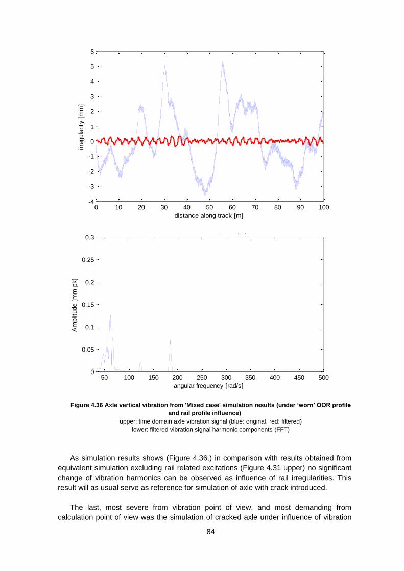
84
Figure 4.36 Axle vertical vibration from 'Mixed case' simulation results (under ‘worn’ OOR profile
and rail profile influence)
upper: time domain axle vibration signal (blue: original, red: filtered)
lower: filtered vibration signal harmonic components (FFT)
As simulation results shows (Figure 4.36.) in comparison with results obtained from
equivalent simulation excluding rail related excitations (Figure 4.31 upper) no significant
change of vibration harmonics can be observed as influence of rail irregularities. This
result will as usual serve as reference for simulation of axle with crack introduced.
The last, most severe from vibration point of view, and most demanding from
calculation point of view was the simulation of cracked axle under influence of vibration
0 10 20 30 40 50 60 70 80 90 100-4
-3
-2
-1
0
1
2
3
4
5
6
distance along track [m]
irre
gula
rity
[m
m]
NO CRACK + RAILOOR +filt worn2
50 100 150 200 250 300 350 400 450 5000
0.05
0.1
0.15
0.2
0.25
0.3
angular frequency [rad/s]
Am
plit
ude [
mm
pk]
NO CRACK + RAILOOR, FFT (filt) worn2
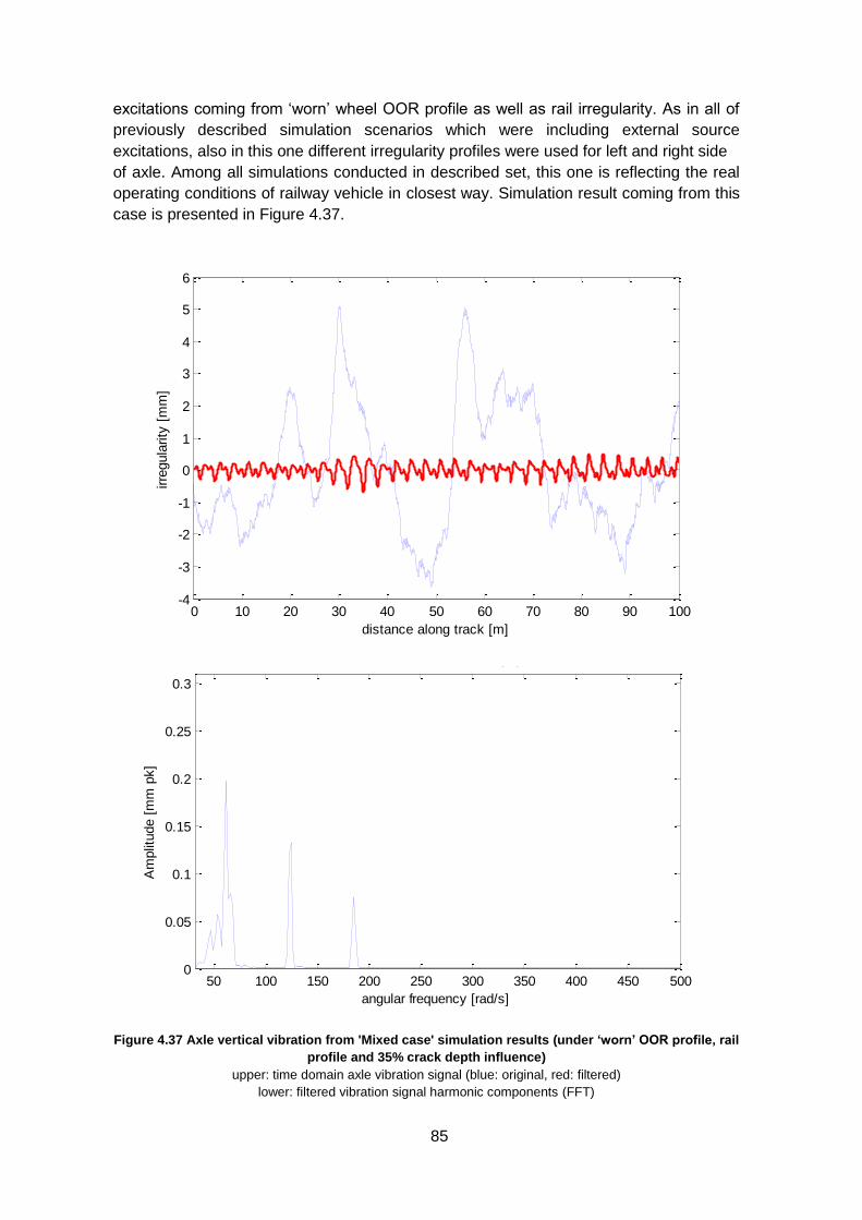
85
excitations coming from ‘worn’ wheel OOR profile as well as rail irregularity. As in all of
previously described simulation scenarios which were including external source
excitations, also in this one different irregularity profiles were used for left and right side
of axle. Among all simulations conducted in described set, this one is reflecting the real
operating conditions of railway vehicle in closest way. Simulation result coming from this
case is presented in Figure 4.37.
Figure 4.37 Axle vertical vibration from 'Mixed case' simulation results (under ‘worn’ OOR profile, rail
profile and 35% crack depth influence)
upper: time domain axle vibration signal (blue: original, red: filtered)
lower: filtered vibration signal harmonic components (FFT)
0 10 20 30 40 50 60 70 80 90 100-4
-3
-2
-1
0
1
2
3
4
5
6
distance along track [m]
irre
gula
rity
[m
m]
35% CRACK + RAILOOR +filt worn2
50 100 150 200 250 300 350 400 450 5000
0.05
0.1
0.15
0.2
0.25
0.3
Am
plit
ude [
mm
pk]
angular frequency [rad/s]
35% CRACK + RAILOOR, FFT (filt) worn2
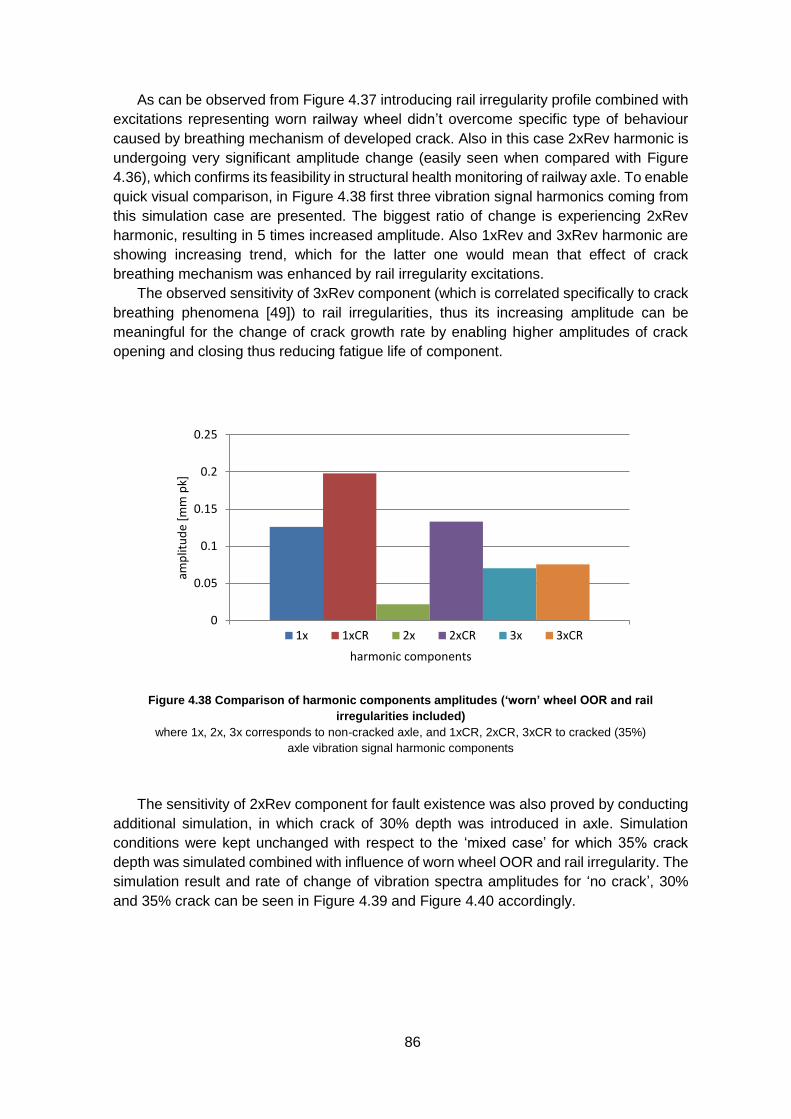
86
As can be observed from Figure 4.37 introducing rail irregularity profile combined with
excitations representing worn railway wheel didn’t overcome specific type of behaviour
caused by breathing mechanism of developed crack. Also in this case 2xRev harmonic is
undergoing very significant amplitude change (easily seen when compared with Figure
4.36), which confirms its feasibility in structural health monitoring of railway axle. To enable
quick visual comparison, in Figure 4.38 first three vibration signal harmonics coming from
this simulation case are presented. The biggest ratio of change is experiencing 2xRev
harmonic, resulting in 5 times increased amplitude. Also 1xRev and 3xRev harmonic are
showing increasing trend, which for the latter one would mean that effect of crack
breathing mechanism was enhanced by rail irregularity excitations.
The observed sensitivity of 3xRev component (which is correlated specifically to crack
breathing phenomena [49]) to rail irregularities, thus its increasing amplitude can be
meaningful for the change of crack growth rate by enabling higher amplitudes of crack
opening and closing thus reducing fatigue life of component.
Figure 4.38 Comparison of harmonic components amplitudes (‘worn’ wheel OOR and rail
irregularities included)
where 1x, 2x, 3x corresponds to non-cracked axle, and 1xCR, 2xCR, 3xCR to cracked (35%)
axle vibration signal harmonic components
The sensitivity of 2xRev component for fault existence was also proved by conducting
additional simulation, in which crack of 30% depth was introduced in axle. Simulation
conditions were kept unchanged with respect to the ‘mixed case’ for which 35% crack
depth was simulated combined with influence of worn wheel OOR and rail irregularity. The
simulation result and rate of change of vibration spectra amplitudes for ‘no crack’, 30%
and 35% crack can be seen in Figure 4.39 and Figure 4.40 accordingly.
0
0.05
0.1
0.15
0.2
0.25
1
amp
litu
de
[mm
pk]
harmonic components
1x 1xCR 2x 2xCR 3x 3xCR
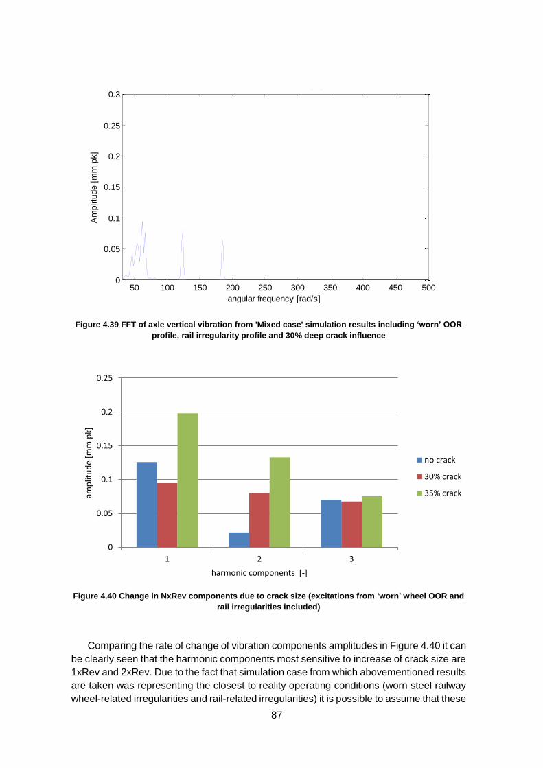
87
Figure 4.39 FFT of axle vertical vibration from 'Mixed case' simulation results including ‘worn’ OOR
profile, rail irregularity profile and 30% deep crack influence
Figure 4.40 Change in NxRev components due to crack size (excitations from ‘worn’ wheel OOR and
rail irregularities included)
Comparing the rate of change of vibration components amplitudes in Figure 4.40 it can
be clearly seen that the harmonic components most sensitive to increase of crack size are
1xRev and 2xRev. Due to the fact that simulation case from which abovementioned results
are taken was representing the closest to reality operating conditions (worn steel railway
wheel-related irregularities and rail-related irregularities) it is possible to assume that these
50 100 150 200 250 300 350 400 450 5000
0.05
0.1
0.15
0.2
0.25
0.330% crack + RAILOOR, FFT (filt) worn2
Am
plit
ude [
mm
pk]
angular frequency [rad/s]
0
0.05
0.1
0.15
0.2
0.25
1 2 3
amp
litu
de
[mm
pk]
harmonic components [-]
no crack
30% crack
35% crack

88
vibration components are the most suitable to enable proper estimation of structural
integrity of railway axle.
Simulations including additional sources of excitation coming from wheel-rail
interaction showed that irregularity levels reported on worn railway wheels are not
overcoming vibrations caused by 35% deep crack in the axle, thus allowing to assume
that the detection of a crack in similar size is highly probable during vehicle service. 1xRev
and 2xRev harmonics occurred to be the most suitable to indicate presence of crack.
Comparison of two cases with different crack depth (30% and 35%) revealed that NxRev
vibration components are undergoing higher rate of change of amplitude due to crack
propagation than from developing OOR profile of wheel allowing to assume that that axle
condition monitoring based on LFV is capable of delivering diagnostic results even during
further degradation of wheel profile.
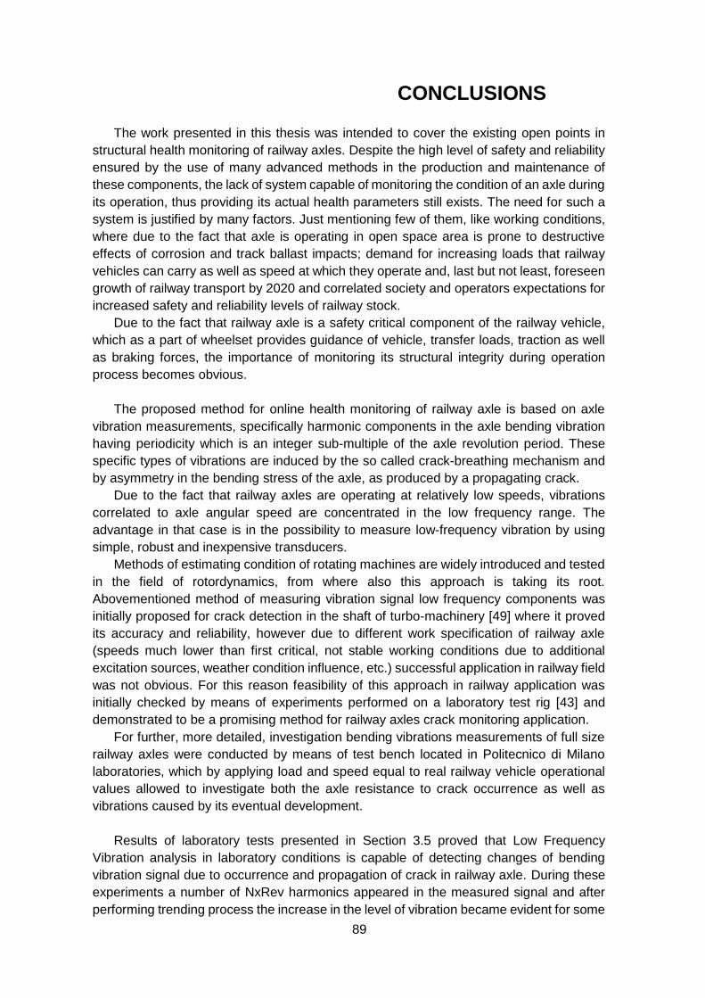
89
CONCLUSIONS
The work presented in this thesis was intended to cover the existing open points in
structural health monitoring of railway axles. Despite the high level of safety and reliability
ensured by the use of many advanced methods in the production and maintenance of
these components, the lack of system capable of monitoring the condition of an axle during
its operation, thus providing its actual health parameters still exists. The need for such a
system is justified by many factors. Just mentioning few of them, like working conditions,
where due to the fact that axle is operating in open space area is prone to destructive
effects of corrosion and track ballast impacts; demand for increasing loads that railway
vehicles can carry as well as speed at which they operate and, last but not least, foreseen
growth of railway transport by 2020 and correlated society and operators expectations for
increased safety and reliability levels of railway stock.
Due to the fact that railway axle is a safety critical component of the railway vehicle,
which as a part of wheelset provides guidance of vehicle, transfer loads, traction as well
as braking forces, the importance of monitoring its structural integrity during operation
process becomes obvious.
The proposed method for online health monitoring of railway axle is based on axle
vibration measurements, specifically harmonic components in the axle bending vibration
having periodicity which is an integer sub-multiple of the axle revolution period. These
specific types of vibrations are induced by the so called crack-breathing mechanism and
by asymmetry in the bending stress of the axle, as produced by a propagating crack.
Due to the fact that railway axles are operating at relatively low speeds, vibrations
correlated to axle angular speed are concentrated in the low frequency range. The
advantage in that case is in the possibility to measure low-frequency vibration by using
simple, robust and inexpensive transducers.
Methods of estimating condition of rotating machines are widely introduced and tested
in the field of rotordynamics, from where also this approach is taking its root.
Abovementioned method of measuring vibration signal low frequency components was
initially proposed for crack detection in the shaft of turbo-machinery [49] where it proved
its accuracy and reliability, however due to different work specification of railway axle
(speeds much lower than first critical, not stable working conditions due to additional
excitation sources, weather condition influence, etc.) successful application in railway field
was not obvious. For this reason feasibility of this approach in railway application was
initially checked by means of experiments performed on a laboratory test rig [43] and
demonstrated to be a promising method for railway axles crack monitoring application.
For further, more detailed, investigation bending vibrations measurements of full size
railway axles were conducted by means of test bench located in Politecnico di Milano
laboratories, which by applying load and speed equal to real railway vehicle operational
values allowed to investigate both the axle resistance to crack occurrence as well as
vibrations caused by its eventual development.
Results of laboratory tests presented in Section 3.5 proved that Low Frequency
Vibration analysis in laboratory conditions is capable of detecting changes of bending
vibration signal due to occurrence and propagation of crack in railway axle. During these
experiments a number of NxRev harmonics appeared in the measured signal and after
performing trending process the increase in the level of vibration became evident for some
90
of them. As the result of test, it was possible to observe that the most sensitive for crack
occurrence are the 1xRev to 3xRev harmonics. The 1xRev component showed the largest
increase in amplitude at the final stage of the tests along with the 2xRev component which
proved to be also sensitive to the number of cumulated loading blocks. The 3xRev
harmonic component also experienced almost monotonic increase but its trend was less
clear, probably on account of disturbances such as thermal effects that may produce a
bow of the rotating axle and thus reduce the breathing mechanism by keeping the crack
partially opened during revolutions.
Due to the fact that finally the 1xRev and 2xRev components allowed to assume that
they are the most promising indicators of eventual fault development in the axle, their
amplitudes measured at axles which experienced crack propagation were plotted at Figure
3.13 and Figure 3.14 for 1xRev and 2xRev harmonic respectively.
After obtaining promising results from laboratory tests numerical, 3D finite element
model of axle was created to enable investigation of influence of crack depth to dynamics
of railway axle under different working conditions.
Simulation campaign was divided into two parts, first one covering conditions found in
laboratory tests, and second one investigating possible vibrations levels that can occur
during train operation (thus taking into account additional sources of disturbance).
Due to the fact that railway wheels and rails are undergoing wear effects, thus
introducing additional excitations to the axle coming from the wheel-rail contact, the
influence of these excitations on crack breathing phenomena was under biggest concern.
Results of simulations representing laboratory conditions appeared to be in a good
qualitative agreement with measurements performed in the full – scale tests on cracked
axles. Specifically 1st and 2nd harmonic showed highest sensitivity for crack presence and
its size, which is also consistent with laboratory measurements results. The amplitude
levels obtained by means of Finite Element model for a crack size in a range of 25% to
35% of axle cross section were consistent with vibration amplitudes recorded during final
stage of laboratory tests, when crack was undergoing high propagation ratio.
So called ‘track’ case simulations including additional sources of excitation coming
from wheel-rail interaction revealed that even for irregularity levels reported on worn
railway wheels (dominating 1st and 3rd harmonic) still vibrations caused by 35% deep crack
were visible, thus allowing to assume that the detection of a crack having a size in thus
order of magnitude is highly probable despite the disturbances acting on the wheel during
real service. 1xRev and 2xRev harmonics occurred to be the most suitable to indicate
presence of crack. This is also true specifically when further degradation of wheel
circumference is considered, due to the fact that as simulations and field measurements
are showing [103] during increasing wear of wheel, OOR harmonics tends to develop into
higher orders leaving 2xRev harmonic slightly affected or causing reduction in its
amplitude.
Finally, nevertheless of possible influence of wheel OOR irregularity on NxRev
vibration component, the latter ones are undergoing higher rate of change of amplitude
due to crack propagation and thus affecting vibration signal to a larger extent than the
introduced by more slowly developing OOR thus opening the way to properly assess the
structural integrity of the axle.
Observing the actual developments in railway auxiliary systems, the energy harvesting
method from rotating railway axles seems to serve a good platform for implementation of

91
LFV measurement system. Due to the fact that equipment for both these systems will be
located at the axle side bearings reduction in additional space requirements, as well as
implementation costs can be achieved.
LFV application for monitoring structural integrity of railway axles can possibly be
extended to monitor wheel OOR profiles and track quality (latter one when LFV is
combined with GPS interface) due to their mutual influence on axle vibration levels.
92
ACKNOWLEDGEMENTS
The SHM results shown in the present research were obtained in the frame of the
SUSTRAIL Collaborative European Project (Grant Agreement #265740). The full-scale
crack propagation test is carried out in the frame of the MARAXIL Project co-funded by
Regione Lombardia (ID 16973, Rif. n° MAN-15).
The author would like to thank Prof. Stefano Bruni, Prof. Stefano Beretta, Dr Michele
Carboni and Ing. Mauro De Mori from Mechanical Engineering Department at Politecnico
di Milano for the help and useful discussions.
93
BIBLIOGRAPHY:
[1] "Railway Safety Performance in the European Union 2014," European Railway
Agency2014.
[2] C. Ulianov, F. Defossez, G. V. Franklina, and M. Robinson, "Overview of freight
train derailments in the EU. Causes, impacts, prevention and mitigation
measures," in Transport Research Arena (TRA) 5th Conference: Transport
Solutions from Research to Deployment, 2014.
[3] "Railway Investigation Report R10T0035," The Transportation Safety Board of
Canada (TSB)2010.
[4] "Summary report and database of derailments incidents," D-RAIL European
Project 05/04/2012 2012.
[5] CEN, "EN13261: Railway applications - Wheelsets and bogies - Axles - Product
requirements," ed, 2011.
[6] G. Mancini, A. Corbizi, F. Lombardo, and S. Cervello, "Design of railway axle in
compliance with the European Norms: high strength alloyed steels compared to
standard steels," in Proceedings of WCRR, 2006.
[7] (2014) Safety of the railway axle: the last mile of EURAXLES. European Railway
Review. 47-49.
[8] CEN, "EN 13103: Railway applications - Wheelsets and bogies - Non powered
axles - Design method," ed, 2012.
[9] CEN, "EN 13104: Railway applications - Wheelsets and bogies - Powered axles -
Design method," ed, 2011.
[10] CEN, "EN 13260: Railway applications - Wheelsets and bogies - Wheelsets -
Product requirements ", ed, 2010.
[11] D. Regazzi, "Advances in life prediction and durability of railway axles," 2014.
[12] B. Hänel, E. Haibach, T. Seeger, G. Wirthgen, and H. Zenner, "FKM-Guideline–
Analytical strength assessment of components in mechanical engineering,"
Forschungskuratorium Maschinenbau eV (FKM), Research Association for
Mechanical Engineering, Frankfurt, 2003.
[13] M. A. Miner, "Cumulative damage in fatigue," Journal of applied mechanics, vol.
12, pp. 159-164, 1945.
[14] E. Haibach, Modifizierte lineare Schadensakkumulations-hypothese zur
Berücksichtigung des Dauerfestigkeitsabfalls mit fortschreitender Schädigung:
Laboratorium für Betriebsfestigkeit, 1970.
[15] A. S. Watson, "Technical Challenges in the Axle Safety Model," Predicting real
world axle failure and reliability ed, 2011.
[16] S. Beretta, M. Carboni, G. Fiore, and A. L. Conte, "Corrosion–fatigue of A1N
railway axle steel exposed to rainwater," International Journal of fatigue, vol. 32,
pp. 952-961, 2010.
[17] C. Osgood, "Damage-tolerant design(Safe-life and fail-safe structural design
philosophies in fatigue damage and operating lifetime control)," Machine Design,
vol. 41, pp. 91-95, 1969.
[18] J. COMBES, RICHARD C, "Design for damage tolerance," Journal of Aircraft, vol.
7, pp. 18-20, 1970.
94
[19] U. Zerbst, M. Vormwald, C. Andersch, K. Mädler, and M. Pfuff, "The development
of a damage tolerance concept for railway components and its demonstration for
a railway axle," Engineering fracture mechanics, vol. 72, pp. 209-239, 2005.
[20] U. Zerbst, R. Lundén, K.-O. Edel, and R. A. Smith, "Introduction to the damage
tolerance behaviour of railway rails–a review," Engineering fracture mechanics,
vol. 76, pp. 2563-2601, 2009.
[21] S. Beretta, M. Carboni, and S. Cervello, "Design review of a freight railway axle:
fatigue damage versus damage tolerance," Materialwissenschaft und
Werkstofftechnik, vol. 42, pp. 1099-1104, 2011.
[22] S. Cantini, S. Beretta, and M. Carboni, "POD and inspection intervals of high speed
railway axles," in Proc. 15 th Int. Wheelset Congress, 2007.
[23] J. Rudlin, "Report on NDT performance (various techniques) for conventional
wheelsets. D6. 2.1: Inspection performance of axle inspection methods on existing
designs. D6. 2.2: use of inspection performance information for new axle design.
European project “Wheelset integrated design and effective
maintenance”(WIDEM), 2008," ed.
[24] Vereinigung der Privatgüterwagen-Interessenten (VPI, 2008): VPI Instandhaltungsleitfaden, Teil 06 Instandhaltung von Güterwagen – Zug- und Stoßeinrichtungen, 2. Ausgabe, gültig ab 01.02.2008.
[25] S. Beretta, M. Carboni, A. L. Conte, D. Regazzi, S. Trasatti, and M. Rizzi, "Crack
growth studies in railway axles under corrosion fatigue: Full-scale experiments and
model validation," Procedia Engineering, vol. 10, pp. 3650-3655, 2011.
[26] P. Monje, G. Aranguren, B. Martinez, and L. Casado, "Using bogie-mounted
sensors to measure wheel rolling and sliding on railway tracks," Proceedings of
the Institution of Mechanical Engineers, Part F: Journal of Rail and Rapid Transit,
vol. 226, pp. 371-380, 2012.
[27] A. Matsumoto, Y. Sato, H. Ohno, M. Tomeoka, K. Matsumoto, J. Kurihara, et al.,
"A new measuring method of wheel–rail contact forces and related
considerations," Wear, vol. 265, pp. 1518-1525, 2008.
[28] S. S. Bleakley and S. Senini, "Autonomous time frequency analysis of wagon body
accelerations," Faculty of Engineering and Physical Systems, Central Queensland
University, Rockhampton, Qld, Australia, 2004.
[29] R. Ngigi, C. Pislaru, A. Ball, and F. Gu, "Modern techniques for condition
monitoring of railway vehicle dynamics," in Journal of Physics: Conference Series,
2012, p. 012016.
[30] C. PENG, L. WANG, X. GAO, Z. WANG, Q. ZHAO, Y. ZHANG, et al., "High-Power
Locomotive Solid Axle Defect on-line Detection Technique."
[31] J. RUDLIN, A. RAUDE, U. VÖLZ, and A. L. CONTE, "New Methods of Rail Axle
Inspection and Assessment," in Proceedings of 18th World Conference on
Nondestructive Testing, 2012, pp. 16-20.
[32] V. Gorbunov and V. Sutorikhin, "Microwave Nondestructive Testing Method,"
Applied Physics Research, vol. 4, p. p206, 2012.
[33] R. Zoughi and S. Kharkovsky, "Microwave and millimetre wave sensors for crack
detection," Fatigue & Fracture of Engineering Materials & Structures, vol. 31, pp.
695-713, 2008.
[34] "Final Report Summary " WOLAXIM (Whole Life Rail Axle Assessment and
Improvement).
[35] C. U. Grosse and M. Ohtsu, Acoustic emission testing: Springer Science &
Business Media, 2008.
95
[36] M. Huang, L. Jiang, P. K. Liaw, C. R. Brooks, R. Seeley, and D. L. Klarstrom,
"Using acoustic emission in fatigue and fracture materials research," JOM, vol. 50,
pp. 1-14, 1998.
[37] C.-H. Jiang, W. You, L.-S. Wang, M. Chu, and N. Zhai, "Real-time monitoring of
axle fracture of railway vehicles by translation invariant wavelet," in Machine
Learning and Cybernetics, 2005. Proceedings of 2005 International Conference
on, 2005, pp. 2409-2413.
[38] L. Stepanova, A. Bobrov, S. Kabanov, and E. Y. Lebedev, "Enhancement of the
acoustic-emission method use for diagnostics of rolling stock cast parts," Russian
Journal of Nondestructive Testing, vol. 46, pp. 49-55, 2010.
[39] N. Thakkar, J. Steel, and R. Reuben, "Rail–wheel interaction monitoring using
Acoustic Emission: A laboratory study of normal rolling signals with natural rail
defects," Mechanical Systems and Signal Processing, vol. 24, pp. 256-266, 2010.
[40] S. Bekher and E. Tenitilov, "Dependence of the number of acoustic-emission
pulses on the mechanical testing load of bearing races in an axle unit," Russian
Journal of Nondestructive Testing, vol. 42, pp. 530-536, 2006.
[41] C.-H. Jiang, "A Fault Diagnosis System of Railway Vehicles Axle Based on
Translation Invariant Wavelet," in Machine Learning and Cybernetics, 2007
International Conference on, 2007, pp. 1045-1050.
[42] S. Bruni, M. Carboni, D. Crivelli, M. Guagliano, and P. Rolek, "A preliminary
analysis about the application of acoustic emission and low frequency vibration
methods to the structural health monitoring of railway axles," CHEMICAL
ENGINEERING, vol. 33, 2013.
[43] M. Carboni, S. Bruni, D. Crivelli, M. Guagliano, and P. Rolek, "A STUDY ON THE
PERFORMANCE OF ACOUSTIC EMISSION AND LOW FREQUENCY
VIBRATION METHODS TO THE REAL-TIME CONDITION MONITORING OF
RAILWAY AXLES."
[44] R. Morgan, K. Gonzales, E. Smith, and B. Smith, "Remotely detecting cracks in
moving freight railcar axles," 2006.
[45] K. Christian, N. Mureithi, A. Lakis, and M. Thomas, "On the use of time
synchronous averaging, independent component analysis and support vector
machines for bearing fault diagnosis," in First international conference on industrial
risk engineering, 2007.
[46] D. R. Houser and M. J. Drosjack, "Vibration Signal Analysis Techniques," DTIC
Document1973.
[47] I. Howard, "Vibration signal processing using MATLAB," ACOUSTICS
AUSTRALIA, vol. 23, pp. 9-9, 1995.
[48] R. Gasch, "A survey of the dynamic behaviour of a simple rotating shaft with a
transverse crack," Journal of sound and vibration, vol. 160, pp. 313-332, 1993.
[49] N. Bachschmid, P. Pennacchi, and E. Tanzi, Cracked rotors: a survey on static
and dynamic behaviour including modelling and diagnosis: Springer Science &
Business Media, 2010.
[50] R. T. Liong, Application of the cohesive zone model to the analysis of rotors with a
transverse crack vol. 16: KIT Scientific Publishing, 2012.
[51] A. Sanderson, "The vibration behaviour of a large steam turbine generator during
crack propagation through the generator rotor," in INSTITUTION OF
MECHANICAL ENGINEERS CONFERENCE PUBLICATIONS, 1992, pp. 263-
263.
96
[52] T. H. Patel and A. K. Darpe, "Influence of crack breathing model on nonlinear
dynamics of a cracked rotor," Journal of Sound and Vibration, vol. 311, pp. 953-
972, 2008.
[53] R. Gasch, "Dynamic behaviour of a simple rotor with a cross-sectional crack,"
presented at the IMechE Conf. Vibration in Rotating Machinery, Cambridge,UK,
1976.
[54] J. Wauer, "On the dynamics of cracked rotors: a literature survey," Applied
Mechanics Reviews, vol. 43, pp. 13-17, 1990.
[55] A. D. Dimarogonas, "Vibration of cracked structures: a state of the art review,"
Engineering fracture mechanics, vol. 55, pp. 831-857, 1996.
[56] G. Sabnavis, R. G. Kirk, M. Kasarda, and D. Quinn, "Cracked shaft detection and
diagnostics: a literature review," Shock and Vibration Digest, vol. 36, p. 287, 2004.
[57] C. Kumar and V. Rastogi, "A brief review on dynamics of a cracked rotor,"
International Journal of Rotating Machinery, vol. 2009, 2010.
[58] N. Bachschmid, P. Pennacchi, and E. Tanzi, "Some remarks on breathing
mechanism, on non-linear effects and on slant and helicoidal cracks," Mechanical
Systems and Signal Processing, vol. 22, pp. 879-904, 2008.
[59] I. Imam, S. Azzaro, R. Bankert, and J. Scheibel, "Development of an on-line rotor
crack detection and monitoring system," Journal of Vibration and Acoustics, vol.
111, pp. 241-250, 1989.
[60] T. Zhou, Z. Sun, J. Xu, and W. Han, "Experimental analysis of cracked rotor,"
Journal of dynamic systems, measurement, and control, vol. 127, pp. 313-320,
2005.
[61] O. Jun, H. Eun, Y. Earmme, and C.-W. Lee, "Modelling and vibration analysis of a
simple rotor with a breathing crack," Journal of Sound and vibration, vol. 155, pp.
273-290, 1992.
[62] J.-J. Sinou and A. Lees, "The influence of cracks in rotating shafts," Journal of
Sound and Vibration, vol. 285, pp. 1015-1037, 2005.
[63] G. Lapini, M. Zippo, N. Bachschmid, A. Collina, and A. Vallini, Experimental tests
and model based calculations for the diagnosis of a crack in 320 MW generator:
Springer, 1994.
[64] H. Ziebarth and R. Baumgartner, "Early detection of cross-sectional rotor cracks
by turbine shaft vibration monitoring techniques," ASME paper, pp. 4-8, 1981.
[65] J. H. Maxwell and D. A. Rosario, "Using modelling to predict vibration from a shaft
crack," Condition Monitoring and Diagnostic Engineering Management, Elsevier,
London, pp. 243-250, 2001.
[66] L. Nilsson, "On the vibration behaviour of a cracked rotor," in IFToMM International
Conference on Rotordynamic Problems in Power Plants, Rome, Italy, 1982, pp.
515-524.
[67] N. Bachschmid, P. Pennacchi, E. Tanzi, P. Verrier, F. Hasnaoui, and K. Aabadi,
"Crack detectability in vertical axis cooling pumps during operation," International
Journal of Rotating Machinery, vol. 10, pp. 121-133, 2004.
[68] P. P. Nicolò Bachschmid, Ezio Tanzi, Cracked Rotors. A Survey on Static and
Dynamic Behaviour Including Modelling and Diagnosis: Springer-Verlag Berlin
Heidelberg, 2010.
[69] A. Darpe, K. Gupta, and A. Chawla, "Coupled bending, longitudinal and torsional
vibrations of a cracked rotor," Journal of Sound and Vibration, vol. 269, pp. 33-60,
2004.
97
[70] I. Mayes and W. Davies, "Analysis of the response of a multi-rotor-bearing system
containing a transverse crack in a rotor," Journal of Vibration and Acoustics, vol.
106, pp. 139-145, 1984.
[71] C. A. Papadopoulos, "The strain energy release approach for modeling cracks in
rotors: A state of the art review," Mechanical systems and signal processing, vol.
22, pp. 763-789, 2008.
[72] C. Papadopoulos and A. Dimarogonas, "Coupled longitudinal and bending
vibrations of a rotating shaft with an open crack," Journal of sound and vibration,
vol. 117, pp. 81-93, 1987.
[73] O. Daoud and D. Cartwright, "Strain energy release rates for a straight-fronted
edge crack in a circular bar subject to bending," Engineering Fracture Mechanics,
vol. 19, pp. 701-707, 1984.
[74] J. T. Sawicki, M. I. Friswell, Z. Kulesza, A. Wroblewski, and J. D. Lekki, "Detecting
cracked rotors using auxiliary harmonic excitation," Journal of Sound and
Vibration, vol. 330, pp. 1365-1381, 2011.
[75] A.D.Dimarogonas, "Vibration of cracked structures: a state of the art review,"
Engineering Fracture Mechanics vol. 55 (5) pp. 831–857, 1996.
[76] A. D. Dimarogonas, S. A. Paipetis, and T. G. Chondros, Analytical methods in rotor
dynamics vol. 9: Springer Science & Business Media, 2013.
[77] Z. Kulesza and J. T. Sawicki, "Rigid finite element model of a cracked rotor,"
Journal of Sound and Vibration, vol. 331, pp. 4145-4169, 2012.
[78] R. T. Liong and C. Proppe, "Application of the cohesive zone model for the
evaluation of stiffness losses in a rotor with a transverse breathing crack," Journal
of Sound and Vibration, vol. 332, pp. 2098-2110, 2013.
[79] N. Bachschmid, P. Pennacchi, and E. Tanzi, "On the evolution of vibrations in
cracked rotors," in Proceedings of the 8th IFToMM International Conference on
Rotor Dynamics, 2010, pp. 304-310.
[80] Y.-S. Shih and J.-J. Chen, "Analysis of fatigue crack growth on a cracked shaft,"
International Journal of Fatigue, vol. 19, pp. 477-486, 1997.
[81] S. Beretta and M. Carboni, "Variable amplitude fatigue crack growth in a mild steel
for railway axles: experiments and predictive models," Engineering Fracture
Mechanics, vol. 78, pp. 848-862, 2011.
[82] "NI_9234 acquisition module data sheet," ed: National Instruments Corp. .
[83] H. Nyquist, "Certain topics in telegraph transmission theory," Proceedings of the
IEEE, vol. 90, pp. 280-305, 2002.
[84] C. E. Shannon, "Communication in the presence of noise," Proceedings of the
IEEE, vol. 72, pp. 1192-1201, 1984.
[85] A. Brandt, Noise and vibration analysis: signal analysis and experimental
procedures: John Wiley & Sons, 2011.
[86] A. V. Oppenheim, R. W. Schafer, and J. R. Buck, Discrete-time signal processing
vol. 2: Prentice-hall Englewood Cliffs, 1989.
[87] J. G. Proakis and D. K. Manolakis, Digital Signal Processing: Principles,
Algorithms, and Applications Prentice Hall, 2006.
[88] P. Brown, "Fundamental of Vibration Measurements and Analysis," ed: Lifetime
Reliability Solutions Application Note.
[89] D. M. Blunt, "Synchronous Averaging of Helicopter Tail Rotor Gearbox Vibration:
Phase Reference Considerations," DTIC Document1998.
98
[90] D. G. Manolakis and V. K. Ingle, Applied digital signal processing: theory and
practice: Cambridge University Press, 2011.
[91] R. B. Randall, Vibration-based condition monitoring: industrial, aerospace and
automotive applications: John Wiley & Sons, 2011.
[92] L. J. Brown, "Characterization of MSC/NASTRAN & MSC/ABAQUS elements for
turbine engine blade frequency analysis," presented at the Proc. MSC Aerospace
Users' Conference, 1997.
[93] "ABAQUS/Explicit (version 6.12) User's Manual (2012)," ed: Dassault Systemes.
[94] E. Q. Sun, "Shear locking and hourglassing in msc nastran, abaqus, and ansys,"
in Msc software users meeting, 2006.
[95] "Abaqus Explicit interface, User manual notes," ed: Dassault Systemes, 2005.
[96] E. Tarallo and G. Mastinu, "FE analysis with 3D elements," ed: POLITECNICO DI
MILANO, Dipartimento di Meccanica.
[97] "Abaqus Benchmarks Manual (6.12)," ed: Dassault Systemes, 2012.
[98] S. King and T. Richards, "Solving Contact Problems with Abaqus," ed: DS UK, Ltd,
Coventry, 2013.
[99] E. Chatzi and J. P. Escallon, "The Finite Element Method for the Analysis of Non-
Linear and Dynamic Systems; lecture notes," ed: Institute of Structural
Engineering, 2013.
[100] A. Kareem and K. Gurley, "Damping in structures: its evaluation and treatment of
uncertainty," Journal of Wind Engineering and Industrial Aerodynamics, vol. 59,
pp. 131-157, 1996.
[101] A. Alipour and F. Zareian, "Study Rayleigh damping in structures; unceratinties
and treatments," in Proceedings of 14th World Conference on Earthquake
Engineering, Beijing, China, 2008.
[102] J. F. Hall, "Problems encountered from the use (or misuse) of Rayleigh damping,"
Earthquake engineering & structural dynamics, vol. 35, pp. 525-545, 2006.
[103] J. C. Nielsen and A. Johansson, "Out-of-round railway wheels-a literature survey,"
Proceedings of the Institution of Mechanical Engineers, Part F: Journal of Rail and
Rapid Transit, vol. 214, pp. 79-91, 2000.
[104] A. Johansson and C. Andersson, "Out-of-round railway wheels—a study of wheel
polygonalization through simulation of three-dimensional wheel–rail interaction
and wear," Vehicle System Dynamics, vol. 43, pp. 539-559, 2005.
[105] G. Pallgen, "Unrunde Räder an Eisenbahnfahrzeugen: Durch ortsfeste
Messanlagen können unrunde Räder an Schienenfahrzeugen detektiert werden,"
Der Eisenbahningenieur, vol. 49, pp. 56-60, 1998.
[106] B. Morys and H.-B. Kuntze, "Simulation analysis and active compensation of the
out-of-round phenomena at wheels of high speed trains," in Proceedings of the
World Congress on Railway Research WCRR, 1997, pp. 16-19.

99