Low Frequency Transmission - Power Systems Engineering

Low Frequency Transmission

Final Project Report

Power Systems Engineering Research Center

Empowering Minds to Engineerthe Future Electric Energy System

Low Frequency Transmission

Final Project Report

Project Team

Faculty:

Sakis A. P. Meliopoulos, Project Leader Georgia Institute of Technology

Dionysios Aliprantis, Iowa State University

Graduate Research Assistants:

Yongnam Cho, Dongbo Zhao, and Anupama Keeli Georgia Institute of Technology

Hao Chen Iowa State University

PSERC Publication 12-28

October 2012

For information about this project, contact:

Sakis Meliopoulos

Georgia Power Distinguished Professor

School of Electrical and Computer Engineering

Georgia Institute of Technology

Atlanta, Georgia 30332-0250

Phone: 404-894-2926

E-mail: [email protected]


This is a project report from the Power Systems Engineering Research Center (PSERC).

PSERC is a multi-university Center conducting research on challenges facing a

restructuring electric power industry and educating the next generation of power

engineers. More information about PSERC can be found at the Center’s website:

http://www.pserc.wisc.edu.

For additional information, contact:


Arizona State University

527 Engineering Research Center

Tempe, Arizona 85287-5706

Phone: 480-965-1643

Fax: 480-965-0745

Notice Concerning Copyright Material

PSERC members are given permission to copy without fee all or part of this publication

for internal use if appropriate attribution is given to this document as the source material.

This report is available for downloading from the PSERC website.

2012 Georgia Institute of Technology and Iowa State University.

All rights reserved.

http://www.pserc.wisc.edu/

i

Acknowledgements

This is the final report for the Power Systems Engineering Research Center (PSERC)

research project S-42 titled “Low Frequency Transmission”. We express our appreciation

for the support provided by PSERC’s industrial members and by the National Science

Foundation’s Industry / University Cooperative Research Center program.

The authors wish to recognize their postdoctoral researchers and student graduate

research assistants (GRA) who contributed to the research and creation of the report:

Georgia Institute of Technology:

Yongnam Cho, GRA

Dongbo Zhao, GRA

Anupama Keeli, GRA

Iowa State University:

Hao Chen, GRA

The authors thank the following individuals for their technical advice on the project,

especially (the companies shown were as of time of this project work):

Bob Pierce, Duke Energy

Floyd Galvan and Shannon Watts, Entergy

Bruce Fardanesh and George Stefopoulos, New York Power Authority

Jianzhong Tong, PJM

Olivier Despouys, Sebastien Henry and Patrick Panciatici, RTE

Andrew Taylor, Southern Company Services Transmission Planning

i

Executive Summary

The goal of this project is to evaluate alternative transmission systems from remote wind

farms to the main grid using low-frequency AC technology. Low frequency means a

frequency lower than nominal frequency (60/50Hz). To minimize costs, cyclo-converter

technology is utilized resulting in systems of 20/16.66 Hz (for 60/50Hz systems

respectively). The technical and economic performance of low-frequency AC

transmission technology is compared to HVDC transmission and conventional AC

transmission in different configurations. The issue is quite important since wind potential

exists in remote and off-shore locations and the transmission system required to bring

wind energy to the main power grid represents a substantial expenditure of the overall

wind energy projects. The end result of this study is a comprehensive method for

evaluating and selecting the design parameters for alternative configurations of wind

projects and typical results of these evaluations for selected example systems.

In this project we have identified a number of possible configurations that are mainly

based on the three main options: (a) interconnection of a wind farm to the main power

grid via AC transmission, (b) interconnection of the wind farm to the main power grid via

DC transmission, and (c) interconnection of the wind farm to the main power grid via low

frequency AC transmission (LFAC). Using these three distinct transmission options,

eight alternative configurations were developed that include the above three options.

These alternative configurations were analyzed from several points of view. Specifically,

the following evaluations were performed: (a) optimal kV levels for each specific

alternative configuration, (b) reliability performance of each one of the alternative

configurations, (c) transfer capability of each one of the configurations, and (d) transient

stability analysis of each one of the configurations. For each one of these evaluations, a

parametric study has been performed when warranted. A summary for the final report is

provided below.

Chapter 1 provides an overview of the project and the reasons that the project was

initiated.

Chapter 2 provides an overview of the overall approach to the stated objectives for the

proposal. Specifically, the approach is based on developing comprehensive models for

the proposed technologies and to use these models to evaluate their performance and

compare them to competing technologies. The models developed are described in more

detail in the Appendices B and C.

Chapter 3 provides a literature survey for alternate connection methods of wind farm to

the main power grid using HVDC, conventional AC and LFAC technologies. Based on

the survey, eight alternate wind farm configurations have been proposed in Chapter 4 of

the report, including different combinations of in-farm technologies and out-farm

transmission technologies (HVDC, conventional AC or LFAC).

Chapter 4 describes alternative topologies for low-frequency transmission. Chapter 5

provides a methodology for determining the optimal kV level selection and equipment

rating. The selection methods are formulated based on the minimization of the total cost,

ii

which contains the operational cost and the acquisition cost. Specific analysis of the

selection of optimal kV level and equipment ratings based on the formulation of the total

cost for each of the eight proposed configurations has been performed. Examples of these

computations are provided in the section for each one of the eight alternative

configurations. The example results are summarized at the end of the chapter and

presented here. It should be emphasized that the values of the table below are valid only

for the considered example systems.

Configuration kV Level Selection Minimum Annualized Total Cost

(M$/year)

1 12 0.48

2 10 0.50

3 8 0.52

4 2 1.05

5 18 1.20

6 4 0.82

7 7 0.75

8 2 1.25

In Chapter 6, the operational study presents the comparison of maximum power transfer

capability between nominal-frequency systems and LFAC transmission systems. The

maximum power transfer capability is computed by gradually increasing the power

transfer until one of the operating constraints or static stability limits are violated. The

operational constraints are voltage limits, loading limits and electric current limits. The

stability constraints are the static stability limits. Example results are also presented for

specific example systems. For convenience we present one example of transmission at 76

kV below. The much higher power transfer capability of the low frequency AC system is

clearly apparent.

Maximum Transmission Capability at the Operation Voltage 76kV

Capability of Power Transmission (MW)

Distance

(miles) 10 30 50 70 90 100 120 140 160 180 200

Transfer

Capability

(MW) at

60Hz

180.3 82.8 57.54 44.17 36.78 34.31 30.56 27.98 26.19 24.84 23.38

Transfer

Capability

(MW) at

20Hz

225.3 141.3 106.1 86.28 73.49 68.29 60.19 54.27 49.22 45.21 41.96

iii

Chapter 7 describes the overall approach for performing transient analysis of wind farm

systems and provides case studies for voltage stability.

Chapters 8 and 9 describe the requirements for transient stability studies to determine the

suitability and operational robustness of these systems. These studies are important for

better understanding the dynamic behavior of these systems that include complex power

electronic systems. These studies also provide the generation of harmonics by these

systems. They are critical for understanding the harmonic content generated by wind

farms and LFAC transmission systems. The methods can be used to determine the need

for harmonic filters and if filters are needed, the method can be also used for the design

of these filters. Also, the power transient study allows the close observation of control

performance of power transients. Chapter 8 presents the overall approach for transient

analysis of the proposed low frequency AC transmission systems and presents the

controls of the power electronic subsystems for this operation. Design details for these

systems are also addressed, such as harmonic filter design, etc. Chapter 9 describes a

numerical integration of the basic models using the advanced quadratic integration.

Details of the simulation method are presented and results for specific systems are

presented. The ability of the proposed systems to control the power transferred and to

control the operation of these systems is demonstrated.

Chapter 10 provides an analysis of the eight alternative configurations from the reliability

point of view. Reliability analysis methods have been proposed for the alternative wind

farm configurations. Both the structural reliability model and the wind variability model

are considered in the reliability study. Monte Carlo models of the components and

probabilistic approaches of the topologies are utilized to formulate the reliability analysis

and reliability indices calculation. Case studies for each of the eight configurations are

provided and the reliability indices results are compared. Specifically, the reliability of

the wind farms is assessed in terms of the following reliability indices: EGWE (Expected

Generated Wind Energy) and CF (Capacity Factor). Results for example systems (one

example per proposed alternative configurations) are provided. A summary of these

results is given below for convenience.

Configuration EGWE IWP CF

1 22.98 60 0.383

2 22.42 60 0.374

3 20.82 60 0.347

4 26.22 60 0.437

5 12.31 60 0.205

6 25.86 60 0.431

7 20.54 60 0.342

8 26.27 60 0.438

iv

Conclusions and future work is discussed in Chapter 11. Since wind energy is the most

rapidly developed generating systems from all renewable resources and the forecast is

that they may be forming a large percentage of the generation system, their performance

is of paramount importance to the reliability of the power system of the near and far

future. The models developed in this research project can be utilized to study other very

important operational characteristics and capabilities of these systems. One main concern

is that as the percentage of wind generating systems become very large (even 100% in

some systems) what will be the operational challenges of these new systems from the

stability, control, operation and protection point of view. Suggestions are provided in

Chapter 11.

A total of four students contributed to this project (three at Georgia Tech and one at Iowa

State University. One Master’s thesis was written on the subject and two PhD theses were

written on the subject. In addition, nine publications were generated that describe the

work of this project. These publications and the three Theses (Dissertations) compliment

this main report.

Project Publications:

1. Yongnam Cho, Georgy J. Cokkinides, and A. P. Meliopoulos, “Time Domain

Simulation of a Three-Phase Cycloconverter for LFAC Transmission Systems,”

2012 IEEE Power and Energy Society Transmission and Distribution Conference

and Exhibition, Orlando, Florida, May 2012.

2. Yongnam Cho, George J. Cokkinides, A. P. Meliopoulos, “Transient Simulation

Technique for HVDC Systems,” in Proceedings of the International conference on

Power Systems Transients, Delft, the Netherlands, June 2011.

3. Yongnam Cho, George J. Cokkinides, A. P. Meliopoulos, “LFAC-Transmission

Systems for Remote Wind Farms Using a Three-phase, Six-pulse

Cycloconverter,” in Power Electronics and Machines in Wind Applications-

PEMWA 2012, Denver, Co, July 2012.

4. Yongnam Cho, Georgy J. Cokkinides, and A. P. Meliopoulos, “Advanced Time

Domain Method for Remote Wind Farms with LFAC Transmission Systems:

Power Transfer and Harmonics,” in North American Power Symposium, Urbana,

Illinois, September 2012.

5. Dongbo Zhao, A. P. Meliopoulos, George J. Cokkinides, Ramazan Caglar,

“Reliability Analysis of Alternate Wind Energy Farms and Interconnections,” in

Proceedings of 12th International Conf. on Probabilistic Methods Applied to

Power Systems, Istanbul, Turkey, June 2012.

6. Dongbo Zhao, A. P. Meliopoulos, Rui Fan, Zhenyu Tan and Yongnam Cho,

“Reliability Evaluation with Cost Analysis of Alternate Wind Energy Farms and

Interconnections,” in North American Power Symposium, Urbana, Illinois,

September 2012.

v

7. H. Chen, N. David, and D. C. Aliprantis, “Analysis of permanent magnet

synchronous generator with Vienna rectifier for wind energy conversion system,”

to appear in IEEE Trans. Sustainable Energy.

8. H. Chen and D. C. Aliprantis, “Analysis of squirrel-cage induction generator with

Vienna rectifier for wind energy conversion system,” IEEE Trans. Energy Conv.,

Vol. 26, No. 3, pp. 967-975, Sep. 2011.

9. H. Chen and D. C. Aliprantis, Induction generator with Vienna rectifier:

feasibility study for wind power generation," in Proc. IEEE Int. Conf. Electrical

Machines, Rome, Italy, Sep. 2010.

Student Theses and Dissertations:

1. Anupama, K. “Low Frequency Transmission for Remote Power Generating

Systems,” Master’s Thesis, Georgia Institute of Technology, 2011.

2. H. Chen, “Advances in Wind Power Generation, Transmission, and Simulation

Technology,” PhD dissertation, Iowa State University, Aug. 2012.

3. Yongnam Cho, “Transient Modeling of Converters for HVDC system and LFAC

Systems,” PhD dissertation, Georgia Institute of Technology, to be defended in

Spring 2013.

vi

Table of Contents

Acknowledgements .............................................................................................................. i

Executive Summary ............................................................................................................. i

Table of Contents ............................................................................................................... vi

List of Figures .................................................................................................................... ix

List of Tables .................................................................................................................... xv

1 Project Description ........................................................................................ 1

2 Technical Approach ...................................................................................... 3

3 Literature Survey ........................................................................................... 7

4 Alternative Topologies for Low-Frequency Transmission ........................... 9

4.1 Wind System Configuration 1: AC Wind Farm, Nominal Frequency, Network

Connection ................................................................................................................ 9

4.2 Wind System Configuration 2: AC Wind Farm, AC/DC Transmission, Network

Connection .............................................................................................................. 11

4.3 Wind System Configuration 3: Series DC Wind Farm, Nominal Frequency,

Network Connection ............................................................................................... 12

4.4 Wind System Configuration 4: Parallel Dc Wind Farm, Nominal Frequency,

Network Connection ............................................................................................... 13

4.5 Wind System Configuration 5: Series DC Wind Farm, Low Frequency Radial AC

Transmission ........................................................................................................... 15

4.6 Wind System Configuration 6: Parallel DC Wind Farm, Low Frequency, Radial

Transmission ........................................................................................................... 16

4.7 Wind System Configuration 7: Series DC Wind Farm, Low Frequency AC

Transmission Network ............................................................................................ 16

4.8 Wind System Configuration 8: Parallel DC Wind Farm, Low Frequency AC

Transmission Network ............................................................................................ 18

5 Optimal kV Level, Equipment Ratings and Cost Analysis of Alternate

Configurations ........................................................................................................ 19

5.1 Approach Description ............................................................................................. 19

5.2 kV Levels, Equipment Ratings and Wind Farm Cost Analysis

of Configuration 2 .................................................................................................. 32





vii

Table of Contents (continued)









5.9 Summary and Conclusions ..................................................................................... 58

6 Operational Studies – Power Transfer Capability ....................................... 59

6.1 Technical Approach of Power Transfer Capability Study ..................................... 59

6.2 Methodology for Simulation Models in Steady State ............................................ 60

6.3 Case Studies of Power-Transfer Capability ........................................................... 69

7 Transient Stability Studies .......................................................................... 73

7.1 Description and Technical Approach of Transient Stability Studies ..................... 73

7.2 Case Studies of Voltage-Stability Study ................................................................ 75

8 Time-Domain Studies-I ............................................................................... 83

8.1 System Configuration and Control ........................................................................ 83

8.2 Sending End Control .............................................................................................. 83

8.3 Receiving End Control ........................................................................................... 84

8.4 System Design ....................................................................................................... 87

8.5 Case Study ............................................................................................................. 92

8.6 Simulation Results ................................................................................................. 95

8.7 Conclusion ............................................................................................................. 98

9 Time-Domain Studies-II ............................................................................. 99

9.1 Technical Approach of Time-Domain Studies ...................................................... 99

9.2 Methodology for Simulation Models in Time-Domain ....................................... 101

9.3 Power-Transient Studies of LFAC Transmission Systems .................................. 121

9.4 Harmonics Study of LFAC Transmission Systems ............................................. 128

10 Reliability Analysis of Wind Farm Configurations .................................. 132

10.1 Approach Description .......................................................................................... 132

10.2 Reliability Analysis of Wind Farm Configuration 1 ............................................ 135

viii

Table of Contents (continued)








10.10 Summary and Conclusions .................................................................................. 174

11 Conclusions ............................................................................................... 175

Appendix A: Nomenclature .......................................................................................... 181

Appendix B: Example Wind Farm Model .................................................................... 183

Appendix C: Advanced Time-Domain Method (Quadratic) ........................................ 186

Appendix D: Reliability Model Parameters ................................................................. 191

Appendix E: Cost Parameters ....................................................................................... 193

ix

List of Figures

Figure 2.1: Typical Interconnection and Topology of Wind Farms and Collector

Substations .................................................................................................. 4

Figure 4.1.1: Wind System Configuration 1: AC Wind Farm, Nominal Frequency,

Network Connection ................................................................................. 10

Figure 4.2.1: Wind System Configuration 2: AC Wind Farm, AC/DC Transmission,

Network Connection ................................................................................. 11

Figure 4.3.1: Wind System Configuration 3: Series DC Wind Farm, Nominal

Frequency, Network Connection .............................................................. 12

Figure 4.4.1: Wind System Configuration 4: Parallel DC Wind Farm, Nominal

Frequency, Network Connection .............................................................. 14

Figure 4.5.1: Wind System Configuration 5: Series DC Wind Farm, Low Frequency

Radial AC Transmission ........................................................................... 15

Figure 4.6.1: Wind System Configuration 6: Parallel DC Wind Farm, Low Frequency,

Radial Transmission.................................................................................. 16

Figure 4.7.1: Wind System Configuration 7: Series DC Wind Farm, Low Frequency AC

Transmission Network .............................................................................. 17

Figure 4.8.1: Wind System Configuration 8: Parallel DC Wind Farm, Low Frequency

AC Transmission Network ....................................................................... 18

Figure 5.1.1: Alternative Configuration 1 - Example Configuration for Transmission

Loss Analysis ............................................................................................ 20

Figure 5.1.2: Acquisition Cost of Wind Turbine System vs. kV Level ......................... 27

Figure 5.1.3: Operating Cost of Example Configuration ............................................... 30

Figure 5.1.4: Annualized Acquisition Cost of Example Configuration ......................... 31

Figure 5.1.5: Annualized Total Cost of Example Configuration ................................... 32

Figure 5.2.1: Alternative Wind Farm Configuration 2 ................................................... 33

Figure 5.2.2: Annualized Total Cost of Configuration 2................................................ 36







x

List of Figures (continued)







Figure 6.1.1: Two Types of Transmission Configurations for Case Studies ................. 59

Figure 6.2.1: Three-Phase Transformer .......................................................................... 62

Figure 6.2.2: Three-Phase Overhead Transmission Line ............................................... 62

Figure 6.2.3: The Equivalent Circuit of a Single-Phase Transformer ............................ 63

Figure 6.2.4: The PI-Equivalent Circuit of a Single Phase Line .................................... 63

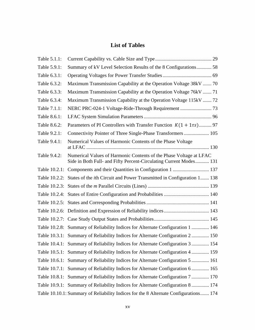
Figure 6.2.5: 115-kV Overhead Transmission Line: Left figure: equivalent circuit

at 60 Hz. Right figure: equivalent circuit at 20 Hz. .................................. 65





Figure 6.2.8: Power Electronic Systems (a) Three-Phase, Six-Pulse Converter,

(b) Three-Phase, PWM Converter, and (c) Three-Phase, Six-Pulse

Cycloconverter .......................................................................................... 67

Figure 6.3.1: Power Transmission Capability of the Operation Voltage 38-kV ............ 70

Figure 6.3.2: Power Transmission Capability of the Operation Voltage 76-kV ............ 71

Figure 6.3.3: Power Transmission Capability of the Operation Voltage 115-kV .......... 72

Figure 7.1.1: NERC PRC-024-1 Voltage-Ride-Through Requirement Curve ............... 74

Figure 7.2.1: Single-Line Diagram of a LFAC Transmission System Connecting

a Series LFAC Wind Farm to the Main Grid ............................................ 75

Figure 7.2.2: Configuration 1: Voltage Magnitude of Phase A at (A) Remote Grid

and (B) Local Grid, and (C) Before the Cycloconverter during a Three-

Phase Fault at Remote Grid ...................................................................... 76

Figure 7.2.3: Configuration 1: (A) Operating Frequency and (B) Real Power

at Remote Grid during a Three-Phase Fault at Remote Grid .................... 76

xi


Figure 7.2.4: Configuration 1: Voltage Magnitude of Phase A at (A) Remote Grid,

(B) Local Grid, and (C) Before the Cycloconverter during the Recloser

Operation................................................................................................... 77


at Remote Grid during the Recloser Operation ......................................... 77

Figure 7.2.6: Configuration 1: (A) Voltage Magnitude of Phase A and (B) Operating

Frequency during the Three-Phase Fault at Local Grid ............................ 78

Figure 7.2.7: Single-Line Diagram of LFAC Transmission Network Connecting

a Series DC Wind Farm ............................................................................ 79

Figure 7.2.8: Configuration 2: Voltage Magnitude of Phase A (A) at Remote Grid,

(B) at Local Grid 1, and (C) Before the Cycloconverter during a Three-

Phase Fault at Remote Grid ...................................................................... 80


at Remote Grid during a Three-Phase Fault at Remote Grid .................... 80

Figure 7.2.10: Configuration 2: Magnitude of Phase A Voltages at (A) Remote Grid

and (B) Local Grid 1, and (C) Real Power and Operating Frequency

at Remote Grid during a Three-Phase Fault at Local Grid 1 .................... 81

Figure 7.2.11: Configuration 2: Magnitude of Phase A voltages at (A) Remote Grid

and (B) Local Grid 1 during Recloser Operation

at RECLOSOR-LFAC2-TR ...................................................................... 82

Figure 7.2.12: Configuration 2: Magnitude of Phase A Voltages at (A) Remote Grid

and (B) Local Grid 1 during Recloser Operation

at RECLOSOR-LFAC1-TR ...................................................................... 82

Figure 8.1.1: Configuration of the Proposed LFAC Transmission System ................... 83

Figure 8.2.1: Sending End DC/AC Inverter Control ...................................................... 84

Figure 8.3.1: Receiving End Cycloconverter Control .................................................... 86

Figure 8.3.2: Details of the Signal Conditioning Block ................................................. 86

Figure 8.3.3: Modulator for Phase A .............................................................................. 87

Figure 8.4.1: Equivalent Circuit of 20 Hz Transmission System ................................... 90

Figure 8.4.2: Equivalent Circuit of 20 Hz Transmission System for Harmonic

Analysis..................................................................................................... 90

Figure 8.4.3: Harmonic Voltage Amplitudes Generated by the Cycloconverter

at the 20 Hz Side ....................................................................................... 92

Figure 8.5.1: Equivalent Circuit of 60 Hz Transmission System ................................... 93

xii


Figure 8.5.2: Sending End Active Power vs. Max. Transmission Distance ................... 94

Figure 8.5.3: Filter Design ....................................................................................... 95

Figure 8.5.4: Equivalent Impedance Magnitude Seen from the Receiving End ............ 95

Figure 8.6.1: Simulated Voltage and Current Waveforms ............................................. 97

Figure 8.6.2: Transient Waveforms ................................................................................ 98

Figure 9.1.1: Wind Farm Configuration: LFAC Wind Farm and LFAC

Transmission ........................................................................................... 100

Figure 9.1.2: Wind Farm Configuration: Series DC Wind Farm and LFAC

Transmission ........................................................................................... 100

Figure 9.2.1: (A) Three-Phase Y-Δ Isolation Transformer and (B) Single Phase

Transformer ............................................................................................. 102

Figure 9.2.2: Three-Phase, Six-Pulse Cycloconverter .................................................. 106

Figure 9.2.3: Electrical Valve ....................................................................................... 107

Figure 9.2.4: Circulating Current Circuit Model .......................................................... 108

Figure 9.2.5: Control Algorithm for the Cycloconverter ............................................. 111

Figure 9.2.6: Close Loop Control Algorithm for (a) Magnitude of Voltage and

(b) Output Power..................................................................................... 112

Figure 9.2.7: Three-Phase PWM Converter ................................................................. 114

Figure 9.2.8: Three-Phase PWM Converter ................................................................. 115

Figure 9.2.9: Constant-Frequency Controller using Direct-Power Algorithm

with Space-Vector Modulation ............................................................... 116

Figure 9.2.10: Variable-Frequency Controller using Direct-Power Algorithm

with Hysteresis Controllers ..................................................................... 116

Figure 9.2.11: Block Diagram of DPC Control Algorithm ............................................ 118

Figure 9.2.12: (A) SVM Diagram and (B) Mirror Image in SVM Diagram .................. 120

Figure 9.3.1: Wind Farm Configuration: LFAC Wind Farm and LFAC

Transmission ........................................................................................... 122

Figure 9.3.2: Three-Phase (a) Line-to-Line Voltages and (d) Currents at 60Hz AC

Transmission Connected to the Cycloconverter; Three-Phase (c) Voltages

and (b) Currents at LFAC Transmission Connected to the Cycloconverter;

and (e) Real Power from Wind Farm and (f) RMS Voltage at the LFAC

from 0.0 to 7.0 Seconds .......................................................................... 123

xiii


Figure 9.3.3: Three-Phase (a) Line-to-Line Voltage and (d) Currents at 60Hz AC


and (b) Currents at LFAC Transmission Connected to the

Cycloconverter; and (e) Real Power from Wind Farm and (f) RMS

Voltage at the LFAC from 2.8 to 3.4 Seconds ........................................ 123

Figure 9.3.4: Three-Phase (a) Line-to-Line Voltage and (d) Current at 60Hz AC


and (b) Currents at LFAC Transmission Connected to the Cycloconverter;

and (e) Real Power from Wind Farm and (f) RMS Voltage at the LFAC

from 6.75 to 7.0 Seconds ........................................................................ 124

Figure 9.3.5: Single-Line Diagram of a Power Transient Test System ........................ 125

Figure 9.3.6: (a) Three-Phase Line-to-Line Voltages and (b) Three-Phase Currents at

60Hz AC Transmission Connected to the Cycloconverter; Three-Phase

(c) Voltages and (b) Currents at LFAC Transmission Connected t

o the Cycloconverter; and (e) Real Power from Wind Farm and (f) RMS

Voltage at the LFAC from 0.0 to 8.0 Seconds ........................................ 126

Figure 9.3.7: (a) Three-Phase Line-to-Line Voltages and (b) Three-Phase Currents

at 60Hz AC Transmission Connected to the Cycloconverter; and Three-

Phase (c) Voltages and (b) Currents at LFAC Transmission Connected

to the Cycloconverter during Steady State from 4.846 to 5.0 Seconds .. 126

Figure 9.3.8: (a) Three-Phase Line-to-Line Voltages and (b) Three-Phase Currents

at 60Hz AC Transmission Connected to the Cycloconverter; Three-Phase

(c) Voltages and (b) Currents at LFAC Transmission Connected

to the Cycloconverter during Steady State from 9.785 to 8.0 Seconds .. 127

Figure 9.3.9: (a) Three-Phase Currents at 60Hz AC Transmission Connected

to the Cycloconverter; and Three-Phase (b) Voltages and (c) Currents

at LFAC Transmission Connected to the Cycloconverter during Steady

State from 0.0 to 0.500 Seconds. ............................................................ 127

Figure 9.3.10: (a) Three-Phase Currents at 60Hz AC Transmission Connected

to the Cycloconverter; and Three-Phase (b) Voltages and (c) Currents

at LFAC Transmission Connected to the Cycloconverter during Steady

State from 4.867 to 5.423 Seconds ......................................................... 128

Figure 9.4.1: (A) Line-to-Line Voltage between Phase A and Phase B; (B) Current

at Phase A; (C) Phase Voltage and (D) Phase Current at Phase A ......... 129

Figure 9.4.2: Harmonic Spectrums: (A) Line-to-Line Voltage between Phase A and

Phase B, (B) Current at Phase A, (C) Phase Voltage at Phase A, and

(D) Phase Current at Phase A ................................................................. 129

Figure 9.4.3: Harmonic Spectrums of the Phase Voltage at the LFAC Side ............... 130

xiv


Figure 9.4.4: Harmonic Spectrums of the Phase Voltage at the LFAC Side: (Blue) Full

Circulating-Current Mode and (Red) 50% Circulating-Current Mode ... 131

Figure 10.1.1: Wind Speed Probabilistic Distribution [27] ............................................ 134

Figure 10.1.2: A Typical Wind Turbine Output Considering Wind Speed Variation ... 134

Figure 10.2.1: Wind Farm Configuration 1 .................................................................... 136

Figure 10.2.2: A 30 WT Case Study Configuration for Configuration 1 ....................... 144








xv

List of Tables

Table 5.1.1: Current Capability vs. Cable Size and Type ............................................. 29

Table 5.9.1: Summary of kV Level Selection Results of the 8 Configurations ............ 58

Table 6.3.1: Operating Voltages for Power Transfer Studies ....................................... 69

Table 6.3.2: Maximum Transmission Capability at the Operation Voltage 38kV ....... 70



Table 7.1.1: NERC PRC-024-1 Voltage-Ride-Through Requirement ......................... 73

Table 8.6.1: LFAC System Simulation Parameters ...................................................... 96

Table 8.6.2: Parameters of PI Controllers with Transfer Function .......... 97

Table 9.2.1: Connectivity Pointer of Three Single-Phase Transformers .................... 105

Table 9.4.1: Numerical Values of Harmonic Contents of the Phase Voltage

at LFAC .................................................................................................. 130

Table 9.4.2: Numerical Values of Harmonic Contents of the Phase Voltage at LFAC

Side in Both Full- and Fifty Percent-Circulating Current Modes ........... 131

Table 10.2.1: Components and their Quantities in Configuration 1 ............................. 137

Table 10.2.2: States of the ith Circuit and Power Transmitted in Configuration 1 ....... 138

Table 10.2.3: States of the m Parallel Circuits (Lines) ................................................. 139

Table 10.2.4: States of Entire Configuration and Probabilities .................................... 140

Table 10.2.5: States and Corresponding Probabilities .................................................. 141

Table 10.2.6: Definition and Expression of Reliability indices .................................... 143

Table 10.2.7: Case Study Output States and Probabilities ............................................ 145

Table 10.2.8: Summary of Reliability Indices for Alternate Configuration 1 .............. 146








Table 10.10.1: Summary of Reliability Indices for the 8 Alternate Configurations ....... 174

1

1 Project Description

The project’s goal is to evaluate alternative transmission systems from remote wind farms

to the main grid using low-frequency AC technology. Low frequency means a frequency

lower than nominal frequency (60/50Hz). To minimize costs cyclo-converter technology

will be utilized resulting in systems of 20/16.66 Hz (for 60/50Hz systems respectively).

The technical and economic performance of low-frequency AC transmission technology

will be compared to HVDC transmission (including HVDC Light) and conventional AC

transmission. Electric power generation from wind is increasing at a fast rate. Plans to

install hundreds of GW of wind turbine generation in the next few years are in place in

the US, Europe, and China. Typically, geographic sites that are suitable for wind farm

development are in remote land locations or offshore locations, far from the main

transmission grid and major load centers. For instance, this is the case in the US, with

abundant wind potential in the scarcely populated Midwestern states, as well as for

offshore sites that could be located tens of miles from the coast. In these cases, the

transmission of wind power to the main grid is a major expenditure that adversely affects

the economics of these systems. The most economical approach depends on distance and

electric power (capacity) to be transmitted. Presently well-established technologies are

AC transmission or HVDC transmission (including HVDC Light). HVDC technology is

mature and offers significant advantages for long-distance point-to-point transmission, as

generally required by wind farm applications. However, one main disadvantage attributed

to HVDC is increased cost due to the complexity of the power electronics converters at

the two ends of the lines. HVDC Light technology tries to limit the cost but it is still

higher than AC technology. As a lower-cost alternative to HVDC or AC transmission, we

propose transmission by a low-frequency AC system, using thyristor-based AC/DC and

AC/AC converters. The proposed system is expected to have costs substantial lower than

HVDC – the cost savings will come from the fact that we propose to use cyclo-converters

which are much lower in cost than the typical six-pulse converters for HVDC. The

disadvantage of using cyclo-converters is that the frequency reduction is fixed – the most

practical system is 20 Hz. Other savings can come from optimizing the topology of the

wind farms. Another advantage of the proposed topologies is that existing transformers

designed for 60 Hz can be used for the proposed topologies (for example a 345kV/69 kV,

60Hz transformer can be used for a 115 kV/23kV, 20 Hz system). We propose to use

alternative topologies that will provide additional cost savings (operational and

investment cost) by minimizing the power electronic transformations. The proposed

configurations might indeed provide similar advantages to HVDC at reduced cost and

high reliability, therefore improving the financial viability of remote wind power plants.

The goal of this project is to perform a comprehensive evaluation of the technical

performance and economics of low-frequency AC transmission, in comparison to HVDC

and power-frequency AC transmission. It is expected that a comprehensive evaluation

may allow the industry to make better-informed decisions for the type of transmission for

large wind farm projects in remote inland or offshore sites. It is also expected that the

proposed topologies will enable a more comprehensive evaluation of storage at the wind

2

farm site, and will shape our thinking of the merits of storage in connection to wind

energy.

The major potential benefit from this technology will be a significant cost reduction of

the transmission system for remote or offshore wind farms (compared to the alternatives

of HVDC transmission or power-frequency AC transmission). This could make the

economics of wind energy more favorable, and aid our nation’s goal of 20% wind

penetration by 2030, by allowing utilities to tap into rich wind potential of remote

onshore or offshore areas. The proposed topologies have numerous operational benefits

as well, such as high reliability, capability of voltage and reactive power support, energy

storage, and enhanced dispatchability of the wind resource. The expected outcomes of the

project are: (a) a comprehensive methodology for determining the optimal topology, kV

levels, etc. of a low-frequency AC transmission system for wind farms and a given

distance of the wind farms from major power grid substations, (b) a monitoring and

control system for the proposed technologies that will allow enhanced dispatchability of

the wind resource and ability to provide ancillary services such as voltage and reactive

power support, and (c) a comprehensive methodology to evaluate the reliability of the

proposed topologies and the expected capacity credit of wind farms to the power grid.

This project will result in high-fidelity simulation models to analyze all different aspects

of the proposed low-frequency AC transmission technology for wind power plants.

PSERC industrial members could use these models to study the feasibility of such

configurations in their systems.

3

2 Technical Approach

The desirability of providing at least part of the required electric power from renewable

sources has made wind energy the leading renewable energy source because of the

favorable economics as compared to other renewables. Still there are few problems that

make wind energy economics higher than other forms of electric power generation. Two

main issues are: (a) the cost for transmission of wind power from remote sites where

large wind farms can be developed, and (b) the unpredictability of the wind that results in

low capacity credits for the operation of the integrated power system. We propose to

investigate alternative topologies and transmission systems operating at low frequency

for the purpose of decreasing the cost of transmission and making the wind farm a more

reliable power source so that the capacity credit can increase. The general approach for

defining these topologies is illustrated in Figure 2.1 which illustrates one alternative

configuration. Note that we envision that the configuration will include sections of DC

transmission as well as AC transmission and LF AC transmission, within and outside the

wind farm. This will enable to directly rectify the output of wind generators via a

standard transformer to DC of appropriate kV level. The system can be optimized

depending on the area covered by the wind farm. Storage can be provided at the DC bus.

While the proposed use of storage is not unique to the proposed low frequency

transmission, the proposed topology facilitates a more efficient and centralized utilization

of storage. An inverter can transform DC to AC of low frequency, preferably of 1/3 of the

normal power frequency. This low-frequency AC can be transformed to higher voltages

for transmission at higher kV levels. Standard transformers can be used as long as the

V/Hz operating value remains the same; for example, a 13.8kV/230kV 60 Hz transformer

can be used for 4.6kV/76.6kV 20 Hz operation. The low-frequency AC network will be

connected to the power grid at major substations via cyclo-converters that provide a low-

cost interconnection and synchronization with the main grid. The cost reduction enabled

with cyclo-converters is substantial as compared with HVDC options with the limitation

that the frequency reduction is fixed at 20 Hz. Transmission line design procedures

developed for 60 Hz systems can be equally applied to transmission lines operating at 20

Hz. Overall, 20 Hz transmission systems can be constructed with existing components

and technology. The proposed topologies will enable (a) optimization of the overall

transmission network for wind energy with substantial economic benefits, (b) a more

reliable operation because the number of conversion will be smaller (only one conversion

process per wind farm versus per wind turbine today), (c) a more dispatchable operation

of the wind farms since all wind turbines deposit their output to one DC bus (the net

output of many wind turbines is smoother than the output of a single wind turbine) plus

the storage on the DC bus will enable the overall wind farm to better respond to

dispatchers’ controls, and (d) the presence of the inverter and cyclo-converter will allow

the wind farm to provide ancillary services and in particular voltage and reactive power

control. The above-described basic approach can produce a number of alternative

topologies for specific geographical arrangements. In addition, it will allow the more

economical development of other forms of storage systems, such as hydro or pumped

hydro that may be located in remote areas.

4

Figure 2.1: Typical Interconnection and Topology of Wind Farms and Collector

Substations

Since there are competing technologies for transmission and storage, the proposed project

will be focusing on a comprehensive comparative evaluation of three competing

technologies: (a) AC transmission at power frequency (60 Hz or 50 Hz), (b) HVDC

transmission, including HVDC Light, and (c) the proposed low-frequency (20 Hz)

transmission topologies. The criteria for the comparative evaluation will be: (1) overall

cost—investment and operational cost, (2) voltage regulation/ reactive power control,

(3) fault currents, protection schemes and overall reliability, (4) dispatchability with and

without storage, (5) stability and transfer capability, (6) ability to provide ancillary

services to the main power grid, and (7) scalability. To minimize the system cost,

commercial off-the-shelf transformers designed for 60 Hz operation can be used in the 20

5

Hz transmission system. Simply, in order to maintain rated magnetic flux in their iron

cores, their nominal voltage ratings need to be scaled down by a factor of 3. For instance,

a 60 Hz 13.8kV/230kV transformer is de-rated to operate at 4.6kV/76.6kV at 20 Hz. In

addition, hysteresis and eddy current losses in the core are also significantly reduced, thus

increasing transmission efficiency. In particular, the use of the medium-voltage (a few

kVs) DC bus has the following advantages: (a) It allows for the easy interconnection of

a large battery energy storage system (BESS), which could be used to enable a more

predictable and dispatchable power output from the wind farm. The size of the BESS will

be a function of the stochastic nature of wind at the wind farm site, and of the power

system operators’ requirements for the plant’s maximum ramp down/up rates. The battery

technology (i.e., chemistry) also will have an impact on cost and efficiency.

(b) The AC/DC converters that connect each wind turbine to the DC bus represent some

very interesting control possibilities. Essentially, they may be considered as power

electronics drives, similar in principle to industrial motor drives, which decouple the

turbines’ terminal voltage magnitude and frequency from the nominal system values.

This forces us to re-think the design of wind turbine control schemes (designed to allow

variable-speed operation and maximum power point tracking). For all turbine generator

types (i.e., induction machines, wound-rotor and doubly-fed induction machines, or

synchronous machines), these converters can be controlled in such a way as to provide

maximum efficiency and energy capture from the wind. For instance, the converter’s AC

voltage and frequency could be varied (in some constant V/f fashion) to control the

turbine’s speed and/or minimize iron core losses in the transformer and generator,

thereby potentially eliminating the need for more advanced and expensive power

electronics that are found in DFIG and SG turbines (such as converters with AC-DC-AC

topologies). (c) The overall topology can be optimized independently from any other

systems, for example the DC-bus kV level can be optimally selected to minimize the

losses within the area of the wind farm. The size, design and controls of the low-

frequency inverter can be also optimized to enable efficient conversion, coordination with

storage, and ancillary services.

The comprehensive evaluation was performed as follows. First, test systems and specific

topologies were developed in collaboration with the industry advisors. The derived test

systems are described in Section 4. A total of eight different alternative configurations

were developed that include the alternative technologies, i.e. AC transmission, LFAC

transmission, DC transmission, DC wind farm distribution, AC wind farm distribution,

and series or parallel connection of wind turbine systems. For each one of the alternative

configurations a number of scenarios was developed. These scenarios include (a)

stochastic processes that define the time model of wind speeds at the various points of the

wind turbine systems, (b) stochastic processes that define the time model of marginal

power prices and demand for electric power at the interfacing substations to the main grid

(these processes will represent the overall operation of the power grid). The time scale for

simulation of these systems has been selected to be one year. For each one of the

alternative configurations and the scenarios of wind speeds and operations of the main

power grid, the following studies have been performed:

6

A. Operational analysis of the entire system on 15 minute intervals. The operational

analysis has been characterized with the following metrics: (1) voltage profile

index; (2) total transmission losses from wind turbines to the interconnecting

substations to the main power grid; (3) dispatchability index in terms of how

many MW can be dispatched if needed for the specific operating conditions and

wind speeds; (4) transfer capability index in terms of MW that can be transferred

over and above the operating conditions before violating constraints; (5) required

BESS size and cost.

B. Transient stability analysis, using average-value models of the converters’

operation. This analysis has been used: (1) to design the outer-loop high-level

controls used to interface the wind farm(s) with the power system, with particular

emphasis on the control infrastructure requirements, and the ability to provide

inertial frequency control and other ancillary services; (2) to study the stability of

the power system under contingencies; (3) to determine the transient

discharge/charge rates of the storage scheme and optimize its operation, and (4) to

study the ability of the system to provide voltage ancillary services to the power

grid under various conditions including shortcoming of reactive power in the grid,

delayed voltage recovery in the grid, and oscillatory voltage fluctuations.

C. Detailed EMTP-type simulation including switching events to analyze phenomena

with shorter time constants. This type of analysis has been used: (1) to design the

inner-loop controls at the power electronic converters; (2) to predict fault currents

under symmetric and asymmetric faults at the AC side, as well as short-circuits at

the DC bus (the most severe case); (3) to design the protective relaying system;

(4) to study the impact of harmonics on the system performance and cost. The

thyristor-based converters introduce low-frequency harmonics (compared to

IGBT-based converters that switch at much higher frequencies), and thus can

significantly degrade the system’s power quality; (5) to evaluate the harmonic

losses and power quality, and investigate the need for inclusion of harmonic

filters; (6) to study in detail the effects of communication delays between the two

ends of the transmission line (i.e., how they impact the protection system).

7

3 Literature Survey

The possible solutions for wind farm transmission are HVAC, Line commutated HVDC

and voltage source based HVDC (VSC-HVDC). The various wind farm designs have

been studied in the past with these technologies. In this study the low frequency AC

transmission technology is proposed for various designs of the wind farms.

The author in [1] presents an algorithm to derive a probabilistic wind turbine generator

model to determine the annual energy output of a wind farm connected to the grid. The

model focuses on generation and transmission system reliability and wind speed variation

is only considered as an occurrence probability. Thus the wind speed variation effect is

weakened in the evaluation. In the present study the total cost of the energy production

including the infrastructure and maintenance cost is evaluated. It is expected that the cost

of transmission and generation remains more or less the same compared to the previous

methods of transmission.

In reference [2] Thomas et al., proposed that a series connection of the wind farm leads to

the elimination of the offshore platform and the turbines output would be DC voltage. As

a result the desired transmission voltage can be obtained directly without a large

centralized DC/DC converter. Various wind farm designs with low frequency and

nominal frequency transmission are proposed in the study.

S. Lundberg in reference [7] proposed a control strategy for the series connected wind

turbines showing that the wind farm was able to operate successfully even though there

were large variations in the individual turbine powers. A key result of the study is that a

wind farm layout utilizing series connected wind turbines with a DC voltage output has a

very promising energy production cost, if the transmission distance is above 20 km. The

current study is concentrating on onshore as well as offshore power transmission

involving variable distances.

Cost of energy production of a wind turbine is an important element in this study. There

are many factors contributing to the cost and productivity of the wind farm. For low

frequency transmission the transmission cable as well as the related expenditure would be same

as for the nominal frequency transmission. In order for the wind farms to be economically

reasonable it is important to keep the energy production cost down. This can be done by

having a site with high average wind speed, a wind park layout that fits the site and to

keep the number of operation hours high. The energy production of various wind parks is

calculated in [17, 18, 19].

The estimated cost of the produced electric energy is presented in the references [20, 17,

21, 19, 23]. In [22], R. Barthelmie and S. Pryor presented the economics of some

offshore wind farms that are built and are planned to be built. The investment and

operational cost of the wind farm are investigated in this study. From this it can be said

that the cost of the cable can be determined by the number of cables, the transmission

voltage and the transmitted power by each cable.

8

In [24] the cost of cable per kilometer depending on the transmission voltage for the off-

shore wind farms is given. In this evaluation for cases with more than one line needing to

connect to onshore the author considered that all the submarine cables are installed

together. Different studies about the cost of energy based on the investments made and

the produced energy are carried out. These analyses are centered on the comparison

between AC and DC transmission. Particularly the analysis in [26] is based on very high

powers 400 – 100MW. As different transmission options are not considered in detail in

these studies the present study tries to complete the analysis.

9

4 Alternative Topologies for Low-Frequency Transmission

The literature survey indicates that many topologies and systems have been proposed for

transmitting power from wind farms to the main power grid. We have also proposed

variations of topologies that it is believed to have additional advantages. In this section

we present a number of topologies and systems that are further evaluated of their

advantages or shortcomings.

A wind farm is a group of a number of wind turbines located in the same geographical

area and interconnected. Individual wind turbines are interconnected with a medium

voltage power collection system. In order to connect the local wind turbine grid to the

transmission system the voltage is increased. Wind farm has the following elements:

wind turbines, local wind turbine grid, collecting point, transmission system, wind farm

interface to the point of common connection (PCC). The power from the wind turbine

units is collected at the collecting point where the voltage is increased to a level suitable

for transmission. The power is then transmitted to the wind farm grid interface over the

transmission system. The following are the different wind farm topologies.

4.1 Wind System Configuration 1: AC Wind Farm, Nominal Frequency, Network

Connection

Wind farms that have been built today have an AC electrical system from the wind

turbines to the PCC. Two different types of AC wind farms reffered in the study are

radial and network connections. The idea with the radial wind farm is that it should be

suitable for small wind farms with a short transmission distance. In the small AC wind

farm, the local wind farm grid is used both for connecting all wind turbines in a radial

fashion together and to transmit the generated power to the wind farm grid interface. The

other type of wind farm is the network connection. Large AC wind farms generally have

network connection of wind farms. In this type of configuration the local wind farm grid

has a lower voltage level than the transmission system. This system requires an offshore

platform for the transformer and switch gear. Horns Rev Wind Farm is built according to

this principle.

10

Figure 4.1.1: Wind System Configuration 1: AC Wind Farm, Nominal Frequency,

Network Connection

The wind system configuration shown in Figure 4.1.1 has an AC wind farm. The wind

turbines are connected in network fashion and nominal frequency transmission is

adopted. For the purpose of the study a network of 10 radial feeders is considered with 5

wind turbines in each feeder. Selection of the optimal voltage levels is described in

Section 5.

This configuration is described with the following parameters:

N: Number of radial feeders

Ni: Number of wind turbines in feeder i

d: Spacing between the wind turbines

Pt: Rating of the wind turbine

R: Resistance of the cable

kVdc: DC voltage level

In this configuration the wind turbines are interconnected with medium voltage. N, the

number of radial feeders and Ni, the number of wind turbines in the feeder i are decided

based on the total electrical output required from the wind farm. Wind turbines with

rating (Pt) 1MW, 1.75MW, 2.25MW or 3.6MW are considered in the study. Spacing

between the turbines d, is fixed based on the size of the wind turbine. As per

requirements the cable is chosen based on its resistance.

11

4.2 Wind System Configuration 2: AC Wind Farm, AC/DC Transmission,

Network Connection

In this system, the AC transmission is replaced with a DC transmission. This wind farm

will be referred to as the AC/DC wind farm. This type of system does not exist today, but

is frequently proposed when the distance to the PCC is long or if the AC grid that the

wind farm is connected to is weak. The system is shown in Figure 4.2.1. In this system

we have an independent local AC system in which both the voltage and the frequency are

fully controllable with the offshore converter station. This can be utilized for a collective

variable speed system of all wind turbines in the farm. The benefits with this are that the

aerodynamic and electrical efficiency can be increased.

Figure 4.2.1: Wind System Configuration 2: AC Wind Farm, AC/DC Transmission,

Network Connection

The wind system configuration shown in figure has a AC wind farm. The wind turbines

in the farm are connected in network fashion and DC transmission is adopted. Selection

of optimal voltage levels is described in Section 5.






12


kVdc: DC voltage level.

The AC wind farm configuration is similar to the wind system configuration 1 except for

the transmission part. The AC transmission is replaced by the DC transmission here.

4.3 Wind System Configuration 3: Series DC Wind Farm, Nominal Frequency,

Network Connection

The layout of the DC wind farm somewhat differs from the AC wind farm. The

difference is in the number transformation steps it requires to increase the DC voltage at

the local wind turbine grid to the level suitable for transmission. The number of

transformations depends on the DC voltage level in the local wind turbine grid. If the

voltage level is high i.e. 20-40kV DC then only one transformation step is required. But if

the output voltage of the wind turbine is lower i.e. 5kV, two steps are required. All wind

turbines within one cluster are connected one by one to the first transformation step. If

only one step is used, the wind turbines are connected in radials directly to the second DC

transformer step, similarly as for the AC wind farm.

Figure 4.3.1: Wind System Configuration 3: Series DC Wind Farm, Nominal

Frequency, Network Connection

13

The wind system configuration shown in figure has a DC wind farm. The wind turbines

are connected in network fashion and nominal frequency transmission is adopted.

Selection of the optimal voltage levels is described in Section 5.








The local wind farm is a DC wind farm and the wind turbines are connected in series. N,

the number of radial feeders and Ni, the number of wind turbines in the feeder i is

decided based on the total electrical output required from the wind farm. Wind turbines

with rating (Pt) 1MW, 1.75MW, 2.25MW or 3.6MW are considered in the study. Spacing



4.4 Wind System Configuration 4: Parallel Dc Wind Farm, Nominal Frequency,

Network Connection

The configuration differs from the wind system configuration 4 only in the local wind

farm. Here the wind turbines are connected in parallel. The wind system configuration

shown in figure 4.4.1 has a DC wind farm. The wind turbines are connected in network

fashion and nominal frequency transmission is adopted. Selection of the optimal voltage

levels is described in Section 5.

14

AC/DC

Converter

DC/AC Converter

DC Bus

AC/DC

Converter

DC/AC Converter

DC Bus

Power System

Power System

Figure 4.4.1: Wind System Configuration 4: Parallel DC Wind Farm, Nominal

Frequency, Network Connection








The local wind farm is a DC wind farm and the wind turbines are connected in parallel.

N, the number of radial feeders and Ni, the number of wind turbines in the feeder i is

decided based on the total electrical output required from the wind farm. Wind turbines

with rating (Pt) 1MW, 1.75MW, 2.25MW or 3.6MW are considered in the study. Spacing

15



4.5 Wind System Configuration 5: Series DC Wind Farm, Low Frequency Radial

AC Transmission

The proposed Low frequency AC transmission configuration would significantly reduce

the transmission system loss for remote or offshore wind farms. This makes the

economics of wind energy more favorable and increase the wind resources penetration

easy. Existing transmission line design, breakers and protection can be used and

cycloconverters offer an inexpensive conversion technology for conversion of frequency

from 60/50 Hz to 20/16.67Hz.

Figure 4.5.1: Wind System Configuration 5: Series DC Wind Farm, Low Frequency

Radial AC Transmission

Wind system configuration shown in the figure has a DC wind farm. The wind turbines

are connected in series, radial fashion and low frequency transmission is adopted.









The wind turbines in the local wind farm are connected in series. It has low frequency

transmission (20Hz/16.66Hz). The number of radial feeders is one. The total number of

wind turbines in the wind farm is decided depending upon the requirements of the

electrical output. The losses of the system are also to be taken into consideration while

designing the system.

16

4.6 Wind System Configuration 6: Parallel DC Wind Farm, Low Frequency,

Radial Transmission

The proposed system adopts low frequency of 20/16.67Hz. The wind system

configuration shown in figure has a DC wind farm. The wind turbines are connected in

parallel, radial fashion and low frequency transmission is adopted. Selection of the

optimal voltage levels is described in Section 5.

Figure 4.6.1: Wind System Configuration 6: Parallel DC Wind Farm, Low Frequency,

Radial Transmission








4.7 Wind System Configuration 7: Series DC Wind Farm, Low Frequency AC

Transmission Network


are connected in series, network fashion and low frequency transmission is adopted.


17

Figure 4.7.1: Wind System Configuration 7: Series DC Wind Farm, Low Frequency AC









18

4.8 Wind System Configuration 8: Parallel DC Wind Farm, Low Frequency AC



are connected in parallel, network fashion and low frequency transmission is adopted.


Figure 4.8.1: Wind System Configuration 8: Parallel DC Wind Farm, Low Frequency

AC Transmission Network








19

5 Optimal kV Level, Equipment Ratings and Cost Analysis of

Alternate Configurations

In this section, the optimal kV level and the equipment ratings for each alternate

configuration listed in Section 4 are discussed and analyzed. The optimal kV level for

transmission is selected on the basis of the minimum total cost consisting of operating

costs, maintenance costs and acquisition costs. In the analysis presented in this section we

consider mainly the transmission power loss cost and the acquisition cost. Maintenance

costs can be added but in general their influence in determining optimal kV levels is

small. Since the selection of optimal kV levels is dependent on total cost, this section

presents formulae for cost accounting for each wind farm configuration. Subsection 5.1

provides the general formulation of the methods used in the optimal kV level and

equipment ratings selection analysis, and cost analysis methods, using Configuration 1 as

the example. Subsequent subsections provide optimal kV level analysis, equipment

ratings, operational cost and acquisition cost analysis for each configurations listed in

Section 4. A 30 wind turbine case study is made for each configuration, and the results of

optimal kV level and minimum total cost are compared.

5.1 Approach Description

The determination of the optimal kV level is based on minimizing the total cost of the

wind farm. The total cost consists of mainly three components: (a) operating costs -

mainly losses, (b) maintenance cost, and (c) acquisition costs. The basic approach in

determining the optimal kV levels for a wind farm is to develop expressions for the total

cost of wind farms and then find the value of kV level that will minimize the total cost.

This process can be applied to any wind farm configuration. In general distances between

wind turbine systems will vary, cable sizes will vary, etc., in which case the analysis for

specific wind farms must be done numerically by necessity. Since this report is not

focused on any specific site, some simplifying assumptions will be imposed, such as

distance between any two wind turbine systems will be fixed, cable size will be

determined by the rating of the wind turbine systems, etc. These assumptions enable the

development of simplified models for the cost and provide a compact determination of

optimal kV levels. It should be understood that the methodology presented here can be

directly applied to specific sites with specific configuration and equipment rating

selections.

In subsequent paragraphs expressions for the total costs are developed. In this subsection

we present the basic approach for developing these expressions using Configuration 1 as

an example. In subsequent subsections, the approach is applied to each of the other

alternate configurations of the wind farms defined in section 4.

20

5.1.1 Formulation of Operating Cost

Configuration 1 in Section 4 is used as an example to explain the derivation of formulas

for the operating cost, mainly transmission loss in the wind farm. Configuration 1 is

shown in Figure 5.1.1. Variables related to the analysis of transmission loss are marked in

the figure.

Figure 5.1.1: Alternative Configuration 1 - Example Configuration for Transmission

Loss Analysis

This configuration consists of an AC wind farm and AC transmission, with a radial

connection within the farm. Assume that there are identical numbers of turbines in each

radial feeder, and all turbines are identical in generation capacity. Some of the parameters

in this configuration are listed as:

m: Number of radial feeders (circuits in parallel)

n: Number of turbines in each feeder

P: Generation capacity of each wind turbine

: Resistance of the transmission line between two wind turbines on a single feeder

: Resistance of the transmission line between the last wind turbine and the AC bus

on a single feeder

: The kV level of every feeder

21

Note that there is interdependency between the kV level, the wind turbine power, number

of wind turbines in a string and the resistance of the circuits in the wind farm. In general

the rating of the cable (power circuit in the wind farm) is selected from discrete size

cable. As an example, for a ten unit string of 2.2 MVA wind turbine systems and

operating kV level of 25 kV, then the cable size “350kcm, copper” will be selected

(specifically, the current at the last power circuit section will be

√ . The

current carrying capability of a 350 kcm copper cable is approximately 550 A). Once this

selection is made, the values for the resistances will be obtained from the characteristics

of the cables.

In this section, only the in-farm transmission loss is considered. This loss refers to the

loss in the transmission lines connecting turbine-turbine, or turbines-AC bus. Therefore,

the total loss is in the form below.

[ ] (5.1.1)

The two elements in the bracket is defined as below.

Power Loss between Turbines in a Single Feeder: Summi ng up the loss between the

turbines in a single feeder, the formulation is as below.

Power Loss on the Line Connecting the Turbines and the AC Bus: The loss on the

line connecting the bunch of turbines with the bus in a single feeder is listed as below.

Therefore, from (5.1.1), the total loss is defined as below.

Total Power Loss: The total power loss is the sum of the losses listed above. Before

the deduction of the total loss, a mathematical lemma that is to be used in the

simplification of the formula is provided.

Lemma:

for k=1,2,3

Proof: Using mathematical induction,

For k=1,

, the statement is true;

If for k=j-1 case the statement is true, which is:

http://dict.cn/mathematical%20induction

22

Then for k=j case, the left side of the statement is:

[ ]

which is the form of the right side of the statement.

Based on these cases, the lemma is proved for all k, k=1,2,3,…

End of Proof.

Taking the two deducted types of loss above into (5.1.1), the total loss is provided as

below.

[ ]

[ (

)

(

)

(

)

(

)

(

)

]

[ (

)

(

)

(

)

(

)

(

)

]

(

) [ ] (

)

(using the lemma)

(

)

(

)

Hence the formulation of the total loss for this configuration is:

[ (

)

(

)] (5.1.2)

Note that the total loss in (5.1.2) is in terms of power. It can be discovered that the wind

turbine capacity P is denoted as constant in here. However, the generating capacity P is

variable during a year, especially with the influence of the varying wind speed.

Therefore, the constant P in the above formulae is to be substituted by the transient power

P at time t, which is P(t), and the total energy loss in a year is the integral of the product

of the power above and the time, which will be provided in the subsection of formulating

the expression of operating cost below.

Comments on Sensitivity of Loss: From the formulation of the total power loss, it can

be found that the total loss is proportional to the second order of the turbine capacity P,

i.e., proportional to . The loss is inversely proportional to the second order of the kV

level in farm, i.e., inversely proportional to . In addition, the increase of line

23

resistance and will cause the increase of the total loss linearly. The increase of the

structure parameters, m and n, can also cause the increase of the total loss.

The percentage of the total loss in the total generation capacity is:

(

)

(

)

[(

)

(

)]

While (1- ) is the transmission efficiency.

Annual Operating Cost: The annual operating cost, which is mainly the cost of loss, is

proportional to the transmission power loss, which is analyzed using example

configuration in the subsections above. The transmission loss is in terms of power, and

the cost of it is an accumulative cost in terms of $/year or Million $/year. Note here the

aging of the components is not considered in both the transmission loss and the cost

analysis. Therefore, the formulation of the cost of loss in a year is like below.

Operating Cost = Cost of loss = ∫ [ ]

(5.1.3)

where k(t) is determined by primarily the electricity price at time t. t is in “hour” basis.

For example, if the total loss is 200kW at time t, then the total energy loss at time t is

200kW dt, and the cost of loss at time t is k(t) 200kW dt, where k(t) is the electricity

price at time t. Substituting the total power loss part in (5.1.3) by the total power loss

formula (5.1.2), the expression (5.1.3) becomes as below,

Operating Cost = ∫ [ ]

∫ [

[ (

)

(

)]] [ (

)

(

)] ∫ [ ]

(5.1.4)

where P(t) is the output power of the wind turbine at time t. This value can be found in

the output distribution of the wind turbine in a year; k(t) is the electricity price at time t. t

is in “hour” basis.

24

5.1.2 Formulation of Acquisition Cost

The total cost of an alternate wind farm configuration consists of both the acquisition cost

and the operation cost. In this subsection, the acquisition cost related to the

configurations listed in Section 4 is analyzed.

The acquisition cost, known also as the capital cost and the installation cost, is the one-

time cost used for installing the apparatus, constructing the wind farm, and building the

interconnections and is amortized over the economic life of the project. This process

provides the annualized acquisition cost. The annual acquisition cost is in “dollars per

year” basis. When the component in the wind farm is within its life time, the total capital

cost remains unchanged. However, when a component reaches its maximum life time, the

replacement cost becomes an essential part of the acquisition cost. Here the presented

calculation is a demonstration of the method of cost analysis.

The formulation of the annualized acquisition cost (AAC), in “dollars per year” basis, is

shown as:

First the total acquisition cost is considered for each component of the wind farm as well

as the expected economic life of the component. The main components of the wind farm

are:

1. Wind turbine and generator: cost , expected economic life

2. Power Electronics: cost , expected economic life

3. Power Circuits: cost , expected economic life

4. Switchgear at the point of common coupling: cost , expected economic life

The annualized acquisition cost is computed on the basis of equal present worth value of

the annual cost to the total acquisition cost at a reference time, for example at start of

project.

Using the above principle the AAC is for a specific wind farm with wind

turbine/generators, power electronics, power circuits, and switchgear at the

point of common coupling. In this subsection, the components are listed in these 4

categories above for a demonstration of the method.

The derivation of the annual acquisition cost follows the principle of present worth value

(equal Net Present Value, NPV), i.e., the sum of the net present value of the equivalent

annual acquisition cost is the initial total acquisition cost. With the equivalence of NPV

for a component, the capital cost paid at the beginning (year 0) equals to the summation

of the individual equivalent annual acquisition cost, formulated as:

∑

(5.1.5)

where:

25

: is the net cash flow at time t. Counting in years in this case, is the equivalent

annual acquisition cost at year t;

r: is the interest rate;

: is the life time of the component.

Based on the assumption of equal yearly acquisition rate, stays unchanged with years.

Representing by R, it is derived from (5.1.5),

∑

. From math deduction,

the denominator

∑

=

,

Therefore,

∑

(5.1.6)

For component i, the annualized acquisition cost (AAC) is therefore:

∑

(5.1.7)

i=1,2,3,4.

The annualized acquisition cost of the entire configuration is the sum of the AAC of the

components:

∑ [ ] ∑ [

]

(5.1.8)

5.1.3 Formulation of Maintenance Cost

In this subsection, the maintenance cost is defined. This cost is in “dollars per year” basis.

The maintenance cost, MC, is normally considered as a fixed cost.

The maintenance cost is formulated as the sum of the maintenance cost of each

component. The main components of the wind farm are:

1. Wind turbine and generator: maintenance cost

2. Power Electronics: cost

3. Power Circuits: cost

4. Switchgear at the point of common coupling: cost

26

Using the above principle the MC is for a specific wind farm with wind

turbine/generators, power electronics, power circuits, and switchgear at the

point of common coupling.

∑ [ ] (5.1.9)

As discussed above, the maintenance cost has little impact on the selection of kV level

and equipment ratings.

5.1.4 Formulation of Total Cost as a Function of kV Level

Summing all the costs (operational, acquisition, maintenance) and expressing these as

functions of the kV level, the following is obtained.

The annualized total cost is:

Annual Total Cost = Operational Cost + Annual Acquisition Cost + Maintenance Cost.

Abbreviating the terms into ATC, OC, AAC, and MC, the above formula of calculating

the total cost is shown below:

ATC = OC + AAC + MC = ∫ [ ]

∑ [ ]

∑ [ ]

∫ [ ]

∑ [

]

∑ [ ]

(5.1.10)

In this expression (5.1.10), the total power loss is a function of the kV level, such as the

one shown above in (5.1.4). The acquisition costs of the components, , are also

functions of the kV level, since the acquisition cost of the devices at different kV level

differs greatly. For example, the acquisition cost of wind turbines vs kV level is shown in

Figure 5.1.2.

27

Figure 5.1.2: Acquisition Cost of Wind Turbine System vs. kV Level

Similarly, the maintenance costs of the components are functions of the kV level. But

since the maintenance costs are limited as compared with the annualized acquisition cost,

the impact of the maintenance costs on the selection of kV level is very small. In the

following analysis, the process of selecting the kV level does not take into account the

maintenance costs.

From the analysis above, the annualized total cost, ATC, is the sum of functions of kV

level, which is therefore also a function of kV level.

5.1.5 Optimal kV Level Computation

The optimal kV level is obtained by finding the kV level that will yield the minimum

annualized total cost of a wind farm (ATC). The approach is illustrated in a graphical

manner, by simply graphing the total cost versus kV level. An example for configuration

1 is provided below with a detailed process of the kV level computation. As discussed

above, the maintenance costs, which have little impact on the selection of kV level, are

not considered in the graphs.

0 5 10 15 20 25 30 350

0.5

1

1.5

2

2.5

3

3.5

4

4.5x 10

7

KV Level

Acquis

itio

n C

ost

($)

28

The process of deriving the optimal kV level is provided:

Step 1: Calculate the current range of the cable;

Step 2: Select the cable size and get the resistance value;

Step 3: Based on the distribution of wind turbine output P(t), calculate the total power

loss; Based on the price difference k(t), derive the operating cost expression and plot it as

a curve variable to the kV level;

Step 4: Based on the acquisition cost characteristics of the components variable to the

kV level, derive the expression of the annualized acquisition cost and plot it as a curve

variable to the kV level;

Step 5: Add the curves of operating cost and annualized acquisition cost to form the

curve of the annualized total cost;

Step 6: Find the minimum point of the annualized total cost curve, and obtain the

corresponding kV level.

5.1.6 Example Case of Finding the Optimal kV Level – Configuration 1

Configuration 1 is used as an example to show the process of finding the kV level.

The assumed parameters of Configuration 1 are:

a) Number of parallel lines: m = 3;

b) Number of wind turbines in each line: ;

c) Rating of wind turbines: 2.2MVA at 25kV;

d) The distance between the wind turbines is 200ft; the distance from the last turbine

in the feeder to the bus is 500 ft;

e) The interest rate is 5%, which means, r = 0.05;

f) k(t) is assumed to be a stable factor, k(t) = $0.1/kwh;

g) Based on assumption f),

∫ [ ]

∫ [ ]

∫ [ ]

It is in further assumed that ∫ [ ]

, which is based on the

typical distribution of P over a year. Therefore,

∫ [ ]

h) The life time of the components in years:

Wind turbine and generator: =30

29

Power Electronics: =20

Power Circuits: =40

Switchgear at the point of common coupling: =20

The above process in Subsection 5.1.5 is provided as below.

Step 1: Calculate the current range of the cable:

√

Step 2: Select the cable size and get the resistance value: 350 kcm copper cable is

selected since the current capability of a 350 kcm copper cable is around 550A. A list of

current capability vs cable size is provided in Table 5.1.1.

Table 5.1.1: Current Capability vs. Cable Size and Type

Current

(A)

50-250 250-300 300-350 350-500 500-

550

550-600 600-

1000

1000-

2000

Cable

Size

(kcm)

105.5 133.1 211.6 500 350 750 1093 2250

Type Aluminum Copper Aluminum Aluminum Copper Copper Copper Copper

The resistance value of a 350 kcm copper cable is obtained: 0.03 ohm/1000ft. Therefore,

;

Step 3: Calculate the total power loss from (5.1.2),

[ (

)

(

)]

[ (

)

(

)]

Based on the price k(t) = $0.1/kwh=$ assumption and the assumption of P(t),

derive the operating cost expression from (5.1.4),

where is in kV and is in the range of 2kV - 35kV.

The plot is shown in Figure 5.1.3.

30

Figure 5.1.3: Operating Cost of Example Configuration


kV level, derive the expression of the annualized acquisition cost:

From (5.1.8), ∑ [ ] ∑ [

]

The curve of the annual acquisition cost vs kV level is provided in Figure 5.1.4.

0 5 10 15 20 25 30 350

0.5

1

1.5

2

2.5

3

3.5

4

4.5

5x 10

6

KV Level

Opera

tional C

ost

($/y

ear)

31

Figure 5.1.4: Annualized Acquisition Cost of Example Configuration

Step 5: Add the curves of operating cost and annualized acquisition cost to form the

curve of the annualized total cost:

From (5.1.10), the curve is plotted as shown in Figure 5.1.5.

0 5 10 15 20 25 30 350

2

4

6

8

10

12

14x 10

5

KV Level

Annual A

cquis

itio

n C

ost

($/y

ear)

32

Figure 5.1.5: Annualized Total Cost of Example Configuration


corresponding kV level.

From Figure 5.1.5, it can be found that the minimum point of the annualized total cost is

at kV level = 12kV, when the annualized total cost = 0.48 million $/year.

This provides the optimal kV level =12 kV.

For configuration 1, this subsection has provided the complete analysis for kV level and

cost formulation. In the subsections below from Subsection 5.2 to 5.8, similar analysis

will be provided for all the other 7 configurations, followed by a 30 wind turbine case

study for each configuration.


of Configuration 2

In this subsection, Configuration 2 is analyzed for the kV levels, equipment ratings, and

cost. The configuration is shown in Figure 5.2.1.

0 5 10 15 20 25 30 350

0.5

1

1.5

2

2.5

3

3.5

4

4.5

5x 10

6

KV Level

Tota

l C

ost

($/y

ear)

33

Figure 5.2.1: Alternative Wind Farm Configuration 2


Since the in-farm transmission is identical to Configuration 1, the formulation of

operational cost is exactly the same as shown in Configuration 1.


∫ [ [ (

)

(

)]] [ (

)

(

)] ∫ [ ]

(5.2.1)


The main components of the wind farm are:





For this specific wind farm with wind turbine/generators, power electronics,

power circuits, and switchgear at the point of common coupling, the annualized

acquisition cost, AAC, is:

34

∑ [ ] ∑ [

]

(5.2.2)


Similar as (5.1.10), the annualized total cost, ATC, is formulated by summing (5.2.1) and

(5.2.2). As discussed in the subsections above, the maintenance cost is not to be

considered.

ATC = [ (

)

(

)] ∫ [ ]

∑ [ ]

[ (

)

(

)] ∫ [ ]

∑ [

]

(5.2.3)


In this subsection, a 30 wind turbine example is provided to show the process of finding

the optimal kV level of Configuration 2.










∫ [ ]

∫ [ ]

∫ [ ]




∫ [ ]




Power Circuits: =40

35


The analysis process is provided as below.


√


selected since the current capability of a 350 kcm copper cable is around 550A. The

resistance value of a 350 kcm copper cable is obtained: 0.03 ohm/1000ft. Therefore,

;

Step 3: Based on the distribution of wind turbine output P(t), calculate the total power

loss:

[ (

)

(

)]

[ (

)

(

)]

From (5.2.1),

Operating cost =

where is in kV and is in the range of 2 kV - 35kV.


kV level, derive the expression of the annualized acquisition cost as in (5.2.2).

Step 5: Add the operating cost and annualized acquisition cost to form the annualized

total cost: from (5.2.3), the curve is plotted as shown in Figure 5.2.2.

36

Figure 5.2.2: Annualized Total Cost of Configuration 2


corresponding kV level. From Figure 5.2.2, it can be found that the minimum point of the

annualized total cost is at kV level = 10kV, when the annualized total cost = 0.50 million

$/year.

This provides the optimal kV level =10 kV. The reason that the optimal kV level is

smaller than that of Configuration 1 is that the acquisition cost of this configuration is

larger than Configuration 1, since more electronic devices are added to achieve the DC

transmission.

In the subsections below for Configuration 3 to 8, the result of the annualized total cost

will be provided right after Step 2, without detailed results from Step 3 and Step 4.

0 5 10 15 20 25 30 350

0.5

1

1.5

2

2.5

3

3.5

4

4.5

5x 10

6

KV Level

Annualiz

ed T

ota

l C

ost

($/y

ear)

37


of Configuration 3





Similar as Configuration 1,


∫ [ [ (

)

(

)]] [ (

)

(

)] ∫ [

] (5.3.1)




38







∑ [ ] ∑ [

]

(5.3.2)




considered.

ATC= [ (

)

(

)] ∫ [ ]

∑ [

] [ (

)

(

)] ∫ [ ]

∑ [

]

(5.3.3)













∫ [ ]

∫ [ ]

∫ [ ]

39




∫ [ ]




Power Circuits: =40




√




;



40


Step 4: From Figure 5.3.2, it can be found that the minimum point of the annualized

total cost is at kV level = 8kV, when the annualized total cost = 0.52 million $/year.


smaller than that of Configuration 1 and 2 is that the acquisition cost of this configuration

is larger than Configuration 1 and 2, since more electronic devices are added to achieve

the in-farm DC transmission.

0 5 10 15 20 25 30 350

0.5

1

1.5

2

2.5

3

3.5

4

4.5

5x 10

6

KV Level

Annualiz

ed T

ota

l C

ost

($/y

ear)

41


of Configuration 4



AC/DC

Converter

DC/AC Converter

DC Bus

AC/DC

Converter

DC/AC Converter

DC Bus

Power System

Power System



The operating cost is formulated for Configuration 4 as below.


∫ [

[ (

)]] [ (

)] ∫ [ ]

(5.4.1)

42










∑ [ ] ∑ [

]

(5.4.2)




considered.

ATC = [ (

)] ∫ [ ]

∑ [

]

(5.4.3)





a) Number of buses: m = 3;

b) Number of wind turbines connecting to each bus: ;


d) The distance from the turbine to the bus is 500 ft ;




∫ [ ]

∫ [ ]

∫ [ ]

43




∫ [ ]




Power Circuits: =40




√

Step 2: Select the cable size and get the resistance value: 105.5 kcm aluminum cable is

selected. The resistance value of a 105.5 kcm aluminum cable is obtained: 0.07

ohm/1000ft. Therefore,



44



total cost is hard to be determined based on the minimum of the total cost. The kV level

is selected to be the lowest value in the accepted range, i.e., 2kV in this case. The

annualized total cost is approximately 1.05 million $/year.


much smaller than that of most of the other configurations is that the acquisition cost of

this configuration is much larger, while the operating cost is much lower.

0 5 10 15 20 25 30 350

0.5

1

1.5

2

2.5x 10

7

KV Level

Annualiz

ed T

ota

l C

ost

($/y

ear)

45


of Configuration 5







∫ [ [ (

)

(

)]] [ (

)

(

)] ∫ [ ]

(5.5.1)










∑ [ ] ∑ [

]

(5.5.2)

46




considered.

ATC = [ (

)

(

)] ∫ [ ]

∑ [

]

(5.5.3)






b) Number of wind turbines in each Line:



to the bus is 500 ft;




∫ [ ]

∫ [ ]

∫ [ ]




∫ [ ]




Power Circuits: =40



47


√


selected since the current capability of a 2250 kcm copper cable is around 2kA. The


;





total cost is at at kV level = 18kV, when the annualized total cost = 1.20 million $/year.


larger than some of the other configurations is that the operational cost of this

configuration is larger.

0 5 10 15 20 25 30 350

2

4

6

8

10

12x 10

6

KV Level

Annualiz

ed T

ota

l C

ost

($/y

ear)

48


of Configuration 6







∫ [ [

(

)]] [ (

)] ∫ [ ]

(5.6.1)










49

∑ [ ] ∑ [

]

(5.6.2)




considered.

ATC = [ (

)] ∫ [ ]

∑ [

]

(5.6.3)





a) Number of feeders m = 30;

b) Number of wind turbines on each feeder:


d) The distance from the turbine to the bus is 500 ft;




∫ [ ]

∫ [ ]

∫ [ ]




∫ [ ]




Power Circuits: =40



50


√



ohm/1000ft. Therefore,





total cost is at kV level = 4kV in this case. The annualized total cost is approximately

0.82 million $/year.




0 5 10 15 20 25 30 350

2

4

6

8

10

12

14x 10

6

KV Level

Annualiz

ed T

ota

l C

ost

($/y

ear)

51


of Configuration 7




52




∫ [ [ (

)

(

)]] [ (

)

(

)] ∫ [ ]

(5.7.1)










∑ [ ] ∑ [

]

(5.7.2)




considered.

ATC = [ (

)

(

)] ∫ [ ]

∑ [

]

(5.7.3)





a) Number of Buses: 1; Number of parallel lines connected to a bus: m = 3;

b) Number of wind turbines in each Line:

53


d) The distance between the wind turbines is 200ft; The distance from the last

turbine to the bus is 500 ft;




∫ [ ]

∫ [ ]

∫ [ ]




∫ [ ]




Power Circuits: =40




√




;



54


Step 4: From Figure 5.7.2, it can be found that the minimum point of the annualized total

cost is at kV level = 7kV, when the annualized total cost = 0.75 million $/year.


smaller than that of Configuration 1 and 2 is that the acquisition cost of this configuration

is larger than Configuration 1 and 2, since more electronic devices are added to achieve

the in-farm DC transmission.

0 5 10 15 20 25 30 350.5

1

1.5

2

2.5

3

3.5

4

4.5

5x 10

6

KV Level

Annualiz

ed T

ota

l C

ost

($/y

ear)

55


of Configuration 8






Operating Cost

= ∫ [ ]

∫ [ [ (

)]] [ (

)]

∫ [ ]

(5.8.1)




56







∑ [ ] ∑ [

]

(5.8.2)




considered.

ATC = [ (

)] ∫ [ ]

∑ [

]

(5.8.3)





a) Number of buses: m = 3;

b) Number of wind turbines connecting to each bus: ;


d) The distance from the last turbine to the bus is 500 ft;




∫ [ ]

∫ [ ]

∫ [ ]




∫ [ ]

57




Power Circuits: =40






ohm/1000ft. Therefore,;




0 5 10 15 20 25 30 350

0.5

1

1.5

2

2.5x 10

7

KV Level

Annualiz

ed T

ota

l C

ost

($/y

ear)

58


total cost is hard to be determined based on the minimum of the total cost. The kV level

is selected to be the lowest value in the accepted range, i.e., 2kV in this case. The

annualized total cost is approximately 1.25 million $/year.




5.9 Summary and Conclusions

Section 5 provides the mathematical formulation of the method to obtain the optimal kV

level for the alternative wind farm configurations. The optimal kV level is derived based

on the minimum of the annual total cost. For each configuration, the annual total cost is

formulated, and a 30 wind turbine example is studied. Table 5.9.1 provides the summary

of the kV level selection results from the case studies of the 8 configurations.

Table 5.9.1: Summary of kV Level Selection Results of the 8 Configurations

Configuration kV Level Selection Minimum Annualized Total Cost

(M$/year)

1 12 0.48

2 10 0.50

3 8 0.52

4 2 1.05

5 18 1.20

6 4 0.82

7 7 0.75

8 2 1.25

59

6 Operational Studies – Power Transfer Capability

This section provides the maximum power transfer capability (MPTC) of the alternative

transmission configurations that involve AC transmission or LFAC transmission (with

three-phase, six-pulse cycloconverters). Power transfer capability is the quantitative

analysis of the ability of interconnected electric systems to transfer electrical power from

one place to another under operational constraints. The operational constraints are the

physical and electrical limitations to assure robust and secure operation of systems [43].

Here, we consider several constraints such as operational margins of converters

interconnecting transmission systems between wind farms and load center and voltage-

drop margins on transmission lines. The maximum power transfer capability is decided

under the most restrictive one among the several constraints.

6.1 Technical Approach of Power Transfer Capability Study

The study of the power transfer capability is performed using two transmission systems,

which interconnect a wind farm and a load center as shown in Figure 6.1.1: . Type 1 is a

general transmission system to transfer 60 Hz electrical power and Types 2 is a LFAC

transmission system using converters. The type 1 consists of three-phase overhead

transmission lines and a three-phase step-up transformer, and the type 2 is composed of

three-phase overhead transmission line, a three-phase step-up transformer, a three-phase

PWM inverter, and a three-phase, six-pulse cycloconverter.

Type 1: 60-Hz transmission system

Type 2: 20-Hz transmission system using a three-phase PWM

converter (VSC)

PCC Load Center

PWM converter Cycloconverter

Figure 6.1.1: Two Types of Transmission Configurations for Case Studies

The models are first developed in steady state, since the MPTC study is quantitative

analysis: frequency-domain overhead transmission lines and three-phase transformers,

and frequency-domain converter models in averaging concepts. Since the overhead

60

transmission line and the three-phase transformer are used for both transmission systems,

the models have to support the operations in variable frequencies, and converter models

have to support 20 Hz operation. The three-phase PWM inverter has the ability to control

DC-voltage level and reactive power at the three-phase side, and the cycloconverter

controls the three-phase voltages at low-frequency side. Note that the three-phase PWM

inverter is automatically synchronized to the voltages generated by the cycloconverter.

For the MPTC study, we consider three constraints: voltage limit, and DC-voltage limit,

and modulation-index limits of both converters. The mathematical notations are as

follows:

MPTC = minimum{AC-voltage limit, DC-voltage limit, modulation index limits, etc.}

The maximum power transfer capability is the maximum power that satisfies all the

constraints. That is, the maximum power transfer capability is decided under the most

restrictive one among the three constraints [43].

6.2 Methodology for Simulation Models in Steady State

The study of the MPTC is based on computer analysis in steady state. For the purpose,

the federal and efficiency models for the proposed configurations are needed. Here, we

introduce quadratic models of converters, transformers, and transmission lines. In this

method, the state equations of the each device are reformulated as a set of linear and

quadratized equations, in which highest order is not greater than two, by introducing

additional state variables. The advantage of this formulation is that quadratic models can

easily be denoted by a combination of either linear or quadratic equations and the

quadratic equations have demonstrated the superior convergence to exact solutions with

the application of Newton’s method, one of the iterative methods. The Newton’s method

is ideally suited for solution of quadratic equations. The modeling process is as follows:

Step 1: Represent the state equations of each device in phasor representation;

Step 2: Reformulate the state equations into quadratized equations;

Step 3: Merge each devices into a network system using Kirchhoff’s current law;

Step 4: Solve the network systems using the Newton’s method.

The quadratization method can be easily used for nonlinear components without

assumptions such as linearization of nonlinear equations. Therefore, the quadratization

method has demonstrated as the federal and efficiency simulation method for steady-state

models with nonlinear equations, such as converters and saturable transformers.

6.2.1 Frequency Domain Model: Transformer and Transmission Line

Three-phase transformer and transmission-line models are presented in this subsection as

shown in Figure 6.2.1 and Figure 6.2.2 The frequency-domain models of the transformer

and the transmission line are represented under steady-state, balanced conditions. The

61

formulation and solution methods of the frequency-domain models are important for

reliable and efficiency modeling. The formulation of the frequency-domain models is

based on two concepts: (1) the mathematical models characterizing the devices are

represented in polar forms, which may contain either linear equations or nonlinear

equations, and (2) The nonlinear equations are reformulated into quadratized equations of

highest order 2. In the general compact form of each device, the linear and quadratized

equations are denoted as follows:

eq

eq

T

eq

T

i

r

eqi

r

bxfx

xfx

y

V

V

yI

I

00

1

1

, Where:

y

V

V

x i

r

, (6.2.1)

x is the state variable, yeq is a matrix form for linear parts, feq is a matrix form for

nonlinear parts, and beq is previous data, control references, etc..

To solve the network system, all components, which are represented by the general

compact form, are merged based on Kirchhoff’s current law. In this process, the through

variables, which might be currents at nodes in the models, become zero and the state

variables, which might be internal and external states, are left in the general compact

form for the entire network system. Since the general compact form contains nonlinear

components, the network system cannot be solved in explicit calculations and iterative

method is needed. Here we use Newton’s method to solve the network system. Note that the convergence characteristics of the quadratized equations are superior, compared with

other methods.

62

Figure 6.2.1: Three-Phase Transformer

Figure 6.2.2: Three-Phase Overhead Transmission Line

63

Three-phase transformer: The frequency-domain three-phase transformer is derived

from combining three single-phase transformer models. The single-phase model is based

on the equivalent circuit illustrated in Figure 6.2.3. Note Y1 and Y2 are winding leakage

admittances and Ym is magnetic leakage admittance in the figure.

V 1

V 2

V 3

V 4

I 1

I 2

I 3

I 4

Y1

Ym

Y2

E 1 E 1t

Figure 6.2.3: The Equivalent Circuit of a Single-Phase Transformer

Based on the equivalent circuit, the single-phase transformer is written by state equations

(over Cartesian coordinates), and the nonlinear terms can be quadratized. After modeling

a single-phase transformer, three sing-phase transformers are combined by using standard

Kirchhoff’s laws to form a three-phase transformer according to appropriate phase

connections, such as Wye-Wye, Wye-Delta, Delta-Way, and Delta-Delta.

Overhead transmission line: Three-phase overhead transmission line is exactly

represented the combination of voltages and currents with uniformly distributed

parameters. However, for the familiarity and simplicity of engineers with circuits, an

alternative representation of the transmission line can be formulated as pi-equivalent

circuit as shown in Figure 6.2.4.

V 1I 1

V 2I 2

Yπ’ Yπ’

Yπ

Figure 6.2.4: The PI-Equivalent Circuit of a Single Phase Line

64

To introduce the pi-equivalent circuit, a conductor line can be first represented in the

ABC parameter model as follows:

211

~1~~V

BV

B

AI (6.2.2)

212

~~1~V

B

AV

BI (6.2.3)

where: I1, and V1 is the current and voltage at the sending terminal of the two-port

circuit, I2, and V2 is the current and voltage at the receiving terminal of the two-port

circuit, )cosh( pA , )sinh(0 pZB , zyp , y

zZ 0

, is the length of the

conductor line, jwLrz , and jwCGy .

Note that the p is the line propagation constant, and Z0 is the characteristic impedance of

the conductor line. The ABC parameter model can be denoted by the general form for pi-

equivalent circuit as follows:

21

'

1

~~)(

~VYVYYI (6.2.4)

2

'

12

~)(

~~VYYVYI (6.2.5)

where B

Y1

, and B

AY

1' .

Since a three-phase line can be composed of three single-phase lines by means of the

symmetrical component transformation, the extension to three-phase lines will be omitted in

this technical report. However, we present three-phase pi-equivalent circuits of three different

transmission lines (of 115kV, 230kV, and 345kV) as shown from Figure 6.2.5 to Figure 6.2.7.

The length of the lines is 100-miles in the figures. Note that despite the same conduction-line,

the parameters of three-phase pi-equivalent circuits vary according to the lengths of

transmission lines and operational frequencies.

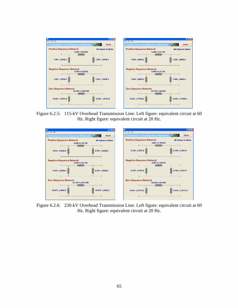
65

Figure 6.2.5: 115-kV Overhead Transmission Line: Left figure: equivalent circuit at 60

Hz. Right figure: equivalent circuit at 20 Hz.



66



6.2.2 Averaging Model: Converters

A method for modeling converters, which is named as averaging method, is presented in

this subsection. The averaging method is based on the steady-state analysis and the

equivalent relationship between input and output (two-port network analysis). In these

averaging concepts, the voltage and current ripples are averaged and harmonics at three-

phase side(s) are ignored. Note that the dynamic behaviors, such as switching operation

and transient phenomena, are not in consideration for the averaging converter models.

However, this method has the distinct advantages to quantitative analysis such as power

transfer capability, total operational losses, and optimal kV-level studies of networks.

Here, we develop three converters: a phase-controlled six-pulse converter, a phase-

controlled cycloconverter, and a PWM converter as shown in Figure 6.2.8. For averaging

models of the three converters, some assumptions are needed: (1) the voltages and

currents at the three-phase side(s) are assumed to be pure sinusoids and to be balanced, (2)

each converter is controlled by a specific control algorithm, and (3) inductance and

resistance are considered with approximate values. Note that the inductance is derived

from limiting current circuits and filter inductances and the resistance can be

approximated by the sum in electrical losses in snubber circuits, current limiting circuits,

and electrical switches.

67

V eajδ

E eajΦ

I eajθ

VKD

VAD

UKD

UAD

IKD

IAD

-jB

G(a)

V ea

jδ

E ea

jΦ

I ea

jθ

VKD

VAD

UKD

UAD

IKD

IAD

-jB

G

(b)

VaH e

IaH

jδ

ejθ

-jB

EaH ejφ

G

EaL ejγ

I aL ejβ

VaL ejα

(c)

Figure 6.2.8: Power Electronic Systems (a) Three-Phase, Six-Pulse Converter, (b)

Three-Phase, PWM Converter, and (c) Three-Phase, Six-Pulse Cycloconverter

The proposed averaging converters are modeled in the following details.

Six-pulse converter: The three-phase, six-pulse converter is based on an equidistant-

firing control. The firing pulses for thyristors are generated at equal intervals of 60o, and

all firings are delayed by equal delay angle α. In the control algorithm, the voltage

relationship can be denoted as follows:

cos23

LLdc vV or

cos23

LLdc vV , (6.2.6)

where VLL is the RMS value of the line-to-line voltage, Vdc is the DC-voltage, and γ is

extinction angle that used for the inverter mode of the six-pulse converter.

68

As seen in the equation above, the DC-voltage can be controlled by the combination of

the Line-to-Line voltage and the firing delay angle. Even though the DC-voltage or real

power of the six-pulse converter can be easily controlled by regulating the firing delay

angle, the reactive power cannot be controlled (but the imaginary power can be roughly

controlled by the combination of transformer’s tap control and firing angle control). That

is why the system needs FACTS devices to compensate the imaginary power at three-

phase lines.

PWM converter: The three-phase PWM converter is based on the Space-vector

modulation (SVM) control algorithm, since the converter connected to PCC is a grid side

converter (GSC). In this control algorithm, the voltage relationship can be presented by

the combinations of the modulation index (m) and the DC-voltage as follows:

mVV dcLL 2 (6.2.7)

where VLL is the RMS value of the line-to-line voltage, Vdc is the DC voltage, and m is

modulation index. Note the modulation index can be regulated between 0 and 1.

Here, we develop two control modes: a real-power and reactive-power control mode (PQ-

control mode) and a DC-voltage and reactive control mode (VQ-control mode).

Generally, the GSC is controlled by using the VQ-control mode, since the GSC has to

support the DC-voltage level at the PCC; and the stator-side converters (SSC) are

controlled by using the PQ-control mode, since the SSCs have to support maximum

power extraction from wind turbines. Also, the PWM converter has the controllability to

regulate reactive power at three-phase lines, which is the main difference from the six-

pulse converter.

Six-pulse cycloconverter: The three-phase, six-pulse cycloconverter in this technical

report is based on the two concepts: (1) The converter is operated in the circulating

current-free mode, and (2) the control algorithm is assumed to be the cosine-wave

crossing method. The cycloconverter model is more complicate compared to previous

models, since the reactive power at the both sides is not the same as the each other. So,

the power factor has to be computed using the relationship between the input current and

the output current. The relationship is denoted as follows:

oop Ir

I

cos2

36 (6.2.8)

n

n

o

oqnn

naII n

0

1

2 )12)(12(

2cos326 2

(6.2.9)

where Io is the RMS current at output, cosφo is the power factor at output, and r is the

modulation index that is computed as o

inputLL

outputa

V

Vr

30cos

.

69

The Ip and Iq are the in-phase current and the lagging quadrature current at the input side

of the cycloconverter, respectively. Using the two currents, the displacement factor at the

input can be computed as follows:

22cos

qp

p

i

II

I

(6.2.10)

where cosφi is the displacement factor at input.

The cycloconverter can control the voltage level and reactive power at output side by

regulating control references (voltage magnitude and phase angle at the output side).

However, the reactive power at the input side cannot be controlled and can be only

automatically regulated according to the modulation index and the displacement factor at

the output side. For example, while the modulation index is 1 and the displacement factor

at output is 1, the displacement angle at the input side is 34.5o. Note that the displacement

angle at input always exists between 34.5o and 145.5

o [44]. Since the cycloconverter

cannot control the imaginary power at input, the three-phase lines at input need a FACTS

device as the six-pulse converter.

6.3 Case Studies of Power-Transfer Capability

The study of the maximum power transfer capability is based on computer analysis. The

quantity of the power transfer is a scalar parameter which can be varied in the computer

model. The amount of transfer is gradually increased from the minimum quantity to the

maximum quantity of transfer power under operational constraints, and the maximum

quantity is recorded according to distances. Since the maximum power transfer capability

is the function of the operating voltage, the operating frequency, and the transmission

distances varying in the test systems shown in Figure 6.1.1: . The MPTC is recorded

according to these three parameters. For the studies, we present three cases based on three

different operating-voltages as shown in Table 6.3.1. Note that the operating voltages are

selected at 1/3 of nominal voltages of 115-kV, 230-kV, and 345-kV, since one of the

advantages by introducing LFAC transmission systems is that one can use the devices (of

the same V/H operating value) that have generally used in nominal frequency such as

transmission lines, transformers, and protection relays.

Table 6.3.1: Operating Voltages for Power Transfer Studies

Case 1 Case 2 Case 3

Operating Frequency

of 60Hz 38-kV 76-kV 115-kV

Operating Frequency

of 20Hz 38kV 76-kV 115-kV

70

To determine the maximum transmission capability, we checked the maximum

transmitted power from the PCC to the load center according to the transmission distance,

while the voltage drop between sending terminal and receiving terminal of the

transmission lines is remained between -5% and 5% of the operating voltage. Also, the

modulation indexes of converters are checked whether the converters are working in

reasonable limits of the modulation indexes (around 0.93-0.85). Since the inverter in the

LFAC systems have to support DC-voltage for the rectifiers which are connected to wind

turbines, the DC-voltage level is important for the reliable operation of the LFAC system.

Here, we present simulation results in tables and graphs representing the maximum

power transfer capability according to the distance from 10 to 200 miles.

Case 1: Rated Power Line Voltage: 38 kV (line-to-line).

Table 6.3.2: Maximum Transmission Capability at the Operation Voltage 38kV


Distance

(miles) 10 30 50 70 90 100 120 140 160 180 200

Transfer

Capability

(MW) at

60Hz

64.0 23.05 13.94 9.96 7.73 6.95 6.05 5.29 4.89 4.59 4.40

Transfer

Capability

(MW) at

20Hz

124.7 65.44 41.40 29.68 23.07 20.39 17.36 14.23 11.72 9.49 7.24

Figure 6.3.1: Power Transmission Capability of the Operation Voltage 38-kV

71




Distance

(miles) 10 30 50 70 90 100 120 140 160 180 200

Transfer

Capability

(MW) at

60Hz

180.3 82.8 57.54 44.17 36.78 34.31 30.56 27.98 26.19 24.84 23.38

Transfer

Capability

(MW) at

20Hz

225.3 141.3 106.1 86.28 73.49 68.29 60.19 54.27 49.22 45.21 41.96


72




Distance

(miles) 10 30 50 70 90 100 120 140 160 180 200

Transfer

Capability

(MW) at

60Hz

301.4 147.8 101.8 79.21 66.44 61.54 55.60 51.14 48.01 45.62 43.98

Transfer

Capability

(MW) at

20Hz

401.5 264.9 202.8 169.0 143.8 135.7 120.7 108.1 98.69 91.16 84.60


73

7 Transient Stability Studies

This section presents transient stability studies of alternative transmission systems using a

three-phase, six-pulse cycloconverter. Power systems are subjected to frequent

disturbances which might be small or large [44]. The small disturbances in LFAC

transmission systems should be the state variations of electrical switches, transformer tap

changes, load changes, etc. These small disturbances occur continuously and must be

managed appropriately in power systems for secure system operation. However, the large

disturbances, such as a short circuit on transmission systems and loss of a large generator,

result in fluctuation of system voltages, and eventually lead to sever damages to power

systems. The transient stability study in this section provides the ability of power systems

using LFAC transmission systems to maintain steady voltages from transient conditions.

7.1 Description and Technical Approach of Transient Stability Studies

Voltage stability and voltage recovery have been recognized to be of paramount

importance for secure system operation. As well-known, slow voltage recovery after

disturbance causes significant damages, in which voltage collapse and blackout can be

caused by power system instability, in power system [46]. Recently, power systems are

highly stressed with the interconnection of weak-synchronous wind systems, and a

knowledge and understanding of the impacts of the interconnected wind systems to

power system are forced for the reliable and secure operation of power system. In the past,

wind farms could be disconnected from power system during excessive voltage-

instability since the total capacity of wind-energy generation was small compared to that

of other sources. However, the penetration of wind energy in the grid is rapidly

increasing and the transmission capacity from wind farms may be a substantial portion of

the overall generation. So, the recent grid requirement demands continuing operation of

wind farm during and after contingencies [47]. Therefore, voltage-ride-through (VRT)

capability on wind-power systems is essential for stable operation of power system. The

VRT capability requirement on wind power systems are described by NERC standard.

Table 7.1.1 and Figure 7.1.1 provide voltage profiles which the wind-power systems

should sustain in the voltage requirement during system disturbances [48].

Table 7.1.1: NERC PRC-024-1 Voltage-Ride-Through Requirement

HVRT DURATION LVRT DURATION

Time

(second)

Voltage (pu) Time

(second)

Voltage (pu)

0.20 1.200 0.15 0.000

0.50 1.175 0.30 0.450

1.00 1.150 2.00 0.650

4.00 1.100 3.00 0.750

4.00 0.900

74

Figure 7.1.1: NERC PRC-024-1 Voltage-Ride-Through Requirement Curve

Note upper-limit is high-voltage-ride-through (HVRT) and the lower-limit is low-

voltage-ride-through (LVRT).

For the purpose of stability studies, a comprehensive modeling method is required.

Earlier attempts to model wind-generation systems were performed in steady state.

However, the excessive simplicity, in which the dynamics in power system are neglected,

leads erroneous assessment of system stability. So, a comprehensive modeling method is

required for the stability analysis. Here, we introduce a new approach to model power

devices composing the LFAC transmission systems. All models in power system are

modeled in quasi-steady state, but the modeling concepts are the similar to those in the

steady state. For example, the converters are modeled in averaging modeling concepts in

phasor representation; however, the continuous power flow and control constraints in

converters are allowed to vary in dynamics in each time step. Therefore, the power

systems modeled in quasi-steady state are desirable in voltage stability and voltage

recovery phenomena, while avoiding the either excessive modeling or simulation in full-

time domain. Note that the details are omitted in this subsection, since the modeling

processes in quasi-steady state are almost the same to those in steady state.

The methodology for stability study is based on computer simulations with case

configurations with LFAC transmission systems. While the LFAC transmission systems

are operating in steady state, a disturbance (fault) occur on a specific point, which might

be in wind farm, transmission systems, and grid systems. After the disturbance is cleared,

the case configurations are observed whether the case configurations can support

75

continuing operation over grid-cord requirement. Here we present two case-

configurations and some possible scenarios are made for the proposed case-studies.

7.2 Case Studies of Voltage-Stability Study

Here, we introduce two wind farm configurations for voltage-stability study as follows:

Configuration 1: A LFAC transmission system connecting 20 Hz series wind farm;

Configuration 2: Network fashion of a LFAC transmission connecting DC wind farm.

The two wind farm configurations are used for the simulation analyses of the voltage-

ride-through requirement. Each configuration is tested with its own scenarios according

to fault positions, disturbance type, and clearing time after a fault, etc.

Configuration 1: A LFAC transmission system connecting 20 Hz series wind farm

This configuration 1 presents an example of 20 Hz wind farm with a LFAC transmission

system connected to a power grid, as shown in Figure 7.2.1. The wind farm consists of

tens of wind-turbines and full-size inverters/converters. The each wind-turbine generates

5MW electrical power with 2.5-kV rating voltage and series connected to each other with

300-meter spacing. The distance of the LFAC transmission system is 25-mile with rating

voltage of 35-kV. At the point a cycloconverter converts the 20 Hz AC-power into 60 Hz

AC-power and step-up transformer boost the voltage to 115-kV, 60 Hz transmission at

that point.

Figure 7.2.1: Single-Line Diagram of a LFAC Transmission System Connecting a

Series LFAC Wind Farm to the Main Grid

76

Scenario 1: In this example study, the wind farm transmits 50-MW electrical power into

grid systems, a three-phase fault is generated at the remote grid (at the point of REMOT-

GRID in Figure 7.2.1), and the three-phase fault is cleared after 0.15 seconds from the

initial fault. The simulation results are represented in Figure 7.2.2. Note the three-phase

fault starts at 0.1 seconds and is cleared at 0.25 seconds. The graph (A) represents the

magnitude of phase-A voltage at the remote grid, and the graph (B) and the graph (C)

show the magnitude of phase-A voltage magnitude at the local gird and before the

cycloconverter, respectively. Note that the voltages are recovered and the frequency and

real-power are swing at equilibrium points as shown in Figure 7.2.3.

70.6

0.1

66.4

29.6

21.27

0.8

kV

kV

kV

35.4

48.0

14.64

0.00 0.66 1.32 1.98 2..67 3.33 4.00

(A)

(B)

(C)

Seconds

Figure 7.2.2: Configuration 1: Voltage Magnitude of Phase A at (A) Remote Grid

and (B) Local Grid, and (C) Before the Cycloconverter during a Three-Phase Fault

at Remote Grid

60.0

59.30

-117.4

-1.2

0.00 0.66 1.32 1.98 2.67 3.33 4.00

(A) Operating frequency at remote grid

(B) Real-power at remote gird

Hz

MW

Seconds

Figure 7.2.3: Configuration 1: (A) Operating Frequency and (B) Real Power at Remote

Grid during a Three-Phase Fault at Remote Grid

77

Scenario 2: The wind farm transmits 50-MW electrical power into grid systems in steady

state, and a three-phase breaker opens at 0.1 seconds and reclose at 0.25 seconds at PCC

of wind farm 1 (at the point of LFAC-FARM1 in Figure 7.2.1). The simulation results are

represented in Figure 7.2.4. The graph (A) represents the magnitude of phase-A voltage

at the remote grid, and the graph (B) and the graph (C) show the magnitude of phase-A

voltage magnitude at the local gird and before the cycloconverter, respectively. Note that

the voltages are in bound of the VRT requirement and the frequency and real-power are

swing at equilibrium points.

72.84

71.51

72.18

0.00 0.66 1.32 1.98 2.67 3.33 4.00

(A) Magnitude of phase-A voltage at remote grid

(B) Magnitude of phase-A voltage at local grid

kV

Seconds

(B) Magnitude of phase-A voltage before the cycloconverter

68.84

65.03

66.94kV

22.42

20.60

21.50kV

Figure 7.2.4: Configuration 1: Voltage Magnitude of Phase A at (A) Remote Grid,

(B) Local Grid, and (C) Before the Cycloconverter during the Recloser Operation

60.17

59.76

-114.1

-88.37

0.00 0.66 1.32 1.98 2.67 3.33 4.00



Hz

MW -101.2

Seconds


Grid during the Recloser Operation

Scenario 3: The wind farm transmits 50-MW electrical power into grid systems, a three-

phase fault is generated at the local grid (at the point of LOCAL-GRID in Figure 7.2.1),

78

and the three-phase fault is cleared after 0.15 seconds from the initial fault. The

simulation results are represented in Figure 7.2.6. When the three-phase fault generates at

local grid, the cycloconverter loses synchronism and the wind farm system is in

instability.

60.17

59.76

-114.1

-88.37

0.00 31.5 63.0 94.5 126.0 157.5 490

(A) Magnitude of phase-A before the cycloconverter

(B) Operating frequency before the cycloconverter

Hz

kV

-101.2

Milli-second

Figure 7.2.6: Configuration 1: (A) Voltage Magnitude of Phase A and (B) Operating

Frequency during the Three-Phase Fault at Local Grid

Configuration 2: A LFAC transmission system connecting 20 Hz series wind farm

This configuration 2 presents an example of series DC wind farm with network-fashion

of two LFAC-transmission systems connected to a power grid, as shown in Figure 7.2.7.

The wind farm consists of tens of wind-turbines in series DC-connection. The each wind-

turbine generates 5MW electrical power with 2.5-kV rating voltage and series connected

to each other with 300-meter spacing. The distance of the LFAC transmission system is

25-mile with rating voltage of 35-kV. At the point a cycloconverter converts the 20 Hz

AC-power into 60 Hz AC-power and step-up transformer boost the voltage to 115-kV, 60

Hz transmission at that point.

79

Figure 7.2.7: Single-Line Diagram of LFAC Transmission Network

Connecting a Series DC Wind Farm

Scenario 1: In this example study, the wind farm transmits 50-MW electrical power into

grid systems, a three-phase fault is generated at the remote grid (at the point of REMOT-

GRID in Figure 7.2.7), and the three-phase fault is cleared after 0.15 seconds from the

initial fault. The simulation results are represented in Figure 7.2.8. Note the three-phase

fault starts at 0.1 seconds and is cleared at 0.25 seconds. As shown in Figure 7.2.8, the

graphs (A) represent the magnitude of phase-A voltage at the remote grid, and the graph

(B) and the graph (C) show the magnitude of phase-A voltage magnitude at the local gird

1 and before the cycloconverter, respectively. Note that the voltages are recovered and

the frequency and real-power are swing at equilibrium points as shown in Figure 7.2.9.

Since the VRT requirement is satisfied, the configuration 2 is stable with three-phase

fault at remote grid.

80

70.6

0.1

66.4

29.6

21.27

0.8

kV

kV

kV

35.4

48.0

14.64

0.00 0.66 1.32 1.98 2.67 3.33 4.00


(B) Magnitude of phase-A voltage at local grid-1

(C) Magnitude of phase-A voltage before the cycloconverter

Seconds

Figure 7.2.8: Configuration 2: Voltage Magnitude of Phase A (A) at Remote Grid, (B)

at Local Grid 1, and (C) Before the Cycloconverter during a Three-Phase Fault at Remote

Grid

60.0

58.13

-276.7

80.1

0.00 0.67 1.33 1.99 2.66 3.33 4.00



Hz

MW -98.3

Seconds


Grid during a Three-Phase Fault at Remote Grid

Scenario 2: The wind farm transmit 50-MW electrical power into grid systems, a three-

phase fault is generated at the local-grid 1 (at the point of LOCAL-GRID-1 in Figure

7.2.7), and the three-phase fault is cleared after 0.15 seconds from the initial fault. The

simulation results are represented in Figure 7.2.8. Note the three-phase fault starts at 0.1

seconds and is cleared at 0.25 seconds. As shown in Figure 7.2.10, the graphs (A) and (B)

represent the magnitude of phase-A voltage at the remote grid and at local grid 1, the

graphs (C) and (D) are the real-power and operating frequency at remote grid. Note that

the voltages are recovered and the frequency and real-power are swing at equilibrium

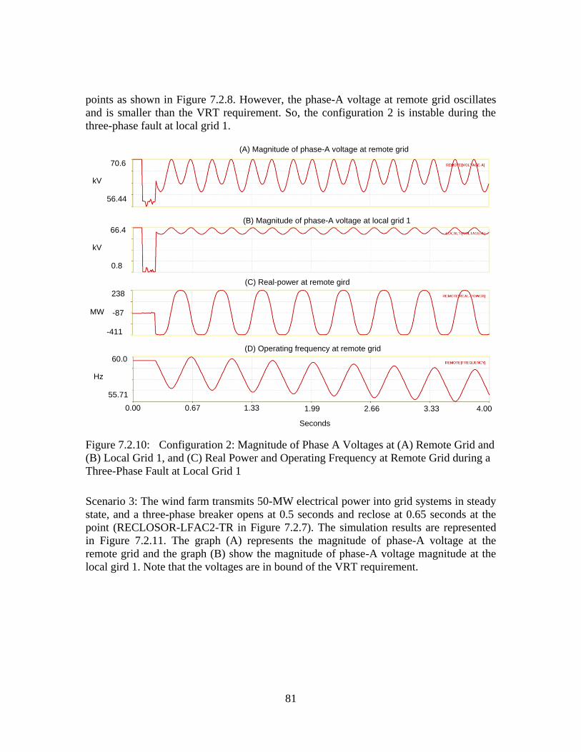
81

points as shown in Figure 7.2.8. However, the phase-A voltage at remote grid oscillates

and is smaller than the VRT requirement. So, the configuration 2 is instable during the

three-phase fault at local grid 1.

60.0

55.71

-411

238

0.00 0.67 1.33 1.99 2.66 3.33 4.00

(D) Operating frequency at remote grid

(C) Real-power at remote gird

Hz

MW -87

(B) Magnitude of phase-A voltage at local grid 1


66.4

0.8

kV

70.6

56.44

kV

Seconds

Figure 7.2.10: Configuration 2: Magnitude of Phase A Voltages at (A) Remote Grid and

(B) Local Grid 1, and (C) Real Power and Operating Frequency at Remote Grid during a

Three-Phase Fault at Local Grid 1


state, and a three-phase breaker opens at 0.5 seconds and reclose at 0.65 seconds at the

point (RECLOSOR-LFAC2-TR in Figure 7.2.7). The simulation results are represented

in Figure 7.2.11. The graph (A) represents the magnitude of phase-A voltage at the

remote grid and the graph (B) show the magnitude of phase-A voltage magnitude at the

local gird 1. Note that the voltages are in bound of the VRT requirement.

82

70.8

70.0

63.2

67.7

0.00 0.66 1.32 1.98 2.67 3.33 4.00



kV

kV

Seconds

Figure 7.2.11: Configuration 2: Magnitude of Phase A voltages at (A) Remote Grid and

(B) Local Grid 1 during Recloser Operation at RECLOSOR-LFAC2-TR


state, and a three-phase breaker opens at 0.5 seconds and reclose at 0.65 seconds at the

point (RECLOSOR-LFAC1-TR in Figure 7.2.7). That is, the wind farms and local-grid 2

are disconnected from the main grid. The simulation results are represented in Figure

7.2.12. The graph (A) represents the magnitude of phase-A voltage at the remote grid,

and the graph (B) show the magnitude of phase-A voltage magnitude at the local gird 1.

Note that since the phase-A voltage at local-grid 1 is not satisfied by the VRT

requirement, the configuration 2 is instable while the main-grid is disconnected from the

wind farms and local-grid 2.

70.8

70.6

66.4

67.5

0.00 0.66 1.32 1.98 2.67 3.33 4.00



Hz

kV

Seconds

Figure 7.2.12: Configuration 2: Magnitude of Phase A Voltages at (A) Remote Grid and

(B) Local Grid 1 during Recloser Operation at RECLOSOR-LFAC1-TR

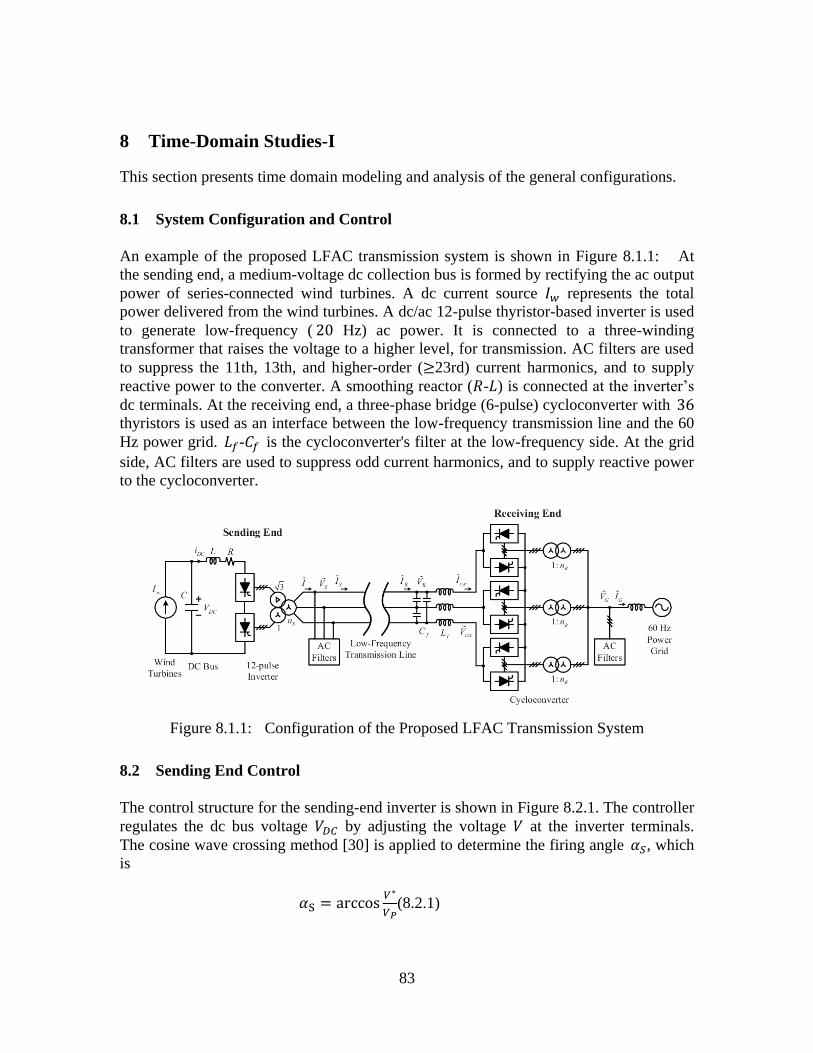
83

8 Time-Domain Studies-I

This section presents time domain modeling and analysis of the general configurations.

8.1 System Configuration and Control

An example of the proposed LFAC transmission system is shown in Figure 8.1.1: At

the sending end, a medium-voltage dc collection bus is formed by rectifying the ac output

power of series-connected wind turbines. A dc current source represents the total

power delivered from the wind turbines. A dc/ac 12-pulse thyristor-based inverter is used

to generate low-frequency ( Hz) ac power. It is connected to a three-winding

transformer that raises the voltage to a higher level, for transmission. AC filters are used

to suppress the 11th, 13th, and higher-order ( 23rd) current harmonics, and to supply

reactive power to the converter. A smoothing reactor ( - ) is connected at the inverter’s

dc terminals. At the receiving end, a three-phase bridge (6-pulse) cycloconverter with

thyristors is used as an interface between the low-frequency transmission line and the 60

Hz power grid. - is the cycloconverter's filter at the low-frequency side. At the grid

side, AC filters are used to suppress odd current harmonics, and to supply reactive power

to the cycloconverter.

Figure 8.1.1: Configuration of the Proposed LFAC Transmission System

8.2 Sending End Control

The control structure for the sending-end inverter is shown in Figure 8.2.1. The controller

regulates the dc bus voltage by adjusting the voltage at the inverter terminals.

The cosine wave crossing method [30] is applied to determine the firing angle , which

is

(8.2.1)

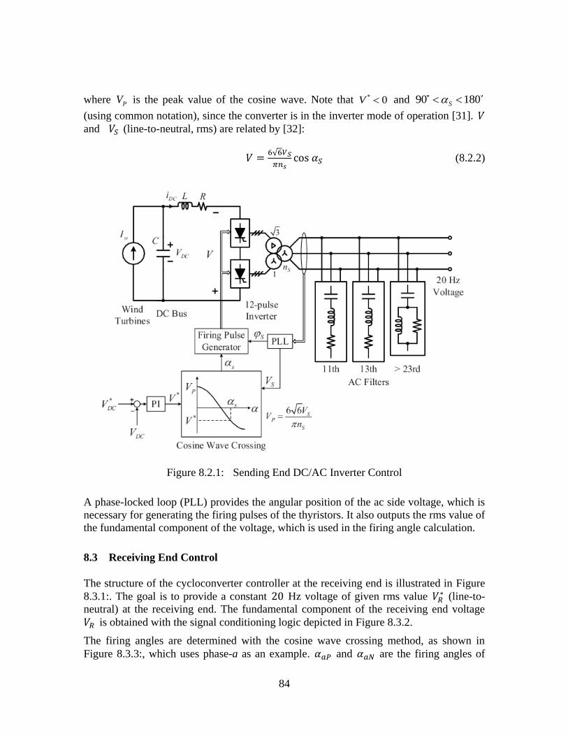
84

where PV is the peak value of the cosine wave. Note that * 0V and 90 180S

(using common notation), since the converter is in the inverter mode of operation [31].

and (line-to-neutral, rms) are related by [32]:

√

(8.2.2)

Figure 8.2.1: Sending End DC/AC Inverter Control

A phase-locked loop (PLL) provides the angular position of the ac side voltage, which is

necessary for generating the firing pulses of the thyristors. It also outputs the rms value of

the fundamental component of the voltage, which is used in the firing angle calculation.

8.3 Receiving End Control

The structure of the cycloconverter controller at the receiving end is illustrated in Figure

8.3.1:. The goal is to provide a constant Hz voltage of given rms value (line-to-

neutral) at the receiving end. The fundamental component of the receiving end voltage

is obtained with the signal conditioning logic depicted in Figure 8.3.2.

The firing angles are determined with the cosine wave crossing method, as shown in

Figure 8.3.3:, which uses phase-a as an example. and are the firing angles of

85

the phase-a positive and negative converter, respectively (denoted as ‘aP’ and ‘aN’ in

Figure 8.3.1:). For the positive converter, the average voltage at the 20 Hz terminals is

given by [32]:

√

(8.3.1)

where is the rms value of the line-to-neutral voltage at the grid side, and is the

turns ratio of the transformers. The condition ensures that average

voltages with the same polarity are generated from the positive and negative converter at

the 20 Hz terminals [34]. However, the firing pulses and are not simultaneously

applied to both converters, in order to obtain a non-circulating current mode of operation.

This functionality is embedded in the ‘Bank Selector’ block of Figure 8.3.1:, which

operates based on the filtered current ̂ . Note (for later use) that the maximum line-

to-neutral rms value of the 20 Hz cycloconverter voltage is [30]:

√

(8.3.2)

and that a voltage ratio is defined as

(8.3.3)

In practice, the theoretical maximum value cannot be achieved, due to the f m ’ u y

86

Figure 8.3.1: Receiving End Cycloconverter Control (The reference frame

transformation matrix is defined in [33], and transforms variables from the

stationary to the synchronous reference frame.)

Figure 8.3.2: Details of the Signal Conditioning Block(LPF = low-pass filter; the time

constants are s and s for the voltage and current respectively.)

87

Figure 8.3.3: Modulator for Phase A

8.4 System Design

8.4.1 Main Power Components

The main power components are selected based on a steady-state analysis of the LFAC

transmission system shown in Figure 8.1.1: under the following assumptions:

Only fundamental components of voltages and currents are considered. The

receiving end is modeled as a 20 Hz voltage source of nominal magnitude.

The power losses of the reactor, thyristors, filters, and transformers are ignored.

The resistances and leakage inductances of transformers are neglected.

The AC filters are represented by an equivalent capacitance corresponding to the

fundamental frequency.

The design is based on rated operating conditions (i.e., maximum power output).

At the steady state, the average value of the DC current is equal to , so the power

delivered from the wind turbines is

(8.4.1)

For the 12-pulse converter, the rms value of the current at the transmission side is [32]:

88

√

√

(8.4.2)

Hence, (8.4.2) can be written as

(8.4.3)

with

√

(8.4.4)

Let ̃ and ̃ denote phasors of the line-to-neutral voltage and line current,

respectively. Since ̃ lags ̃ by [32], it follows that ̃ . So, the

active power delivered by the 12-pulse inverter is given by

(8.4.5)

Substitution of (8.4.3) into (8.4.5) yields

(8.4.6)

and

√

(8.4.7)

The reactive power generated from the 12-pulse inverter is

(8.4.8)

From (8.4.5)–(8.4.8), it follows that

√ (8.4.9)

The negative sign in (8.4.8) and (8.4.9) indicates that the 12-pulse inverter always

absorbs reactive power. Equation (8.4.9) shows that can be expressed as a function

. Based on the above analysis, the steady-state single-phase equivalent

89

circuit of the LFAC transmission system is shown in Figure 8.4.1:. is the equivalent

capacitance of the sending-end AC filters at fundamental frequency. The transmission

line is modeled by a -equivalent (positive-sequence) circuit using lumped parameters.

The well-known hyperbolic trigonometric expressions for and

are used [35].

Given a power rating of a wind power plant , the maximum reactive power that is

absorbed by the 12-pulse inverter can be estimated according to (8.4.9), which yields

√ (8.4.10)

where is the nominal transmission voltage level (line-to-line rms). Here, it is assumed

that the sending-end AC filters supply the rated reactive power to the inverter. Therefore,

(8.4.11)

where rad/s. In addition, the apparent power rating of the transformer at the

sending end should satisfy

√

√ (8.4.12)

At the 60 Hz grid side, the reactive power capacity of the AC filters and the apparent

power rating of the transformers depend on the cycloconverter’s voltage ratio , which is

a design parameter, and the 20 Hz side power factor [34], which can be estimated as

follows.

For a given transmission cable, the voltage ratings (nominal and maximum voltage), the

current rating, and the distributed cable parameters (resistance, inductance, and

capacitance per unit length) are known. Here, it is assumed that a power cable is chosen

to transmit the rated wind power plant power without violating the cable’s voltage

and current ratings. (The relationship between active power through the cable and

maximum transmission distance, given a certain cable, will be discussed later.) For

simplicity, it is further assumed that the rms value of line-to-line voltage at both sending

and receiving ends is and the current through and is approximately equal to the

current rating of the cable .

Since the AC filters are designed to supply all reactive power to the 12-pulse inverter at

the sending end, the reactive power injected into the cycloconverter’s 20 Hz side can be

estimated using

m{ }

m{ }

(8.4.13)

90

where the first two terms represent the reactive power generated from the cable and the

filter’s capacitor, and the last two terms represent the reactive power consumed by

the cable and the filter’s inductor. The active power injected into the cycloconverter

from the 20 Hz side can be estimated using

{ }

{ } (8.4.14)

where the last two terms represent the power loss of the cable. Thus, the 20 Hz side

power factor can be estimated according to (8.4.13) and (8.4.14).

Now the 60 Hz side power factor at the transformers’ grid-side terminals can be

obtained using the method presented in [34]. Then the apparent power rating of each out

of the three receiving-end transformers should satisfy

(8.4.15)

Also, it is assumed that the grid-side AC filters are designed to supply the rated amount

of reactive power to the cycloconverter.

Figure 8.4.1: Equivalent Circuit of 20 Hz Transmission System

Figure 8.4.2: Equivalent Circuit of 20 Hz Transmission System for Harmonic Analysis

91

8.4.2 Filter Design

At the sending end, the 12-pulse inverter produces harmonics of order ,

, and can be represented as a source of harmonic currents ( in Figure

8.4.2:). These current harmonics are filtered by two single-tuned filters for the 11th and

13th harmonics, and one damped filter for higher-order harmonics ( 23rd). Generally,

the filter design is dependent on the reactive power that the filter supplies at fundamental

frequency (also known as the filter size) and the required quality factor [36]. The total

reactive power requirement of these filters can be estimated based on (8.4.10). Here, it is

assumed that the total reactive power requirement is divided equally among the three

filters. The quality factor for each filter can be determined using the method presented

in 36. A high quality factor ( ) is used for the single-tuned filters, and a low

quality factor ( ) is used for the high-pass damped filter. Finally, with the

capacitance and quality factor known, the inductance and resistance of each filter can be

determined. With such filter design, the 12-pulse-related current harmonics originating at

the sending end are essentially absent from the transmission line.

At the receiving end, there are two groups of filters which include the AC filters at the 60

Hz side and the filter at the 20 Hz side. At the 60 Hz side, if the cycloconverter

generates exactly Hz, it can be shown [34] that the line current has only odd

harmonic components, i.e., 3rd, 5th, 7th, . Here, three single-tuned filters and one

damped filter are used to prevent these harmonic currents from being injected into the 60

Hz power grid. These filters are designed with a procedure similar to that for the ac filters

at the sending end.

At the 20 Hz side, the line-to-neutral voltage has harmonics of order [34].

However, the harmonic components of order equal to integer multiples of three are absent

in the line-to-line voltage. Therefore, as seen from the 20 Hz side, the cycloconverter acts

as a source of harmonic voltages of orders (

in Figure

8.4.2:). The design of the filter has two objectives:

1) to decrease the amplitudes of the voltage harmonics generated by the

cycloconverter;

2) to increase the equivalent harmonic impedance magnitudes seen from the

receiving end, indicated by in Figure 8.4.2:.

The design procedure presented here takes into account the voltage harmonics of order 5,

7, 11, and 13. For cycloconverters, the amplitude of the voltage harmonics only depends

on the voltage ratio and the fundamental power factor at the 20 Hz side, under the

assumption of sinusoidal output current [34], which is sufficient for design purposes.

Generally, the voltage harmonics tend to become worse with decreasing . Here, we set

. Figure 8.4.3: illustrates the relationship between the per unit amplitudes of the

voltage harmonics under consideration (5th, 7th, 11th, and 13th) and the power factor

angle , computed based on formulas in [34]. Apparently, for the 5th and 7th voltage

harmonics, the amplitudes are symmetric with respect to , and positive (i.e.,

reactive power consumption by the cycloconverter) can result in reduced amplitudes of

92

the 11th and 13th voltage harmonics. At , minimum amplitudes are obtained.

However, this value is unacceptably low, so is selected (for operation at rated

power). After has been determined, it follows from (8.4.13) and (8.4.14) that there is a

linear relation between and , as in , since

.

However, any ( , ) pair determined based on this equation should only be used as an

initial guess. These initial parameters might not yield the required power factor angle

( ) due to the simplifying assumptions made in the analysis. The proper filter

parameters can be obtained by solving the circuit shown in Figure 8.4.1:1. For example,

given a value for , the capacitance that leads to the right power factor angle can be

found by searching around its initial guess value. Therefore, if varies within a certain

range, a number of ( , ) pairs can be obtained. Among these ( , ) candidates, a

selection is made such that the magnitudes for are deemed to

be adequately large. A numerical example will be provided in the next section.

Figure 8.4.3: Harmonic Voltage Amplitudes Generated by the Cycloconverter

at the 20 Hz Side

8.5 Case Study

In this section, a design case study of a 20 Hz LFAC transmission system is presented.

The transmission voltage level is chosen as kV. An appropriate submarine three-

core XLPE power cable is selected (nominal voltage: kV, maximum voltage:

kV, rated current: 825 A, cross section: mm , copper conductor). The cable’s

1The circuit can be solved by formulating this as a three-bus power flow problem, where the sending end is

a PQ-type bus. Since , the power flow is solved for a range of

values, until the

computed provides the correct value of , when substituted in .

93

resistance, inductance, and capacitance per km are m /km, mH/km, and

F/km, respectively [37, 38].

The LFAC system is compared to a conventional 60 Hz HVAC transmission system that

uses the same power cable, with a steady-state single-phase equivalent circuit shown in

Figure 8.5.1:. represents the short-circuit level of the 60 Hz power grid. Shunt

reactive compensation ( and in Fig. 2) is connected at both ends to improve the

active power transmission capability, especially for long transmission distances [39]. The

power grid voltage is kV line-to-line. The short-circuit level is MVA,

which is a typical value for a -kV system 40. At the sending end, unity power factor

is assumed ( ), in order to calculate the maximum possible transmissible active

power through the cable. Two cases are considered:

1) No shunt reactive compensation, i.e., . This case is denoted as ‘60

Hz ’.

2) Shunt reactive compensation split equally between the two ends. This case is

denoted as ‘60 Hz ’. The total amount of reactive compensation is

m{ } , so

.

Figure 8.5.1: Equivalent Circuit of 60 Hz Transmission System

The relationship between sending end active power and maximum transmission

distance is calculated using the circuit of Figure 8.5.1:, and plotted in Figure 8.5.2:. The

maximum transmission distance is obtained whenever the current or the voltage rating of

the power cable is reached. In this case study, the cable’s rated apparent power is 188

MVA. The maximum distance for transmitting 180 MW is 45 km without shunt

compensation, and 70 km with shunt compensation.

The 20 Hz LFAC system is designed to transmit MW over km. At the sending

end, the DC bus voltage level is chosen as kV. A 214-MVA, kV ( ), 20 Hz phase-shift transformer is used. With the 20 Hz rated frequency, this

transformer would have larger volume compared to 60 Hz transformers. This is a

drawback of the proposed LFAC system. The total size of the AC filters at the sending

end is MVAr.

94

Figure 8.5.2: Sending End Active Power vs. Max. Transmission Distance

For the cycloconverter, the voltage (line-to-line) generated at the 20 Hz side is kV.

The voltage ratio is selected as , and the 20 Hz side power factor angle is

designed to be . According to (8.3.2) and (8.3.4), the transformer ratio is

, and the 60 Hz side power factor is [34]. Based on the analysis of

Section 8.2.1 and equation (8.4.15), the apparent power rating of each cycloconverter

transformer is chosen to be MVA. The total size of AC filters at the 60 Hz side is

MVAr.

Figure 8.5.3: depicts the approximate linear relation between and by a dashed

line. The more accurate capacitance values that yield the required power factor angle are

represented by the solid curve. A solution is found for between mH and mH.

Note that a solution can be obtained for outside this range as well; however, in this

case, either the current or the voltage rating of the power cable are violated. Figure 8.5.4:

shows the variation of corresponding to the feasible ( , ) pairs. It can be

seen that the filter with mH and F gives the maximum

impedance magnitudes for the 5th, 11th, and 13th harmonics.

95

Figure 8.5.3: Filter Design

Finally, based on the above system parameters, the relationship between sending-end

active power and maximum transmission distance for the 20 Hz LFAC system is

calculated and superimposed in Figure 8.5.2. It can be observed that the proposed LFAC

system is a feasible option for delivering the rated power over a distance ca. 2-3 times

further than the HVAC solution. Typically, for distances longer than 100 km, HVDC

systems are the preferred solution 41, but an LFAC system could be an alternative

transmission technology for the 100-200 km range, at least from a technical standpoint.

Figure 8.5.4: Equivalent Impedance Magnitude Seen from the Receiving End

( )

8.6 Simulation Results

To demonstrate the validity of the proposed LFAC system, simulations have been carried

out using Matlab/Simulink and the Piecewise Linear Electrical Circuit Simulation

(PLECS) toolbox. The wind power plant is rated at MW, and the transmission

distance is km. The system parameters are listed in Table 8.6.1:. The parameters of

96

the PI controllers in Figure 8.2.1: and Figure 8.3.1: are listed in Table 8.6.2. The

transmission power cable is modeled by cascading identical sections.

Table 8.6.1: LFAC System Simulation Parameters

Sending End

DC Bus Capacitor F

Smoothing Inductor H, m

20 Hz Phase-shift Transformer

Rated Power MVA Voltage kV

Winding

Resistance

p.u. Leakage

Reactance

p.u.

Magnetizing

Resistance

p.u. Magnetizing

Reactance

p.u.

AC Filters ( MVAr, kV, Hz)

R ( ) L (mH) C ( F)

th

th

rd

Transmission Power Cable (132 kV)

Resistance m /km Inductance mH/km

Capacitance F/km Rated Current A

Receiving End

Filter mH, F

Transformers

Rated Power MVA Voltage kV

Winding

Resistance

p.u. Leakage

Reactance

p.u.

Magnetizing

Resistance

p.u. Magnetizing

Reactance

p.u.

AC Filters ( MVAr, kV, Hz)

R ( ) L (mH) C ( F)

rd

th

th

th

97

Table 8.6.2: Parameters of PI Controllers with Transfer Function

Sending

end

Receiving

end

1 0.125

0.4 0.05

Figure 8.6.1: shows the steady-state line-to-line voltage and current waveforms at the

sending end, the receiving end, the 20 Hz side of the cycloconverter, and the 60 Hz

power grid side under rated power conditions. The 20 Hz voltage generated from the

cycloconverter has significant harmonic distortion (THD is ). Due to the filter,

the voltages at the receiving end and the sending end have reduced THD values (

and , respectively). The measured fundamental power factor angle at the 20 Hz

side of the cycloconverter is , which is close to the design requirement.

Figure 8.6.2: depicts the results of a transient simulation where the power from wind

turbines ramps from 170 MW to 180 MW, at 10 MW/s. Shown are the transient

responses of the active power injected into the 60 Hz power grid, the DC bus voltage at

the sending end, and the magnitude of the fundamental component of the 20 Hz voltage

at the receiving end.

Sending end b) Receiving end

Cycloconverter 20 Hz side d) 60 Hz power grid side

Figure 8.6.1: Simulated Voltage and Current Waveforms

98

Figure 8.6.2: Transient Waveforms

8.7 Conclusion

A low-frequency AC transmission system has been proposed. The methodology to design

the system’s components and control strategies has been discussed. The use of low

frequency can improve the transmission capability of submarine power cables due to low

cable charging current. The proposed LFAC system appears to be a feasible solution for

the integration of offshore wind power plants over long distances. Technically, it could

be used to substitute HVDC systems. Furthermore, it is easier to establish a low-

frequency AC network to transmit bulk power from multiple plants.

In order to help the wind energy industry to make a better-informed decision for the

transmission type for offshore wind power, it is of significance to perform a complete

technical and economic comparison among HVAC, HVDC, and LFAC, e.g., transmission

efficiency, transient stability, and investment evaluation. The above are subjects of

ongoing work.

99

9 Time-Domain Studies-II

This section presents time-domain studies of alternative-transmission systems using a

three-phase, six-pulse cycloconverter. Time-domain simulation is utilized for better

understanding of the dynamic behavior of the alternative transmission systems.

Alternative-transmission systems employ phase-controlled converters and PWM

converters, and the converters using electrical switches are well-known harmonic sources.

Harmonic pollution in power system causes several problems: heat problem in

transformer and electrical machines, aging problem of isolation of power-system devices,

malfunction of dynamic-control systems, and inductive interference over communication

networks. Harmonics should be mitigated in power systems and the voltages and currents

at every point should be near pure sine-waves; the harmonics should be within allowable

limits. So, understanding the harmonic content from alternative systems is necessary to

design the harmonic filters for the alternative-transmission systems for high power

quality.

Since power consumption from electrical load varies in real time, the flexible control of

an amount of the transfer power from wind farms can allow continuing operation of

electrical systems. Since the alternative-transmission systems consist of several

converters, operating voltage, operating frequency, and real- and reactive-power can be

controlled by changing their control references. However, inappropriate control algorithm

or control parameters become the direct reason of switching malfunctions. Eventually,

the voltage spikes and current spikes can occur and the electrical switches should be

damaged physically. Power-transient studies can allow the optimal design of control

systems of alternative transmissions and the knowledge to support continuing operation

of the LFAC transmission systems.

9.1 Technical Approach of Time-Domain Studies

The time-domain studies are performed using two LFAC-transmission systems

interconnecting a wind farm and grid systems as shown in Figure 9.1.1 and Figure 9.1.2.

For the LFAC-transmission systems, variable-speed wind-turbine systems (type-3 and

type-4 wind generation units) are considered, since variable-speed wind-generation

systems are attractive for increasing energy capture and reducing mechanical-fatigue

damage. The variable-speed wind-turbine systems cannot be directly connected to grid

systems and converters are used to connect systems with different frequency. In the

proposed wind farm configurations, three-phase PWM converters and a three-phase six-

pulse cycloconverter are used to interconnect systems with different frequency. The

three-phase PWM converters interconnect wind farms and a LFAC transmission system

while the three-phase cycloconverter interconnect the LFAC transmission system and

nominal-frequency grid systems. Also, each converter performs its own roles: the

cycloconverter controls operating frequency at the LFAC transmission system and allows

voltage synchronization for the three-phase PWM inverters; the three-phase PWM

inverters should support DC-voltage level and the controllability of reactive power of the

100

LFAC transmission systems; and the three-phase PWM rectifiers allow the power

tracking to extract maximum power from wind turbines.

WTG

WTG

WTG

G

G

Remote Wind

Farm

20Hz

tranmsission

60Hz,

main grids

Cycloconverter

station

PCC

Figure 9.1.1: Wind Farm Configuration: LFAC Wind Farm and LFAC Transmission

WTG

WTG

WTG

G

G

Remote Wind

Farm

20Hz

tranmsission

60Hz,

main grids

Cycloconverter

station

AC/DC DC/AC

Figure 9.1.2: Wind Farm Configuration: Series DC Wind Farm and LFAC Transmission

For the realistic models of the wind farm configurations, each device (containing the

LFAC transmission systems) has to be modeled in realistic manners. For the purpose, we

use quadratic integration method and Kirchhoff’s current low. Since mathematical

models of physical components in power systems are generally modeled by state

equations, these equations cannot be solved exactly in explicit calculations. So,

approximate methods are necessary to model power systems and the quadratic integration

method is introduced as the approximate method. As soon as all devices are model, the

devices are merged to form an entire network system using Kirchhoff’s current law. More

details are presented in next subsection.

Using the realistic network systems, power-transient studies and harmonics studies are

performed. For the power-transient study, power step changes (the required power-order)

101

suddenly occur while the LFAC transmission systems are operating in steady state. Also,

harmonics studies are performed according to the control modes (partial- and full-

circulating current modes) and modulation indexes of the cycloconverter. Since the

cycloconverter is directly connected to grid systems, we present harmonic contents of

voltages and currents before and after the cycloconverter.

9.2 Methodology for Simulation Models in Time-Domain

Time-domain studies are based on computer analysis in time-domain. For the purpose,

the reliable and realistic models for alternative transmission systems connecting wind

farms are needed. Here, we introduce an advanced time-domain method, which is named

as quadratic-integration method. The quadratic integration has demonstrated the superior

properties compared to pre-dominant methods (such as backward Euler’s method and

trapezoidal integration method). Especially, the quadratic integration is a powerful

simulation method for nonlinearities and switching systems, since the method is totally

free from artificial numerical oscillations that are not natural phenomena from systems

instability but fictitious phenomena from simulation methods themselves. The basic

concepts and advantages of the quadratic integration are in Appendix C.

The detailed modeling methodology of time-domain models is presented based on the

application of the quadratic integration method and standard nodal analysis. The

modeling process for time-domain models is performed: (1) each component constructing

a power device is written in state equations, (2) the quadratic integration is applied to the

state equations to derive the algebraic-companion form (ACF) of the each component,

and (3) the ACF of the power device is constructed by merging the ACF of all

components in the power device. With the modeling process above, power devices

composing alternative-transmission systems are modeled. Here we present a three-phase

transformer model, a three-phase, six-pulse, cycloconverter, and a three-phase PWM

converter, since the models are essential for the alternative transmission systems.

9.2.1 Three-Phase Transformer

Modeling of the three-phase isolation transformer can be modeled using three single-

phase transformers. First, a single-phase transformer is written as state equations and the

quadratic integration method is applied to the state equations for algebraic-companion

forms. Finally, the algebraic companion forms are interconnected to provide the topology

of the three-phase transformer. Here, we only introduce a wye-delta connected three-

phase transformer, even though all the combinations of connections can be modeled.

Figure 9.2.1 shows (A) the three-phase isolation transformer, and (B) a single-phase

transformer.

102

(A)

r1 L1

rc Lm

r2 L2

r1 L1

rc Lm

r2 L2

r1 L1

rc Lm

r2 L2

0

(22)

1

(23)

2

(24)

3

(25)

4

(26)

5

(27)

6

(28)

7-11

(29-33)

12-16

(34-38)

17-21

(39-43)

(B)

)(1 tV

)(2 tV

)(3 tV

)(4 tV

)(1 ti

)(2 ti

)(3 ti

)(4 ti

1r 1L2r 2L

cr mL

)(tim

)(te )(tetn

1

2

3

4-8

Figure 9.2.1: (A) Three-Phase Y-Δ Isolation Transformer

and (B) Single Phase Transformer

The differential equations and algebraic equations describing the single-phase

transformer model are written in state-space form. There are two sets of equations:

external equations and internal equations. The external equations consist of the node

currents of the single phase transformer and the internal equations are derived with

internal states. The state-space model is given as follows:

)()( 11 titi L (9.2.1)

)()( 12 titi L (9.2.2)

)()( 33 titi L (9.2.3)

)()( 34 titi L (9.2.4)

103

)()()()(0 31 tetirtitrtir mcLcLc (9.2.5)

)()(0 ttiL mm (9.2.6)

)()()()()(0 111121 tidt

dLtirtetvtv LL (9.2.7)

)()()()()(0 323243 tidt

dLtirtettvtv LL (9.2.8)

)()(0 tdt

dte (9.2.9)

where λ is magnetic flux linkage.

The compact matrix form is also given as follows:

)()()( tVdt

dNtVMtI

(9.2.10)

where:

000100000

0001100

00100011

00100000

010000100000000

100000000010000000010000000

2

1

rt

r

L

trrr

M

m

ccc

,

001000000

00000000

00000000000000000000000000000000000000000000000000000000000000

2

1

L

L

N

TtititititI 00000)()()()()( 4321

,

TLLm titittetitvtvtvtvtV )()()()()()()()()()( 314321

The compact matrix form of the single-phase transformer is reformulated into algebraic-

companion form applying quadratic integration. The transformer algebraic-companion

form (ACF) at each time step [t-h, t] is:

)()()(

)(

)(

)(htIDhtVC

tV

tVB

tI

tIA

mm

(9.2.11)

104

where:

ss

ss

Ah

Ah

Ah

Ah

A

3

2

6

324,

Mh

NMh

NMh

Mh

B

3

2

6

324,

NMh

NMh

C

6

24

5,

s

s

Ah

Ah

D

6

24

5,

Tmmmmm tititititI 00000)()()()()( 4321

,

TmLmLmmmmmmmmm titittetitvtvtvtvtV )()()()()()()()()()( 314321

,

As=diag(1, 1, 1, 1, 0, 0, 0, 0, 0), and tm is the mid-point of the integration time step.

The algebraic-companion forms of the three single-phase transformers are merged to

form the algebraic companion form of a three-phase isolation transformer. For this

purpose it is noted that each single-phase transformer is connected to specific nodes of

the three-phase isolation transformer. The connectivity of each single-phase transformer

is defined in terms of the order of the corresponding states. Figure 9.2.1 shows the node

numbers on specific nodes. Table 9.2.1 provides the connectivity pointers of the single

phase transformers. The merging of these models into an overall model of the three-phase

transformer is achieved by writing the Kirchhoff’s current law at each internal node of

the three-phase transformer substituting the appropriate equations. This process is

achieved with the algorithm below:

DO WHILE ( itrans Number of 1-Φ transformers)

DO WHILE ( i < Number of ROW1-Φ)

1i = Valve Pointer [ i ][ itrans ]

DO WHILE ( j < Number of Column1-Φ)

1j = Valve Pointer [ j ][ itrans ]

]][[]1][1[ 13 jiAjiA

]][[]1][1[ 13 jiBjiB

]][[]1][1[ 13 jiCjiC

]][[]1][1[ 13 jiDjiD

END DO

END DO

END DO

105

where ,...,,2,1 matrixeachofrowofnumberi

matrixeachofcolumnofnumberj ...,,2,1 , and

strnsformerofnumberitrans 1....,,2,1 .

Table 9.2.1: Connectivity Pointer of Three Single-Phase Transformers

# 1-Φ

transformer Connective Node in the Three-phase Transformer

1 t 0 3 4 6 7 8 9 10 11

tm 22 25 26 28 29 30 31 32 33

2 t 1 3 5 4 12 13 14 15 16

tm 23 25 27 26 34 35 36 37 38

3 t 2 3 6 5 17 18 19 20 21

tm 24 25 28 27 39 40 41 42 43

The end result is the algebraic-companion form of the overall three-phase transformer

given by the following equation:

)()()(

)(

)(

)(3333 htIDhtVC

tV

tVB

tI

tIA

mm

(9.2.12)

where 3A and

3B are 44 by 44 matrices, and3C , and

3D are 44 by 22 matrices,

which are automatically built with the computer algorithm above.

9.2.2 Three-Phase Six-Pulse Cycloconverter

The three-phase six-pulse cycloconverter consists of three physical components as shown

in Figure9.2.2: three-phase isolation transformers, electrical switches (thyristors), and

circulating-current circuits. Furthermore, a controller is needed to generate switching

sequences for the thyristors on both converters. The cycloconverter controller controls the

magnitude and frequency of output voltages by controlling the timing (phase) of the

thyristor firing pulses. To control the output voltages, many control algorithms have been

proposed and studied for the control of the three-phase six-pulse cycloconverter. Cosine-

wave crossing method is elected among the control algorithms, since this method has

been proven to have the unique property of minimum total harmonic distortion on output

voltage waveform [44][49].

The three-phase six-pulse cycloconverter requires electrical isolation between the inputs

to the individual six-pulse bridges, since the three-phase six-pulse cycloconverter doesn’t

has any common connected points between the input and output [44]. Three-phase

isolation transformers offer electrical isolation and magnetic interconnection. However,

the modeling process of the three-phase isolation transformer is omitted in this subsection,

since the physical structure of the three-phase isolation transformer is the same to that of

106

the three-phase transformer in subsection A of this chapter. Only, the modeling process of

the electrical valve and the circulating-current circuit is presented for the equivalent

circuit of the three-phase, six-pulse cycloconverter.

Figure 9.2.2: Three-Phase, Six-Pulse Cycloconverter

The electrical valve consists of an electrical switch (thyristor) and protection circuits (a

snubber circuit and a limiting current circuit) as shown in Figure 9.2.3. The protection

circuits are to reduce the electrical stress placed on the three-phase six-pulse

cycloconverter by state changes of switches [50].

107

1

2

0

3

4

i 2 (t)

v2 (t)

i 1(t)

v1 (t)

i L (t)

GVCPGS

G LCS

vS

(t) vP(t)

Figure 9.2.3: Electrical Valve

The differential equations and algebraic equations describing the electrical-valve model

are written in state-space form. There are two sets of equations: external equations and

internal equations. The external equations consist of the node currents of the electrical

valve and the internal equations are derived with internal states. The state-space model is

given as follows:

)()]()([)]()([)( 211 titvtvGtvtvGti LSsP (9.2.13)

)()]()([)]()([)( 212 titvtvGtvtvGti LSsP (9.2.14)

)]()([)]()([0 12 tvtvdt

dCtvtvG SSSS (9.2.15)

)()]()([)]()([)]()([0 122 titvtvGtvtvdt

dCtvtvG LPPPPV (9.2.16)

)()()(0 1 tidt

dLtvtv LP (9.2.17)

A compact matrix from can be easily written using equations from state-space equations

above, and the algebraic companion form is yielded by the application of the quadratic

integration method to the compact matrix form. All processes are the same as in the case

of the single-phase transformer model in subsection A in this chapter.

The discontinuous transactions between positive and negative converter valves generate

abnormal distortions of output-currents. Here, circulating-current circuits are introduced

to avoid abnormal distortions on output-currents, since the circulating-current circuits can

108

support continuous conductions of both converters. Figure 9.2.4 shows the equivalent

circuit of the circulating-current circuit.

L L0

2

1

V0 (t)

V2 (t)

V1 (t)

I0 (t)

I2 (t)

I1 (t)

y1(t) y2(t)

Ф (t)

Figure 9.2.4: Circulating Current Circuit Model

The differential equations and algebraic equations describing the circulating-circuit

model are written in state-space form. There are two sets of equations: external equations

and internal equations. The state-space model of the circulating-current circuit is given as

follows:

)()( 10 tyti (9.2.18)

)()( 21 tyti (9.2.19)

)()()( 212 tytyti (9.2.20)

)()()(0 2211 ttyNtyN (9.2.21)

)()(

)()(0 11

20 tydt

dL

dt

tdNtvtv l

(9.2.22)

)()(

)()(0 22

12 tydt

dL

dt

tdNtvtv l

(9.2.23)

where: is reluctance, lL is the leakage inductance, and is magnetic flux on core.

A compact-matrix form can be easily written using the state-space equations above and

the algebraic-companion form is derived by the application of the quadratic integration

method to the compact matrix form. All processes are the same with the case of the

single-phase transformer model in subsection A of this chapter.

The algebraic-companion forms of three three-phase isolation transformers, thirty-six

valves, and six circulating-current circuits are merged to form the three-phase six-pulse

cycloconverter algebraic-companion form. For this purpose it is noted that each

109

component is connected to specific nodes of the cycloconverter as in case of three-phase

transformer. The merging of these models into an overall model of the three-phase six-

pulse cycloconverter is achieved by applying the Kirchhoff’s current law at each internal

node of the three-phase six-pulse cycloconverter substituting the appropriate equations.

9.2.3 Controller Design of the Three-Phase, Six-Pulse Cycloconverter

The cycloconverter controller controls the magnitude and frequency of output-voltages

by controlling the timing (phase) of the thyristor firing pulses. To control the output-

voltages, many control algorithms have been proposed and studied for the control of the

three-phase six-pulse cycloconverter. Cosine-wave crossing method is elected among the

control algorithms, since the method has been proven to have the unique property of

minimum total distortion on output voltage waveform among phase-control algorithms

for the three-phase six-pulse cycloconverter [44][49]. The implementation of the control

scheme consists of two steps. In the first step, an estimation method is applied to

determine the control references. The control references consist of two parameters at the

input side (the magnitude and phase angle of positive, fundamental voltage, )(tvab) and

two parameters at the output side (the magnitude of positive fundamental voltage, )(tvan

and the real power). In the second step, cosine-wave crossing method is implemented in

partial or full circulating current mode.

The control references are needed to update the switching time of the electrical-valves.

For cosine-wave crossing method, the magnitude and phase angle of input voltage (vab),

the magnitude of output voltage (van), and the output power are estimated. However,

since converters are well-known harmonic sources, the references need to take distortion

into consideration. Here, the positive-sequence fundamental voltages (vab and van) at both

input and output sides, and the positive-sequence fundamental output current are

extracted from real-time voltages and currents via a Digital Signal Processer (DSP). To

extract the positive-sequence fundamental output-values, two processes are applied to

real-time values: discrete Fourier-series analysis for the fundamental values and modal

decomposition for the positive-sequence values.

The discrete Fourier-series representation of )(tvab is defined as follows:

1

)(sin)(cos)(k

ABkABkab wtkbwtkatv (9.2.24)

The Fourier-coefficient representations of the fundamental component of )(tvabare

defined as follows:

m

j

jjabAB wttvm

a1

1 )cos()(2

and

m

j

jjabAB wttvm

b1

1 )sin()(2

,

where mj ...,,2,1 .

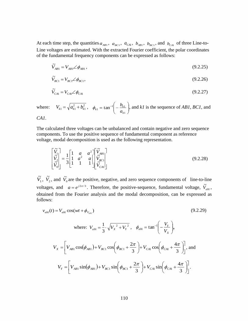
110

At each time step, the quantities1ABa ,

1BCa , 1CAa , 1ABb ,

1BCb , and 1CAb of three Line-to-

Line voltages are estimated. With the extracted Fourier coefficient, the polar coordinates

of the fundamental frequency components can be expressed as follows:

111

~ABABAB VV , (9.2.25)

111

~BCBCBC VV , (9.2.26)

111

~CACACA VV (9.2.27)

where: 2

1

2

11 kkk baV ,

1

11

1 tank

kk

a

b , and k1 is the sequence of AB1, BC1, and

CA1.

The calculated three voltages can be unbalanced and contain negative and zero sequence

components. To use the positive sequence of fundamental component as reference

voltage, modal decomposition is used as the following representation.

1

1

12

2

0

2

1

~

~

~

11111

3

1

~

~

~

CA

BC

AB

V

V

V

aaaa

V

V

V

(9.2.28)

1

~V , 2

~V , and

0

~V are the positive, negative, and zero sequence components of line-to-line

voltages, and 3/2jea . Therefore, the positive-sequence, fundamental voltage, 1

~abV ,

obtained from the Fourier analysis and the modal decomposition, can be expressed as

follows:

)cos()(111 abVabab wtVtv (9.2.29)

where: 22

13

1YXab VVV ,

X

Yab

V

V1

1 tan ,

3

4cos

3

2coscos 111111

CACABCBCABABX VVVV , and

3

4sin

3

2sinsin 111111

CACABCBCABABY VVVV .

111

Based on the same procedure, the positive-sequence fundamental output-voltage van1(t)

and output-current ia1(t) are computed, and output power is also computed using the

positive-sequence fundamental output voltage and current.

Cosine-wave crossing method is a popular scheme, since it minimizes the total harmonic

distortion (THD) of output-voltages [44][49] and it is a simple method to be implemented

for the three-phase six-pulse cycloconverter. Since the three-phase six-pulse

cycloconverter interconnects a low-frequency system (16.66/20Hz) with normal power

grids (50/60Hz), harmonic distortion is an important power quality issue, and harmonic

filter size depends on it. For minimizing the impacts from harmonics, a sophisticated

control algorithm is needed for the three-phase six-pulse cycloconverter, and the cosine-

wave crossing method with full- or partial-circulating currents is proposed in this chapter.

In cosine-wave crossing method, the firing pulses for thyristors are generated at crossing

points of cosine-wave (which is named wanted output-voltage) and estimated-voltage

references that are emulated by the reference voltage, vab1(t). The whole processes are

shown in Figure 9.2.5.

Generate wanted

voltages

Pulse generater of

both converters

Current sensing

and bank selection

Close loop control

logic

Step 1 Step 2 Step 3

Step 4Step 5Step 6

Generate voltage

references

Transmit firing pulse

to thyristors

Figure 9.2.5: Control Algorithm for the Cycloconverter

In Step 1, the positive-sequence fundamental input-voltages are generated based on the

positive-sequence fundamental input-voltage Vab1(t). Note that Vab1(t) is the estimated

value from DSP. The reference voltages are computed as follows:

)cos()(11 abViabab twVtV (9.2.30)

)60cos()(11

o

Viabac abtwVtV (9.2.31)

)120cos()(11

o

Viabbc abtwVtV

(9.2.32)

)180cos()(11

o

Viabba abtwVtV (9.2.33)

)240cos()(11

o

Viabca abtwVtV (9.2.34)

)300cos()(11

o

Viabcb abtwVtV (9.2.35)

112

where wi is angular velocity at high-frequency side.

Since the output-voltages at the low-frequency side are not the same to the wanted

voltages (output-voltages are normally bigger than wanted voltages), a closed-loop

controller is used to regulate the wanted voltages and equate the output-voltages and the

voltage order. Here, we use two closed-loop controllers for magnitude and phase angle of

the wanted voltage. Since the closed-loop controller for the magnitude is almost the same

to that of the phase angle, the closed-loop controller for the phase angle of wanted

voltage is only presented in this report. The process is implemented in Step 2 and the

closed-loop controller for the phase angle is shown in Figure 9.2.6. Note that the phase

angle is used to control the output power.

+-

Pord

Pest

u1

u2

x1 =ErrPI

∆δ+

-

δ(t-h)

δ(t)-

θ

+

2

θ1

Figure 9.2.6: Close Loop Control Algorithm for (a) Magnitude of Voltage and (b)

Output Power

The state-space equations of the control algorithm are represented as follows:

)()()(0 211 tututx (9.2.36)

121 xkxxk Ip (9.2.37)

)()()(0 332 tutxtx (9.2.38)

)()()(0 443 tutxtx (9.2.39)

where: Testord

Thtppuuuuu 24321 )( ,

TTErrxxxxx 14321 , and Pord is power order, Pest is the

estimated power from the DSP, θ1 is the phase angle at output voltage (van) of the

cycloconverter, θ2 is the phase angle at loads, and δ= θ1 – θ2.

Note that the algebraic-companion form of the power controller can be also calculated

upon application of the quadratic integration, and the algebraic companion-form of the

controller can be integrated to the three-phase six-pulse cycloconverter. The process is

the same to the modeling process of the single-phase transformer in subsection A in this

chapter.

In Step 3, the wanted voltages are computed, based on the outputs of the closed-loop

controllers. The wanted voltages can be computed as follows:

113

)cos()( 1 twVtV owantwa (9.2.40)

)120cos()( 1

o

owantwb twVtV (9.2.41)

)240cos()( 1

o

owantwc twVtV (9.2.42)

where wo is angular velocity at low frequency side, and Vwant and θ1 are the magnitude

and phase angle from closed-loop controllers.

In step 4, firing pulses for thyristors can be generated at the point Vw(t)= VT (t) for both

positive converter and negative converter. VT is the average values of two adjacent

estimated input-voltages from the DSP. For an example, assuming that )(tVab and )(tVac

are the adjacent input voltages, then 2

)()()(

tVtVtV acab

T

.

In Step 5, the magnitudes of the output currents can be sensed, and the values can be used

to select either the positive or the negative converters. Assuming that the output-current

Ia(t) is bigger than circulating threshold current TI , the positive converters are activated,

and assuming that the output-current is smaller than TI , the negative converters are

activated. In circulating mode (Ta ItI )( ), both converters are activated. Note that the

circulating threshold current is a determined value from system operators.

In Step 6, the firing pulses are transmitted to the proper converter bank(s). Assuming that

the cycloconverter is working in the full circulating mode, firing pulses are transmitted to

both converters, and the sum of the firing angles for both converters is always 1800.

Otherwise, the firing pulses have to be transmitted to the proper converter bank(s),

according to the output currents and circulating threshold currents..

Note that the control algorithm is repeated at every time-step, until the simulation is over.

9.2.4 Three-Phase PWM Converter

In this subsection, the modeling methodology for the three-phase pulse-width modulation

(PWM) converter is presented. The three-phase PWM converter is used for the

alternative-transmission systems, since phase-controlled converters are impractical for

weak-synchronous systems and induction machines for wind farms. Also, the three-phase

PWM converters have demonstrated several superior properties including: (a) bi-

directional power flow control, (b) low-harmonic distortion of AC-line currents, and (c)

flexible imaginary power control [51]. These converters have to support maximum power

capturing from wind-turbine systems and offer constant output-voltage frequency from

variable speed wind [52]. The three-phase PWM converter consists of six electrical-

valves and a smoothing capacitor as shown in Figure 9.2.7. Furthermore, controllers are

needed to generate switching sequences for on/off-controllable switches of the three-

phase PWM converter. The controllers are based on direct power control algorithm using

114

space vectors, since the controllers have demonstrated rapid dynamic response with

simple structure [53].

Figure 9.2.7: Three-Phase PWM Converter

The electrical-valves in the three-phase PWM converter are the same to those in the

three-phase six-pulse cycloconverter, except that the electrical switches are on/off-

controllable switches. Even though the physical structure of the electrical-valves in the

three-phase PWM converter is different from those of the electrical-valves in the

cycloconverter, the mathematical equations for the valve are equivalent to each other. So,

the electrical-valve model is omitted in this subsection and a smoothing capacitor model

is presented for the three-phase PWM converter. The equivalent circuit of the smoothing

capacitor is shown in Figure 9.2.8.

115

)(2 ti

)(1 ti

0

)(1 tv

)(2 tv

)(tvc

+

-

)(1 ty

1

34

Figure 9.2.8: Three-Phase PWM Converter

The differential equations and algebraic equations describing a smoothing capacitor

model are written in state-space form. There are two sets of equations: external equations

and internal equations. The state-space model of the smoothing capacitor is given as

follows:

)()( 11 tCyti (9.2.43)

)()( 12 titi (9.2.44)

)()(

1 tydt

tdvc (9.2.45)

)()()(0 21 tvtvtvc (9.2.46)

A compact-matrix form can be easily written using the state-space equations above and

the algebraic-companion form is derived by the application of the quadratic integration

method to the compact matrix form. All processes are the same with the case of the

single-phase transformer model in subsection A of this chapter.

9.2.5 Controller Design of the PWM Converter

To control the proposed three-phase PWM converters, direct-power control (DPC)

algorithm is used, since the control algorithm has demonstrated several outstanding

characteristics such as: simple algorithm, superior dynamic response, and steady-state

performance [54]. The control algorithm can be modeled for both (1) constant-frequency

applications and (2) variable-frequency applications. Generally, the three-phase PWM

converter with the constant-frequency control-algorithm, which is named as grid-side

converter (GSC), is directly connected to the grid systems and the GSC supports constant

DC-voltage and reactive-power controllability for grid connected systems. Otherwise, the

PWM converter with variable-frequency control algorithm, which is named as machine-

side converter (MSC), is directly connected to the wind turbines and the MSC support

116

maximum power capturing from wind turbine systems and reactive-power controllability

to them. Note that MSC is directly connected to the rotor of a doubly-fed induction

generator (DFIG) in Type-3 wind-generation unit and the stator of a permanent-magnet

synchronous generator (PMSG) in Type-4 wind-generation unit. Since the control

algorithms of the three-phase PWM converter are very diverse according the control

purpose and controlled devices, all cannot be considered in this section. So, we present

two general control algorithms for both a constant-frequency controller and a variable-

frequency controller as shown in Figure 9.2.9 and Figure 9.2.10. Note we only present

the modeling process of the constant-frequency controller since the space to describe both

controllers is not enough as well as the DPC algorithms for Type-4 wind-generation unit

are easily found in previous researches form [54] to [56].

Active and

Reactive power

estimation

Q

Q +

SVM

dq

PI

PI-

+V

P u u

u u

s a s b s ce ae b i ai b

q d

e c i c

* *

* *

S

-

Three-phase

PWM converter

A

C

B

KD

AD

ref

dc.ref

Vdc

x PI+

-

I *P*

Figure 9.2.9: Constant-Frequency Controller using Direct-Power Algorithm with Space-

Vector Modulation

Active and

Reactive power

estimation

Q

Vector

selection

VectorP

s a s b s ce cse bs

icribr

e as

iar

-

Three-phase

PWM converter

A

C

B

KD

AD

+

csbsasi i i wm

Hysteresis

controller

Hysteresis

controller

P s.ref+

-

+Q s.ref+

DFIM

Pulse

Generationθψr

Pu

Qu

Pe

Qe

Figure 9.2.10: Variable-Frequency Controller using Direct-Power Algorithm with

Hysteresis Controllers

117

Figure 9.2.9 shows a constant-frequency control algorithm and it is based on direct-power

control algorithm with space vector modulation (DPC-SVM). The control algorithm can

be modeled based on the following three steps:

Step 1: Active and real power (P and Q), and synchronous position angle (θs) estimation

Step 2: Voltage-reference estimation in αβ-coordination

Step 3: Switching sequence estimation from SVM algorithm

In Step 1 active- and real-power and synchronous-position angle are estimated with the

same processes of the reference-estimation part in subsection C in this chapter. First the

positive-sequence fundamental three-phase voltages and three-phase currents are

computed and the three references are calculated as follows:

11

cos2

311 aa ivaa IVP (9.2.47)

11

sin2

311 aa ivaa IVQ (9.2.48)

The voltages in αβ-coordination are computed using Clarke direct transformation as

follows:

1

1

1

2

3

2

30

2

1

2

11

3

2

c

b

a

V

V

V

v

v

(9.2.49)

Using the two voltages in αβ-coordination, the synchronous angle-position (θs) is

computed. Therefore, the result is:

v

vanats

(9.2.50)

In step 2, direct power control algorithm is modeled in state-space equations to compute

the reference voltages in αβ-coordination. DPC algorithm is two-state algorithm in which

DC-voltage and reactive-power can be decoupled to each other and controlled separately.

As shown in Figure 9.2.11, three PI-controllers are used to compute the reference

voltages in αβ-coordination.

118

+-

+-

PI

PI Χ +- PI

dqαβ

y2

u1

u2

u3u3

u4

u5

u6

x1 x2 x7

x3 x4 x5 x6

y1

Figure 9.2.11: Block Diagram of DPC Control Algorithm

Here, we represent the control algorithm into state-space equations. Note U and X is input

vector and state vector of the DPC, respectively, and the vectors are denoted as following

equations in mathematic representation.

Tsdcrefdcref

TPQVVQuuuuuuU .654321

Td

x

dcrefdcqref

TUPPPIVVUQQxxxxxxxX ***

.

*

7654321

The state-equations of the DPC are:

)()()(0 411 tututx (9.2.51)

)()()( 11211 txktxtxk Ip (9.2.52)

)()()(0 323 tututx (9.2.53)

)()()( 32432 txktxtxk Ip

(9.2.54)

)()()(0 543 txtxtu (9.2.55)

)()()(0 565 tutxtx

(9.2.56)

)()()( 63763 txktxtxk Ip

(9.2.57)

119

In the compact matrix form of the state-space equations, the DPC is represented as

follows:

UCXBXA (9.2.58)

where:

10000000000000000000

0001000000000

0000010000000

3

2

1

p

p

p

k

k

k

A ,

0000000110000

001)(000

0000000000100

0000000000001

3

3

2

1

I

I

I

k

tu

k

k

B , and

000000010000000000000000000110000000001001

C .

Note kpj and kIj are constant values for PI controllers and j is integers from 1 to 3.

Using the quadratic integration, the ACF of the DPC can be calculated in the same

modeling processes of the singe-phase transformer in subsection A of this chapter. Since

the state variables of x2 and x7 are the reference voltages ( *

qu and *

du ) in dq-coordination,

the voltages in dq-coordination are transformed into those in αβ-coordination. Finally, the

reference voltages for SVM are computed as follows:

2

7

66

66

x

x

uu

uu

u

u

cossin

sincos*

*

(9.2.59)

In step 3, the SVM diagram in Figure 9.2.12 is used to calculate on- and off-switching

times of the electrical-switches. The SVM is one of digital control algorithms for the

three-phase PWM converter connected to constant-frequency systems. According to the

reference voltage on the diagram, switching times and switching sequence are decided.

First, the reference voltage on the SVM diagram can calculated using the reference

voltages ( *

u and *

u ) from the DPC algorithm as follows:

refsvmrefsvm VV .,

, (9.2.60)

120

where 2*2*

. )()( uuV refsvm and

*

*

u

uanta .

The dwelling time (pulse-width) that denotes switching time is calculated based on volt-

second balancing principle as follows. Note Ta, Tb, and Tc are the dwelling times of the

three legs of phase A, phase B, and phase C, respectively.

3sinaSa mTT , (9.2.61)

sinaSb mTT ), and (9.2.62)

baS TTTT 0 (9.2.63)

where: dc

ref

aV

Vm

3 ,

3)1(

n , and n is the section number in the SVM

diagram. Note the modulation index ma is in the range of 10 am .

Vsvm.ref

θα

(POO)

V1

V2

V3

V4

V6

V5

(PPO)(OPO)

(OPP)

(OOP) (POP)

Section 1

Section 2

Section 3

Section 4

Section 5

Section 6

(POO)

V1

V2

V3

V4

V6

V5

(PPO)(OPO)

(OPP)

(OOP) (POP)

Section 1

Section 2

Section 3

Section 4

Section 5

Section 6

Clockwise

Counterclockwise

a

b

a

a

a

a

a

b

b

b

b

b

Figure 9.2.12: (A) SVM Diagram and (B) Mirror Image in SVM Diagram

After the dwelling times are computed, the switching sequence is arranged for the three-

legs based on seven–segment arrangement and even-order harmonics elimination method .

We select the switching sequence in the following requirements [57]:

During the transition from one state to another state, only two switches in the

same leg have to be involved.

During the transition from one section to another section in the SVM diagram,

none or minimum number of switching is required.

121

As well known, waveforms of half-wave symmetry should not contain any even-order

harmonics. To achieve the half-wave symmetry, two regions facing each other in the

SVM diagram can be arranged in a mirror image. Note that the switching sequences

rotate clockwise or counterclockwise as shown in (B) of Figure 9.2.12 and the line-to-line

voltages are achieved in half-wave symmetrical forms.

9.3 Power-Transient Studies of LFAC Transmission Systems

For the power-transient studies, we introduce two wind farm configurations using the

LFAC transmission system. The first wind farm configuration is using a parallel low-

frequency wind farm and a low-frequency radial AC transmission system as shown in

Figure 9.3.1, and the second configuration is using a series DC wind farm and a low-

frequency radial AC transmission system as shown in Figure 9.3.5. Using the two wind

farm configurations, the power transient studies are performed. In this simulation, the

power step change suddenly occurs while the LFAC transmission system is operating in

steady state.

Case 1: Wind Farm configuration: LFAC wind farm and LFAC transmission system

This Case 1 presents simulation results on an example wind farm with a LFAC

transmission system connected to a power grid, as shown in Figure 9.3.1. The wind farm

consists of many wind-turbine systems - the example system includes three of them. The

wind generated power is rectified to DC and then it is converted to 20 Hz AC power. A

transformer boosts the voltage to 46-kV. A LFAC line operated at 46-kV transmits the

power over a distance of 100-km to the nearest power grid substation. At that point a

cycloconverter converts the 20 Hz AC-power into 60 Hz AC-power and another

transformer boost the voltage to 115-kV for the interconnection. The transformer is

connected to the power grid which is a 115-kV, 60 Hz transmission at that point. The

three-phase six-pulse cycloconverter is operating in a full circulating-current mode and

the control algorithm for generating the switching pulses is the cosine-wave crossing

122

method.

Figure 9.3.1: Wind Farm Configuration: LFAC Wind Farm and LFAC Transmission

Each wind turbine/generator system consists of a wind-turbine, full-rectifier and full-

inverter that converts the power into 20 Hz AC power and a transformer that boost the

voltage to 46 kV. The power from all wind turbine/generator systems are collected to a

common point and the total power is transmitted via a LFAC transmission line to the

interconnection point with the power grid. The interconnection is achieved with the

cycloconverter and the step-up transformer. The LFAC system was simulated in a

transient condition. Specifically, while the system is operating with 4 MW through the

LFAC line, suddenly the wind power changes to the point that requires the LFAC line to

transmit 9 MW.

Figure 9.3.2 represents three-phase (a) line-to-line voltages and (d) currents at the 60Hz

AC transmission system connected to the three-phase six-pulse cycloconverter, three

phase (c) voltages and (b) currents at the LFAC transmission system connected to the

three-phase six-pulse cycloconverter, and the (e) real power from wind farm and the (f)

RMS voltage at LFAC, while power demand suddenly changes 4MW into 9MW at 3

second. Figure 9.3.3 shows the results during the transient condition from 2.80 to 3.40

(seconds) - zoom-in view, and Figure 9.3.4 represents the results during steady state from

6.75 to 7.00 (seconds). Note that the output power can be automatically regulated by

controlling the power angle δ. The transient conditions last shorter than 0.15 seconds.

123

101.2

-101.2

0.0

467

-467

0.0

58.2

-58.2

0.0

188.0

188.0

0.0

9.00

0.0

54.8

0.0

0.0 1.17 2.33 3.5 4.67 5.83 7.0

KV

KV

A

A

MW

(a)

(b)

(c)

(d)

(e)

(f)

KV

Figure 9.3.2: Three-Phase (a) Line-to-Line Voltages and (d) Currents at 60Hz AC

Transmission Connected to the Cycloconverter; Three-Phase (c) Voltages and (b)

Currents at LFAC Transmission Connected to the Cycloconverter; and (e) Real Power

from Wind Farm and (f) RMS Voltage at the LFAC from 0.0 to 7.0 Seconds

99.0

-99.0

0.0

404.0

-404.4

0.0

58.1

-58.1

0.0

157.2

-157.20.0

7.68

4.01

47.2

46.7

2.80 2.89 2.98 3.07 3.16 3.25 3.40

KV

KV

A

A

MW

(a)

(b)

(c)

(d)

(e)

(f)

KV

Figure 9.3.3: Three-Phase (a) Line-to-Line Voltage and (d) Currents at 60Hz AC

Transmission Connected to the Cycloconverter; Three-Phase (c) Voltages and

(b) Currents at LFAC Transmission Connected to the Cycloconverter; and (e) Real Power


124

97.7

-97.7

0.0

468.0

-468.4

0.0

57.1

-57.1

0.0

188.5

-188.50.0

9.0

8.99

46.3

46.2

6.75 6.73 6.83 6.87 6.92 6.96 7.00

KV

KV

A

A

MW

(a)

(b)

(c)

(d)

(e)

(f)

KV

Figure 9.3.4: Three-Phase (a) Line-to-Line Voltage and (d) Current at 60Hz AC

Transmission Connected to the Cycloconverter; Three-Phase (c) Voltages and (b)

Currents at LFAC Transmission Connected to the Cycloconverter; and (e) Real Power


Case 2: Wind Farm configuration: DC wind farm and LFAC transmission system

This case study presents simulation results on an example wind farm with a LFAC-

transmission system connected to a power grid, as shown in Figure 9.3.5. The wind farm

consists of many wind turbine systems - the example system includes three of them. The

wind-turbine systems are connected in series after the wind generated power is rectified

to DC, and the DC-power is converted to 20 Hz AC-power using an inverter. A

transformer boosts the voltage to 46-kV. A LFAC line operated at 46-kV transmits the

power over a distance of 80-Km to the nearest power grid substation. At that point a

cycloconverter converts the LFAC power into 60 Hz AC-power for the interconnection

and another transformer boost the voltage to 115 kV. The transformer is connected to the

power grid which is a 115-kV, 60 Hz-transmission at that point.

125

Figure 9.3.5: Single-Line Diagram of a Power Transient Test System

The results illustrate the operation of the wind farm transmission system by using a three-

phase six-pulse cycloconverter. The three-phase six-pulse, cycloconverter is operating in

a partial circulating current mode and the control algorithm for generating switching

pulses is the cosine-wave crossing method.

Figure 9.3.6 represents three-phase (a) line-to-line voltages and (b) currents at the 60Hz

AC transmission system connected to the three-phase six-pulse cycloconverter; three-

phase (c) voltages and (d) currents at the LFAC-transmission system connected to the

three-phase, six-pulse cycloconverter; and the (e) real power from wind farm and the (f)

RMS voltage at LFAC during 10 seconds. In this simulation, the power demand changes

6MW into 10MW at 5 second.

Figure 9.3.7 and Figure 9.3.8 represent three-phase (a) line-to-line voltages and (b)

currents at the 60Hz AC transmission system connected to the three-phase, six-pulse

cycloconverter, and three-phase (c) voltages and (d) currents at the LFAC- transmission

system connected to the three-phase, six-pulse cycloconverter in steady state. In Figure

9.3.7, the power demand is 6-MW and the operation mode is a partial circulating-current

mode of 0.7-pu of the phase currents at the LFAC side. The Figure 9.3.8 shows the

results with following conditions: the power demand is 10MW and the operation mode is

a partial circulating-current mode of 0.4-pu of the phase current at the LFAC side.

126

99.6

-99.6

0.0

131

-1310.0

62.9

-62.9

0.0

205

-205

0.0

10.04

0.0

53.0

0.0

0.0 1.65 3.30 4.95 6.60 8.25 10.0

KV

KV

A

A

MW

(a)

(b)

(c)

(d)

(e)

(f)

KV


60Hz AC Transmission Connected to the Cycloconverter; Three-Phase (c) Voltages and

(b) Currents at LFAC Transmission Connected to the Cycloconverter; and (e) Real Power


99.6

-99.6

0.0

127

-127

0.0

62.9

-62.9

0.0

205

0.0

4.846 4.872 4.897 4.923 4.949 4.975 5.0

KV

A

A

(a)

(b)

(c)

(d)

KV

-205


60Hz AC Transmission Connected to the Cycloconverter; and Three-Phase (c) Voltages

and (b) Currents at LFAC Transmission Connected to the Cycloconverter during Steady

State from 4.846 to 5.0 Seconds

127

97.2

-97.2

0.0

106

-106

0.0

49.1

-49.1

0.0

204

0.0

9.785 9.821 9.857 9.892 9.928 9.964 10.0

KV

A

A

(a)

(b)

(c)

(d)

KV

-204


60Hz AC Transmission Connected to the Cycloconverter; Three-Phase (c) Voltages and

(b) Currents at LFAC Transmission Connected to the Cycloconverter during Steady State

from 9.785 to 8.0 Seconds

Figure 9.3.9 and Figure 9.3.10 represent the results in transient conditions: (a) three-

phase currents at the 60Hz AC- transmission system connected to the three-phase, six-

pulse cycloconverter, three-phase (b) voltages and (c) currents at the LFAC-transmission

system connected to the three-phase, six-pulse cycloconverter. Figure 9.3.9 shows the

initial transient condition from 0.0 to 0.5 seconds. The cycloconverter is operated in a full

circulating-current mode while the maximum currents at the LFAC side are smaller than

80 A, and otherwise, the cycloconverter is operated in a partial circulating-current mode.

In Figure 9.3.10, the power demand suddenly changes 6MW to 10MW at 5.0 second.

Note that the output power can be automatically regulated by controlling the power angle

δ. The transient conditions last longer than 1.0 second.

91.0

-91.0

0.0

62.8

-62.8

0.0

121

0.0

0.0 0.083 0.166 0.2489 0.3319 0.4149 0.500

A

A

(a)

(b)

(c)

KV

-121

Figure 9.3.9: (a) Three-Phase Currents at 60Hz AC Transmission Connected to the

Cycloconverter; and Three-Phase (b) Voltages and (c) Currents at LFAC Transmission

Connected to the Cycloconverter during Steady State from 0.0 to 0.500 Seconds.

128

94.8

-94.8

0.0

55.4

-55.4

0.0

170

0.0

4.867 4.959 5.052 5.145 5.237 5.330 5.423

A

A

(a)

(b)

(c)

KV

-170

Figure 9.3.10: (a) Three-Phase Currents at 60Hz AC Transmission Connected to the

Cycloconverter; and Three-Phase (b) Voltages and (c) Currents at LFAC Transmission

Connected to the Cycloconverter during Steady State from 4.867 to 5.423 Seconds

9.4 Harmonics Study of LFAC Transmission Systems

The wind farm configuration in Figure 9.3.1 is used for harmonics study. The operating

voltage at high-frequency side is 70-kV (RMS) and the operating voltage at low-

frequency side is changed to regulate the modulation index of the three-phase six-pulse

converter since the harmonics depend on the modulation index. The electrical power of

10 MW is transmitted from wind farm to grid systems. Note that the modulation index (r)

is computed as following equation:

o

inputLL

outputa

V

Vr

30cos

(9.3.1)

where Va-output is the phase voltage at the low-frequency side and VLL-input is the line-to-line

voltage at the high-frequency side.

Figure 9.4.1 shows the simulation results in modulation index 1.0 in full circulating-

current mode: (A) the line-to-line voltage between phase A and phase B and (B) the

current at phase A; and (C) the phase-voltage and (D) the phase-current at phase A. The

harmonics are computed using Fourier-series analysis and the harmonic spectrums are

presented in logarithmic scale for the currents and voltages at both sides of the

cycloconverter as shown in Figure 9.4.2. Note that the harmonic order is computed as

follows:

frequencylfundamenta

frequencyhighorderHarmonic (9.3.2)

where the fundamental frequency is 60 Hz at the HFAC side and 20 Hz at the LFAC side.

129

Figure 9.4.1: (A) Line-to-Line Voltage between Phase A and Phase B; (B) Current at

Phase A; (C) Phase Voltage and (D) Phase Current at Phase A

(A) Harmonic spectrums of line-to-line voltage at the HF side (B) Harmonic spectrums of phase-current at the HF side

(C) Harmonic spectrums of Phase-voltage at the LF side (D) Harmonic spectrums of phase-current at the LF side

Figure 9.4.2: Harmonic Spectrums: (A) Line-to-Line Voltage between Phase A and

Phase B, (B) Current at Phase A, (C) Phase Voltage at Phase A, and (D) Phase Current at

Phase A

130

Table 9.4.1 presents numerical values of the harmonic spectrums of the phase-voltage at

the low-frequency side of the cycloconverter and Figure 9.4.3 shows the graphs of the

numerical values. In this study, the modulation index is changed from 0.38 to 1.0 and the

harmonics is recorded according to the modulation index. As shown in Table 9.4.1 and

Figure 9.4.3, the modulation index is an important parameter since the harmonic contents

depend on it. While the modulation index approaches zero, the THDs are substantially

increasing; otherwise, while the modulation index approaches one, the THDs are

decreasing. Therefore, the modulation index between 0.75 and 1.00 assures the small

filter size for the cycloconverter.


Modulation

Index ma

Harmonic Order

3 5 7 9 11 13 15 17 19 21 THDs

1.00 0.41 0.62 1.2 1.8 1.7 8.9 8.3 3.8 2.9 8.1 20.1

0.88 1.4 1.6 1.8 0.87 0.8 6.3 8.7 3.3 4 8.3 22.52

0.75 2 1.8 2.1 0.51 1.1 4.6 8.7 8.1 8.4 8.3 26.43

0.63 3.9 3.3 1.8 0.22 0.69 3 8.6 20 22 8.1 33.78

0.50 8 3 1 0.77 2.5 8.9 8.9 31 30 6.5 42.14

0.38 17 4.8 3.7 1.4 1.2 0.4 0.04 39 37 2.4 48.87

Unit: percentage (%)

40

35

30

25

20

15

10

5

03 5 7 9 11 13

15 17 19 211.00

0.880.750.630.500.38

1.000.880.750.630.500.38

Percentage (%)

Harmonic Order

Modulation

index (Ma)

Ma

Figure 9.4.3: Harmonic Spectrums of the Phase Voltage at the LFAC Side

131

Next test presents the harmonics comparison between full- and partial- circulating current

modes. For the purpose, the same modulation index is used for both cases. The

modulation index is 0.38 and the magnitude of threshold current (IT) is the half of the

maximum value of the phase-current at the LFAC side of the cycloconverter. Table 9.4.2

presents the numerical values of the harmonics contents and Figure 9.4.4 graphically

represents the harmonic spectrums for both modes. As shown in Table 9.4.2 and Figure

9.4.4, the full-circulating current mode presents a smaller total harmonic distortion of the

phase-voltage at the LFAC side than that from the partial-circulating current mode.


Side in Both Full- and Fifty Percent-Circulating Current Modes

Circulating

Mode

Harmonic Order

3 5 7 9 11 13 15 17 19 21 THDs

Full 17 4.8 3.7 1.4 1.2 0.4 0.04 39 37 2.4 48.87

50% 39 17 12 11 4.1 7.9 28 39 29 19 59.67

3 5 7 9 11 13 15 17 19 21

Harmonic Order

THD

40

30

20

10

0

60

50

Pe

rce

nta

ge

(%

) 70

Full circulating-current

50% circulating-current

Harmonic spectrum

Figure 9.4.4: Harmonic Spectrums of the Phase Voltage at the LFAC Side: (Blue) Full

Circulating-Current Mode and (Red) 50% Circulating-Current Mode

132

10 Reliability Analysis of Wind Farm Configurations

This section describes the reliability analysis of the 8 configurations listed in Chapter 4 of

the report. Alternative transmission configurations have been formed by the combination

of AC transmission at nominal power frequency, HVDC transmission, and low frequency

AC transmission. Chapter 4 describes the 8 alternative configurations. These

configurations will be compared from the reliability point of view in this chapter.

The general formulation of the reliability approach is provided in subsection 10.1,

followed by the individual analysis of each of the 8 alternate configurations. For each

configuration, the reliability analysis model is developed first, considering both the

structural reliability model (full capacity model) and wind variability model. In addition,

for each alternative configuration, a 30 wind turbine example is also provided. The

reliability parameters used in each of the examples were assumed since actual reliability

data are not available. The assumed parameters are shown in Appendix F.

10.1 Approach Description

The reliability analysis of any wind farm configuration is performed by assuming that

each component of the configuration has a Monte Carlo model. In other words, each

component is characterized with two basic parameters: failure rate and repair rate.

Assumed values for these parameters are shown in Appendix F. Using these models for

each component, the overall reliability of the wind farm is computed. In order to separate

and quantify the effect of equipment failures from the variability of the wind energy

resource, the overall problem of reliability analysis is separated into two sub-problems:

(a) structural reliability model (full capacity model), and (b) wind variability model. The

definition and relationship between these two models is provided below.

Structural Reliability Model: This model assumes that the wind energy is 100%

reliable. This means that if the wind farm equipments are available, the output of the

wind farm will be equal to the full capacity of the wind farm. For this reason, we shall

also refer to this model as full capacity model.

Wind Variability Model: This model includes the wind variability as well as the

structural reliability model of the wind farm.

The cost analysis of the configurations is provided in Section 5 of the report. The

calculation results of the annual cost of each of the configurations are provided in the

case study part of each subsection, as a reference for the evaluation of reliability. Most of

the time the cost is increasing with reliability, i.e., the configuration with a higher

reliability indices normally accounts for a higher cost, such as connecting in parallel is

more reliable than connecting in series, but requires more acquisition cost. Therefore, the

selection of wind farm is not entirely based on the maximum of reliability or the

minimum of cost, but the optimal combination of both.

133

10.1.1 Structural Reliability Model - Full Capacity Model

In this case, wind speed variation is not considered. This is achieved by assuming that all

wind turbines will generate their full capacity, e.g., a WTS V80-2MW will always

generate 2MW, if available. Generally speaking, the generation capacity of the wind

turbines is denoted as G in the following analysis, and some assumptions are made:

a) All wind turbines are identical, i.e., they have the same generation capacity;

b) All components in the configurations are 2-states components, i.e., they can only

be either “up” or “down” states.

c) Storage components are not considered in the reliability analysis.

d) No transmission constraints are considered.

For each configuration, the specific formulation of reliability analysis calculation is

shown in the following sections. Based on the assumptions above, the reliability analysis

in full capacity case of each configuration will follow the procedure as:

a) Component identification and classification of the configuration;

b) Reliability modeling of each component

c) Reliability modeling of connections, e.g., parallel or series lines

d) Generation capacity probabilistic distribution at PCC

e) Reliability indices calculation

Formulations of reliability calculation will be provided after the analysis, and a 30 wind

turbine case study will be provided in each section as an example.

10.1.2 Wind Variability Model

In this case, wind speed is considered so that the wind turbines are generating at whatever

wind power is available. The reliability index will consider the wind speed distribution.

Wind speed is an important factor that influences the reliability indices especially the

adequacy assessment result of the wind farm. The output of a wind turbine is essentially

influenced by the wind speed. This subsection provides a general description of the

analysis procedure for calculating reliability indices when considering wind speed.

Reference [27] has provided a good analysis of the relationship of wind speed and wind

turbine output power. A typical probability distribution of wind speeds is shown in Figure

10.1.1 created from historical hourly wind data, and a typical WTS power output curve as

a function of wind speed is shown in Figure 10.1.2 for a WTS V80-2MW. Since wind

speed is continuously changing, a probabilistic way is used to assess it and to calculate

the expected value.

134

Figure 10.1.1: Wind Speed Probabilistic Distribution [27]

Figure 10.1.2: A Typical Wind Turbine Output Considering Wind Speed Variation [27]

Figure 10.1.2 provides the output of wind turbine as a function of the wind speed. When

the turbine/generator is in its “up” state, the specific output of the turbine/generator, G(v),

is provided from the mapping shown in Figure 10.1.2, i.e., from the wind speed. For each

speed v, its probability P(v) is as shown in Figure 10.1.1.

135

The expected value of the output of a single turbine is:

∫ [ ]

(10.1.1)

In case of discrete wind speed data, the integral becomes the summation:

∑ [ ] (10.1.2)

The relationship shown in Figure 10.1.2 can be simplified by approximating the given

function with a piecewise linear function, i.e., after cut-in point and before cut-out point

of wind speed, the output power of a wind turbine is almost a linear function of the speed,

which results in the expression of output function:

152000

155)5(200

50

)(

v

vv

v

vG (10.1.3)

which is then used in the evaluation of the integral (10.1.1) or summation (10.1.2) above.

Using the single turbine generating system analysis, the effect of wind speed variation is

modeled as a modification to the constant generation capacity G in the full capacity case,

i.e., G is substitute by E(G) provided by (10.1.1) or (10.1.2) in wind variable model.

In the following sections, the wind speed variation case is analyzed for every

configuration, provided after the full capacity case.

10.2 Reliability Analysis of Wind Farm Configuration 1

In this subsection, Configuration 1 is analyzed from the reliability point of view. This

analysis is provided as an example of the analysis of all the 8 configurations, and is

therefore explained in detail. In the subsequent subsections, the reliability analysis of

Configuration 2 to 8 is performed in the similar way as shown in this subsection for

Configuration 1.

Configuration 1 is shown in Figure 10.2.1. In this configuration, the wind turbine

systems (WTS) generate AC at variable frequency dictated by the wind speed. This is a

simple configuration, without low frequency transmission taken into account.

136

Figure 10.2.1: Wind Farm Configuration 1

In this configuration example 1, there are m parallel circuits of wind generators, each

consisting of series wind turbines respectively. The wind generator output

is AC and all the wind generators in a line are connected in series.

This section describes the reliability analysis of wind farm configuration 1 assuming the

wind turbines are working in full capacity condition and in wind speed variation

condition. The full capacity case refers to the situation that wind is blowing all the time

so that the wind turbines are generating at their full capacity. The wind speed variation

case refers to the situation that the wind turbines generate capacity based on the wind

speed variation.

The reliability analysis in full capacity case is provided first. The objective of reliability

analysis is to provide the probability distribution function of power supply at the point of

common coupling (PCC) assuming that the availability of wind energy is 100%. The end

result will be in the form of a cumulative probability function of the available power at

PCC. This result can be served as the planning and operation index of the power system

operator. The wind speed variation case is provided after the full capacity case.

A list of components in Configuration 1 and their quantities is shown in Table 10.2.1:

137

Table 10.2.1: Components and their Quantities in Configuration 1

Icon Component Total Number of Component

11

Wind Turbine

22

Small Switch

33

Small Transformer

44

In Farm AC Transmission Line

55

Large Switch m

66

AC Bus 1

77

60Hz AC Transmission Line 1

88

Large Substation Transformer 1

In order to simplify the presentation, the following assumptions are made: (a) all the

elements of the same component type are identical, i.e., have the same attributes and

parameters. For example, there are wind turbines in the

configuration, and the assumption is that they have identical failure rates and repair rates;

(b) every component is assumed to be a two-state element, which means it only has “up”

and “down” states. “Up” state represents the successfully working state while the “down”

state represents the failure state of the component; and (c) no transmission constraints are

taken into account. It should be understood that these assumptions are not necessary in

the computer model and analysis.

The reliability parameters of all the components, which include the failure rate and the

repair rate, are listed in Appendix F. The full capacity of each wind turbine is denoted as

G.

In each parallel circuit, a number of components are connected in series. The components

are “dependent” on each other’s success state from the reliability point of view, i.e., if

anyone in the line fails, that line will fail.

Each of the parallel circuits performs “independently” from the others. If one circuit fails,

the other circuits will still be able to operate. At the AC collection bus and subsequent

transmission part, the components are connected in series. These components are

“essential” to the transmission system of the wind farm. If any of the components fails,

the wind farm will not be able to transmit any energy to the power grid. The calculation

of generation capacity levels and their corresponding probabilities are provided as below.

138

10.2.1 Formulation of Reliability Analysis of Configuration 1 in Full Capacity Case

Single Component Probabilistic Model: For component i, the duration of success is

and the duration of failure is

. The probabilities of this component’s being success

and failure are:

(10.2.1)

(10.2.2)

Probabilistic Model of Circuit i: The ith circuit (of the m parallel circuits) is considered.

The ith circuit will be successful in transmitting energy only when all the components in

the line are in their “up” state due to that all generators are serially connected through

each parallel line. Therefore, the states of the ith circuit and the power transmitted in each

state are shown in Table 10.2.2:

Table 10.2.2: States of the ith Circuit and Power Transmitted in Configuration 1

State Power Transmitted Component Status Probability

Up All components “up”

Down 0 At least one “down”

Line up and line down probabilities can be easily obtained by multiplying the up state

probabilities of the components which are connected in series. The success and failure

probabilities of each component can be computed from following formula, in the format

of (10.2.1) and (10.2.2).

Wind Turbine:

;

Small Switch:

;

Small Transformer:

;

In Farm AC Transmission Line:

;

Large Switch:

;

139

Therefore the probability of up state and down state of the ith line can be computed from

formulas shown below.

[ ] (10.2.3)

(10.2.4)

which can be easily obtained by putting the same factors together assuming that in each

category components have the same failure rate of and the same repair rate of .

The complete expressions of the probability of the states of the ith line are:

[ ]

[

]

(10.2.5)

[

]

(10.2.6)

Probabilistic Model of m Parallel Circuits: Since the m circuits are in parallel, the total

generating states depend on the success or failure status of each line. For example, if it is

the case that , the generation capacity states of the m lines are

shown in Table 10.2.3.

Table 10.2.3: States of the m Parallel Circuits (Lines)

State Generation Capacity Probability

1 0

2

3

… … …

m

m+1

The probability of the states is calculated using combinatorial analysis. The (j+1) state,

which has the generation capacity of j n G, has the probability:

(10.2.7)

where

is the combinatorial number; and are

the values calculated in (10.2.5) and (10.2.6).

140

Probabilistic Model of the Entire Configuration: Given the probabilistic model of the

generating section above, i.e., the m parallel circuits (lines), the states of the whole

configuration are determined by the generating section in series with the transmission

section. As an example, the states and corresponding probability when

are shown in Table 10.2.4.

Table 10.2.4: States of Entire Configuration and Probabilities


1 0

2 1 n G

3 2 n G

… … …

m (m-1) n G

m+1 m n G

The success and failure probabilities of components in transmission section can be

computed from the following formula, in the format of (10.2.1) and (10.2.2).

AC Bus:

;

60 Hz AC Transmission Line:

;

Large Substation Transformer:

;

When , the probability of the (j+1)th state, which is the probability of transmitting

power of j∙n∙G, is:

{[

]

}

{ [

]

}

(10.2.8)

This probability is denoted as P(j+1), for all .

141

When , the probability P(0+1)=P(1) can be calculated as:

∑ (10.2.9)

where P(w+1) is determined by (10.2.8)

Therefore in this simple case, the energy levels of the configuration shown in Figure

10.2.1 at the coupling point with the power grid have a list of states and corresponding

probability shown in Table 10.2.5.

Table 10.2.5: States and Corresponding Probabilities


1 0 P(1)

2 1 n G P(2)

3 2 n G P(3)

… … …

m (m-1) n G P(m)

m+1 m n G P(m+1)

where the probabilities are determined by (10.2.8) and (10.2.9).

Expected Generated Wind Energy (EGWE): In this part, the reliability index of

EGWE is calculated given the probability analysis as above. EGWE is the essential index

to be considered for this configuration. Some of other indices that are important are

shown in next part.

Generally, if we know the output states and the probability of each state such as in Table

10.2.5, EGWE is the expectation of the probabilistic output (in one hour):

∑ (10.2.10)

where Gi is the generation capacity of the ith state.

Note here that EGWE is in term of energy (MWh), and (10.2.10) gives the result in term

of power. Since operating time is easy to be measured, the required EGWE can be

determined by multiplying (10.2.10) by the operating time (in hours).

For the general case, the assumption of should be removed;

each of the m parallel circuits has two states: (a) either transmitting full capacity or (b) 0.

For line i, the expected transmitted capacity to the collector AC bus is:

= (10.2.11)

The total expected available energy at point of common coupling is the index of EGWE:

142

[∑

]

[∑

]

∑ { [

]

}

(10.2.12)

10.2.2 Reliability Analysis of Configuration 1 Considering Wind Speed

Using the single turbine generating system analysis, the effect of wind speed variation is

modeled as a modification to the constant generation capacity G in the full capacity case.

The total output expectation at a certain point of time is still in the form of

∑{

[

]

}

as in equation (10.2.12), but G is changed into G(v) at that time point as the function of

the wind speed. For a given period of time with the wind speed probability distribution as

Figure 10.2.1, the expectation of output energy will be:

∑ [ ] ∑ { [

]

}

(10.2.13)

It is shown from (10.2.13) that the influence of wind speed on the calculation of the

expectation is simply a modification by substituting the constant turbine output by the

expectation of that turbine output.

The expected value of the total output is the index of EGWE in a single second. This

index is an averaging assessment of the output power of the wind farm, which can be

used as reference for power system planning and operation control. The next section will

include the calculation of most of the other indices.

10.2.3 Reliability Indices Calculation

This section describes the calculation method of most reliability indices associated with

the wind farm, taking configuration 1 as the analysis objective. The definition and the

formula of these indices, including EGWE, are shown in Table 10.2.6.

143

Table 10.2.6: Definition and Expression of Reliability indices

Reliability Index Expression

Installed Wind Power (IWP) IWP=∑ m f u f m

Installed Wind Energy

(IWE) IWE = Installed Capacity Number of Operating Hours

Expected Available Wind

Energy (EAWE) EAWE=∑ y u y u

Note: components’ possible failure is not included

Expected Generated Wind

Energy (EGWE) EGWE= ∑ y ff y y u

Note: components’s failure is considered

Capacity Factor (CF) CF=EGWE / IWE

Generation Ratio (GR) GR= power delivered to PCC / IWP

wind speed and failure of components are considered.

Expected Generated Wind Energy (EGWE) and Expected Available Wind Energy

(EAWE):

In this part, the reliability indices of EGWE and EAWE will be calculated.

EGWE is discussed much in detail in the sections above, including the calculation

methods both in full capacity case and wind speed variation case. Formula (10.2.12) and

(10.2.13) have provided the expression of EGWE.

EAWE stands for Expected Available Wind Energy, which is the index to evaluate the

available wind power, i.e., the available wind energy in a second. Commonly, wind speed

variation is considered.

∑ (10.2.14)

where E(G) is the expected turbine output determined by (10.1.1) or (10.1.2). In this case,

the wind speed variation is considered, but the transmission failure due to the failure of

components is not considered. This is how EAWE is different from EGWE.

Installed Wind Power (IWP), Installed Wind Energy(IWE), Capacity Factor (CF), and

Generation Ratio (GR):

In this part, the reliability indices of IWP, IWE, CF and GR are calculated based on

the result of EGWE and the probability analysis provided above.

Given the definitions and expressions in Table 10.2.6, the indices are calculated for

configuration 1 as:

∑ (10.2.15)

144

where is the total number of wind turbines in the farm, and G is

the nominal capacity of a single wind turbine in full capacity case.

∑ y f u (10.2.16)

where t is the number of operating time in hours.

CF=EGWE / IWE (10.2.17)

GR= (EGWE/t)/ IWP (10.2.18)

where EGWE is the index calculated by (10.2.8) with both wind speed variation and

transmission failure considered.

10.2.4 Case Study: A 30 WT Case of Configuration 1

An example reliability analysis is shown in this section, using the configuration in Figure

10.2.1. The parameters of the configuration are: (a) Number of parallel lines: m=3; (b)

Number of wind turbines in each Line: ; (c) Generating Capacity of

each Turbine: G = 2MW. Wind speed distribution and the wind turbine output function

are shown in Figures 10.1.1 and 10.1.2. The configuration in this case study is shown in

Figure 10.2.2.

Figure 10.2.2: A 30 WT Case Study Configuration for Configuration 1

Reliability parameters used for this example calculation is shown in Appendix F.

Full Capacity Case: In full capacity case, the calculation result of the output

probabilistic distribution is shown in Table 10.2.7. The essential reliability index EGWE

= 49.42 MWh in one hour.

145

Table 10.2.7: Case Study Output States and Probabilities

State Generation Capacity(MW) Probability

1 0 0.06291222

2 8 0.00861636

3 16 0.08026351

4 24 0.33229952

5 32 0.51590836

The other reliability indices are calculated as:

∑ MW in one

hour.

Note here the indices of EGWE and EAWE is calculated in one hour basis. In order to get

the indices within a certain period, the operating time should be multiplied. For example,

if the indices for a year is needed, the calculation of EGWE and EAWE should be

and respectively.

∑

=60 MWh in one hour

where t is the number of operating time in hours.

CF=EGWE / IWE = 0.824

GR= EGWE / IWP=49.42/60= 82.4%

Wind Speed Variation Case: When wind speed is considered, the single wind turbine

output function is shown in (10.1.1). From the wind speed probability distribution, the

expected output of a single wind turbine becomes ∑ [ ]

MWh. From (10.2.13), ∑ [ ] ∑ [ (∏

)

] ∏

=22.98MWh, which is the reliability index EGWE in one hour.

The result shows the expected generation capacity that can be transmitted to the point of

common coupling. This expected value can be used for system planning and operation.

∑ MWh

in one hour.

146

∑

= 60MWh in one hour, where t is the

number of operating hours.

CF=EGWE / IWE = 22.98/60 = 0.383

GR= EGWE / IWP=22.98/60= 38.3%

The results of the reliability analysis for alternate configuration 1 are summarized in

Table 10.2.8.

Table 10.2.8: Summary of Reliability Indices for Alternate Configuration 1

Reliability Index Computed Value

Installed Wind Power (IWP) 60 MW

Installed Wind Energy (IWE) 60 MWh in one hour

Expected Available Wind Energy (EAWE) MWh in one hour

Expected Generated Wind Energy (EGWE) 22.98MWh in one hour

Capacity Factor (CF) 0.383

Generation Ratio (GR) 38.3 %


This section provides the reliability analysis and case study result for configuration 2.

Figure 10.3.1 shows configuration 2. Configuration 2 has AC Wind Farm and DC

Transmission.

147


The formulation of the reliability analysis for this configuration is as below. The

probabilistic methods used for this formulation are exactly the ones shown in the analysis

of configuration 1.

10.3.1 Probabilistic Model of Circuit i

This configuration has m parallel lines, each line consisting of n wind turbines. The

probability of the states of each line is provided as below.

[

]

[

]

[

]

10.3.2 Probabilistic Model of m Parallel Circuits

The m lines are in parallel, and the probability of having j lines up is shown as below.

148

where

is the combinatorial number.

10.3.3 Probabilistic Model of the Entire Configuration

The output states at the point of common coupling (PCC) are similar to the ones in

configuration 1. At PCC, there are m+1 states, the delivered capacity of which is similar

to that in the analysis of Configuration 1. The 1st state represents the situation when there

is no capacity successfully delivered.


power of , is:

{[

]

}

{

[

]

}



∑

10.3.4 Expected Generated Wind Energy (EGWE)


[∑

]

149

[∑

]

∑{

[

]

}

10.3.5 Case Study

A 30 turbine case is also studied for configuration 2. The parameters of the connection in

the configuration are:

1) m=3, which means there are 3 parallel lines;

2) n=10, which means there are 10 turbines in each line.

The formulation of the calculation is as below.

[∑

]

[∑

]

∑{

[

]

}

=60 MW

=60 MWh in an hour.

In full capacity case,

EGWE=48.21 MWh in an hour

150

EAWE = 60 MWh in an hour

In wind speed variation case,


EAWE = 27.9 MWh in an hour


Table 10.3.1.








Generation Ratio (GR) 37.4%


This section describes the reliability analysis and case study result for configuration 3.

Figure 10.4.1 shows configuration 3. Configuration 3 has DC Series Wind Farm and AC

Transmission.

151



probabilistic methods used for this formulation is exactly the ones shown in the analysis

of configuration 1.


This configuration has m parallel lines, each line consisting of n wind turbines. The

probability of the states of each line is provided as below.

[

]

[

]

[

]


The m lines are in parallel, and the probability of having j lines up is shown as below.

152

where

is the combinatorial number








{[

]

}

{

[

]

}



∑



[∑

]

[∑

]

153

∑{

[

]

}

10.4.5 Case Study






[∑

]

[∑

]

∑{

[

]

}

=60 MW

=60 MWh in an hour.




154





Table 10.4.1.











Figure 10.5.1 shows configuration 4. Configuration 4 has DC Parallel Wind Farm and

AC Transmission.

155




of configuration 1.


In this configuration, there are assumed to be m DC buses, each bus consist of n parallel

connected wind turbines.

10.5.2 Probabilistic Model of m Buses

156

where



The configuration contains m buses and each bus contains n wind turbines. This case is

more complicated than the previous configurations.

Some assumptions need to be made.

1) Transmission Constraints are not considered.

2) All DC buses are identical.

3) All inter-transmission lines, which are the lines connecting the transmission lines,

are identical.

4) All transmission lines, which are the lines connecting the DC bus with the point

of common coupling, are identical.

With these assumptions, the probability of a wind turbine generation’s successful

transmitting to point of common coupling (PCC), is the multiplication of the probability

of its successful transmitting to the DC bus with its successful transmitting from DC bus

to PCC. In addition, the probability of the successful transmission for each turbine is

identical.

The successful transmission from a DC bus to PCC contains many cases. However, the

unsuccessful transmission from a DC bus to PCC, is limited to 2 cases: a) all transmission

lines fail, and b) the transmission line connected to this DC bus fails, and at the same

time, the inter-transmission lines connected to this DC bus fail.

Therefore, the power reaches the transmission line can be delivered to the power system

unless all of the transmission is not successful.

The probability of at least one transmission line works is

The probability of the DC bus, converter and 20Hz transformer will work is

For the convenience of computation, the probability of the internal transmission line that

can deliver the power to transmission line is:

So the probability of the right part of this configuration will work is

157

For

[

]

For

For m

[


∑

For the general case, each of the mn parallel circuits has two states: (a) either transmitting

full capacity or (b) 0. For line i, the expected transmitted capacity to the collector AC bus

is:

=


[ (

) ]

[

]

10.5.5 Case Study



1) m=3, which means there are 3 buses;

158

2) n=10, which means there are 10 turbines on each bus.


[

( ) ]

[ (

)

]

=60 MW

=60 MWh in an hour.







159


Table 10.5.1.











Figure 10.6.1 gives out configuration 5. Configuration 5 has DC Series Wind Farm and

LFAC Transmission (single branch).




of configuration 1.


Since the generators are in series, the system won’t be up unless all the components are

up. Therefore, the number of wind turbine power that is delivered successfully, j ,is either

0 or m.

When , the probability of the state is:

[

]

160

[

]


∑



[

] ( ) ( )

(

) ( ) ( ) ( ) ( )

[

]

10.6.3 Case Study






[

]

(

)

[

]

= 13.2399G

=60 MW

161

=60 MWh in an hour.








Table 13.6.1.









162



Figure 10.7.1 gives out configuration 6. Configuration 6 has DC Parallel Wind Farm, and

LFAC Transmission (single branch).




of configuration 1.


The probabilities of the states of the ith circuit are developed.

163


where









{

}

{

}



∑



[∑

]

[∑

]

164

∑ {

10.7.5 Case Study






[∑

]

[∑

]

∑{

=27.8086G

=60 MW

=60 MWh in an hour.




165





Table 10.7.1.











Figure 10.8.1 gives out configuration 7. Configuration 7 has DC Series Wind Farm,

LFAC Transmission (multiple branches).

166




of configuration 1.


[

]

[

]

[

]

167


where



This configuration has network transmission system. The probability method used to

analyze the network is exactly the one to analyze a single branch. Since in the network

transmission case, the variables related to the number of wind turbines are more than that

of a single branch, by including the number of buses, the number of parallel circuits, and

the number of turbines on a single circuit. This variability makes the formulation of the

probability of this entire configuration complicated, by involving multiple combinatorial

numbers. In this subsection, the single branch case is analyzed to provide the method that

is to be used for more complex cases.

When the transmission system contains only one branch, the output states at the point of

common coupling (PCC) are similar to the ones in configuration 1. At PCC, there are

m+1 states, the delivered capacity of which is similar to that in the analysis of

Configuration 1. The 1st state represents the situation when there is no capacity

successfully delivered.



{[

]

}

{ [

]

}



168

∑



[∑

]

[∑

]

∑ { [

]

}

10.8.5 Case Study






[∑

]

[∑

]

169

∑{

[

]

}

=60 MW

=60 MWh in an hour.








Table 10.8.1.

170











Figure 10.9.1 gives out configuration 8. Configuration 8 has DC Parallel Wind Farm,

LFAC Transmission (multiple branches).




of configuration 1.

171


The probabilities of the states of the ith circuit are provided.


where



The configuration contains m buses and each bus contains n wind turbines. This case is

more complicated so that some assumptions need to be made. Firstly, a single AC

transmission line is supposed to be able to transmit the whole capacity. Therefore, the

power reaches the transmission line can be derived to the power system unless all of the

transmission lines are broken down.

The probability of at least one transmission line works is

The probability of the DC bus, converter and 20Hz transformer will work is

For the convenience of computation, the probability of the internal transmission line that

can deliver the power to transmission line is

So the probability of the right part of this configuration will work is

172

For

[

]

For

For m

[


∑

For the general case, each of the mn parallel circuits has two states: (a) either transmitting

full capacity or (b) 0. For line i, the expected transmitted capacity to the collector AC bus

is:

[ ]

[

]

10.9.5 Case Study






173

[ ]

[ (

)

]

= 28.2625G

=60 MW

=60 MWh in an hour.








Table 10.9.1.

174









10.10 Summary and Conclusions

Section 10 provides the general reliability analysis methods for the configurations listed

in Section 4. For each configuration, a specific modeling and analyzing process has been

shown in a subsection, as provided above from Subsection 10.2 to Subsection 10.9. A 30

wind turbine case study is performed after the analysis of every configuration. The

calculation results have been provided and compared. Table 10.8.1 provides the summary

of the essential reliability indices results from the case studies of the 8 configurations.

Table 10.10.1: Summary of Reliability Indices for the 8 Alternate Configurations

Configuration EGWE IWP CF

1 22.98 60 0.383

2 22.42 60 0.374

3 20.82 60 0.347

4 26.22 60 0.437

5 12.31 60 0.205

6 25.86 60 0.431

7 20.54 60 0.342

8 26.27 60 0.438

It can be understood that the decision of alternate wind farm or transmission technology

selection is not completely based on the reliability analysis, but these results are of

significant value as the assessment criteria.

175

11 Conclusions

Alternative transmission systems from remote wind farms to the main power grid using

low-frequency AC (LFAC) technology are evaluated in this report and compared when

appropriate to conventional AC transmission systems and DC transmission systems. The

performance of LFAC is assessed from several points of view, i.e. total cost, reliability,

power transfer capability, transient stability and electromagnetic transient performance. A

methodology has been also developed for selection of optimal kV level, equipment rating

and in general design of specific wind farms and transmission.

The methodologies have been demonstrated for the three different selections of

transmission systems for connecting remote wind farms to the main power grid.

Specifically, eight alternative configurations have been defined that incorporate the three

transmission options (conventional AC, DC transmission and low frequency AC

transmission). Each one of these configurations were analyzed with the listed criteria and

the example results have been provided in the report. While the results are applicable to

the example systems selected, the methodology is applicable to any specific site and can

be utilized in the design procedure for these systems.

The results indicate that low frequency AC transmission has economic and performance

advantages over conventional AC and DC transmission when the transmission distance is

above 50 miles. Low frequency AC systems have greater power transfer performance,

lower cost and high reliability. The related issue of existing technology for the easy

implementation of low frequency AC transmission systems and wind generation at

20Hz/16.66Hz is quite achievable since these technologies already exist.

Wind energy is the most rapidly developing generating systems from all renewable

resources and the forecast is that they may be forming a large percentage of the

generation system. For this reason their performance is of paramount importance to the

reliability of the power system of the near and far future. The models developed in this

research project can be utilized to study other very important operational characteristics

and capabilities of this system.

One main concern is that as the percentage of wind generating systems become very large

(even 100% in some systems) what will be the operational challenges of these new

systems from the stability, control, operation and protection point of view. For example

since these systems can almost instantaneously (within a cycle) control voltage and

frequency the traditional control schemes may not work for these systems since now

frequency does not provide the same information (transient response of the system,

frequency response, etc.). New paradigms must be developed for the control of systems

with very large penetration of wind generation. In addition these systems limit fault

currents. This property renders the present protection schemes, that depend on high

separation between fault currents and load currents, ineffective. New protection

paradigms and algorithms must be developed for these systems. Another important area

is the behavior of these systems during faults. This has been recognized and new

requirements have been formulated regarding the response of these systems during faults

under the names, zero voltage ride through capability or disturbance ride through

176

capability. This capability should be integrated with the other issues that we have

discussed earlier.

References

1. X. Wang, H. Dai, and R. J. Thomas, “Reliability modeling of large wind farms and

electric utility interface systems” IEEE Transactions on Power Apparatus and

Systems, Vol. 103, no. 3, March, 1984, pp. 569-575.

2. Thomas, R.J., Phadke, A.G., Pottle, C, “Operational Characteristics of A Large

Wind-Farm Utility- System with A Controllable AC/DC/AC Interface” IEEE

Transactions on Power Systems, Vol. 3, No.1. February 1988.

3. An-Jen Shi, Thorp J., Thomas R., “An AC/DC/AC Interface Control Strategy to

Improve Wind Energy Economics”, IEEE Transactions on Power Apparatus and

Systems, Vol. PAS-104, No. 12. December 1985.

4. T. Funaki, “Feasibility of the low frequency AC transmission,” in Proc. IEEE PES

Winter Meeting, Vol. 4, pp. 2693–2698, 2000.

5. W. Xifan, C. Chengjun, and Z. Zhichao, “Experiment on fractional frequency

transmission system,” IEEE Trans. Power Syst., Vol. 21, No. 1, pp. 372–377, Feb.

2006.

6. N. Qin, S. You, Z. Xu, and V. Akhmatov, “Offshore wind farm connection with

low frequency AC transmission technology,” in Proc. IEEE PES General Meeting,

Calgary, Alberta, Canada, 2009.

7. S. Lundberg, “Evaluation of wind farm layouts,” in Nordic Workshop on Power and

Industrial Electronics (NORPIE 2004), Trondheim, Norway, 14-16 June, 2004.

8. S. Meier and P. C. Kjær, “Benchmark of Annual Energy Production for Different

Wind Farm Topologies,” in Proc. 36th Annual Power Electronics Specialists

Conference, PESC '2005, Recife, Brazil, June 2005.

9. K. Macken, L. Driesen, and R. Belmans, “A DC bus system for connecting offshore

wind turbines with the utility system,” in European Wind Energy Conference 2001,

Copenhagen, Denmark, 2-6 July 2001, pp. 1030 – 1035.

10. T. Ackermann, “Transmission systems for offshore wind farms,” Power

Engineering Review, IEEE, vol. 22, no. 12, pp. 23.27, Dec. 2002.

11. M. Hausler and F. Owman, “AC or DC for connecting offshore wind farms to the

transmission grid?” in Third International Workshop on Transmission Networks for

Offshore Wind Farms, Stockholm, Sweden, 11-12 April, 2002.

12. N. Kirby, L. Xu, M. Luckett, and W. Siepmann, “HVDC transmission for large

offshore wind farms,” Power Engineering Journal, vol. 16, no. 3, pp. 135 –141,

June 2003.

177

13. O. Martander and J. Svensson, “Connecting offshore wind farms using DC cables,”

in Wind Power for the 21st Century, Kassel, Germany, 25-27 September 2000.

14. T. Schutte, M. Strom, and B. Gustavsson, “The use of low frequency AC for

offshore wind power,” in Second International Workshop on Transmission

Networks for Offshore Wind Farms, Stockholm, Sweden, 30-31 March, 2001.

15. W. Siepmann, “AC transmission technology for offshore wind farms,” in Second

International Workshop on Transmission Networks for Offshore Wind Farms,

Stockholm, Sweden, 30-31 March, 2001.

16. P. Bauer, S. de Haan, C. Meyl, and J. Pierik, “Evaluation of electrical systems for

offshore windfarms,” in IEEE Industry Applications Conference 2000, 8-12 Oct.

2000, pp. 1416 –1423 vol.3.

17. O. Martander and J. Svensson, “Connecting offshore wind farms using DC

cables,”in Wind Power for the 21st Century, Kassel, Germany, 25-27 September

2000.

18. F. Santjer, L.-H. Sobeck, and G. Gerdes, “Influence of the electrical design of

offshore wind farms and of transmission lines on efficency,” in Second

International Workshop on Transmission Networks for Offshore Wind Farms,

Stockholm, Sweden, 30-31 March, 2001.

19. K. Smith and G. Hagerman, “The potential for offshore wind energy developmentin

the United States,” in Second International Workshop on Transmission Networks

for Offshore Wind Farms, Stockholm, Sweden, 30-31 March, 2001.

20. M. Häusler and F. Owman, “AC or DC for connecting offshore wind farms to the

transmission grid?” in Third International Workshop on Transmission Networks for

Offshore Wind Farms, Stockholm, Sweden, 11-12 April, 2002.

21. C. Skaug and C. Stranne, “HVDC wind park configuration study,” Diploma thesis,

Chalmers University of Technology, Department of Electric Power Enginering,

G¨oteborg, Sweden, October 1999.

22. R. Barthelmie and S. Pryor, “A review of the economics of offshore wind farms,”

Wind enginering, vol. 25, no. 3, pp. 203–213, 2001.

23. J. Svenson and F.Olsen, “Cost optimizing of large-scale offshore wind farms in the

danish waters,” in 1999 European Wind Energy Conference, Nice, France, 1-5

March, 1999, pp. 294–299.

24. M. Zubiaga, G. Abad, J.A. Barrena, S. Aurtenetxea, A. Cárcar, “Evaluation and

selection of AC transmission lay-outs for large offshore wind farms”, Power

Electronics and Applications, 2009. EPE '09, 8-10 Sept. 2009, pp. 1 – 8.

25. S. Lundberg, "Wind farm configuration and energy efficiency studies series DC

versus AC layouts," Thesis, Chalmers University of Technology 2006.

178

26. A. Lazaros P. Lazaridis, “Economic comparison of HVAC and HVDC solutions for

large offshore wind farms under special consideration of reliability,” Thesis, KTH.

27. S. Dobakhshari, M. Fotuhi-Firuzabad, “A Reliability Model of Large Wind Farms

for Power System Adequacy Studies,” IEEE Transactions on Energy Conversion,

vol. 24, no. 3, pp. 792-801, 2009.

28. IEEE Gold Book, IEEE Recommended Practice for the Design of Reliable Industrial

and Commercial Power Systems, 1997

29. S. Lundberg, “Evaluation of wind farm layouts,” in Nordic Workshop on Power and

Ind. Electron., Trondheim, Norway, Jun. 2004.

30. B. K. Bose, Modern Power Electronics and AC Drives. New Jersey: Prentice Hall,

2002.

31. J. Arrillaga, Y. H. Liu, and N. R. Watson, Flexible Power Transmission: The

HVDC Options. Hoboken, NJ: Wiley, 2007.

32. B. Wu, High-Power Converters and AC Drives. Hoboken, NJ: Wiley, 2006.

33. P. C. Krause, O. Wasynczuk, and S. D. Sudhoff, Analysis of Electric Machinery

and Drive Systems, 2nd ed. IEEE Press, 2002.

34. B. R. Pelly, Thyristor Phase-Controlled Converters and Cycloconverters. New

York: Wiley, 1971.

35. A. R. Bergen and V. Vittal, Power System Analysis, 2nd edition. New Jersey:

Prentice Hall, 2000.

36. J. Arrillaga and N. R. Watson, Power System Harmonics, 2nd edition. Hoboken,

NJ: Wiley, 2003.

37. XLPE Land Cable Systems User’s Guide. [Online]. Available: http://www.abb.com

38. XLPE Submarine Cable Systems. [Online]. Available: http://www.abb.com.

39. “2010 offshore development information statement,” National Grid, Tech. Rep.,

Sep. 208. [Online]. Available:

http://www.nationalgrid.com/uk/Electricity/ODIS/Archive/

40. L. Freris and D. Infield, Renewable Energy in Power Systems. Wiley, 2008.

41. P. Bresesti, W. L. Kling, R. L. Hendriks, and R. Vailati, “HVDC connection of

offshore wind farms to the transmission system,” IEEE Trans. Energy Convers.,

vol. 22, no. 1, pp. 37–43, Mar. 2007.

42. PLECS User Manual. [Online]. Available: http://www.plexim.com/downloads/

43. __“Available Transfer Capability Definitions and Determination,” North Amer.

Elect. Rel. Council, Princeton, NJ, June 1996

44. R. Pelly, “Cycloconverter Circuits,” in Thyristor Phase-Controlled Converters and

Cycloconverters, New York: Wiley, 1971

179

45. P. Kundur, J. Paserba, V. Ajjarapu, G. Andersson, etc., “Definition and

Classification of Power System Stability” IEEE Transactions on Power Systems,

Vol. 19, no. 2, May, 2004, pp 1387 - 1401.

46. A. P. Meliopoulos, G. J. Cokkinides, and G. K. Stefopoulos, "Voltage stability and

voltage recovery: Effects of electric load dynamics," presented at the 2006 IEEE

International Symposium on Circuits and Systems, Island of Kos, Greece, May 21-

24, 2006.

47. Kundur P，Paserba J，Ajjarapu V，et al. Definition and classification of power

system stability. IEEE Trans on Power Systems，2004，19(3)：1387-1401．

48. S. M. Muyeen, et al., “Low Voltage Ride-Through Capability Enhancement of

Wind Turbine Generator System during Network Disturbance,” Renewable Power

Generation, Vol. 3, No. 1, 2009, pp. 65-74.

49. J. Pontt, J. Rodriguez, E. Caceres, E. Illanes, and C. Silva, “cycloconverter Drive

System for Fault Diagnosis Study: Real Time Model, Simulation and Construction,”

in Proceedings of Power Electronics Specialists

50. N. Mohan, M. Undeland, and W. Robbins, “Snubber Circuits” in Power Electronics,

3th ed. New York: Wiley, 1995, pp. 668–670.

51. M. Malinowski and M. P. Kazmierkowski, “Direct power control of three-phase

PWM rectifier using space vector modulation—Simulation study,” in Proc. IEEE

Int. Symp. Ind. Electron. ISIE 2002, vol. 4, 2002, pp. 1114–1118.

52. Y. Tang and L. Xu, “A flexible active and reactive power control strategy for a

variable speed constant frequency generating system,” Proc. Conf. Rec. IEEE/IAS

Annu. Meeting, pp. 568–573, 1993.

53. L. Xiao, S. Huang, T. Liu, Q. Xu, and K. Huang, “A novel SVM-DPC control

method for Gird Connected AC-DC Converters under Asymmetrical Fault,” Power

Engineering, Energy and Electrical Drives (POWERENG), 2011 International

Conference on, pp.1 – 6, May 2011.

54. L. Xu and P. Cartwright, “Direct active and reactive power control of DFIG for

wind energy generation,” IEEE Trans. Energy Convers., vol. 21, no. 3, pp. 750–758,

Sep. 2006.

55. S. Bozhko, R. V. Blasco-Gimenez, R. Li, J. Clare, and G. Asher, “Control of

offshore DFIG-based wind farm grid with line-commutated HVDC connection,”

IEEE Trans. Energy Convers., vol. 22, no. 1, pp. 71–78, Mar. 2007.

56. D. Xiang, L. Ran, J. R. Bumby, P. J. Tavner, and S. Yang, “Coordinated control of

an HVDC link and doubly fed induction generators in a large offshore wind farm,”

IEEE Trans. Power Del., vol. 21, no. 1, pp. 463–471, Jan. 2006.

57. Wu, Bin, High-Power Converters and AC Drives, IEEE Press, USA, 2006

180

58. F. Blaabjerg and Z. Chen, Power Electronics for Modern Wind Turbines, 1st edition.

USA: Morgan & Claypool, 2006.

59. A. Meliopoulos, G. Cokkinides, and G. Stefopoulos, “Quadratic integration method,”

in Proceedings of the 2005 International Power System Transients Conference

(IPST 2005). Citeseer, pp. 19–23.

60. M. Roitman and P. Diniz, “Simulation of Nonlinear and Switching Elements for

Transient Analysis Based on Wave Digital Filters,” IEEE Power Engineering

Review, vol. 17, no. 13, pp. 72–72, 1996.

181

Appendix A: Nomenclature

A ACF Algebraic companion form

ACB Alternating Current Bus

B BESS Battery energy storage system

C CF Capacity Factor

Conv Converter

D DFIG Doubly-fed induction generator

DSP Digital signal processor

DPC Direct power control

DPC-SVM Direct power control-space vector modulation

DCB Direct Current Bus

E EMTP Electro-Magnetic Transients Program

EAWE Expected Available Wind Energy

EGWE Expected Generated Wind Energy

F FDC In-Farm DC Transmission

G GSC grid-side converter

GR Generation Ratio

H HVDC High-voltage direct-current

HVRT high-voltage ride through

K kVdc DC-voltage level

L LFAC Low-frequency alternating-current

LVRT Low voltage ride through

lT Large Transformer

lSw Large Switch

l AC/DC Large AC/DC Converter

M MPTC Maximum power transfer capability

MSC Machine-side converter

N NERC North American Electric Reliability Corporation

P PCC Point of common connection

PWM Pulse-width modulation

PMSG Permanent-magnet synchronous generator

182

PI controller Proportional-integral controller

R RSC Rotor side converter

S SG Synchronous generator

SSC Stator-side converter

SVM Space vector modulation

Sw Switch

sSw Small Switch

sT Small Transformer

s AC/DC Small AC/DC Converter

T THD Total harmonic distortion

V VSC Voltage source converter

VRT Voltage ride through

W WTG Wind-turbine generator

WT Wind Turbine

Num. 20T 20Hz Transformer

20AC 20Hz AC Transmission Line

183

Appendix B: Example Wind Farm Model

This Appendix presents the organization and a substation of the future that serves a wind

farm. We discuss the organization and the functions of this case. Generally, wind farm

systems consist of wind-turbine generators (WTGs), a local wind-turbine grid, a point of

common connection (PCC), and transmission systems as shown in Figure B.1.

Figure B.1: Example Wind Farm Configuration

Wind turbines capture and convert the fluctuating and randomly varying wind energy into

mechanical energy. To capture certain energy without mechanical damage from high

wind speed, it is important to control and limit the rotor blades. Since wind turbines have

their own operating ranges, rotor blades should be controlled in certain safe operating

ranges using pitch control and stall control. The stall control regulates the pitch angle of

blades and the pitch control turned rotor blades out from high speed wind [58].

In recent wind-turbine design, variable-speed wind-turbine systems are attractive for

increasing energy capture and reducing mechanical fatigue damage. Variable-frequency

generator and converters are essential so as to interconnect variable-frequency systems

and constant-frequency systems. Among various wind-turbine systems, Type-3 wind-

184

generation unit using doubly-fed induction machines (DFIM) and Type-4 wind-

generation unit using permanent magnetic synchronous generators (PMSG) are popularly

used and researched for more efficient wind-energy extraction from wind-turbines. The

basic configurations are shown in Figure B.2.

VSC converters

(Back-back)

DFIM VSC converters

(Back-back)PMSG

(SCIG)

(A) DFIM System (B) PMSG (SCIG) System

Figure B.2: (A) Type-3 Wind-Generation Unit and (B) Type-4 Wind-Generation Unit

The Type-3 wind generation unit is based on a DFIG and a back-to-back converter

system. The stator of the DFIG is directly connected to the grid, and the back-to-back

converter system is placed between the rotor of the DFIG and the grid. The back-to-back

converter system consists of a rotor-side converter (RSC) and a grid-side converter

(GSC). The RSC transmits real power and imaginary power into the rotor of the DFIG,

and the GSC is needed to support the DC-voltage level and to offer the controllability of

imaginary power at the grid.

The Type-4 wind generation unit is based on a full size back-to-back converter system

and a PMSG or a SCIG. In the system, the back-to-back converter system is placed

between the stator of the generator and the grid. The back-to-back converter system

consists of a stator side converter (SSC) and a grid side converter (GSC), and deals with

the full ranges of the generated power from wind turbines. The SSC controls the amount

of the real power and imaginary power from the generator; and the GSC offers the DC-

voltage support and the controllability of imaginary power at the grid.

In the local-grid system, the electrical voltage from wind-turbine systems is first boosted

into high-voltage level of tens of kV to avoid low-voltage transmission via cables. Step-

up transformer can be used for voltage boosting and allow electrical isolation between the

wind-turbine system and the local-grid. High potential in the local-grid can shock and

destroy wind-turbine systems. For example, assuming that the wind-turbines are

connected in DC-series interconnection, the total DC-voltage are huge, and the electrical

potential can offer harmful damages in wind-turbine systems. In this case the transformer

can allow electrical isolation between wind-generators and local-grid potential and

ground connection.

Wind-turbine units are connected to transmission system and electrical energy from

wind-turbine units are corrected at a point of common connection (coupling). In case of

nominal-frequency transmission system, only a step-up transmission can be used to boost

185

electrical voltage into transmission voltage-level. Otherwise, in case of HVDC

transmission system, a rectifier station is also required to convert AC- to DC-power. Also,

protection systems such as relays and circuit breakers are necessary to protect and

disconnect the wind farm at the PCC.

For electrical energy transmission, nominal-frequency transmission systems, direct-

voltage direct-current (HVDC) systems, and low-frequency alternating-current (LFAC)

transmission systems can be used for efficient electrical-power transmission and the

interconnection between wind farm and grid systems. The section among them depends

on the investment cost, the transmission distance, the power transmission capacity, etc.

186

Appendix C: Advanced Time-Domain Method (Quadratic)

Mathematical models of physical components in power systems are generally modeled by

state equations containing differential equations and algebraic equations [59]. Since the

state equations cannot be solved exactly in explicit calculations, approximate methods are

needed to model power systems, and the quadratic integration method is proposed in this

paper for power systems with nonlinearities and switching subsystems. In this section, the

basic concept and the superior properties of the quadratic integration are presented.

Basic Concept of the Quadratic Integration method

The quadratic-integration method is based on two concepts: (a) the model of the systems

is written as a combination of linear and quadratic equations within time step and (b) the

quadratic integration is applied to these equations assuming the quadratic variation of the

equations within the integration time step. Under these assumptions, the general quadratic

form can be shown in Figure C.1 and the quadratic equation is written as x(t)=a+bt+ct2.

Actual

variation

Quadratic

variation

0

t-h =t-h/2tm t

h/2 h

x(t)

x(t )m

x(t-h)

t

τ

Integration time step

Figure C.1: Graphical Illustration of Quadratic Integration

The three parameters in the quadratic equation can be presented as a function of time at

three collocation points: the two end of the interval are x(t-h) and x(t), and the midpoint is

x(t-h/2). When the new variable τ is used instead of t then it holds: x(t-h)=x(τ=0),

x(t)=x(τ=h), and x(t-h/2)=x(τ=h/2). With the assumption above, the three parameters a, b,

and c of the quadratic equation can be calculated and expressed as follows:

)( htxa , (C.1)

)(4)(31

txm

xhtxh

b , and (C.2)

187

)(2)(2

2tx

mxhtx

h

c . (C.3)

Using the three parameters, the algebraic-companion equations are calculated by

integration of the state equations of the power device. Suppose that a first-order, dynamic

system is given as Axdt

dx , the integration results are as follows:

h

dxAhtxtx0

)()()( , and (C.4)

2/

0)()(

hdxAhtx

mx (C.5)

Therefore, the algebraic-companion equations can be written as follows:

)(

63

2)(

6)()( tx

hm

xh

htxh

Ahtxtx and (C.6)

)(

243)(

24

5)()( tx

hm

xh

htxh

Ahtxtx . (C.7)

Note that h is the integration time step, and the state variable at mid-point (tm) is

discarded since xm is only introduced to compute the present value x(t).

Superior Properties of the Quadratic Integration

The superior properties of the quadratic integration are presented by comparison with the

properties of the trapezoidal integration. First, accuracy property is an important

characteristic of numerical-integration methods, since the reliability of power-transient

analysis depends on it. The trapezoidal integration method is known as a second-order

accurate method with two collocation points and the quadratic integration is a fourth-

order accurate method with three-collocation points [59]. The dominant truncation error

of both the trapezoidal integration and the quadratic integration can be denoted as

Etrpezoidal=O(h2) and Equdratic=O(h

4) over the time interval [t-h, t]. That is, the dominant

truncation error of the trapezoidal integration is proportional to h2 while that of the

quadratic integration is proportional to h4. For the accuracy comparison, a simple

switching system is introduced in Figure C.2. The switches shown are ideal electronic,

and the sequence of switching given with: Switches S1 are closed at t=0.0T+KT, and

opened at t=0.5T+KT, and switches S2 are reversely operated, where the switching

period T is 0.02 seconds, and k={0,1,2,…}.

188

L=0.1H

V=100V

C=500μF

R=50Ω

S2

S1

S2

S1

Figure C.2: A Simple Switching System

Figure C.3 shows the results (inductor current and the capacitor voltage) from the direct

analytical solution by the Laplace transform. In order to show the error clearly, Figure A.

6 shows the absolute errors of both numerical methods during the last 0.1 second and for

two different integration time steps. The absolute error is defined as Error=abs(vLT(t) -

vN(t)), where vLT is the capacitor voltage from the Laplace transform and vN is that from

the numerical methods.

e

Figure C.3: Inductor Current and Capacitor Voltage from Laplace Transform

The absolute errors of the quadratic integration are about five orders of magnitude

smaller than the errors of the trapezoidal integration. The example clearly shows the

substantially higher accuracy of the quadratic integration method as compared to that of

the trapezoidal integration. The computational cost of the quadratic integration is almost

twice as much as that of the trapezoidal integration with the same time step. However, the

quadratic integration with time step of 50 micro-seconds as compared to the trapezoidal

integration with time step of 10 microseconds offers more accurate simulation results

(more than three orders of magnitude) at a fraction of the execution time (about 50% of

the execution time of trapezoidal integration).

189

0.5 0.51 0.52 0.53 0.54 0.55 0.56 0.57 0.58 0.59 0.6

2X 10

-4 Absolute Error of Trapezoidal with Time Step of 0.01 mS

Absolute Error of Quadratic with Time Step of 0.05 mS

1

0

Absolute Error of Quadratic with Time Step of 0.01 mS

1X 10

0.5

0

-7

X 10

1

0

-9

2

3

Second -S-

Figure C. 4: Absolute Error of the Capacitor Voltage

Second, power-transient analysis by application of trapezoidal integration has suffered

from numerical oscillations especially in systems with nonlinearities and switching

subsystems. The root cause of the fictitious oscillations is well known. The fictitious

oscillations has been studied and reported in previous publications [59], [60]. The

possibility of fictitious-oscillatory solution can be studied from the general form of the

numerical solution of a simple dynamical system. Consider for an example a first-order

dynamical system: axdt

dx , where 0a .

The physical system is stable, since 0a . Therefore the direct analytical solution is also

stable. The numerical solution using trapezoidal integration is:

)(2

2)( htx

z

ztx

, where ahz , and h is positive.

If the integration time step is selected such that 2z , the numerical solution for x(t)

will oscillate around the true values. Because the method is absolutely stable, the true

values can be approximated by filtering the oscillations. The numerical solution using the

quadratic integration, after eliminating the mid-point, xm , is:

)(612

612)(

2

2

htxzz

zztx

(C.8)

Note that in Equation (8) the coefficient cannot become negative for any selection of the

time step (a is negative and h is positive). Therefore, the quadratic integration is free of

fictitious oscillations as compared to the trapezoidal integration. To demonstrate

numerical oscillations graphically, the six- pulse converter model is simulated with three

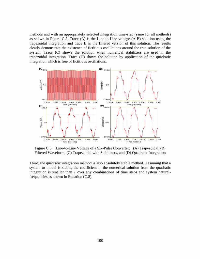
190

methods and with an appropriately selected integration time-step (same for all methods)

as shown in Figure C.5. Trace (A) is the Line-to-Line voltage (A-B) solution using the

trapezoidal integration and trace B is the filtered version of this solution. The results

clearly demonstrate the existence of fictitious oscillations around the true solution of the

system. Trace (C) shows the solution when numerical stabilizers are used in the

trapezoidal integration. Trace (D) shows the solution by application of the quadratic

integration which is free of fictitious oscillations.

2.939 2.948 2.958 2.967 2.976 2.986 2.995 2.939 2.948 2.958 2.967 2.976 2.986 2.995

2.939 2.948 2.958 2.967 2.976 2.986 2.995 2.939 2.948 2.958 2.967 2.976 2.986 2.995

Time (Second) Time (Second)

Time (Second) Time (Second)

196.0

0.0

-196.0

196.0

0.0

-196.0

8.91

0.0

-8.91

Vol

tage

(M

V)

Vol

tage

(kV

)

Vol

tage

(K

V)

Vol

tage

(K

V)

(A) (B)

(C) (D)

196.0

0.0

-196.0

Figure C.5: Line-to-Line Voltage of a Six-Pulse Converter: (A) Trapezoidal, (B)

Filtered Waveform, (C) Trapezoidal with Stabilizers, and (D) Quadratic Integration

Third, the quadratic integration method is also absolutely stable method. Assuming that a

system to model is stable, the coefficient in the numerical solution from the quadratic

integration is smaller than 1 over any combinations of time steps and system natural-

frequencies as shown in Equation (C.8).

191

Appendix D: Reliability Model Parameters

This appendix provides the symbols and typical values of component reliability

parameters. The list shows all the components that appear in the 8 wind farm

configurations discussed above. These parameters are used for the example calculation of

the 8 configurations provided in the previous subsections.

Table D.1: Reliability Parameters of Components

Icon

Component Failure Rate

Typical Value of Failure Rate

Repair Rate

Typical Value of Repair Rate

Wind Turbine

Small Switch 0.0061

Small

Transformer 0.003

Small AC/DC

Converter =3.233

Large AC/DC

Converter =3.233

In Farm AC

Transmission Line

0.0189

In Farm DC

Transmission Line

Large Switch

AC Bus

DC Bus

DC/AC

Converter 3.233

20 Hz

Transformer 0.0032

DC

Transmission Line

3.04

192

Table D.1: Reliability Parameters of Components (continued)

20Hz AC

Transmission Line

Cyclo Conveter

60Hz AC

Transmission Line

3.04

Large/

Substation Transformer

20Hz Inter-

Transmission Line

=

60Hz Inter-

Transmission Line

=

193

Appendix E: Cost Parameters

This appendix provides the typical values of individual acquisition cost for the

components in the configurations. The list shows all the components that appear in the 8

wind farm configurations discussed above. These parameters are used for the example

calculation of the 8 configurations provided in the previous subsections. It should be

noted that the acquisition cost of one type of component, such as wind turbine, is

different in different kV levels. For example, the wind turbine operating at 25 kV is more

expensive than the turbine operating at 13.8 kV. Table E.1 only provides a typical

acquisition cost of the components operating at 13.8 kV.

E.1: Typical Acquisition Cost of Components in the 8 Configurations

Component Typical Acquisition Cost ($)

Wind Turbine 1000,000

Small Switch 300

Small Transformer 5000

Small AC/DC Converter 2000

Large AC/DC Converter 30,000

In Farm AC Transmission Line 500

In Farm DC Transmission Line 500

Large Switch 5000

AC Bus 1000

DC Bus 1000

DC/AC Converter 20,000

20 Hz Transformer 20,000

DC Transmission Line 2000


Cyclo Conveter 5000


Large/ Substation Transformer 50,000

20/60 internal transmission line 1000

Table E.2 provides the data of cost of transmission lines, which is the mean per-mile cost

of the lines.

194

E.2: Cost of Transmission Lines

Voltage (kV) Range of per-mile Costs

(k$)

Mean per-mile Cost from

Composite Database (k$)

13.8 41 - 50 44

34.5 43 – 55 48

46 46-56 49

69 60 – 238 107

115 91 – 228 124

138 96 – 308 165

161 105 – 333 182

230 129 – 371 235

345 218 – 503 341

500 364 – 972 519

765 Extrapolated 782

Based on flat terrain. Does not include land, environmental, planning, or construction

supervision costs.

Documents

Low Frequency Transmission - Power Systems Engineering