Low-Frequency Fluid Waves in Fractures and Pipes

Valeri Korneev

Lawrence Berkeley National Laboratory, Berkeley, CA 94720

ABSTRACT

Low-frequency analytical solutions have been obtained for phase velocities of

symmetrical fluid waves within both an infinite fracture and a pipe filled with a viscous fluid.

Three different fluid wave regimes can coexist in such objects, depending on the various

combinations of object parameters. These regimes include Biot, Stoneley, and “narrow

channel.” Equations for velocities of all these regimes have explicit forms and are verified by

comparisons with exact solutions. Computations suggest that for pipes, the most common is

the Biot regime, while for fractures it is the Stoneley regime. For real rock in fractures, the

Biot regime exists only when fluid is in a gaseous state. The dominant role of fractures in rock

permeability at field scales and the strong amplitude and frequency effects of Stoneley guided

waves suggest the importance of incorporating these effects within poroelastic theories.

INTRODUCTION

We consider and compare propagation of a fundamental symmetrical mode (wave) for two

model geometries: a fracture and a pipe, both infinite along the symmetry axis, filled with

viscous fluid, and surrounded by an unbounded elastic medium. The importance of this fluid

wave is a well established fact for boreholes (tube wave) and supported by recent numerical

modeling results for fractures (Korneev et al, 2009; Feihner and Schmalholz, 2009; Derov et

al., 2009; Bakulin et al, 2008), indicating the dominant role of this wave in wave propagation.

In Korneev (2008), it was found that in fractures filled with viscous fluid, a fluid wave can

propagate in both the Stoneley guided wave (Paillet and White, 1982) and the Biot slow wave

(Biot, 1956ab) regimes. For both of these regimes, the fluid wave is dispersive, but its

dependence on model parameters is significantly different. While in the Biot regime the

dispersion exists only in viscous fluids and does not depend on wall elastic parameters, the

Stoneley guided wave is dispersive, even for zero fluid viscosity, and depends on the wall’s

shear modulus. Relationships between these two regimes remained unclear: What are the

conditions of their existence? What is the difference between fractures and pipes in fluid wave

propagation? Hereafter, we refer to a channel when addressing fluid-containing parts for both

geometries, which is a useful notation for discussion of similarities and differences between

them. In this paper, we obtain such conditions for the abovementioned regimes and show that

at a limit of small channel thickness, there also exists a diffusive narrow channel propagation

regime, which differs from the Biot regime in its dependence on model parameters.

THEORY FOR A FRACTURE

Previous Work

The Stoneley guided wave, which propagates in a fluid layer bounded by elastic walls,

was first obtained as a mathematical result by Krauklis (1962). Paillet and White (1982) re-

derived this solution when comparing waves in a borehole and its 2D analog. Their solution

has an implicit form as a fundamental symmetric mode that propagates along the fracture with

a velocity that approaches zero at zero frequency. Ferazzini and Aki (1987) applied this

solution to explain low-frequency tremors observed before volcanic eruptions.

2

Fluid-filled fracture waves also have been investigated both numerically and in laboratory

studies to explain volcanic tremors and monitoring of hydraulic fracturing (Chouet, 1986,

1988; Ferrazzini et al., 1988; Tang and Cheng, 1988; Goloshubin, et al., 1994; Groenenboom

and Falk, 2000; Groenenboom and van Dam, 2000; Groenenboom and Fokkema, 1998), Slow

fluid waves are essential for generating tube-wave reflections from intersecting fractures

(Hornby et al., 1989; Kostek et al., 1998 a, b; Derov et al., 2009; Ziatdinov et al., 2006). The

high amplitudes of such waves make the solution of relevant problems rather simple, because

we can ignore most other types of waves without compromising the result. The energy-

trapping ability of such waves illustrates the distinctive feature of fluid-filled fractures,

specifically their waveguide-like capability of transporting energy. Propagation of the

Stoneley guided waves in a fracture filled with viscous fluid was described in Korneev (2008).

In the latest developments regarding the subject, Frehner and Schmalholz, (2009) modeled

these waves for intersecting fractures using a finite-element method, and Korneev et al. (2009)

compared analytical results with those obtained using OASES software.

Fluid Waves in a Fracture

Here, we consider all low-frequency symmetrical fluid waves using the results from

Korneev (2008), but change some notations to make them uniform with a similar problem for

a cylindrical pipe—also a subject of this paper. A symmetric model consists of the

layer 2h z h 2 , filled with viscous fluid between two homogeneous elastic half-spaces

comprised of the same material. (We provide only the necessary expressions here; more

details can be found in Korneev [2008].) The index 1j indicates the parameters and fields

3

related to the viscous fluid layer, while index 2j indicates the values related to elastic half-

spaces.

In both media, the relations between the body wave velocities and media parameters are

the same: a longitudinal (P-) wave propagates with velocity

2j jPj

j

V

(1)

and a shear (S-) wave with velocity

jSj

j

V

, (2)

expressed through Lame constants j , j and density j ( 1, 2j ) . We assume that

2 2 1P SV V V P , which is the most common case for rocks at depth.

The linearized equation of motion for compressible viscous fluid takes the form (Korneev,

2008):

22

2

10

3 Pf f

ct t t

2 u u u

u , (3)

with time t, fluid density 1f , viscosity coefficients , , and speed of sound for the

zero-viscosity limit.

pc

Using the time dependence of the fields in the form exp( )i t , with angular frequency ,

equation 3 describes the propagation of dissipating P- and S- waves with complex velocities:

2P1

4

3Pf

V c i

, (4)

1Sf

iV

, (5)

4

and complex Lame constants:

21

2

3P fc i

, (6)

1 i . (7)

We seek a solution in the form of a surface wave with wavenumber vx

f

k

, propagating

along the OX axis with phase velocity v f .

Velocities in both media have corresponding wavenumbers:

/Pj P j /Sj Sjk Vk V , . (j=1,2). (8)

Continuity conditions for two components of both stress and displacement at the

boundaries lead to four linear equations for coefficients of those components. The

dispersion equation for symmetric modes is obtained by finding values of

/ 2z h

v f for which the

determinant

2 2 21 1 2 2 2 1 1 2 1 1(1 ) ( ) ( )( ) ( )s p s x x x x pc k b c ic k a k b k 2s

2 2 2 22 2( ) ( )x x p s xk k ac k ca b 0 (9)

of the system is zero, where

1 1 1=i tanh2P P

hi

, (10)

1 1 1=i coth2S S

hi

, (11)

2 2Pj Pjk h z , 2 2

sj sjk h z , ( j=1,2) (12)

and coefficients a, b, and c have expressions

5

2

21

v(1 )

2f

xS

a kV

, 2

22

v(1 )

2f

xS

b kV

, 1

2

c

. (13)

In equation 9, the factor in square brackets is exactly that of equation 23 from Korneev

(2008). The factor 1S in equation 9 gives an extra root for the fluid wave propagating with

the (rather small) velocity of the shear wave in viscous fluid given by equation 5. Low-

frequency approximation means that both frequency and thickness h are small enough to

provide the conditions

1 12P

h , 2 12P

h and 2 12S

h , (14)

which reduce the equation for the roots of the square brackets factor in equation 9 to

2 2

1 2 2 21 2 2

v vk (1 ) 2

(1 )f f f

xP S

hV V

. (15)

Approximating in Equation 15 the function 11 by the truncated Taylor series of the coth

function

22 2x

1 2x 1

vk21

k 12f

S

h

h V

, (16)

we get the cubical polynomial equation

3 3 23 20 0 0

2 2 20

v vS S Bf f

P P B

V V V

V V V0

, (17)

for determining v f .

Equation 17 contains three parameters, all of which are velocities with the forms (Korneev,

2008):

1. (18)

1

322

0 (1 ) ,Sf

hV

6

(A low-frequency Stoneley wave velocity in a fracture filled with non-viscous fluid, where

2 2/S PV V );

2. 0 1fr f

B P

iV V

, (19)

(A low-frequency fluid wave velocity in a fracture with rigid walls (Biot regime),

where is fracture permeability; and 2 /12fr h

3. 1P PV V , (20)

(a P-wave velocity in the fluid from equation 4. Equation 17 has three roots, which can be

explicitly found using the Cardano formula (Abramowitz and Stegun, 1972). Among these

three roots, only one has a positive real part and therefore describes a physical wave.

However, the structure of equation 17 allows for finding its asymptotic solutions in a

straightforward way.

If the second term in equation 17 is much smaller than the first term, then

203

0 2 20

v Bf S S

P B

VV V

V V

. (21)

and

302

SS

P

VV

V (22)

which after simple algebra is equivalent to

SV V B , (23)

If in Equation 21,

2 2P BV V , or

2

1 fr f h

S

, (24)

7

where viscous skin

12

f

S

(25)

is much smaller than fracture thickness, the elastic forces dominate viscous ones and fluid

wave

0v 13

fr ff S

iV

, (26)

propagates in the Stoneley regime. This regime exists for “thick” fractures and/or low fluid

viscosity.

If in Equation 21,

20

2P BV V , or

2

1h

S

, (27)

then viscous forces are taking over, and

2 22233

2v

12B

f SP

VV h i

V

(1 )

, (28)

which was called a “thin” fracture regime in Korneev (2008), or a “narrow channel” regime

of the fluid wave.

If in equation 17, the second term dominates over the first term, then

0

2 20

v P Bf B

P B

V VV

V V

. , (29)

and such term relationships mean that

302

SB

P

VV

V , (30)

which is equivalent to

8

SV V B , (31)

exactly the opposite result of inequality 23.

At low frequencies (inequalities 27) equation 29 gives

0 1v fr ff B P

iV V

, (32)

which is a propagation in a Biot regime, when interaction of the fluid wave with the fracture

walls occurs exclusively through viscous friction forces.

At high frequencies, (inequalities 23), equation 29 gives

v f PV , (33)

which is a propagation of body P-waves in the fluid.

Inequalities 23 and 31 mean that for any parameter set, a wave propagation regime

corresponds to a regime with the slowest velocity. The regime change occurs when

SV V B (34)

Thus, when

SV V P , (35)

the wave propagates with the velocity of P- waves in the fluid (equation 33). If both and

are less than

SV

0BV PV then, after substitution of expressions 21 and 29 into equation 34, we

obtain

22 3

22

1 6 6

(1 )f P

Tf f

V

h h h

(36)

for a transitional frequency T that separates different propagation regimes.

9

For thick fractures and small viscosities, when

22 3

22

16 (1 )

f Ph V

(37)

a transition between Stoneley and Biot regimes takes place, and equation 36 becomes

3

22 (1 )

f P

T

V

h

(38)

If the inequality sign in 37 is reversed, then

31

2 2212 (1 )T

2, (39)

and the transition occurs between the Biot and narrow channel regimes.

NUMERICAL RESULTS FOR A FRACTURE

Numerical study of fluid waves in a fracture involved comparison of obtained exact and

asymptotic solutions for a set of media models with different parameters. The exact solution

was obtained by a direct root search when left hand side of the equation 9 was computed on a

dense grid for complex velocity v f . Both the real and imaginary parts varied in the range

from zero to a value exceeding velocity in the fluid. The computed function was analyzed

numerically always revealing the presence of two roots. One of the roots corresponded to

velocity of shear waves in the fluid. The other root numerically coincided with the only

physical solution of equation 17 which was computed using Cardano formulas. Among three

roots of equation 17 just one has a positive real part giving only physically interpretable

estimate for the exact solution of equation 9. The asymptotic solutions 21, 28 and 29 were

10

compared with the exact solution. For all examples presented here, the parameters of the

elastic medium are m/s, m/s. and g/cm3. Figure 1 shows real

phase velocities as the functions of density. The parameters of the model are m/s,

the viscosities

P2 5000V S2 3000V 2 2.7

1500Pc

Pc

1 cP, frequency 20 Hz, m/s and the fracture thickness is 10-3

m. At low densities the exact solution follows the solution for the Biot regime, while at

higher densities it follows the Stoneley regime. Note, that the transition between these two

regimes corresponds to the conditions for inequalities 23 and 31. Figure 2 shows phase

velocities as function of frequency for when fluid has same parameters as the “air” at

atmospheric pressure, when m/s,

1500P

0.0013

c

f330 g/cm3, 0.01 cP. Here the exact

solution accurately follows the Biot regime solution. However, for 10 times thinner fracture

(h=10-4 m.) the narrow channel regime takes place at low frequencies (Figure 3). Case when

air is compressed at 100 atm of hydrostatic pressure (approximately at 1 km depth) is shown

on Figure 4, where 0.13f g/cm3 and h=10-3 m. For this set of parameters the dispersion

curve belongs to a transition between the Stoneley regime (equation 21) and the high

frequency solution (equation 33). Water-filled fracture case with m/s, 1,500Pc

1.0f g/cm3, 1 cP and h=10-3 m. is shown on Figure 5. Results for oil-filled fracture

where all the parameters have the same values as for Figure 6, except viscosity 10 cP

are shown on Figure 6. For seismic range of frequencies the solutions for both water and oil

are well represented by Stoneley regime.

We will discuss these results together with similar results for a pipe which is the

subject of the next section.

11

THEORY FOR A PIPE

Previous Work

Fluid-filled boreholes are one of the most important signal-carrying channels in

prospecting geophysics, and the literature on the properties of borehole fluid waves is quite

extensive (White, 1983; Burridge et al, 1993, Schoenberg et al 1981, Cheng and Toksoz,

1981; Chang et al, 1988; Haddon, 1989, Norris, 1989, etc). Tube waves are used for

permeability logging, fracture detection, reservoir monitoring, and borehole integrity testing.

The similarity of Stoneley (tube) and Biot slow waves has been noted (Chang et al, 1988);

Norris (1987) even described the tube wave as “a limiting case of the Biot slow wave.” In

poroelastic theory (Biot, 1956b), it is assumed that on a pore scale the channel walls are rigid,

and that a fluid wave in a cylindrical pipe is a core model for fluid-solid interaction. In reality,

however, values of liquid rigidity are comparable with those of elastic rocks, and therefore

wall-rigidity assumptions needs to be evaluated, as was done for the case of fractures in the

previous section. Here we revisit the problem of low-frequency wave propagation in a

cylindrical pipe filled with viscous fluid and demonstrate the existence of a “narrow channel”

regime at nanoscale levels, in addition to the Biot and Stoneley low-frequency regimes.

Fluid Waves in a Pipe

We are interested in the low-frequency properties of purely symmetric fluid waves

propagating along a thin cylindrical well (or a pipe) filled with viscous fluid. Outside of the

cylinder with radius R, the medium is elastic. In the following, index 1j refers to fluid,

while index 2j denotes the elastic medium. Here, we also use notations introduced in

equations 1–8.

12

It is assumed that longitudinal (P-) and shear (S-) waves in both media of the pipe satisfy

welded boundary conditions at the pipe wall, providing continuity for stresses and

displacements. (Mathematical formalism and the main expressions for wave propagation

problems with cylindrical symmetry are presented in Appendix A.) The pure symmetry of the

problem leaves only m=0 in the field expansions. As a result, the propagation velocities v f of

the fluid waves can be found as the roots of the determinant

1 1 2 2

1 22 2 2 2

1 1 1 1 1 2 2 2 2 21

2 2 2 21 1 21 1 1 1 1 1 2 1 2 2

1 1 2 2

2 (2 ) 2 (2 0

2 (1 ) 2 (1 ) 2 (1 ) 2 (1 )

z z

z s z s

z s z z s zs

p p z p p zp s p s

k k

k k

k k k

k k k kR R R

2

)k

R

(40)

Velocity v f is directly related to propagation wave number through the expression zk

v fzk

, parameters ,Pj Sj are defined through the formulas

2pj pj zk k 2 , 2 2

sj sjk k z j=1,2, (41)

and the functions 1 , 1 , 2 , and 2 have the expressions

1 11

0 1

( )

( )p

p

J R

J R

, 1 1

10 1

( )

( )s

s

J R

J R

, (2)

1 22 (2)

0 2

( )

( )p

p

H R

H R

,

(2)1 2

2 (2)0 2

(

( )s

s

H

H R

)R

, (42)

where is the Bessel function, and is the Hankel function of the second kind. ( )kJ Z (2) ( )kH Z

For small arguments, 1Z , the following asymptotic expressions

21

0

( )(1 )

( ) 2 8

J Z Z Z

J Z ,

(2)1(2)0

( ) 1

( ) ln( 2)

H Z

H Z Z Z (43)

can be used.

13

Low-frequency assumption means that

1 1p R , 2 1p R , 2 1s R , (44)

and the asymptotic expressions 43 can be applied to equation 40. This reduces Equation 40 to

2 2 2 21 12 21

1 2 2 1 1 1 1 21

2(1 ) (1 ) 0

8 8p p

s z ps

R Rk k

R

. (45)

Note that according to the equations 42, the ratio 1

1

2

s R

from equation 45 has a limit equal to

one if the argument of 1 goes to zero.

Factor 1s gives equation 45 an immediate solution:

1 1v vf sf

i

, (46)

which is the same as in the fracture case.

At higher frequencies, when

1 1s R , (47)

the argument for 1 is large, and 1 i , equation 45 becomes

22 21 1 1 2 1 22 2

1

( ) ( )2

zp z

s z

k Ri k k

k k

0 , (48)

which can be put in a form of a cubic polynomial with respect to , and solved explicitly

using Cardano formulas. For the small viscosity

2zk

, the expression in square brackets must

approach zero, and we obtain

1 21

1 1 2

v vf p

, (49)

which for zero viscosity gives

14

21

1 2

v vf p

, (50)

the velocity of the Stoneley (tube) wave (White, 1965) propagating along a well filled with

fluid.

When 1 1s R , then approximation 43 can be used for 1 , and leads to the following

quadratic equation with respect to 2zk

21 1 1 22

2 2 22 1 1 1

8 ( )

( 2 )p

zs p

kk

R k k

(51)

Introducing a dimensionless real parameter

22

28fR

p

(52)

that determines the main component in the denominator of equation 51, we find that when

, then the module of the square of the coefficient for is much larger than the module

of the last term. Thus, for from equation 51, we obtain

1p 2zk

1p

22 1

1 2

v v c ff p

i

, (53)

where 2

8c

R is pipe permeability. This wave has a velocity close to that of the Biot wave

(Appendix B) for a cylinder with the “Stoneley” correction factor 2

1 2

. If the rigidity of

the fluid goes to zero, then 2v f (equation 53) approaches the Biot regime solution (Appendix

B) for the slow wave in a pipe.

When

15

1c f

(54)

the fluid wave velocity becomes undispersive and propagates as a tube wave described by

equation 50.

When 1p (small pipe radius), then the second term in equation 51 can be neglected, and

we have

2 11 2

v vf p

i

i

, (55)

which describes the “narrow channel” propagation regime in the pipe.

Equations 46, 53 and 55 describe propagation of the diffusion waves.

NUMERICAL RESULTS FOR A PIPE

The main idea behind the numerical study of a pipe is the same as for the case of a

fracture, which requires evaluating the validity of different propagation regimes for realistic

rock parameters. The exact solution was obtained by the direct root search of equation 40,

which, similarly to the fracture case, revealed the existence of two roots. One of the roots

(equation 46) corresponds to the velocity of shear waves in the fluid. The other root represents

the symmetric fluid wave, which propagates in different regimes depending on parameters

values. For all data presented here m/s, m/s,, m/s,

g/cm3 and fluid viscosity

1500Pc P2 1800V S2 800V

2 2.7 10 cP (oil). Figure 7 shows the phase velocities for

a pipe as a function of the pipe radius R for 20 Hz frequency. Also shown are: , the

solution for the Stoneley regime (equation 49) , the solution for the general Biot regime

(Equation 53), and the solution for “narrow channel” regime (equation 55). Figure 8 shows

P1V

16

phase velocities as a function of frequency for a “thick” pipe with 10-4 m radius, while Figure

9 presents computations for a “thin” pipe with 10-8 m radius.

DISCUSSION

Theoretical and numerical results presented in this study reveal several similarities in

wave propagation between fracture and pipe. The fluid symmetrical wave is always present in

the solution, and it can propagate in different regimes including Stoneley, Biot and “narrow

channel” regimes. The last regime occurs at very small scales, when channel width is much

smaller than skin depth. This regime takes the form of equation 28 for a fracture and equation

55 for a pipe. Velocities of these waves directly depend on the shear modulus of walls, fluid

viscosity, and frequency, and therefore wall elasticity is an important parameter here. These

waves propagate by squeezing in fluid through the narrow channels of fractures and pipes. An

extra fluid wave propagating with the velocity of a shear wave in the fluid always exists at

low frequencies. It has a diffusion type of propagation and quickly dissipates. This is a

generally a rather slow wave, but it can be faster than the other fluid wave, depending on the

parameters.

The relationship of solutions representing both the Biot propagation regime and the Biot

slow wave in poroelastic theory follows from the similarity in asymptotic expressions for

these waves at low frequencies, as well as from assumptions used for deriving dynamic

poroelastic equations. Section 2 of Biot (1956b) considers the oscillatory flow of fluid

between two rigid parallel walls, which is the same problem for the Biot solution in an

infinitely-stiff fracture considered in Korneev (2008) using a somewhat different technique.

Section 3 of Biot (1956b) solves the analogous problem for a cylindrical tube (see Appendix

17

C). Then, Biot calculates a friction force acting between fluid and elastic skeleton using “the

assumption that the variation of friction with frequency follows the same laws as found in the

foregoing for the tube of uniform cross section” (page 182). Therefore, at pore scale, the

elasticity of pore walls in Biot’s theory is neglected, and it operates on a macro level only,

where the effects of numerous pores are evaluated. At low frequencies, the solutions for the

Biot slow wave (equation C1), and Biot regimes for the fracture (equation 32) and a pipe

(Equation 53) have the same dependence on frequency, permeability, and fluid viscosity, in

the form

f

iV V

(56)

where V is some velocity not dependent on any parameters under the radical, is

permeability of the porous media, 2

12

h for a fracture, and 2

8

R for a pipe. However, in

the two latter cases, the Biot regime transfers into narrow channel regimes at the low

frequency limit.

A Stoneley wave propagation regime is very different for the considered geometries. In a

pipe with a large radius (or in absence of viscosity) at low frequencies, the Stoneley wave has

virtually no dispersion propagating as a tube wave. By contrast, in a fracture, the Stoneley

guided wave has a strong dispersion. In a pipe, the Stoneley wave regime converts to a Biot-

wave regime quite rapidly, as soon as the condition

1c f

(57)

is valid. (Strictly speaking, the wave described by equation 53 is not quite a Biot wave

because of the Stoneley correction factor.). In a fracture, the Biot wave regime can be

18

achieved for severely contracting cases only when fluid is in a gaseous state. A quite common

derivation of the Biot solution occurs when the rigidity of the walls is placed at infinity (e.g.,

Chang et al., 1988). Such an assumption cannot be justified from the physical point of view.

Indeed, common densities and shear-wave velocities for known rocks differ from density and

sound wave velocity in water by a factor of 2–3, which is far from the high-contrast

assumption between the channel walls and the fluid. Such a contrast can be achieved by

applying the theory to a gas only, but this restriction is too severe for poromechanic

applications.

Besides having some aforementioned similarity, the narrow channel regimes described by

equations 28 and 55 differ in their dependence on fluid viscosity is different. In a fracture,

this regime starts relatively quickly as the fracture thickness decreases, while for realistic

parameters in pipes, it takes place surprisingly at nanoscale level at seismic frequencies.

Moreover, for liquids, wall rigidity is always a factor affecting wave propagation.

The considered problems had just one fluid-channeling element, which is taken as infinite

in one or two directions. Real rocks contain a wide variety of pores and fractures that can

intersect, and are distributed in sizes and shapes that provide conditions for different fluid

wave regimes. The fractal character of fracture and pore distribution in real rock suggests a

rapid increase of their numbers for decreasing scales Diffusion waves are slow and propagate

short distances, but both the numerousness of small-scale channels and reflection-refraction

on heterogeneities, where diffusion waves can directly impact boundary conditions, can

possibly make significant contributions to overall wave propagation. (Accurate consideration

of all wave propagation effects in such media is a very complex problem, which is beyond of

a scope of this study.)

19

The hydrogeology results provide strong evidence that fractures play a key role in rock

permeability. Permeability was measured for a wide range of scales in a number of

comprehensive studies for a variety of geologic environments (Clauser, 1992; Neuman, 1994;

Shultze-Makuch et al., 1999; Shultze-Makuch and Cherkauer, 1998; and Gelhar, 1993).

Typically, five-orders-of-scale increase corresponds to 5–7 orders of permeability increase,

suggesting the dominant role of fractures in fluid flow at field scales.

This study does not directly address the attenuation of fluid waves in channels. This is for

several reasons. Such attenuation in fractures was computed and discussed in Korneev (2008)

and Korneev et al. (2009). In Biot and narrow channel regimes, wave propagation describes

diffusion processes that have well-known attenuation processes. General low frequency

asymptotics representing solutions of cubical polynomials 17 and 39 have explicit forms and

allow a simple computation of complex velocities (and, therefore, attenuation) for any chosen

parameter set.

CONCLUSIONS

Analytical solutions have been obtained for the phase velocities of fluid waves within both

an infinite fracture and a pipe filled with a viscous fluid at low frequencies. Two fluid waves

can co-exist in such objects: diffusive wave propagating with shear-wave velocity in the fluid,

and a general fluid wave that can propagate in different regimes depending on object

parameters. These include Biot, Stoneley, and “narrow channel” wave regimes. Computations

for realistic rock parameters suggest that for pipes, the most common regime is the Biot slow

wave, while for fractures. it is the Stoneley (guided) wave.

20

ACKNOWLEDGMENTS This work was supported by the the U. S. Department of Energy under Contract No. DE-AC02-05CH11231. Andrey Bakulin, Dmitry Silin, Gennady Goloshubin, German Maximov and an anonymous reviewer have made many helpful comments.

REFERENCES

Abramowitz, M. and Stegun, I. A. , 1972, Handbook of Mathematical Functions with

Formulas, Graphs, and Mathematical Tables, New York: Dover.

Burridge, R., S. Kostek, and A. L. Kurkjian, 1993, Tube waves, seismic waves, and effective

sources: Journal of the Acoustical Society of America,. 93, 2396-2396.

Biot, M.A., 1962, Mechanics of deformation and acoustic propagation in porous media:

Journal of Applied Physics, 33, 1482–1498.

Biot, M.A., 1956a, Theory of propagation of elastic waves in a fluid-saturated porous solid. I.

Low-frequency range: Journal of the Acoustical Society of America, 28, 168–178.

Biot, M.A., 1956b, Theory of propagation of elastic waves in a fluid-saturated porous solid. II.

Higher frequency range: Journal of the Acoustical Society of America, 28, 179–191.

Castagna, J.P., Sun, S., and S.R. Wu., 2003, Instantaneous spectral analysis: detection of low-

frequency shadows associated with hydrocarbons: The Leading Edge, 22, 120-127.

Chang, S.K., Liu, H.L. and D.L. Johnson, 1988, Low-frequency tube waves in permeable

rocks: Geophysics, 53, 519-527.

Cheng, C.H. and M.N. Toksoz, 1981, Elastic wave propagation in a fluid-filled borehole and

synthetic acoustic logs: Geophysics, 46, 1042-1053.

21

Chouet, B., 1988, Resonance of a fluid-driven crack: Radiation properties and implication for

the source of long-period events and harmonic: Journal of Geophysical Research., 93, 4375-

4400.

Chouet, B., 1986, Dynamics of a fluid-driven crack in three dimensions by the finite-

difference method: Journal of Geophysical Research., 91,, 13967–13992.

Clauser, C., 1992, Permeability of crystalline rocks: Eos Transactions, American Geophysical

Union, 73, 233.

Derov, A, Maximov, G., Lazarkov , M. , Kashtan, B., and A. Bakulin, 2009, Characterizing

hydraulic fractures using slow waves in the fracture and tube waves in the borehole, 79th

Annual International Meeting, SEG, Expanded Abstracts. .

Dutta, N.C. and H. Ode, 1979, Attenuation and dispersion of compressional waves in fluid-

filled porous rocks with partial gas saturation (White model) – Part I: Biot theory,

Geophysics, 44, 1777-1788.

Ferrazzini, V., Chouet, B., Fehler, M. and K. Aki,, 1990, Quantitative analysis of long-period

events recorded during hydrofracture experiments at Fenton Hill, New Mexico: Implications

for volcanic tremor: Journal of Geophysical Research, 95, 21,871-21,884.

Ferrazzini, V., and K. Aki, 1987, Slow waves trapped in a fluid-filled infinite crack:

Implications for volcanic tremor, Journal of Geophysical Research, 92, 9215–9223.

Frehner, M. and S. Schmalholz, 2009, Finite-element simulations of Stoneley guided wave

reflection and scattering at the tips of fluid-filled fractures: Geophysics, in print.

Gelhar, L. W., 1993, Stochastic Subsurface Hydrology, Prentice-Hall, Old Tappan, N. J.

22

Goloshubin, G.M., Korneev V. A., Silin, D. B., Vingalov V.S. and C. VanSchuyer, 2006,

Reservoir imaging using low frequencies of seismic reflections: The Leading Edge, 25, 527-

531

Goloshubin G.M., Krauklis P.V., Molotkov L.A., Helle H.B., 1994, Slow wave phenomenon

at seismic frequencies: 63th Annual International Meeting, SEG, Expanded Abstracts,

809-811.

Groenenboom, J. and J. Falk, 2000, Scattering by hydraulic fractures: Finite-difference

modeling and laboratory data: Geophysics, 65, 612–622.

Groenenboom, J., and D. B. van Dam, 2000, Monitoring hydraulic fracture growth:

Laboratory experiments: Geophysics, 65, 603–611.

Groenenboom, J., and J. T. Fokkema, 1998, Guided waves along hydraulic fractures,: 67th

Annual SEG Meeting.

Haddon, R.A.W., 1989, Exact Green’s functions using leaking modes for axisymmetric

boreholes in solid elastic media: Geophysics, 54, 609-620.

Hornby, B. E., Johnson, D. L.,Winkler, K.W., and R. A. Plumb, 1989, Fracture evaluation

using reflected Stoneley-wave arrivals: Geophysics, 54, 1274–1288.

Korneev, V., A. Ponomarenko, and B. Kashtan, 2009, Stoneley guided waves: What is

missing in Biot’s theory?: Proceedings of the Forth Biot Conference on Poromechanics:

DEStech Publication Inc., 706-711, ISBN 978-1-6059-5006-8.

Korneev, V., 2008, Slow waves in fractures filled with viscous fluid: Geophysics, 73,

doi10.1190/1.2870081.

Korneev, V. A., Goloshubin, G. M., Daley, T.V., and Silin, D.B., 2004, Seismic low-

frequency effects in monitoring of fluid-saturated reservoirs, Geophysics, 69, 522-532.

23

Kostek, S., Johnson, D. L., and C. J., Randall, 1998, The interaction of tube waves with

borehole fractures. Part I: Numerical models: Geophysics, 63, 800–808.

Kostek, S., Johnson, D.L., Winkler, and B. E. Hornby, 1998, The interaction of tube waves

with borehole fractures, Part II: Analytical models, Geophysics, 63, 809–815,

Krauklis, P. V., 1962, About some low frequency oscillations of a liquid layer in elastic

medium: Prikladnaya Matematika i Mekhanika, 26, 1111-1115 (in Russian).

Landau, L.D., and E.M. Lifschitz, 1959, Fluid Mechanics: Reading, MA, Pergamon Press.

Neuman, S. P., 1994, Generalized scaling of permeabilities: Validation and effect of support

scale, Geophysical Research Letters, 21, 349–352.

Norris, A., 1989, Stoneley wave attenuation and dispersion in permeable formations:

Geophysics, 54, 330-341.

Norris, A., 1987, The tube wave as a Biot slow wave, : Geophysics, 52, 694-696.

Paillet, F.L. and J.E. White, 1982, Acoustic models of propagation in the borehole and their

relationship to rock properties: Geophysics, 47, 1215–1228.

Schoenberg, M., T. Marzetta, J. Aron, and R.P. Porter, 1981, Space-time dependence of

acoustic waves in a borehole: Journal of the Acoustical Society of America, 70, 1496-1507.

Roever, W.L., J.H. Rosenbaum, and T.F. Vining, 1974, Acoustic waves from an impulsive

source in a fluid-filled borehole: Journal of the Acoustical Society of America, 55, 1144-1157.

Schulze-Makuch, D., and D. S. Cherkauer, 1998, Variations in hydraulic conductivity with

scale of measurements during aquifer tests in heterogeneous, porous carbonate rock

Hydrogeology Journal, 6, 204–215.

Schulze-Makuch, D., D. A. Carlson, D. S. Cherkauer, and P. Malik, 1999, Scale dependency

of hydraulic conductivity in heterogeneous media: Ground Water, 37, 904–919.

24

Tang, X. M. and C. H. Cheng, 1988, Wave propagation in a fluid-filled fracture – an

experimental study: Geophysical Research Letters, 15, 13, 1463-1466.

White, J. E., 1965, Seismic waves: Radiation, transmission, and attenuation: McGraw-Hill

Book Co.

Ziatdinov, S., Bakulin, A. and B. Kashtan, 2006, Tube waves from a horizontal fluid-filled

fracture of a finite radius: 76th Annual International Meeting, SEG, Expanded Abstracts, 369-

372.

25

FIGURES

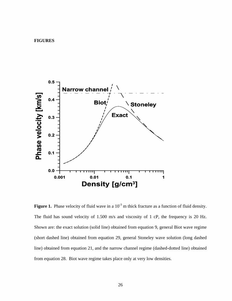
Figure 1. Phase velocity of fluid wave in a 10-3 m thick fracture as a function of fluid density.

The fluid has sound velocity of 1.500 m/s and viscosity of 1 cP, the frequency is 20 Hz.

Shown are: the exact solution (solid line) obtained from equation 9, general Biot wave regime

(short dashed line) obtained from equation 29, general Stoneley wave solution (long dashed

line) obtained from equation 21, and the narrow channel regime (dashed-dotted line) obtained

from equation 28. Biot wave regime takes place only at very low densities.

26

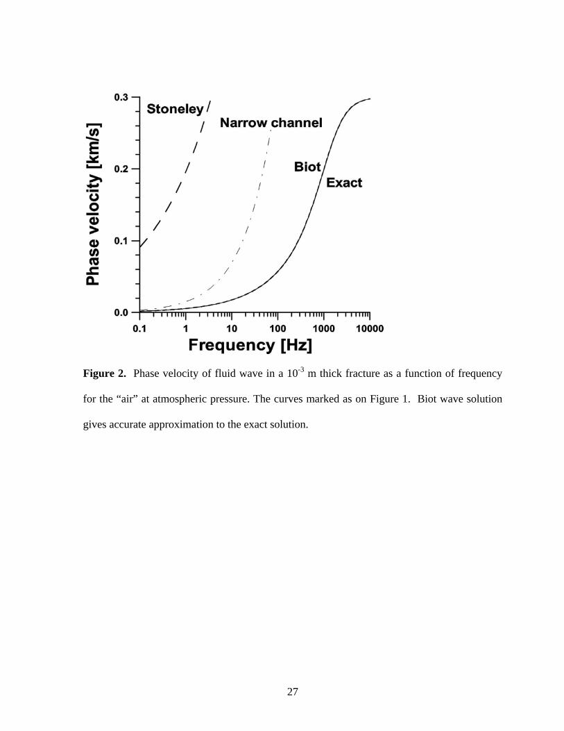
Figure 2. Phase velocity of fluid wave in a 10-3 m thick fracture as a function of frequency

for the “air” at atmospheric pressure. The curves marked as on Figure 1. Biot wave solution

gives accurate approximation to the exact solution.

27

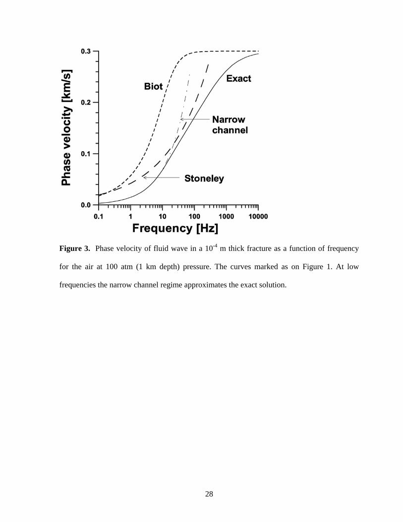
Figure 3. Phase velocity of fluid wave in a 10-4 m thick fracture as a function of frequency

for the air at 100 atm (1 km depth) pressure. The curves marked as on Figure 1. At low

frequencies the narrow channel regime approximates the exact solution.

28

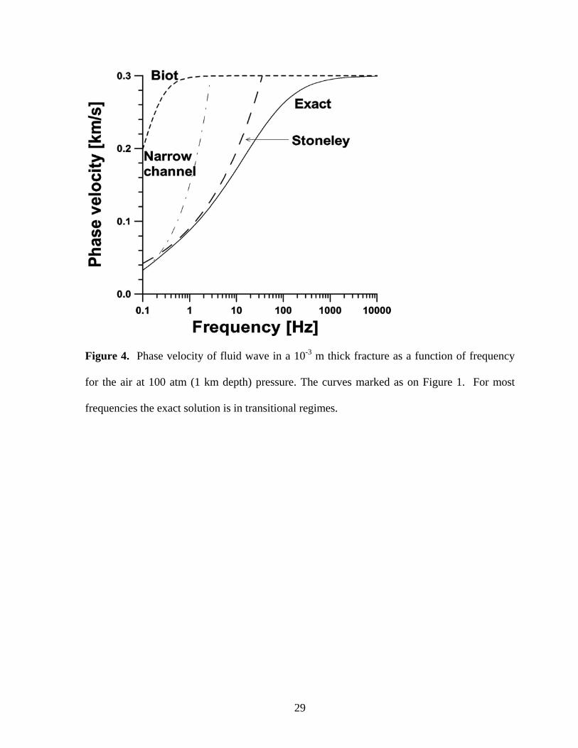
Figure 4. Phase velocity of fluid wave in a 10-3 m thick fracture as a function of frequency

for the air at 100 atm (1 km depth) pressure. The curves marked as on Figure 1. For most

frequencies the exact solution is in transitional regimes.

29

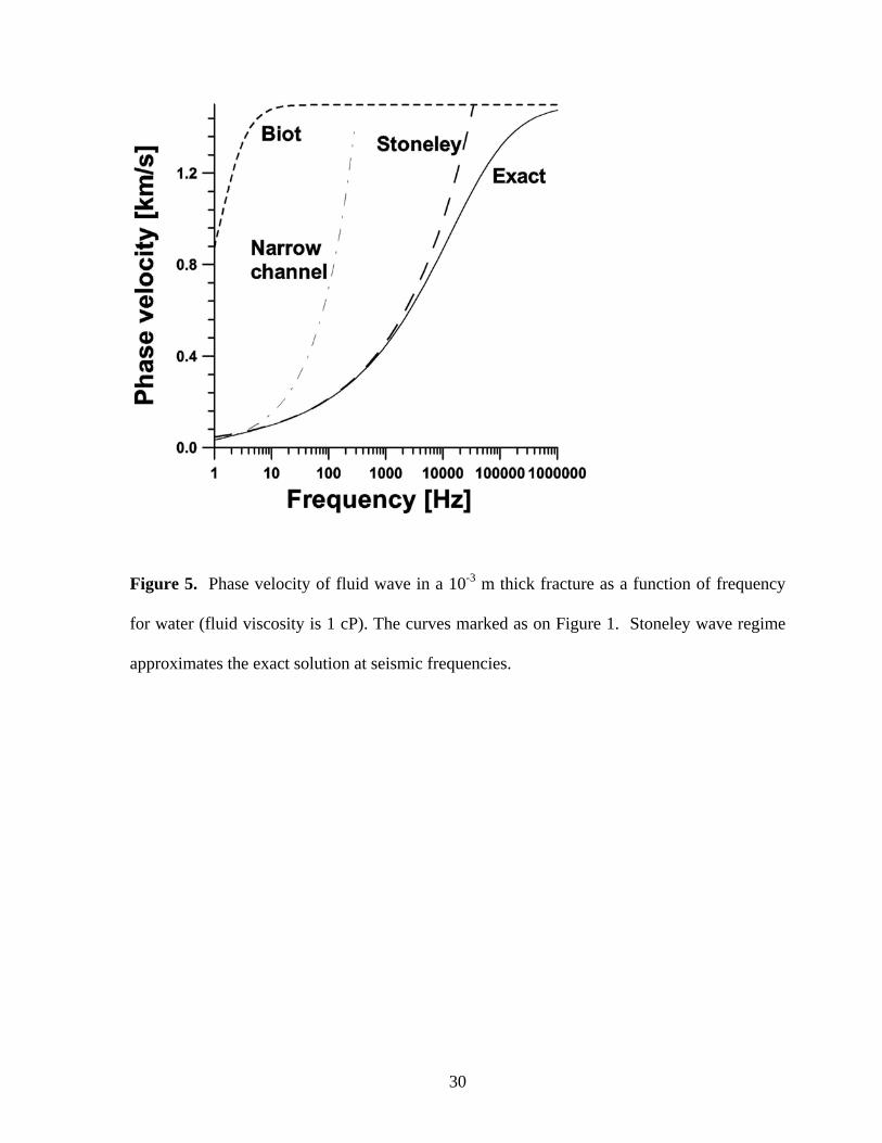
Figure 5. Phase velocity of fluid wave in a 10-3 m thick fracture as a function of frequency

for water (fluid viscosity is 1 cP). The curves marked as on Figure 1. Stoneley wave regime

approximates the exact solution at seismic frequencies.

30

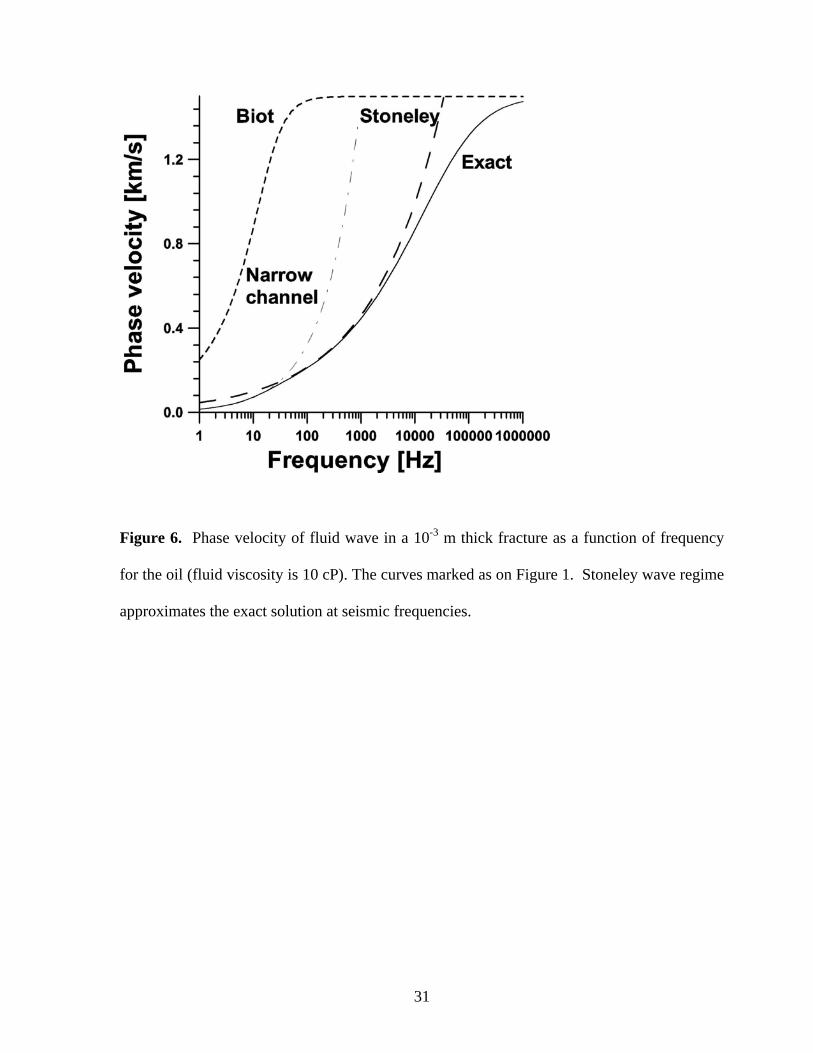
Figure 6. Phase velocity of fluid wave in a 10-3 m thick fracture as a function of frequency

for the oil (fluid viscosity is 10 cP). The curves marked as on Figure 1. Stoneley wave regime

approximates the exact solution at seismic frequencies.

31

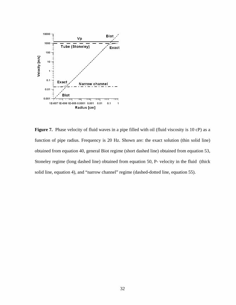
Figure 7. Phase velocity of fluid waves in a pipe filled with oil (fluid viscosity is 10 cP) as a

function of pipe radius. Frequency is 20 Hz. Shown are: the exact solution (thin solid line)

obtained from equation 40, general Biot regime (short dashed line) obtained from equation 53,

Stoneley regime (long dashed line) obtained from equation 50, P- velocity in the fluid (thick

solid line, equation 4), and “narrow channel” regime (dashed-dotted line, equation 55).

32

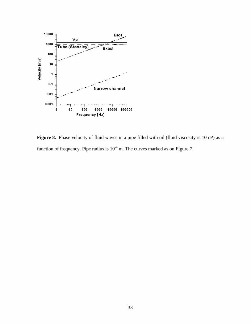
Figure 8. Phase velocity of fluid waves in a pipe filled with oil (fluid viscosity is 10 cP) as a

function of frequency. Pipe radius is 10-4 m. The curves marked as on Figure 7.

33

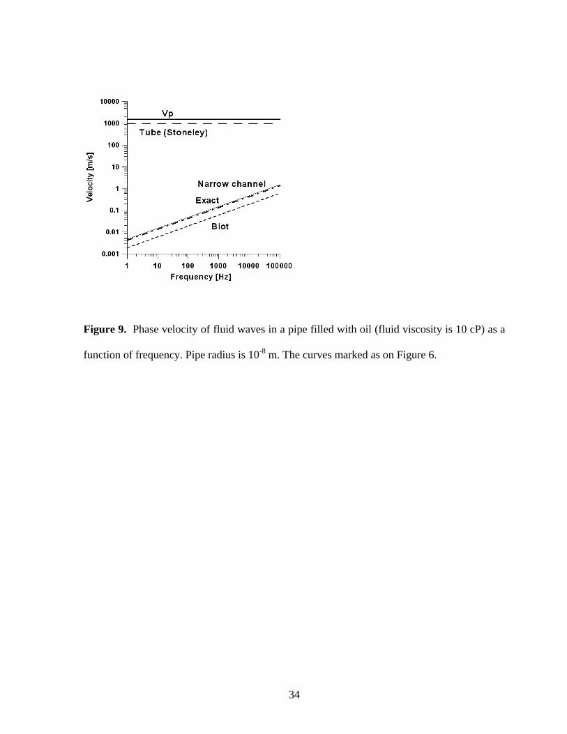
Figure 9. Phase velocity of fluid waves in a pipe filled with oil (fluid viscosity is 10 cP) as a

function of frequency. Pipe radius is 10-8 m. The curves marked as on Figure 6.

34

APPENDIX A

Cylindrical vector system

The cylindrical vector system used in this paper was introduced by Korneev and Johnson

(1993). Use of those vectors makes expressions for the Lamé equation especially simple since they

thoroughly imply a special symmetry of the problem. They allow formulation of wave propagation

problems in displacements, avoiding the potentials.

The cylindrical vector system has the form

30 eY mm Y , 1 2

1( )

2m m mY iY Y e e , 1 2

1(

2m m mY iY Y e )e , (A1)

where

( , ) exp ( )m m zY Y z i m h z , ,...2,1,0m , (A2)

and is the projection of the wavenumber onto the OZ-axis, zh 1i . Vectors are the

natural unit vectors of the cylindrical coordinate system ( ,

321 ,, eee

, )r z .

The cylindrical vectors of the system in (A1) are orthonormal at any point on a cylindrical

surface. In the space of vector functions 20),( f

defined on a circle

the vectors (A1) satisfy the following orthogonality relations ., .r const z const

1

1 1

2

0

( )m m mmd

1 Y Y , ,,0 (A3)

where kl is equal to 1, when lower indexes are the same, and equal zero otherwise.

The system A1 is complete in the sense of convergence in the mean for a Fourier series

expansion. This means that any vector function

( , , ) ( , ) exp( )zu u r z U r ih z

(A5)

can be represented in the form

0

( , , ) ( ) ( , )m mm

u r z f r z

Y

(A6)

The Lamé equation for a homogenous elastic medium is

35

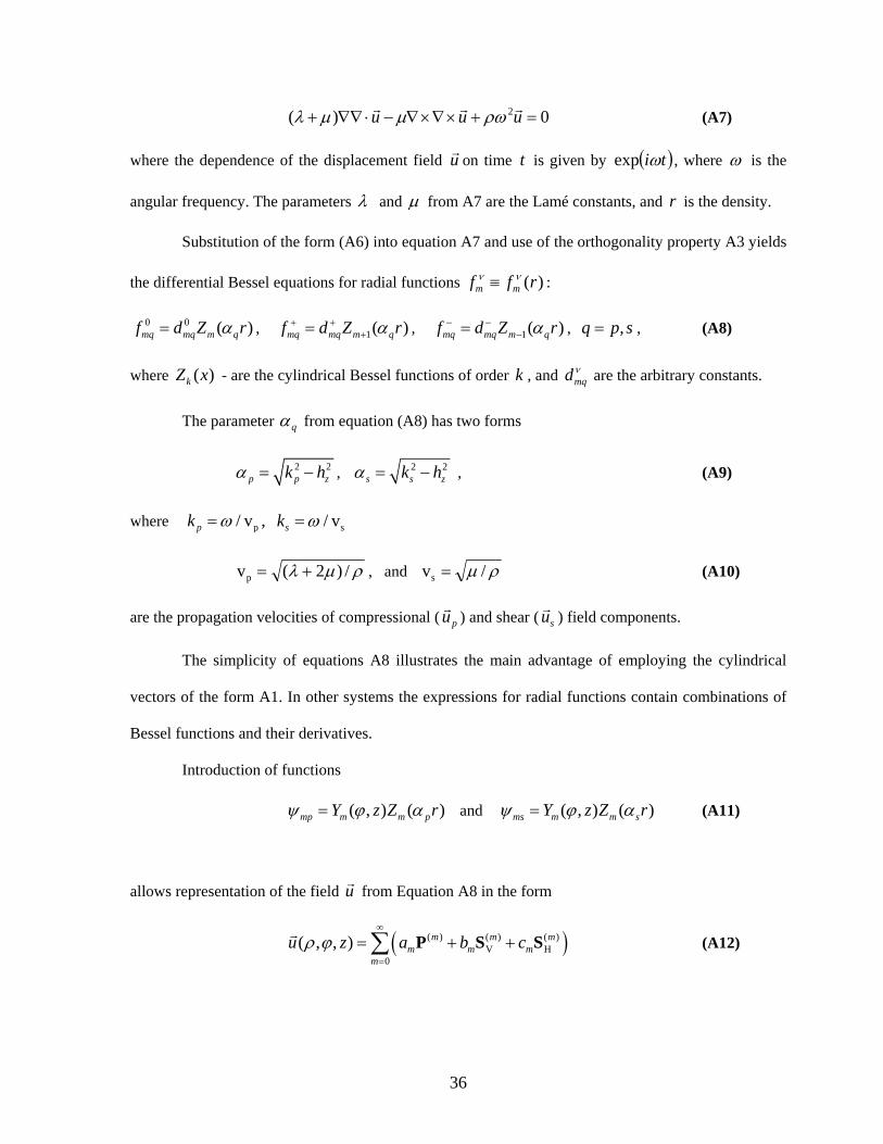
2( ) u u 0u

(A7)

where the dependence of the displacement field u

on time t is given by ti exp , where is the

angular frequency. The parameters and from A7 are the Lamé constants, and is the density. r

Substitution of the form (A6) into equation A7 and use of the orthogonality property A3 yields

the differential Bessel equations for radial functions ( )m mf f r :

0 0 (mq mq m q )f d Z r , 1(mq mq m q )f d Z r , 1( )mq mq m qf d Z r

, spq , , (A8)

where - are the cylindrical Bessel functions of order , and )(xZk k mqd are the arbitrary constants.

The parameter q from equation (A8) has two forms

2 2p pk h z , 2 2

s s zk h , (A9)

where p/ vpk , s/ vsk

/)2(vp , and /vs (A10)

are the propagation velocities of compressional ( pu

) and shear ( su

) field components.

The simplicity of equations A8 illustrates the main advantage of employing the cylindrical

vectors of the form A1. In other systems the expressions for radial functions contain combinations of

Bessel functions and their derivatives.

Introduction of functions

( , ) ( )mp m m pY z Z r and ( , ) ( )ms m m sY z Z r (A11)

allows representation of the field u from Equation A8 in the form

(A12) ( ) ( ) ( )V H

0

( , , ) m mm m m

m

u z a b c

P S S m

36

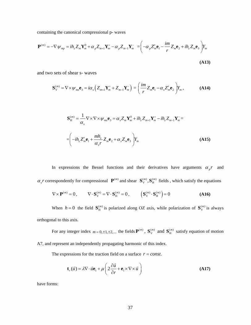
containing the canonical compressional p- waves

( ) 01 1

mmp z m m p m m p m mih Z Z Z

P Y Y Y = 1 2 3p m m z m m

imZ Z ih Z

r

e e e Y

1

(A13)

and two sets of shear s- waves

( )V 3 1m

ms s m m m mi Z Z S e Y Y = 1 2m s m

immZ Z Y

r

e e

, (A14)

( ) 0H 3 1

1mms s m m z m m z m m

s

Z ih Z ih Z 1

S e Y Y Y =

= 1 2z

z m m s m ms

mhih Z Z Z Y

r

e e e3 (A15)

In expressions the Bessel functions and their derivatives have arguments pr and

sr correspondently for compressional and shear fields , which satisfy the equations ( )mP ( ) ( )V H,m mS S

( ) 0m P , , ( ) ( )V H 0m m S S ( ) ( )

V H 0m m S S (A16)

When the field is polarized along OZ axis, while polarization of is always

orthogonal to this axis.

0h ( )HmS ( )

VmS

For any integer index the fields , and satisfy equation of motion

A7, and represent an independently propagating harmonic of this index.

0, 1, 2,...m ( )mP ( )

VmS ( )

HmS

The expressions for the traction field on a surface .r const

1 1( ) 2r

uu u

r

t e e u

(A17)

have forms:

37

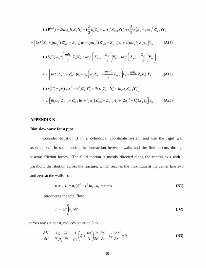
( ) 0 2 2 2 21 1( ) 2 ( ) ( )

2 2m

r p z m m p m p m m p m pi h Z k Z Z k Z Zm m

t P Y Y Y

e

(A18) 2 2 21 1 1 1 1 2 3( ( )) ( ) 2p m p m m p m m p z m mk Z Z Z i Z Z i h Z Y e e

( ) 0 2 2V 1( )

2 2m m mz

r m m s m m s m

Z ZmhZ i Z i Z

r 1 m

t S Y Y Y

= 21 1 1 1 1 2 3

1( ) z

s m m s s m m m

mhmi Z Z Z Z Z Y

r r

e e me

1

(A19)

( ) 2 2 0H 1( ) (2 )m

r s s m m z s m m z s m mk Z ih Z ih Z t S Y Y Y

= (A20) 2 21 1 1 1 1 2 3( ) ( ) (2 )z s m m z s m m s s m mih Z Z h Z Z k Z Y e e e

APPENDIX B Biot slow wave for a pipe

Consider equation 3 in a cylindrical coordinate system and use the rigid wall

assumption. In such model, the interaction between walls and the fluid occurs through

viscous friction forces. The fluid motion is mostly directed along the central axis with a

parabolic distribution across the fracture, which reaches the maximum at the center line z=0

and zero at the walls, so

2 21 0( )zu u R r u z z1 0 .u const, (B1)

Introducing the total flow

0

2R

zF u r dr (B2)

across any z = const, reduces equation 3 to

2 22

2 2 2 2

8 1 40

3 Pf f

F F F Fc

t R t z t z

2

(B3)

38

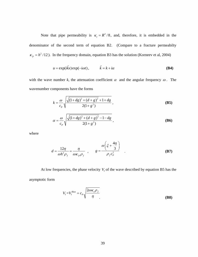
Note that pipe permeability is , and, therefore, it is embedded in the

denominator of the second term of equation B2. (Compare to a fracture permeabilty

). In the frequency domain, equation B3 has the solution (Korneev et al, 2004)

2 / 8c R

2 /12fr h

exp( )exp( )u ikx i t , k k i (B4)

with the wave number k, the attenuation coefficient and the angular frequency . The

wavenumber components have the forms

2 2

2

(1 ) ( ) 1

2(1 )P

dg d g dgk

c g

, (B5)

2 2

2

(1 ) ( ) 1

2(1 )P

dg d g dg

c g

, (B6)

where

, . (B7) 2

43

f P

gc

2

12

f fr f

dh

At low frequencies, the phase velocity of the wave described by equation B5 has the

asymptotic form

fV

. (B8)

Biotf f

2= c f

PV V c

39

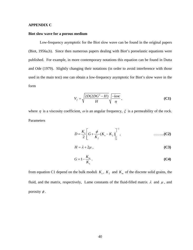
APPENDIX C Biot slow wave for a porous medium

Low-frequency asymptotic for the Biot slow wave can be found in the original papers

(Biot, 1956a,b). Since then numerous papers dealing with Biot’s poroelastic equations were

published. For example, in more contemporary notations this equation can be found in Dutta

and Ode (1979). Slightly changing their notations (in order to avoid interference with those

used in the main text) one can obtain a low-frequency asymptotic for Biot’s slow wave in the

form

22 (2 )f

D DG H iV

H

, (C1)

where is a viscosity coefficient, is an angular frequency, is a permeability of the rock.

Parameters

1

(2

ss f

f

KD G K K

K

)

, ……...(C2)

2H , (C3)

1 m

s

KG

K . (C4)

from equation C1 depend on the bulk moduli sK , fK and of the discrete solid grains, the

fluid, and the matrix, respectively, Lame constants of the fluid-filled matrix

mK

and , and

porosity .

40

DISCLAIMER This document was prepared as an account of work sponsored by the United States Government. While this document is believed to contain correct information, neither the United States Government nor any agency thereof, nor The Regents of the University of California, nor any of their employees, makes any warranty, express or implied, or assumes any legal responsibility for the accuracy, completeness, or usefulness of any information, apparatus, product, or process disclosed, or represents that its use would not infringe privately owned rights. Reference herein to any specific commercial product, process, or service by its trade name, trademark, manufacturer, or otherwise, does not necessarily constitute or imply its endorsement, recommendation, or favoring by the United States Government or any agency thereof, or The Regents of the University of California. The views and opinions of authors expressed herein do not necessarily state or reflect those of the United States Government or any agency thereof or The Regents of the University of California. Ernest Orlando Lawrence Berkeley National Laboratory is an equal opportunity employer.