Embed Size (px)
Citation preview
Low-Authority Controller Design via ConvexOptimization
To Appear in AIAA J. Guidance, Control, and Dynamics
Arash Hassibi∗ Jonathan How† Stephen Boyd‡
Information Systems Laboratory
Stanford UniversityStanford, CA 94305-9510
Email: [email protected] [email protected]
Telephone: (650) 723-9833 Fax: (650) 723-8473
May 20, 1999
∗Ph.D. candidate, Dept. of Electrical Engineering, Stanford University. Research supported byAir Force (under F49620-97-1-0459)
†Assistant Professor, Dept. of Aeronautics and Astronautics, Member AIAA, IEEE, AssociateMember ASME.
‡Professor, Dept. of Electrical Engineering, Stanford University. Research supported in partby AFOSR (under F49620-95-1-0318), NSF (under ECS-9222391 and EEC-9420565), and MURI(under F49620-95-1-0525).
Abstract
In this paper we address the problem of low-authority controller (LAC) design. The premiseis that the actuators have limited authority, and hence cannot significantly shift the eigen-values of the system. As a result, the closed-loop eigenvalues can be well approximatedanalytically using perturbation theory. These analytical approximations may suffice to pre-dict the behavior of the closed-loop system in practical cases, and will provide at least a verystrong rationale for the first step in the design iteration loop. We will show that LAC designcan be cast as convex optimization problems that can be solved efficiently in practice usinginterior-point methods. Also, we will show that by optimizing the `1 norm of the feedbackgains, we can arrive at sparse designs, i.e., designs in which only a small number of thecontrol gains are nonzero. Thus, in effect, we can also solve actuator/sensor placement orcontroller architecture design problems.
Keywords: Low-authority control, actuator/sensor placement, linear operator perturbationtheory, convex optimization, second-order cone programming, semi-definite programming,linear matrix inequality.
1 Introduction
The premise in low-authority control (LAC) is that the actuators have limited authority, and
hence cannot significantly shift the eigenvalues of the system [1, 2]. As a result, the closed-
loop eigenvalues can be well approximated analytically using perturbation theory. These
analytical approximations may suffice to predict the behavior of the closed-loop system in
practical cases, and will provide at least a very strong rationale for the first step in the design
iteration loop.
An important use of LAC is in lightly damped large structures with an infinite number
of elastic modes, where LAC is used to provide a small amount of damping in a wide range
of modes for maximum robustness. A high-authority controller (HAC) is then used around
the LAC to achieve high damping or mode-shape adjustment in a selected number of modes
to meet performance requirements.
In this paper we introduce a new method for low-authority controller design, based
on convex programming. We formulate the LAC design problem as a nonlinear convex
optimization problem, which can then be solved efficiently by interior-point methods. The
advantage of formulating the problem as convex is that very large order problems can be
solved (globally) in practice. Another advantage of this formulation is that it can handle
a very wide variety of specifications and objectives beyond standard eigenvalue-placement.
Typical design objectives for the LAC design include increased damping or decay rate for
the system response, and typical constraints include limitations on the controller gains and
actuator power. We show that by optimizing the `1 norm of the gains, we can arrive at sparse
designs, i.e., designs in which only a small number of the control gains are nonzero. Thus, in
effect, we can also solve actuator/sensor placement or controller architecture design problems.
Moreover, it is possible to address the robustness of the LAC, i.e., closed-loop performance
subject to uncertainties or variations in the plant model. Therefore, by combining all these,
for example, we can solve the problem of robust actuator/sensor placement and LAC design
in one step.
Although LAC design has been traditionally used for eigenvalue-placement, by using
powerful Lyapunov methods it is possible to extend LAC design to specifications beyond
eigenvalue-placement. These include bounds on output energy, quadratic costs on the state
and control input, induced L2 gain, etc.
The paper is organized as follows. The next section poses the problem statement, which is
followed by a section that presents typical applications of LAC. Section 4 is a brief overview of
convex programming, and in particular, linear, second-order cone, and semi-definite program-
1
ming. Section 5 discusses the first order perturbation formulas for the matrix eigenvalues,
and how the design problem can be posed within convex optimization framework. Section 6
discusses the sparsity of the solution, which is important for the control architecture stud-
ies. Section 7 addresses robust LAC design, i.e., a LAC design that guarantees performance
subject to uncertainties or variations in the plant model. Section 8 introduces an extension
to LAC design based on Lyapunov methods, and it is shown how additional performance
objectives (other than eigenvalue-placement) can be included in the formulation. Finally,
Sections 9 demonstrates the application of the methods on a few example problems.
2 Problem statement
We consider the linear time-invariant system
z = A(x)z, z(0) = z0, (1)
where z(t) ∈ Rn is the state, x ∈ Rq is a (design) parameter, and A(x) ∈ Rn×n is dif-
ferentiable at x = 0. The goal is to find x so that the system has sufficient damping, or
more generally, the eigenvalues of the system are in some desired region of the complex
plane. However, it is assumed that there is “limited authority” in designing x so that the
eigenvalues of system (1) are only slightly different from the eigenvalues of the unperturbed
system
z = A(0)z, z(0) = z0, (2)
i.e., system (1) with x = 0. Therefore, first order perturbation methods can be used to
predict the eigenvalue locations of system (1) from the eigenvalue locations of system (2).
We will refer to (1) and (2) as the closed-loop and open-loop systems respectively.
In many applications, it is desirable to achieve the required eigenvalue locations (or damp-
ing) when x has the minimum number of nonzero elements. In such cases, each nonzero xi
may correspond to a sensor, an actuator, a dissipating mechanism, or a structural com-
ponent, and therefore, reducing the number of nonzero xis simplifies the implementation.
Hence, we will also address the problem of minimizing the number of nonzero elements of x
such that the eigenvalues of system (1) are in some desired region of the complex plane.
In addition, we will consider robust LAC design, i.e., a LAC design with guaranteed
closed-loop system performance subject to uncertainties for variations in the system, as well
as LAC design for performance measures beyond eigenvalue-placement.
2
3 Applications of LAC
A key control design methodology for flexible systems with many elastic modes follows the
two-level architecture presented in [1, 3, 2, 4]. This architecture consists of a wide-band,
low-authority control (LAC) and a narrow-band, high-authority control (HAC). Within this
framework, the HAC is designed based on a (low-order) finite-dimensional model of the
structure, and provides high damping or mode-shape adjustment in a selected number of
modes to meet performance requirements. However, due to spillover, the HAC can destabilize
modes not included in the design model, which are usually at high frequency and poorly
known. LAC, on the other hand, introduces low damping in a wide range of modes for
maximum robustness. LAC is, therefore, necessary to reduce the destabilization problems
created by HAC. HAC, for example, could be a linear-quadratic-Gaussian (LQG) controller
using a collection of sensors and actuators. LAC, however, is usually implemented using
(active or passive) high-energy-dissipating mechanisms [5].
High-energy-dissipating mechanisms are usually incorporated into the structure by using
layers of viscoelastic shear damping material. In the simplest case, the force-extension char-
acteristic of viscoelastic material can be modeled as a combination of a linear spring and
a dash-pot, where the stiffness and damping is related to the geometry of the dissipating
mechanism and the amount of viscoelastic material used. Hence, in the framework (1) the
parameter x represents, for example, the amount of viscoelastic material at various locations
of the structure. A zero xi would mean that the dissipating mechanism at the corresponding
location is not needed, so in many cases it is desirable to find an x with as many zero com-
ponents as possible (subject to the control design specifications) to obtain a simple design.
Linear state-feedback LAC design is another example that can be easily cast in the
framework (1). We may require the state-feedback gain to satisfy certain constraints (e.g.,
on the size of its components or its sparsity pattern), or find a state-feedback gain that is
sparse (so that a small number of sensors/actuators are needed and the controller has a
simple topology). This state-feedback approach is particularly useful for the (collocated)
rate-feedback design often used for LAC. Specifically, suppose that
z = Az + Bu, u = Kz,
where A ∈ Rn×n and B ∈ Rn×m are given and K ∈ Rm×n should be found to achieve, say,
sufficient damping. The closed-loop system becomes z = (A + BK)z and by taking x to
be the elements of K this problem falls into the framework (1). A sparse K represents a
simple controller topology since sparsity implies that we only need to connect each sensor to
3
a few actuators. Moreover, a zero row (column) in K means that the corresponding actuator
(sensor) is not required.
More generally, we can also consider dynamic LAC design for the open-loop system
z = Az + Bu, y = Cz,
where the controller is parameterized by its state-space system matrices Ac, Bc, Cc, Dc, and
is given by
zc = Aczc + Bcy, u = Cczc + Dcy.
The closed-loop system can be written as z
zc
=
A + BDcC BCc
BcC Ac
z
zc
,
which is in the form ˙z = A(x)z where z = [zT zTc ]T , and x represents the elements of the
controller system matrices Ac, Bc, Cc, and Dc. By requiring sparsity for Bc, Cc, and Dc we
can find designs that require a small number of actuators and sensors.
Another problem that can be formulated in the LAC framework is that of structural
design and optimization [6]. In such a case, x can include various parameters such as beam
widths, beam lengths, masses, dampers, etc. The best design, for example, is a structure
that supports specified loads at fixed points, achieves acceptable dynamic behavior such as
sufficient damping, and at the same time, has the simplest topology or minimum weight.
4 Linear, second-order cone, and semi-definite program-
ming
In this section we briefly introduce linear, second-order cone, and semi-definite programs
which are families of convex optimization problems that can be efficiently solved (globally)
using interior-point methods [7, 8]. In later sections, we will see how LAC design can be cast
in terms of linear, second-order cone, or semi-definite programs and hence solved efficiently
in practice.
A linear program (LP) is an optimization problem with linear objective and linear equality
and inequality constraints:
minimize cT x
subject to fTi x ≤ gi, i = 1, . . . , J,
Ax = b,
(3)
4
where the vector x is the optimization variable and c, fi, gi, A, and b are problem parameters.
Linear programming has been used in a wide variety of fields. In control, for example,
Zadeh and Whalen observed in 1962 that certain minimum-time and minimum-fuel optimal
control problems could be (numerically) solved by linear programming [9]. In the late 70s,
Richalet [10] developed model predictive control (also known as dynamic matrix control or
receding horizon control), in which linear or quadratic programs are used to solve an optimal
control problem at each time step. Model predictive control is now widely used in the process
control industry. Several high quality, efficient implementations of interior-point LP solvers
are available (see, e.g., [11, 12, 13]).
A semi-definite program (SDP), is an optimization problem which has the form
minimize cT x
subject to x1F1 + · · ·+ xmFm � G,
Ax = b
(4)
where Fi and G are symmetric p×p matrices, and the inequality � denotes matrix inequality,
i.e., X � Y means Y − X is positive semi-definite. The constraint x1F1 + · · · + xmFm � G
is called a linear matrix inequality (LMI). While SDPs look complicated and would ap-
pear difficult to solve, new interior-point methods can solve them with great efficiency (see,
e.g., [8, 14]) and several SDP codes are now widely available [15, 16, 17, 18, 19, 20]. The
ability to numerically solve SDPs with great efficiency is being applied in several fields, e.g.,
combinatorial optimization and control [21]. SDP is currently a highly active research area.
A second-order cone program (SOCP) has the form
minimize cT x
subject to ‖Fix + gi‖ ≤ cTi x + di, i = 1, . . . , L,
Ax = b,
(5)
where ‖ · ‖ denotes the Euclidean norm, i.e., ‖z‖ =√
zT z. SOCPs include linear and
quadratic programming as special cases, but can also be used to solve a variety of nonlinear,
nondifferentiable problems; see, e.g., [22]. Moreover, efficient interior-point software for
SOCP is now available [23, 24].
As a final note, it should be mentioned that among the three different class of optimization
problems mentioned, SDP is the most general, and includes LP and SOCP as special cases.
5
5 Eigenvalue-placement LAC design using linear and
second-order cone programming
In this section we show that analytic first order perturbation formulas for eigenvalues of
a matrix can be used to design low-authority controllers using linear or second-order cone
programming for eigenvalue-placement specifications. As mentioned in §4, linear and second-
order cone programs can be solved very efficiently, and therefore, this gives an efficient
method for LAC design.
5.1 First order perturbation formulas for eigenvalues of a matrix
A typical problem of the perturbation theory for linear operators is to investigate how the
eigenvalues of a linear operator A ∈ Rn×n change when A is subjected to small perturbation.
For example, consider the family of operators A(x) ∈ Rn×n where A(0) = A and x ∈ Rq is
a parameter supposed to be small. A question arises whether the eigenvalues of A(x) can
be expressed as a power series in x, i.e., whether they are holomorphic functions of x in the
neighborhood of x = 0.
In [25] it is shown that if A(x) is k-times continuously differentiable in x on a simply-
connected domain D ⊂ Rq, and the number of eigenvalues λi(x) of A(x) corresponding to a
Jordan block of size 1 is constant for x ∈ D, then each λi(x) is also k-times continuously dif-
ferentiable. Therefore, the change of these eigenvalues will be of the same order of magnitude
as the perturbation for small ‖x‖. Specifically we have
λi(x) = λi +q∑
k=1
(w∗
i Akui
w∗i ui
)xk + o(‖x‖), (6)
where ui ∈ Cn, wi ∈ Cn are the left and right eigenvectors of A(0) corresponding to the
eigenvalue λi ∈ C, and Ak = ∂A(0)/∂xk for k = 1, . . . , q. Equation (6) gives the first order
expansion formula for the eigenvalues of the perturbed matrix A(x).
Remark. If λi is a repeated eigenvalue of A(0) corresponding to a Jordan block ofsize pi > 1, λi(x) is no longer given as in (6). In this case λi(x) is given by a Puiseuxseries such as
λi(x) = λi +q∑
k=1
αikx1/pi
k +q∑
k=1
q∑j=1
βikjx1/pi
k x1/pi
j + · · · .
In other words, the change in the eigenvalue is not of the same order of magnitude asthe perturbation of the matrix for small ‖x‖.
6
5.2 LAC eigenvalue-placement design using linear or second-order
cone programming
Let Di ⊂ C be the desired region for λi(x), the ith eigenvalue of A(x). We assume that Di
is either polyhedral (an intersection of Ji half-planes) given by
Di = { s ∈ C | aij Re(s) + bij Im(s) ≤ cij , j = 1, . . . , Ji }, (7)
where aij ∈ R, bij ∈ R, cij ∈ R, or an intersection of second-order cones given by
Di = { s ∈ C |∥∥∥∥∥∥Fi
Re(s)
Im(s)
+ gi
∥∥∥∥∥∥ ≤ cTi
Re(s)
Im(s)
+ di }, (8)
where Fi ∈ R2×2, gi ∈ R2, ci ∈ R2, di ∈ R, in which Re(s) and Im(s) are the real and
imaginary parts of s ∈ C respectively (examples of these regions will follow shortly).
Under the low-authority control assumption, we can drop the o(‖x‖) term in equation (6)
without significant error, and λi(x) becomes approximately linear in the design variable x.
From (6)
Re (λi(x)) ≈ Re (λi) +∑q
k=1 Re(
w∗i Akui
w∗i ui
)xk,
Im (λi(x)) ≈ Im (λi) +∑q
k=1 Im(
w∗i Akui
w∗i ui
)xk,
and therefore to first order λi(x) ∈ Di as defined in (7) if and only if for j = 1, . . . , Ji
aij
(Re (λi) +
q∑k=1
Re
(w∗
i Akui
w∗i ui
)xk
)+ bij
(Im (λi) +
q∑k=1
Im
(w∗
i Akui
w∗i ui
)xk
)≤ cij,
or equivalently
q∑k=1
(aij Re
(w∗
i Akui
w∗i ui
)+ bij Im
(w∗
i Akui
w∗i ui
))xk ≤ cij − aij Re (λi) − bij Im (λi) , (9)
which is a linear inequality constraint in the variable x ∈ Rq.
Similarly, if we require that λi(x) fall inside the second-order conic region Di as in (8),
to first order we must have∥∥∥∥∥∥Fi
Re(
w∗i A1ui
w∗i ui
)· · · Re
(w∗
i Aqui
w∗i ui
)Im
(w∗
i A1ui
w∗i ui
)· · · Im
(w∗
i Aqui
w∗i ui
) x + Fi
Re(λi)
Im(λi)
+ gi
∥∥∥∥∥∥ ≤
cTi
Re(
w∗i A1ui
w∗i ui
)· · · Re
(w∗
i Aqui
w∗i ui
)Im
(w∗
i A1ui
w∗i ui
)· · · Im
(w∗
i Aqui
w∗i ui
) x + cT
i
Re(λi)
Im(λi)
+ di,
(10)
7
which is a second-order cone constraint in x ∈ Rq.
Suitable objectives are usually ones that require x to be in some sense “small”. These
include different norms on x such as ‖x‖1, ‖x‖2, and ‖x‖∞. For example, minimizing ‖x‖1
or ‖x‖∞ subject to (9) leads to LPs (after adding slack variables), while minimizing any of
these norms subject to (9) or (10) leads to SOCPs. Therefore, the LAC eigenvalue-placement
problem can be easily cast as an LP or SOCP that can be solved very efficiently.
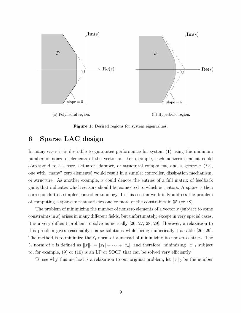
Consider a typical example which is to place the eigenvalues of system (1) in the shaded
region of Figure 1(a) (damping of at least 0.1, damping ratio of at least 0.2), and the objective
is to minimize the sum of the entries of x. In this case, for i = 1, . . . , n
Re (λi(x)) ≤ −0.1, Im (λi(x)) ± 5Re (λi(x)) ≤ 0.
Therefore, the optimization problem becomes (to first order)
minimize x1 + x2 + · · ·+ xq
subject to∑q
k=1 Re(
w∗i Akui
w∗i ui
)xk ≤ −0.1 −Re (λi) ,∑q
k=1
(Im
(w∗
i Akui
w∗i ui
)± 5Re
(w∗
i Akui
w∗i ui
))xk ≤ − Im (λi) ∓ 5Re (λi) ,
i = 1, . . . , n,
which is an LP in x. (Of course because of conjugate symmetry of the eigenvalues not all of
the linear inequality constraints need to be imposed).
As another example, if the eigenvalues are to be placed in the hyperbolic region D of
Figure 1(b), i.e., {s | (√
Im(s)2 ≤ −5Re(s)− 0.5}, and the objective is the same as before,
according to (10) we get the optimization problem
minimize x1 + x2 + · · ·+ xq
subject to
∥∥∥∥∥∥ Im(λi)
0
+
Im(
w∗i A1ui
w∗i ui
)· · · Im
(w∗
i Aqui
w∗i ui
)0 · · · 0
x
∥∥∥∥∥∥ ≤
−5[
Re(
w∗i A1ui
w∗i ui
)· · · Re
(w∗
i Aqui
w∗i ui
) ]x − 5Re(λi) − 0.5, i = 1, . . . , n,
which is an SOCP in x.
Note that we can also mix the linear inequality and second-order cone constraints (9)
and (10) with other constraints on x. For example, we may require that 0 ≤ xi ≤ xi,max
(xi,max is given) corresponding to, say, physical limitations on the values of xi. As long as
these conditions are linear equality, linear inequality, or second-order cone constraints in x,
they can be easily dealt within an efficient optimization program.
8
Re(s)
Im(s)
−0.1
slope = 5
D
(a) Polyhedral region.
Re(s)
Im(s)
−0.1
slope = 5
D
(b) Hyperbolic region.
Figure 1: Desired regions for system eigenvalues.
6 Sparse LAC design
In many cases it is desirable to guarantee performance for system (1) using the minimum
number of nonzero elements of the vector x. For example, each nonzero element could
correspond to a sensor, actuator, damper, or structural component, and a sparse x (i.e.,
one with “many” zero elements) would result in a simpler controller, dissipation mechanism,
or structure. As another example, x could denote the entries of a full matrix of feedback
gains that indicates which sensors should be connected to which actuators. A sparse x then
corresponds to a simpler controller topology. In this section we briefly address the problem
of computing a sparse x that satisfies one or more of the constraints in §5 (or §8).
The problem of minimizing the number of nonzero elements of a vector x (subject to some
constraints in x) arises in many different fields, but unfortunately, except in very special cases,
it is a very difficult problem to solve numerically [26, 27, 28, 29]. However, a relaxation to
this problem gives reasonably sparse solutions while being numerically tractable [26, 29].
The method is to minimize the `1 norm of x instead of minimizing its nonzero entries. The
`1 norm of x is defined as ‖x‖1 = |x1| + · · · + |xq|, and therefore, minimizing ‖x‖1 subject
to, for example, (9) or (10) is an LP or SOCP that can be solved very efficiently.
To see why this method is a relaxation to our original problem, let ‖x‖0 be the number
9
of nonzero elements of x. Now consider the following optimization problem:
minimize ‖x‖0
subject to x ∈ C‖x‖∞ ≤ 1,
(11)
where C is some compact (convex) subset of Rn. (Note that by scaling variables, without
loss of generality, we can assume that ‖x‖∞ ≤ 1.) The optimization problem (11) can be
cast as the mixed optimization problem
minimize z1 + z2 · · · + zq
subject to x ∈ C|xi| ≤ zi
zi ∈ {0, 1}, i = 1, . . . , q.
Now if we relax the Boolean constraint zi ∈ {0, 1} by 0 ≤ zi ≤ 1 we get the optimization
problem
minimize z1 + z2 · · ·+ zq
subject to x ∈ C|xi| ≤ zi
0 ≤ zi ≤ 1, i = 1, . . . , q.
which is the same asminimize ‖x‖1
subject to x ∈ C‖x‖∞ ≤ 1.
(12)
Therefore, we have just shown that (12) is a natural relaxation to (11). (When we do not
have the constraint ‖x‖∞ ≤ 1, the natural relaxation will involve a weighted `1 norm.)
The `1 norm relaxation method usually tends to give acceptable sparse solutions. How-
ever, if we insist on finding the x with the least number of nonzero elements, we need to
enumerate all possible sparsity patterns of x and check them for feasibility (i.e., if there
exists an x with the given sparsity pattern that satisfy the constraints). Among all feasible
sparsity patterns of x, the one with the least number of nonzero elements minimizes ‖x‖0.
Since x has q components and each component is either zero or nonzero, the total number
of sparsity patterns of x is 2q. Therefore, in principle, by solving at most 2q feasibility
problems it is possible to find an x minimizing ‖x‖0. However, 2q could be very large for
even relatively small values of q, and as a result, finding the optimum x could be cumbersome.
Good heuristics on to how and in what order to check the different sparsity patterns of x
usually greatly reduce the necessary number of feasibility problems we need to solve. For
10
example, one heuristic is to use the solution to the `1 relaxation problem as a basis to decide
what sparsity patterns should be checked first. The idea is simply that it is “more probable”
for the ith component of the optimum solution to be nonzero if the ith component of the
solution to the relaxed problem is “large”.
7 Robust LAC design
In this section we address the problem of robust LAC design, i.e., a LAC design with
guaranteed (closed-loop) system performance subject to uncertainties or variations in the
system model. We show that it is possible to solve the robust LAC design problem using LP
and SOCP. Therefore, by combining the methods of this section and that of §6, we can handle
low-authority controller design, actuator/sensor placement, and robustness at the same time.
Robust actuator/sensor placement and robust controller design are usually performed in
two separate stages (and hence non-optimally) because it is numerically intractable to do
otherwise (see, e.g., [30] for a thorough overview of robust actuator and damper placement
for structural control). It is yet another numerical advantage of LAC design that it is possible
to handle both of these problems at one step very efficiently.
We will consider two different approaches for modeling the system uncertainty and will
show how to design a robust LAC in each case. The first approach is to consider a parametric
uncertainty, and the second approach is to model the uncertainty by a finite number of
possible system models. The uncertainty is assumed to be time-invariant in both cases.
7.1 Robust LAC design for systems subject to “small” parametric
uncertainties
As a generalization to the setup of §1, we assume that the dynamics of the (closed-loop)
system can be described as
z = A(x, δ)z (13)
where x ∈ Rq is the design parameter (as before), and δ ∈ Rr represents the model uncer-
tainty satisfying
−δi,max ≤ δi ≤ δi,max (14)
for i = 1, . . . , r in which δi,max is given. We assume that the low-authority assumption holds
and δ is “small” so that the eigenvalues of A(x, δ) can be well-approximated using (first
order) perturbation formulas. The goal is to find x such that for all possible values of δ,
the eigenvalues of (13) are in some desired region of the complex plane. Let Di ⊂ C be the
11
desired region for λi(x, δ), the ith eigenvalue of A(x, δ). We assume that Di is polyhedral as
in (7).
Using the Farkas Lemma (see, e.g., [6]) it can be shown that (to first order) λi(x, δ) ∈ Di
for all δ satisfying (14) if and only if there exists τ (1), τ (2) ∈ Rr such that
τ(1)l ≥ 0, τ
(2)l ≥ 0, τ
(1)l − τ
(2)l = aij Re
(w∗
i Alui
w∗i ui
)+ bij Im
(w∗
i Alui
w∗i ui
),
q∑k=1
(aij Re
(w∗
i Akui
w∗i ui
)+ bij Im
(w∗
i Akui
w∗i ui
))xk+
r∑l=1
(τ
(1)l + τ
(2)l
)δl,max ≤ cij − aij Re (λi) − bij Im (λi) ,
(15)
for l = 1, . . . , r and j = 1, . . . , Ji, which is a set of linear equality and inequality constraints
in x, τ (1), and τ (2). Hence, by minimizing ‖x‖1 subject to (15) for example, it is possible to
design robust and sparse LACs for eigenvalue-placement specifications subject to bounded
parametric uncertainties in the system model by solving LPs.
Note that using similar methods, it is possible to cast robust LAC design as an LP or
SOCP for cases in which Di is described as in (8), and/or δ is bound to lie in an ellipsoid.
Ellipsoidal (confidence) regions for δ may come from a statistical study of the uncertainties
in the system. For example, suppose that it is known that the uncertainty δ lies in the
ellipsoid { δ | ‖Fδ + g‖ ≤ 1 } where F ∈ Rr×r (full rank) and g ∈ Rr are known. It is easy
to verify that, to first order, the ith eigenvalue of (13) lies in Di as defined in (7) if and only
if
q∑k=1
(aij Re
(w∗
i Akui
w∗i ui
)+ bij Im
(w∗
i Akui
w∗i ui
))xk ≤
cij − aij Re (λi) − bij Im (λi) + ‖F−Tdij‖ + dTijF
−1g,
for j = 1, . . . , Ji where
dij = aij
[Re
(w∗
i A1ui
w∗i ui
)· · · Re
(w∗
i Arui
w∗i ui
) ]T+ bij
[Im
(w∗
i A1ui
w∗i ui
)· · · Im
(w∗
i Arui
w∗i ui
) ]T.
Again, these are a set of linear inequalities in x and can therefore be handled by solving LPs.
7.2 Robust LAC design for systems with multiple models
Here we consider a multiple model approach to robust LAC design. This approach relies
on the fact that it is possible to adequately model uncertainty or plant variation by a finite
number of system models
z = A(l)(x)z, l = 1, . . . , ν. (16)
12
For robust LAC design in this framework, the goal is to find x such that the eigenvalues of
each of the system models (16) are in some desired region of the complex plane. This can
be easily done by requiring the eigenvalue-placement specifications to hold for each of the
models.
For example, if the desired region Di of the ith eigenvalue is given as in (7), then using
perturbation formulas from §5.1 we require that
q∑k=1
aij Re
w(l)∗i A
(l)k u
(l)i
w(l)∗i u
(l)i
+ bij Im
w(l)∗i A
(l)k u
(l)i
w(l)∗i u
(l)i
xk ≤ cij − aij Re(λ
(l)i
)− bij Im
(λ
(l)i
),
(17)
for l = 1, . . . , ν, where λ(l)i , u
(l)i , and w
(l)i are the ith eigenvalue, right eigenvector, and
left eigenvector of A(l)(0) respectively. Therefore, in the robust case, eigenvalue-placement
specifications can still be described as LPs that are just ν times larger. Hence, robust LAC
design using a multiple model approach can be easily handled as before.
8 Extension: LAC design based on Lyapunov theory
In this section we show how Lyapunov theory can be used to design low-authority con-
trollers. Lyapunov methods are very powerful and enable us to formulate design objectives
beyond eigenvalue-placement specifications in terms of SDPs, which can then be solved very
efficiently (cf. §4). These design objectives can be combined to get, for example, a desired
eigenvalue location for the system while providing a bound on output energy, L2 gain, etc.
By combining the results of §6 and §7 with those presented here it is possible to perform
robust actuator/sensor placement or controller structure design that are optimum to first
order for a variety of control objectives. This would be very useful, for example, for HAC
structure design as well, since it will provide a rationale as to where the actuators/sensors
should be placed.
The method of LAC design using Lyapunov theory can be summarized as follows. Sup-
pose that the Lyapunov function V (z) = zT Pz, P � 0 proves some level of performance for
some property of the unperturbed or open-loop system (2). Then, under the low-authority
assumption, it is reasonable to assume that the Lyapunov function V (z) = zT (P + δP )z,
P + δP � 0 with δP “small” is a Lyapunov function candidate for the same property of
the closed-loop system (1). Therefore, as a first order approximation, we can neglect sec-
ond order (cross) terms such as xiδP in the (bilinear) matrix inequality conditions that are
equivalent to V being a Lyapunov function proving (a better) level of performance for the
closed-loop system. Hence, the matrix inequalities become jointly linear in x and δP , and
13
therefore, can be easily handled by solving SDPs.
In this section we illustrate this method for two different design specifications, but it
should be noted that the method is quite powerful, and can also be applied to handle many
other design specifications.
8.1 Bound on output energy
Consider the (closed-loop) linear dynamical system with output
z = A(x)z, y = C(x)z, z(0) = z0. (18)
The goal is to design x to “moderately” reduce the output energy∫∞0 yTy dt of the closed-
loop system (18) from that of the unperturbed or open-loop system (i.e., system (18) with
x = 0).
The output energy of the open-loop system is bounded by z(0)T Pz(0) for any P � 0
satisfying (see, e.g., [21])
A(0)TP + PA(0) + C(0)T C(0) � 0. (19)
(If the inequality in this equation is replaced by equality, z(0)T Pz(0) gives the exact output
energy). The output energy of the closed-loop system (18) is bounded by z(0)T (P + δP )z(0)
if there exists δP such that P + δP � 0 and
A(x)T (P + δP ) + (P + δP )A(x) + C(x)T C(x) � 0. (20)
Under the low-authority assumption it is reasonable to assume that δP and xi are “small”
and their product is to first order negligible. Hence, by expanding A(x) and C(x) in (20)
to their first order (Taylor) approximation, and neglecting the second order terms such as
xiδP we get
A(0)T P + PA(0) + C(0)TC(0) + A(0)T δP + δPA(0)+∑qk=1 xk
(AT
k P + PAk + C(0)T Ck + CTk C(0)
)� 0,
(21)
where Ak∆= ∂A(0)/∂xk, and Ck
∆= ∂C(0)/∂xk. (21) is an LMI in the variables δP ∈
Rn×n and x ∈ Rq although we will not write out the LMI explicitly in the standard form
x1F1 + · · · + xmFm � G of §4 (leaving LMIs in condensed form, in addition to saving
notation, may lead to more efficient computation). By adding the constraint P + δP � 0
(and constraining ‖δP‖ ≤ 0.2‖P‖I for example to ensure that the first order approximations
14
are accurate), a first order condition for an output energy of z(0)T (P +δP )z(0) for the closed-
loop system becomes
P + δP � 0,
0.2P δP
δP 0.2P
� 0,
A(0)T P + PA(0) + C(0)TC(0) + A(0)T δP + δPA(0)+∑qk=1 xk
(AT
k P + PAk + C(0)T Ck + CTk C(0)
)� 0,
(22)
where P is any positive definite matrix satisfying (19). (In this case it seems reasonable to
pick P as the unique solution to the Lyapunov equation A(0)TP +PA(0)+C(0)TC(0) = 0.)
By adding (linear) constraints such as z(0)T (P + δP )z(0) ≤ ε, Tr(P + δP ) ≤ η, etc., that
require the output energy to be smaller than some prescribed level, and by minimizing for
example ‖x‖1, LAC design for output energy specifications can be solved using SDP.
8.2 L2 gain
Consider the (closed-loop) linear dynamical system with input and output
z = A(x)z + B(x)w, y = C(x)z + D(x)w. (23)
Suppose that the induced L2 gain from input w to output y of the open-loop system, i.e.,
system (23) with x = 0, is less than γ so that [21] A(0)T P + PA(0) + C(0)T C(0) PB(0) + C(0)TD(0)
B(0)T P + D(0)TC(0) −γ2I + D(0)T D(0)
� 0. (24)
Then using a similar reasoning to §8.1, to first order, the induced L2 gain from input w to
output y of the closed-loop system is less than γ2 + δ(γ2) if
P + δP � 0,
0.2P δP
δP 0.2P
� 0,
A(0)T P + PA(0)+
C(0)T C(0) + A(0)T δP + δPA(0)+∑qk=1 xk
(AT
k P + PAk
)+∑q
k=1 xk
(C(0)T Ck + CT
k C(0))
(P + δP )B(0) + C(0)T D(0)+∑q
k=1 xk(PBTk + CT
k D(0) + C(0)T Dk)
B(0)T (P + δP ) + D(0)T C(0)+∑q
k=1 xk(BkP + D(0)TCk + DTk C(0))
−(γ2 + δ(γ2))I + D(0)T D(0)+∑qk=1 xk(D
Tk D(0) + D(0)Dk)
� 0,
(25)
where Ak∆= ∂A(0)/∂xk , Bk
∆= ∂B(0)/∂xk , Ck
∆= ∂C(0)/∂xk, and Dk
∆= ∂D(0)/∂xk. (25) is
an LMI in the variables δP = δP T , x, and δ(γ2).
15
Note that the method of this section works for any P that proves some level of perfor-
mance for the open-loop system (e.g., any P that satisfies (19) or (24)). This observation
highlights a potential weakness of this method because it is not clear which P should be
used in for example (21) or (25). However, we conjecture that it does not make much dif-
ference which P is chosen because the perturbations are assumed to be small and the P can
be adjusted using the free variable δP . Our experience indicates that the P with smallest
condition number, or the one that minimizes log det P−1, seems to work well in practice.
As a final remark, it should be noted that the different LAC design constraints in previous
sections can be mixed freely. Since these constraints were either linear inequalities, second-
order cone constraints, or LMIs, a semi-definite program solver (e.g., [17]) can be used to
compute the design parameter x very efficiently in practice.
For example, x can be a vector of feedback gains of different colocated sensor/actuator
pairs, and for the closed-loop system we may require a certain minimum amount of damping
and damping ratio in the eigenvalues (cf. §5.2), and a bound on the level of induced L2 norm
from an input to an output (cf. §8.2), while the ith feedback gain is absolutely bounded by
ximax (−xi,max ≤ xi ≤ xi,max). By minimizing say ‖x‖1 subject to these design specifications
we will (hopefully) obtain a sparse x and therefore many of the sensor/actuator pairs will
not be needed (cf. §6).
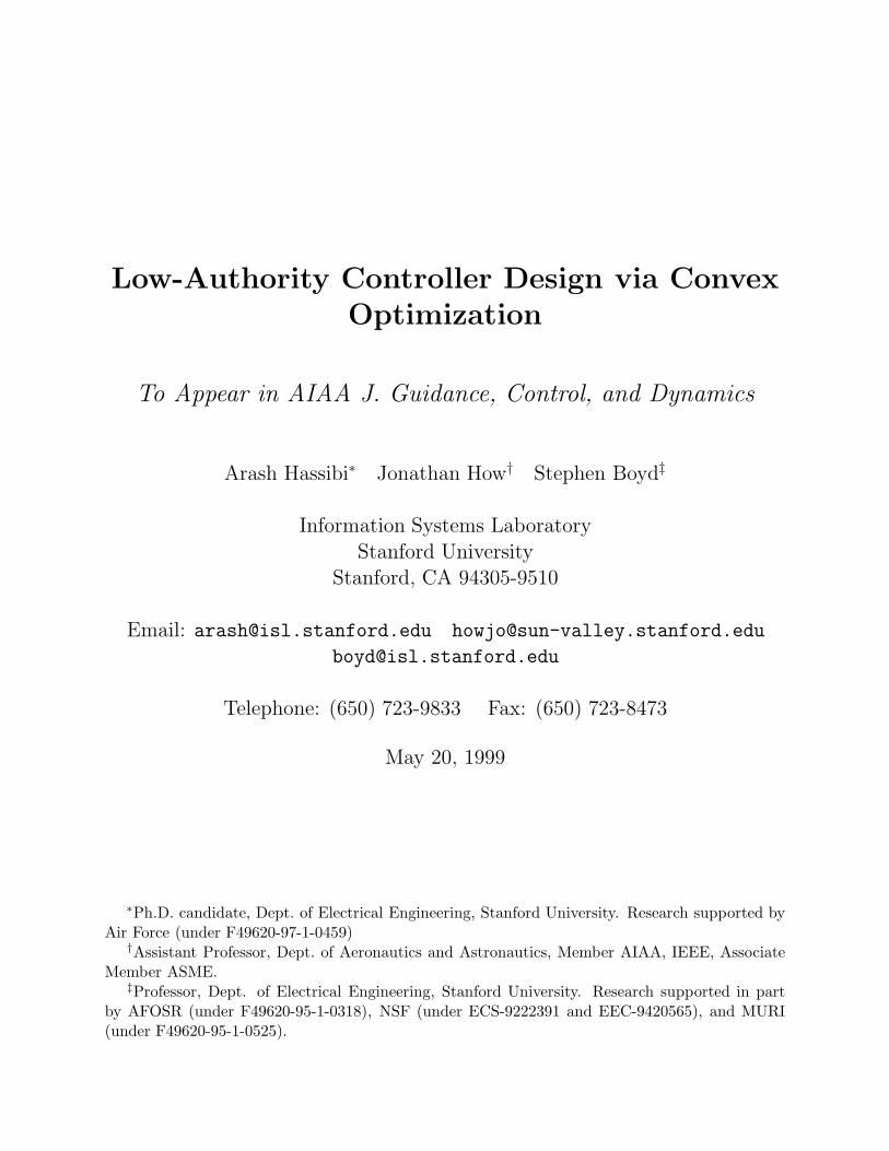
9 Example: LAC design for 39-bar truss structure
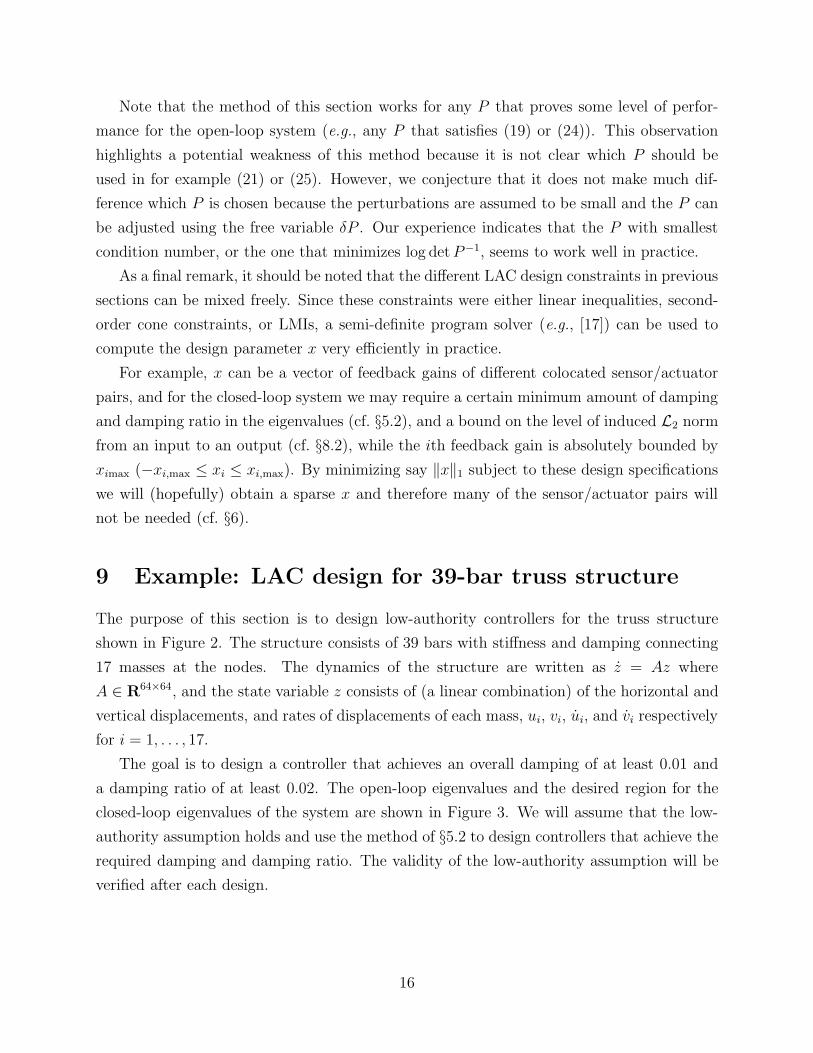
The purpose of this section is to design low-authority controllers for the truss structure
shown in Figure 2. The structure consists of 39 bars with stiffness and damping connecting
17 masses at the nodes. The dynamics of the structure are written as z = Az where
A ∈ R64×64, and the state variable z consists of (a linear combination) of the horizontal and
vertical displacements, and rates of displacements of each mass, ui, vi, ui, and vi respectively
for i = 1, . . . , 17.
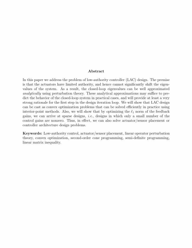
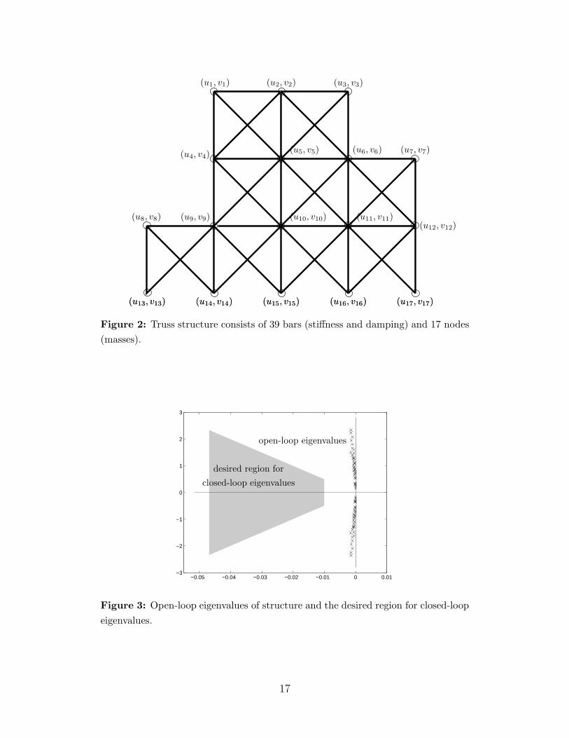
The goal is to design a controller that achieves an overall damping of at least 0.01 and
a damping ratio of at least 0.02. The open-loop eigenvalues and the desired region for the
closed-loop eigenvalues of the system are shown in Figure 3. We will assume that the low-
authority assumption holds and use the method of §5.2 to design controllers that achieve the
required damping and damping ratio. The validity of the low-authority assumption will be
verified after each design.
16
(u1, v1) (u2, v2) (u3, v3)
(u4, v4)(u5, v5) (u6, v6) (u7, v7)
(u8, v8) (u9, v9) (u10, v10) (u11, v11)(u12, v12)
(u13, v13)(u13, v13) (u14, v14)(u14, v14) (u15, v15)(u15, v15) (u16, v16)(u16, v16) (u17, v17)(u17, v17)
Figure 2: Truss structure consists of 39 bars (stiffness and damping) and 17 nodes(masses).
−0.05 −0.04 −0.03 −0.02 −0.01 0 0.01−3
−2
−1
0
1
2
3
desired region forclosed-loop eigenvalues
open-loop eigenvalues
Figure 3: Open-loop eigenvalues of structure and the desired region for closed-loopeigenvalues.
17
9.1 LAC using dampers along bars
We first consider the case in which we can place a damper of size bi along each bar to
achieve the design specifications. The closed-loop system dynamics are now written as
z = A(x)z where the design variables are the size of each of the dampers x = [b1 b2 · · · b39]T
and A(0) = A. In this case, A(x) is affine in x.
It is desirable to find a design in which many of the dampings are zero. To achieve such
a design we minimize the `1 norm of x subject to the eigenvalue placement constraints (note
that the number of sparsity patterns of x is 239 ≈ 1012 and an exhaustive search method
for computing the optimum ‖x‖0 is impractical). The resulting LP that must be solved to
find the damping design consists of 39 variables and 64 linear inequality constraints. The
solution for this problem resulted in 22 out of the 39 possible dampers being zero (this takes
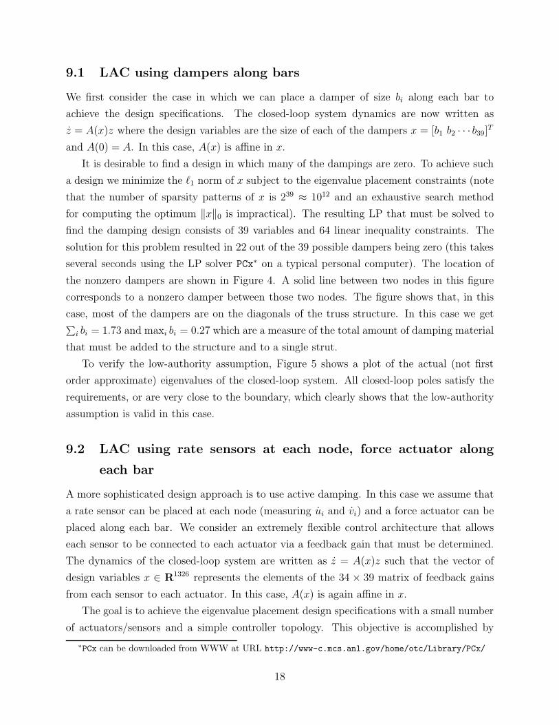
several seconds using the LP solver PCx∗ on a typical personal computer). The location of
the nonzero dampers are shown in Figure 4. A solid line between two nodes in this figure
corresponds to a nonzero damper between those two nodes. The figure shows that, in this
case, most of the dampers are on the diagonals of the truss structure. In this case we get∑i bi = 1.73 and maxi bi = 0.27 which are a measure of the total amount of damping material
that must be added to the structure and to a single strut.
To verify the low-authority assumption, Figure 5 shows a plot of the actual (not first
order approximate) eigenvalues of the closed-loop system. All closed-loop poles satisfy the
requirements, or are very close to the boundary, which clearly shows that the low-authority
assumption is valid in this case.
9.2 LAC using rate sensors at each node, force actuator along
each bar
A more sophisticated design approach is to use active damping. In this case we assume that
a rate sensor can be placed at each node (measuring ui and vi) and a force actuator can be
placed along each bar. We consider an extremely flexible control architecture that allows
each sensor to be connected to each actuator via a feedback gain that must be determined.
The dynamics of the closed-loop system are written as z = A(x)z such that the vector of
design variables x ∈ R1326 represents the elements of the 34 × 39 matrix of feedback gains
from each sensor to each actuator. In this case, A(x) is again affine in x.
The goal is to achieve the eigenvalue placement design specifications with a small number
of actuators/sensors and a simple controller topology. This objective is accomplished by
∗PCx can be downloaded from WWW at URL http://www-c.mcs.anl.gov/home/otc/Library/PCx/
18
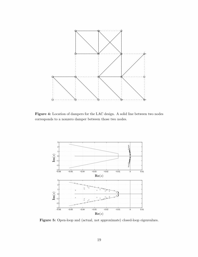
Figure 4: Location of dampers for the LAC design. A solid line between two nodescorresponds to a nonzero damper between those two nodes.
−0.06 −0.05 −0.04 −0.03 −0.02 −0.01 0 0.01−3
−2
−1
0
1
2
3
−0.06 −0.05 −0.04 −0.03 −0.02 −0.01 0 0.01−3
−2
−1
0
1
2
3
Re(s)
Re(s)
Im(s
)Im
(s)
Figure 5: Open-loop and (actual, not approximate) closed-loop eigenvalues.
19
minimizing the `1 norm of x subject to the eigenvalue placement specifications, which is
an LP with 1326 variables and 64 linear inequality constraints (this takes approximately a
minute using PCx on a typical personal computer).
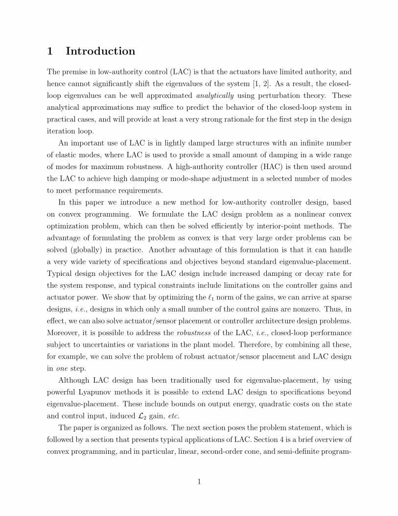
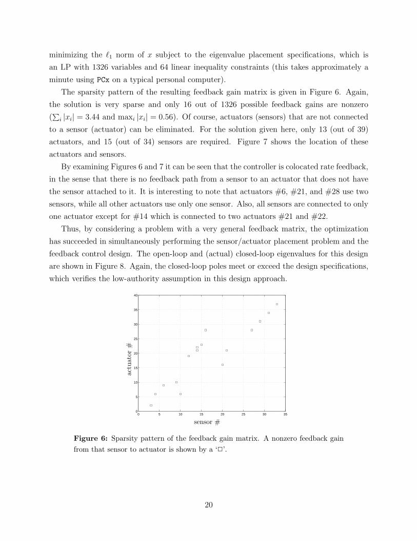
The sparsity pattern of the resulting feedback gain matrix is given in Figure 6. Again,
the solution is very sparse and only 16 out of 1326 possible feedback gains are nonzero
(∑
i |xi| = 3.44 and maxi |xi| = 0.56). Of course, actuators (sensors) that are not connected
to a sensor (actuator) can be eliminated. For the solution given here, only 13 (out of 39)
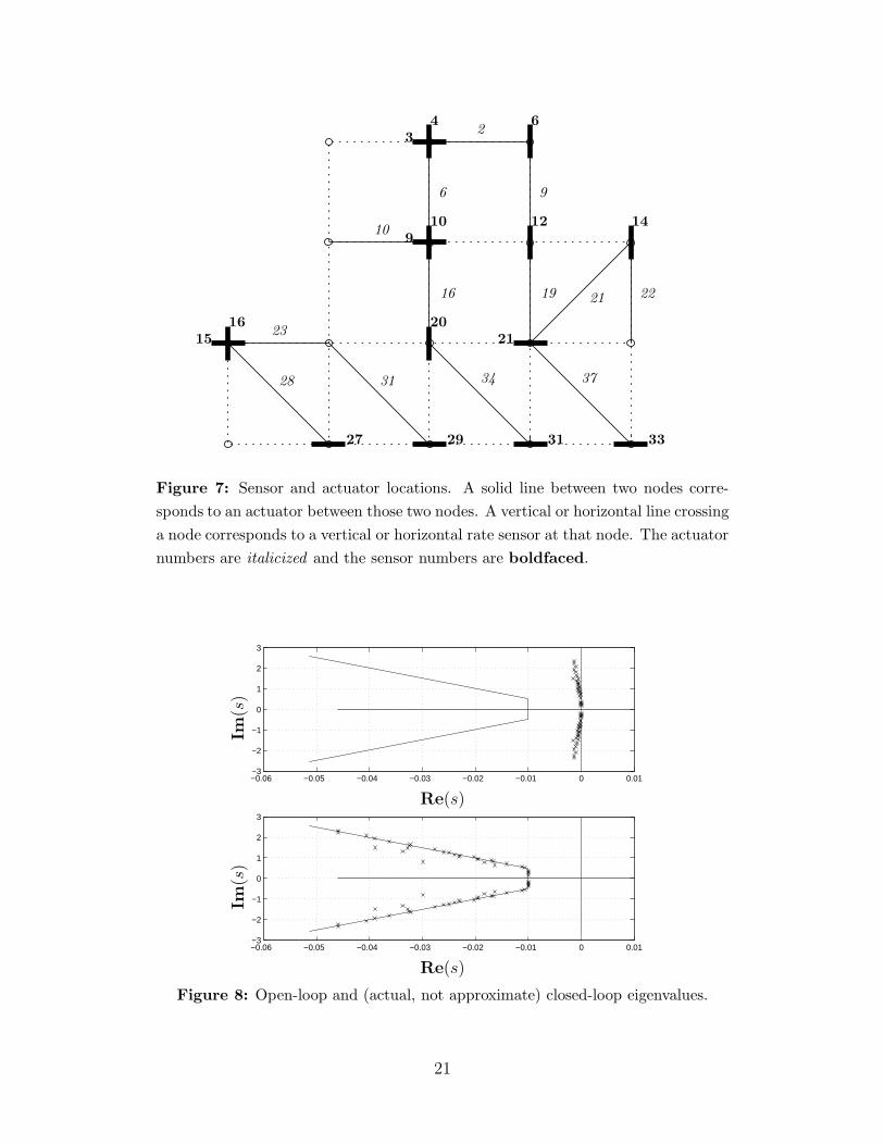
actuators, and 15 (out of 34) sensors are required. Figure 7 shows the location of these
actuators and sensors.
By examining Figures 6 and 7 it can be seen that the controller is colocated rate feedback,
in the sense that there is no feedback path from a sensor to an actuator that does not have
the sensor attached to it. It is interesting to note that actuators #6, #21, and #28 use two
sensors, while all other actuators use only one sensor. Also, all sensors are connected to only
one actuator except for #14 which is connected to two actuators #21 and #22.
Thus, by considering a problem with a very general feedback matrix, the optimization
has succeeded in simultaneously performing the sensor/actuator placement problem and the
feedback control design. The open-loop and (actual) closed-loop eigenvalues for this design
are shown in Figure 8. Again, the closed-loop poles meet or exceed the design specifications,
which verifies the low-authority assumption in this design approach.
0 5 10 15 20 25 30 350
5
10
15
20
25
30
35
40
actu
ator
#
sensor #
Figure 6: Sparsity pattern of the feedback gain matrix. A nonzero feedback gainfrom that sensor to actuator is shown by a ‘2’.
20
2
6 9
10
16 19 21 22
23
28 31 34 37
34 6
910 12 14
1516 20
21
27 29 31 33
Figure 7: Sensor and actuator locations. A solid line between two nodes corre-sponds to an actuator between those two nodes. A vertical or horizontal line crossinga node corresponds to a vertical or horizontal rate sensor at that node. The actuatornumbers are italicized and the sensor numbers are boldfaced.
−0.06 −0.05 −0.04 −0.03 −0.02 −0.01 0 0.01−3
−2
−1
0
1
2
3
−0.06 −0.05 −0.04 −0.03 −0.02 −0.01 0 0.01−3
−2
−1
0
1
2
3
Re(s)
Re(s)
Im(s
)Im
(s)
Figure 8: Open-loop and (actual, not approximate) closed-loop eigenvalues.
21
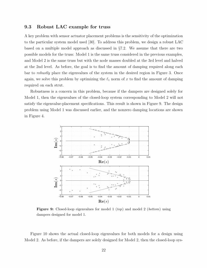
9.3 Robust LAC example for truss
A key problem with sensor actuator placement problems is the sensitivity of the optimization
to the particular system model used [30]. To address this problem, we design a robust LAC
based on a multiple model approach as discussed in §7.2. We assume that there are two
possible models for the truss: Model 1 is the same truss considered in the previous examples,
and Model 2 is the same truss but with the node masses doubled at the 3rd level and halved
at the 2nd level. As before, the goal is to find the amount of damping required along each
bar to robustly place the eigenvalues of the system in the desired region in Figure 3. Once
again, we solve this problem by optimizing the `1 norm of x to find the amount of damping
required on each strut.
Robustness is a concern in this problem, because if the dampers are designed solely for
Model 1, then the eigenvalues of the closed-loop system corresponding to Model 2 will not
satisfy the eigenvalue-placement specifications. This result is shown in Figure 9. The design
problem using Model 1 was discussed earlier, and the nonzero damping locations are shown
in Figure 4.
−0.08 −0.07 −0.06 −0.05 −0.04 −0.03 −0.02 −0.01 0 0.01−3
−2
−1
0
1
2
3
−0.08 −0.07 −0.06 −0.05 −0.04 −0.03 −0.02 −0.01 0 0.01−3
−2
−1
0
1
2
3
Re(s)
Re(s)
Im(s
)Im
(s)
Figure 9: Closed-loop eigenvalues for model 1 (top) and model 2 (bottom) usingdampers designed for model 1.
Figure 10 shows the actual closed-loop eigenvalues for both models for a design using
Model 2. As before, if the dampers are solely designed for Model 2, then the closed-loop sys-
22
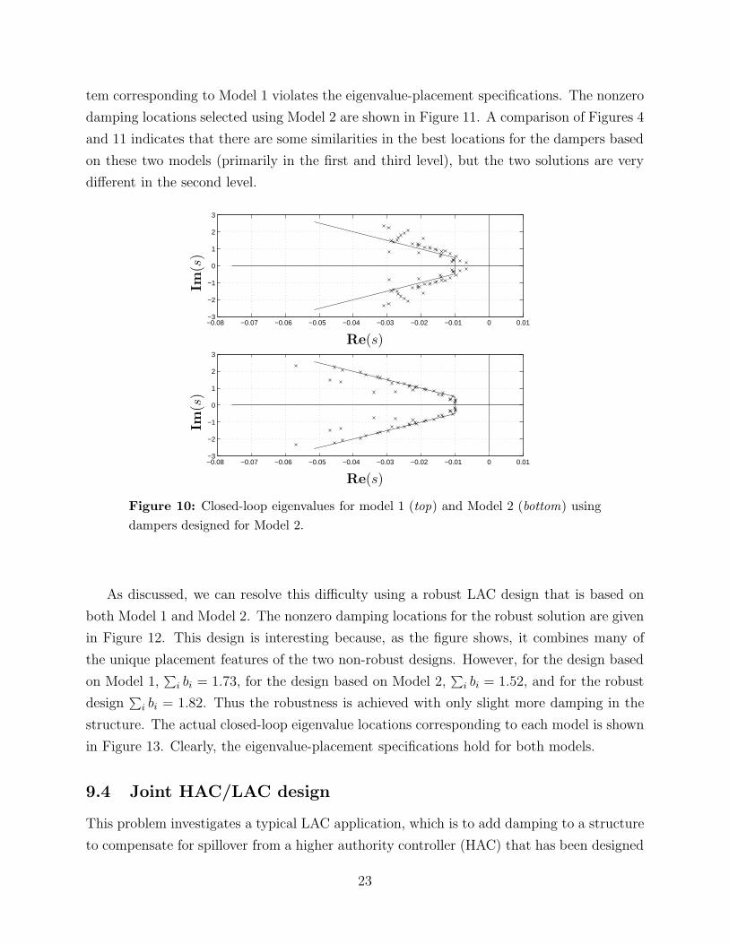
tem corresponding to Model 1 violates the eigenvalue-placement specifications. The nonzero
damping locations selected using Model 2 are shown in Figure 11. A comparison of Figures 4
and 11 indicates that there are some similarities in the best locations for the dampers based
on these two models (primarily in the first and third level), but the two solutions are very
different in the second level.
−0.08 −0.07 −0.06 −0.05 −0.04 −0.03 −0.02 −0.01 0 0.01−3
−2
−1
0
1
2
3
−0.08 −0.07 −0.06 −0.05 −0.04 −0.03 −0.02 −0.01 0 0.01−3
−2
−1
0
1
2
3
Re(s)
Re(s)
Im(s
)Im
(s)
Figure 10: Closed-loop eigenvalues for model 1 (top) and Model 2 (bottom) usingdampers designed for Model 2.
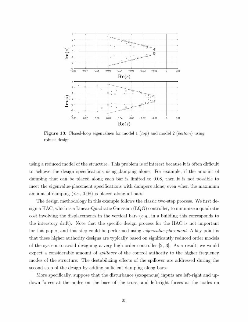
As discussed, we can resolve this difficulty using a robust LAC design that is based on
both Model 1 and Model 2. The nonzero damping locations for the robust solution are given
in Figure 12. This design is interesting because, as the figure shows, it combines many of
the unique placement features of the two non-robust designs. However, for the design based
on Model 1,∑
i bi = 1.73, for the design based on Model 2,∑
i bi = 1.52, and for the robust
design∑
i bi = 1.82. Thus the robustness is achieved with only slight more damping in the
structure. The actual closed-loop eigenvalue locations corresponding to each model is shown
in Figure 13. Clearly, the eigenvalue-placement specifications hold for both models.
9.4 Joint HAC/LAC design
This problem investigates a typical LAC application, which is to add damping to a structure
to compensate for spillover from a higher authority controller (HAC) that has been designed
23
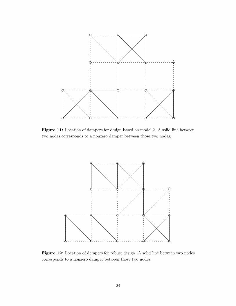
Figure 11: Location of dampers for design based on model 2. A solid line betweentwo nodes corresponds to a nonzero damper between those two nodes.
Figure 12: Location of dampers for robust design. A solid line between two nodescorresponds to a nonzero damper between those two nodes.
24
−0.08 −0.07 −0.06 −0.05 −0.04 −0.03 −0.02 −0.01 0 0.01−3
−2
−1
0
1
2
3
−0.08 −0.07 −0.06 −0.05 −0.04 −0.03 −0.02 −0.01 0 0.01−3
−2
−1
0
1
2
3
Re(s)
Re(s)
Im(s
)Im
(s)
Figure 13: Closed-loop eigenvalues for model 1 (top) and model 2 (bottom) usingrobust design.
using a reduced model of the structure. This problem is of interest because it is often difficult
to achieve the design specifications using damping alone. For example, if the amount of
damping that can be placed along each bar is limited to 0.08, then it is not possible to
meet the eigenvalue-placement specifications with dampers alone, even when the maximum
amount of damping (i.e., 0.08) is placed along all bars.
The design methodology in this example follows the classic two-step process. We first de-
sign a HAC, which is a Linear-Quadratic Gaussian (LQG) controller, to minimize a quadratic
cost involving the displacements in the vertical bars (e.g., in a building this corresponds to
the interstory drift). Note that the specific design process for the HAC is not important
for this paper, and this step could be performed using eigenvalue-placement. A key point is
that these higher authority designs are typically based on significantly reduced order models
of the system to avoid designing a very high order controller [2, 3]. As a result, we would
expect a considerable amount of spillover of the control authority to the higher frequency
modes of the structure. The destabilizing effects of the spillover are addressed during the
second step of the design by adding sufficient damping along bars.
More specifically, suppose that the disturbance (exogenous) inputs are left-right and up-
down forces at the nodes on the base of the truss, and left-right forces at the nodes on
25
the sides of the truss. The output that needs to be regulated is the displacement of the
vertical bars. The actuators for control are force actuators along bars at the first level of
the truss as well as force actuators along vertical bars at other levels. The sensors measure
the displacement of all bars on the highest level of the truss as well as the displacement of
all vertical bars at other levels. (Since the regulating output involves the displacement of
vertical bars it is reasonable to have a sensor/actuator pair along each vertical bar, otherwise
there is no specific reason in choosing the actuator/sensors as such). The LQG controller is
designed based on a reduced-order truss model, using the 5 lowest frequency modes which are
the most lightly damped modes and have a good frequency seperation from the remaining
27 modes. The relative weight of the output energy and control input energy in the LQG
cost were tuned until the HAC provided reasonable performance for the reduced order model
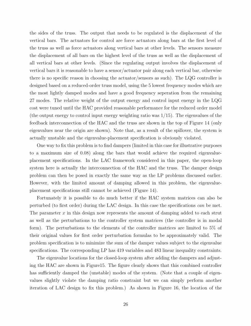
(the output energy to control input energy weighting ratio was 1/15). The eigenvalues of the
feedback interconnection of the HAC and the truss are shown in the top of Figure 14 (only
eigenvalues near the origin are shown). Note that, as a result of the spillover, the system is
actually unstable and the eigenvalue-placement specification is obviously violated.
One way to fix this problem is to find dampers (limited in this case for illustrative purposes
to a maximum size of 0.08) along the bars that would achieve the required eigenvalue-
placement specifications. In the LAC framework considered in this paper, the open-loop
system here is actually the interconnection of the HAC and the truss. The damper design
problem can then be posed in exactly the same way as the LP problems discussed earlier.
However, with the limited amount of damping allowed in this problem, the eigenvalue-
placement specifications still cannot be achieved (Figure 14).
Fortunately it is possible to do much better if the HAC system matrices can also be
perturbed (to first order) during the LAC design. In this case the specifications can be met.
The parameter x in this design now represents the amount of damping added to each strut
as well as the perturbations to the controller system matrices (the controller is in modal
form). The perturbations to the elements of the controller matrices are limited to 5% of
their original values for first order perturbation formulas to be approximately valid. The
problem specification is to minimize the sum of the damper values subject to the eigenvalue
specifications. The corresponding LP has 419 variables and 483 linear inequality constraints.
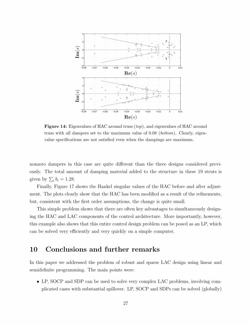
The eigenvalue locations for the closed-loop system after adding the dampers and adjust-
ing the HAC are shown in Figure15. The figure clearly shows that this combined controller
has sufficiently damped the (unstable) modes of the system. (Note that a couple of eigen-
values slightly violate the damping ratio constraint but we can simply perform another
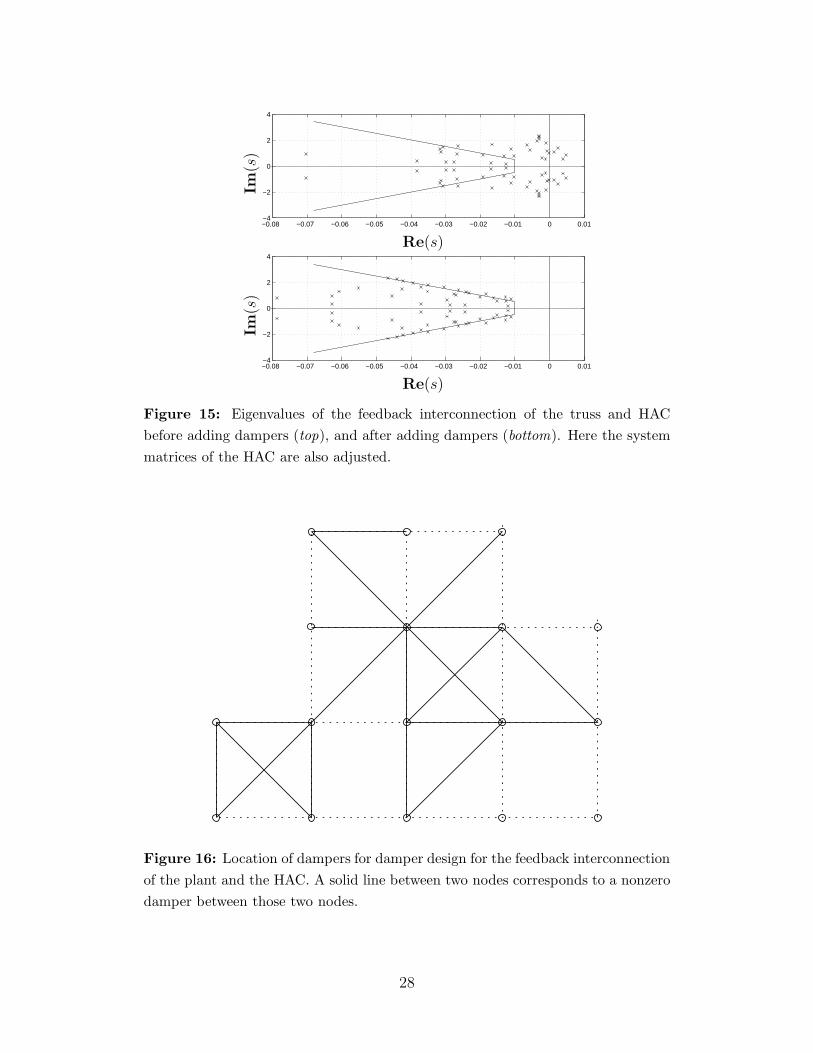
iteration of LAC design to fix this problem.) As shown in Figure 16, the location of the
26
−0.08 −0.07 −0.06 −0.05 −0.04 −0.03 −0.02 −0.01 0 0.01−4
−2
0
2
4
−0.08 −0.07 −0.06 −0.05 −0.04 −0.03 −0.02 −0.01 0 0.01−4
−2
0
2
4
Re(s)
Re(s)
Im(s
)Im
(s)
Figure 14: Eigenvalues of HAC around truss (top), and eigenvalues of HAC aroundtruss with all dampers set to the maximum value of 0.08 (bottom). Clearly, eigen-value specifications are not satisfied even when the dampings are maximum.
nonzero dampers in this case are quite different than the three designs considered previ-
ously. The total amount of damping material added to the structure in these 19 struts is
given by∑
i bi = 1.28.
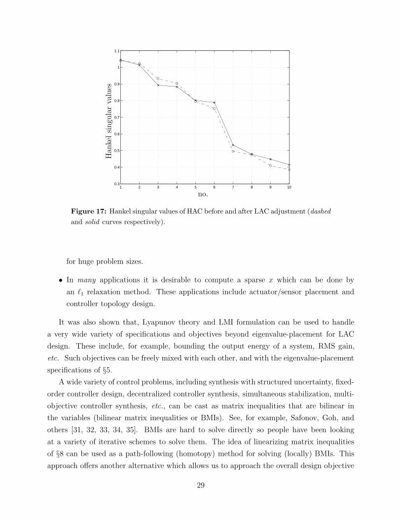
Finally, Figure 17 shows the Hankel singular values of the HAC before and after adjust-
ment. The plots clearly show that the HAC has been modified as a result of the refinements,
but, consistent with the first order assumptions, the change is quite small.
This simple problem shows that there are often key advantages to simultaneously design-
ing the HAC and LAC components of the control architecture. More importantly, however,
this example also shows that this entire control design problem can be posed as an LP, which
can be solved very efficiently and very quickly on a simple computer.
10 Conclusions and further remarks
In this paper we addressed the problem of robust and sparse LAC design using linear and
semidefinite programming. The main points were:
• LP, SOCP and SDP can be used to solve very complex LAC problems, involving com-
plicated cases with substantial spillover. LP, SOCP and SDPs can be solved (globally)
27
−0.08 −0.07 −0.06 −0.05 −0.04 −0.03 −0.02 −0.01 0 0.01−4
−2
0
2
4
−0.08 −0.07 −0.06 −0.05 −0.04 −0.03 −0.02 −0.01 0 0.01−4
−2
0
2
4
Re(s)
Re(s)
Im(s
)Im
(s)
Figure 15: Eigenvalues of the feedback interconnection of the truss and HACbefore adding dampers (top), and after adding dampers (bottom). Here the systemmatrices of the HAC are also adjusted.
Figure 16: Location of dampers for damper design for the feedback interconnectionof the plant and the HAC. A solid line between two nodes corresponds to a nonzerodamper between those two nodes.
28
1 2 3 4 5 6 7 8 9 100.3
0.4
0.5
0.6
0.7
0.8
0.9
1
1.1
Han
kelsi
ngu
lar
valu
es
no.
Figure 17: Hankel singular values of HAC before and after LAC adjustment (dashedand solid curves respectively).
for huge problem sizes.
• In many applications it is desirable to compute a sparse x which can be done by
an `1 relaxation method. These applications include actuator/sensor placement and
controller topology design.
It was also shown that, Lyapunov theory and LMI formulation can be used to handle
a very wide variety of specifications and objectives beyond eigenvalue-placement for LAC
design. These include, for example, bounding the output energy of a system, RMS gain,
etc. Such objectives can be freely mixed with each other, and with the eigenvalue-placement
specifications of §5.
A wide variety of control problems, including synthesis with structured uncertainty, fixed-
order controller design, decentralized controller synthesis, simultaneous stabilization, multi-
objective controller synthesis, etc., can be cast as matrix inequalities that are bilinear in
the variables (bilinear matrix inequalities or BMIs). See, for example, Safonov, Goh, and
others [31, 32, 33, 34, 35]. BMIs are hard to solve directly so people have been looking
at a variety of iterative schemes to solve them. The idea of linearizing matrix inequalities
of §8 can be used as a path-following (homotopy) method for solving (locally) BMIs. This
approach offers another alternative which allows us to approach the overall design objective
29
by iteratively solving a sequence of linearized problems. Starting from the initial (open-
loop) system, the idea is to design better and better controllers by slowly improving the
design objective (e.g., given a reduced-order, decentralized, or fixed architecture controller
could iteratively design for lower values of induced L2 norm). Since the design objective in
consecutive problems are close, at each step, we can linearize the bilinear matrix inequality
to accurately design a controller that is slightly better than the previous one by solving an
SDP.
References
[1] J. H. Wykes. Structural dynamic stability augmentation and gust alleviation of flexible aircraft. InAIAA Paper 68-1067, AIAA Anual Meeting, October 1968.
[2] J. N. Aubrun. Theory of control of structures by low-authority controllers. Journal of Guidance andControl, 3(5):444–451, September 1980.
[3] J. N. Aubrun, N. K. Gupta, and M. G. Lyons. Large space structures control: An integrated approach.In Proceedings of AIAA Guidance and Control Conference, Boulder, Colorado, August 1979.
[4] T. Williams. Transmission zeros and high-authority/low-authority control of flexible space structures.Journal of Guidance, Control, and Dynamics, 17(1):170–4, January 1994.
[5] C. T. Sun and Y. P. Lu. Vibration Damping of Structural Elements. Prentice Hall, 1995.
[6] R. J. Vanderbei. Linear Programming: Foundations and Extensions. Kluwer Academic Publishers,1997.
[7] Yu. Nesterov and A. Nemirovsky. Interior-point polynomial methods in convex programming, volume 13of Studies in Applied Mathematics. SIAM, Philadelphia, PA, 1994.
[8] L. Vandenberghe and S. Boyd. A primal-dual potential reduction method for problems involving matrixinequalities. Mathematical Programming, 69(1):205–236, July 1995.
[9] L. A. Zadeh and B. H. Whalen. On optimal control and linear programming. IRE Transactions onAutomatic Control, pages 45–6, July 1962.
[10] J. Richalet. Industrial applications of model based predictive control. Automatica, 29(5):1251–1274,1993.
[11] R. J. Vanderbei. LOQO user’s manual. Technical Report SOL 92–05, Dept. of Civil Engineering andOperations Research, Princeton University, Princeton, NJ 08544, USA, 1992.
[12] Y. Zhang. User’s guide to LIPSOL: a matlab toolkit for linear programming interior-point solvers.Math. & Stat. Dept., Univ. Md. Baltimore County, October 1994. Beta release.
[13] J. Czyzyk, S. Mehrotra, and S. J. Wright. PCx User Guide. Optimization Technology Cneter, March1997.
[14] F. Alizadeh, J.-P. Haeberly, and M. Overton. A new primal-dual interior-point method for semidefiniteprogramming. In Proceedings of the Fifth SIAM Conference on Applied Linear Algebra, Snowbird, Utah,June 1994.
[15] L. Vandenberghe and S. Boyd. sp: Software for Semidefinite Programming. User’s Guide, Beta Version.Stanford University, October 1994. Available at http://www-isl.stanford.edu/people/boyd.
[16] K. Fujisawa and M. Kojima. SDPA (semidefinite programming algorithm) user’s manual. TechnicalReport B-308, Department of Mathematical and Computing Sciences. Tokyo Institute of Technology,1995.
30
[17] S.-P. Wu and S. Boyd. sdpsol: A Parser/Solver for Semidefinite Programming and DeterminantMaximization Problems with Matrix Structure. User’s Guide, Version Beta. Stanford University, June1996.
[18] P. Gahinet and A. Nemirovskii. LMI Lab: A Package for Manipulating and Solving LMIs. INRIA,1993.
[19] F. Alizadeh, J. P. Haeberly, M. V. Nayakkankuppam, and M. L. Overton. sdppack User’s Guide,Version 0.8 Beta. NYU, June 1997.
[20] B. Borchers. csdp, a C library for semidefinite programming. New Mexico Tech, March 1997.
[21] S. Boyd, L. El Ghaoui, E. Feron, and V. Balakrishnan. Linear Matrix Inequalities in System and ControlTheory, volume 15 of Studies in Applied Mathematics. SIAM, Philadelphia, PA, June 1994.
[22] M. S. Lobo, L. Vandenberghe, S. Boyd, and H. Lebret. Applications of second-order cone programming.Linear Algebra and Applications, 284(1-3):193–228, November 1998.
[23] M. S. Lobo, L. Vandenberghe, and S. Boyd. socp: Software for Second-Order Cone Programming.Information Systems Laboratory, Stanford University, 1997.
[24] F. Alizadeh, J. P. Haeberly, M. V. Nayakkankuppam, M. L. Overton, and S. Schmieta. sdppack User’sGuide, Version 0.9 Beta. NYU, June 1997.
[25] T. Kato. A Short Introduction to Perturbation Theory for Linear Operators. Springer-Verlag, 1982.
[26] S. S. Chen, D. Donoho, and M. A. Saunders. Atomic decomposition of basis pursuit. Technical report,Dept. of Statistics, Stanford University, February 1996.
[27] B. D. Rao and I. F. Gorodnitsky. Affine scaling transformation based methods for computing lowcomplexity sparse solutions. In Proceedings of IEEE International Conference on Acoustics, Speech,and Signal Processing, volume 3, pages 1783–6, Atlanta, GA, May 1996.
[28] G. Harikumar and Y. Bresler. A new algorithm for computing sparse solutions to linear inverse problems.In Proc. ICASSP 96, pages 1331–1334, May 1996.
[29] M. Mesbahi and G. P. Papavassilopoulos. On the rank minimization problem over a positive semidefinitelinear matrix inequality. IEEE Transactions on Automatic Control, AC-42(2):239–43, February 1997.
[30] E. H. Anderson and N. W. Hagood. Robust placement of actuators and dampers for structural control.Technical Report of the Space Engineering Research Center SERC#14-93, Massachusetts Institute ofTechnology, October 1993.
[31] K. C. Goh, M. G. Safonov, and G. P. Papavassilopoulos. A global optimization approach for the BMIproblem. In Proceedings of IEEE Conference on Decision and Control, volume 4, pages 2009–14, LakeBuena Vista, FL, December 1994.
[32] M. G. Safonov, K. C. Goh, and J. H. Ly. Control system synthesis via bilinear matrix inequalities. InProceedings of American Control Conference, volume 1, pages 45–9, Baltimore, MD, 1994.
[33] K. C. Goh, L. Turan, M. G. Safonov, G. P. Papavassilopoulos, and J. H. Ly. Biaffine matrix inequalityproperties and computational methods. In Proc. American Control Conf., pages 850–855, 1994.
[34] K.-C. Goh. Robust Control Synthesis via Bilinear Matrix Inequalities. PhD thesis, University of SouthernCalifornia, May 1995.
[35] M. Mesbahi, G. P. Papavassilopoulos, and M. G. Safonov. Matrix cones, complementarity problems andthe bilinear matrix inequality. In Proceedings of IEEE Conference on Decision and Control, volume 3,pages 3102–7, New Orleans, LA, 1995.
31