Low-AngleRadar Land

ClutterMeasurements and

Empirical Models

J. Barrie BillingsleyLincoln Laboratory

Massachusetts Instituteof Technology

William Andrew Publishing

Published in the United States of America by William Andrew Publishing / Noyes Publishing13 Eaton AvenueNorwich, NY 13815www.williamandrew.com

President and CEO: William WoishnisSponsoring Editor: Dudley R. Kay – SciTech Publishing, Inc.Production Manager: Kathy BreedProduction services provided by TIPS Technical Publishing, Carrboro, North Carolina

Copyeditor: Howard JonesBook Design: Robert KernCompositor: Lynanne FowleProofreaders: Maria Mauriello, Jeff Eckert

Printed in the United States

10 9 8 7 6 5 4 3 2 1

Copyright © 2002 by William Andrew Publishing, Inc.No part of this book may be reproduced or utilized in any form or by any means, electronic or mechanical, including photocopying, recording or by any information storage and retrieval system, without permission in writing from the Publisher.

SciTech is a partner with William Andrew for high-quality radar and aerospace books.See www.scitechpub.com for information.

Library of Congress Cataloging-in-Publication DataBillingsley, J. Barrie.

Low angle radar land clutter : measurements and empirical models / J. Barrie Billingsley.p. cm.

Includes index.ISBN 1-891121-16-2 (alk. paper)1. Radar—Interference. I. Title

TK6580 .B45 2001621.3848—dc21

2001034284

This book is co-published and distributed in the UK and Europe by:

The Institution of Electrical EngineersMichael Faraday HouseSix Hills Way, Stevenage, SGI 2AY, UKPhone: +44 (0) 1438 313311Fax: +44 (0) 1438 313465Email: books@iee.org.ukwww.iee.org.uk/publishIEE ISBN: 0-85296-230-4

Other Books Under the SciTech Imprint

How to Speak Radar CD-Rom (2001)Arnold Acker

Air and Spaceborne Radar Systems: An Introduction (2001)Philippe Lacomme, Jean-Philippe Hardange,

Jean-Claude Marchais, and Eric Normant

Introduction to Airborne Radar, Second Edition (1998)George W. Stimson

Radar Principles for the Non-Specialist, Second Edition (1998)John C. Toomay

Radar Design Principles, Second Edition (1998)Fred Nathanson

Understanding Radar Systems (1998)Simon Kingsley and Shaun Quegan

Hazardous Gas Monitors (2000)Jack Chou

The Advanced Communication Satellite System (2000)Richard Gedney, Ronald Shertler, and Frank Gargione

Moving Up the Organization in Facilities ManagementA. S. Damiani

Return of the Ether (1999)Sid Deutsch

To my wife Mary, and to our children Jennifer, Michael, and Thomas,

and grandchildren Andrew and Sylvia

Foreword

MIT Lincoln Laboratory was founded in 1951 to develop a strategic air-defense system forthe United States. The Laboratory engineers of that era quickly found that ground cluttergreatly limited the performance of their radars. Consequently, they pioneered thedevelopment of Doppler processing techniques and later digital processing techniques tomitigate the effects of ground clutter. The Laboratory returned to the problem of airdefense in the late 1970s with a major program to assess and ensure the survivability ofU.S. cruise missiles. Once again ground clutter proved an important issue because a low-flying, low-observable cruise missile could hide in ground clutter and escape radardetection. The new challenge was to confidently predict low-grazing angle ground clutterfor any number of specific sites with widely varying topographies. But the understandingof clutter phenomena at this time certainly did not permit these predictions. Therefore,with the early support of the Defense Advanced Research Projects Agency and later withthe support of the United States Air Force, the Laboratory set out to make a majorimprovement in our understanding of ground clutter as seen by ground radars.

Barrie Billingsley was the principal researcher at the start and I was the director of theoverall Laboratory program. I recall telling Barrie to archive his data, document hisexperiments, calibrate his radars, and collect ground truth on his many test sites so that hecould write the definitive textbook on low grazing angle ground clutter when our programwas finished. I would say that Barrie has delivered magnificently on this challenge. I amdelighted to see over 300 directly applicable charts characterizing ground clutterbackscatter in this book.

I confess that I had expected this book to appear about 10 years after the start, not 20 years.The long gestation period reflects the enormous technical problem of capturing what reallyhappens at low grazing angles and the fact that Barrie Billingsley is an extremelymeticulous and persistent researcher. He did stretch the patience of successive LincolnLaboratory program managers, but he pulled it off by teasing us each year with additionalinsights into these complex clutter phenomena. We greatly admired his research abilitiesand his dedication to the task of unfolding the mystery of low grazing angle ground clutter.We had heard the violins and the horns and the woodwinds before, but now we couldunderstand the whole orchestration—how frequency, terrain, propagation, resolution, andpolarization all operated together to produce the complex result we had witnessed but didnot understand.

My congratulations to Barrie for this grand accomplishment—a book that will serveengineers and scientists for many years to come. My congratulations also to hiscollaborators and the long sequence of Lincoln Laboratory program managers whosupported Barrie in this most important endeavor. My thanks to the Defense AdvancedResearch Projects Agency and United States Air Force for their enlightened support andmanagement of this program. It is not very often in the defense research business that weget to complete and beautifully wrap a wonderful piece of scientific research. Enjoy!

— William P. DelaneyPine Island, Meredith, New Hampshire

November 2001

Preface

Radar land clutter constitutes the unwanted radar echoes returned from the earth’s surfacethat compete against and interfere with the desired echoes returned from targets ofinterest, such as aircraft or other moving or stationary objects. To be able toknowledgeably design and predict the performance of radars operating to providesurveillance of airspace, detection and tracking of targets, and other functions in landclutter backgrounds out to the radar horizon, radar engineers require accurate descriptionsof the strengths of the land clutter returns and their statistical attributes as they vary frompulse to pulse and cell to cell. The problem of bringing statistical order and predictabilityto land clutter is particularly onerous at the low angles (at or near grazing incidence) atwhich surface-sited radars illuminate the clutter-producing terrain, where the fundamentaldifficulty arising from the essentially infinite variability of composite terrain isexacerbated by such effects as specularity against discrete clutter sources and intermittentshadowing. Thus, predicting the effects of low-angle land clutter in surface radar was formany years a major unsolved problem in radar technology.

Based on the results of a 20-year program of measuring and investigating low-angle landclutter carried out at Lincoln Laboratory, Massachusetts Institute of Technology, this bookadvances the state of understanding so as to “solve the low-angle clutter problem” in manyimportant respects. The book thoroughly documents all important results of the LincolnLaboratory clutter program. These results enable the user to predict land clutter effects insurface radar.

This book is comprehensive in addressing the specific topic of low-angle land clutterphenomenology. It contains many interrelated results, each important in its own right, andunifies and integrates them so as to add up to a work of significant technological innovationand consequence. Mean clutter strength is specified for most important terrain types (e.g.,forest, farmland, mountains, desert, urban, etc.). Information is also provided specifyingthe statistical distributions of clutter strength, necessary for determining probabilities ofdetection and false alarm against targets in clutter backgrounds. The totality of cluttermodeling information so presented is parameterized, not only by the type of terrain givingrise to the clutter returns, but also (and importantly) by the angle at which the radarilluminates the ground and by such important radar parameters as carrier frequency, spatialresolution, and polarization. This information is put forward in terms of empirical cluttermodels. These include a Weibull statistical model for prediction of clutter strength and anexponential model for the prediction of clutter Doppler spreading due to wind-inducedintrinsic clutter motion. Also included are analyses and results indicating, given thestrength and spreading of clutter, to what extent various techniques of clutter cancellationcan reduce the effects of clutter on target detection performance.

The empirically-derived clutter modeling information thus provided in this book utilizeseasy-to-understand formats and easy-to-implement models. Each of the six chapters isessentially self-contained, although reading them consecutively provides an iterativepedagogical approach that allows the ideas underlying the finalized modeling informationof Chapters 5 and 6 to be fully explored. No difficult mathematics exist to prevent easy

xvi Preface

assimilation of the subject matter of each chapter by the reader. The technical writing styleis formal and dedicated to maximizing clarity and conciseness of presentation. Meticulousattention is paid to accuracy, consistency, and correctness of results. No further prerequisiterequirements are necessary beyond the normal knowledge base of the working radarengineer (or student) to access the information of this book. A fortuitous combination ofnational political, technological, and economic circumstances occurring in the late 1970sand early 1980s allowed the Lincoln Laboratory land clutter measurement project to beimplemented and thereafter continued in studies and analysis over a 20-year period. It ishighly unlikely that another program of the scope of the Lincoln Laboratory clutterprogram will take place in the foreseeable future. Future clutter measurement programs areexpected to build on or extend the information of this book in defined specific directions,rather than supersede this information. Thus this book is expected to be of long-lastingsignificance and to be a definitive work and standard reference on the subject of land clutterphenomenology.

A number of individuals and organizations provided significant contributions to the PhaseZero/Phase One land clutter measurements and modeling program at Lincoln Laboratoryand consequently towards bringing this book into existence and affecting its final form andcontents. This program commenced at Lincoln Laboratory in 1978 under sponsorship fromthe Defense Advanced Research Projects Agency. The United States Air Force began jointsponsorship several years into the program and subsequently assumed full sponsorship overthe longer period of its complete duration. The program was originally conceived by Mr.William P. Delaney of Lincoln Laboratory, and largely came into focus in a short 1977DARPA/USAF-sponsored summer study requested by the Department of Defense anddirected by Mr. Delaney. The Phase Zero/Phase One program was first managed at LincolnLaboratory by Mr. Carl E. Nielsen Jr. and by Dr. David L. Briggs, and subsequently by Dr.Lewis A. Thurman and Dr. Curtis W. Davis III.

Early site selection studies for the Phase Zero/Phase One program indicated the desirabilityof focusing measurements in terrain of relatively low relief and at northern latitudes such asgenerally occurs in the prairie provinces of western Canada. As a result, a Memorandum ofUnderstanding (MOU) was established between the United States and Canadaimplementing a joint clutter measurements program in which Canada, through DefenceResearch Establishment Ottawa, was to provide logistics support and share in the measureddata and results. Dr. Hing C. Chan was the principal investigator of the clutter data atDREO. Dr. Chan became a close and valued member of the Phase One community; manyuseful discussions and interactions concerning the measured clutter data and its analysisoccurred between Dr. Chan and the author down to the time of present writing. Substantialcontracted data analysis support activity was provided to Dr. Chan by AIT Corporation,Ottawa. Information descriptive of the terrain at the clutter measurement sites was providedin a succession of contracted studies at Intera Information Technologies Ltd., Calgary.

The government of the United Kingdom through its Defence Evaluation Research Agencybecame interested in the Lincoln Laboratory clutter program shortly after itscommencement. DERA subsequently became involved in the analysis of Phase One clutterdata under the aegis of The Technical Cooperation Program (TTCP), an internationaldefense science technical information exchange program. The U.S./Canada MOU wasterminated at the completion of measurements, and the sharing of the measurement dataand its analysis was thereafter continued between all three countries under TTCP.

Preface xvii

Significant analyses of selected subsets of the Phase One measurement data occurred withDERA sponsorship in the U.K. at Smith Associates Limited and at GEC Marconi ResearchCentre. The principal coordinator of these interactions at DERA was Mr. Robert A.Blinston. Mr. John N. Entzminger Jr., former Director of the Tactical Technology Office atDARPA, provided much encouragement to these joint U.S./Canada/U.K. clutter studyinteractions in his role as head of the U.S. delegation to Subgroup K (radar) in TTCP.

In its early years, the Lincoln Laboratory clutter program was followed by Mr. David K.Barton, then of Raytheon Company, now of ANRO Engineering, who stimulated ourthinking with his insights on the interrelationships of clutter and propagation anddiscussions on approaches to clutter modeling. Also in the early years of the clutterprogram, several interactions with Mr. William L. Simkins of the Air Force ResearchLaboratory, Rome, N.Y., influenced methodology to develop correctly at LincolnLaboratory in such matters as clutter data reduction and intrinsic-motion clutter spectralmodeling. In the latter years of the Phase One program, Professor Alfonso Farina of AleniaMarconi Systems, Italy, became interested in the clutter data. An informal collaborationwas organized by Professor Farina in which some particular Phase One clutter data setswere provided to and studied by him and his colleagues at the University of Pisa andUniversity of Rome. These studies were from the point of view of signal processing andtarget detectability in ground clutter backgrounds. A number of jointly-authored technicaljournal papers in the scientific literature resulted.

The five-frequency Phase One clutter measurement equipment was fabricated by the GeneralElectric Co., Syracuse, N.Y. (now part of Lockheed Martin Corporation). Key members ofthe Phase One measurements crew were Harry Dence and Joe Miller of GE, Captain KenLockhart of the Canadian Forces, and Jerry Anderson of Intera. At Lincoln Laboratory, theprincipal people involved in the management and technical interface with GE were DavidKettner and John Hartt. The project engineer of the precursor X-band Phase Zero clutterprogram was Ovide Fortier. People who had significant involvement in data reduction andcomputer programming activities include Gerry McCaffrey, Paul Crochetiere, Ken Gregson,Peter Briggs, Bill Dustin, Bob Graham-Munn, Carol Bernhard, Kim Jones, Charlotte Schell,Louise Moss, and Sharon Kelsey. Dr. Seichoong Chang served in an important consultantrole in overseeing the accurate calibration of the clutter data. Many informative discussionswith Dr. Serpil Ayasli helped provide understanding of the significant effects ofelectromagnetic propagation in the clutter data. Application of the resultant clutter models inradar system studies took place under the jurisdiction of Dr. John Eidson.

The original idea that the results of the Lincoln Laboratory clutter program could be thebasis of a clutter reference book valuable to the radar community at large came from Mr.Delaney. Dr. Merrill I. Skolnik, former Superintendent of the Radar Division at the NavalResearch Laboratory in Washington, D.C., lent his support to this book idea and providedencouragement to the author in his efforts to follow through with it. When a first roughdraft of Chapter 1 of the proposed book became available, Dr. Skolnik kindly read it andprovided a number of constructive suggestions. Throughout the duration of the clutter bookproject, Dr. Thurman was a never-failing source of positive managerial support andinsightful counsel to the author on how best to carry the book project forward. Mr. C.E.Muehe provided a thorough critical review of the original report material upon which muchof Chapter 6 is based. Dr. William E. Keicher followed the book project in its later stagesand provided a technical review of the entire book manuscript. Skillful typing of the

xviii Preface

original manuscript of this book was patiently and cheerfully performed through its manyiterations by Gail Kirkwood. Pat DeCuir typed many of the original technical reports uponwhich the book is largely based. Members of the Lincoln Laboratory Publications groupmaintained an always positive and most helpful approach in transforming the originalrough manuscript into highly finished form. These people in particular include DeborahGoodwin, Jennifer Weis, Dorothy Ryan, and Katherine Shackelford. Dudley R. Kay,president of SciTech Publishing and vice-president at William Andrew Publishing, and thebook’s compositors, Lynanne Fowle and Robert Kern at TIPS Technical Publishing, ablyand proficiently met the many challenges in successfully seeing the book to press.

It is a particular pleasure for the author to acknowledge the dedicated and invaluableassistance provided by Mr. John F. Larrabee (Lockheed Martin Corporation) in the day-to-day management, reduction, and analyses of the clutter data at Lincoln Laboratory over thefull duration of the project. In the latter days of the clutter project involving the productionof this book, Mr. Larrabee managed the interface to the Lincoln Laboratory Publicationsgroup and provided meticulous attention to detail in the many necessary iterations requiredin preparing all the figures and tables of the book. Mr. Larrabee recently retired after a longprofessional career in contracted employment at Lincoln Laboratory, at about the time thebook manuscript was being delivered to the publisher.

Many others contributed to the land clutter project at Lincoln Laboratory. Lack of explicitmention here does not mean that the author is not fully aware of the value of eachcontribution or lessen the debt of gratitude owed to everyone involved in acquiring,reducing, and analyzing the clutter data. Although this book was written at LincolnLaboratory, Massachusetts Institute of Technology, under the sponsorship of DARPA andthe USAF, the opinions, recommendations, and conclusions of the book are those of theauthor and are not necessarily endorsed by the sponsoring agencies. Permissions receivedfrom the Institute of Electrical and Electronics Engineers, Inc., the Institution of ElectricalEngineers (U.K.), and The McGraw-Hill Companies to make use of copyrighted materialsare gratefully acknowledged. Any errors or shortcomings that remain in the material of thebook are entirely the responsibility of the author. The author sincerely hopes that everyreader of this book is able to find helpful information within its pages.

— J. Barrie BillingsleyLexington, Massachusetts

October 2001

Contents

Foreword xiiiPreface xv

Chapter 1 Overview 1

1.1 Introduction 11.2 Historical Review 3

1.2.1 Constant σ ° 41.2.2 Wide Clutter Amplitude Distributions 51.2.3 Spatial Inhomogeneity/Resolution Dependence 61.2.4 Discrete Clutter Sources 81.2.5 Illumination Angle 91.2.6 Range Dependence 111.2.7 Status 13

1.3 Clutter Measurements at Lincoln Laboratory 131.4 Clutter Prediction at Lincoln Laboratory 16

1.4.1 Empirical Approach 171.4.2 Deterministic Patchiness 181.4.3 Statistical Clutter 181.4.4 One-Component σ ° Model 181.4.5 Depression Angle 191.4.6 Decoupling of Radar Frequency and Resolution 201.4.7 Radar Noise Corruption 21

1.5 Scope of Book 231.5.1 Overview 231.5.2 Two Basic Trends 241.5.3 Measurement-System-Independent Clutter Strength 241.5.4 Propagation 241.5.5 Statistical Issues 251.5.6 Simpler Models 261.5.7 Parameter Ranges 26

1.6 Organization of Book 27References 30

Chapter 2 Preliminary X-Band Clutter Measurements 35

2.1 Introduction 352.1.1 Outline 35

2.2 Phase Zero Clutter Measurements 362.2.1 Radar Instrumentation 362.2.2 Measurement Sites 372.2.3 Terrain Description 37

viii Contents

2.3 The Nature of Low-Angle Clutter 422.3.1 Clutter Physics I 422.3.2 Measured Land Clutter Maps 442.3.3 Clutter Patches 462.3.4 Depression Angle 552.3.5 Terrain Slope/Grazing Angle 622.3.6 Clutter Modeling 65

2.4 X-Band Clutter Spatial Amplitude Statistics 682.4.1 Amplitude Distributions by Depression

Angle for Three General Terrain Types 682.4.2 Clutter Results for More Specific Terrain Types 772.4.3 Combining Strategies 962.4.4 Depression Angle Characteristics 1012.4.5 Effect of Radar Spatial Resolution 1102.4.6 Seasonal Effects 111

2.5 Summary 115References 116Appendix 2.A Phase Zero Radar 118Appendix 2.B Formulation of Clutter Statistics 126

Reference 138Appendix 2.C Depression Angle Computation 139

Reference 141

Chapter 3 Repeat Sector Clutter Measurements 143

3.1 Introduction 1433.1.1 Outline 144

3.2 Multifrequency Clutter Measurements 1453.2.1 Equipment and Schedule 1463.2.2 Data Collection 1463.2.3 Terrain Description 156

3.3 Fundamental Effects in Low-Angle Clutter 1603.3.1 Clutter Physics II 1603.3.2 Trends with Radar Frequency 1623.3.3 Depression Angle and Terrain Slope 165

3.4 Mean Land Clutter Strength vs Frequency by Terrain Type 1683.4.1 Detailed Discussion of Measurements 1693.4.2 Twelve Multifrequency Clutter Strength

Characteristics 2043.5 Dependencies of Mean Land Clutter Strength

with Radar Parameters 2093.5.1 Frequency Dependence 2093.5.2 Polarization Dependence 2123.5.3 Resolution Dependence 216

3.6 Higher Moments and Percentiles in Measured Land

Contents ix

Clutter Spatial Amplitude Distributions 2223.6.1 Ratio of Standard Deviation-to-Mean 2223.6.2 Skewness and Kurtosis 2273.6.3 Fifty-, 70-, and 90-Percentile Levels 228

3.7 Effects of Weather and Season 2313.7.1 Diurnal Variability 2343.7.2 Six Repeated Visits 2353.7.3 Temporal and Spatial Variation 237

3.8 Summary 242References 246Appendix 3.A Phase One Radar 247Appendix 3.B Multipath Propagation 259

References 272Appendix 3.C Clutter Computations 274

Chapter 4 Approaches to Clutter Modeling 285

4.1 Introduction 2854.1.1 Modeling Objective 2874.1.2 Modeling Rationale 2884.1.3 Modeling Scope 291

4.2 An Interim Angle-Specific Clutter Model 2924.2.1 Model Basis 2924.2.2 Interim Model 2944.2.3 Error Bounds 297

4.3 Non-Angle-Specific Modeling Considerations 2994.3.1 Phase Zero Results 2994.3.2 Simple Clutter Model 3024.3.3 Further Considerations 3054.3.4 Summary 309

4.4 Terrain Visibility and Clutter Occurrence 3124.4.1 Effects of Trees on Visibility at Cold Lake 3124.4.2 Decreasing Shadowing with Increasing

Site Height 3154.4.3 Vertical Objects on Level Terrain at Altona 3174.4.4 Summary 319

4.5 Discrete vs Distributed Clutter 3204.5.1 Introduction 3204.5.2 Discrete Clutter Sources at Cochrane 3244.5.3 Separation of Discrete Source at Suffield 3254.5.4 σ vs σ ° Normalization 3304.5.5 Conclusions 333

4.6 Temporal Statistics, Spectra, and Correlation 3344.6.1 Temporal Statistics 3354.6.2 Spectral Characteristics 3354.6.3 Correlative Properties 338

x Contents

4.7 Summary 343References 347Appendix 4.A Clutter Strength vs Range 350Appendix 4.B Terrain Visibility as a Function of

Site Height and Antenna Mast Height 359Appendix 4.C Effects of Terrain Shadowing and

Finite Sensitivity 371Appendix 4.D Separation of Discretes in

Clutter Modeling 396

Chapter 5 Multifrequency Land Clutter Modeling Information 407

5.1 Introduction 4075.1.1 Review 408

5.2 Derivation of Clutter Modeling Information 4165.2.1 Weibull Statistics 4165.2.2 Clutter Model Framework 4185.2.3 Derivation of Results 420

5.3 Land Clutter Coefficients for General Terrain 4295.3.1 General Mixed Rural Terrain 4295.3.2 Further Reduction 4375.3.3 Validation of Clutter Model Framework 4395.3.4 Simplified Clutter Prediction 440

5.4 Land Clutter Coefficients for Specific Terrain Types 4405.4.1 Urban or Built-Up Terrain 4435.4.2 Agricultural Terrain 4925.4.3 Forest Terrain 5065.4.4 Shrubland Terrain 5185.4.5 Grassland Terrain 5215.4.6 Wetland Terrain 5265.4.7 Desert Terrain 5295.4.8 Mountainous Terrain 537

5.5 PPI Clutter Map Prediction 5425.5.1 Model Validation 5435.5.2 Model Improvement 543

5.6 Summary 544References 546Appendix 5.A Weibull Statistics 548

References 573

Chapter 6 Windblown Clutter Spectral Measurements 575

6.1 Introduction 5756.2 Exponential Windblown Clutter Spectral Model 576

6.2.1 ac Spectral Shape 577

Contents xi

6.2.2 dc/ac Ratio 5796.2.3 Model Scope 581

6.3 Measurement Basis for Clutter Spectral Model 5826.3.1 Radar Instrumentation and Data Reduction 5826.3.2 Measurements Illustrating ac Spectral Shape 5896.3.3 Measured Ratios of dc/ac Spectral Power 600

6.4 Use of Clutter Spectral Model 6046.4.1 Spreading of σ ° in Doppler 6046.4.2 Two Regions of Spectral Approximation 6066.4.3 Cells in Partially Open or Open Terrain 6096.4.4 MTI Improvement Factor 616

6.5 Impact on MTI and STAP 6206.5.1 Introduction 6206.5.2 Impact on Performance of Optimum MTI 6216.5.3 Impact on STAP Performance 6256.5.4 Validation of Exponential Clutter

Spectral Model 6356.6 Historical Review 639

6.6.1 Three Analytic Spectral Shapes 6396.6.2 Reconciliation of Exponential Shape

with Historical Results 6596.6.3 Reports of Unusually Long Spectral Tails 664

6.7 Summary 674References 677

Index 683

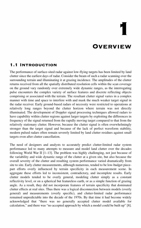
1Overview

1.1 IntroductionThe performance of surface-sited radar against low-flying targets has been limited by landclutter since the earliest days of radar. Consider the beam of such a radar scanning over thesurrounding terrain and illuminating it at grazing incidence. The amplitudes of the clutterreturns received from all the spatially distributed resolution cells within the scan coverageon the ground vary randomly over extremely wide dynamic ranges, as the interrogatingpulse encounters the complex variety of surface features and discrete reflecting objectscomprising or associated with the terrain. The resultant clutter signal varies in a complexmanner with time and space to interfere with and mask the much weaker target signal inthe radar receiver. Early ground-based radars of necessity were restricted to operations atrelatively long ranges beyond the clutter horizon where terrain was not directlyilluminated. The development of Doppler signal processing techniques allowed radars tohave capability within clutter regions against larger targets by exploiting the differences infrequency of the signal returned from the rapidly moving target compared to that from therelatively stationary clutter. However, because the clutter signal is often overwhelminglystronger than the target signal and because of the lack of perfect waveform stability,modern pulsed radars often remain severely limited by land clutter residues against smalltargets even after clutter cancellation.

The need of designers and analysts to accurately predict clutter-limited radar systemperformance led to many attempts to measure and model land clutter over the decadesfollowing World War II [1–13]. The problem was highly challenging, not just because ofthe variability and wide dynamic range of the clutter at a given site, but also because theoverall severity of the clutter and resulting system performance varied dramatically fromsite to site. Early clutter measurements, although numerous, tended to be low-budget piece-part efforts overly influenced by terrain specificity in each measurement scene. Inaggregate these efforts led to inconsistent, contradictory, and incomplete results. Earlyclutter models tended to be overly general, modeling clutter simply as a constantreflectivity level, or on a spherical but featureless earth, or as a simple function of grazingangle. As a result, they did not incorporate features of terrain specificity that dominatedclutter effects at real sites. Thus there was a logical disconnection between models (overlygeneral) and measurements (overly specific), and clutter-limited radar performanceremained unpredictable into the decade of the 1970s. By that time it had become widelyacknowledged that “there was no generally accepted clutter model available forcalculation,” and there was “no accepted approach by which a model could be built up” [8].

2 Overview

The middle and late 1970s also saw an emerging era of low-observable technology inaircraft design and consequent new demands on air defense capabilities in which liabilitiesimposed by the lack of predictability of clutter-limited surface radar performance weremuch heightened. As a result, a significant new activity was established at LincolnLaboratory in 1978 to advance the scientific understandings of air defense. An importantinitial element of this activity was the requirement to develop an accurate full-scale cluttersimulation capability that would breach the previous impasse. The goal was to make cluttermodeling a proper engineering endeavor typified by quantitative comparison of theory withmeasurement, and so allow confident prediction of clutter-limited performance of ground-sited radar.

It was believed on the basis of the historical evidence that a successful approach wouldhave to be strongly empirical. To this end, a major new program of land cluttermeasurements was initiated at Lincoln Laboratory [14–18]. To solve the land cluttermodeling problem, it was understood that the new measurements program would have tosubstantially raise the ante in terms of level of effort and new approaches compared withthose undertaken in the past. Underlying the key aspect of variability in the low-angleclutter phenomenon was the obvious fact that landscape itself was essentially infinitelyvariable—every clutter measurement scenario was different. Rather than seek the general inany individual measurement, underlying trends among aggregates of similar measurementswould be sought.

In ensuing years, a large volume of coherent multifrequency land clutter measurement datawas acquired (using dedicated new measurement instrumentation) from many sites widelydistributed geographically over the North American continent [14]. A new site-specificapproach was adopted in model development, based on the use of digitized terrain elevationdata (DTED) to distinguish between visible and masked regions to the radar, whichrepresented an important advance over earlier featureless or sandpaper-earth (i.e.,statistically rough) constructs [15]. Extensive analysis of the new clutter measurementsdatabase led to a progression of increasingly accurate statistical clutter models forspecifying the clutter in visible regions of clutter occurrence. A key requirement in thedevelopment of the statistical models was that only parametric trends directly observable inthe measurement data would be employed; any postulated dependencies that could not bedemonstrated to be statistically significant were discarded. As a result, a number of earlierinsights into low-angle clutter phenomenology were often understood in a new light andemployed in a different manner or at a different scale so as to reconcile with what wasactually observed in the data. In addition, significant new advances in understanding low-angle clutter occurred that, when incorporated properly with the modified earlier insights,led to a unified statistical approach for modeling low-angle clutter in which all importanttrends observable in the data were reproducible.

An empirically-based statistical clutter modeling capability now exists at LincolnLaboratory. Clutter-limited performance of surface-sited radar in benign or difficultenvironments is routinely and accurately predicted. Time histories of the signal-to-clutterratios existing in particular radars as they work against particular targets at particular sitesare computed and closely compared to measurements. Systems computations involvingtens or hundreds of netted radars are performed in which the ground clutter1 at each site ispredicted separately and specifically. Little incentive remains at Lincoln Laboratory todevelop generic non-site-specific approaches to clutter modeling for the benefit of saving

Overview 3

computer time, because the results of generic models lack specific realism and, as a result,are difficult to validate.

This book provides a thorough summary and review of the results obtained in the cluttermeasurements and modeling program at Lincoln Laboratory over a 20-year period. Thebook covers (1) prediction of clutter strength (Weibull statistical model2), (2) clutterspreading in Doppler (exponential model), and (3) given the strength and spreading ofclutter, the extent to which various techniques of clutter cancellation (e.g., simple delay-line cancellation vs coherent signal processing) can reduce the effects of clutter on targetdetection performance.

1.2 Historical ReviewAlthough most surface-sited radars partially suppress land clutter interference fromsurrounding terrain to provide some capability in cluttered spatial regions, the design ofclutter cancellers requires knowledge of the statistical properties of the clutter, and theclutter residues remaining after cancellation can still strongly limit radar performance (seeChapter 6, Sections 6.4.4 and 6.5). Because of this importance of land clutter to theoperations of surface radar, there were very many early attempts [1–9] to measure andcharacterize the phenomenon and bring it into analytic predictability. A literature review ofthe subject of low-angle land clutter as the Lincoln Laboratory clutter measurementprogram commenced found over 100 different preceding measurement programs and over300 different reports and journal articles on the subject. There exist many excellent sourcesof review [19–25] of these early efforts and preceding literature. These reviews withoutexception agree on the difficulty of generally characterizing low-angle land clutter.

The difficulty arises largely because of the complexity and variability of land-surface formand the elements of land cover that exist at a scale of radar wavelength (typically, from afew meters to a few centimeters or less) over the hundreds or thousands of squarekilometers of composite terrain that are usually under radar coverage at a typical radarsite. As a result, the earlier efforts [1–9] to understand low-angle land clutter revealed thatit was a highly non-Gaussian (i.e., non-noise-like), multifaceted, relatively intractable,statistical random process of which the most salient attribute was variability. Thevariability existed at whatever level the phenomenon was observed—pulse-to-pulse, cell-to-cell, or site-to-site.

Other important attributes of the low-angle clutter phenomenon included: patchiness inspatial occurrence [3–5]; lack of homogeneity and domination by point-like or spatiallydiscrete sources within spatial patches [6–8]; and extremely widely-skewed distributions ofclutter amplitudes over spatial patches often covering six orders of magnitude or more [1,2, 4, 9]. Early efforts to capture these attributes and dependencies in simple clutter models

1. This book uses the terms “land clutter” and “ground clutter” interchangeably to refer to the same phenome-non. The adjective “land” is more global in reach and distinguishes land clutter from other, generically dif-ferent types of clutter such as sea clutter or weather clutter. The adjective “ground” is often used when the subject focus is only on ground clutter, and more localized circumstances need to be distinguished, for example, the differences in ground clutter from one site to another, or from one area or type of ground to another.

2. Weibull statistics are used as approximations only—not rigorous fits—to measured clutter spatial ampli-tude distributions. See Chapter 2, Section 2.4.1.1; Chapter 5, Section 5.2.1 and Appendix 5.A.

4 Overview

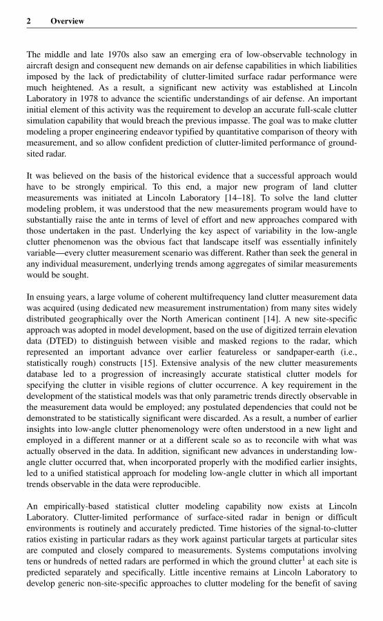
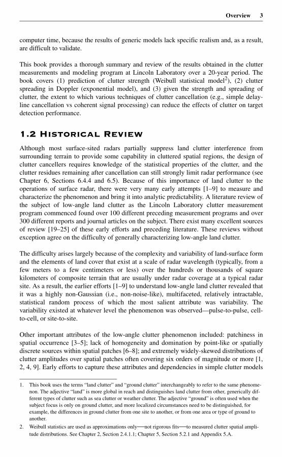
based only on range or illumination angle to the clutter cell were largely unsuccessful inbeing able to predict radar system performance. Figure 1.1 shows a measured plan-position-indicator (PPI) clutter map that illustrates to 24-km range at a western prairie sitethe spatial complexity and variability of low-angle land clutter. The fact that the clutterdoes not occur uniformly but is spatially patchy over the region of surveillance is evident inthis measurement, as is the granularity or discrete-like nature of the clutter such that it oftenoccurs in spatially isolated cells over regions where it does occur.

Although the earlier efforts and preceding literature did not lead to a satisfactory cluttermodel, they did in total gradually develop a number of useful insights into the complexityof the land clutter phenomenon. Section 1.2 provides a summary of what these insightswere, and the general approaches extant for attempting to bring the important observablesof low-angle clutter under predictive constructs, as the Lincoln Laboratory programcommenced.

1.2.1 Constant σ °

Initially, land clutter was conceptualized (unlike Figure 1.1) as arising from a spatiallyhomogeneous surface surrounding the radar site, of uniform roughness (like sandpaper) at a

Figure 1.1 Measured X-band ground clutter map; Orion, Alberta. Maximum range = 24 km. Cells with discernible clutter are shown white. A large clutter patch (i.e., macroregion) to the SSW is also shown outlined in white.

N

S

W E

Overview 5

scale of radar wavelength to account for clutter backscatter. The backscatter reflectivity ofthis surface was characterized as being a surface-area density function, that is, by a cluttercoefficient σ ° defined [20] to be the radar cross section (RCS) of the clutter signal returnedper unit terrain surface-area within the radar spatial resolution cell (see Section 2.3.1.1).This characterization implies a power-additive random process, in which each resolutioncell contains many elemental clutter scatterers of random amplitude and uniformlydistributed phase, such that the central limit theorem applies and the resultant clutter signalis Rayleigh-distributed in amplitude (like thermal noise).

As conceptualized in this simple manner, land clutter merely acts to uniformly raise thenoise level in the receiver, the higher noise level being directly determined by σ °. Aselected set of careful measurements of σ ° compiled in tables or handbooks for variouscombinations of terrain type (forest, farmland, etc.) and radar parameter (frequency,polarization) would allow radar system engineers to straightforwardly calculate signal-to-clutter ratios and estimate target detection statistics and other performance measures on thebasis of clutter statistics being like those of thermal noise, but stronger. Early radar systemengineering textbooks promoted this view. However, this approach led to frustration inpractice. Tabularization of σ ° into generally accepted, universal values proved elusive.Every measurement scenario seemed overly specific. Resulting matrices of σ ° numberscompiled from different investigators using different measurement instrumentationoperating at different landscape scales (e.g., long-range scanning surveillance radar vsshort-range small-spot-size experiments) and employing different data reductionprocedures were erratic and incomplete, with little evidence of consistency, general trend,or connective tissue.

1.2.2 Wide Clutter Amplitude Distributions

Clutter measurements that involved accumulating σ ° returns by scanning over a spatiallycontinuous neighborhood of generally similar terrain (i.e., clutter patch) found that theresulting clutter spatial amplitude distributions were of extreme, highly skewed shapes verymuch wider than Rayleigh [2, 4, 9]. Unlike the narrow fixed-shape Rayleigh distributionwith its tight mean-to-median ratio of only 1.6 dB, the measured broad distributions wereof highly variable shapes with mean-to-median ratios as high as 15 or even 30 dB.

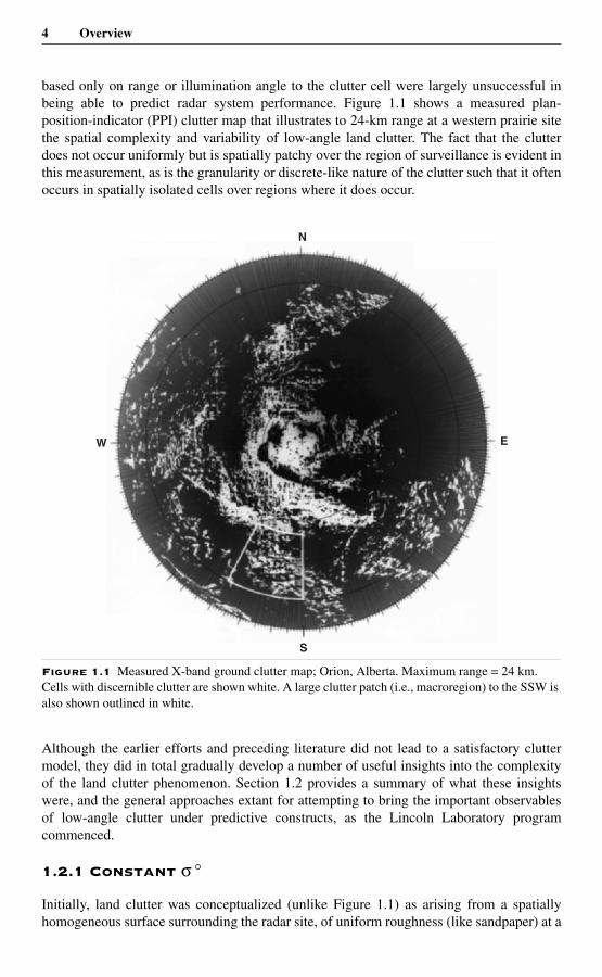
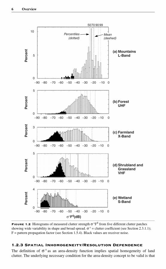
Figure 1.2 shows five measured clutter histograms from typical clutter patches such as thatshown in Figure 1.1, illustrating the wide variability in shape and broad spread that occursin such data. Thus in the important aspect of its amplitude distribution, low-angle landclutter was decidedly non-noise-like. This fact was at best only awkwardly reconcilablewith the constant-σ ° clutter model. The accompanying shapes of clutter distributions aswell as their mean σ ° levels required specification against radar and environmentalparameters, compounding the difficulties of compilation. As a result of both sea and landclutter measured distributions being wider than Rayleigh, an extensive literature came intobeing that addressed radar detection statistics in non-Rayleigh clutter backgrounds of widespread typically characterizable as lognormal, Weibull, or K-distributed [26–31]. However,the need continued for a single-point constant-σ ° clutter model to provide an averageindication of signal-to-clutter ratio which left the user with the nebulous question of whatsingle value of σ ° (e.g., mean, median, mode, etc.) to use to best characterize the wideunderlying distributions. Some investigators used the mean, others used the median, and itwas not always clear what was being used since it did not make much difference underRayleigh statistics and the question of underlying distribution was not always raised.

6 Overview

1.2.3 Spatial Inhomogeneity/Resolution DependenceThe definition of σ ° as an area-density function implies spatial homogeneity of landclutter. The underlying necessary condition for the area-density concept to be valid is that

Figure 1.2 Histograms of measured clutter strength σ °F4 from five different clutter patches showing wide variability in shape and broad spread. σ ° = clutter coefficient (see Section 2.3.1.1); F = pattern propagation factor (see Section 1.5.4). Black values are receiver noise.

0

0

0

0

0

4

3

5

5

5

10

σ°F4(dB)

(a) Mountains L-Band

Percentiles(dotted)

−90 −80 −70 −60 −50 −40 −30

5070 9099

−20 −10 0

(b) Forest UHF

−90 −80 −70 −60 −50 −40 −30 −20 −10 0

Per

cen

tP

erce

nt

(c) Farmland X-Band

−90 −80 −70 −60 −50 −40 −30 −20 −10 0

Per

cen

t

(d) Shrubland and Grassland VHF

−90 −80 −70 −60 −50 −40 −30 −20 −10 0

Per

cen

t

(e) Wetland S-Band

−90 −80 −70 −60 −50 −40 −30 −20 −10 0

Per

cen

t

Mean(dashed)

Overview 7

the mean value of σ ° be independent of the particular cell size or resolution utilized in agiven clutter spatial field.3 As mentioned, it was additionally presumed that much thesame invariant value of σ ° (tight Rayleigh variations) would exist among the individualspatial samples of σ ° independent of cell size. Early low-resolution radars showed landclutter generally surrounding the site and extending in range to the clutter horizon in anapproximately area-extensive manner. Measurements at higher resolution with narrowerbeams and shorter pulses showed that clutter was not present everywhere as from afeatureless sandpaper surface, but that resolved clutter typically occurred in patches orspatial regions of strong returns separated by regions of low returns near or at the radarnoise floor [4]—see Figure 1.1. Thus, clutter was highly non-noise-like not only in itsnon-Rayleigh amplitude statistics, but also in its lack of spatial homogeneity. High-resolution radars took advantage of the spatial non-homogeneity of clutter by providingsome operational capability known as interclutter visibility in relatively clear regionsbetween clutter patches [23].

Within clutter patches, clutter is not uniformly distributed. The individual spatial samplesof σ °, as opposed to their mean, depend strongly upon resolution cell size. Thus the shapesof the broad amplitude distributions of σ ° are highly dependent on resolution—increasingresolution results in less averaging within cells, more cell-to-cell variability, and increasingspread in values of σ °. In contrast, the fixed shape of a Rayleigh distribution describingsimple homogeneous clutter is invariant with resolution. Significant early work wasconducted into establishing necessary and sufficient conditions (e.g., number of scatterersand their relative amplitudes) in order for Rayleigh/Ricean statistics to prevail in temporalvariations from individual cells, but the associated idea of how cell size affects shapes ofspatial amplitude distributions from many individual cells was less a subject ofinvestigation.

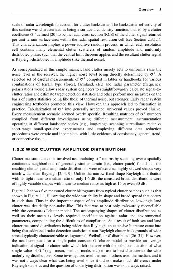
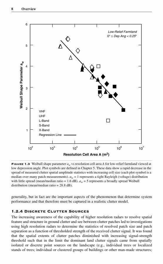
One early study got so far as to document an observed trend of increasing spread in clutterspatial amplitude distributions with increasing radar resolution [8], but this fundamentallyimportant observation into the nature of low-angle clutter4 was not generally followed upon or worked into empirical clutter models. Figure 1.3 shows how the Weibull shapeparameter aw (see Section 2.4.1.1), which controls the extent of spread in histograms suchas those of Figure 1.2, varies strongly with radar spatial resolution in low-relief farmlandviewed at low depression angle. These and many other such results for various terrain typesand viewing angles are presented and explained in Chapter 5.

These two key attributes of low-angle clutter—patchiness and lack of uniformity in spatialextent (Figure 1.1), and extreme resolution-dependent cell-to-cell variability in clutteramplitudes within spatial patches of occurrence (Figures 1.2 and 1.3)—do not constituteextraneous complexity to be avoided in formulating simple clutter models aimed at

3. By “clutter spatial field” is meant a region of [land surface] space characterized by a physical property [clut-ter strength] having a determinable value at every point [resolution cell] in the region; see American Heri-tage Dictionary of the English Language, 3rd ed. This book uses the phrase “clutter spatial field” or “clutter field” as so defined to bring to mind when it is a spatially-distributed ensemble of backscattering clutter res-olution cells that is of primary interest. The word “clutter” by itself can be vague (e.g., clutter signal vs clut-ter source; spatial vs temporal vs Doppler distribution), so that its use alone can bring different images to mind for different readers. Use of the phrase “clutter field” in this book does not refer to the strength of the propagating electromagnetic wave constituting the clutter return signal.

4. That is, the effect of resolution on the spatial as opposed to the temporal statistics of clutter.

8 Overview

generality, but in fact are the important aspects of the phenomenon that determine systemperformance and that therefore must be captured in a realistic clutter model.

1.2.4 Discrete Clutter SourcesThe increasing awareness of the capability of higher resolution radars to resolve spatialfeature and structure in ground clutter and see between clutter patches led to investigationsusing high resolution radars to determine the statistics of resolved patch size and patchseparation as a function of thresholded strength of the received clutter signal. It was foundthat the spatial extents of clutter patches diminished with increasing signal-strengththreshold such that in the limit the dominant land clutter signals came from spatiallyisolated or discrete point sources on the landscape (e.g., individual trees or localizedstands of trees; individual or clustered groups of buildings or other man-made structures;

Figure 1.3 Weibull shape parameter aw vs resolution cell area A for low-relief farmland viewed at low depression angle. Plot symbols are defined in Chapter 5. These data show a rapid decrease in the spread of measured clutter spatial amplitude statistics with increasing cell size (each plot symbol is a median over many patch measurements). aw = 1 represents a tight Rayleigh (voltage) distribution with little spread (mean/median ratio = 1.6 dB). aw = 5 represents a broadly spread Weibull distribution (mean/median ratio = 28.8 dB).

6

5

4

3

2

1

102 103 104 105 106 107

Resolution Cell Area A (m2)

Wei

bu

ll S

hap

e P

aram

eter

aw

VHF

UHF

L-Band

S-Band

X-Band

Regression Line

Low-Relief Farmland0° ≤ Dep Ang < 0.25°

Overview 9

utility poles and towers; local heights of land, hilltops, hummocks, river bluffs, and rockfaces) [6, 7]. This discrete or granular nature of the strongest clutter sources in low-angleclutter became relatively widely recognized—this granularity is quite evident in Figure1.1. It became typical for clutter models to consist of two components: a spatially-extensive background component modeled in terms of an area-density clutter coefficientσ °, and a discrete component modeled in terms of radar cross section (RCS) as being theappropriate measure for a point source of clutter isolated in its resolution cell and forwhich the strength of the RCS return is independent of the size of the cell encompassing it.The RCS levels of the discretes were specified by spatial incidence or density (so manyper square km), with the incidence diminishing as the specified level of discrete RCSincreased. Note that in such a representation for the discrete clutter component, althoughthe strength of the RCS return from a single discrete source is independent of the spatialresolution of the observing radar, the probability of a cell capturing zero vs one vs morethan one discrete does depend on resolution (i.e., discrete clutter is also affected by cellsize). It was usual in such two-component clutter models for the extended background σ °component to be developed more elaborately than the discrete RCS component, the latterusually being added in as an adjunct overlay to what was regarded as the main area-extensive phenomenon.

Although the two-component clutter model seemed conceptually simple and satisfactory asan idealized concept to deal with first-level observations, attempting to sort out measureddata following this approach was not so simple. The wide measured spatial amplitudedistributions of clutter were continuous in clutter strength over many (typically, as many assix or eight) orders of magnitude and did not separate nicely into what could be recognizedas a high-end cluster of strong discretes and a weaker bell-curve background. That is, inmeasured clutter data, there is no way of telling whether any given return is from a spatiallydiscrete or distributed clutter source [25]. Additional complication arises due to radarspatial resolution diminishing linearly with range (i.e., cross-range resolution is determinedby azimuth beamwidth) so that discretes of a given spatial density might be isolated at shortrange but not at longer ranges. The reality is that, at lower signal-strength thresholds,spatial cells capture more than one discrete and cell area affects returned clutter strength.This difficulty in the two-component model of how to transition in measured data andhence in modeling specification between extended σ ° and discrete RCS has been discussedvery little in the literature. These matters are discussed more extensively in Chapter 4,Section 4.5.

1.2.5 Illumination AngleTo many investigators, a land clutter model is basically just a characteristic of σ ° vsillumination angle in the vertical plane of incidence. The empirical relationship σ ° = γ sinψ where ψ is grazing angle (i.e., the angle between the terrain surface and the radar line-of-sight; see Figure 2.15 in Chapter 2) and γ is a constant dependent on terrain type and radarfrequency has come to be accepted as generally representative over a wide range of higher,airborne-like angles [24]. However, at the low angles of ground-based radar, typically withψ < 1° or 2°, it was not clear how to proceed. One relatively widely-held school ofthought5 was that at such low angles in typically-occurring low-relief terrain, grazing

5. The phrase “school of thought” rather than “opinion” is used here to indicate a point-of-view held by a group [more than one investigator] and to which some effort [as opposed to a preliminary idea] along the line indi-cated took place.

10 Overview

angle was a rather nebulous concept, neither readily definable [e.g., at what scale shouldsuch a definition be attempted, that of radar wavelength (cm) or that of landform variation(km)?] nor necessarily very directly related to the clutter strengths arising fromdiscontinuous or discrete sources of vertical discontinuity dominating the low-anglebackscatter and principally associated with land cover. From this point-of-view, the radarwave was more like a horizontally-propagating surface wave than one impinging at anangle from above, and it made more sense to separate the clutter by gross terrain type(mountains vs plains, forest vs farmland) than by fine distinctions in what were all veryoblique angles of incidence.

Another widely held school-of-thought was to extend the constant-γ model to the low-angle regime by adding a low-angle correction term to prevent σ ° from becomingvanishingly small at grazing incidence (as ψ → 0°). Little appropriate measurement data(for example, from in situ surveillance radars) was available upon which to base such acorrective term. Moreover, the idea of a corrective term tends to oversimplify the low-angleregime. At higher angles, the assumption behind a constant-γ model is of Rayleighstatistics; at low angles, it was known that the shapes of clutter amplitude distributions werebroader and modelable as Weibull or lognormal, but following through with informationspecifying shape parameters continuously with angle for corrected constant-γ models atlow angles was generally not attempted.

The gradually increasing availability of digitized terrain elevation data (DTED) in the1970s and 1980s, typically at about 100 m horizontal sampling interval and 1 mquantization in elevation, quickly led to its use by the low-angle clutter modelingcommunity. The hope was that the DTED would carry the burden of terrain representationby allowing the earth’s surface to be modeled as a grid of small interconnected triangularDTED planes or facets joining the points of terrain elevation. Then clutter modeling couldproceed relatively straightforwardly in the low-angle regime, as a function of grazing angle(e.g., constant-γ or extended constant-γ) on inclined DTED facets. This approach tomodeling low-angle clutter won a wide following and continues to receive much attention.Note that it is usually advocated as a seemingly sensible but unproven postulate, and not onthe basis of successful reduction of actual measurement data via grazing angle on DTEDfacets. As applied on a cell-by-cell (or facet-by-facet) basis, such a model is usuallythought of as returning deterministic samples of σ °, thus avoiding the difficult problem ofspecifying statistical clutter spreads at low angles (although such a model can returnrandom draws from statistical distributions if the distributions are specified). Indeed, whenapplied deterministically, the cell-to-cell scintillations in the simulated clutter signal causedby variations in DTED facet inclinations appear to mimic scintillation in measured cluttersignals. However, this simple deterministic approach to modeling generally does not resultin predicted low-angle clutter amplitude distributions matching measurement data.Predicted signal-to-clutter ratios and track errors recorded in radar tracking of low-altitudetargets across particular clutter spatial fields using such a model show little correlation withmeasured data.

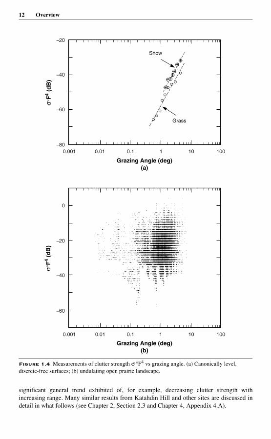
The root cause of this failure is that the bare-earth DTED-facet representation of terraindoes not carry sufficient information to alone account for radar backscatter; it lacksprecision and accuracy to define terrain slope at a scale of radar wavelength and providesno information on the discrete elements of land cover which dominate and causescintillation in the measurement data. This is illustrated by the results of Figure 1.4. At the

Overview 11

top, Figure 1.4(a) shows X-band measurements of clutter strength vs grazing angle in twoshort-range canonical situations where the clutter-producing surface was very level—on afrozen snow-covered lake and on an artificially level, mown-grass, ground-reflectingantenna range. In such situations, the computation of grazing angle is straightforward—it issimply equal to the depression angle below the horizontal at which the clutter cell isobserved at the radar antenna. In these two canonical or laboratory-like measurementsituations, a strong dependence of increasing clutter strength with increasing grazing angleis indicated.

Such results illustrate the thinking that lies behind the desire of many investigators to wantto establish a grazing-angle dependent clutter model. However, as shown in Figure 1.4(b),when grazing angle is computed to DTED facets used to model real terrain surfaces, littlecorrelation between clutter strength and grazing angle is seen in the results. Specifically,Figure 1.4(b) shows a scatter plot in which measured X-band clutter strength in each cell atthe undulating western prairie site of Beiseker, Alberta is paired with an estimate of grazingangle to the cell derived from a DTED model of the terrain at the site. As mentioned, thereasons that little or no correlation is seen in the results have to do with lack of accuracy inthe DTED and in the fact that the bare-earth DTED representation of the terrain surfacecontains no information on the spatially discrete land cover elements that usually dominatelow-angle clutter. Results such as those shown in Figure 1.4(b) are discussed at greaterlength in Chapter 2 (see Section 2.3.5). Such results illustrate why attempting deterministicprediction of low-angle clutter strength via grazing angle to DTED facets has been an over-simplified micro-approach that fails.

1.2.6 Range DependenceReturn now to the first school of thought mentioned in the preceding discussion concerningillumination angle, namely, that at grazing incidence in low-relief terrain, terrain slope andgrazing angle are neither very definable nor of basic consequence in low angle clutter.Within this school of thought, the central observable fact concerning clutter in a ground-based radar is its obvious dissipation with increasing range. Thus some early clutter modelsfor surface-sited radars were formulated from this point of view. Rather than model theclutter at microscale, such models treated the earth as a large featureless sphere, uniformlymicrorough to provide backscattering, but without specific large-scale terrain feature. Suchan earth does not provide spatial patchiness; rather it is uniformly illuminated everywhereto the horizon, and clutter strength is diminished with increasing range via propagationlosses over the spherical earth. This appears to be a simple general macroscale approach forproviding a range-dependent clutter model for surface-sited radar.

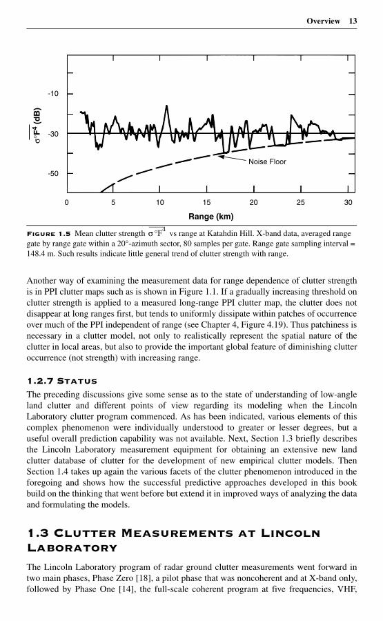
However, like the microscale grazing angle model, the macroscale range-dependent modeldoes not conform to the measurement data. These data show that what actually diminisheswith increasing range at real sites is the occurrence of the clutter—with increasing range,visible clutter-producing terrain regions become smaller, fewer, and farther between, until,beyond some maximum range, no more terrain is visible (see Chapter 4, Figure 4.10).Further, the measurement data show that clutter strength does not generally diminish withincreasing range, either within visible patches or from patch to patch. To illustrate this,Figure 1.5 shows mean clutter strength vs range in a 20o azimuth sector at Katahdin Hill,Massachusetts, looking out 30 km over hilly forested terrain. The data in this figurescintillate from gate to gate and occasionally drop to the noise floor where visibility toterrain is lost, but the average level stays at ~ –30 dB over the full extent in range with no

12 Overview

significant general trend exhibited of, for example, decreasing clutter strength withincreasing range. Many similar results from Katahdin Hill and other sites are discussed indetail in what follows (see Chapter 2, Section 2.3 and Chapter 4, Appendix 4.A).

Figure 1.4 Measurements of clutter strength σ °F4 vs grazing angle. (a) Canonically level, discrete-free surfaces; (b) undulating open prairie landscape.

–80

–60

–40

–20

0.001 0.01 0.1 1 10 100

Grass

Snow

Grazing Angle (deg)(a)

σ°F

4 (d

B)

–60

–40

–20

0

0.001 0.01 0.1 1 10 100

Grazing Angle (deg)(b)

σ°F

4 (d

B)

Overview 13

Another way of examining the measurement data for range dependence of clutter strengthis in PPI clutter maps such as is shown in Figure 1.1. If a gradually increasing threshold onclutter strength is applied to a measured long-range PPI clutter map, the clutter does notdisappear at long ranges first, but tends to uniformly dissipate within patches of occurrenceover much of the PPI independent of range (see Chapter 4, Figure 4.19). Thus patchiness isnecessary in a clutter model, not only to realistically represent the spatial nature of theclutter in local areas, but also to provide the important global feature of diminishing clutteroccurrence (not strength) with increasing range.

1.2.7 StatusThe preceding discussions give some sense as to the state of understanding of low-angleland clutter and different points of view regarding its modeling when the LincolnLaboratory clutter program commenced. As has been indicated, various elements of thiscomplex phenomenon were individually understood to greater or lesser degrees, but auseful overall prediction capability was not available. Next, Section 1.3 briefly describesthe Lincoln Laboratory measurement equipment for obtaining an extensive new landclutter database of clutter for the development of new empirical clutter models. ThenSection 1.4 takes up again the various facets of the clutter phenomenon introduced in theforegoing and shows how the successful predictive approaches developed in this bookbuild on the thinking that went before but extend it in improved ways of analyzing the dataand formulating the models.

1.3 Clutter Measurements at Lincoln LaboratoryThe Lincoln Laboratory program of radar ground clutter measurements went forward intwo main phases, Phase Zero [18], a pilot phase that was noncoherent and at X-band only,followed by Phase One [14], the full-scale coherent program at five frequencies, VHF,

Figure 1.5 Mean clutter strength vs range at Katahdin Hill. X-band data, averaged range gate by range gate within a 20°-azimuth sector, 80 samples per gate. Range gate sampling interval = 148.4 m. Such results indicate little general trend of clutter strength with range.

Range (km)

Noise Floor

0

-50

-30

-10

5 10 15 20 25 30

σ°F

4 (d

B)

σ °F4

14 Overview

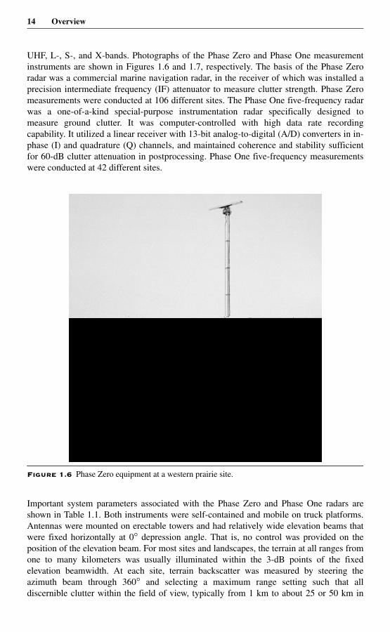
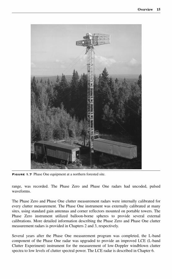
UHF, L-, S-, and X-bands. Photographs of the Phase Zero and Phase One measurementinstruments are shown in Figures 1.6 and 1.7, respectively. The basis of the Phase Zeroradar was a commercial marine navigation radar, in the receiver of which was installed aprecision intermediate frequency (IF) attenuator to measure clutter strength. Phase Zeromeasurements were conducted at 106 different sites. The Phase One five-frequency radarwas a one-of-a-kind special-purpose instrumentation radar specifically designed tomeasure ground clutter. It was computer-controlled with high data rate recordingcapability. It utilized a linear receiver with 13-bit analog-to-digital (A/D) converters in in-phase (I) and quadrature (Q) channels, and maintained coherence and stability sufficientfor 60-dB clutter attenuation in postprocessing. Phase One five-frequency measurementswere conducted at 42 different sites.

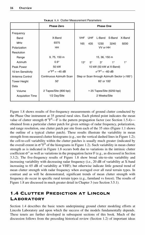
Important system parameters associated with the Phase Zero and Phase One radars areshown in Table 1.1. Both instruments were self-contained and mobile on truck platforms.Antennas were mounted on erectable towers and had relatively wide elevation beams thatwere fixed horizontally at 0° depression angle. That is, no control was provided on theposition of the elevation beam. For most sites and landscapes, the terrain at all ranges fromone to many kilometers was usually illuminated within the 3-dB points of the fixedelevation beamwidth. At each site, terrain backscatter was measured by steering theazimuth beam through 360° and selecting a maximum range setting such that alldiscernible clutter within the field of view, typically from 1 km to about 25 or 50 km in

Figure 1.6 Phase Zero equipment at a western prairie site.

Overview 15

range, was recorded. The Phase Zero and Phase One radars had uncoded, pulsedwaveforms.

The Phase Zero and Phase One clutter measurement radars were internally calibrated forevery clutter measurement. The Phase One instrument was externally calibrated at manysites, using standard gain antennas and corner reflectors mounted on portable towers. ThePhase Zero instrument utilized balloon-borne spheres to provide several externalcalibrations. More detailed information describing the Phase Zero and Phase One cluttermeasurement radars is provided in Chapters 2 and 3, respectively.

Several years after the Phase One measurement program was completed, the L-bandcomponent of the Phase One radar was upgraded to provide an improved LCE (L-bandClutter Experiment) instrument for the measurement of low-Doppler windblown clutterspectra to low levels of clutter spectral power. The LCE radar is described in Chapter 6.

Figure 1.7 Phase One equipment at a northern forested site.

16 Overview

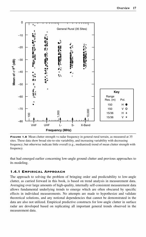
Figure 1.8 shows results of five-frequency measurements of ground clutter conducted bythe Phase One instrument at 35 general rural sites. Each plotted point indicates the meanvalue of clutter strength σ °F4—F is the pattern propagation factor (see Section 1.5.4)—obtained from a particular clutter patch for given settings of radar frequency, polarization,and range resolution, one clutter patch per site from each of the 35 sites (Figure 1.1 showsthe outline of a typical clutter patch). These results illustrate the variability in meanstrength from measured clutter histograms (e.g., see the vertical dashed lines in Figure 1.2);the cell-to-cell variability within the clutter patches is usually much greater (indicated bythe overall extent in σ°F4 of the histograms in Figure 1.2). Such variability in mean clutterstrength as is indicated in Figure 1.8 occurs both due to variations in the intrinsic cluttercoefficient σ° as well as variations in the propagation factor F (e.g., as discussed in Section3.3.2). The five-frequency results of Figure 1.8 show broad site-to-site variability andincreasing variability with decreasing radar frequency (i.e., 20 dB of variability at X-bandincreasing to 65 dB of variability at VHF); but otherwise indicate little general trend ofmean clutter strength with radar frequency when averaged over all rural terrain types. Incontrast and as will be demonstrated, significant trends of mean clutter strength withfrequency do occur in specific rural terrain types (e.g., farmland vs forest). The results ofFigure 1.8 are discussed in much greater detail in Chapter 3 (see Section 3.5.1).

1.4 Clutter Prediction at Lincoln LaboratorySection 1.4 describes the basic tenets underpinning ground clutter modeling efforts atLincoln Laboratory and upon which the success of the models fundamentally depends.These tenets are further developed in subsequent sections of this book. Much of thediscussion follows from the preceding historical review (Section 1.2) of important ideas

Table 1.1 Clutter Measurement Parameters

Phase Zero

Frequency

Band

MHz

Polarization

Resolution

Range

Azimuth

Peak Power

10 km Sensitivity

Antenna Control

Tower Height

Data

Volume

Acquisition Time

X-Band

9375

HH

9, 75, 150 m

0.9°

50 kW

�°F4 = –45 dB

Continuous Azimuth Scan

50'

2 Tapes/Site (800 bpi)

1/2 Day/Site

Phase One

VHF UHF L-Band S-Band X-Band

VV or HH

15, 36, 150 m

10 kW (50 kW at X-Band)

�°F4 = –60 dB

Step or Scan through Azimuth Sector (<185°)

60' or 100'

~ 25 Tapes/Site (6250 bpi)

2 Weeks/Site

~

13° 5° 3° 1° 1°

165 435 1230 3240 9200

Overview 17

that had emerged earlier concerning low-angle ground clutter and previous approaches toits modeling.

1.4.1 Empirical ApproachThe approach to solving the problem of bringing order and predictability to low-angleclutter, as carried forward in this book, is based on trend analysis in measurement data.Averaging over large amounts of high-quality, internally self-consistent measurement dataallows fundamental underlying trends to emerge which are often obscured by specificeffects in individual measurements. No attempts are made to hypothesize and validatetheoretical solutions, and any notional dependencies that cannot be demonstrated in thedata are also not utilized. Empirical predictive constructs for low-angle clutter in surfaceradar are developed based on replicating all important general trends observed in themeasurement data.

Figure 1.8 Mean clutter strength vs radar frequency in general rural terrain, as measured at 35 sites. These data show broad site-to-site variability, and increasing variability with decreasing frequency; but otherwise indicate little overall (e.g., medianized) trend of mean clutter strength with frequency.

0

–10

–20

–30

–40

–50

–60

–70

–80VHF

RangeRes. (m) Pol.

150

150

15/36

15/36

H

V

H

V

UHF L- S- X-Band

General Rural (35 Sites)10

0

1,00

0

10,0

00

Mea

n o

f σ°

F4 (

dB

)

Frequency (MHz)

Key

18 Overview

1.4.2 Deterministic PatchinessAs stated previously, the most salient characteristic of ground clutter in a surface radar isvariability. One important way that this variability manifests itself is patchiness in spatialoccurrence (see Figure 1.1). Clutter does not exist everywhere, and its on-again, off-againbehavior is what fundamentally determines system performance at any given site. Themain approach of this book presumes the use of DTED to deterministically approximatethe site-specific spatial patterns of terrain visibility and hence clutter occurrence at eachsite of interest. Following this approach, answers about the degree to which clutter limitssystem performance are obtainable one site at a time. Clutter varies dramatically from siteto site, and the extent to which clutter limits radar performance only has deterministicmeaning on a site-specific basis. Some effort (coordinated with studies at LincolnLaboratory) has been made elsewhere [32] to include mathematically-derived stochasticpatchiness within a general non-site-specific clutter modeling framework, but in suchefforts the statistics of patchiness, dependent upon terrain type, are themselves obtainedfrom processing in DTED for the terrain type of interest. A site-specific deterministically-patchy model allows quantitative comparison between prediction and measurement ofgiven clutter patches at given sites; more general stochastically-patchy or non-patchymodels cannot be validated in this direct manner.

1.4.3 Statistical ClutterAlthough the visible regions of occurrences of ground clutter (i.e., the macroscale clutterspatial occupancy map—see Figure 1.1) are predicted deterministically using DTED, theclutter amplitudes that occur distributed over such regions are a statistical phenomenon.The information content in DTED is suitable for defining kilometer-sized macroregions ofterrain visibility, but this information content—in currently available or any foreseeabledatabase of digitized terrain elevations and/or terrain descriptive information—isinsufficient to deterministically predict clutter amplitudes in individual spatial cells. Thusthis book characterizes land clutter strength (as opposed to its spatial occupancy map) as astatistical random process and determines predictive parametric trends in the parameterscharacterizing the statistical clutter amplitude distributions.

1.4.4 One-Component σ ° ModelThe difficulty in two-component clutter models6 of how to transition in measured data andmodeling specification between extended σ ° and discrete RCS was previously broughtinto consideration in Section 1.2.4. Consider again the key role that spatial resolutionplays in low-angle ground clutter (see Section 1.2.3). The shapes of clutter spatialamplitude distributions are highly dependent on resolution over their whole extents (notjust their strong-side tails). This results from the fact that at grazing incidence much of thediscernible clutter (not just the strongest returns) is discrete-like. This key fact has beenrelatively unrecognized in the clutter literature, although occasional past remarks may befound that begin to approach the idea. For example, Krason and Randig [3] based theinterpretation of their measurements of forest clutter on what appeared to them to be afundamental “transition from diffuse scattering at large angles to specular scattering at thevery shallow angles.” Recall that surface clutter as originally conceptualized—wherein allcells, whether large or small, contain large numbers of small scatterers—providesamplitude distributions with unvarying tight Rayleigh shapes and no dependence of shape

6. “Two-component clutter model” is defined in Section 1.2.4.

Overview 19

on resolution. In contrast, what the radar is actually collecting at low angles is a broadcontinuum of spiky returns from discretes over a wide range of amplitudes, such that thereare usually a number of discretes in each cell. This number is small enough that changingcell size strongly affects the statistics of the results.

Recognition of this fact allows the complete spatial field of low-angle land clutter fromweakest to strongest cells to be understood and predicted in a unified manner using an area-extensive σ ° formulation. The approach properly deals with cells containing a number ofrelatively weak, randomly-phased discretes as a power-additive density function in thestatistical aggregate of many such cells. However, the approach also properly treatsoccasional cells containing strong isolated discretes, despite the fact that representingisolated discretes with a density function may at first seem inappropriate. For such a cell, ahigh-resolution radar will contribute a strong σ ° into a wide amplitude distribution, and alow-resolution radar will contribute a weaker σ ° into a narrower amplitude distribution.Prediction of clutter RCS from these distributions will result in the same RCS for the largediscrete in both cells (large σ ° times small cell area equals smaller σ ° times larger cellarea).

Thus a statistical σ ° model implementing the fundamental property of spread in amplitudedistribution vs resolution can capture and recreate the observed spatial granularity andpoint-like nature of clutter fields at low angles of observation, without recourse to anadditional RCS component that is difficult to implement realistically. The reasoning behindwhy the density function σ ° is the proper way to model clutter even when dominated bydiscrete sources is considerably expanded upon in Chapter 4, Section 4.5. The cluttermodeling statistics provided in this book follow this approach (but see Appendix 4.D).

1.4.5 Depression AngleReturn now to the preceding discussion (Section 1.2.5) of historical perceptions on whetherillumination angle might be important in affecting low-angle clutter strength, and if so, howto implement it in a model. Another position on how to use illumination angle to helpcharacterize low-angle clutter, intermediate between that of not using angle at all(following the first approach described in Section 1.2.5) and that based on fine-scalespecification of local terrain slopes in DTED (following the subsequent approach describedin Section 1.2.5), exists and was utilized in the early literature by Linell [1] to successfullyreduce measurement data from a ground-sited radar working over ranges up to 12 km.7

Although terrain slopes may not be very definable or directly relatable to clutter strengthsat grazing incidence (as under the first approach described in Section 1.2.5), thisintermediate approach brings a more macroscopic measure of angle to bear on the problem,namely the depression angle at which larger patches of relatively uniform terrain areviewed below the local horizontal at the radar antenna. The use of DTED to definedepression angle as a macroparameter in this manner is appropriate to the informationcontent and accuracy of the DTED, in contrast to the use of DTED to define grazing angleas a microparameter associated with individual cells. That is, depression angle dependsonly on terrain elevations and not their rates of change and hence is a slowly varying

7. That is, at more realistic ranges for surface radar than the several tens or hundreds of meters of many mea-

surements of σ ° vs grazing angle reported in the literature and performed, for example, with radars mounted on portable “cherry-pickers” for the purpose of measuring backscatter from small areas of homoge-neous ground and for the most part at higher angles [40].

20 Overview

quantity over clutter patches; whereas grazing angle depends also on rates of change ofelevation (i.e., the derivative) and hence is a rapidly varying quantity much moresusceptible to inaccuracies and error tolerances in DTED. Linell’s results [1] showed thatlevels and shapes of clutter amplitude distributions measured from such macropatches wereextremely sensitive to the differences in depression angle (e.g., 0.7°, 1.25°, 5°) at whichthey were obtained. These data became widely referenced [21, 24, 26], but did not directlylead to clutter models. An important distinction is that such data did not directly provide asimple continuous angle characteristic (like constant-γ), but instead showed howcomplete clutter amplitude distributions vary in steps or intervals of depression angleregime.

Similar effects with depression angle, as first seen much earlier by Linell, both on themean levels and shapes of clutter amplitude distributions over large spatial macroregionsof low-angle clutter occurrence, constitute a highly pervasive and important parametricinfluence observed throughout the Phase Zero and Phase One measurements. Figure 1.9shows these strong effects of depression angle on levels and shapes of clutter amplitudedistributions. The curves of Figure 1.9 are plotted from the Phase Zero X-band data inTable 2.4 of Chapter 2; they were first presented in this manner by Skolnik [19]. It isevident in these results that mean and median clutter strengths rise rapidly with increasingdepression angle, and that spreads in clutter amplitude distributions as given by either themean/median ratio (as shown in the lower part of Figure 1.9) or by the Weibull shapeparameter aw rapidly decrease with increasing angle (the upper part of Figure 1.9 plots theinverse of aw against depression angle). The results shown in Figure 1.9 are described ingreater detail in Chapter 2.

Although Linell’s results reporting the sensitivity of shape parameter to angle wererelatively widely referenced, the corresponding similar sensitivity of shape parameter toradar spatial resolution was less widely recognized, as of course were the consequentinterdependent effects of angle and resolution together on shape. These importantinterdependent effects of both depression angle (Figure 1.9) and radar resolution (Figure1.3) on the shapes of low-angle clutter amplitude distributions are key elements in theclutter modeling information provided in this book.

1.4.6 Decoupling of Radar Frequency and ResolutionStatistical low-angle clutter amplitude distributions are fundamentally characterized by amean absolute level, and by the shape or degree of spread (broad or narrow) about the meanlevel. Results in this book show that the mean level of the distribution depends strongly onradar frequency, depending on terrain type (see Figure 3.38);8 and that the shape of thedistribution depends strongly on radar spatial resolution (as has been discussed, see Figure1.3). In addition, both the mean level and the shape depend upon depression angle (seeFigure 1.9). However, analyses of the clutter measurement data have uncovered animportant further fact, fundamental to the development of the modeling information in thisbook. This further fact is the decoupling of the effects of radar frequency and resolution on

8. To be clear what is meant, this book shows that there exists little or no general dependence of land clutter strength with radar carrier frequency, VHF to X-band, where by “general” is meant averaging across all spe-cific terrain types; but that for specific terrain types the frequency dependence of clutter can be strong, rang-ing from varying directly with carrier frequency (i.e., strongly increasing with frequency) in open low-relief terrain to varying inversely with carrier frequency (i.e., strongly decreasing with frequency) in forested high-relief terrain (see Chapters 3 and 5).

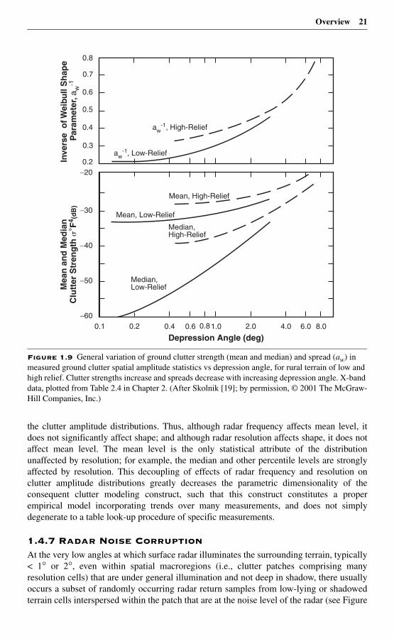
Overview 21

the clutter amplitude distributions. Thus, although radar frequency affects mean level, itdoes not significantly affect shape; and although radar resolution affects shape, it does notaffect mean level. The mean level is the only statistical attribute of the distributionunaffected by resolution; for example, the median and other percentile levels are stronglyaffected by resolution. This decoupling of effects of radar frequency and resolution onclutter amplitude distributions greatly decreases the parametric dimensionality of theconsequent clutter modeling construct, such that this construct constitutes a properempirical model incorporating trends over many measurements, and does not simplydegenerate to a table look-up procedure of specific measurements.

1.4.7 Radar Noise CorruptionAt the very low angles at which surface radar illuminates the surrounding terrain, typically< 1° or 2°, even within spatial macroregions (i.e., clutter patches comprising manyresolution cells) that are under general illumination and not deep in shadow, there usuallyoccurs a subset of randomly occurring radar return samples from low-lying or shadowedterrain cells interspersed within the patch that are at the noise level of the radar (see Figure

Figure 1.9 General variation of ground clutter strength (mean and median) and spread (aw) in measured ground clutter spatial amplitude statistics vs depression angle, for rural terrain of low and high relief. Clutter strengths increase and spreads decrease with increasing depression angle. X-band data, plotted from Table 2.4 in Chapter 2. (After Skolnik [19]; by permission, © 2001 The McGraw-Hill Companies, Inc.)

Inve

rse

of W

eibu

ll S

hap

e P

aram

eter

, aw

-1M

ean

an

d M

edia

nC

lutt

er S

tren

gth

�° F

4 (dB

)

Depression Angle (deg)

0.8

0.7

0.6

0.5

0.4

0.3

0.2

−30

−20

−40

−50

−600.1 0.2 0.4 0.6 0.81.0 2.0 4.0 6.0 8.0

aw-1, Low-Relief

aw-1, High-Relief

Mean, High-Relief

Mean, Low-Relief

Median,High-Relief

Median,Low-Relief

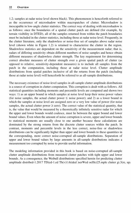
22 Overview

1.2; samples at radar noise level shown black). This phenomenon is henceforth referred toas the occurrence of microshadow within macropatches of clutter. Microshadow isinescapable in low-angle clutter statistics. The correct way of dealing with microshadow isas follows: once the boundaries of a spatial clutter patch are defined (for example, byterrain visibility in DTED), all of the samples returned from within the patch boundariesmust be included in the clutter statistics, including those at radar noise level. Frequently, inthe clutter literature, only the shadowless or noise-free set of samples above radar noiselevel (shown white in Figure 1.2) is retained to characterize the clutter in the region.Shadowless statistics are dependent on the sensitivity of the measurement radar; that is,radars of differing sensitivity obtain different numbers of noise samples and hence obtaindifferent measures of shadowless clutter strength. The key requirement for determiningcorrect absolute measures of clutter strength over a given spatial patch of clutter (asopposed to relative, sensitivity-dependent measures) is to include all samples from thepatch in the computation, including those at radar noise level. Clutter amplitudedistributions from spatial patches inclusive of all the returns from the patch (includingthose at radar noise level) will henceforth be referred to as all-sample distributions.

The necessary existence of noise-level samples in all-sample clutter amplitude distributionsis a source of corruption in clutter computation. This corruption is dealt with as follows. Allstatistical quantities including moments and percentile levels are computed and shown twoways: 1) as an upper bound in which samples at noise level keep their noise power values(for noise samples, the actual clutter power ≤ noise power); and 2) as a lower bound inwhich the samples at noise level are assigned zero or a very low value of power (for noisesamples, the actual clutter power ≥ zero). The correct value of the statistical quantity, thatis, the value that would be measured by a theoretically infinitely sensitive radar for whichthe upper and lower bounds would coalesce, must lie between the upper bound and lowerbound values. Even when the amount of noise corruption is severe, upper and lower boundsto statistical moments are usually close to one another because these calculations aredominated by the strong returns from the discrete clutter sources within the patch. Incontrast, moments and percentile levels in the less correct, noise-free or shadowlessdistributions can be significantly higher than upper and lower bounds to these quantities inthe corresponding, more correct noise-corrupted all-sample distributions. Separation ofupper and lower bound values by large amounts in all-sample distributions indicates ameasurement too corrupted by noise to provide useful information.

The modeling information provided in this book is based on noise-corrupted all-sampleclutter amplitude distributions from measured clutter patches with tight upper and lowerbounds. As a consequence, the Weibull distributions specified herein for predicting clutter

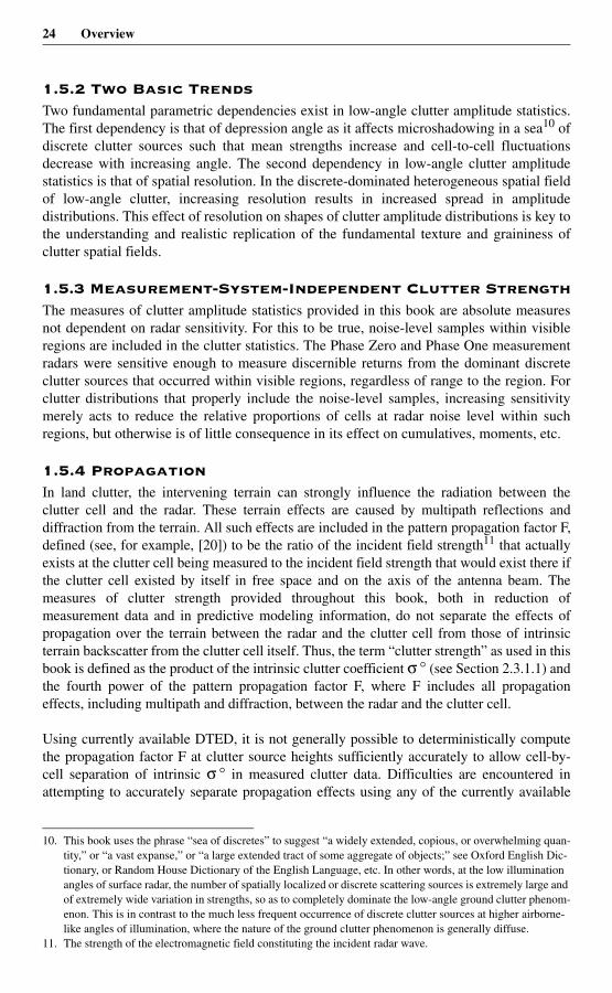
24 Overview

1.5.2 Two Basic TrendsTwo fundamental parametric dependencies exist in low-angle clutter amplitude statistics.The first dependency is that of depression angle as it affects microshadowing in a sea10 ofdiscrete clutter sources such that mean strengths increase and cell-to-cell fluctuationsdecrease with increasing angle. The second dependency in low-angle clutter amplitudestatistics is that of spatial resolution. In the discrete-dominated heterogeneous spatial fieldof low-angle clutter, increasing resolution results in increased spread in amplitudedistributions. This effect of resolution on shapes of clutter amplitude distributions is key tothe understanding and realistic replication of the fundamental texture and graininess ofclutter spatial fields.

1.5.3 Measurement-System-Independent Clutter StrengthThe measures of clutter amplitude statistics provided in this book are absolute measuresnot dependent on radar sensitivity. For this to be true, noise-level samples within visibleregions are included in the clutter statistics. The Phase Zero and Phase One measurementradars were sensitive enough to measure discernible returns from the dominant discreteclutter sources that occurred within visible regions, regardless of range to the region. Forclutter distributions that properly include the noise-level samples, increasing sensitivitymerely acts to reduce the relative proportions of cells at radar noise level within suchregions, but otherwise is of little consequence in its effect on cumulatives, moments, etc.

1.5.4 PropagationIn land clutter, the intervening terrain can strongly influence the radiation between theclutter cell and the radar. These terrain effects are caused by multipath reflections anddiffraction from the terrain. All such effects are included in the pattern propagation factor F,defined (see, for example, [20]) to be the ratio of the incident field strength11 that actuallyexists at the clutter cell being measured to the incident field strength that would exist there ifthe clutter cell existed by itself in free space and on the axis of the antenna beam. Themeasures of clutter strength provided throughout this book, both in reduction ofmeasurement data and in predictive modeling information, do not separate the effects ofpropagation over the terrain between the radar and the clutter cell from those of intrinsicterrain backscatter from the clutter cell itself. Thus, the term “clutter strength” as used in thisbook is defined as the product of the intrinsic clutter coefficient σ ° (see Section 2.3.1.1) andthe fourth power of the pattern propagation factor F, where F includes all propagationeffects, including multipath and diffraction, between the radar and the clutter cell.

Using currently available DTED, it is not generally possible to deterministically computethe propagation factor F at clutter source heights sufficiently accurately to allow cell-by-cell separation of intrinsic σ ° in measured clutter data. Difficulties are encountered inattempting to accurately separate propagation effects using any of the currently available

10. This book uses the phrase “sea of discretes” to suggest “a widely extended, copious, or overwhelming quan-tity,” or “a vast expanse,” or “a large extended tract of some aggregate of objects;” see Oxford English Dic-tionary, or Random House Dictionary of the English Language, etc. In other words, at the low illumination angles of surface radar, the number of spatially localized or discrete scattering sources is extremely large and of extremely wide variation in strengths, so as to completely dominate the low-angle ground clutter phenom-enon. This is in contrast to the much less frequent occurrence of discrete clutter sources at higher airborne-like angles of illumination, where the nature of the ground clutter phenomenon is generally diffuse.

11. The strength of the electromagnetic field constituting the incident radar wave.

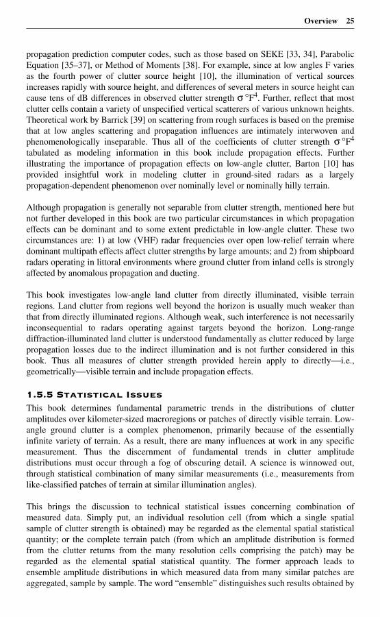
Overview 25

propagation prediction computer codes, such as those based on SEKE [33, 34], ParabolicEquation [35–37], or Method of Moments [38]. For example, since at low angles F variesas the fourth power of clutter source height [10], the illumination of vertical sourcesincreases rapidly with source height, and differences of several meters in source height cancause tens of dB differences in observed clutter strength σ °F4. Further, reflect that mostclutter cells contain a variety of unspecified vertical scatterers of various unknown heights.Theoretical work by Barrick [39] on scattering from rough surfaces is based on the premisethat at low angles scattering and propagation influences are intimately interwoven andphenomenologically inseparable. Thus all of the coefficients of clutter strength σ °F4

tabulated as modeling information in this book include propagation effects. Furtherillustrating the importance of propagation effects on low-angle clutter, Barton [10] hasprovided insightful work in modeling clutter in ground-sited radars as a largelypropagation-dependent phenomenon over nominally level or nominally hilly terrain.

Although propagation is generally not separable from clutter strength, mentioned here butnot further developed in this book are two particular circumstances in which propagationeffects can be dominant and to some extent predictable in low-angle clutter. These twocircumstances are: 1) at low (VHF) radar frequencies over open low-relief terrain wheredominant multipath effects affect clutter strengths by large amounts; and 2) from shipboardradars operating in littoral environments where ground clutter from inland cells is stronglyaffected by anomalous propagation and ducting.

This book investigates low-angle land clutter from directly illuminated, visible terrainregions. Land clutter from regions well beyond the horizon is usually much weaker thanthat from directly illuminated regions. Although weak, such interference is not necessarilyinconsequential to radars operating against targets beyond the horizon. Long-rangediffraction-illuminated land clutter is understood fundamentally as clutter reduced by largepropagation losses due to the indirect illumination and is not further considered in thisbook. Thus all measures of clutter strength provided herein apply to directly—i.e.,geometrically—visible terrain and include propagation effects.

1.5.5 Statistical IssuesThis book determines fundamental parametric trends in the distributions of clutteramplitudes over kilometer-sized macroregions or patches of directly visible terrain. Low-angle ground clutter is a complex phenomenon, primarily because of the essentiallyinfinite variety of terrain. As a result, there are many influences at work in any specificmeasurement. Thus the discernment of fundamental trends in clutter amplitudedistributions must occur through a fog of obscuring detail. A science is winnowed out,through statistical combination of many similar measurements (i.e., measurements fromlike-classified patches of terrain at similar illumination angles).

This brings the discussion to technical statistical issues concerning combination ofmeasured data. Simply put, an individual resolution cell (from which a single spatialsample of clutter strength is obtained) may be regarded as the elemental spatial statisticalquantity; or the complete terrain patch (from which an amplitude distribution is formedfrom the clutter returns from the many resolution cells comprising the patch) may beregarded as the elemental spatial statistical quantity. The former approach leads toensemble amplitude distributions in which measured data from many similar patches areaggregated, sample by sample. The word “ensemble” distinguishes such results obtained by

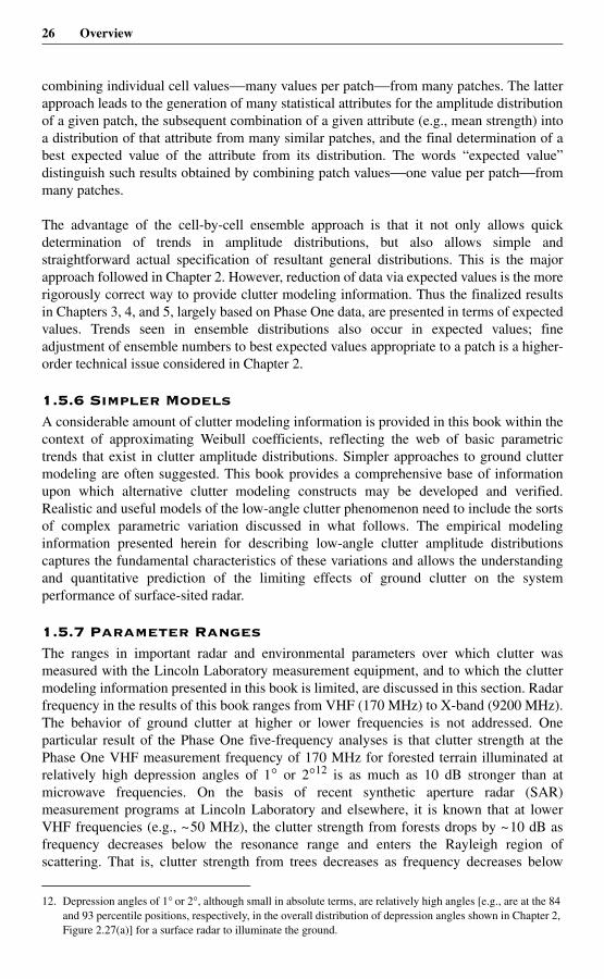
26 Overview

combining individual cell values—many values per patch—from many patches. The latterapproach leads to the generation of many statistical attributes for the amplitude distributionof a given patch, the subsequent combination of a given attribute (e.g., mean strength) intoa distribution of that attribute from many similar patches, and the final determination of abest expected value of the attribute from its distribution. The words “expected value”distinguish such results obtained by combining patch values—one value per patch—frommany patches.

The advantage of the cell-by-cell ensemble approach is that it not only allows quickdetermination of trends in amplitude distributions, but also allows simple andstraightforward actual specification of resultant general distributions. This is the majorapproach followed in Chapter 2. However, reduction of data via expected values is the morerigorously correct way to provide clutter modeling information. Thus the finalized resultsin Chapters 3, 4, and 5, largely based on Phase One data, are presented in terms of expectedvalues. Trends seen in ensemble distributions also occur in expected values; fineadjustment of ensemble numbers to best expected values appropriate to a patch is a higher-order technical issue considered in Chapter 2.

1.5.6 Simpler ModelsA considerable amount of clutter modeling information is provided in this book within thecontext of approximating Weibull coefficients, reflecting the web of basic parametrictrends that exist in clutter amplitude distributions. Simpler approaches to ground cluttermodeling are often suggested. This book provides a comprehensive base of informationupon which alternative clutter modeling constructs may be developed and verified.Realistic and useful models of the low-angle clutter phenomenon need to include the sortsof complex parametric variation discussed in what follows. The empirical modelinginformation presented herein for describing low-angle clutter amplitude distributionscaptures the fundamental characteristics of these variations and allows the understandingand quantitative prediction of the limiting effects of ground clutter on the systemperformance of surface-sited radar.

1.5.7 Parameter RangesThe ranges in important radar and environmental parameters over which clutter wasmeasured with the Lincoln Laboratory measurement equipment, and to which the cluttermodeling information presented in this book is limited, are discussed in this section. Radarfrequency in the results of this book ranges from VHF (170 MHz) to X-band (9200 MHz).The behavior of ground clutter at higher or lower frequencies is not addressed. Oneparticular result of the Phase One five-frequency analyses is that clutter strength at thePhase One VHF measurement frequency of 170 MHz for forested terrain illuminated atrelatively high depression angles of 1° or 2°12 is as much as 10 dB stronger than atmicrowave frequencies. On the basis of recent synthetic aperture radar (SAR)measurement programs at Lincoln Laboratory and elsewhere, it is known that at lowerVHF frequencies (e.g., ~50 MHz), the clutter strength from forests drops by ~10 dB asfrequency decreases below the resonance range and enters the Rayleigh region ofscattering. That is, clutter strength from trees decreases as frequency decreases below

12. Depression angles of 1° or 2°, although small in absolute terms, are relatively high angles [e.g., are at the 84 and 93 percentile positions, respectively, in the overall distribution of depression angles shown in Chapter 2, Figure 2.27(a)] for a surface radar to illuminate the ground.

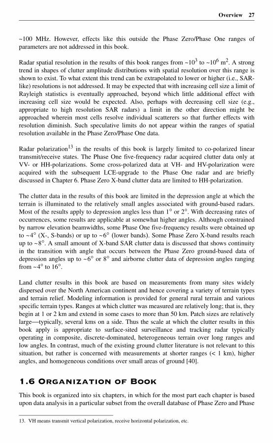
Overview 27

~100 MHz. However, effects like this outside the Phase Zero/Phase One ranges ofparameters are not addressed in this book.

Radar spatial resolution in the results of this book ranges from ~103 to ~106 m2. A strongtrend in shapes of clutter amplitude distributions with spatial resolution over this range isshown to exist. To what extent this trend can be extrapolated to lower or higher (i.e., SAR-like) resolutions is not addressed. It may be expected that with increasing cell size a limit ofRayleigh statistics is eventually approached, beyond which little additional effect withincreasing cell size would be expected. Also, perhaps with decreasing cell size (e.g.,appropriate to high resolution SAR radars) a limit in the other direction might beapproached wherein most cells resolve individual scatterers so that further effects withresolution diminish. Such speculative limits do not appear within the ranges of spatialresolution available in the Phase Zero/Phase One data.

Radar polarization13 in the results of this book is largely limited to co-polarized lineartransmit/receive states. The Phase One five-frequency radar acquired clutter data only atVV- or HH-polarizations. Some cross-polarized data at VH- and HV-polarization wereacquired with the subsequent LCE-upgrade to the Phase One radar and are brieflydiscussed in Chapter 6. Phase Zero X-band clutter data are limited to HH-polarization.

The clutter data in the results of this book are limited in the depression angle at which theterrain is illuminated to the relatively small angles associated with ground-based radars.Most of the results apply to depression angles less than 1° or 2°. With decreasing rates ofoccurrences, some results are applicable at somewhat higher angles. Although constrainedby narrow elevation beamwidths, some Phase One five-frequency results were obtained upto ~4° (X-, S-bands) or up to ~6° (lower bands). Some Phase Zero X-band results reachup to ~8°. A small amount of X-band SAR clutter data is discussed that shows continuityin the transition with angle that occurs between the Phase Zero ground-based data ofdepression angles up to ~6° or 8° and airborne clutter data of depression angles rangingfrom ~4° to 16°.

Land clutter results in this book are based on measurements from many sites widelydispersed over the North American continent and hence covering a variety of terrain typesand terrain relief. Modeling information is provided for general rural terrain and variousspecific terrain types. Ranges at which clutter was measured are relatively long; that is, theybegin at 1 or 2 km and extend in some cases to more than 50 km. Patch sizes are relativelylarge—typically, several kms on a side. Thus the scale at which the clutter results in thisbook apply is appropriate to surface-sited surveillance and tracking radar typicallyoperating in composite, discrete-dominated, heterogeneous terrain over long ranges andlow angles. In contrast, much of the existing ground clutter literature is not relevant to thissituation, but rather is concerned with measurements at shorter ranges (< 1 km), higherangles, and homogeneous conditions over small areas of ground [40].

1.6 Organization of BookThis book is organized into six chapters, in which for the most part each chapter is basedupon data analysis in a particular subset from the overall database of Phase Zero and Phase

13. VH means transmit vertical polarization, receive horizontal polarization, etc.

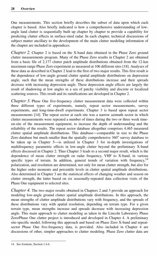
28 Overview

One measurements. This section briefly describes the subset of data upon which eachchapter is based. Also briefly indicated is how a comprehensive understanding of low-angle land clutter is sequentially built up chapter by chapter to provide a capability forpredicting clutter effects in surface-sited radar. In each chapter, technical discussions ofsubject matter ancillary to the development of the main clutter modeling information ofthe chapter are included in appendices.

Chapter 2. Chapter 2 is based on the X-band data obtained in the Phase Zero groundclutter measurements program. Many of the Phase Zero results in Chapter 2 are obtainedfrom a basic file of 2,177 clutter patch amplitude distributions obtained from the 12-kmmaximum range Phase Zero experiment as measured at 106 different sites [18]. Analyses ofthese data as described in Chapter 2 lead to the first of two major results. This first result isthe dependence of low-angle ground clutter spatial amplitude distributions on depressionangle, such that the mean strengths of these distributions increase and their spreadsdecrease with increasing depression angle. These depression angle effects are largely theresult of shadowing at low angles in a sea of patchy visibility and discrete or localizedscattering sources. This result and its ramifications are developed in Chapter 2.

Chapter 3. Phase One five-frequency clutter measurement data were collected withinthree different types of experiments, namely, repeat sector measurements, surveyexperiments, and long-time-dwell experiments. Chapter 3 is based upon repeat sectormeasurements [14]. The repeat sector at each site was a narrow azimuth sector in whichclutter measurements were repeated a number of times during the two or three week time-on-site of the measurement equipment, to increase the depth of understanding and thereliability of the results. The repeat sector database altogether comprises 4,465 measuredclutter spatial amplitude distributions. This database—comparable in size to the PhaseZero database but much smaller than the spatially comprehensive 360° survey database tobe taken up in Chapter 5—is utilized in Chapter 3 for in-depth investigations ofmultifrequency parametric effects in low-angle clutter beyond the preliminary X-bandeffects discussed in Chapter 2. Thus Chapter 3 leads to a second major result, which is thedependence of mean clutter strength on radar frequency, VHF to X-band, in variousspecific types of terrain. In addition, general trends of variation with frequency,14

polarization, and resolution are determined, not only for mean clutter strength, but also forthe higher order moments and percentile levels in clutter spatial amplitude distributions.Also determined in Chapter 3 are the statistical effects of changing weather and season onclutter strength, the latter based on six seasonally-repeated data collection visits of thePhase One equipment to selected sites.

Chapter 4. The two major results obtained in Chapters 2 and 3 provide an approach formodeling low-angle ground clutter spatial amplitude distributions. In this approach, themean strengths of clutter amplitude distributions vary with frequency, and the spreads ofthese distributions vary with spatial resolution, depending on terrain type. For a giventerrain type, mean strengths increase and spreads decrease with increasing depressionangle. This main approach to clutter modeling as taken in the Lincoln Laboratory PhaseZero/Phase One clutter project is introduced and developed in Chapter 4. A preliminarysite-specific model, following this approach and based on Phase Zero X-band and repeat-sector Phase One five-frequency data, is provided. Also included in Chapter 4 arediscussions of other, simpler approaches to clutter modeling. Phase Zero clutter data are

14. See footnote, Section 1.4.6.

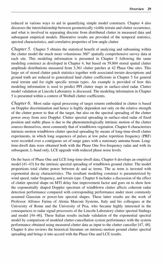
Overview 29

reduced in various ways to aid in quantifying simple model constructs. Chapter 4 alsodiscusses the interrelationship between geometrically visible terrain and clutter occurrence,and what is involved in separating discrete from distributed clutter in measured data andsubsequent empirical models. Illustrative results are provided of the temporal statistics,spectral characteristics, and correlative properties of low-angle clutter.

Chapter 5. Chapter 5 obtains the statistical benefit of analyzing and subsuming withinthe clutter model the much more voluminous 360° spatially comprehensive survey data ateach site. This modeling information is presented in Chapter 5 following the samemodeling construct as developed in Chapter 4, but based on 59,804 stored spatial clutteramplitude distributions measured from 3,361 clutter patches at 42 Phase One sites. Thislarge set of stored clutter patch statistics together with associated terrain descriptions andground truth are reduced to generalized land clutter coefficients in Chapter 5 for generalrural terrain and for eight specific terrain types. An example is provided of how thismodeling information is used to predict PPI clutter maps in surface-sited radar. Cluttermodel validation at Lincoln Laboratory is discussed. The modeling information in Chapter5 is presented within a context of Weibull clutter coefficients.

Chapter 6. Most radar signal processing of target returns embedded in clutter is basedon Doppler discrimination and hence is highly dependent not only on the relative strengthof the clutter power to that of the target, but also on the spectral spreading of the clutterpower away from zero Doppler. Clutter spectral spreading in surface-sited radar of fixedposition and stable phase is due to the phenomenologically intrinsic motion of the cluttersources themselves, most commonly that of windblown vegetation. Chapter 6 characterizesintrinsic-motion windblown clutter spectral spreading by means of long-time-dwell clutterexperiments, in which long sequences of pulses at low pulse repetition frequency (PRF)were recorded over a contiguous set of range gates with a stationary antenna beam. Long-time-dwell data were obtained both with the Phase One five-frequency radar and with itssubsequent, L-band only, LCE upgrade with reduced phase noise levels.

On the basis of Phase One and LCE long-time-dwell data, Chapter 6 develops an empiricalmodel [41–43] for the intrinsic spectral spreading of windblown ground clutter. The modelproportions total clutter power between dc and ac terms. The ac term is invested withexponential decay characteristics. The resultant modeling construct is parameterized bywind speed, radar frequency, and terrain type. Chapter 6 includes a discussion of the effectof clutter spectral shape on MTI delay line improvement factor and goes on to show howthe exponentially shaped Doppler spectrum of windblown clutter affects coherent radardetection performance compared with corresponding performance under more commonlyassumed Gaussian or power-law spectral shapes. These latter results are the work ofProfessor Alfonso Farina of Alenia Marconi Systems, Italy and his colleagues at theUniversity of Rome and the University of Pisa, who became highly interested in theconsequences to radar signal processors of the Lincoln Laboratory clutter spectral findingsand model [44–46]. These Italian results include validation of the exponential spectralmodel by comparison of modeled clutter-cancellation system performance with the systemperformance obtained using measured clutter data as input to the clutter canceller [47, 48].Chapter 6 also reviews the historical literature on intrinsic-motion ground clutter spectralspreading and brings it into accord with the Phase One and LCE results.

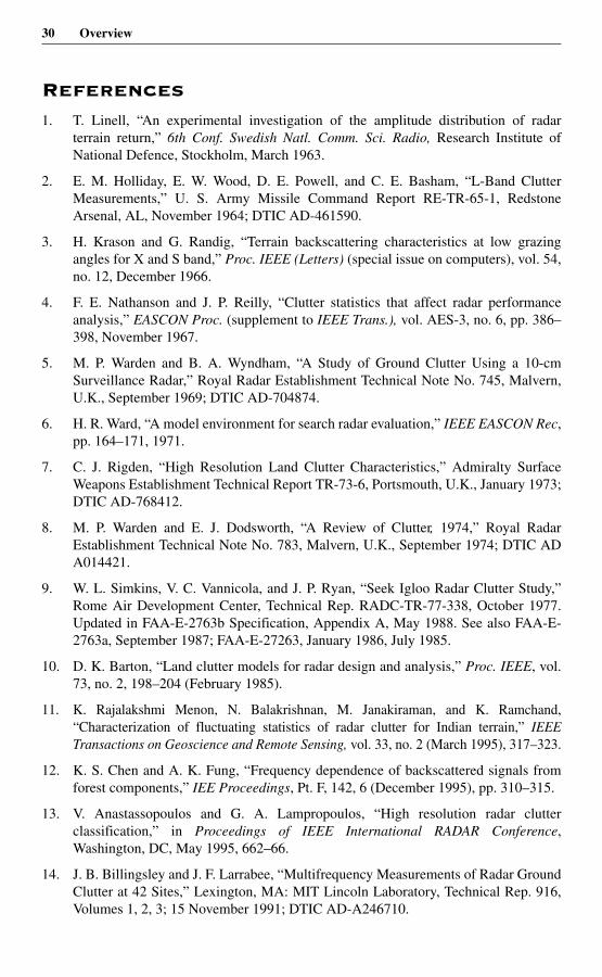
30 Overview

References1. T. Linell, “An experimental investigation of the amplitude distribution of radar

terrain return,” 6th Conf. Swedish Natl. Comm. Sci. Radio, Research Institute ofNational Defence, Stockholm, March 1963.

2. E. M. Holliday, E. W. Wood, D. E. Powell, and C. E. Basham, “L-Band ClutterMeasurements,” U. S. Army Missile Command Report RE-TR-65-1, RedstoneArsenal, AL, November 1964; DTIC AD-461590.

3. H. Krason and G. Randig, “Terrain backscattering characteristics at low grazingangles for X and S band,” Proc. IEEE (Letters) (special issue on computers), vol. 54,no. 12, December 1966.

4. F. E. Nathanson and J. P. Reilly, “Clutter statistics that affect radar performanceanalysis,” EASCON Proc. (supplement to IEEE Trans.), vol. AES-3, no. 6, pp. 386–398, November 1967.

5. M. P. Warden and B. A. Wyndham, “A Study of Ground Clutter Using a 10-cmSurveillance Radar,” Royal Radar Establishment Technical Note No. 745, Malvern,U.K., September 1969; DTIC AD-704874.

6. H. R. Ward, “A model environment for search radar evaluation,” IEEE EASCON Rec,pp. 164–171, 1971.

7. C. J. Rigden, “High Resolution Land Clutter Characteristics,” Admiralty SurfaceWeapons Establishment Technical Report TR-73-6, Portsmouth, U.K., January 1973;DTIC AD-768412.

8. M. P. Warden and E. J. Dodsworth, “A Review of Clutter, 1974,” Royal RadarEstablishment Technical Note No. 783, Malvern, U.K., September 1974; DTIC ADA014421.

9. W. L. Simkins, V. C. Vannicola, and J. P. Ryan, “Seek Igloo Radar Clutter Study,”Rome Air Development Center, Technical Rep. RADC-TR-77-338, October 1977.Updated in FAA-E-2763b Specification, Appendix A, May 1988. See also FAA-E-2763a, September 1987; FAA-E-27263, January 1986, July 1985.

10. D. K. Barton, “Land clutter models for radar design and analysis,” Proc. IEEE, vol.73, no. 2, 198–204 (February 1985).

11. K. Rajalakshmi Menon, N. Balakrishnan, M. Janakiraman, and K. Ramchand,“Characterization of fluctuating statistics of radar clutter for Indian terrain,” IEEETransactions on Geoscience and Remote Sensing, vol. 33, no. 2 (March 1995), 317–323.

12. K. S. Chen and A. K. Fung, “Frequency dependence of backscattered signals fromforest components,” IEE Proceedings, Pt. F, 142, 6 (December 1995), pp. 310–315.

13. V. Anastassopoulos and G. A. Lampropoulos, “High resolution radar clutterclassification,” in Proceedings of IEEE International RADAR Conference,Washington, DC, May 1995, 662–66.

14. J. B. Billingsley and J. F. Larrabee, “Multifrequency Measurements of Radar GroundClutter at 42 Sites,” Lexington, MA: MIT Lincoln Laboratory, Technical Rep. 916,Volumes 1, 2, 3; 15 November 1991; DTIC AD-A246710.

Overview 31

15. J. B. Billingsley, “Ground Clutter Measurements for Surface-Sited Radar,”Lexington, MA: MIT Lincoln Laboratory, Technical Rep. 786, Rev. 1, 1 February1993; DTIC AD-A262472.

16. J. B. Billingsley, “Radar ground clutter measurements and models, part 1: Spatialamplitude statistics,” AGARD Conf. Proc. Target and Clutter Scattering and TheirEffects on Military Radar Performance, Ottawa, AGARD-CP-501, 1991; DTIC AD-P006 373.

17. J. B. Billingsley, A. Farina, F. Gini, M. V. Greco, and L. Verrazzani, “Statisticalanalyses of measured radar ground clutter data,” IEEE Trans. AES, vol. 35, no. 2(April 1999).

18. J. B. Billingsley, “Low-Angle X-Band Radar Ground Clutter Spatial AmplitudeStatistics,” Lexington, MA: MIT Lincoln Laboratory, Technical Report 958, 2002.

19. M. I. Skolnik, Introduction to Radar Systems (3rd ed)., New York: McGraw-Hill, 2001.

20. L. V. Blake, Radar Range-Performance Analysis (2nd ed.), Silver Spring, MD:Monroe Publishing, 1991.

21. M. W. Long, Radar Reflectivity of Land and Sea (3rd ed.), Boston: Artech House,Inc., 2001.

22. C. Currie, “Clutter Characteristics and Effects,” in Principles of Modern Radar, J. L.Eaves and E. K. Reedy (Eds.), New York: Chapman & Hall, 1987.

23. D. K. Barton, Modern Radar System Analysis, Norwood, MA: Artech House, 1988.

24. F. E. Nathanson (with J. P. Reilly and M. N. Cohen), Radar Design Principles (2nded.), New York: McGraw-Hill, 1991.Reprinted, SciTech Publishing, Inc., 1999.

25. D. C. Schleher, MTI and Pulsed Doppler Radar, Norwood, MA: Artech House, 1991.

26. R. R. Boothe, “The Weibull Distribution Applied to the Ground Clutter BackscatterCoefficient,” U. S. Army Missile Command Rept. No. RE-TR-69-15, RedstoneArsenal, AL, June 1969; DTIC AD-691109.

27. M. Sekine and Y. Mao, Weibull Radar Clutter, London, U. K.: Peter Peregrinus Ltd.,1990.

28. E. Jakeman, “On the statistics of K-distributed noise,” J. Physics A; Math. Gen., vol.13, 31–48 (1980).

29. J. K. Jao, “Amplitude distribution of composite terrain radar clutter and the K-distribution,” IEEE Trans. Ant. Prop., vol. AP-32, no. 10, 1049–1062 (October 1984).

30. K. D. Ward, “Application of the K-distribution to radar clutter—A review,” Proc.Internat. Symp. on Noise and Clutter Rejection in Radars and Imaging Sensors, pp.15–21, IEICE, Tokyo (1989).

31. T. J. Nohara and S. Haykin, “Canadian East Coast radar trials and the K-distribution,” IEE Proceedings, Pt. F, 138, 2 (Apr. 1991), 80–88.

32. S. P. Tonkin and M. A. Wood, “Stochastic model of terrain effects upon theperformance of land-based radars,” AGARD Conference Proceedings on Target andClutter Scattering and Their Effects on Military Radar Performance, AGARD-CP-501, (1991).

32 Overview

33. S. Ayasli, “A computer model for low altitude radar propagation over irregularterrain,” IEEE Trans. Ant. Prop., vol. AP-34, no. 8, pp. 1013–1023 (August 1986).

34. M. P. Shatz and G. H. Polychronopoulos, “An algorithm for the evaluation of radarpropagation in the spherical earth diffraction region,” The Lincoln LaboratoryJournal, vol. 1, no. 2, 145–152 (Fall 1988).

35. G. D. Dockery and J. R. Kuttler, “An improved impedance boundary algorithm forFourier split-step solutions of the parabolic wave equation,” IEEE Trans. Ant. Prop.,44 (12), 1592–1599 (1996).

36. A. E. Barrios, “A terrain parabolic equation model for propagation in thetroposphere,” IEEE Trans. Ant. Prop., 42 (1), 90–98 (January 1994).

37. D. J. Donohue and J. R. Kuttler, “Modeling radar propagation over terrain,” JohnsHopkins APL Technical Digest, vol. 18, no. 2, 279–287, (April–June 1997).

38. J. T. Johnson, R. T. Shin, J. C. Eidson, L. Tsang, and J. A. Kong, “A method ofmoments model for VHF propagation,” IEEE Trans. Ant. Prop., 45 (1), 115–125(January 1997).

39. D.E. Barrick, “Grazing behavior of scatter and propagation above any roughsurface,” IEEE Trans. Ant. Prop., vol. 46, no. 1, pp. 73–83 (January 1998).

40. F. T. Ulaby and M. C. Dobson, Handbook of Radar Scattering Statistics for Terrain,Norwood, MA: Artech House, 1989.

41. J. B. Billingsley and J. F. Larrabee, “Measured Spectral Extent of L- and X-BandRadar Reflections from Windblown Trees,” Lexington, MA: MIT LincolnLaboratory, Project Rep. CMT-57, 6 February 1987; DTIC AD-A179942.

42. J. B. Billingsley, “Exponential Decay in Windblown Radar Ground Clutter DopplerSpectra: Multifrequency Measurements and Model,” Lexington, MA: MIT LincolnLaboratory, Technical Report 997, 29 July 1996; DTIC AD-A312399.

43. J. B. Billingsley, “Windblown radar ground clutter Doppler spectra: measurementsand model,” submitted to IEEE Trans. AES, accepted subject to minor revision,October 2000.

44. J. B. Billingsley, A. Farina, F. Gini, M. V. Greco, P. Lombardo, “Impact ofexperimentally measured Doppler spectrum of ground clutter on MTI and STAP,” inProceedings of IEE International Radar Conference (Radar ‘97), IEE Conf. Pub. No.449, pp. 290–294, Edinburgh, 14–16 October 1997.

45. P. Lombardo, M. V. Greco, F. Gini, A. Farina, and J. B. Billingsley, “Impact of clutterspectra on radar performance prediction,”IEEE Trans. AES, Vol. 37, no. 3, July 2001.

46. P. Lombardo and J. B. Billingsley, “A new model for the Doppler spectrum ofwindblown radar ground clutter,” in Proceedings of IEEE 1999 Radar Conference,Boston, MA: 20–22 April 1999.

47. M. V. Greco, F. Gini, A. Farina, and J. B. Billingsley, “Analysis of cluttercancellation in the presence of measured L-band radar ground clutter data,” inProceedings of IEEE International Radar Conference (Radar 2000), Alexandria,VA, May 8–12, 2000.

Overview 33

48. M. V. Greco, F. Gini, A. Farina, and J. B. Billingsley, “Validation of windblown radarground clutter spectral shape,” IEEE Trans. AES, vol. 37, no. 2, April 2001.

2Preliminary X-Band Clutter

Measurements

2.1 IntroductionChapter 2 provides general information describing the amplitude distributions of X-bandland clutter returns received from regions of visible ground, based on Phase Zeromeasurements at 106 sites. Subsequent chapters provide similar information at otherfrequencies. In presenting land clutter data and results, Chapter 2 attempts both to dojustice to describing a very complex phenomenon, and also to efficiently provide usefuland easily accessible modeling information. The result is a chapter that providesincreasing insight into the clutter phenomenon by cyclically building up an understandingof the many interacting influences affecting clutter amplitude statistics. As insights aredeveloped, they are accompanied with the presentation of modeling information thatgeneralizes such influences at various levels of fidelity.

2.1.1 Outline The major results of Chapter 2 are summarized within this section.

Basic Clutter Modeling Information. Chapter 2 provides basic ensemble modelinginformation describing X-band clutter amplitude distributions over macropatches of visibleterrain as a function of depression angle for three comprehensive terrain types—rural/low-relief, rural/high-relief, and urban. Chapter 2 goes on to explain, enlarge upon, and extendthe nature of low-angle clutter amplitude statistics as encoded within the basic modelinginformation.

Angle Characteristic. There traditionally has existed within the body of ground clutterliterature the idea that a clutter model could be a simple characteristic of clutter strength vsillumination angle. Such a model is provided in Chapter 2 as an expected-valuegeneralization of all the Phase Zero measurements. However, ground clutter is inherently astatistical phenomenon in which large statistical variation occurs. Thus this simple angle-characteristic model shows two characteristics of clutter strength, mean and median, vsangle. Together these characteristics demonstrate the important fact that clutter is statisticaland show not only clutter strength vs angle, but also specify the variability (i.e., mean-to-median ratio) of clutter strength at any given angle.

Worst-Case Situations. The basic X-band modeling information of Chapter 2 providesgeneral information. Chapter 2 also provides upper bounds on how strong ground cluttercan become in exceptional circumstances by comparing the amplitude distributions from

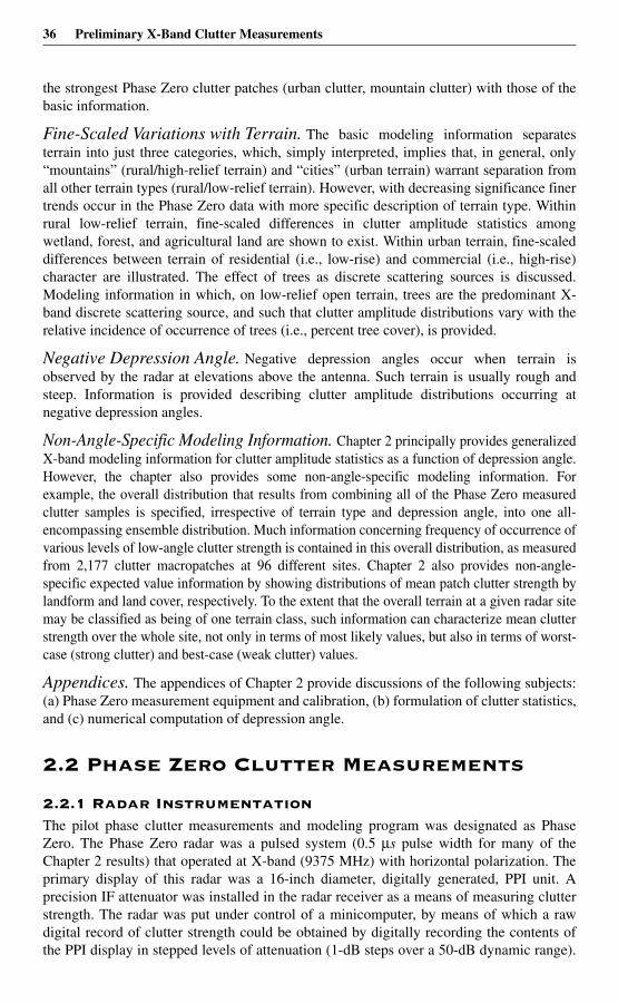
36 Preliminary X-Band Clutter Measurements

the strongest Phase Zero clutter patches (urban clutter, mountain clutter) with those of thebasic information.

Fine-Scaled Variations with Terrain. The basic modeling information separatesterrain into just three categories, which, simply interpreted, implies that, in general, only“mountains” (rural/high-relief terrain) and “cities” (urban terrain) warrant separation fromall other terrain types (rural/low-relief terrain). However, with decreasing significance finertrends occur in the Phase Zero data with more specific description of terrain type. Withinrural low-relief terrain, fine-scaled differences in clutter amplitude statistics amongwetland, forest, and agricultural land are shown to exist. Within urban terrain, fine-scaleddifferences between terrain of residential (i.e., low-rise) and commercial (i.e., high-rise)character are illustrated. The effect of trees as discrete scattering sources is discussed.Modeling information in which, on low-relief open terrain, trees are the predominant X-band discrete scattering source, and such that clutter amplitude distributions vary with therelative incidence of occurrence of trees (i.e., percent tree cover), is provided.

Negative Depression Angle. Negative depression angles occur when terrain isobserved by the radar at elevations above the antenna. Such terrain is usually rough andsteep. Information is provided describing clutter amplitude distributions occurring atnegative depression angles.

Non-Angle-Specific Modeling Information. Chapter 2 principally provides generalizedX-band modeling information for clutter amplitude statistics as a function of depression angle.However, the chapter also provides some non-angle-specific modeling information. Forexample, the overall distribution that results from combining all of the Phase Zero measuredclutter samples is specified, irrespective of terrain type and depression angle, into one all-encompassing ensemble distribution. Much information concerning frequency of occurrence ofvarious levels of low-angle clutter strength is contained in this overall distribution, as measuredfrom 2,177 clutter macropatches at 96 different sites. Chapter 2 also provides non-angle-specific expected value information by showing distributions of mean patch clutter strength bylandform and land cover, respectively. To the extent that the overall terrain at a given radar sitemay be classified as being of one terrain class, such information can characterize mean clutterstrength over the whole site, not only in terms of most likely values, but also in terms of worst-case (strong clutter) and best-case (weak clutter) values.

Appendices. The appendices of Chapter 2 provide discussions of the following subjects:(a) Phase Zero measurement equipment and calibration, (b) formulation of clutter statistics,and (c) numerical computation of depression angle.

2.2 Phase Zero Clutter Measurements

2.2.1 Radar Instrumentation The pilot phase clutter measurements and modeling program was designated as PhaseZero. The Phase Zero radar was a pulsed system (0.5 µs pulse width for many of theChapter 2 results) that operated at X-band (9375 MHz) with horizontal polarization. Theprimary display of this radar was a 16-inch diameter, digitally generated, PPI unit. Aprecision IF attenuator was installed in the radar receiver as a means of measuring clutterstrength. The radar was put under control of a minicomputer, by means of which a rawdigital record of clutter strength could be obtained by digitally recording the contents ofthe PPI display in stepped levels of attenuation (1-dB steps over a 50-dB dynamic range).

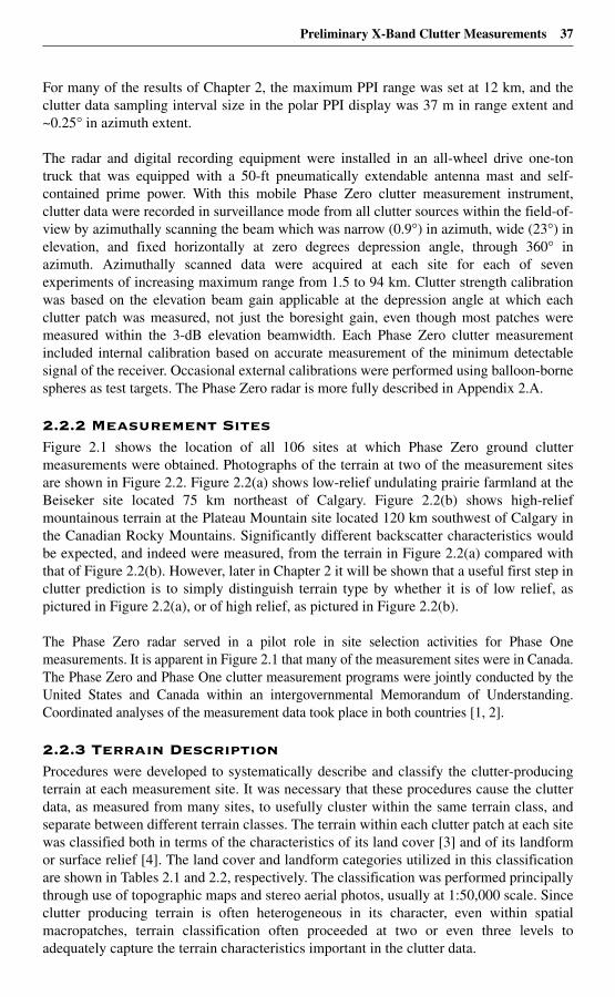
Preliminary X-Band Clutter Measurements 37

For many of the results of Chapter 2, the maximum PPI range was set at 12 km, and theclutter data sampling interval size in the polar PPI display was 37 m in range extent and~0.25° in azimuth extent.

The radar and digital recording equipment were installed in an all-wheel drive one-tontruck that was equipped with a 50-ft pneumatically extendable antenna mast and self-contained prime power. With this mobile Phase Zero clutter measurement instrument,clutter data were recorded in surveillance mode from all clutter sources within the field-of-view by azimuthally scanning the beam which was narrow (0.9°) in azimuth, wide (23°) inelevation, and fixed horizontally at zero degrees depression angle, through 360° inazimuth. Azimuthally scanned data were acquired at each site for each of sevenexperiments of increasing maximum range from 1.5 to 94 km. Clutter strength calibrationwas based on the elevation beam gain applicable at the depression angle at which eachclutter patch was measured, not just the boresight gain, even though most patches weremeasured within the 3-dB elevation beamwidth. Each Phase Zero clutter measurementincluded internal calibration based on accurate measurement of the minimum detectablesignal of the receiver. Occasional external calibrations were performed using balloon-bornespheres as test targets. The Phase Zero radar is more fully described in Appendix 2.A.

2.2.2 Measurement SitesFigure 2.1 shows the location of all 106 sites at which Phase Zero ground cluttermeasurements were obtained. Photographs of the terrain at two of the measurement sitesare shown in Figure 2.2. Figure 2.2(a) shows low-relief undulating prairie farmland at theBeiseker site located 75 km northeast of Calgary. Figure 2.2(b) shows high-reliefmountainous terrain at the Plateau Mountain site located 120 km southwest of Calgary inthe Canadian Rocky Mountains. Significantly different backscatter characteristics wouldbe expected, and indeed were measured, from the terrain in Figure 2.2(a) compared withthat of Figure 2.2(b). However, later in Chapter 2 it will be shown that a useful first step inclutter prediction is to simply distinguish terrain type by whether it is of low relief, aspictured in Figure 2.2(a), or of high relief, as pictured in Figure 2.2(b).

The Phase Zero radar served in a pilot role in site selection activities for Phase Onemeasurements. It is apparent in Figure 2.1 that many of the measurement sites were in Canada.The Phase Zero and Phase One clutter measurement programs were jointly conducted by theUnited States and Canada within an intergovernmental Memorandum of Understanding.Coordinated analyses of the measurement data took place in both countries [1, 2].

2.2.3 Terrain DescriptionProcedures were developed to systematically describe and classify the clutter-producingterrain at each measurement site. It was necessary that these procedures cause the clutterdata, as measured from many sites, to usefully cluster within the same terrain class, andseparate between different terrain classes. The terrain within each clutter patch at each sitewas classified both in terms of the characteristics of its land cover [3] and of its landformor surface relief [4]. The land cover and landform categories utilized in this classificationare shown in Tables 2.1 and 2.2, respectively. The classification was performed principallythrough use of topographic maps and stereo aerial photos, usually at 1:50,000 scale. Sinceclutter producing terrain is often heterogeneous in its character, even within spatialmacropatches, terrain classification often proceeded at two or even three levels toadequately capture the terrain characteristics important in the clutter data.

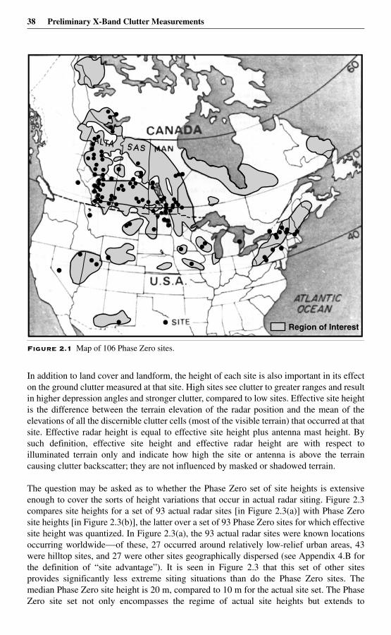
38 Preliminary X-Band Clutter Measurements

In addition to land cover and landform, the height of each site is also important in its effecton the ground clutter measured at that site. High sites see clutter to greater ranges and resultin higher depression angles and stronger clutter, compared to low sites. Effective site heightis the difference between the terrain elevation of the radar position and the mean of theelevations of all the discernible clutter cells (most of the visible terrain) that occurred at thatsite. Effective radar height is equal to effective site height plus antenna mast height. Bysuch definition, effective site height and effective radar height are with respect toilluminated terrain only and indicate how high the site or antenna is above the terraincausing clutter backscatter; they are not influenced by masked or shadowed terrain.

The question may be asked as to whether the Phase Zero set of site heights is extensiveenough to cover the sorts of height variations that occur in actual radar siting. Figure 2.3compares site heights for a set of 93 actual radar sites [in Figure 2.3(a)] with Phase Zerosite heights [in Figure 2.3(b)], the latter over a set of 93 Phase Zero sites for which effectivesite height was quantized. In Figure 2.3(a), the 93 actual radar sites were known locationsoccurring worldwide—of these, 27 occurred around relatively low-relief urban areas, 43were hilltop sites, and 27 were other sites geographically dispersed (see Appendix 4.B forthe definition of “site advantage”). It is seen in Figure 2.3 that this set of other sitesprovides significantly less extreme siting situations than do the Phase Zero sites. Themedian Phase Zero site height is 20 m, compared to 10 m for the actual site set. The PhaseZero site set not only encompasses the regime of actual site heights but extends to

Figure 2.1 Map of 106 Phase Zero sites.

Region of Interest

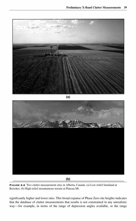
Preliminary X-Band Clutter Measurements 39

significantly higher and lower sites. This broad expanse of Phase Zero site heights indicatesthat the database of clutter measurements that results is not constrained in any unrealisticway—for example, in terms of the range of depression angles available, or the range

Figure 2.2 Two clutter measurement sites in Alberta, Canada. (a) Low-relief farmland at Beiseker. (b) High-relief mountainous terrain at Plateau Mt.

(a)

(b)

40 Preliminary X-Band Clutter Measurements

Table 2.1 Land Cover Classes

Table 2.2 Landform Classes and Descriptions

1 Urban or Built-up Land

11 Residential

12 Commercial

2 Agricultural Land

21 Cropland

22 Pasture

3 Rangeland

31 Herbaceous

32 Shrub

33 Mixed

4 Forest

41 Deciduous

42 Coniferous

43 Mixed

5 Water

51 Rivers, Streams, Canals

52 Lakes, Ponds, Sloughs

6 Wetland

61 Forested

62 Non-Forested

7 Barren Land

1 Level

2 Inclined

3 Undulating

4* Rolling

5 Hummocky

6* Ridged

7* Moderately Steep

8* Steep

9 Broken

Unidirectional

Regular sequences of gentleslopes; wavelike

Regular to irregular sequences ofmoderate slopes

Complex sequences of slopes

Sharp breaks in slope at tops andbottoms of terrain features

Unidirectional

Frequently unidirectional

Short dissected slopes

< 25

> 50

25 — 100

> 150

25 — 100

50 — 500

> 100

> 100

> 50

< 1°

1° – 2°

< 1°

2° – 5°

< 2°

2° – 10°

2° – 10°

10° – 35°

1° – 5°

* Classes so indicated are “high-relief;” classes not so indicated are “low-relief.”

Landform ClassTerrainRelief

(ft)

TerrainSlope(deg)

Comments

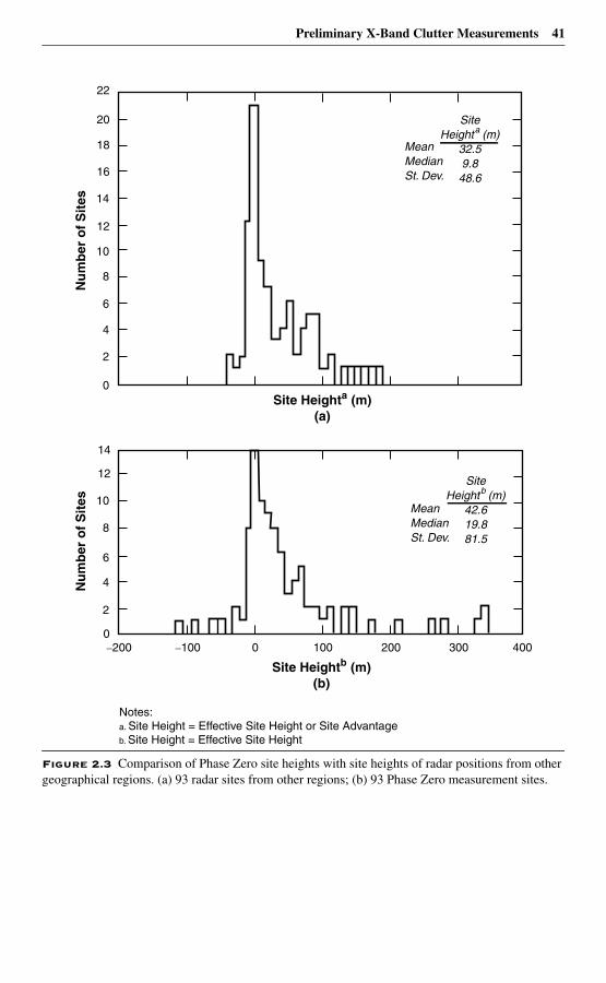
Preliminary X-Band Clutter Measurements 41

Figure 2.3 Comparison of Phase Zero site heights with site heights of radar positions from other geographical regions. (a) 93 radar sites from other regions; (b) 93 Phase Zero measurement sites.

4

2

0

14

16

18

20

22

12

10

8

6

Site Heighta (m)(a)

MeanMedianSt. Dev.

SiteHeighta (m)

32.59.8

48.6

Nu

mb

er o

f S

ites

4

2

0

14

12

10

8

6

–100–200 0 100 400300200

Site Heightb (m)(b)

MeanMedianSt. Dev.

SiteHeightb (m)

42.619.881.5

Nu

mb

er o

f S

ites

Notes:a. Site Height = Effective Site Height or Site Advantageb. Site Height = Effective Site Height

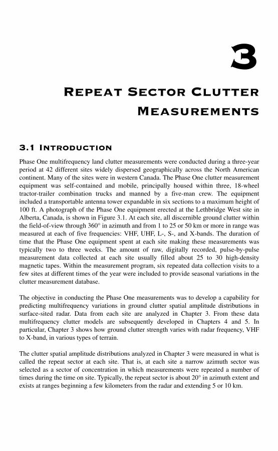
3Repeat Sector Clutter

Measurements

3.1 Introduction Phase One multifrequency land clutter measurements were conducted during a three-yearperiod at 42 different sites widely dispersed geographically across the North Americancontinent. Many of the sites were in western Canada. The Phase One clutter measurementequipment was self-contained and mobile, principally housed within three, 18-wheeltractor-trailer combination trucks and manned by a five-man crew. The equipmentincluded a transportable antenna tower expandable in six sections to a maximum height of100 ft. A photograph of the Phase One equipment erected at the Lethbridge West site inAlberta, Canada, is shown in Figure 3.1. At each site, all discernible ground clutter withinthe field-of-view through 360° in azimuth and from 1 to 25 or 50 km or more in range wasmeasured at each of five frequencies: VHF, UHF, L-, S-, and X-bands. The duration oftime that the Phase One equipment spent at each site making these measurements wastypically two to three weeks. The amount of raw, digitally recorded, pulse-by-pulsemeasurement data collected at each site usually filled about 25 to 30 high-densitymagnetic tapes. Within the measurement program, six repeated data collection visits to afew sites at different times of the year were included to provide seasonal variations in theclutter measurement database.

The objective in conducting the Phase One measurements was to develop a capability forpredicting multifrequency variations in ground clutter spatial amplitude distributions insurface-sited radar. Data from each site are analyzed in Chapter 3. From these datamultifrequency clutter models are subsequently developed in Chapters 4 and 5. Inparticular, Chapter 3 shows how ground clutter strength varies with radar frequency, VHFto X-band, in various types of terrain.

The clutter spatial amplitude distributions analyzed in Chapter 3 were measured in what iscalled the repeat sector at each site. That is, at each site a narrow azimuth sector wasselected as a sector of concentration in which measurements were repeated a number oftimes during the time on site. Typically, the repeat sector is about 20° in azimuth extent andexists at ranges beginning a few kilometers from the radar and extending 5 or 10 km.

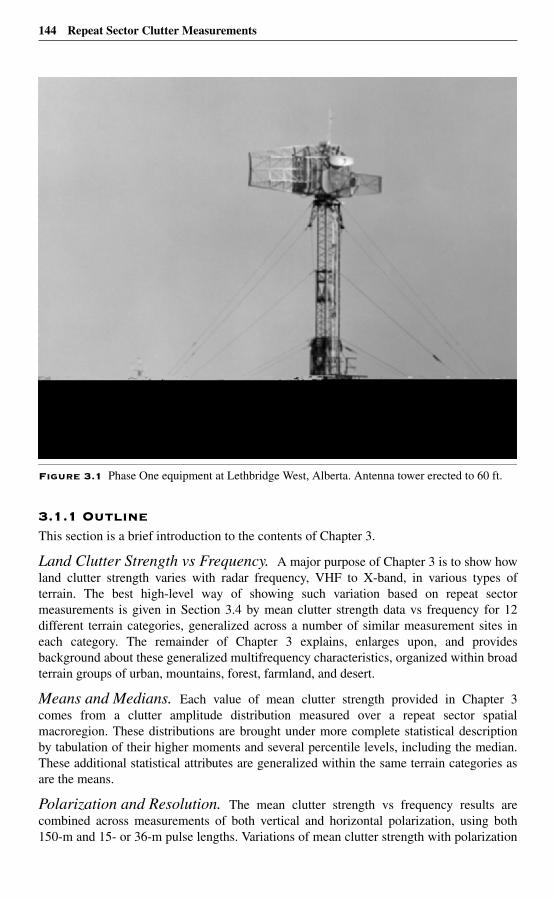
144 Repeat Sector Clutter Measurements

3.1.1 OutlineThis section is a brief introduction to the contents of Chapter 3.

Land Clutter Strength vs Frequency. A major purpose of Chapter 3 is to show howland clutter strength varies with radar frequency, VHF to X-band, in various types ofterrain. The best high-level way of showing such variation based on repeat sectormeasurements is given in Section 3.4 by mean clutter strength data vs frequency for 12different terrain categories, generalized across a number of similar measurement sites ineach category. The remainder of Chapter 3 explains, enlarges upon, and providesbackground about these generalized multifrequency characteristics, organized within broadterrain groups of urban, mountains, forest, farmland, and desert.

Means and Medians. Each value of mean clutter strength provided in Chapter 3comes from a clutter amplitude distribution measured over a repeat sector spatialmacroregion. These distributions are brought under more complete statistical descriptionby tabulation of their higher moments and several percentile levels, including the median.These additional statistical attributes are generalized within the same terrain categories asare the means.

Polarization and Resolution. The mean clutter strength vs frequency results arecombined across measurements of both vertical and horizontal polarization, using both150-m and 15- or 36-m pulse lengths. Variations of mean clutter strength with polarization

Figure 3.1 Phase One equipment at Lethbridge West, Alberta. Antenna tower erected to 60 ft.

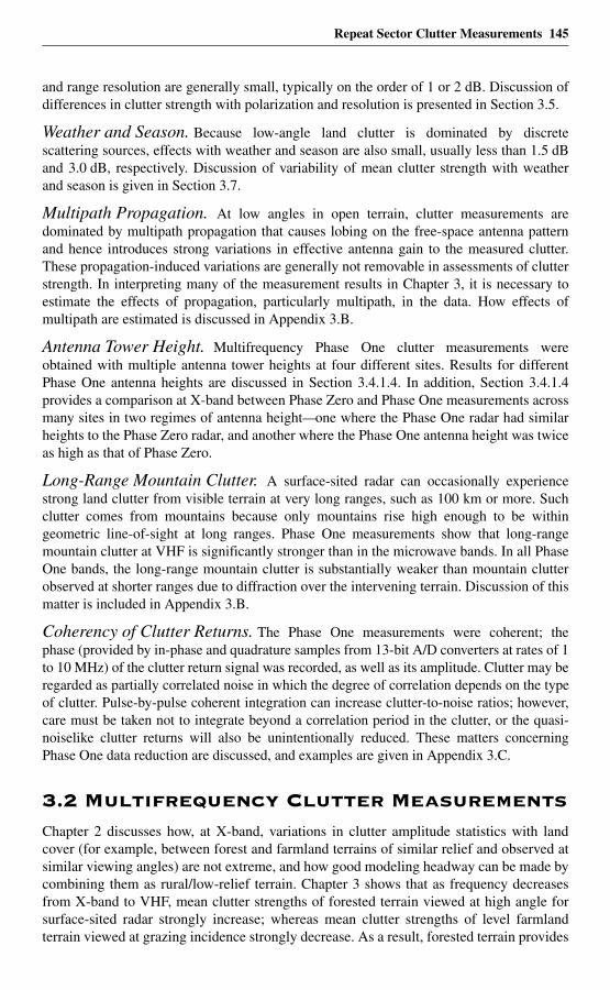
Repeat Sector Clutter Measurements 145

and range resolution are generally small, typically on the order of 1 or 2 dB. Discussion ofdifferences in clutter strength with polarization and resolution is presented in Section 3.5.

Weather and Season. Because low-angle land clutter is dominated by discretescattering sources, effects with weather and season are also small, usually less than 1.5 dBand 3.0 dB, respectively. Discussion of variability of mean clutter strength with weatherand season is given in Section 3.7.

Multipath Propagation. At low angles in open terrain, clutter measurements aredominated by multipath propagation that causes lobing on the free-space antenna patternand hence introduces strong variations in effective antenna gain to the measured clutter.These propagation-induced variations are generally not removable in assessments of clutterstrength. In interpreting many of the measurement results in Chapter 3, it is necessary toestimate the effects of propagation, particularly multipath, in the data. How effects ofmultipath are estimated is discussed in Appendix 3.B.

Antenna Tower Height. Multifrequency Phase One clutter measurements wereobtained with multiple antenna tower heights at four different sites. Results for differentPhase One antenna heights are discussed in Section 3.4.1.4. In addition, Section 3.4.1.4provides a comparison at X-band between Phase Zero and Phase One measurements acrossmany sites in two regimes of antenna height—one where the Phase One radar had similarheights to the Phase Zero radar, and another where the Phase One antenna height was twiceas high as that of Phase Zero.

Long-Range Mountain Clutter. A surface-sited radar can occasionally experiencestrong land clutter from visible terrain at very long ranges, such as 100 km or more. Suchclutter comes from mountains because only mountains rise high enough to be withingeometric line-of-sight at long ranges. Phase One measurements show that long-rangemountain clutter at VHF is significantly stronger than in the microwave bands. In all PhaseOne bands, the long-range mountain clutter is substantially weaker than mountain clutterobserved at shorter ranges due to diffraction over the intervening terrain. Discussion of thismatter is included in Appendix 3.B.

Coherency of Clutter Returns. The Phase One measurements were coherent; thephase (provided by in-phase and quadrature samples from 13-bit A/D converters at rates of 1to 10 MHz) of the clutter return signal was recorded, as well as its amplitude. Clutter may beregarded as partially correlated noise in which the degree of correlation depends on the typeof clutter. Pulse-by-pulse coherent integration can increase clutter-to-noise ratios; however,care must be taken not to integrate beyond a correlation period in the clutter, or the quasi-noiselike clutter returns will also be unintentionally reduced. These matters concerningPhase One data reduction are discussed, and examples are given in Appendix 3.C.

3.2 Multifrequency Clutter MeasurementsChapter 2 discusses how, at X-band, variations in clutter amplitude statistics with landcover (for example, between forest and farmland terrains of similar relief and observed atsimilar viewing angles) are not extreme, and how good modeling headway can be made bycombining them as rural/low-relief terrain. Chapter 3 shows that as frequency decreasesfrom X-band to VHF, mean clutter strengths of forested terrain viewed at high angle forsurface-sited radar strongly increase; whereas mean clutter strengths of level farmlandterrain viewed at grazing incidence strongly decrease. As a result, forested terrain provides

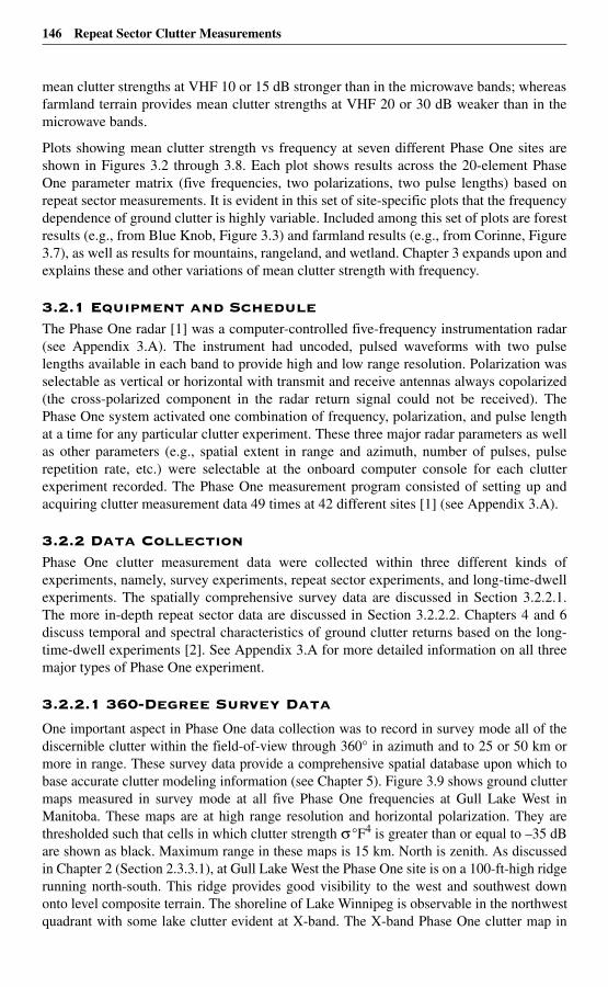
146 Repeat Sector Clutter Measurements

mean clutter strengths at VHF 10 or 15 dB stronger than in the microwave bands; whereasfarmland terrain provides mean clutter strengths at VHF 20 or 30 dB weaker than in themicrowave bands.

Plots showing mean clutter strength vs frequency at seven different Phase One sites areshown in Figures 3.2 through 3.8. Each plot shows results across the 20-element PhaseOne parameter matrix (five frequencies, two polarizations, two pulse lengths) based onrepeat sector measurements. It is evident in this set of site-specific plots that the frequencydependence of ground clutter is highly variable. Included among this set of plots are forestresults (e.g., from Blue Knob, Figure 3.3) and farmland results (e.g., from Corinne, Figure3.7), as well as results for mountains, rangeland, and wetland. Chapter 3 expands upon andexplains these and other variations of mean clutter strength with frequency.

3.2.1 Equipment and ScheduleThe Phase One radar [1] was a computer-controlled five-frequency instrumentation radar(see Appendix 3.A). The instrument had uncoded, pulsed waveforms with two pulselengths available in each band to provide high and low range resolution. Polarization wasselectable as vertical or horizontal with transmit and receive antennas always copolarized(the cross-polarized component in the radar return signal could not be received). ThePhase One system activated one combination of frequency, polarization, and pulse lengthat a time for any particular clutter experiment. These three major radar parameters as wellas other parameters (e.g., spatial extent in range and azimuth, number of pulses, pulserepetition rate, etc.) were selectable at the onboard computer console for each clutterexperiment recorded. The Phase One measurement program consisted of setting up andacquiring clutter measurement data 49 times at 42 different sites [1] (see Appendix 3.A).

3.2.2 Data CollectionPhase One clutter measurement data were collected within three different kinds ofexperiments, namely, survey experiments, repeat sector experiments, and long-time-dwellexperiments. The spatially comprehensive survey data are discussed in Section 3.2.2.1.The more in-depth repeat sector data are discussed in Section 3.2.2.2. Chapters 4 and 6discuss temporal and spectral characteristics of ground clutter returns based on the long-time-dwell experiments [2]. See Appendix 3.A for more detailed information on all threemajor types of Phase One experiment.

3.2.2.1 360-Degree Survey Data

One important aspect in Phase One data collection was to record in survey mode all of thediscernible clutter within the field-of-view through 360° in azimuth and to 25 or 50 km ormore in range. These survey data provide a comprehensive spatial database upon which tobase accurate clutter modeling information (see Chapter 5). Figure 3.9 shows ground cluttermaps measured in survey mode at all five Phase One frequencies at Gull Lake West inManitoba. These maps are at high range resolution and horizontal polarization. They arethresholded such that cells in which clutter strength σ°F4 is greater than or equal to –35 dBare shown as black. Maximum range in these maps is 15 km. North is zenith. As discussedin Chapter 2 (Section 2.3.3.1), at Gull Lake West the Phase One site is on a 100-ft-high ridgerunning north-south. This ridge provides good visibility to the west and southwest downonto level composite terrain. The shoreline of Lake Winnipeg is observable in the northwestquadrant with some lake clutter evident at X-band. The X-band Phase One clutter map in

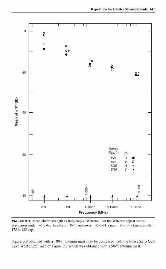
Repeat Sector Clutter Measurements 147

Figure 3.9 obtained with a 100-ft antenna mast may be compared with the Phase Zero GullLake West clutter map of Figure 2.7 which was obtained with a 50-ft antenna mast.

Figure 3.2 Mean clutter strength vs frequency at Waterton. For the Waterton repeat sector, depression angle = –1.8 deg, landform = 8-7, land cover = 42-7-41, range = 9 to 14.9 km, azimuth = 175 to 185 deg.

Frequency (MHz)

100

1,00

0

10,0

00

Range Res. (m) Pol.

150150

15/3615/36

HVHV

0

−20

−40

−60

−80

VHF UHF L-Band S-Band X-Band

Mea

n o

f σ°

F4 (

dB

)

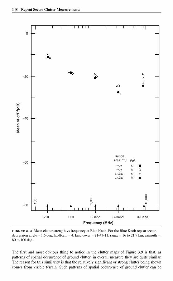
148 Repeat Sector Clutter Measurements

The first and most obvious thing to notice in the clutter maps of Figure 3.9 is that, aspatterns of spatial occurrence of ground clutter, in overall measure they are quite similar.The reason for this similarity is that the relatively significant or strong clutter being showncomes from visible terrain. Such patterns of spatial occurrence of ground clutter can be

Figure 3.3 Mean clutter strength vs frequency at Blue Knob. For the Blue Knob repeat sector, depression angle = 1.6 deg, landform = 4, land cover = 21-43-11, range = 16 to 21.9 km, azimuth = 80 to 100 deg.

Frequency (MHz)

100

1,00

0

10,0

00

Range Res. (m) Pol.

150150

15/3615/36

HVHV

0

−20

−40

−60

−80

VHF UHF L-Band S-Band X-Band

Mea

n o

f σ°

F4 (

dB

)

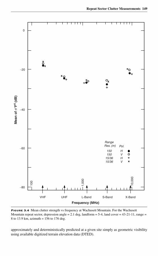
Repeat Sector Clutter Measurements 149

approximately and deterministically predicted at a given site simply as geometric visibilityusing available digitized terrain elevation data (DTED).

Figure 3.4 Mean clutter strength vs frequency at Wachusett Mountain. For the Wachusett Mountain repeat sector, depression angle = 2.1 deg, landform = 5-4, land cover = 43-21-11, range = 8 to 13.9 km, azimuth = 156 to 176 deg.

Frequency (MHz)

100

1,00

0

10,0

00

0

−20

−40

−60

−80

VHF UHF L-Band S-Band X-Band

Mea

n o

f σ°

F4

(dB

)

Range Res. (m) Pol.

150150

15/3615/36

HVHV

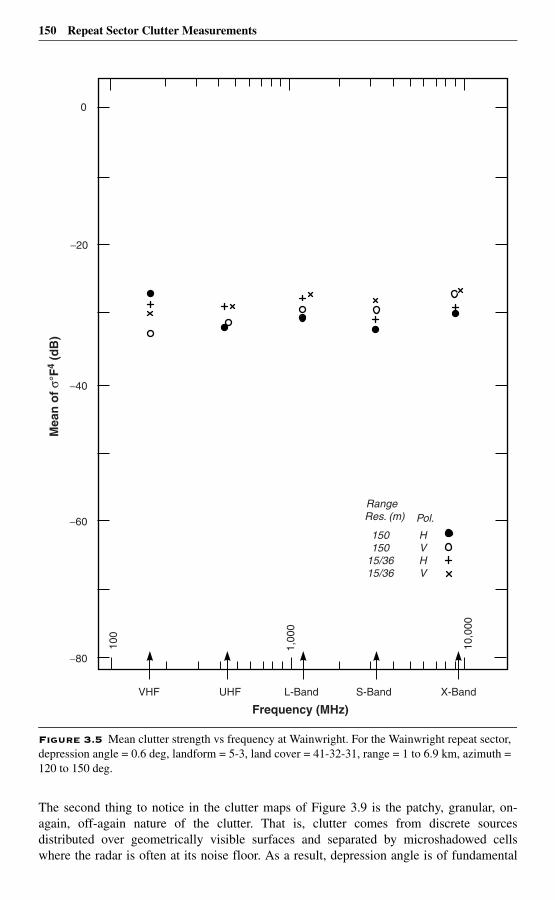
150 Repeat Sector Clutter Measurements

The second thing to notice in the clutter maps of Figure 3.9 is the patchy, granular, on-again, off-again nature of the clutter. That is, clutter comes from discrete sourcesdistributed over geometrically visible surfaces and separated by microshadowed cellswhere the radar is often at its noise floor. As a result, depression angle is of fundamental

Figure 3.5 Mean clutter strength vs frequency at Wainwright. For the Wainwright repeat sector, depression angle = 0.6 deg, landform = 5-3, land cover = 41-32-31, range = 1 to 6.9 km, azimuth = 120 to 150 deg.

Frequency (MHz)

100

1,00

0

10,0

00

0

−20

−40

−60

−80

VHF UHF L-Band S-Band X-Band

Mea

n o

f σ°

F4

(dB

)

Range Res. (m) Pol.

150150

15/3615/36

HVHV

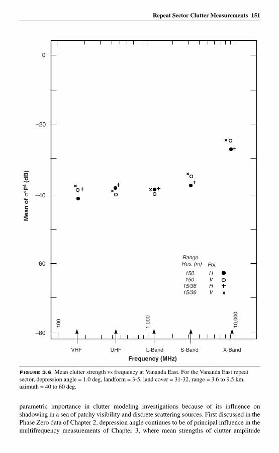
Repeat Sector Clutter Measurements 151

parametric importance in clutter modeling investigations because of its influence onshadowing in a sea of patchy visibility and discrete scattering sources. First discussed in thePhase Zero data of Chapter 2, depression angle continues to be of principal influence in themultifrequency measurements of Chapter 3, where mean strengths of clutter amplitude

Figure 3.6 Mean clutter strength vs frequency at Vananda East. For the Vananda East repeat sector, depression angle = 1.0 deg, landform = 3-5, land cover = 31-32, range = 3.6 to 9.5 km, azimuth = 40 to 60 deg.

Frequency (MHz)

100

1,00

0

10,0

00

0

–20

–40

–60

–80

VHF UHF L-Band S-Band X-Band

Mea

n o

f σ°

F4

(dB

)

Range Res. (m) Pol.

150150

15/3615/36

HVHV

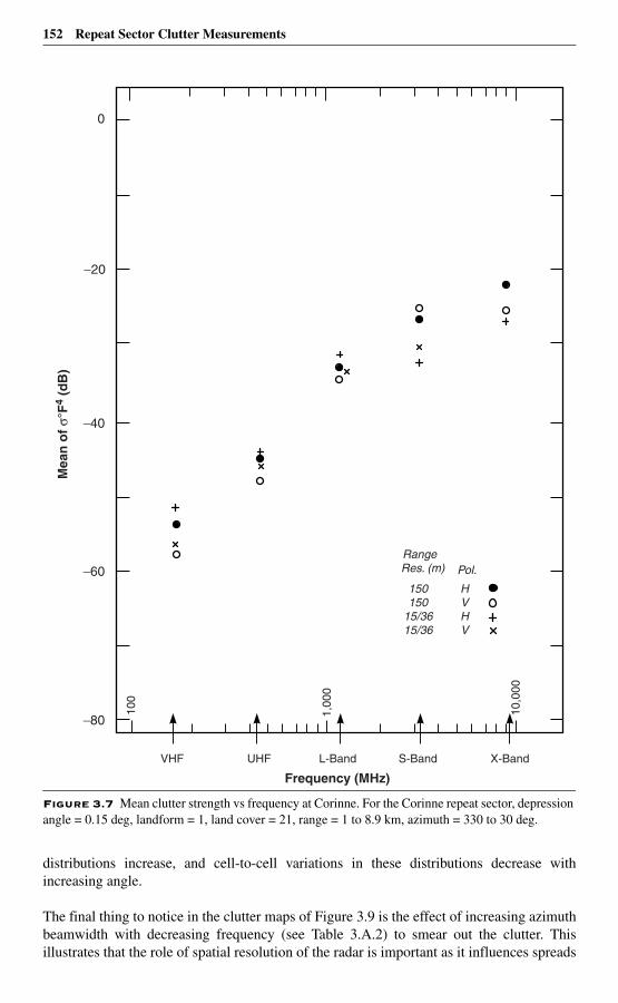
152 Repeat Sector Clutter Measurements

distributions increase, and cell-to-cell variations in these distributions decrease withincreasing angle.

The final thing to notice in the clutter maps of Figure 3.9 is the effect of increasing azimuthbeamwidth with decreasing frequency (see Table 3.A.2) to smear out the clutter. Thisillustrates that the role of spatial resolution of the radar is important as it influences spreads

Figure 3.7 Mean clutter strength vs frequency at Corinne. For the Corinne repeat sector, depression angle = 0.15 deg, landform = 1, land cover = 21, range = 1 to 8.9 km, azimuth = 330 to 30 deg.

Frequency (MHz)

100

1,00

0

10,0

00

0

−20

−40

−60

−80

VHF UHF L-Band S-Band X-Band

Mea

n o

f σ°

F4

(dB

)

Range Res. (m) Pol.

150150

15/3615/36

HVHV

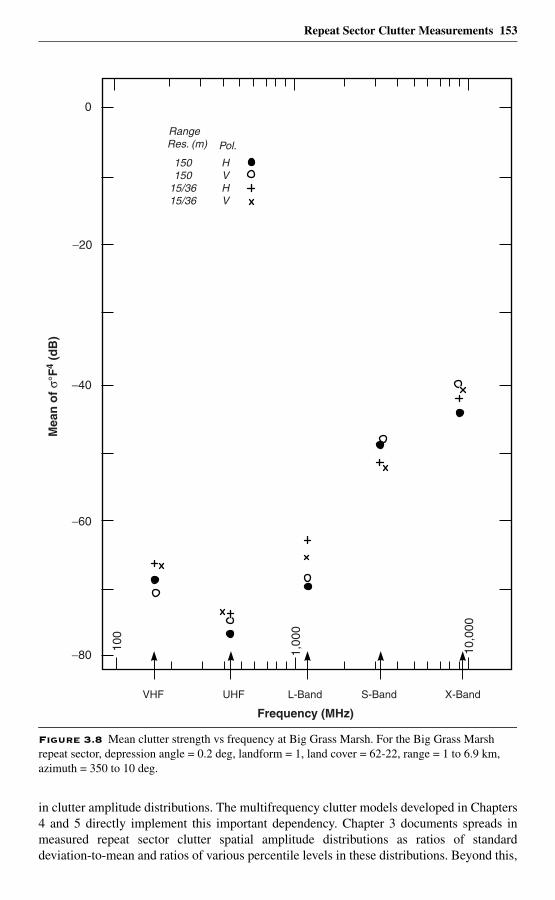
Repeat Sector Clutter Measurements 153

in clutter amplitude distributions. The multifrequency clutter models developed in Chapters4 and 5 directly implement this important dependency. Chapter 3 documents spreads inmeasured repeat sector clutter spatial amplitude distributions as ratios of standarddeviation-to-mean and ratios of various percentile levels in these distributions. Beyond this,

Figure 3.8 Mean clutter strength vs frequency at Big Grass Marsh. For the Big Grass Marsh repeat sector, depression angle = 0.2 deg, landform = 1, land cover = 62-22, range = 1 to 6.9 km, azimuth = 350 to 10 deg.

Frequency (MHz)

100

1,00

0

10,0

00

0

−20

−40

−60

−80

VHF UHF L-Band S-Band X-Band

Mea

n o

f σ°

F4

(dB

)

Range Res. (m) Pol.

150150

15/3615/36

HVHV

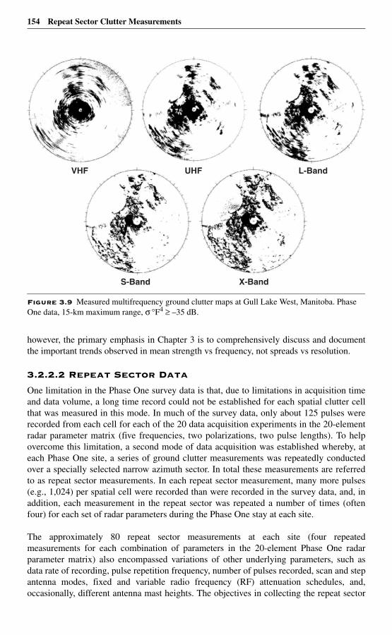
154 Repeat Sector Clutter Measurements

however, the primary emphasis in Chapter 3 is to comprehensively discuss and documentthe important trends observed in mean strength vs frequency, not spreads vs resolution.

3.2.2.2 Repeat Sector Data

One limitation in the Phase One survey data is that, due to limitations in acquisition timeand data volume, a long time record could not be established for each spatial clutter cellthat was measured in this mode. In much of the survey data, only about 125 pulses wererecorded from each cell for each of the 20 data acquisition experiments in the 20-elementradar parameter matrix (five frequencies, two polarizations, two pulse lengths). To helpovercome this limitation, a second mode of data acquisition was established whereby, ateach Phase One site, a series of ground clutter measurements was repeatedly conductedover a specially selected narrow azimuth sector. In total these measurements are referredto as repeat sector measurements. In each repeat sector measurement, many more pulses(e.g., 1,024) per spatial cell were recorded than were recorded in the survey data, and, inaddition, each measurement in the repeat sector was repeated a number of times (oftenfour) for each set of radar parameters during the Phase One stay at each site.

The approximately 80 repeat sector measurements at each site (four repeatedmeasurements for each combination of parameters in the 20-element Phase One radarparameter matrix) also encompassed variations of other underlying parameters, such asdata rate of recording, pulse repetition frequency, number of pulses recorded, scan and stepantenna modes, fixed and variable radio frequency (RF) attenuation schedules, and,occasionally, different antenna mast heights. The objectives in collecting the repeat sector

Figure 3.9 Measured multifrequency ground clutter maps at Gull Lake West, Manitoba. Phase One data, 15-km maximum range, σ °F4 ≥ –35 dB.

S-Band X-Band

L-BandUHFVHF

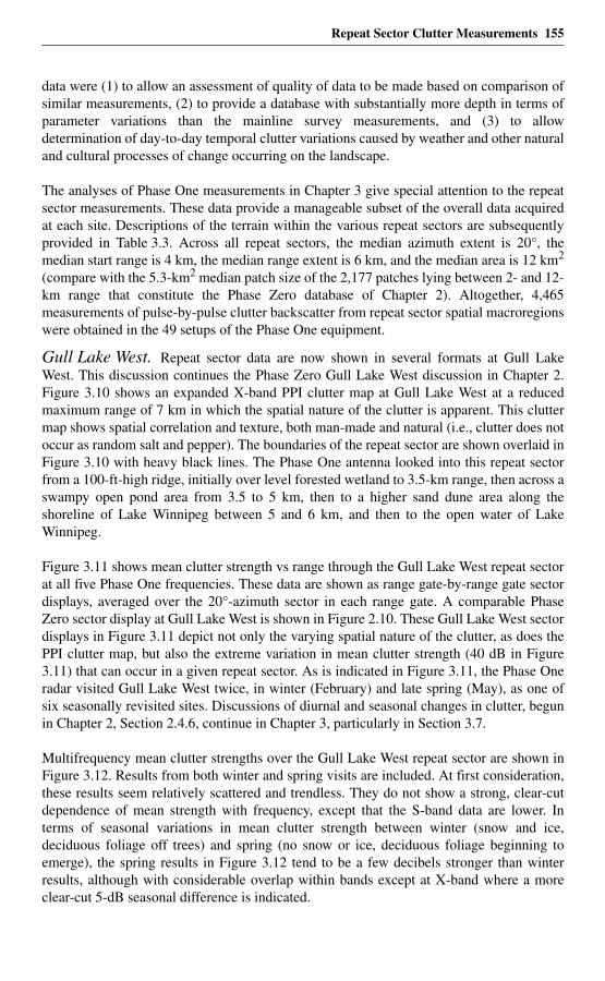
Repeat Sector Clutter Measurements 155

data were (1) to allow an assessment of quality of data to be made based on comparison ofsimilar measurements, (2) to provide a database with substantially more depth in terms ofparameter variations than the mainline survey measurements, and (3) to allowdetermination of day-to-day temporal clutter variations caused by weather and other naturaland cultural processes of change occurring on the landscape.

The analyses of Phase One measurements in Chapter 3 give special attention to the repeatsector measurements. These data provide a manageable subset of the overall data acquiredat each site. Descriptions of the terrain within the various repeat sectors are subsequentlyprovided in Table 3.3. Across all repeat sectors, the median azimuth extent is 20°, themedian start range is 4 km, the median range extent is 6 km, and the median area is 12 km2

(compare with the 5.3-km2 median patch size of the 2,177 patches lying between 2- and 12-km range that constitute the Phase Zero database of Chapter 2). Altogether, 4,465measurements of pulse-by-pulse clutter backscatter from repeat sector spatial macroregionswere obtained in the 49 setups of the Phase One equipment.

Gull Lake West. Repeat sector data are now shown in several formats at Gull LakeWest. This discussion continues the Phase Zero Gull Lake West discussion in Chapter 2.Figure 3.10 shows an expanded X-band PPI clutter map at Gull Lake West at a reducedmaximum range of 7 km in which the spatial nature of the clutter is apparent. This cluttermap shows spatial correlation and texture, both man-made and natural (i.e., clutter does notoccur as random salt and pepper). The boundaries of the repeat sector are shown overlaid inFigure 3.10 with heavy black lines. The Phase One antenna looked into this repeat sectorfrom a 100-ft-high ridge, initially over level forested wetland to 3.5-km range, then across aswampy open pond area from 3.5 to 5 km, then to a higher sand dune area along theshoreline of Lake Winnipeg between 5 and 6 km, and then to the open water of LakeWinnipeg.

Figure 3.11 shows mean clutter strength vs range through the Gull Lake West repeat sectorat all five Phase One frequencies. These data are shown as range gate-by-range gate sectordisplays, averaged over the 20°-azimuth sector in each range gate. A comparable PhaseZero sector display at Gull Lake West is shown in Figure 2.10. These Gull Lake West sectordisplays in Figure 3.11 depict not only the varying spatial nature of the clutter, as does thePPI clutter map, but also the extreme variation in mean clutter strength (40 dB in Figure3.11) that can occur in a given repeat sector. As is indicated in Figure 3.11, the Phase Oneradar visited Gull Lake West twice, in winter (February) and late spring (May), as one ofsix seasonally revisited sites. Discussions of diurnal and seasonal changes in clutter, begunin Chapter 2, Section 2.4.6, continue in Chapter 3, particularly in Section 3.7.

Multifrequency mean clutter strengths over the Gull Lake West repeat sector are shown inFigure 3.12. Results from both winter and spring visits are included. At first consideration,these results seem relatively scattered and trendless. They do not show a strong, clear-cutdependence of mean strength with frequency, except that the S-band data are lower. Interms of seasonal variations in mean clutter strength between winter (snow and ice,deciduous foliage off trees) and spring (no snow or ice, deciduous foliage beginning toemerge), the spring results in Figure 3.12 tend to be a few decibels stronger than winterresults, although with considerable overlap within bands except at X-band where a moreclear-cut 5-dB seasonal difference is indicated.

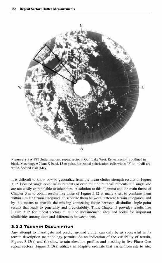
156 Repeat Sector Clutter Measurements

It is difficult to know how to generalize from the mean clutter strength results of Figure3.12. Isolated single-point measurements or even multipoint measurements at a single siteare not easily extrapolable to other sites. A solution to this dilemma and the main thrust ofChapter 3 is to obtain results like those of Figure 3.12 at many sites, to combine themwithin similar terrain categories, to separate them between different terrain categories, andby this means to provide the missing connecting tissue between dissimilar single-pointresults that leads to generality and predictability. Thus, Chapter 3 provides results likeFigure 3.12 for repeat sectors at all the measurement sites and looks for importantsimilarities among them and differences between them.

3.2.3 Terrain DescriptionAny attempt to investigate and predict ground clutter can only be as successful as itsterrain description methodology permits. As an indication of the variability of terrain,Figures 3.13(a) and (b) show terrain elevation profiles and masking in five Phase Onerepeat sectors [Figure 3.13(a) utilizes an adaptive ordinate that varies from site to site;

Figure 3.10 PPI clutter map and repeat sector at Gull Lake West. Repeat sector is outlined in black. Max range = 7 km; X-band, 15-m pulse, horizontal polarization; cells with σ °F4 ≥ –40 dB are white. Second visit (May).

N

S

W E

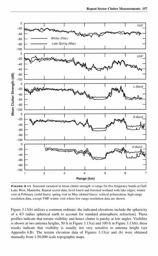
Repeat Sector Clutter Measurements 157

Figure 3.13(b) utilizes a common ordinate; the indicated elevations include the sphericityof a 4/3 radius spherical earth to account for standard atmospheric refraction]. Theseprofiles indicate that terrain visibility and hence clutter is patchy at low angles. Visibilityis shown at two antenna heights, 50 ft in Figure 3.13(a) and 100 ft in Figure 3.13(b); theseresults indicate that visibility is usually not very sensitive to antenna height (seeAppendix 4.B). The terrain elevation data of Figures 3.13(a) and (b) were obtainedmanually from 1:50,000 scale topographic maps.

Figure 3.11 Seasonal variation in mean clutter strength vs range for five frequency bands at Gull Lake West, Manitoba. Repeat sector data; level forest and forested wetland with lake edges; winter visit in February (solid lines), spring visit in May (dotted lines); vertical polarization, high range resolution data, except VHF winter visit where low range resolution data are shown.

Mea

n C

lutt

er S

tren

gth

(d

B)

Range (km)

L-Band

S-Band

UHF

VHF

X-Band

Winter (Feb.)

Late Spring (May)

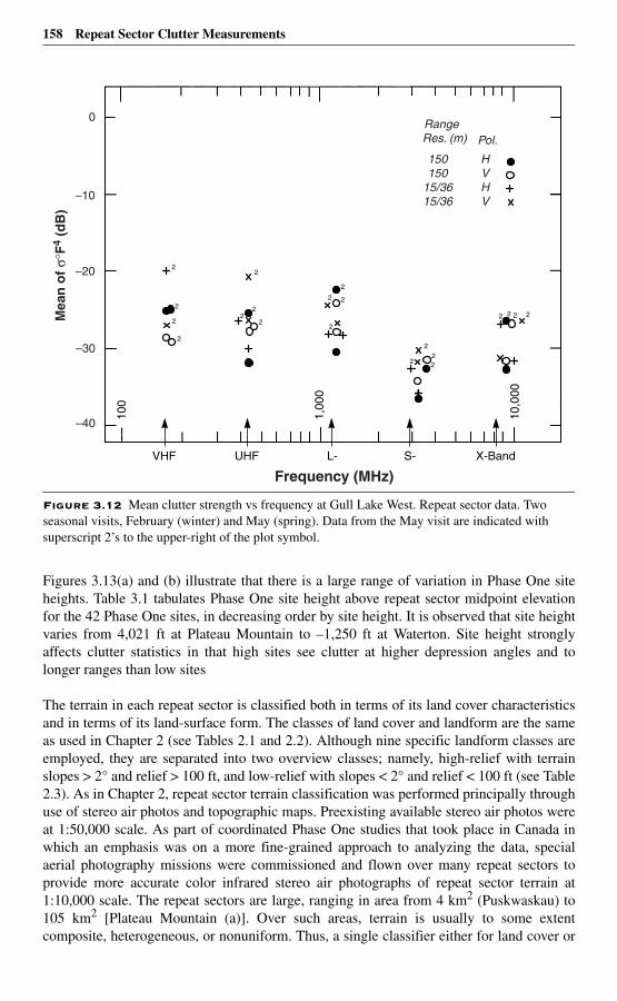
158 Repeat Sector Clutter Measurements

Figures 3.13(a) and (b) illustrate that there is a large range of variation in Phase One siteheights. Table 3.1 tabulates Phase One site height above repeat sector midpoint elevationfor the 42 Phase One sites, in decreasing order by site height. It is observed that site heightvaries from 4,021 ft at Plateau Mountain to –1,250 ft at Waterton. Site height stronglyaffects clutter statistics in that high sites see clutter at higher depression angles and tolonger ranges than low sites

The terrain in each repeat sector is classified both in terms of its land cover characteristicsand in terms of its land-surface form. The classes of land cover and landform are the sameas used in Chapter 2 (see Tables 2.1 and 2.2). Although nine specific landform classes areemployed, they are separated into two overview classes; namely, high-relief with terrainslopes > 2° and relief > 100 ft, and low-relief with slopes < 2° and relief < 100 ft (see Table2.3). As in Chapter 2, repeat sector terrain classification was performed principally throughuse of stereo air photos and topographic maps. Preexisting available stereo air photos wereat 1:50,000 scale. As part of coordinated Phase One studies that took place in Canada inwhich an emphasis was on a more fine-grained approach to analyzing the data, specialaerial photography missions were commissioned and flown over many repeat sectors toprovide more accurate color infrared stereo air photographs of repeat sector terrain at1:10,000 scale. The repeat sectors are large, ranging in area from 4 km2 (Puskwaskau) to105 km2 [Plateau Mountain (a)]. Over such areas, terrain is usually to some extentcomposite, heterogeneous, or nonuniform. Thus, a single classifier either for land cover or

Figure 3.12 Mean clutter strength vs frequency at Gull Lake West. Repeat sector data. Two seasonal visits, February (winter) and May (spring). Data from the May visit are indicated with superscript 2’s to the upper-right of the plot symbol.

Frequency (MHz)

0

–10

–20

–30

–40

Mea

n o

f σ°

F4

(dB

)

Range Res. (m) Pol.

150150

15/3615/36

HVHV

2

2

2

2

2

2

2

22

2

2

2

2

2

22

S- X-BandL-UHFVHF

10,0

00

1,00

0

100

2

2 2 2

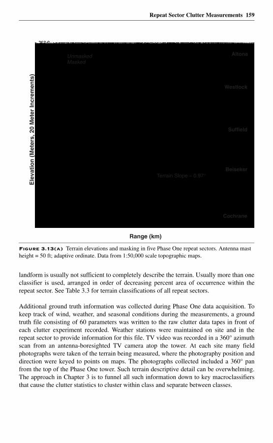
Repeat Sector Clutter Measurements 159

landform is usually not sufficient to completely describe the terrain. Usually more than oneclassifier is used, arranged in order of decreasing percent area of occurrence within therepeat sector. See Table 3.3 for terrain classifications of all repeat sectors.

Additional ground truth information was collected during Phase One data acquisition. Tokeep track of wind, weather, and seasonal conditions during the measurements, a groundtruth file consisting of 60 parameters was written to the raw clutter data tapes in front ofeach clutter experiment recorded. Weather stations were maintained on site and in therepeat sector to provide information for this file. TV video was recorded in a 360° azimuthscan from an antenna-boresighted TV camera atop the tower. At each site many fieldphotographs were taken of the terrain being measured, where the photography position anddirection were keyed to points on maps. The photographs collected included a 360° panfrom the top of the Phase One tower. Such terrain descriptive detail can be overwhelming.The approach in Chapter 3 is to funnel all such information down to key macroclassifiersthat cause the clutter statistics to cluster within class and separate between classes.

Figure 3.13(a) Terrain elevations and masking in five Phase One repeat sectors. Antenna mast height = 50 ft; adaptive ordinate. Data from 1:50,000 scale topographic maps.

Terrain Slope ≈ 0.97°

UnmaskedMasked

Ele

vati

on

(M

eter

s, 2

0 M

eter

Incr

emen

ts)

Altona

Westlock

Suffield

Beiseker

Cochrane

Range (km)

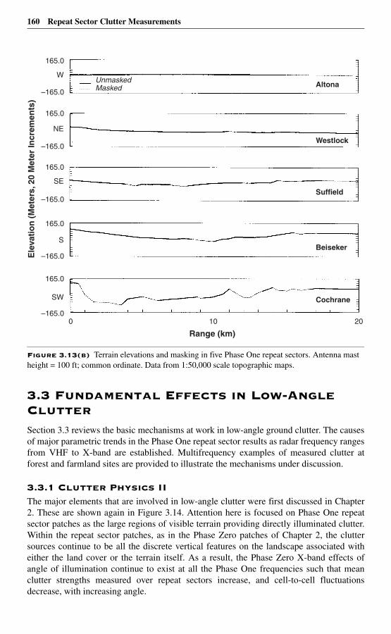
160 Repeat Sector Clutter Measurements

3.3 Fundamental Effects in Low-Angle ClutterSection 3.3 reviews the basic mechanisms at work in low-angle ground clutter. The causesof major parametric trends in the Phase One repeat sector results as radar frequency rangesfrom VHF to X-band are established. Multifrequency examples of measured clutter atforest and farmland sites are provided to illustrate the mechanisms under discussion.

3.3.1 Clutter Physics IIThe major elements that are involved in low-angle clutter were first discussed in Chapter2. These are shown again in Figure 3.14. Attention here is focused on Phase One repeatsector patches as the large regions of visible terrain providing directly illuminated clutter.Within the repeat sector patches, as in the Phase Zero patches of Chapter 2, the cluttersources continue to be all the discrete vertical features on the landscape associated witheither the land cover or the terrain itself. As a result, the Phase Zero X-band effects ofangle of illumination continue to exist at all the Phase One frequencies such that meanclutter strengths measured over repeat sectors increase, and cell-to-cell fluctuationsdecrease, with increasing angle.

Figure 3.13(b) Terrain elevations and masking in five Phase One repeat sectors. Antenna mast height = 100 ft; common ordinate. Data from 1:50,000 scale topographic maps.

165.0

–165.0

W

165.0

–165.0

NE

165.0

–165.0

SE

165.0

–165.0

S

165.0

–165.0

SW

Ele

vati

on

(M

eter

s, 2

0 M

eter

Incr

emen

ts)

0 10 20

Range (km)

Cochrane

Beiseker

Suffield

Westlock

AltonaUnmaskedMasked

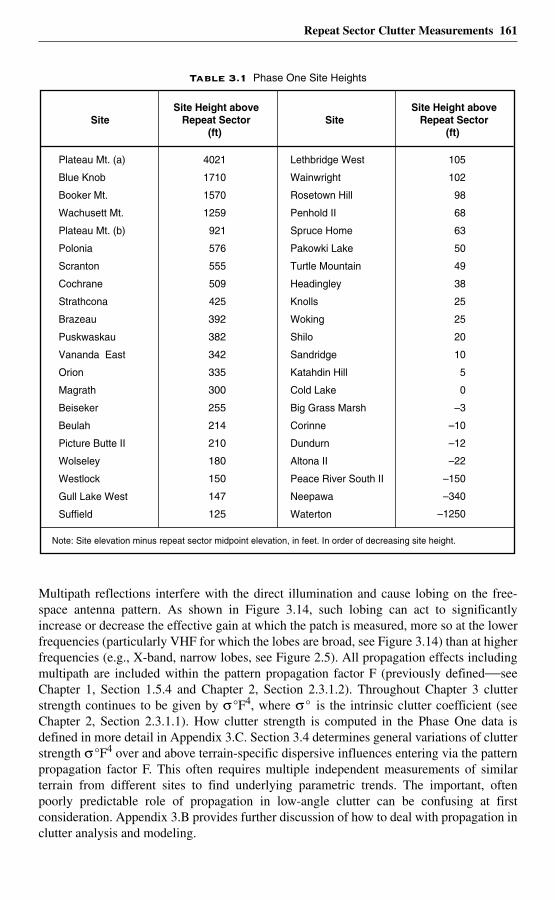
Repeat Sector Clutter Measurements 161

Multipath reflections interfere with the direct illumination and cause lobing on the free-space antenna pattern. As shown in Figure 3.14, such lobing can act to significantlyincrease or decrease the effective gain at which the patch is measured, more so at the lowerfrequencies (particularly VHF for which the lobes are broad, see Figure 3.14) than at higherfrequencies (e.g., X-band, narrow lobes, see Figure 2.5). All propagation effects includingmultipath are included within the pattern propagation factor F (previously defined—seeChapter 1, Section 1.5.4 and Chapter 2, Section 2.3.1.2). Throughout Chapter 3 clutterstrength continues to be given by σ°F4, where σ° is the intrinsic clutter coefficient (seeChapter 2, Section 2.3.1.1). How clutter strength is computed in the Phase One data isdefined in more detail in Appendix 3.C. Section 3.4 determines general variations of clutterstrength σ°F4 over and above terrain-specific dispersive influences entering via the patternpropagation factor F. This often requires multiple independent measurements of similarterrain from different sites to find underlying parametric trends. The important, oftenpoorly predictable role of propagation in low-angle clutter can be confusing at firstconsideration. Appendix 3.B provides further discussion of how to deal with propagation inclutter analysis and modeling.

Table 3.1 Phase One Site Heights

SiteSite Height above

Repeat Sector(ft)

SiteSite Height above

Repeat Sector(ft)

Plateau Mt. (a)

Blue Knob

Booker Mt.

Wachusett Mt.

Plateau Mt. (b)

Polonia

Scranton

Cochrane

Strathcona

Brazeau

Puskwaskau

Vananda East

Orion

Magrath

Beiseker

Beulah

Picture Butte II

Wolseley

Westlock

Gull Lake West

Suffield

4021

1710

1570

1259

921

576

555

509

425

392

382

342

335

300

255

214

210

180

150

147

125

105

102

98

68

63

50

49

38

25

25

20

10

5

0

–3

–10

–12

–22

–150

–340

–1250

Lethbridge West

Wainwright

Rosetown Hill

Penhold II

Spruce Home

Pakowki Lake

Turtle Mountain

Headingley

Knolls

Woking

Shilo

Sandridge

Katahdin Hill

Cold Lake

Big Grass Marsh

Corinne

Dundurn

Altona II

Peace River South II

Neepawa

Waterton

Note: Site elevation minus repeat sector midpoint elevation, in feet. In order of decreasing site height.

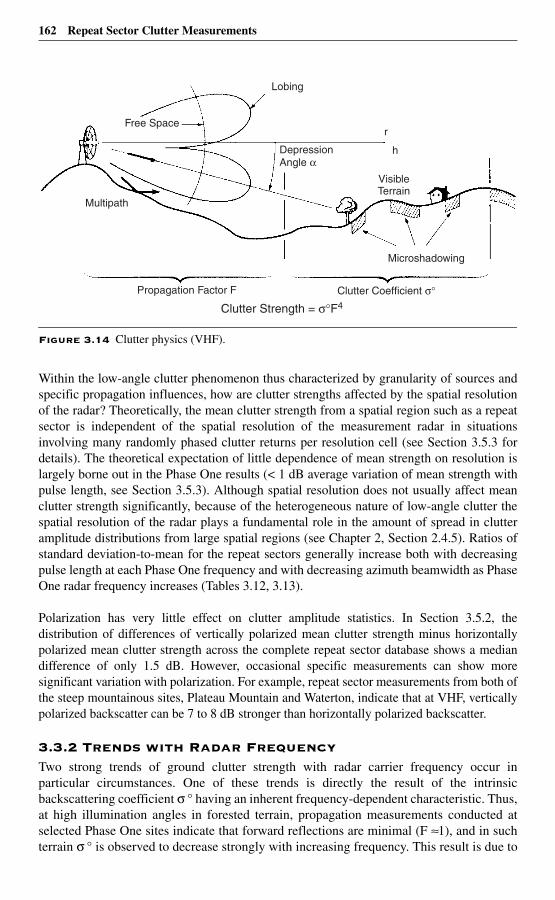
162 Repeat Sector Clutter Measurements

Within the low-angle clutter phenomenon thus characterized by granularity of sources andspecific propagation influences, how are clutter strengths affected by the spatial resolutionof the radar? Theoretically, the mean clutter strength from a spatial region such as a repeatsector is independent of the spatial resolution of the measurement radar in situationsinvolving many randomly phased clutter returns per resolution cell (see Section 3.5.3 fordetails). The theoretical expectation of little dependence of mean strength on resolution islargely borne out in the Phase One results (< 1 dB average variation of mean strength withpulse length, see Section 3.5.3). Although spatial resolution does not usually affect meanclutter strength significantly, because of the heterogeneous nature of low-angle clutter thespatial resolution of the radar plays a fundamental role in the amount of spread in clutteramplitude distributions from large spatial regions (see Chapter 2, Section 2.4.5). Ratios ofstandard deviation-to-mean for the repeat sectors generally increase both with decreasingpulse length at each Phase One frequency and with decreasing azimuth beamwidth as PhaseOne radar frequency increases (Tables 3.12, 3.13).

Polarization has very little effect on clutter amplitude statistics. In Section 3.5.2, thedistribution of differences of vertically polarized mean clutter strength minus horizontallypolarized mean clutter strength across the complete repeat sector database shows a mediandifference of only 1.5 dB. However, occasional specific measurements can show moresignificant variation with polarization. For example, repeat sector measurements from both ofthe steep mountainous sites, Plateau Mountain and Waterton, indicate that at VHF, verticallypolarized backscatter can be 7 to 8 dB stronger than horizontally polarized backscatter.

3.3.2 Trends with Radar FrequencyTwo strong trends of ground clutter strength with radar carrier frequency occur inparticular circumstances. One of these trends is directly the result of the intrinsicbackscattering coefficient σ ° having an inherent frequency-dependent characteristic. Thus,at high illumination angles in forested terrain, propagation measurements conducted atselected Phase One sites indicate that forward reflections are minimal (F ≈1), and in suchterrain σ ° is observed to decrease strongly with increasing frequency. This result is due to

Figure 3.14 Clutter physics (VHF).

Propagation Factor F Clutter Coefficient σ°

Microshadowing

Lobing

Free Space

Multipath

DepressionAngle α

VisibleTerrain

h

r

Clutter Strength = σ°F4

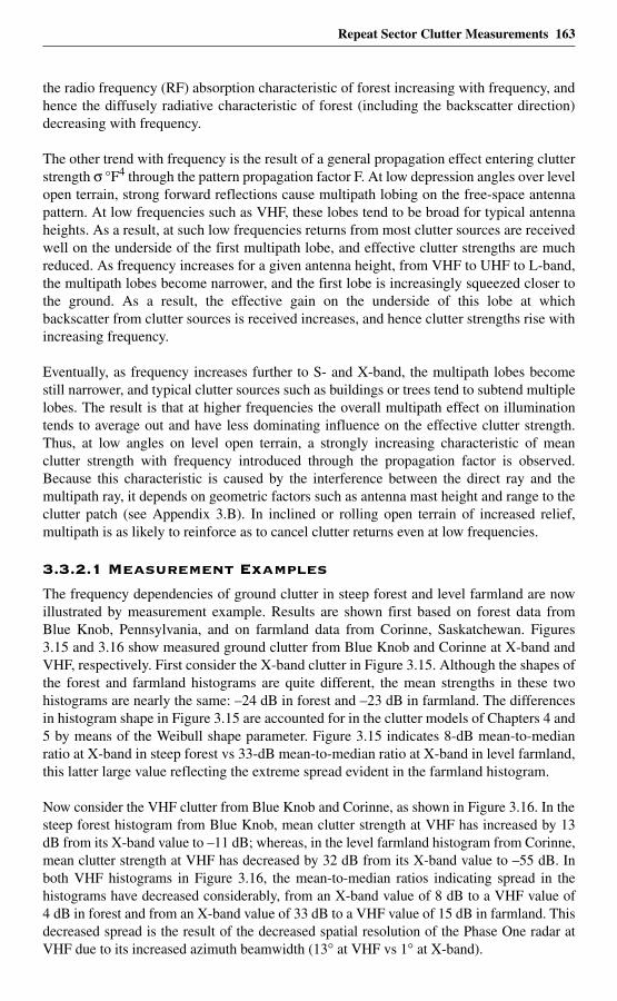
Repeat Sector Clutter Measurements 163

the radio frequency (RF) absorption characteristic of forest increasing with frequency, andhence the diffusely radiative characteristic of forest (including the backscatter direction)decreasing with frequency.

The other trend with frequency is the result of a general propagation effect entering clutterstrength σ °F4 through the pattern propagation factor F. At low depression angles over levelopen terrain, strong forward reflections cause multipath lobing on the free-space antennapattern. At low frequencies such as VHF, these lobes tend to be broad for typical antennaheights. As a result, at such low frequencies returns from most clutter sources are receivedwell on the underside of the first multipath lobe, and effective clutter strengths are muchreduced. As frequency increases for a given antenna height, from VHF to UHF to L-band,the multipath lobes become narrower, and the first lobe is increasingly squeezed closer tothe ground. As a result, the effective gain on the underside of this lobe at whichbackscatter from clutter sources is received increases, and hence clutter strengths rise withincreasing frequency.

Eventually, as frequency increases further to S- and X-band, the multipath lobes becomestill narrower, and typical clutter sources such as buildings or trees tend to subtend multiplelobes. The result is that at higher frequencies the overall multipath effect on illuminationtends to average out and have less dominating influence on the effective clutter strength.Thus, at low angles on level open terrain, a strongly increasing characteristic of meanclutter strength with frequency introduced through the propagation factor is observed.Because this characteristic is caused by the interference between the direct ray and themultipath ray, it depends on geometric factors such as antenna mast height and range to theclutter patch (see Appendix 3.B). In inclined or rolling open terrain of increased relief,multipath is as likely to reinforce as to cancel clutter returns even at low frequencies.

3.3.2.1 Measurement Examples

The frequency dependencies of ground clutter in steep forest and level farmland are nowillustrated by measurement example. Results are shown first based on forest data fromBlue Knob, Pennsylvania, and on farmland data from Corinne, Saskatchewan. Figures3.15 and 3.16 show measured ground clutter from Blue Knob and Corinne at X-band andVHF, respectively. First consider the X-band clutter in Figure 3.15. Although the shapes ofthe forest and farmland histograms are quite different, the mean strengths in these twohistograms are nearly the same: –24 dB in forest and –23 dB in farmland. The differencesin histogram shape in Figure 3.15 are accounted for in the clutter models of Chapters 4 and5 by means of the Weibull shape parameter. Figure 3.15 indicates 8-dB mean-to-medianratio at X-band in steep forest vs 33-dB mean-to-median ratio at X-band in level farmland,this latter large value reflecting the extreme spread evident in the farmland histogram.

Now consider the VHF clutter from Blue Knob and Corinne, as shown in Figure 3.16. In thesteep forest histogram from Blue Knob, mean clutter strength at VHF has increased by 13dB from its X-band value to –11 dB; whereas, in the level farmland histogram from Corinne,mean clutter strength at VHF has decreased by 32 dB from its X-band value to –55 dB. Inboth VHF histograms in Figure 3.16, the mean-to-median ratios indicating spread in thehistograms have decreased considerably, from an X-band value of 8 dB to a VHF value of4 dB in forest and from an X-band value of 33 dB to a VHF value of 15 dB in farmland. Thisdecreased spread is the result of the decreased spatial resolution of the Phase One radar atVHF due to its increased azimuth beamwidth (13° at VHF vs 1° at X-band).

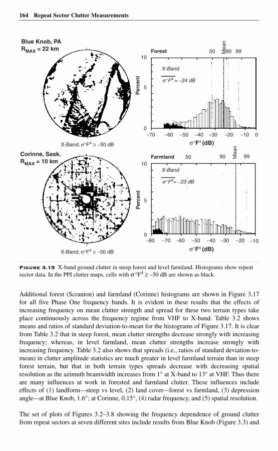
164 Repeat Sector Clutter Measurements

Additional forest (Scranton) and farmland (Corinne) histograms are shown in Figure 3.17for all five Phase One frequency bands. It is evident in these results that the effects ofincreasing frequency on mean clutter strength and spread for these two terrain types takeplace continuously across the frequency regime from VHF to X-band. Table 3.2 showsmeans and ratios of standard deviation-to-mean for the histograms of Figure 3.17. It is clearfrom Table 3.2 that in steep forest, mean clutter strengths decrease strongly with increasingfrequency; whereas, in level farmland, mean clutter strengths increase strongly withincreasing frequency. Table 3.2 also shows that spreads (i.e., ratios of standard deviation-to-mean) in clutter amplitude statistics are much greater in level farmland terrain than in steepforest terrain, but that in both terrain types spreads decrease with decreasing spatialresolution as the azimuth beamwidth increases from 1° at X-band to 13° at VHF. Thus thereare many influences at work in forested and farmland clutter. These influences includeeffects of (1) landform—steep vs level, (2) land cover—forest vs farmland, (3) depressionangle—at Blue Knob, 1.6°; at Corinne, 0.15°, (4) radar frequency, and (5) spatial resolution.

The set of plots of Figures 3.2–3.8 showing the frequency dependence of ground clutterfrom repeat sectors at seven different sites include results from Blue Knob (Figure 3.3) and

Figure 3.15 X-band ground clutter in steep forest and level farmland. Histograms show repeat sector data. In the PPI clutter maps, cells with σ °F4 ≥ –50 dB are shown as black.

Blue Knob, PARMAX = 22 km

Corinne, Sask.RMAX = 10 km

10

5

0

10

5

0

−70 −60 −50 −40 −30 −20 0−10

−80 −70 −60 −50 −40 −30 −20 −10

σ°F4 (dB)

σ°F4 (dB)

σ°F4 = –24 dB

Farmland

Forest

50 90 99Mea

n

50 90 99Mea

n

X-Band

X-Band; σ°F4 ≥ −50 dB

Per

cen

tP

erce

nt

X-Band; σ°F4 ≥ −50 dB

σ°F4= –23 dB

X-Band

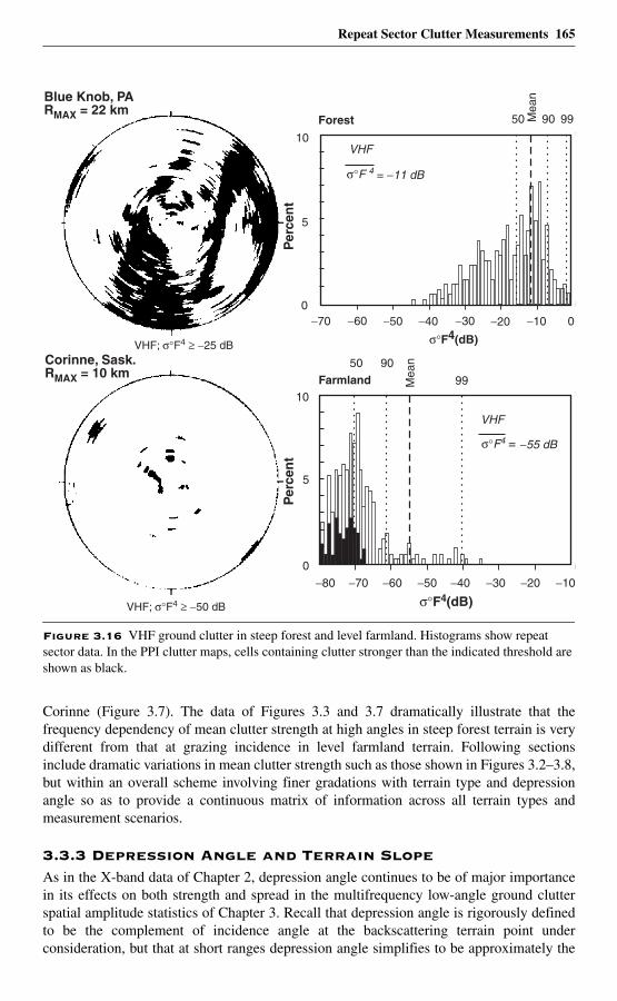
Repeat Sector Clutter Measurements 165

Corinne (Figure 3.7). The data of Figures 3.3 and 3.7 dramatically illustrate that thefrequency dependency of mean clutter strength at high angles in steep forest terrain is verydifferent from that at grazing incidence in level farmland terrain. Following sectionsinclude dramatic variations in mean clutter strength such as those shown in Figures 3.2–3.8,but within an overall scheme involving finer gradations with terrain type and depressionangle so as to provide a continuous matrix of information across all terrain types andmeasurement scenarios.

3.3.3 Depression Angle and Terrain SlopeAs in the X-band data of Chapter 2, depression angle continues to be of major importancein its effects on both strength and spread in the multifrequency low-angle ground clutterspatial amplitude statistics of Chapter 3. Recall that depression angle is rigorously definedto be the complement of incidence angle at the backscattering terrain point underconsideration, but that at short ranges depression angle simplifies to be approximately the

Figure 3.16 VHF ground clutter in steep forest and level farmland. Histograms show repeat sector data. In the PPI clutter maps, cells containing clutter stronger than the indicated threshold are shown as black.

Blue Knob, PARMAX = 22 km

Corinne, Sask.RMAX = 10 km

VHF; σ°F4 ≥ −25 dB

VHF; σ°F4 ≥ −50 dB

10

5

0

σ°F4(dB)−80 −70 −60 −50 −40 −30 −10−20

Farmland50 90

99Mea

n

Per

cen

t

5

Per

cen

t

10

0

σ°F4(dB)

−70 −60 −50 −40 −30 −20 0−10

Forest 50 90 99Mea

n

VHF

= −11 dBσ°F 4

=

VHF

σ°F4 −55 dB

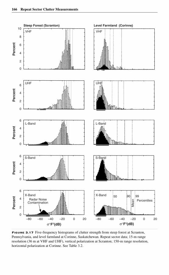
166 Repeat Sector Clutter Measurements

Figure 3.17 Five-frequency histograms of clutter strength from steep forest at Scranton, Pennsylvania, and level farmland at Corinne, Saskatchewan. Repeat sector data; 15-m range resolution (36 m at VHF and UHF), vertical polarization at Scranton; 150-m range resolution, horizontal polarization at Corinne. See Table 3.2.

Steep Forest (Scranton)

Per

cen

t

Level Farmland (Corinne)10

0

2

4

6

8

Per

cen

t

0

2

4

6

Per

cen

t

0

2

4

6

Per

cen

t

0

2

4

6

Per

cen

t

0

2

4

6

L-Band L-Band

UHF UHF

VHF VHF

S-Band S-Band

X-Band X-BandRadar Noise

Contamination

–80 –60 –40 –20 0 20 –80 –60 –40 –20 0 20

σ°F4(dB) σ°F4(dB)

50 90 99Percentiles

Mea

n

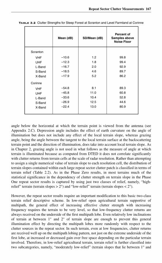
Repeat Sector Clutter Measurements 167

angle below the horizontal at which the terrain point is viewed from the antenna (seeAppendix 2.C). Depression angle includes the effect of earth curvature on the angle ofillumination but does not include any effect of the local terrain slope, whereas grazingangle, being the angle between the tangent to the local terrain surface at the backscatteringterrain point and the direction of illumination, does take into account local terrain slope. Asin Chapter 2, grazing angle is not used in what follows as the measure of angle at whichterrain is illuminated because as computed from DTED it does not correlate significantlywith clutter returns from terrain cells at the scale of radar resolution. Rather than attemptingto assign a single numerical value of terrain slope to each resolution cell, the distribution ofterrain slopes contained within each large repeat sector clutter patch is classified in terms ofterrain relief (Table 2.2). As in the Phase Zero results, in most terrains much of thestatistical significance in the dependency of clutter strength on terrain slope in the PhaseOne repeat sector results is captured by using just two classes of relief, namely, “high-relief” terrain (terrain slopes > 2°) and “low-relief” terrain (terrain slopes < 2°).

However, the repeat sector results require an important modification to this basic two-classterrain relief descriptive scheme. In low-relief open agricultural terrain supportive ofmultipath, the general effect of increasing effective clutter strength with increasingfrequency requires the terrain to be very level, so that low-frequency clutter returns arealways received on the underside of the first multipath lobe. Even relatively low inclinationsof terrain at between 1° and 2° of terrain slope are enough to prevent this generalillumination effect by directing the multipath lobes more randomly with respect to theclutter sources in the repeat sector. In such terrain, even at low frequencies, clutter returnsare received well up on the multipath lobing pattern, not just on the extreme underside of thefirst lobe, at increased or decreased gain over free space depending on the particular terraininvolved. Therefore, in low-relief agricultural terrain, terrain relief is further classified intotwo subcategories, namely, “moderately low-relief” (terrain slopes that lie between 1° and

Table 3.2 Clutter Strengths for Steep Forest at Scranton and Level Farmland at Corinne

Mean (dB) SD/Mean (dB)Percent of

Samples aboveNoise Floor

Scranton

VHF

UHF

L-Band

S-Band

X-Band

Corinne

VHF

UHF

L-Band

S-Band

X-Band

–10.6

–12.3

–16.7

–18.5

–17.9

–54.8

–45.8

–33.6

–26.9

–22.4

1.2

1.8

2.0

4.6

5.2

8.1

11.0

10.4

12.5

13.0

99.8

99.4

92.9

89.7

86.2

89.3

60.8

52.8

44.6

80.9

168 Repeat Sector Clutter Measurements

2°) and “very low-relief” (terrain slopes < 1°). This refinement in classification is sufficientto distinguish between terrain that is level enough so that multipath results in generallyincreasing strength of illumination of clutter sources with increasing frequency, and terrainin which multipath effects on illumination are more specific.

3.4 Mean Land Clutter Strength vs Frequency by Terrain TypeSection 3.4 shows how mean land clutter strength varies with radar frequency as measuredwithin Phase One repeat sectors. These results depend on three different categories ofdescriptive parameter. First, there are parameters descriptive of the radar; namely,frequency, resolution, and polarization. The basic format of data presentation shows meanstrength vs frequency across the five Phase One frequency bands for each of fourcombinations of pulse length and polarization. Second, there are parameters descriptive ofthe geometry of illumination. Depression angle is the parameter used herein, a quantityrelatively simple and unambiguous to determine, depending as it does simply on range andrelative elevation difference (Table 3.1) between the radar antenna and the centroid of therepeat sector clutter patch. Third, there are parameters descriptive of the terrain within therepeat sector clutter patch. The terrain within each repeat sector is classified herein both interms of its land cover (Table 2.1) and its landform (Table 2.2). The terrain classificationswere obtained by overlaying and registering measured clutter maps onto stereo aerialphotos and topographic maps. All of these parameters have been previously introduced.

Table 3.3 describes the repeat sectors at 38 different Phase One measurement sites in termsof range and azimuth extent from the radar, depression angle, and terrain type by landformand land cover in decreasing order by percent area within the repeat sector clutter patch. Itis apparent in Table 3.3 that every repeat sector is different (terrain is essentially infinitelyvariable). As a result of this variability, the set of 20 multifrequency repeat sector meanclutter strengths is different, at least in detail, for every site. The current objective is tomove beyond this abundance of detail to determine useful simple generalizations in themeasurement results. The approach taken here to achieve this objective requires thestatistical combination of measurements that are reasonably similar within broad classes ofterrain type and depression angle, such that the results satisfactorily cluster within eachclass and significantly separate between different classes.

The repeat sectors in Table 3.3 are grouped within the best such broad classes that weredeveloped in the repeat sector database. Five broadly different terrain classes are defined inTable 3.3, namely, (1) urban, (2) mountains, (3) forest, (4) agricultural, and (5) desert,marsh, or grassland. Except for mountains, these groups are basically distinguished bymajor land cover type; mountains are distinguished more by landform. Within each class,when terrain relief can vary enough within class to require further subclassification, twosubcategories of terrain relief are usually enough, low-relief with terrain slopes < 2°, andhigh-relief with terrain slopes > 2°. An exception is agricultural terrain, which requiresadditional subclassification of low-relief terrain into categories of moderately low-reliefwith terrain slopes between 1° and 2°, and very low-relief with terrain slopes < 1°. For eachterrain type/relief category, when depression angle can vary enough within class to beimportant, usually three categories of depression angle (low, intermediate, and high) areenough to separate effects.

4Approaches to Clutter

Modeling

4.1 IntroductionThe historical technical literature on low-angle land clutter includes a number of differentpast approaches for attempting to model this complex phenomenon, as reviewed inChapter 1. Thus, most simply, low-angle clutter has been characterized as a single-variablecharacteristic or functional relationship between the dependent variable σ ° and any one ofthe following three independent variables: (1) illumination angle to the backscatteringterrain point; (2) radar carrier frequency; and (3) range to the backscattering terrain point.Chapters 2 and 3 illustrate at some length the strong dependencies of low-angle clutter onillumination (i.e., depression) angle and radar carrier frequency based on Phase Zero X-band data and Phase One five-frequency repeat sector data, respectively.

Although providing new useful clutter modeling information, the results of Chapters 2 and3 in themselves do not constitute a clutter model generalized to be applicable to anysurface-sited radar. The objective of such a model is to provide a description of theamplitude statistics of the clutter returns received by an arbitrary radar in a specifiedenvironment. As has been discussed previously in this book, the mean strength (firstmoment) of the clutter amplitude distribution depends strongly on (1) depression angle and(2) radar frequency. However, the equally important shape parameter (derived from theratio of second to first moments) of the clutter amplitude distribution is fundamentallydependent on the spatial resolution of the radar. The modeling information of Chapters 2and 3 is restricted to Phase Zero and Phase One pulse lengths and beamwidths. As such,this modeling information may be used to replicate clutter in radars of Phase Zero or PhaseOne spatial resolution, but is not generalized there to be applicable to radars of spatialresolution significantly different from the Phase Zero and Phase One radars.

Chapter 4 provides an interim angle-specific clutter model fully generalized to beapplicable to radars of arbitrary spatial resolution. This interim model is presented inSection 4.2. It is based on the Phase Zero X-band database (Chapter 2) and the Phase Onerepeat sector database (Chapter 3) and includes all important trends of variation of low-angle clutter amplitude statistics seen in these two databases, including the generaldependency of shape parameter on the spatial resolution or cell size of the radar. Theinterim clutter model is thus a complete model applicable to any surface-sited radar in anyground environment. This model is labelled “interim” because it does not have thestatistical depth of the spatially comprehensive 360° Phase One survey data. The identical

286 Approaches to Clutter Modeling

structure of the interim clutter model carries forward to the more comprehensive modelinginformation of Chapter 5 which is based on the Phase One survey data.

The presentation of material in Chapter 4 is as follows. First, Section 4.1.1 describes animportant clutter modeling objective, namely, the prediction or simulation of plan-positionindicator (PPI) clutter maps in surface-sited radars. Then Section 4.1.2 discusses the cluttermodeling rationale of this book, distinguishing between angle-specific clutter modelinginformation suitable for site-specific clutter prediction using digitized terrain elevation data(DTED) and non-angle-specific modeling information suitable for more generic clutterprediction. Section 4.1.3 discusses clutter as a statistical random process and brieflydescribes the scope of included material within the context of available random-processstatistical attributes. Section 4.2 presents the angle-specific interim clutter model, whichrequires specification of the depression angle to each clutter patch. This model explicitlyincorporates the interdependent effects on clutter of (1) depression angle and (2) radarfrequency, but the effects of (3) range occur implicitly in its site-specific applicationwhereby the occurrences of visible clutter patches decrease with increasing range at eachspecific site.

PPI clutter maps in surface-sited radars are inherently patchy in character. The details of thepatchiness are specific to each site. There remains a need, however, for a generic non-site-specific approach to clutter modeling in which the spatial character of the clutter field is notpatchy. An important feature of a PPI clutter map for a surface-sited radar, disregarding thespecificities of patchiness in each such map, is the obvious dissipation of the clutter withincreasing range. Section 4.3 takes up the subject of non-angle-specific clutter modelinginformation suitable for use in non-patchy prediction. This naturally leads to the explicitintroduction of (3) range as the important independent variable affecting the clutter, incontrast to effects of range occurring implicitly in site-specific modeling. What becomesapparent based on clutter measurements at many sites is that the occurrence of clutterfundamentally depends upon (i.e., decreases with) range, for a given site height; and thatthe strength of the clutter where it occurs is fundamentally dependent upon terrain type butnot upon range. Section 4.3 provides a simple, generic, non-patchy clutter model basedupon these observations in the measurement data.

Section 4.4 discusses the intimate interrelationship at low angles between geometricallyvisible terrain and clutter occurrence. Section 4.5 discusses the difficulties involved at lowangles in attempting to distinguish discrete from distributed clutter and takes up the issue ofhow best to reduce the measurement data. Section 4.6 provides additional insight into theclutter phenomenon and the ramifications in its modeling by providing brief introductorydiscussions of its temporal statistics, its spectral characteristics, and its correlativeproperties. Section 4.7 summarizes many of the insights developed in Chapter 4.Appendices 4.A, 4.B, and 4.C further develop the effects of radar height and range in low-angle clutter and discuss the complications introduced by range-dependent sensitivitylimitations and the corresponding range-dependent effects of radar noise corruption inclutter measurement data. Appendix 4.D describes a more computationally intensiveapproach to low-angle clutter modeling in which spatial cells that are locally strong (i.e.,“discretes”) compared to their neighbors are modeled separately from the weakerneighboring (i.e., “background”) cells.

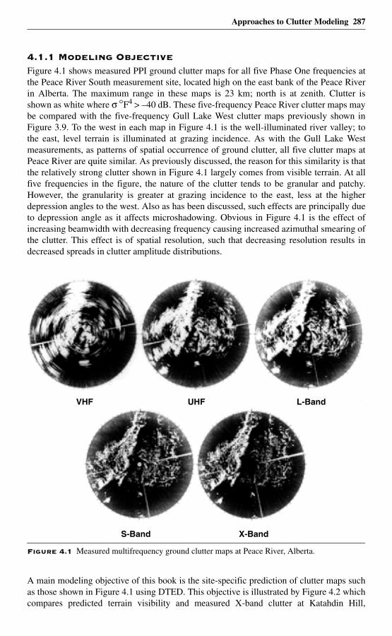
Approaches to Clutter Modeling 287

4.1.1 Modeling ObjectiveFigure 4.1 shows measured PPI ground clutter maps for all five Phase One frequencies atthe Peace River South measurement site, located high on the east bank of the Peace Riverin Alberta. The maximum range in these maps is 23 km; north is at zenith. Clutter isshown as white where σ °F4 > –40 dB. These five-frequency Peace River clutter maps maybe compared with the five-frequency Gull Lake West clutter maps previously shown inFigure 3.9. To the west in each map in Figure 4.1 is the well-illuminated river valley; tothe east, level terrain is illuminated at grazing incidence. As with the Gull Lake Westmeasurements, as patterns of spatial occurrence of ground clutter, all five clutter maps atPeace River are quite similar. As previously discussed, the reason for this similarity is thatthe relatively strong clutter shown in Figure 4.1 largely comes from visible terrain. At allfive frequencies in the figure, the nature of the clutter tends to be granular and patchy.However, the granularity is greater at grazing incidence to the east, less at the higherdepression angles to the west. Also as has been discussed, such effects are principally dueto depression angle as it affects microshadowing. Obvious in Figure 4.1 is the effect ofincreasing beamwidth with decreasing frequency causing increased azimuthal smearing ofthe clutter. This effect is of spatial resolution, such that decreasing resolution results indecreased spreads in clutter amplitude distributions.

A main modeling objective of this book is the site-specific prediction of clutter maps suchas those shown in Figure 4.1 using DTED. This objective is illustrated by Figure 4.2 whichcompares predicted terrain visibility and measured X-band clutter at Katahdin Hill,

Figure 4.1 Measured multifrequency ground clutter maps at Peace River, Alberta.

VHF UHF L-Band

S-Band X-Band

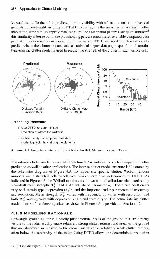
288 Approaches to Clutter Modeling

Massachusetts. To the left is predicted terrain visibility with a 5-m antenna on the basis ofgeometric line-of-sight visibility in DTED. To the right is the measured Phase Zero cluttermap at the same site. In approximate measure, the two spatial patterns are quite similar;24

this similarity is borne out in the plot showing percent circumference visible compared withpercent circumference in measured clutter vs range. DTED are used to deterministicallypredict where the clutter occurs, and a statistical depression-angle-specific and terrain-type-specific clutter model is used to predict the strength of the clutter in each visible cell.

The interim clutter model presented in Section 4.2 is suitable for such site-specific clutterprediction as well as other applications. The interim clutter model structure is illustrated bythe schematic diagram of Figure 4.3. To model site-specific clutter, Weibull randomnumbers are distributed cell-by-cell over visible terrain as determined by DTED. Asindicated in Figure 4.3, the Weibull numbers are drawn from distributions characterized bya Weibull mean strength and a Weibull shape parameter aw. These two coefficientsvary with terrain type, depression angle, and the important radar parameters of frequencyand resolution. Mean strength varies with frequency, aw varies with resolution, andboth and aw vary with depression angle and terrain type. The actual interim cluttermodel matrix of numbers organized as shown in Figure 4.3 is provided in Section 4.2.

4.1.2 Modeling RationaleLow-angle ground clutter is a patchy phenomenon. Areas of the ground that are directlyvisible to the radar usually cause relatively strong clutter returns, and areas of the groundthat are shadowed or masked to the radar usually cause relatively weak clutter returns,often below the sensitivity of the radar. Using DTED allows the deterministic prediction

24. But see also Figure 2.11, a similar comparison at finer resolution.

Figure 4.2 Predicted clutter visibility at Katahdin Hill. Maximum range = 35 km.

Predicted Measured

Digitized TerrainElevation Data

X-Band Clutter Mapσ° > –40 dB

Per

cen

t C

ircu

mfe

ren

ce V

isib

le

1) Use DTED for deterministictatistical prediction of where the clutter is

2) Subsequently use empirical statistical model to predict how strong the clutter is

Modeling Procedure

100

30

10

3

1.0

0.3

Range (km)

0 10 20 30 40

Measured

Predicted

σ °w

σ °wσ °w

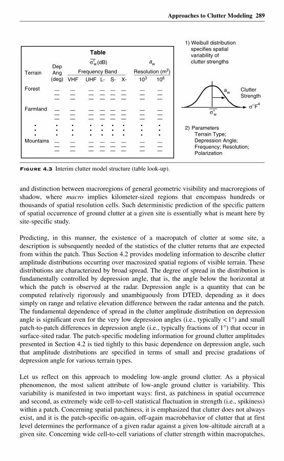
Approaches to Clutter Modeling 289

and distinction between macroregions of general geometric visibility and macroregions ofshadow, where macro implies kilometer-sized regions that encompass hundreds orthousands of spatial resolution cells. Such deterministic prediction of the specific patternof spatial occurrence of ground clutter at a given site is essentially what is meant here bysite-specific study.

Predicting, in this manner, the existence of a macropatch of clutter at some site, adescription is subsequently needed of the statistics of the clutter returns that are expectedfrom within the patch. Thus Section 4.2 provides modeling information to describe clutteramplitude distributions occurring over macrosized spatial regions of visible terrain. Thesedistributions are characterized by broad spread. The degree of spread in the distribution isfundamentally controlled by depression angle, that is, the angle below the horizontal atwhich the patch is observed at the radar. Depression angle is a quantity that can becomputed relatively rigorously and unambiguously from DTED, depending as it doessimply on range and relative elevation difference between the radar antenna and the patch.The fundamental dependence of spread in the clutter amplitude distribution on depressionangle is significant even for the very low depression angles (i.e., typically < 1°) and smallpatch-to-patch differences in depression angle (i.e., typically fractions of 1°) that occur insurface-sited radar. The patch-specific modeling information for ground clutter amplitudespresented in Section 4.2 is tied tightly to this basic dependence on depression angle, suchthat amplitude distributions are specified in terms of small and precise gradations ofdepression angle for various terrain types.

Let us reflect on this approach to modeling low-angle ground clutter. As a physicalphenomenon, the most salient attribute of low-angle ground clutter is variability. Thisvariability is manifested in two important ways: first, as patchiness in spatial occurrenceand second, as extremely wide cell-to-cell statistical fluctuation in strength (i.e., spikiness)within a patch. Concerning spatial patchiness, it is emphasized that clutter does not alwaysexist, and it is the patch-specific on-again, off-again macrobehavior of clutter that at firstlevel determines the performance of a given radar against a given low-altitude aircraft at agiven site. Concerning wide cell-to-cell variations of clutter strength within macropatches,

Figure 4.3 Interim clutter model structure (table look-up).

Table

Terrain

Forest

Farmland

Mountains

DepAng(deg)

Frequency Band

VHF UHF L- S- X-

———

———

———

———

———

———

———

———

———

———

———

———

———

———

———

———

———

———

103 106

Resolution (m2)

———

———

———

———

———

———

(dB)

1) Weibull distribution specifies spatial variability of clutter strengths

ClutterStrength

F4

2) Parameters Terrain Type; Depression Angle; Frequency; Resolution; Polarization

aww

aw

w

•••

•••

•••

•••

•••

•••

•••

•••

•••

290 Approaches to Clutter Modeling

it is emphasized that what appears at first consideration to be a phenomenon of extremevariability and little predictability turns out in the end, after much data analysis, to begenerally dependent on very fine differences in depression angle.

Use of site-specific DTED allows the capture of both these basic attributes of low-angleground clutter, its spatial patchiness (approximately computed simply as geometricvisibility), and (through depression angle) its expected range of amplitudes within a patch.Therefore, this approach to modeling low-angle clutter is regarded as a major advance overmore general non-patchy approaches that do not distinguish between macroregions ofclutter occurrence and macroregions of shadow. This approach allows an analyst to predict,within macroregions, where a surface-sited radar can be expected to encounter clutterinterference and where the radar will be free of such interference; and, given that the radaris experiencing clutter, what, on the average, the expected statistics of signal-to-clutter ratiowill be across the macroregion of clutter.

Clutter returns within patches are often highly spatially correlated. This book discusses thefact that the dominant clutter sources within macroregions of general geometric visibilityare usually spatially localized or discrete, such that groups of cells providing strong returnsare often separated by cells providing weak or noise-level returns. The occurrence of noise-level returns distributed within macroregions of general geometric visibility is referred to as“microshadowing,” where micro implies resolution-cell-sized areas (see Figure 2.11 and itsaccompanying discussion in Chapter 2). The high degree of spatial microcorrelation ofstrong discrete sources within macropatches results from the fact that such sources exist asvertical features of landscape discontinuity that often occur in definite patterns, forexample, along the leading edge of a tree line or the clustering of vertical objects alongroads and field boundaries. If an analyst is interested in the actual microstatistics, forexample, of break-lock in a surface radar tracking a target across a given clutter patch, theinformation in this book does not go that far.

The kind of detail and fidelity in terrain description that are required to predictmicrostatistics of spatial correlation of clutter amplitudes within macropatches are regardedas a second sequential major hurdle to cross in clutter modeling. Limitations encountered inattempting this second advance have been explored. It has been found that prediction ofmicrospatial correlation is a very challenging task that immediately takes exploratoryoperations out to the limits of current resources in terms of available information andcomputer processing. In contrast, the first major advance in low-angle clutter fidelity, whichis the field-of-investigation of this book, comes relatively easily once DTED are in play.

The above allusion to general non-patchy approaches to clutter modeling does not implythat such approaches are without value. Section 4.3 moves from measurements in which thepatch-specific parameter of depression angle is the fundamental controlling parameter tonon-angle-specific modeling information based on relatively general parameters such assite height, terrain roughness, and terrain type (e.g., forest, agricultural, etc.). However, it istrue that non-patchy approaches to clutter modeling are, indeed, relatively abstract andconceptually vague in quantitative study. This is the logical penalty that non-patchyapproaches must pay as the price for generality. This penalty comes about because, insteadof aggregating system performance measures after realistic clutter computations at manyindividual sites, the non-patchy approach attempts to aggregate and generalize clutterinfluences before a one-time assessment of system performance. That is, the non-patchy

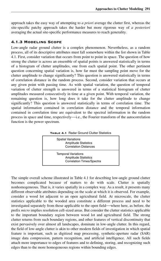
Approaches to Clutter Modeling 291

approach takes the easy way of attempting to a priori average the clutter first, whereas thesite-specific patchy approach takes the harder but more rigorous way of a posterioriaveraging the actual site-specific performance measures to reach generality.

4.1.3 Modeling ScopeLow-angle radar ground clutter is a complex phenomenon. Nevertheless, as a randomprocess, all of its descriptive attributes must fall somewhere within the list shown in Table4.1. First, consider variation that occurs from point to point in space. The question of howstrong the clutter is across an ensemble of spatial points is answered statistically in termsof a histogram of clutter amplitudes, one from each spatial point. The other pertinentquestion concerning spatial variation is, how far must the sampling point move for theclutter amplitude to change significantly? This question is answered statistically in termsof correlation distance in the random process. Second, consider variation that occurs atany given point with passing time. As with spatial variation, the question of temporalvariation of clutter strength is answered in terms of a statistical histogram of clutteramplitudes measured consecutively in time at a given point. With temporal variation, theremaining question is, how long does it take for the clutter amplitude to changesignificantly? This question is answered statistically in terms of correlation time. Thespatial information contained in correlation distance and the temporal informationcontained in correlation time are equivalent to the spectral information in the randomprocess in space and time, respectively—i.e., the Fourier transform of the autocorrelationfunction is the power spectrum.

The simple overall scheme illustrated in Table 4.1 for describing low-angle ground clutterbecomes complicated because of matters to do with scale. Clutter is spatiallynonhomogeneous. That is, it varies spatially in a complex way. As a result, it presents manydifferent observable attributes depending on the scale at which it is observed. For example,consider a wood lot adjacent to an open agricultural field. At microscale, the clutterstatistics applicable to the wooded area constitute a different process and need to beinvestigated separately from those applicable to the open field—where here, as before, theprefix micro implies resolution cell-sized areas. But consider the clutter statistics applicableto the important boundary region between wood lot and agricultural field. The strongclutter returns from such boundary regions, and other features of vertical discontinuity thatexist pervasively over almost all landscapes, dominate in low-angle clutter. In this regard,the field of low-angle clutter is akin to other modern fields of investigation in which spatialfeature is important, such as digitized map processing, synthetic-aperture radar (SAR)image data compression, pattern recognition, and artificial intelligence. All such fieldsattach more importance to edges of features and to defining, storing, and recognizing suchedges than to the more homogeneous regions within bounding edges.

Table 4.1 Radar Ground Clutter Statistics

Spatial Variations Amplitude Statistics Correlation Distances

Temporal Variations Amplitude Statistics Correlation Times/Spectra

292 Approaches to Clutter Modeling

Thus, the field of low-angle clutter leads an investigator from microscale to macroscale,where here, also as before, the prefix macro implies kilometer-sized regions encompassinghundreds or thousands of spatial resolution cells and many vertical features. As discussedin Chapter 2, the correct empirical approach in dealing with many edges of featuresexisting as discontinuous or discrete clutter sources is to collect meaningful numbers ofthem together within macropatches, allowing the terrain classification system to describetheir statistical attributes at an overall level of description. This book provides modelinginformation allowing the prediction of the spatial amplitude statistics of low-angle clutteras they occur for ground-based radar distributed over macroregions of visible terrain.Development of this information requires clutter measurements from many different sitesand macropatches to build up an appropriate supportive empirical statistical database. Thisbook does not address statistical issues of patch length and separation, but Chapter 4 and itsappendices address how, as a result of spatial patchiness, the occurrence of clutter generallydecreases with increasing range. An example showing microscale correlation distance infarmland terrain is provided in Section 4.6. Such microspatial correlation is important, forexample, in the detailed processing algorithms of constant-false-alarm rate (CFAR) radars.

Issues of temporal variation of low-angle ground clutter generally stand apart from themore stressing problem of modeling the spatial statistics of clutter. The subjects overlapsomewhat in that clutter spatial amplitude statistics vary with long-term temporal variationassociated with weather and season. Long-term temporal variation is discussed in Chapter3. Concerning short-term temporal variation, some brief information describing the relativefrequency of occurrence of temporal amplitude statistics between cells with Rayleigh (i.e.,windblown foliage) and Ricean (i.e., fixed discretes embedded in foliage) statistics isprovided in Section 4.6. Section 4.6 also introduces the subject of intrinsic-motion Dopplerfrequency spectra of windblown ground clutter; the accurate characterization of windblownclutter spectra is more extensively addressed as the subject of Chapter 6.

4.2 An Interim Angle-Specific Clutter Model

4.2.1 Model BasisSection 4.2 presents an interim angle-specific clutter model for predicting ground clutteramplitude statistics as they occur over spatial macroregions of directly visible terrain at lowdepression angles. The interim clutter model is based upon Phase Zero X-band and PhaseOne five-frequency measurements as discussed in Chapters 2 and 3, respectively. The resultsof Chapters 2 and 3 apply specifically to cell sizes as defined by Phase Zero and Phase Onepulse lengths and beamwidths. The interim model generalizes these results such that thespatial resolution of the radar becomes an important—and, within limits, arbitrarilyspecifiable—independent variable upon which the clutter statistics strongly depend.

The spread in the clutter amplitude distribution as defined by the shape parameter of thedistribution is fundamentally dependent on the spatial resolution of the radar. Spatialresolution or cell size A in m2 is defined by A = r·∆r·∆θ where r is range, ∆r is rangeresolution, and ∆θ is beamwidth (see Section 2.3.1.1). The range of cell sizes empiricallyavailable in the Phase Zero and Phase One data is determined not only by the differentpulse lengths provided by the Phase Zero and Phase One radars (viz., 0.06, 0.1, 0.25, 0.5,and 1.0 µs), but also and very importantly by the different azimuth beamwidths available(viz., 1°, 3°, 5°, 13°) and by the different ranges over which clutter patch amplitude

Approaches to Clutter Modeling 293

distributions were acquired (viz., from 1 to > 50 km). Of course, each azimuth beamwidthis generally available in only one radar frequency band in the clutter measurement data, butit turns out that the spread in the clutter amplitude distribution, determined, for example, bythe ratio of standard deviation-to-mean, is relatively independent of the radar frequency atwhich it is measured. The spatial spikiness causing spread in low-angle clutter—acharacteristic feature easily observed in A-scope sector displays—is relatively independentof radar frequency because the same large discrete sources causing the spikes existwhatever the frequency band employed in the measurement.

Therefore, observed spreads in clutter amplitude distributions, which are fundamentallyand strongly dependent on cell size, may be considered as independent of frequency andthus may be combined and interpolated across the beamwidths available in the variousfrequency bands to provide a much wider range of spatial resolution than would beavailable in any one frequency band alone. By this means, the interim clutter model, andalso the clutter modeling information provided subsequently in Chapter 5, are generalizedsuch that the highly significant spreads in clutter amplitude distributions apply to radar cellsizes ranging over the relatively wide extent from ~103 m2 to ~106 m2 in any frequencyband. This matter is further discussed in Chapter 5.

The Phase Zero X-band results of Chapter 2 underlying the interim clutter model comprisemeasurements from 2,177 different clutter patches. With this large number of terrainsamples, even after separating into different categories of terrain type and depression angle,there are still many samples left in any given category and hence good statistical definitionin the results. That is, with a large amount of averaging at work in these data, even smalldifferences in results are statistically significant. In contrast, the Phase One five-frequencyresults of Chapter 3 underlying the interim clutter model comprise measurements from just42 repeat sector terrain patches, one per site from each of the 42 Phase One sites. Becausebackscatter measurements were performed on each repeat sector patch a number of timesacross a 20-element radar parameter matrix, the Phase One repeat sector database of Chapter3 constitutes a comparable amount of data to the Phase Zero database and alloweddetermination of trends of variation with frequency, pulse length and polarization. It isimportant to realize, however, that when looking for such trends and separating the 42 repeatsector patches into various categories of terrain type and depression angle, in contrast toPhase Zero there often are not very many terrain samples per category. As a result, theinterim clutter model reaches for multifrequency characteristics often on the basis of a fewexamples of an observed trend rather than with the statistical rigor of Phase Zero.

This lack of statistical depth in the interim clutter model is evidenced by the fact that theinterim model is presented as a simple one-page table of numbers. There are obviousadvantages to this simplicity, both in ease of comprehension and ease of implementation.As a result of such advantages, the interim clutter model has received and continues toreceive extensive usage at Lincoln Laboratory and elsewhere. The disadvantages of thissimplicity are less statistical rigor and diminished prediction accuracy. Chapter 5 brings allthe Phase One 360º survey data at each site under analysis, in addition to the repeat sectordata, utilizing the same model construct as employed by the interim clutter model. In doingso, the Phase One modeling information of Chapter 5 obtains the important Phase Zerostatistical advantage of many terrain samples and increased prediction accuracy.

294 Approaches to Clutter Modeling

4.2.2 Interim ModelThe interim angle-specific clutter model is presented in Table 4.2. The clutter modelinginformation in Table 4.2 is provided within a context of Weibull statistics [1, 2], where

is the Weibull mean strength and aw is the Weibull shape parameter. Weibull statisticsare defined and discussed in Appendices 2.B and 5.A. The interim model is based uponthe three main categories of descriptive parameter of low-angle clutter previouslyintroduced in Section 3.4. First are parameters which are descriptive of the radar. Theimportant radar parameters affecting clutter statistics as employed in the interim model areradar frequency as it affects and radar spatial resolution as it affects aw.

Second are parameters descriptive of the geometry of illumination of the clutter patch. Asin Chapters 2 and 3, the interim model utilizes depression angle, a relatively simple andunambiguous quantity to determine, depending only on range and relative elevationdifference between the radar antenna and the backscattering terrain point. Recall thatattempts in Chapter 2 to use grazing angle met with little additional success, partly due todifficulties associated with scale, precision, and accuracy in unambiguously defining localterrain slope and partly because dominant clutter sources tend to be vertical discrete objectsassociated with the land cover. Use of grazing angle in clutter modeling is further discussedin Appendix 4.D. Formulating the interim clutter model in terms of depression angleinvolves the possibility of occurrence of negative depression angles wherein terrain isobserved by the radar at elevations above the antenna. For terrain to be visible at negativedepression angle requires the terrain to be of terrain slope greater than the absolute value ofthe depression angle at which it is observed.

Third are parameters descriptive of the terrain within the clutter patch. The interim cluttermodel of Table 4.2 is comprehensive in that, whatever terrain is under consideration, itmust fall within one of the terrain types of the model. Most terrain types in the modelinvolve several depression angle regimes. As introduced in Chapter 2, the important generalterrain types of the interim model are threefold, namely (1) rural/low-relief terrain in whichterrain slopes are < 2°; (2) rural/high-relief terrain in which terrain slopes are > 2°; and (3)urban terrain.

Within general rural/low-relief terrain, the interim model further distinguishes threespecific important subclass terrain types as discussed in Chapter 3, namely, continuousforest, open farmland, and open wasteland (e.g., desert, marsh) or grazing land with verylow incidence of large discrete vertical objects (e.g., farmstead buildings, feed storage silos,isolated trees, etc.) such as typically occur in farmland. Within rural/high-relief terrain,particularly separated out are the two subclass terrain types of continuous forest andmountains. Within urban terrain, separated out is the subclass of urban areas as observedover open low-relief terrain supportive of multipath (see Chapter 3). Concerning the severalsubcategories of terrain contained within each of the three general terrain types in Table4.2, the general category (a) is applicable only if the terrain in question fails to meet thespecification of any of the subsequent specific subcategories within a group. That is, thegeneral category applies to mixed or composite terrain that is neither completely open norcompletely tree-covered. The subcategorization of terrain within each major groupbecomes increasingly important with decreasing frequency. For completeness, a fourthgeneral category comprising terrain observed at negative depression angle is required.Terrain observed at negative depression angle is usually relatively steep.

σ °w

σ °w

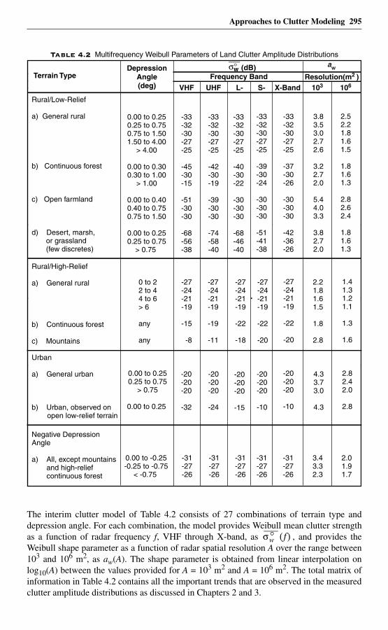
Approaches to Clutter Modeling 295

The interim clutter model of Table 4.2 consists of 27 combinations of terrain type anddepression angle. For each combination, the model provides Weibull mean clutter strengthas a function of radar frequency f, VHF through X-band, as , and provides theWeibull shape parameter as a function of radar spatial resolution A over the range between103 and 106 m2, as aw(A). The shape parameter is obtained from linear interpolation onlog10(A) between the values provided for A = 103 m2 and A = 106 m2. The total matrix ofinformation in Table 4.2 contains all the important trends that are observed in the measuredclutter amplitude distributions as discussed in Chapters 2 and 3.

Table 4.2 Multifrequency Weibull Parameters of Land Clutter Amplitude Distributions

Urban

a) General urban

b) Urban, observed on open low-relief terrain

0.00 to 0.250.25 to 0.75

> 0.75

0.00 to 0.25

-20-20-20

-32

-20-20-20

-24

-20-20-20

-15

-20-20-20

-10

-20-20-20

-10

4.33.73.0

4.3

2.82.42.0

2.8

Rural/High-Relief

a) General rural

b) Continuous forest

c) Mountains

0 to 22 to 44 to 6> 6

any

any

-27-24-21-19

-15

-8

-27-24-21-19

-19

-11

-27-24-21-19

-22

-18

-27-24-21-19

-22

-20

-27-24-21-19

-22

-20

2.21.81.61.5

1.8

2.8

1.41.31.21.1

1.3

1.6

Rural/Low-Relief

a) General rural

b) Continuous forest

c) Open farmland

d) Desert, marsh, or grassland (few discretes)

0.00 to 0.250.25 to 0.750.75 to 1.501.50 to 4.00

> 4.00

0.00 to 0.300.30 to 1.00

> 1.00

0.00 to 0.400.40 to 0.750.75 to 1.50

0.00 to 0.250.25 to 0.75

> 0.75

-33-32-30-27-25

-45-30-15

-51-30-30

-68-56-38

-33-32-30-27-25

-42-30-19

-39-30-30

-74-58-40

-33-32-30-27-25

-40-30-22

-30-30-30

-68-46-40

-33-32-30-27-25

-39-30-24

-30-30-30

-51-41-38

-33-32-30-27-25

-37-30-26

-30-30-30

-42-36-26

3.83.53.02.72.6

3.22.72.0

5.44.03.3

3.82.72.0

2.52.21.81.61.5

1.81.61.3

2.82.62.4

1.81.61.3

(dB)Frequency Band Resolution(m2 )Terrain Type

DepressionAngle(deg) VHF UHF L- S- X-Band 103 106

Negative DepressionAngle

a) All, except mountains and high-relief continuous forest

0.00 to -0.25-0.25 to -0.75

< -0.75

-31-27-26

-31-27-26

-31-27-26

-31-27-26

-31-27-26

3.43.32.3

2.01.91.7

°σw aw

σ °w f( )

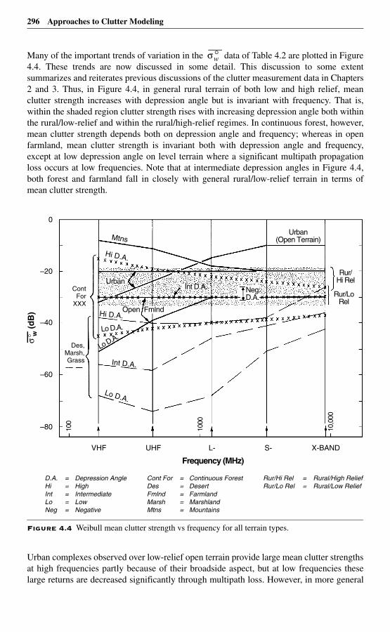
296 Approaches to Clutter Modeling

Many of the important trends of variation in the data of Table 4.2 are plotted in Figure4.4. These trends are now discussed in some detail. This discussion to some extentsummarizes and reiterates previous discussions of the clutter measurement data in Chapters2 and 3. Thus, in Figure 4.4, in general rural terrain of both low and high relief, meanclutter strength increases with depression angle but is invariant with frequency. That is,within the shaded region clutter strength rises with increasing depression angle both withinthe rural/low-relief and within the rural/high-relief regimes. In continuous forest, however,mean clutter strength depends both on depression angle and frequency; whereas in openfarmland, mean clutter strength is invariant both with depression angle and frequency,except at low depression angle on level terrain where a significant multipath propagationloss occurs at low frequencies. Note that at intermediate depression angles in Figure 4.4,both forest and farmland fall in closely with general rural/low-relief terrain in terms ofmean clutter strength.

Urban complexes observed over low-relief open terrain provide large mean clutter strengthsat high frequencies partly because of their broadside aspect, but at low frequencies theselarge returns are decreased significantly through multipath loss. However, in more general

Figure 4.4 Weibull mean clutter strength vs frequency for all terrain types.

σ °w

0

–40

ContFor

XXX

UrbanInt D.A.

Urban(Open Terrain)

Rur/Hi Rel

Rur/LoRel

Neg.D.A.

Des,Marsh,Grass

D.A. = Depression AngleHi = HighInt = IntermediateLo = LowNeg = Negative

Cont For = Continuous ForestDes = DesertFmlnd = FarmlandMarsh = MarshlandMtns = Mountains

Rur/Hi Rel = Rural/High ReliefRur/Lo Rel = Rural/Low Relief

Int D.A.

Lo D.A.Lo D.A.

Hi D.A.

Mtns

Hi D.A.

Lo D.A.

–60

VHF UHF L- S- X-BAND

–80

–20

1000

Frequency (MHz)

100

10,0

00

σ w

(d

B)

°

Open Fmlnd

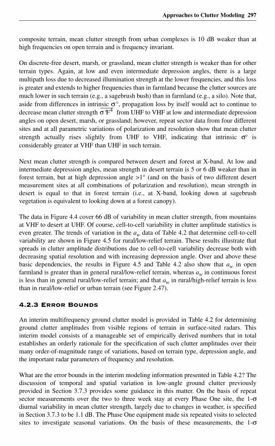
Approaches to Clutter Modeling 297

composite terrain, mean clutter strength from urban complexes is 10 dB weaker than athigh frequencies on open terrain and is frequency invariant.

On discrete-free desert, marsh, or grassland, mean clutter strength is weaker than for otherterrain types. Again, at low and even intermediate depression angles, there is a largemultipath loss due to decreased illumination strength at the lower frequencies, and this lossis greater and extends to higher frequencies than in farmland because the clutter sources aremuch lower in such terrain (e.g., a sagebrush bush) than in farmland (e.g., a silo). Note that,aside from differences in intrinsic σ°, propagation loss by itself would act to continue todecrease mean clutter strength from UHF to VHF at low and intermediate depressionangles on open desert, marsh, or grassland; however, repeat sector data from four differentsites and at all parametric variations of polarization and resolution show that mean clutterstrength actually rises slightly from UHF to VHF, indicating that intrinsic σ° isconsiderably greater at VHF than UHF in such terrain.

Next mean clutter strength is compared between desert and forest at X-band. At low andintermediate depression angles, mean strength in desert terrain is 5 or 6 dB weaker than inforest terrain, but at high depression angle >1° (and on the basis of two different desertmeasurement sites at all combinations of polarization and resolution), mean strength indesert is equal to that in forest terrain (i.e., at X-band, looking down at sagebrushvegetation is equivalent to looking down at a forest canopy).

The data in Figure 4.4 cover 66 dB of variability in mean clutter strength, from mountainsat VHF to desert at UHF. Of course, cell-to-cell variability in clutter amplitude statistics iseven greater. The trends of variation in the aw data of Table 4.2 that determine cell-to-cellvariability are shown in Figure 4.5 for rural/low-relief terrain. These results illustrate thatspreads in clutter amplitude distributions due to cell-to-cell variability decrease both withdecreasing spatial resolution and with increasing depression angle. Over and above thesebasic dependencies, the results in Figure 4.5 and Table 4.2 also show that aw in openfarmland is greater than in general rural/low-relief terrain, whereas aw in continuous forestis less than in general rural/low-relief terrain; and that aw in rural/high-relief terrain is lessthan in rural/low-relief or urban terrain (see Figure 2.47).

4.2.3 Error Bounds

An interim multifrequency ground clutter model is provided in Table 4.2 for determiningground clutter amplitudes from visible regions of terrain in surface-sited radars. Thisinterim model consists of a manageable set of empirically derived numbers that in totalestablishes an orderly rationale for the specification of such clutter amplitudes over theirmany order-of-magnitude range of variations, based on terrain type, depression angle, andthe important radar parameters of frequency and resolution.

What are the error bounds in the interim modeling information presented in Table 4.2? Thediscussion of temporal and spatial variation in low-angle ground clutter previouslyprovided in Section 3.7.3 provides some guidance in this matter. On the basis of repeatsector measurements over the two to three week stay at every Phase One site, the 1-σdiurnal variability in mean clutter strength, largely due to changes in weather, is specifiedin Section 3.7.3 to be 1.1 dB. The Phase One equipment made six repeated visits to selectedsites to investigate seasonal variations. On the basis of these measurements, the 1-σ

σ °F4

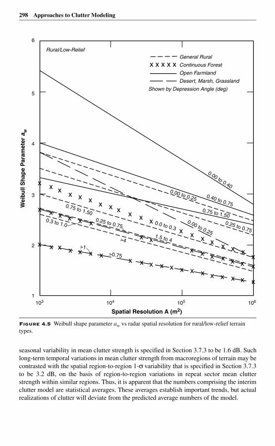
298 Approaches to Clutter Modeling

seasonal variability in mean clutter strength is specified in Section 3.7.3 to be 1.6 dB. Suchlong-term temporal variations in mean clutter strength from macroregions of terrain may becontrasted with the spatial region-to-region 1-σ variability that is specified in Section 3.7.3to be 3.2 dB, on the basis of region-to-region variations in repeat sector mean clutterstrength within similar regions. Thus, it is apparent that the numbers comprising the interimclutter model are statistical averages. These averages establish important trends, but actualrealizations of clutter will deviate from the predicted average numbers of the model.

Figure 4.5 Weibull shape parameter aw vs radar spatial resolution for rural/low-relief terrain types.

x x x x x x x x x

x x x x x

x x x

xxx x x x x

xx

xxxxxxxxxxxxxxxxxxxx

x x x x x x

x xx x x x x x

Rural/Low-ReliefGeneral Rural

Continuous Forest

Open Farmland

Desert, Marsh, Grassland

6

5

103 104

Spatial Resolution A (m2)

Wei

bull

Sh

ape

Par

amet

er a

w

105 106

4

3

2

1

0.00 to 0.40

0.40 to 0.75

0.00 to 0.25

0.75 to 1.50

0.75 to 1.50

0.25 to 0.75

0.00 to 0.251.5 to 4

0.0 to 0.3

0.3 to 1.00.25 to 0.75

>4

>0.75

>1

Shown by Depression Angle (deg)

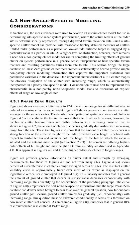
Approaches to Clutter Modeling 299

4.3 Non-Angle-Specific Modeling ConsiderationsIn Section 4.2, the measured data were used to develop an interim clutter model for use indetermining site-specific radar system performance, where the actual terrain at the radarsite is deterministically represented through digitized terrain elevation data. Such a site-specific clutter model can provide, with reasonable fidelity, detailed measures of clutter-limited radar performance as a particular low-altitude airborne target is engaged by aparticular radar at a particular site. At a higher level of abstraction, however, there remainsa need for a non-patchy clutter model for use in computing the limiting effects of groundclutter on system performance in a generic sense, independent of how specific terrainfeatures and resulting patchiness varies from site to site. This section brings the largedatabase of Phase Zero ground clutter measurements statistically to bear to provide simplenon-patchy clutter modeling information that captures the important statistical andparametric variations in the database. One important characteristic of a PPI clutter map isthe obvious dissipation of the clutter with increasing range, which is automaticallyincorporated in a patchy site-specific model. Consideration of how best to implement thischaracteristic in a non-patchy non-site-specific model leads to discussion of expliciteffects of range on low-angle clutter.

4.3.1 Phase Zero ResultsFigure 4.6 shows measured clutter maps to 47-km maximum range for six different sites, inorder of increasing effective radar height. Figure 4.7 shows percent circumference in cluttervs range for the same six sites. The details of each pattern of spatial occurrence of clutter inFigure 4.6 are specific to the terrain features at that site. In all such patterns, however, thepatches of clutter become fewer and farther between with increasing range so that, asshown in Figure 4.7, the amount of clutter that occurs gradually diminishes with increasingrange from the site. These two figures also show that the amount of clutter that occurs is astrong function of the effective height of the radar. Effective radar height is defined withrespect to visible terrain and includes both the height of the hill on which the radar issituated and the antenna mast height (see Section 2.2.3). The somewhat differing higher-order effects of hill height and mast height on terrain visibility are discussed in Appendix4.B. It is apparent in Figures 4.6 and 4.7 that higher radars see clutter to longer ranges.

Figure 4.8 provides general information on clutter extent and strength by averagingmeasurements like those of Figures 4.6 and 4.7 from many sites. Figure 4.8(a) showspercent of circumference in clutter vs range averaged across 86 sites. The resultant cluttervisibility curve is approximately linear over most of its extent as displayed on thelogarithmic vertical scale employed in Figure 4.8(a). This linearity indicates that in generalthe amount of ground clutter that occurs in surface radar decreases exponentially withincreasing range, thus quantifying the observations of the preceding paragraph. The curveof Figure 4.8(a) represents the best non-site-specific information that the large Phase Zerodatabase can deliver when brought to bear to answer the general question, how far out doesground clutter go? Because ground clutter diminishes gradually (i.e., exponentially) withincreasing range, this question must be answered conditionally in terms of a threshold onhow much clutter is of concern. As an example, Figure 4.8(a) indicates that in general 10%of circumference is in clutter at 19-km range.

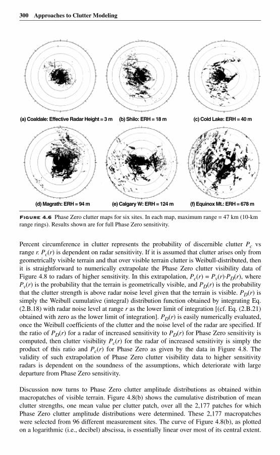
300 Approaches to Clutter Modeling

Percent circumference in clutter represents the probability of discernible clutter Pc vsrange r. Pc(r) is dependent on radar sensitivity. If it is assumed that clutter arises only fromgeometrically visible terrain and that over visible terrain clutter is Weibull-distributed, thenit is straightforward to numerically extrapolate the Phase Zero clutter visibility data ofFigure 4.8 to radars of higher sensitivity. In this extrapolation, Pc(r) = Pv(r)·PD(r), wherePv(r) is the probability that the terrain is geometrically visible, and PD(r) is the probabilitythat the clutter strength is above radar noise level given that the terrain is visible. PD(r) issimply the Weibull cumulative (integral) distribution function obtained by integrating Eq.(2.B.18) with radar noise level at range r as the lower limit of integration [(cf. Eq. (2.B.21)obtained with zero as the lower limit of integration]. PD(r) is easily numerically evaluated,once the Weibull coefficients of the clutter and the noise level of the radar are specified. Ifthe ratio of PD(r) for a radar of increased sensitivity to PD(r) for Phase Zero sensitivity iscomputed, then clutter visibility Pc(r) for the radar of increased sensitivity is simply theproduct of this ratio and Pc(r) for Phase Zero as given by the data in Figure 4.8. Thevalidity of such extrapolation of Phase Zero clutter visibility data to higher sensitivityradars is dependent on the soundness of the assumptions, which deteriorate with largedeparture from Phase Zero sensitivity.

Discussion now turns to Phase Zero clutter amplitude distributions as obtained withinmacropatches of visible terrain. Figure 4.8(b) shows the cumulative distribution of meanclutter strengths, one mean value per clutter patch, over all the 2,177 patches for whichPhase Zero clutter amplitude distributions were determined. These 2,177 macropatcheswere selected from 96 different measurement sites. The curve of Figure 4.8(b), as plottedon a logarithmic (i.e., decibel) abscissa, is essentially linear over most of its central extent.

Figure 4.6 Phase Zero clutter maps for six sites. In each map, maximum range = 47 km (10-km range rings). Results shown are for full Phase Zero sensitivity.

(a) Coaldale: Effective Radar Height = 3 m (b) Shilo: ERH = 18 m (c) Cold Lake: ERH = 40 m

(d) Magrath: ERH = 94 m (e) Calgary W: ERH = 124 m (f) Equinox Mt.: ERH = 678 m

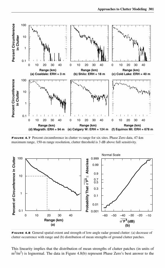
Approaches to Clutter Modeling 301

This linearity implies that the distribution of mean strengths of clutter patches (in units ofm2/m2) is lognormal. The data in Figure 4.8(b) represent Phase Zero’s best answer to the

Figure 4.7 Percent circumference in clutter vs range for six sites. Phase Zero data, 47-km maximum range, 150-m range resolution, clutter threshold is 3 dB above full sensitivity.

Figure 4.8 General spatial extent and strength of low-angle radar ground clutter: (a) decrease of clutter occurrence with range and (b) distribution of mean strengths of ground clutter patches.

0 10 20 30 40 0 10 20 30 40 0 10 20 30 40

0 10 20 30 40 0 10 20 30 40 0 10 20 30 40

Range (km)(d) Magrath: ERH = 94 m

Range (km)(e) Calgary W: ERH = 124 m

Range (km)(f) Equinox Mt: ERH = 678 m

Range (km)(a) Coaldale: ERH = 3 m

Range (km)(b) Shilo: ERH = 18 m

Range (km)(c) Cold Lake: ERH = 40 m

100

10

1

0.1

100

10

1

0.1

Per

cen

t C

ircu

mfe

ren

cein

Clu

tter

Per

cen

t C

ircu

mfe

ren

cein

Clu

tter

Normal Scale

0.001

0.01

0.1

0.3

0.7

0.9

0.99

0.999

F4 (dB)(b)

–60 –50 –40 –30 –20 –10Per

cen

t o

f C

ircu

mfe

ren

ce in

Clu

tter

0 10 20 30 40

0.1

1

10

100

Pro

bab

ility

Th

at

F4 A

bsc

issa

Range (km)(a)

0.5

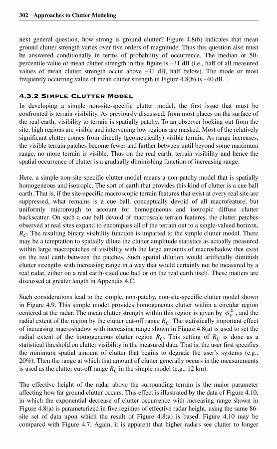
302 Approaches to Clutter Modeling

next general question, how strong is ground clutter? Figure 4.8(b) indicates that meanground clutter strength varies over five orders of magnitude. Thus this question also mustbe answered conditionally in terms of probability of occurrence. The median or 50-percentile value of mean clutter strength in this figure is –31 dB (i.e., half of all measuredvalues of mean clutter strength occur above –31 dB, half below). The mode or mostfrequently occurring value of mean clutter strength in Figure 4.8(b) is –40 dB.

4.3.2 Simple Clutter ModelIn developing a simple non-site-specific clutter model, the first issue that must beconfronted is terrain visibility. As previously discussed, from most places on the surface ofthe real earth, visibility to terrain is spatially patchy. To an observer looking out from thesite, high regions are visible and intervening low regions are masked. Most of the relativelysignificant clutter comes from directly (geometrically) visible terrain. As range increases,the visible terrain patches become fewer and farther between until beyond some maximumrange, no more terrain is visible. Thus on the real earth, terrain visibility and hence thespatial occurrence of clutter is a gradually diminishing function of increasing range.

Here, a simple non-site-specific clutter model means a non-patchy model that is spatiallyhomogeneous and isotropic. The sort of earth that provides this kind of clutter is a cue ballearth. That is, if the site-specific macroscopic terrain features that exist at every real site aresuppressed, what remains is a cue ball, conceptually devoid of all macrofeature, butuniformly microrough to account for homogeneous and isotropic diffuse clutterbackscatter. On such a cue ball devoid of macroscale terrain features, the clutter patchesobserved at real sites expand to encompass all of the terrain out to a single-valued horizon,RC. The resulting binary visibility function is imparted to the simple clutter model. Theremay be a temptation to spatially dilute the clutter amplitude statistics as actually measuredwithin large macropatches of visibility with the large amounts of macroshadow that existon the real earth between the patches. Such spatial dilution would artificially diminishclutter strengths with increasing range in a way that would certainly not be measured by areal radar, either on a real earth-sized cue ball or on the real earth itself. These matters arediscussed at greater length in Appendix 4.C.

Such considerations lead to the simple, non-patchy, non-site-specific clutter model shownin Figure 4.9. This simple model provides homogeneous clutter within a circular regioncentered at the radar. The mean clutter strength within this region is given by , and theradial extent of the region by the clutter cut-off range RC. The statistically important effectof increasing macroshadow with increasing range shown in Figure 4.8(a) is used to set theradial extent of the homogeneous clutter region RC. This setting of RC is done as astatistical threshold on clutter visibility in the measured data. That is, the user first specifiesthe minimum spatial amount of clutter that begins to degrade the user’s systems (e.g.,20%). Then the range at which that amount of clutter generally occurs in the measurementsis used as the clutter cut-off range RC in the simple model (e.g., 12 km).

The effective height of the radar above the surrounding terrain is the major parameteraffecting how far ground clutter occurs. This effect is illustrated by the data of Figure 4.10,in which the exponential decrease of clutter occurrence with increasing range shown inFigure 4.8(a) is parameterized in five regimes of effective radar height, using the same 86-site set of data upon which the result of Figure 4.8(a) is based. Figure 4.10 may becompared with Figure 4.7. Again, it is apparent that higher radars see clutter to longer

σ °w

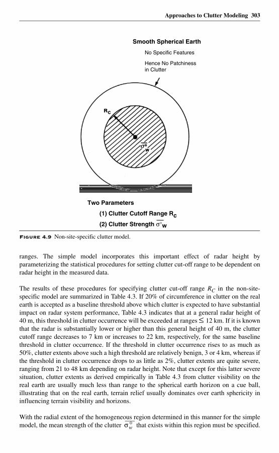
Approaches to Clutter Modeling 303

ranges. The simple model incorporates this important effect of radar height byparameterizing the statistical procedures for setting clutter cut-off range to be dependent onradar height in the measured data.

The results of these procedures for specifying clutter cut-off range RC in the non-site-specific model are summarized in Table 4.3. If 20% of circumference in clutter on the realearth is accepted as a baseline threshold above which clutter is expected to have substantialimpact on radar system performance, Table 4.3 indicates that at a general radar height of40 m, this threshold in clutter occurrence will be exceeded at ranges ≤ 12 km. If it is knownthat the radar is substantially lower or higher than this general height of 40 m, the cluttercutoff range decreases to 7 km or increases to 22 km, respectively, for the same baselinethreshold in clutter occurrence. If the threshold in clutter occurrence rises to as much as50%, clutter extents above such a high threshold are relatively benign, 3 or 4 km, whereas ifthe threshold in clutter occurrence drops to as little as 2%, clutter extents are quite severe,ranging from 21 to 48 km depending on radar height. Note that except for this latter severesituation, clutter extents as derived empirically in Table 4.3 from clutter visibility on thereal earth are usually much less than range to the spherical earth horizon on a cue ball,illustrating that on the real earth, terrain relief usually dominates over earth sphericity ininfluencing terrain visibility and horizons.

With the radial extent of the homogeneous region determined in this manner for the simplemodel, the mean strength of the clutter that exists within this region must be specified.

Figure 4.9 Non-site-specific clutter model.

Smooth Spherical Earth

No Specific Features

Hence No Patchinessin Clutter

Two Parameters

(1) Clutter Cutoff Range Rc(2) Clutter Strength σ°w

σ °w

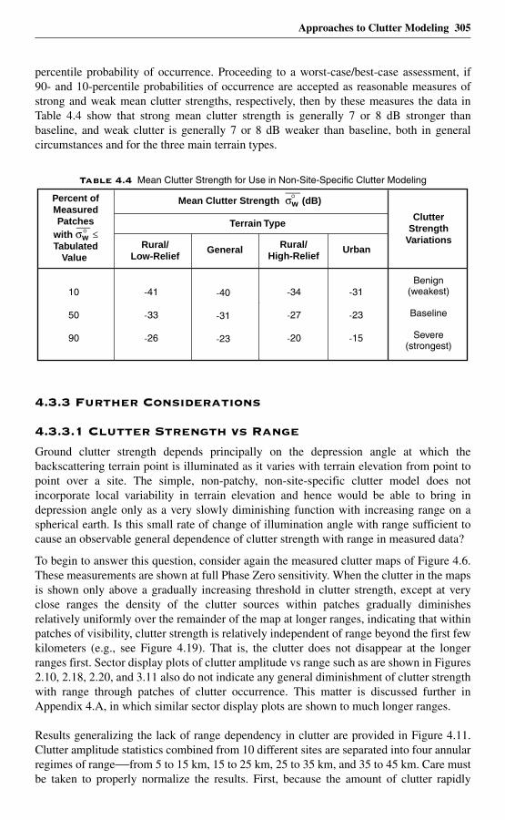
Approaches to Clutter Modeling 305

percentile probability of occurrence. Proceeding to a worst-case/best-case assessment, if90- and 10-percentile probabilities of occurrence are accepted as reasonable measures ofstrong and weak mean clutter strengths, respectively, then by these measures the data inTable 4.4 show that strong mean clutter strength is generally 7 or 8 dB stronger thanbaseline, and weak clutter is generally 7 or 8 dB weaker than baseline, both in generalcircumstances and for the three main terrain types.

4.3.3 Further Considerations

4.3.3.1 Clutter Strength vs Range

Ground clutter strength depends principally on the depression angle at which thebackscattering terrain point is illuminated as it varies with terrain elevation from point topoint over a site. The simple, non-patchy, non-site-specific clutter model does notincorporate local variability in terrain elevation and hence would be able to bring indepression angle only as a very slowly diminishing function with increasing range on aspherical earth. Is this small rate of change of illumination angle with range sufficient tocause an observable general dependence of clutter strength with range in measured data?

To begin to answer this question, consider again the measured clutter maps of Figure 4.6.These measurements are shown at full Phase Zero sensitivity. When the clutter in the mapsis shown only above a gradually increasing threshold in clutter strength, except at veryclose ranges the density of the clutter sources within patches gradually diminishesrelatively uniformly over the remainder of the map at longer ranges, indicating that withinpatches of visibility, clutter strength is relatively independent of range beyond the first fewkilometers (e.g., see Figure 4.19). That is, the clutter does not disappear at the longerranges first. Sector display plots of clutter amplitude vs range such as are shown in Figures2.10, 2.18, 2.20, and 3.11 also do not indicate any general diminishment of clutter strengthwith range through patches of clutter occurrence. This matter is discussed further inAppendix 4.A, in which similar sector display plots are shown to much longer ranges.

Results generalizing the lack of range dependency in clutter are provided in Figure 4.11.Clutter amplitude statistics combined from 10 different sites are separated into four annularregimes of range—from 5 to 15 km, 15 to 25 km, 25 to 35 km, and 35 to 45 km. Care mustbe taken to properly normalize the results. First, because the amount of clutter rapidly

Table 4.4 Mean Clutter Strength for Use in Non-Site-Specific Clutter Modeling

Mean Clutter Strength (dB)

Terrain Type

Percent ofMeasuredPatches

with σw ≤Tabulated

Value Rural/

Low-ReliefGeneral Rural/

High-Relief

ClutterStrength

Variations

10

50

90

-41

-33

-26

-40

-31

-23

-34

-27

-20

-31

-23

-15

Benign(weakest)

Baseline

Severe(strongest)

Urban

°

°σw

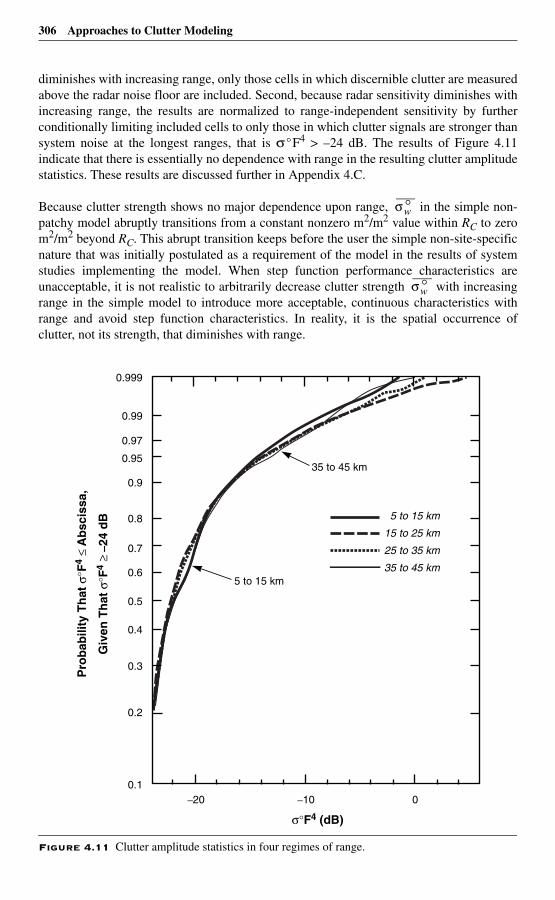
306 Approaches to Clutter Modeling

diminishes with increasing range, only those cells in which discernible clutter are measuredabove the radar noise floor are included. Second, because radar sensitivity diminishes withincreasing range, the results are normalized to range-independent sensitivity by furtherconditionally limiting included cells to only those in which clutter signals are stronger thansystem noise at the longest ranges, that is σ°F4 > –24 dB. The results of Figure 4.11indicate that there is essentially no dependence with range in the resulting clutter amplitudestatistics. These results are discussed further in Appendix 4.C.

Because clutter strength shows no major dependence upon range, in the simple non-patchy model abruptly transitions from a constant nonzero m2/m2 value within RC to zerom2/m2 beyond RC. This abrupt transition keeps before the user the simple non-site-specificnature that was initially postulated as a requirement of the model in the results of systemstudies implementing the model. When step function performance characteristics areunacceptable, it is not realistic to arbitrarily decrease clutter strength with increasingrange in the simple model to introduce more acceptable, continuous characteristics withrange and avoid step function characteristics. In reality, it is the spatial occurrence ofclutter, not its strength, that diminishes with range.

Figure 4.11 Clutter amplitude statistics in four regimes of range.

σ °w

σ °w

–20 –10 0

0.999

0.99

0.97

0.95

0.9

0.8

0.7

0.6

0.5

0.4

0.3

0.2

0.1

σ°F4 (dB)

Pro

bab

ility

Th

at σ

°F4

≤ A

bsc

issa

,

Giv

en T

hat

σ°F

4 ≥

–24

dB 5 to 15 km

15 to 25 km

25 to 35 km

35 to 45 km5 to 15 km

35 to 45 km

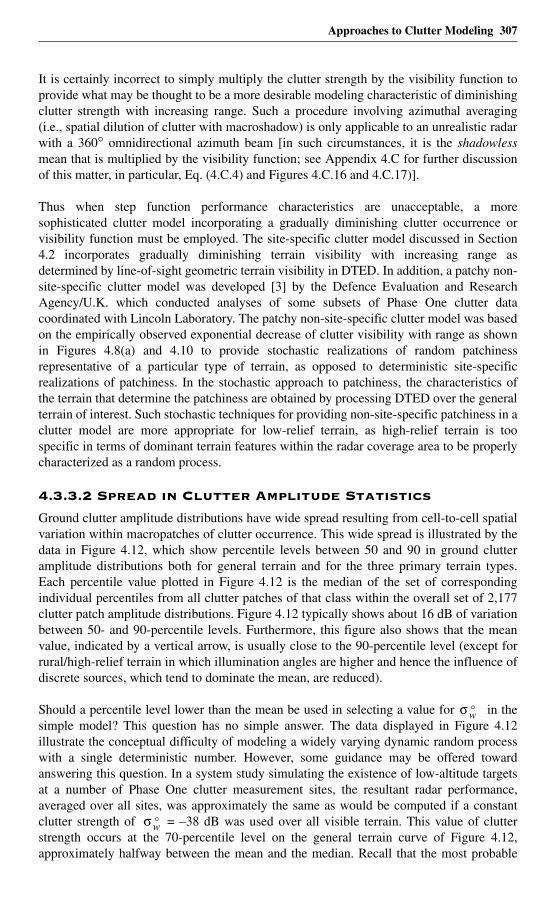
Approaches to Clutter Modeling 307

It is certainly incorrect to simply multiply the clutter strength by the visibility function toprovide what may be thought to be a more desirable modeling characteristic of diminishingclutter strength with increasing range. Such a procedure involving azimuthal averaging(i.e., spatial dilution of clutter with macroshadow) is only applicable to an unrealistic radarwith a 360° omnidirectional azimuth beam [in such circumstances, it is the shadowlessmean that is multiplied by the visibility function; see Appendix 4.C for further discussionof this matter, in particular, Eq. (4.C.4) and Figures 4.C.16 and 4.C.17)].

Thus when step function performance characteristics are unacceptable, a moresophisticated clutter model incorporating a gradually diminishing clutter occurrence orvisibility function must be employed. The site-specific clutter model discussed in Section4.2 incorporates gradually diminishing terrain visibility with increasing range asdetermined by line-of-sight geometric terrain visibility in DTED. In addition, a patchy non-site-specific clutter model was developed [3] by the Defence Evaluation and ResearchAgency/U.K. which conducted analyses of some subsets of Phase One clutter datacoordinated with Lincoln Laboratory. The patchy non-site-specific clutter model was basedon the empirically observed exponential decrease of clutter visibility with range as shownin Figures 4.8(a) and 4.10 to provide stochastic realizations of random patchinessrepresentative of a particular type of terrain, as opposed to deterministic site-specificrealizations of patchiness. In the stochastic approach to patchiness, the characteristics ofthe terrain that determine the patchiness are obtained by processing DTED over the generalterrain of interest. Such stochastic techniques for providing non-site-specific patchiness in aclutter model are more appropriate for low-relief terrain, as high-relief terrain is toospecific in terms of dominant terrain features within the radar coverage area to be properlycharacterized as a random process.

4.3.3.2 Spread in Clutter Amplitude Statistics

Ground clutter amplitude distributions have wide spread resulting from cell-to-cell spatialvariation within macropatches of clutter occurrence. This wide spread is illustrated by thedata in Figure 4.12, which show percentile levels between 50 and 90 in ground clutteramplitude distributions both for general terrain and for the three primary terrain types.Each percentile value plotted in Figure 4.12 is the median of the set of correspondingindividual percentiles from all clutter patches of that class within the overall set of 2,177clutter patch amplitude distributions. Figure 4.12 typically shows about 16 dB of variationbetween 50- and 90-percentile levels. Furthermore, this figure also shows that the meanvalue, indicated by a vertical arrow, is usually close to the 90-percentile level (except forrural/high-relief terrain in which illumination angles are higher and hence the influence ofdiscrete sources, which tend to dominate the mean, are reduced).

Should a percentile level lower than the mean be used in selecting a value for in thesimple model? This question has no simple answer. The data displayed in Figure 4.12illustrate the conceptual difficulty of modeling a widely varying dynamic random processwith a single deterministic number. However, some guidance may be offered towardanswering this question. In a system study simulating the existence of low-altitude targetsat a number of Phase One clutter measurement sites, the resultant radar performance,averaged over all sites, was approximately the same as would be computed if a constantclutter strength of = –38 dB was used over all visible terrain. This value of clutterstrength occurs at the 70-percentile level on the general terrain curve of Figure 4.12,approximately halfway between the mean and the median. Recall that the most probable

σ °w

σ °w

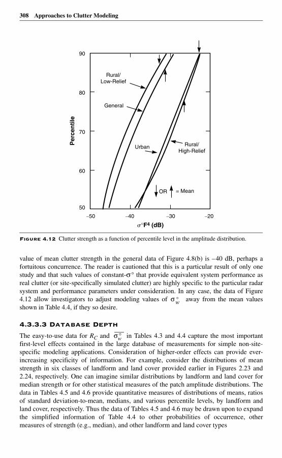
308 Approaches to Clutter Modeling

value of mean clutter strength in the general data of Figure 4.8(b) is –40 dB, perhaps afortuitous concurrence. The reader is cautioned that this is a particular result of only onestudy and that such values of constant-σ° that provide equivalent system performance asreal clutter (or site-specifically simulated clutter) are highly specific to the particular radarsystem and performance parameters under consideration. In any case, the data of Figure4.12 allow investigators to adjust modeling values of away from the mean valuesshown in Table 4.4, if they so desire.

4.3.3.3 Database Depth

The easy-to-use data for RC and in Tables 4.3 and 4.4 capture the most importantfirst-level effects contained in the large database of measurements for simple non-site-specific modeling applications. Consideration of higher-order effects can provide ever-increasing specificity of information. For example, consider the distributions of meanstrength in six classes of landform and land cover provided earlier in Figures 2.23 and2.24, respectively. One can imagine similar distributions by landform and land cover formedian strength or for other statistical measures of the patch amplitude distributions. Thedata in Tables 4.5 and 4.6 provide quantitative measures of distributions of means, ratiosof standard deviation-to-mean, medians, and various percentile levels, by landform andland cover, respectively. Thus the data of Tables 4.5 and 4.6 may be drawn upon to expandthe simplified information of Table 4.4 to other probabilities of occurrence, othermeasures of strength (e.g., median), and other landform and land cover types

Figure 4.12 Clutter strength as a function of percentile level in the amplitude distribution.

�°F4 (dB)

Per

cen

tile

–50 –40 –30 –20

50

60

70

80

90

Rural/Low-Relief

General

Urban Rural/High-Relief

= MeanOR

σ °w

σ °w

Approaches to Clutter Modeling 309

The statistical attributes shown in the second column of Tables 4.5 and 4.6 are now definedmore explicitly. Observe in Figures 2.23 and 2.24 that the distributions are approximatelylognormal. As a result, it is useful to define the mean and standard deviation of thenormally distributed logarithmic quantity. These two quantities are shown as the first (i.e.,top-most) and second attributes for each patch amplitude statistic. The third attribute shownis the median, which itself just transforms logarithmically. If the logarithmic quantity isnormally and hence symmetrically distributed, its mean and median must be identical. Thedata in Tables 4.5 and 4.6 indicate that these two quantities (i.e., the first and thirdattributes, respectively) are, indeed, often nearly equal. Once it is assumed that thedistribution is approximately lognormal, all other attributes of the distributions of both thelogarithmic quantity and the more fundamental underlying linear quantity immediatelyfollow from the first and second attributes provided in Tables 4.5 and 4.6. However, thefourth and final attribute for each patch amplitude statistic shown is the actual empiricalmean of the basic linear quantity, which can be used either directly in its own right or as afurther check on the degree of goodness of the approximating lognormal distributions.

Now consider some of the trends with landform contained in the data of Table 4.5, whereterrain slopes rise monotonically with landform class, left to right, from less than 1° forlevel terrain to between 10° and 35° for steep terrain (see Figure 2.23). Consider themedian of M samples within a particular landform class of a given statistic (e.g., mean) of aclutter amplitude distribution as an easy-to-understand attribute, in that half the samplesoccur above the median level and half below. The median attribute is shown in increasingorder of landform as the third row of numbers for each patch amplitude statistic in Table4.5. Thus, as terrain slopes rise from level to steep, the third rows of the table show that (1)mean strengths rise over the 10-dB range from –33 to –23 dB; (2) median strengths riseover the 15-dB range from –48 to –33 dB; (3) spreads in amplitude distributions asmeasured by ratio of standard deviation-to-mean fall from 7 to 3 dB, spreads as measuredby ratio of 99.9- to 50-percentile fall from 33 to 22 dB, and spreads as measured by ratio ofmean-to-median fall from 15 to 10 dB. All the trends are monotonic with increasing terrainsteepness as specified by the median value from a large number M of individual patchmeasurements within each landform class.

In considering increasing specificity of information, recall that all the non-site-specificinformation presented in this section has been derived from X-band measurements.However, when considering that mean strengths from the three general terrain types ofrural/low-relief, rural/high-relief, and urban are largely frequency independent, and that thesimple model is already averaging out much fine-scaled variation, it is not unrealistic toapply the simple model across the general microwave regime. Investigators who wish tointroduce more specific frequency dependence in non-site-specific investigation may, as abeginning, be guided by the multifrequency mean data of Table 4.2.

4.3.4 SummaryThe considerations guiding the development of the simple, non-angle-specific cluttermodeling information presented in Section 4.3 are now summarized. The objective is toinvest a simple clutter model with important general attributes as they have come to beunderstood in investigating the large database of clutter measurements. Of first-orderimportance is to distinguish between where the clutter occurs and its strength, given that itoccurs. The simple, non-patchy model of Section 4.3.2 maintains this distinction by firstspecifying clutter cut-off range based on the measurements of clutter visibility, and then

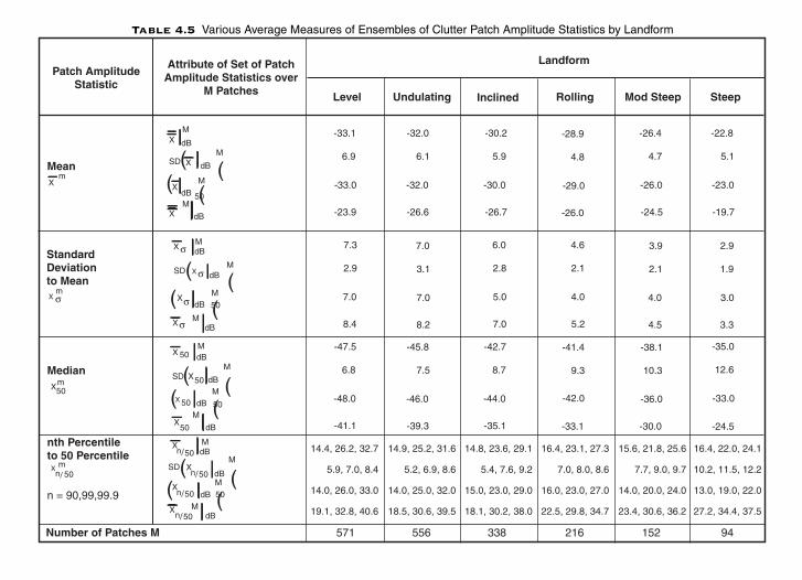
Table 4.5 Various Average Measures of Ensembles of Clutter Patch Amplitude Statistics by Landform

Meanm

X

Patch AmplitudeStatistic

Attribute of Set of PatchAmplitude Statistics over

M Patches

Landform

Level Undulating Rolling Mod Steep Steep

-33.1

6.9

-33.0

-23.9

-32.0

6.1

-32.0

-26.6

-30.2

5.9

-30.0

-26.7

-26.4

4.7

-26.0

-24.5

-22.8

5.1

-23.0

-19.7

StandardDeviationto Mean

mX σ

Inclined

-28.9

4.8

-29.0

-26.0

7.3

2.9

7.0

8.4

7.0

3.1

7.0

8.2

6.0

2.8

5.0

7.0

4.6

2.1

4.0

5.2

3.9

2.1

4.0

4.5

2.9

1.9

3.0

3.3

MedianmX50

-47.5

6.8

-48.0

-41.1

-45.8

7.5

-46.0

-39.3

-42.7

8.7

-44.0

-35.1

-41.4

9.3

-42.0

-33.1

-38.1

10.3

-36.0

-30.0

-35.0

12.6

-33.0

-24.5

Number of Patches M 571 556 338 216 152 94

X σMdB

SD X σ dBM

Xσ dBM

50

X Mσ dB

( (

( (

X 50MdB

SD X50 dB

M

X 50 dBM

50

XM

50 dB

((

((

nth Percentileto 50 Percentile

n = 90,99,99.9

mXn 50/

MdB

SDdB

M

dB

M50

MdB

Xn 50/

Xn 50/

Xn 50/

Xn 50/

( (

( (

XM

dB

SD X dB

M

XdB

M

50

X dB

((

((

M

14.4, 26.2, 32.7

5.9, 7.0, 8.4

14.0, 26.0, 33.0

19.1, 32.8, 40.6

14.9, 25.2, 31.6

5.2, 6.9, 8.6

14.0, 25.0, 32.0

18.5, 30.6, 39.5

14.8, 23.6, 29.1

5.4, 7.6, 9.2

15.0, 23.0, 29.0

18.1, 30.2, 38.0

16.4, 23.1, 27.3

7.0, 8.0, 8.6

16.0, 23.0, 27.0

22.5, 29.8, 34.7

15.6, 21.8, 25.6

7.7, 9.0, 9.7

14.0, 20.0, 24.0

23.4, 30.6, 36.2

16.4, 22.0, 24.1

10.2, 11.5, 12.2

13.0, 19.0, 22.0

27.2, 34.4, 37.5

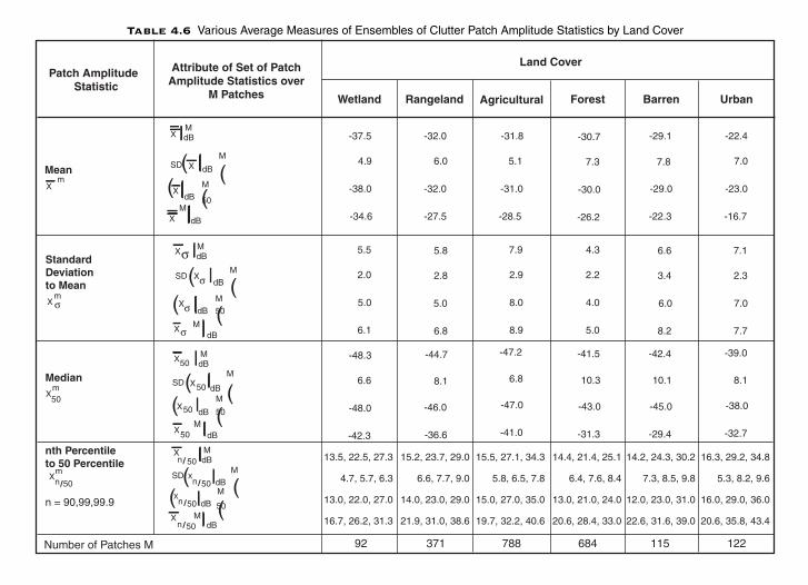
Table 4.6 Various Average Measures of Ensembles of Clutter Patch Amplitude Statistics by Land Cover

Meanm

X

Patch Amplitude Statistic

Attribute of Set of PatchAmplitude Statistics over

M Patches

Land Cover

Wetland Rangeland Forest Barren Urban

-37.5

4.9

-38.0

-34.6

-32.0

6.0

-32.0

-27.5

-31.8

5.1

-31.0

-28.5

-29.1

7.8

-29.0

-22.3

-22.4

7.0

-23.0

-16.7

StandardDeviationto Mean

mX σ

Agricultural

-30.7

7.3

-30.0

-26.2

5.5

2.0

5.0

6.1

5.8

2.8

5.0

6.8

7.9

2.9

8.0

8.9

4.3

2.2

4.0

5.0

6.6

3.4

6.0

8.2

7.1

2.3

7.0

7.7

Medianm

X50

-48.3

6.6

-48.0

-42.3

-44.7

8.1

-46.0

-36.6

-47.2

6.8

-47.0

-41.0

-41.5

10.3

-43.0

-31.3

-42.4

10.1

-45.0

-29.4

-39.0

8.1

-38.0

-32.7

Number of Patches M

13.5, 22.5, 27.3

4.7, 5.7, 6.3

13.0, 22.0, 27.0

16.7, 26.2, 31.3

15.2, 23.7, 29.0

6.6, 7.7, 9.0

14.0, 23.0, 29.0

21.9, 31.0, 38.6

15.5, 27.1, 34.3

5.8, 6.5, 7.8

15.0, 27.0, 35.0

19.7, 32.2, 40.6

14.4, 21.4, 25.1

6.4, 7.6, 8.4

13.0, 21.0, 24.0

20.6, 28.4, 33.0

14.2, 24.3, 30.2

7.3, 8.5, 9.8

12.0, 23.0, 31.0

22.6, 31.6, 39.0

16.3, 29.2, 34.8

5.3, 8.2, 9.6

16.0, 29.0, 36.0

20.6, 35.8, 43.4

92 371 788 684 115 122

XMdB

SD X dB

M

XdB

M

50

X dB

((

((

M

XσMdB

SD Xσ dB

M

Xσ dBM

50

X Mσ dB

( (

( (

X50MdB

SD X50 dB

M

X50 dB

M

50

XM

50 dB

( (

( (

MdB

SDdB

M

dB

M

50M

dBX

n 50/

Xn 50/

Xn 50/

Xn 50/

( ((

nth Percentileto 50 Percentile

n = 90,99,99.9

mX

n 50/

(

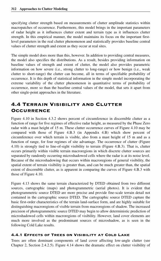
312 Approaches to Clutter Modeling

specifying clutter strength based on measurements of clutter amplitude statistics withinmacropatches of occurrence. Furthermore, this model brings in the important parametersof radar height as it influences clutter extent and terrain type as it influences clutterstrength. In this empirical manner, the model maintains its focus on the important first-level parameters in the real clutter phenomenon and statistically provides baseline centralvalues of clutter strength and extent as they occur at real sites.

The simple model does more than this, however. In addition to providing central measures,the model also specifies the distributions. As a result, besides providing information onbaseline values of strength and extent of clutter, the model also provides parametricinformation on how severe (i.e., strong clutter to long-range) or how benign (i.e., weakclutter to short-range) the clutter can become, all in terms of specifiable probability ofoccurrence. It is this depth of statistical information in the simple model incorporating theextreme variability of the clutter phenomenon in quantitative terms of probability ofoccurrence, more so than the baseline central values of the model, that sets it apart fromother single-point approaches in the literature.

4.4 Terrain Visibility and Clutter OccurrenceFigure 4.10 in Section 4.3.2 shows percent of circumference in discernible clutter as afunction of range for five regimes of effective radar height, as measured by the Phase Zeroradar with a mast height of 15 m. These clutter occurrence curves of Figure 4.10 may becompared with those of Figure 4.B.3 (in Appendix 4.B) which show percent ofcircumference over which terrain is visible, also from a mast height of 15 m and as afunction of range, for four regimes of site advantage. The occurrence of clutter (Figure4.10) is strongly tied to line-of-sight visibility to terrain (Figure 4.B.3). That is, clutteroccurs primarily within visible terrain macroregions in which discrete clutter sources areseparated by randomly occurring microshadowed cells where the radar is at its noise level.Because of the microshadowing that occurs within macroregions of general visibility, thespatial extent of terrain visibility is greater than, and can be much greater than, the spatialextent of discernible clutter, as is apparent in comparing the curves of Figure 4.B.3 withthose of Figure 4.10.

Figure 4.13 shows the same terrain characterized by DTED obtained from two differentsources, cartographic (maps) and photogrammetric (aerial photos). It is evident thatphotogrammetric source DTED are more precise and provide fine-scale terrain detail notcontained in the cartographic source DTED. The cartographic source DTED capture thebasic first-order characteristics of the terrain land-surface form, and are highly suitable fordistinguishing macroregions of visible terrain from macroregions of shadow. The increasedprecision of photogrammetric source DTED may begin to allow deterministic prediction ofmicroshadowed cells within macroregions of visibility. However, land cover elements aremuch more involved as the predominant sources of microshadow, as is seen in thefollowing Cold Lake results.

4.4.1 Effects of Trees on Visibility at Cold LakeTrees are often dominant components of land cover affecting low-angle clutter (seeChapter 2, Section 2.4.2.5). Figure 4.14 shows the dramatic effect on clutter visibility of

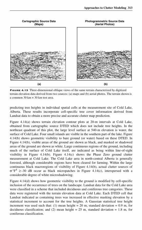
Approaches to Clutter Modeling 313

predicting tree heights in individual spatial cells at the measurement site of Cold Lake,Alberta. These results incorporate cell-specific tree cover information derived fromLandsat data to obtain a more precise and accurate clutter map prediction.

Figure 4.14(a) shows terrain elevation contour plots at 20-m intervals at Cold Lake,obtained from cartographic source DTED which does not include tree heights. In thenortheast quadrant of this plot, the large level surface at 540-m elevation is water, thesurface of Cold Lake. Four small islands are visible in the southern part of the lake. Figure4.14(b) shows geometric visibility to bare ground (or water) based on these DTED. InFigure 4.14(b), visible areas of the ground are shown as black, and masked or shadowedareas of the ground are shown as white. Large continuous regions of the ground, includingmuch of the surface of Cold Lake itself, are indicated as being within line-of-sightvisibility in Figure 4.14(b). Figure 4.14(c) shows the Phase Zero ground cluttermeasurement at Cold Lake. The Cold Lake area in north-central Alberta is generallyforested, although considerable regions have been cleared for farming. Within the largecontinuous black macroregions of visibility of Figure 4.14(b), actual clutter sources ofσ °F4 ≥–30 dB occur as black micropatches in Figure 4.14(c), interspersed with aconsiderable degree of white microshadowing.

Figure 4.14(d) shows how geometric visibility to the ground is modified by cell-specificinclusion of the occurrence of trees on the landscape. Landsat data for the Cold Lake areawere classified in a scheme that included deciduous and coniferous tree categories. Thesedata were registered with the terrain elevation data at Cold Lake. Each DTED cell thatLandsat indicated as containing trees was increased in effective masking elevation by astatistical increment to account for the tree heights. A Gaussian statistical tree heightincrement was used such that: (1) mean height = 20 m, standard deviation = 0.9 m, fordeciduous classification; and (2) mean height = 25 m, standard deviation = 1.8 m, forconiferous classification.

Figure 4.13 Three-dimensional oblique views of the same terrain characterized by digitized terrain elevation data derived from two sources: (a) maps and (b) aerial photos. The terrain shown is a common 30 km × 30 km test area.

(a) (b)

Cartographic Source Data(Maps)

Photogrammetric Source Data(Aerial Photos)

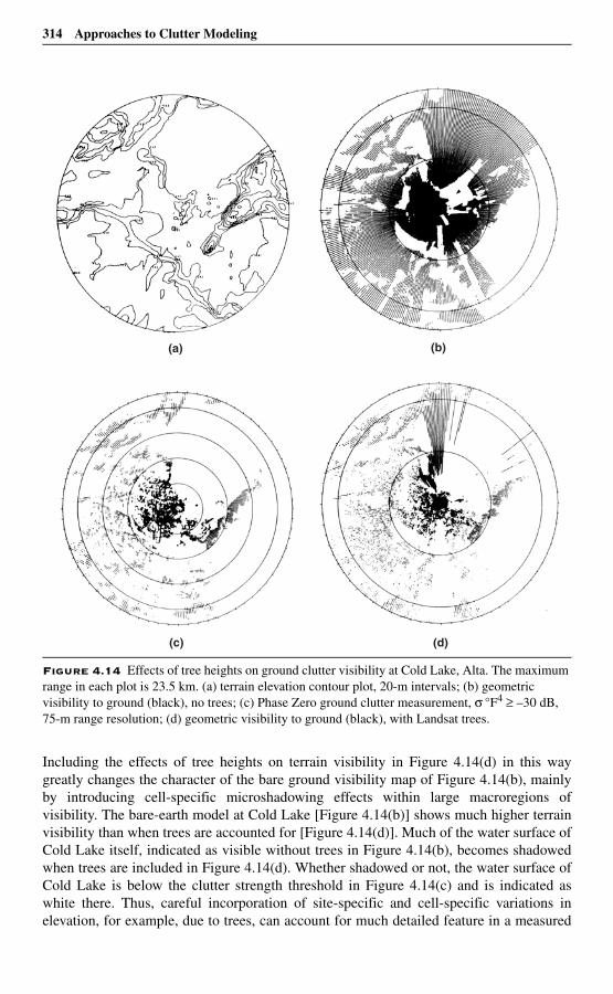
314 Approaches to Clutter Modeling

Including the effects of tree heights on terrain visibility in Figure 4.14(d) in this waygreatly changes the character of the bare ground visibility map of Figure 4.14(b), mainlyby introducing cell-specific microshadowing effects within large macroregions ofvisibility. The bare-earth model at Cold Lake [Figure 4.14(b)] shows much higher terrainvisibility than when trees are accounted for [Figure 4.14(d)]. Much of the water surface ofCold Lake itself, indicated as visible without trees in Figure 4.14(b), becomes shadowedwhen trees are included in Figure 4.14(d). Whether shadowed or not, the water surface ofCold Lake is below the clutter strength threshold in Figure 4.14(c) and is indicated aswhite there. Thus, careful incorporation of site-specific and cell-specific variations inelevation, for example, due to trees, can account for much detailed feature in a measured

Figure 4.14 Effects of tree heights on ground clutter visibility at Cold Lake, Alta. The maximum range in each plot is 23.5 km. (a) terrain elevation contour plot, 20-m intervals; (b) geometric visibility to ground (black), no trees; (c) Phase Zero ground clutter measurement, σ °F4 ≥ –30 dB, 75-m range resolution; (d) geometric visibility to ground (black), with Landsat trees.

(b)

(c) (d)

(a)

Approaches to Clutter Modeling 315

ground clutter map, based on geometric visibility considerations alone without anyrecourse to propagation or scattering physics.

4.4.2 Decreasing Shadowing with Increasing Site HeightAlthough there exists much correlation in terms of general features between the measuredCold Lake clutter map of Figure 4.14(c) and the predicted map inclusive of tree heighteffects of Figure 4.14(d), careful examination indicates that on a more detailed cell-by-cellbasis the correlation in these maps deteriorates. Successful reduction of cluttermeasurement data in a cell-specific manner in which measured clutter strength in a cell isassociated with cell-specific geometric effects such as tree height and grazing angle wouldrequire terrain descriptive Geographic Information System (GIS) data of very highprecision and accuracy.

The reduction of measured clutter data as described in this book uses available DTEDmore simply to predict boundaries of macroregions of general terrain visibility, which aredenoted as clutter patches. Then all of the measured clutter data within the boundaries ofthe specified patch, including cells at radar noise level, are assembled in a histogram ofclutter strengths associated with the patch. Figure 4.15 shows six such measuredhistograms, one for each of six different sites (including Cold Lake) in order of increasingeffective radar height. In these histograms, the 50-, 90-, and 99-percentile levels are shownas vertical dotted lines; the mean strength is shown as a vertical dashed line; and bins tothe left side of the histogram that are significantly contaminated by radar noise samplesare doubly underlined. Figure 4.16 shows the cumulative distributions above the highestnoise contaminated bin for each of these six patches. Table 4.7 shows the incidence ofmicroshadowing within each patch and its effect on the mean clutter strength of the patch.For example, the incidence of microshadowing for the Cold Lake patch for which theclutter strength histogram is shown in Figure 4.15(c) is 35%.

It is evident in these results that the incidence of microshadowing within clutter patchesdecreases rapidly with increasing effective radar height. At low sites such as Coaldale andShilo, the incidence of microshadowing can be very high (74% at Coaldale), but even so themean clutter strength of the patch as determined within the upper- and lower-bound limitsremains accurate (to within 0.014 dB at Coaldale). The mean strength of the patchdetermined in this manner includes the effects of microshadowing and is accurateindependent of the sensitivity of the measurement radar; so also is the cumulativedistribution for the patch (above the highest noise contaminated bin) as is shown in Figure4.16 and from which the Weibull shape parameter aw is obtained. The shadowless meanclutter data shown in Table 4.7 which do not include samples within the histogram at radarnoise level are highly dependent on the particular sensitivity of the measurement radarutilized and are not generally useful in clutter modeling (although such data are ofteninappropriately used in the existing clutter literature).

4.4.3 Vertical Objects on Level Terrain at AltonaPrediction of clutter strengths based on the information provided in this book proceeds onthe basis of many measured patch histograms and cumulative distributions of clutterstrength such as are shown in Figures 4.15 and 4.16. Given the occurrence of a visibleterrain macroregion, the subsequent distribution of modeled clutter over the region isspecified as a broad Weibull distribution of appropriate shape parameter aw that includesthe distribution of microshadowed cells at the correct incidence of occurrence as Weibull

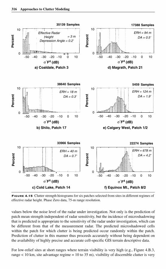
316 Approaches to Clutter Modeling

values below the noise level of the radar under investigation. Not only is the prediction ofpatch mean strength independent of radar sensitivity, but the incidence of microshadowingthat is predicted is appropriate to the sensitivity of the radar under investigation, which canbe different from that of the measurement radar. The predicted microshadowed cellswithin the patch for which clutter is being predicted occur randomly within the patch.Prediction of clutter in this manner thus proceeds accurately without being dependent onthe availability of highly precise and accurate cell-specific GIS terrain descriptive data.

For low-relief sites at short ranges where terrain visibility is very high (e.g., Figure 4.B.3,range < 10 km, site advantage regime = 10 to 35 m), visibility of discernible clutter is very

Figure 4.15 Clutter strength histograms for six patches selected from sites in different regimes of effective radar height. Phase Zero data, 75-m range resolution.

–50 –40 –30 –20 –10 0 10

Samples

Samples

Samples

σ˚F4 (dB)

–50 –40 –30 –20 –10 0 10

σ˚F4 (dB)

–50 –40 –30 –20 –10 0 10

σ˚F4 (dB)

–50 –40 –30 –20 –10 0 10

σ˚F4 (dB)

–50 –40 –30 –20 –10 0 10

σ˚F4 (dB)

–50 –40 –30 –20 –10 0 10

σ˚F4 (dB)

Per

cen

t

a) Coaldale, Patch 3

b) Shilo, Patch 17

c) Cold Lake, Patch 14

d) Magrath, Patch 21

e) Calgary West, Patch 1/2

f) Equinox Mt., Patch 8/2

10

0

Per

cen

t

10

0

Per

cen

t

10

0

Per

cen

t

10

0

Per

cen

t10

0

Per

cen

t

10

0

ERH = 18 m

DA = 0.3˚

Effective RadarHeight

Depression Angle = 0.2˚

ERH = 124 m

DA = 1.9˚

ERH = 94 m

DA = 0.5˚

ERH = 40 m

DA = 0.7˚

ERH = 678 m

DA = 4.2˚

= 3 m

35139

38640

33966

Samples

Samples

Samples

17388

5459

22274

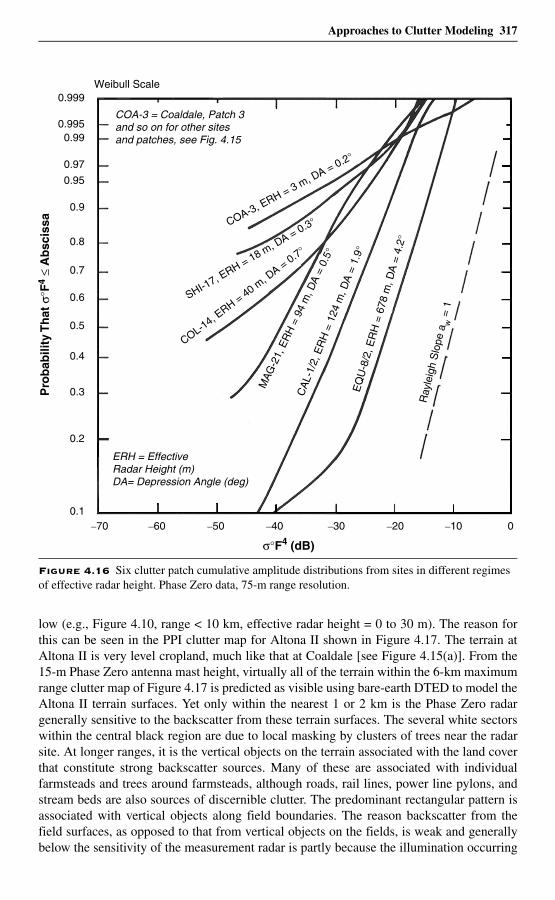
Approaches to Clutter Modeling 317

low (e.g., Figure 4.10, range < 10 km, effective radar height = 0 to 30 m). The reason forthis can be seen in the PPI clutter map for Altona II shown in Figure 4.17. The terrain atAltona II is very level cropland, much like that at Coaldale [see Figure 4.15(a)]. From the15-m Phase Zero antenna mast height, virtually all of the terrain within the 6-km maximumrange clutter map of Figure 4.17 is predicted as visible using bare-earth DTED to model theAltona II terrain surfaces. Yet only within the nearest 1 or 2 km is the Phase Zero radargenerally sensitive to the backscatter from these terrain surfaces. The several white sectorswithin the central black region are due to local masking by clusters of trees near the radarsite. At longer ranges, it is the vertical objects on the terrain associated with the land coverthat constitute strong backscatter sources. Many of these are associated with individualfarmsteads and trees around farmsteads, although roads, rail lines, power line pylons, andstream beds are also sources of discernible clutter. The predominant rectangular pattern isassociated with vertical objects along field boundaries. The reason backscatter from thefield surfaces, as opposed to that from vertical objects on the fields, is weak and generallybelow the sensitivity of the measurement radar is partly because the illumination occurring

Figure 4.16 Six clutter patch cumulative amplitude distributions from sites in different regimes of effective radar height. Phase Zero data, 75-m range resolution.

Pro

bab

ility

Th

at σ

°F4

≤ A

bsc

issa

σ°F4 (dB)

Weibull Scale

COA-3 = Coaldale, Patch 3and so on for other sitesand patches, see Fig. 4.15

ERH = EffectiveRadar Height (m)DA= Depression Angle (deg)

0.995

0.999

0.99

0.97

0.95

0.8

0.9

0.7

0.6

0.5

0.4

0.3

0.2

0.1–70 –60 –50 –40 –30 –20 0–10

COA-3, ERH = 3 m, D

A = 0.2°

SHI-17, E

RH = 18 m, DA = 0.3°

COL-14, ERH = 40 m

, DA = 0.7°

MAG

-21,

ER

H =

94

m, D

A =

0.5

°

CA

L-1/

2, E

RH

= 1

24 m

, DA

= 1

.9°

EQ

U-8

/2, E

RH

= 6

78 m

, DA

= 4

.2°

Ray

leig

h S

lope

aw

= 1

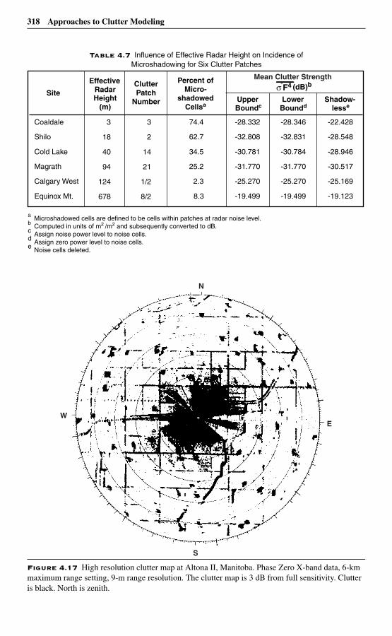
318 Approaches to Clutter Modeling

Table 4.7 Influence of Effective Radar Height on Incidence of Microshadowing for Six Clutter Patches

Figure 4.17 High resolution clutter map at Altona II, Manitoba. Phase Zero X-band data, 6-km maximum range setting, 9-m range resolution. The clutter map is 3 dB from full sensitivity. Clutter is black. North is zenith.

a Microshadowed cells are defined to be cells within patches at radar noise level.b Computed in units of m2 /m2 and subsequently converted to dB.c Assign noise power level to noise cells.d Assign zero power level to noise cells.e Noise cells deleted.

(dB)bF4Site

EffectiveRadarHeight

(m)

ClutterPatch

Number

Percent ofMicro-

shadowedCellsa

UpperBoundc Boundd

Lower Shadow-lesse

Coaldale

Shilo

Cold Lake

Magrath

Calgary West

Equinox Mt.

3

18

40

94

124

678

3

2

14

21

1/2

8/2

74.4

62.7

34.5

25.2

2.3

8.3

-28.332

-32.808

-30.781

-31.770

-25.270

-19.499

-28.346

-32.831

-30.784

-31.770

-25.270

-19.499

-22.428

-28.548

-28.946

-30.517

-25.169

-19.123

Mean Clutter Strength

σ̊

N

S

WE

Approaches to Clutter Modeling 319

beyond 1 or 2 km is very close to grazing incidence and partly because many of these lowsurfaces are shadowed by land cover features not included in DTED (e.g., road and railbeds) that are a few feet higher than the field surfaces proper.

Thus, all of the terrain in Figure 4.17 is within geometric line-of-sight visibility as modeledwith DTED, yet the clutter sources are predominantly vertical objects associated with landcover as they exist distributed over this nominally visible terrain. As a result, the extent ofdiscernible clutter (black) in Figure 4.17 is much less than the extent of nominally visibleterrain, and a very high incidence of white microshadowed cells occurs between the blackclutter cells.

4.4.4 SummaryDetermination of geometric terrain visibility in a bare-earth faceted terrain model based onDTED predicts general terrain regions in which clutter sources occur. Predicting theexistence of clutter thus arises from a set of conditional probabilities, in which the first andmost important condition for the existence of clutter at some spatial position is for thatposition to be geometrically visible. Consider again (see Section 4.3.1) that the probabilityof discernible clutter Pc is given by the probability that the terrain is geometrically visiblePv times the probability PD that the clutter strength is discernible, given that the terrain isvisible. As discussed in Section 4.3.1, PD is easily numerically evaluated, once theWeibull coefficients of the clutter and the noise level of the radar are specified.

Further conditions on clutter discernibility, in addition to the radar sensitivity at the pointunder consideration, are those associated with land cover, as discussed for Altona II andCold Lake, or conditions associated with propagation. For example, as discussed inChapter 3, at low radar frequencies such as VHF, little clutter may be received from low-relief terrain because terrain reflections prevent illumination of the terrain, even though itis within line-of-sight. Or some VHF clutter may be received from regions somewhatbeyond geometric visibility due to diffraction, if the radar sensitivity is high enough todiscern relatively weak clutter (clutter strength for shadowed terrain depends on depth ofshadow; see Appendix 4.D). The Phase One clutter data indicate that determination ofbare-earth terrain visibility is the most useful first step in understanding the spatialoccurrence of ground clutter, even at VHF. Effective radar height is the single most usefulparameter combining site height and mast height for specifying the extent in range towhich clutter occurs.

Increasingly precise and accurate terrain descriptive GIS data together with ever moreavailable computational power will allow increasingly accurate future specification of thelandform and land cover contents of individual clutter cells. Even with such increasedinformation, the extreme complexity of terrain will likely always require that the predictionof clutter strength from a cell (as opposed to the visibility of the cell) be based on astatistical approach. Whatever the level of fidelity of the available terrain descriptiveinformation, it is evident from the Cold Lake and Altona II results that geometricalconsiderations dominate the low-angle ground clutter phenomenon, and a realistic approachto clutter prediction needs to involve prediction of geometric terrain visibility as a first step,followed by a statistical determination of clutter strength based on terrain relief and theavailable land cover information. Although geometry is of first-order importance in thisprocess, once the realistic geometry is specified for a given radar observing the contents of agiven visible cell over a given profile, then as a higher-order matter considerations of

320 Approaches to Clutter Modeling

propagation, scattering, and absorption physics can be brought to bear to provide increasedunderstanding of the clutter strength phenomenon for that cell. But it is apparent thatattempts to model low-angle clutter based on propagation and scattering physics applied as afirst step to simplified or canonical representations of the earth that do not take into accountspecificities of geometry are foreordained to be exercises of the imagination.

4.5 Discrete vs Distributed Clutter

4.5.1 IntroductionIt has long been recognized that “. . . dominant land clutter signals are from discreteisolated targets . . . ”[4]. This section addresses important considerations involving themodeling of discrete clutter, as opposed to that of distributed clutter. A discrete clutter cellis an occasional, unusually strong, spatially isolated clutter cell for which the strong returnis typically associated with some large physical point object in the cell. Discrete clutter isalso occasionally referred to as point clutter or specular clutter in the literature. In contrast,distributed clutter is considered to be extensive in area over the clutter-producing surfacerather than being associated with particular points on the surface.

Before taking up the subject of approaches to modeling discrete clutter, it is necessary tofirst distinguish between conceptual models and empirical models. A conceptual cluttermodel is defined here as a hypothetical construct of the imagination that attempts to matchselected important observed features in measured clutter data. On the other hand, anempirical clutter model is tied more tightly to direct trend analyses in actual measuredclutter data, where the parametric trends observed in the data and their logicalinterrelationships and consequences themselves constitute the predictive clutter model. Anempirical model is based on reduction and analysis of measured clutter data, whereas aconceptual model can be postulated apart from measured data. In the empirical approach,any preconceived parametric relationships arising from postulated conceptualizedmodeling constructs that cannot be verified to exist in the measured clutter data are notallowed to have a place in the final empirical modeling apparatus. This book takes anempirical approach to generating clutter modeling information, including the modeling ofdiscrete clutter.

Discrete clutter was early addressed as being of serious systems consequence in land clutterin airborne radar. As discussed in Chapter 2 (see Sections 2.3.4.2 and 2.4.4.3), distributedland clutter occurring at higher depression angles characteristic of airborne radar is arelatively well-behaved quasi-homogeneous, quasi-Rayleigh process of relatively constantreturn, i.e., exhibiting only small cell-to-cell variability, for example as illustrated in the vs range data shown in Figure 2.20 as measured at Cazenovia. In such a well-behaved,relatively constant clutter background, occasional spatially isolated discrete cells of verymuch stronger clutter amplitude clearly stand out as being entirely different in kind fromthe surrounding weaker quasi-homogeneous clutter and are easily capturable in measureddata via spatial filtering and amplitude thresholding.

Various measurement programs were established to characterize discrete clutter in airborneradar [5, 6]. An elaborate, largely conceptual clutter model was developed at IIT ResearchInstitute (IITRI) for ground clutter in airborne radar including distributed and discretecomponents [7, 8]. The distributed component was modeled in terms of the backscattering

σ °

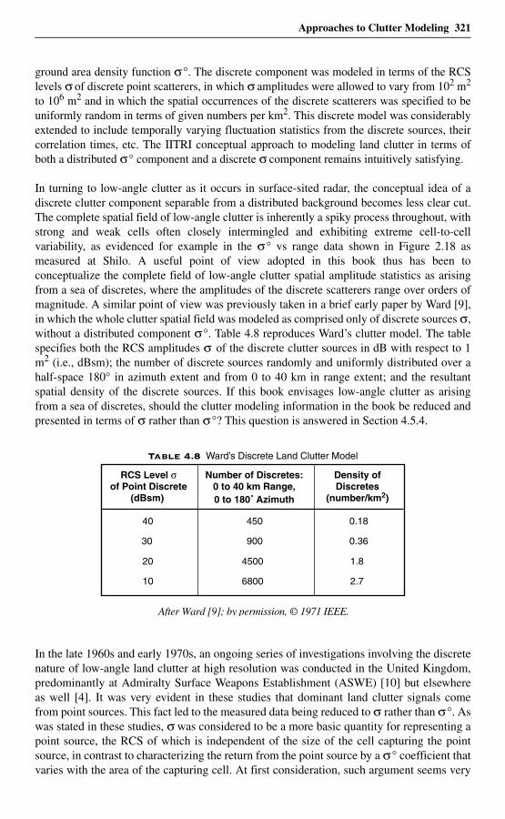
Approaches to Clutter Modeling 321

ground area density function σ°. The discrete component was modeled in terms of the RCSlevels σ of discrete point scatterers, in which σ amplitudes were allowed to vary from 102 m2

to 106 m2 and in which the spatial occurrences of the discrete scatterers was specified to beuniformly random in terms of given numbers per km2. This discrete model was considerablyextended to include temporally varying fluctuation statistics from the discrete sources, theircorrelation times, etc. The IITRI conceptual approach to modeling land clutter in terms ofboth a distributed σ° component and a discrete σ component remains intuitively satisfying.

In turning to low-angle clutter as it occurs in surface-sited radar, the conceptual idea of adiscrete clutter component separable from a distributed background becomes less clear cut.The complete spatial field of low-angle clutter is inherently a spiky process throughout, withstrong and weak cells often closely intermingled and exhibiting extreme cell-to-cellvariability, as evidenced for example in the σ° vs range data shown in Figure 2.18 asmeasured at Shilo. A useful point of view adopted in this book thus has been toconceptualize the complete field of low-angle clutter spatial amplitude statistics as arisingfrom a sea of discretes, where the amplitudes of the discrete scatterers range over orders ofmagnitude. A similar point of view was previously taken in a brief early paper by Ward [9],in which the whole clutter spatial field was modeled as comprised only of discrete sources σ,without a distributed component σ°. Table 4.8 reproduces Ward’s clutter model. The tablespecifies both the RCS amplitudes σ of the discrete clutter sources in dB with respect to 1m2 (i.e., dBsm); the number of discrete sources randomly and uniformly distributed over ahalf-space 180° in azimuth extent and from 0 to 40 km in range extent; and the resultantspatial density of the discrete sources. If this book envisages low-angle clutter as arisingfrom a sea of discretes, should the clutter modeling information in the book be reduced andpresented in terms of σ rather than σ°? This question is answered in Section 4.5.4.

In the late 1960s and early 1970s, an ongoing series of investigations involving the discretenature of low-angle land clutter at high resolution was conducted in the United Kingdom,predominantly at Admiralty Surface Weapons Establishment (ASWE) [10] but elsewhereas well [4]. It was very evident in these studies that dominant land clutter signals comefrom point sources. This fact led to the measured data being reduced to σ rather than σ°. Aswas stated in these studies, σ was considered to be a more basic quantity for representing apoint source, the RCS of which is independent of the size of the cell capturing the pointsource, in contrast to characterizing the return from the point source by a σ° coefficient thatvaries with the area of the capturing cell. At first consideration, such argument seems very

Table 4.8 Ward’s Discrete Land Clutter Model

RCS Level σof Point Discrete

(dBsm)

Number of Discretes:0 to 40 km Range,0 to 180˚ Azimuth

Density ofDiscretes

(number/km2)

40

30

20

10

450

900

4500

6800

0.18

0.36

1.8

2.7

322 Approaches to Clutter Modeling

reasonable. Again, should the modeling information in this book be presented in terms of σrather than σ°? Although deferring the answer to Section 4.5.4, we begin to address suchmatters in what follows.

Although it is possible to postulate a conceptual clutter model comprising both a distributedσ°component and a discrete σ component, it is far from straightforward to separatedistributed from discrete clutter in measured low-angle clutter data. The difficulty inmeaningfully or usefully effecting such a separation is not widely recognized, althoughSchleher does so as indicated in the following direct quotation: “Note that mostexperimental [land] clutter measurements . . . include composite discrete and distributedclutter, which cannot be separated into component parts, and hence measurement statisticsof parameters such as σ° . . . represent combined statistical data” [11]. For example, theAWSE measurements of discrete clutter mentioned previously were entirely reduced interms of σ, without any attempt to reduce a separate σ° component that might be moreappropriate at weaker levels.

The inherent spikiness of low-angle clutter is the basic reason why it is difficult tomeaningfully separate discrete and distributed components in low-angle clutter simply on thebasis of recognizable qualitative differences as exist in higher-angle clutter. Certainly, withoutrecourse to detailed ground truth information, nothing can be said about how point-like anyclutter source is beyond the spatial resolution of the measurement. It may be thought from atheoretical point of view that measurements of the same clutter at increasing resolution couldfind point sources by looking for cells, each providing a constant level of clutter RCS σindependent of the capturing cell size. In practice, Phase One measurements of the same clutterregion at both 150-m and 15-m range resolution both reveal cell-to-cell variations in spikiness,with the rate of variation 10 times faster at 15-m resolution than at 150-m resolution, in whichit is seldom evident that a particular 15-m cell within any 10-cell neighborhood provides anRCS level clearly standing out from its neighbors and at the same RCS level as in theencompassing 150-m cell. Such a process would not find many discretes, nor would it serve avery useful purpose in simplifying the characterization of low-angle clutter.

Thus we concur with Schleher that for all intents and purposes it is practicably impossibleto determine which clutter returns come from point objects and which from distributedsurfaces in low-angle clutter, and in fact that it might be equally impracticable tounambiguously frame criteria for capturing what is conceptually meant by “point” and“distributed” over the myriad of physical objects and surfaces constituting landscape,especially as observed at near-grazing incidence. However, it is certainly possible toseparate locally strong clutter cells in measured data irrespective of whether or not adeterminable point object can be associated with each such strong return. Appendix 4.Dgoes forward with this approach as a point of departure for defining and separating“discrete” clutter from “background” clutter (as opposed to attempting to distinguishbetween point objects vs extended surfaces as the physical sources of the clutter) in order todetermine what might be gained by such an approach to empirical clutter modeling.

Acknowledging for now the difficulty of separating σ° and σ components in measuredlow-angle clutter data, it is still possible to follow, for example, the lead of the AWSEstudies and the Ward model described above and reduce the measured data only in terms ofclutter RCS σ, as opposed to reducing the measured data (as is done elsewhere in this book)only in terms of the normalized clutter RCS (i.e., backscattering coefficient) σ°. Figure

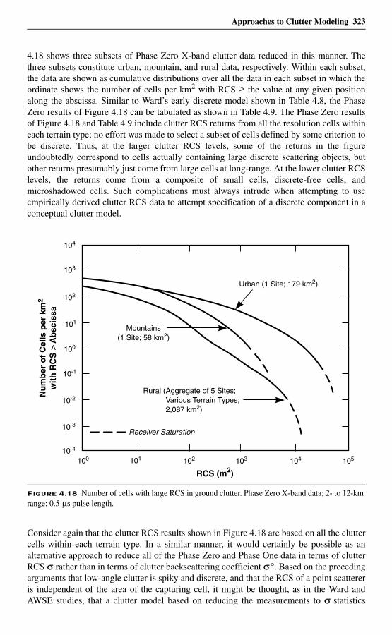
Approaches to Clutter Modeling 323

4.18 shows three subsets of Phase Zero X-band clutter data reduced in this manner. Thethree subsets constitute urban, mountain, and rural data, respectively. Within each subset,the data are shown as cumulative distributions over all the data in each subset in which theordinate shows the number of cells per km2 with RCS ≥ the value at any given positionalong the abscissa. Similar to Ward’s early discrete model shown in Table 4.8, the PhaseZero results of Figure 4.18 can be tabulated as shown in Table 4.9. The Phase Zero resultsof Figure 4.18 and Table 4.9 include clutter RCS returns from all the resolution cells withineach terrain type; no effort was made to select a subset of cells defined by some criterion tobe discrete. Thus, at the larger clutter RCS levels, some of the returns in the figureundoubtedly correspond to cells actually containing large discrete scattering objects, butother returns presumably just come from large cells at long-range. At the lower clutter RCSlevels, the returns come from a composite of small cells, discrete-free cells, andmicroshadowed cells. Such complications must always intrude when attempting to useempirically derived clutter RCS data to attempt specification of a discrete component in aconceptual clutter model.

Consider again that the clutter RCS results shown in Figure 4.18 are based on all the cluttercells within each terrain type. In a similar manner, it would certainly be possible as analternative approach to reduce all of the Phase Zero and Phase One data in terms of clutterRCS σ rather than in terms of clutter backscattering coefficient σ°. Based on the precedingarguments that low-angle clutter is spiky and discrete, and that the RCS of a point scattereris independent of the area of the capturing cell, it might be thought, as in the Ward andAWSE studies, that a clutter model based on reducing the measurements to σ statistics

Figure 4.18 Number of cells with large RCS in ground clutter. Phase Zero X-band data; 2- to 12-km range; 0.5-µs pulse length.

RCS (m2)

104

103

102

100

101

10-1

10-2

10-3

10-4

Nu

mb

er o

f C

ells

per

km

2

wit

h R

CS

A

bsc

issa

100 101 103 104 105102

Urban (1 Site; 179 km2)

Receiver Saturation

Mountains(1 Site; 58 km2)

Rural (Aggregate of 5 Sites; Various Terrain Types; 2,087 km2)

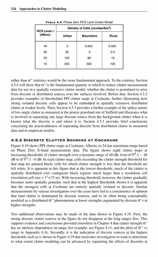
324 Approaches to Clutter Modeling

rather than σ° statistics would be the more fundamental approach. To the contrary, Section4.5.4 will show that σ° is the fundamental quantity to which to reduce clutter measurementdata for use in a spatially extensive clutter model, whether the clutter is postulated to arisefrom discrete or distributed sources over the surfaces involved. Before that, Section 4.5.2provides examples of thresholded PPI clutter maps at Cochrane, further illustrating howstrong isolated discrete cells appear to be embedded in spatially extensive distributedclutter at weaker levels. Then, Section 4.5.3 provides a further example of the spikey natureof low-angle clutter as measured at the prairie grassland site of Suffield and illustrates whatis involved in separating one large discrete source from the background clutter when it isknown what the discrete is and where it is. Section 4.5.5 provides brief conclusionsconcerning the practicableness of separating discrete from distributed clutter in measureddata and in empirical models.

4.5.2 Discrete Clutter Sources at CochraneFigure 4.19 shows PPI clutter maps at Cochrane, Alberta, to 24-km maximum range basedon Phase Zero X-band measurement data. The figure shows eight clutter maps atincreasing thresholds of clutter strength over a dynamic range of 40 dB, from σ°F4 ≥ − 48dB to σ°F4 ≥ –8 dB. In each clutter map, cells exceeding the clutter strength threshold forthat map are painted black; cells for which clutter strength is less than the threshold areleft white. It is apparent in this figure that at the lowest thresholds, much of the clutter isspatially distributed over contiguous black regions much larger than a resolution cell(resolution cell size = 1°×75 m). With increasing threshold, however, the clutter graduallybecomes more spatially granular, such that at the highest thresholds shown it is apparentthat the strongest cells at Cochrane are entirely spatially isolated or discrete. Similarmeasurements by various investigators over the years have led to a concurrence of opinionthat land clutter is dominated by discrete sources, and to its often being conceptuallymodeled as a distributed σ ° phenomenon at lower strengths augmented by discrete σ ’s athigher strengths.

Two additional observations may be made of the data shown in Figure 4.19. First, thestrong discrete clutter sources in the figure do not disappear at the long ranges first. Thissupports evidence and conclusions provided elsewhere in Chapter 4 that clutter strength σ°has no intrinsic dependence on range (for example, see Figure 4.11, and the plots of σ ° vsrange in Appendix 4.A). Secondly, it is the indication of discrete sources at the highestthresholds such as is shown in Figure 4.19 that motivates investigators to want to determineto what extent clutter modeling can be advanced by separating the effects of discretes at

Table 4.9 Phase Zero RCS Land Clutter Model

Density of Cells (number/km2)RCS Level σ

(dBsm) Urban Mountains Rural

40

30

20

10

3

30

100

300

0.004

3

80

300

0.004

0.3

10

100

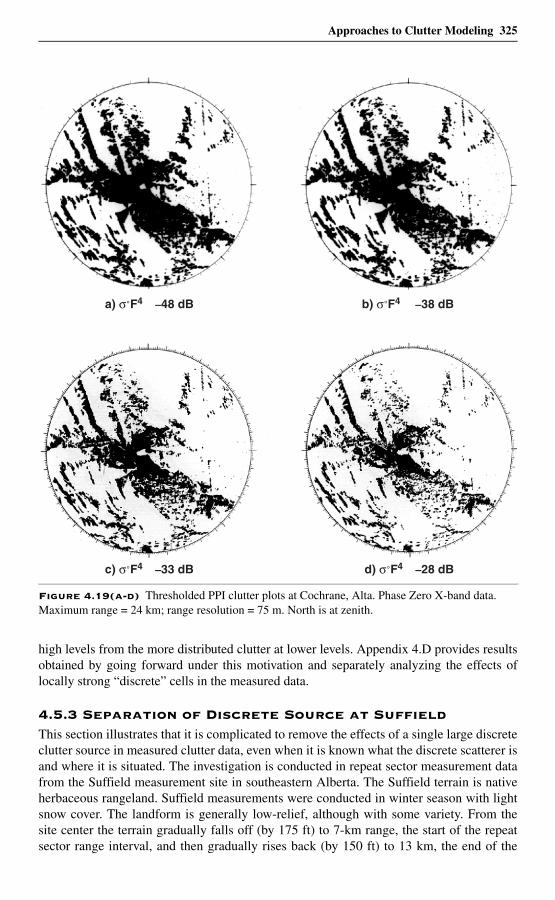
Approaches to Clutter Modeling 325

high levels from the more distributed clutter at lower levels. Appendix 4.D provides resultsobtained by going forward under this motivation and separately analyzing the effects oflocally strong “discrete” cells in the measured data.

4.5.3 Separation of Discrete Source at SuffieldThis section illustrates that it is complicated to remove the effects of a single large discreteclutter source in measured clutter data, even when it is known what the discrete scatterer isand where it is situated. The investigation is conducted in repeat sector measurement datafrom the Suffield measurement site in southeastern Alberta. The Suffield terrain is nativeherbaceous rangeland. Suffield measurements were conducted in winter season with lightsnow cover. The landform is generally low-relief, although with some variety. From thesite center the terrain gradually falls off (by 175 ft) to 7-km range, the start of the repeatsector range interval, and then gradually rises back (by 150 ft) to 13 km, the end of the

Figure 4.19(a-d) Thresholded PPI clutter plots at Cochrane, Alta. Phase Zero X-band data. Maximum range = 24 km; range resolution = 75 m. North is at zenith.

a) σ˚F4 –48 dB b) σ˚F4 –38 dB

c) σ˚F4 –33 dB d) σ˚F4 –28 dB

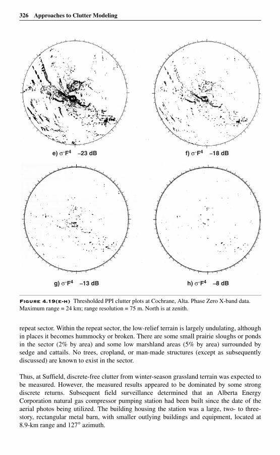
326 Approaches to Clutter Modeling

repeat sector. Within the repeat sector, the low-relief terrain is largely undulating, althoughin places it becomes hummocky or broken. There are some small prairie sloughs or pondsin the sector (2% by area) and some low marshland areas (5% by area) surrounded bysedge and cattails. No trees, cropland, or man-made structures (except as subsequentlydiscussed) are known to exist in the sector.

Thus, at Suffield, discrete-free clutter from winter-season grassland terrain was expected tobe measured. However, the measured results appeared to be dominated by some strongdiscrete returns. Subsequent field surveillance determined that an Alberta EnergyCorporation natural gas compressor pumping station had been built since the date of theaerial photos being utilized. The building housing the station was a large, two- to three-story, rectangular metal barn, with smaller outlying buildings and equipment, located at8.9-km range and 127° azimuth.

Figure 4.19(e-h) Thresholded PPI clutter plots at Cochrane, Alta. Phase Zero X-band data. Maximum range = 24 km; range resolution = 75 m. North is at zenith.

e) σ˚F4 –23 dB f) σ˚F4 –18 dB

g) σ˚F4 –13 dB h) σ˚F4 –8 dB

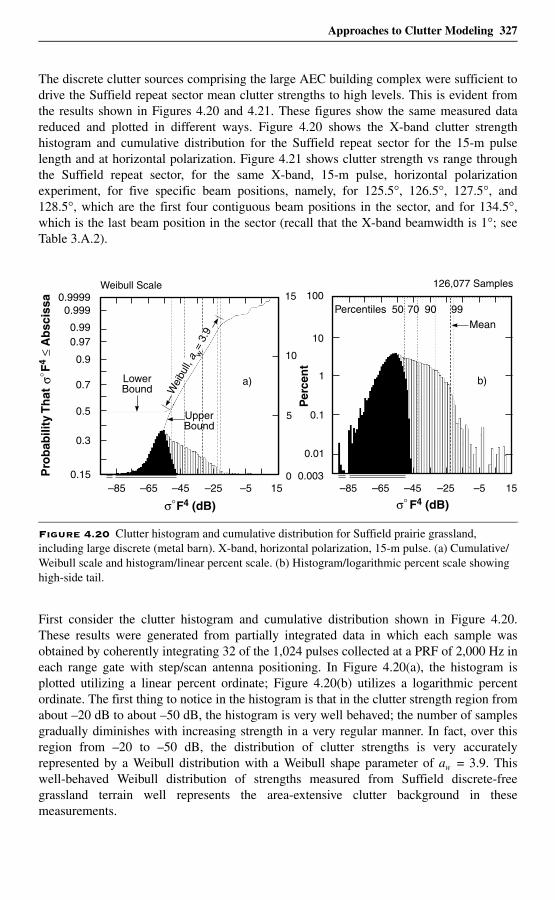
Approaches to Clutter Modeling 327

The discrete clutter sources comprising the large AEC building complex were sufficient todrive the Suffield repeat sector mean clutter strengths to high levels. This is evident fromthe results shown in Figures 4.20 and 4.21. These figures show the same measured datareduced and plotted in different ways. Figure 4.20 shows the X-band clutter strengthhistogram and cumulative distribution for the Suffield repeat sector for the 15-m pulselength and at horizontal polarization. Figure 4.21 shows clutter strength vs range throughthe Suffield repeat sector, for the same X-band, 15-m pulse, horizontal polarizationexperiment, for five specific beam positions, namely, for 125.5°, 126.5°, 127.5°, and128.5°, which are the first four contiguous beam positions in the sector, and for 134.5°,which is the last beam position in the sector (recall that the X-band beamwidth is 1°; seeTable 3.A.2).

First consider the clutter histogram and cumulative distribution shown in Figure 4.20.These results were generated from partially integrated data in which each sample wasobtained by coherently integrating 32 of the 1,024 pulses collected at a PRF of 2,000 Hz ineach range gate with step/scan antenna positioning. In Figure 4.20(a), the histogram isplotted utilizing a linear percent ordinate; Figure 4.20(b) utilizes a logarithmic percentordinate. The first thing to notice in the histogram is that in the clutter strength region fromabout –20 dB to about –50 dB, the histogram is very well behaved; the number of samplesgradually diminishes with increasing strength in a very regular manner. In fact, over thisregion from –20 to –50 dB, the distribution of clutter strengths is very accuratelyrepresented by a Weibull distribution with a Weibull shape parameter of aw = 3.9. Thiswell-behaved Weibull distribution of strengths measured from Suffield discrete-freegrassland terrain well represents the area-extensive clutter background in thesemeasurements.

Figure 4.20 Clutter histogram and cumulative distribution for Suffield prairie grassland, including large discrete (metal barn). X-band, horizontal polarization, 15-m pulse. (a) Cumulative/Weibull scale and histogram/linear percent scale. (b) Histogram/logarithmic percent scale showing high-side tail.

Per

cen

t15

10

5

a)LowerBound

Weibull Scale

UpperBound

0

F4 (dB)

Pro

bab

ility

Th

at

F4

A

bsc

issa

–85 –65 –45 –250.15

0.3

0.5

0.7

0.9

0.970.99

0.9990.9999

–5 15

Percentiles 50 70 90 99Mean

100

10

1

0.1

b)

0.01

0.003–85

F4 (dB)–65 –45 –25 –5 15

126,077 Samples

Wei

bull,

a w=

3.9

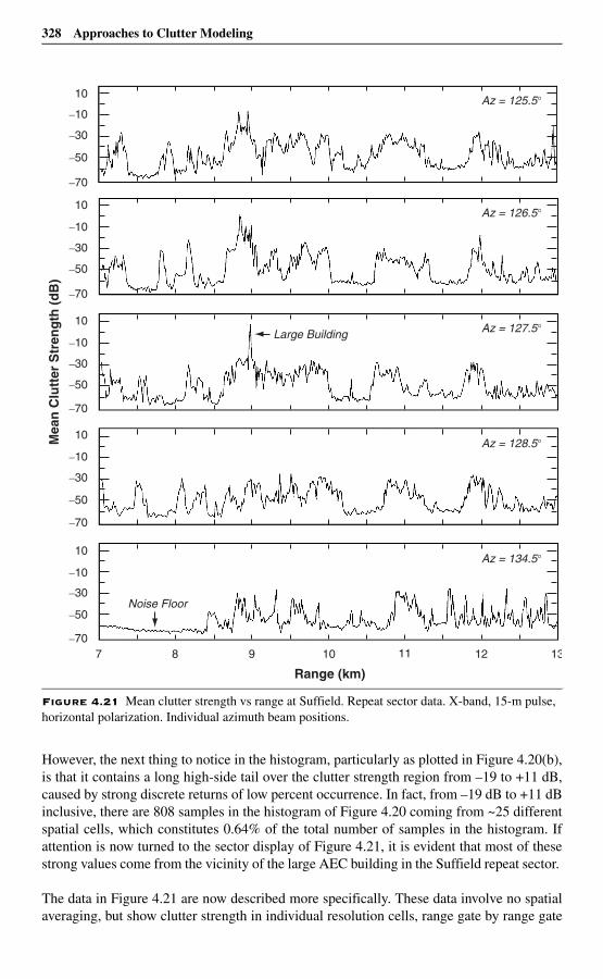
328 Approaches to Clutter Modeling

However, the next thing to notice in the histogram, particularly as plotted in Figure 4.20(b),is that it contains a long high-side tail over the clutter strength region from –19 to +11 dB,caused by strong discrete returns of low percent occurrence. In fact, from –19 dB to +11 dBinclusive, there are 808 samples in the histogram of Figure 4.20 coming from ~25 differentspatial cells, which constitutes 0.64% of the total number of samples in the histogram. Ifattention is now turned to the sector display of Figure 4.21, it is evident that most of thesestrong values come from the vicinity of the large AEC building in the Suffield repeat sector.

The data in Figure 4.21 are now described more specifically. These data involve no spatialaveraging, but show clutter strength in individual resolution cells, range gate by range gate

Figure 4.21 Mean clutter strength vs range at Suffield. Repeat sector data. X-band, 15-m pulse, horizontal polarization. Individual azimuth beam positions.

–10

10

–30

–50

–70

–10

10

–30

–50

–70

–10

10

–30

–50

–70

–10

10

–30

–50

–70

–10

10

–30

–50

–707 8 9 10 11 12 13

Az = 125.5°

Az = 126.5°

Az = 127.5°

Az = 128.5°

Az = 134.5°

Mea

n C

lutt

er S

tren

gth

(d

B)

Range (km)

Large Building

Noise Floor

Approaches to Clutter Modeling 329

and beam position by beam position. In each resolution cell, the clutter strength shown isthe temporal mean strength resulting from averaging 32 samples, each of which is acoherent average of 32 pulses recorded at a PRF of 2,000 Hz. Generally, Figure 4.21indicates that the clutter from this Suffield grassland terrain is of a very spiky nature, with30-dB fluctuations common, as individual cells drop into and out of direct visibility at thelow 0.3-deg depression angle involved. These data are a good example of the statisticalnature of low-angle clutter, even from what is relatively homogeneous, discrete-freegrassland terrain (i.e., not constant σ° or a tight Rayleigh process). Most of these clutterreturns vary over the range from –20 to –50 or –60 dB. The major exception to this range ofvariation in the data of Figure 4.21 is the set of returns of strength >> –20 dB from cells inthe near vicinity of the AEC building in the range interval from 8.8 to 9.0 km and atazimuths from 125.5° to 127.5°. For example, at the 127.5° azimuth position there is astrong specular flash directly from this building that raises the clutter return 30 dB or moreabove the envelope of the peaks in other cells not near the building. Although in thefollowing beam position (i.e., 128.5°) no indication of the building remains, in the twopreceding beam positions there is significant evidence of the building and associateddiscretes at levels > –20 dB spread over a number of range gates. Altogether, in these datathere are 435 samples of strength ≥ –13 dB from the vicinity of the AEC building, which, ifdeleted, reduce the mean strength in the histogram of Figure 4.20 from –22.6 to –34.9 dB.Note that the general statistical nature of the grassland clutter at 134.5°, the final beamposition in the sector, is relatively similar in range of fluctuation to that 6° earlier (i.e., at128.5°) except over the region from 7 to 8.5 km. This region is shadowed terrain at thenoise floor, where the noise level decreases with increasing range because r4 sensitivity-time-control (STC) attenuation was used in the experiment. The 5-dB discrete-findingalgorithm utilized in Appendix 4.D clearly would specify a number of cells in Figure 4.21as being “discrete,” i.e., as being 5 dB stronger than their neighbors, even though noobvious point-like discrete physical scattering sources other than the AEC building areknown to exist in the Suffield repeat sector.

Thus, the data of Figures 4.20 and 4.21 indicate that a more appropriate value of X-bandmean clutter strength (at 15-m pulse length, horizontal polarization) to represent discrete-free Suffield grassland is –34.9 dB, not the –22.6 dB value actually measured there anddriven to be so large by the presence of the AEC building. Next, similar adjustments toSuffield repeat sector mean clutter strengths are performed in other bands. These are done atlow resolution (i.e., 150-m pulse length). The low resolution data are more clear-cut as towhich samples come from the AEC building. Thus, in the L-band (150-m pulse, horizontalpolarization) data there are four cells at σ°F4 levels of –4, –8, –16, and –17 dB providingsamples (32 each) from the AEC building. When the samples from these four cells areremoved from the measured histogram, the mean strength of the histogram drops from –25.0to –39.9 dB. Similarly in the other bands (at 150-m pulse length, horizontal polarization), itis found that mean strengths adjust as follows: at X-band, from –21.7 to –33.9 dB; at S-band,from –25.3 to –43.2 dB; at L-band, from –25.0 to –39.9 dB; at UHF, from –36.8 to –40.3 dB;and at VHF, from –51.3 to –51.7 dB.

These adjusted Suffield mean clutter strengths (adjusted to be representative of grasslandwithout the large AEC building discrete clutter source) are now compared with thegrassland site of Vananda East which has similar landform (i.e., 3–5) but at which a higherdepression angle occurred. This comparison is made at 150-m pulse length and horizontalpolarization. At UHF, L-, and S-band, the adjusted Suffield values are remarkably close to

330 Approaches to Clutter Modeling

Vananda East values (the values are, for Suffield and Vananda East, respectively: at UHF,–40.3 dB vs –38.9 dB; at L-band, –39.9 dB vs –39.5 dB; at S-band, –43.2 dB vs –38.1dB). Furthermore, in these three bands at both these grassland sites, mean clutter strengthsare remarkably invariant with frequency at or near the –40-db level. These –40-db levelsare good estimates of mean clutter strength in these bands for canonical discrete-freegrassland, and therefore are what would be assigned as mean strengths to Weibulldistributions for representing an area-extensive distributed clutter background.

At VHF, although Vananda East mean clutter strength holds near the –40-db level (viz., –41.7dB), adjusted Suffield mean clutter strength drops to –51.7 dB (i.e., 10 dB weaker thanVananda East). This lower Suffield value is caused by VHF multipath loss from the hillslopelocal to the antenna at Suffield (see Appendix 3.B, Section 3.B.2), which does not occur forthe high-bluff site at Vananda East. Note that, at VHF, the adjusted Suffield mean strength isonly 0.4 dB weaker than the unadjusted value. This is because at VHF the cells containingthe AEC building, although 25 to 30 dB stronger than surrounding cells, were 5 dB weakerthan some cells at longer range which were strong due to multipath enhancement. Thisresulted in the mean clutter strength, dominated by these strong long-range cells,coincidentally being about equal to the strength of the cells containing the AEC building, sowhether the AEC cells are included or not has little effect on mean clutter strength at VHF.

At X-band, the Vananda East mean clutter strength abruptly rises from the –40-db level inlower bands to –27.7 dB. This effect is described elsewhere in this book (viz., see Sections3.4.1.5, 3.4.2, and 5.4.7.2). The adjusted Suffield X-band mean clutter strength also abruptlyrises from –40 dB, but to –33.9 dB, a level 6 dB weaker than measured for grassland atVananda East but still 11 dB stronger than measured for grassland at Big Grass Marsh.

The repeat sector values of mean clutter strength at Suffield, adjusted to be applicable torelatively discrete-free grassland by removal of cells containing the AEC building, are thusunderstandable and provide additional information within the context of the other discrete-freegrassland sites, Vananda East (same 3–5 landform as Suffield) and Big Grass Marsh (landform= 1, level). The depression angle at Suffield, 0.3 deg, is intermediate between the depressionangle at Big Grass Marsh, 0.2 deg, and that at Vananda East, 1.0 deg. As a result, at VHF andX-band, adjusted values of Suffield mean clutter strength for grassland lie intermediatebetween those at Big Grass Marsh and at Vananda East. At UHF, L-, and S-band, adjustedvalues of Suffield mean clutter strength are very nearly equivalent to those at Vananda East.

These Suffield results indicate that, in the separation of returns from a known discrete cluttersource (viz., large building) in the measurement data, it is not so simple as the finding of asingle large value of RCS in a single cell, but instead what is found are multiple returns fromthe building varying over orders of magnitude from a number of small contiguous cells, eachof which partially intersects the building. This technique of separately dealing with largeman-made discretes in the clutter data is usually much more demanding than at Suffieldbecause usually many such sources exist in open terrain (e.g., farmland).

4.5.4 σ vs σ ° NormalizationSection 4.5.1 raised the idea that a conceptual ground clutter model comprising (1) a σ °component for area-extensive background clutter that is distributed over all cells,augmented by (2) a σ component for discrete clutter arising from large point sourcesoccupying a relatively small proportion of cells, is intuitively satisfying at low or high

Approaches to Clutter Modeling 331

angle. However, Sections 4.5.1–4.5.3 further showed that in working with measured low-angle clutter data, which unlike clutter data at higher angles is spiky throughout, it is notreadily feasible to separate a distributed σ ° component known a priori to arise fromphysically extended surfaces from a discrete σ component known a priori to arise fromphysical point objects. Nevertheless, and also as illustrated in Section 4.5.1, one maychoose to reduce all the measured clutter data either to clutter RCS σ per resolution cell orto normalized clutter RCS or backscattering coefficient σ° (where σ ° = σ /A, A = cell area= r •∆r • ∆θ; see Figure 2.4). Section 4.5.1 showed that the predilection of some previousinvestigators was to reduce all the measured clutter data to σ , on the basis that the strongerelements of low-angle clutter were spatially isolated or point-like (see Figure 4.19), andthat the RCS σ of a point source is the fundamental quantity independent of the size of thecapturing cell, as opposed to σ° which depends on the size of the capturing cell. Is it just amatter of subjective choice or preference on the part of the investigator, or do substantivereasons exist for making either σ or σ ° the preferable choice to which to reduce measuredlow-angle clutter data?

For us to begin to address this question, reference is first made to the results of Section3.5.3 in Chapter 3 showing that in measured repeat sector clutter data, the mean value of theclutter coefficient is essentially independent of cell area or spatial resolution (see Table3.10, small differences with pulse length in all five bands). Independence of mean strengthon cell area is necessary for the concept of density function to be true. It is true in themeasured data, irrespective of whether descriptive adjectives like “discrete” or“distributed” are associated with the measured data, and also irrespective of whether thenature of the measured clutter is very uniform or very spiky. Thus, as described elsewherethroughout this book, the fact that is independent of cell area is fundamentallyimportant to the structure of the modeling information presented. In contrast, if all theclutter measurement data are reduced to σ rather than σ°, the mean value of clutter RCS σover a spatial region is dependent on cell area, as σ = . Clutter modeling informationpresented in terms of σ rather than σ° would require the mean values σ of clutter amplitudedistributions to be shown as functions of resolution. In other words, σ is not as fundamentala quantity for specifying clutter amplitudes over extended spatial regions as is σ°.

Beyond this, care must be taken not to read too much into the fact that is independent ofcell area A. For example, it is easy to presume that this fact indicates that low-angle clutteris essentially not point-like but from extended surfaces—however, this is an incorrectassumption. What is indicated is that spiky clutter from discrete sources occurs distributedover surfaces; i.e., that in low-angle clutter, both adjectives apply—clutter is both“discrete” and “distributed.”

It is easy to appreciate that mean clutter cross section increases linearly with cell area (i.e.,σ = ) in area-extensive clutter. But how does this observation square with the fact thatin clutter arising from point sources, the more basic quantity for the cell capturing the cluttersource is its RCS σ which is independent of the capturing cell size? A simple example maybe illuminating in this regard. Imagine the existence of a hypothetical clutter spatial field inwhich each cell contains a single point discrete of σ = X. One might choose to characterizethis clutter in terms of its mean clutter RCS such that σ = X. Now suppose the resolution ofthe radar to change so as to either increase or decrease by a factor of 10. If the resolutionincreases, one-tenth of the cells will capture a discrete and have σ = X; the other nine-tenthsof cells will miss capturing a discrete and will have σ = 0. Thus if the resolution increases by

σ°

σ°

σ° A⋅

σ°

σ° A⋅

332 Approaches to Clutter Modeling

a factor of 10, σ = X/10. If, on the other hand, the resolution decreases by a factor of 10, eachcell captures 10 discretes and (under the assumption that the 10 discretes combine as apower-additive process) σ = 10X. Thus even in this hypothetical discrete clutter field, meanclutter RCS σ varies linearly with cell area similarly as it does in the actual measured data.That is, σ is not an invariant irreducible quantity suitable for basing a model upon.

Next consider the hypothetical clutter spatial field in σ° space. At the original rangeresolution, say 150 m, the σ° of each cell (each cell containing a single discrete of RCS =X) is X/( ). Next, allow the range resolution to increase by a factor of 10, to15 m. Each discrete-capturing 15-m cell still provides RCS = X, and the σ° of eachdiscrete-capturing cell rises by a factor of 10 to σ° = X/( ). But in the regionaround each discrete-capturing cell, there are now nine empty cells with σ° = 0. Thus themean value of σ° over each 10-cell region is = [X/( )]/10 which is the samevalue of σ° as measured with the 150-m cell. Similarly, if range resolution is allowed todecrease from its original 150-m value by a factor of 10 to 1500 m, each cell captures 10discretes; so =10X/( ) which is also the same value of as measuredwith the 150-m cell.

Thus in considering ground clutter, all possibilities of cells on the ground must be specifieddepending on resolution, not just cells capturing single discretes, but including possibilitiesof cells capturing more than one discrete and cells capturing no discretes. This is the pointthat is missed when intuition incorrectly suggests that σ is a more basic quantity than σ° forcharacterizing discrete clutter. Certainly, in a backscatter measurement of any single pointobject in which concern is only with the cell containing the object and not the surroundingempty cells, the appropriate characterization of the object is by its RCS σ.

This hypothetical situation of a clutter spatial field in which at intermediate resolution eachcell contains a single discrete clutter source of RCS = X is handled by a σ° clutter model asfollows. At all three resolutions, the mean value of clutter coefficient remains constant,invariant with cell size (as in the modeling information in this book). The different σ°distributions for the three variations in range resolution are theoretically handled throughspecification of differently shaped distributions for the three resolutions, but with foreach distribution remaining unchanged (also as occurs in the modeling information in thisbook). Thus in these hypothetical situations, for the mid-size cell, the shape of thedistribution is an impulse allowing no variation in σ°; for the small cell, the shape of thedistribution is such as to define a two-impulse bipolar distribution with nine-tenths of theσ° values equal to zero and one-tenth equal to X/( ); and for the large cell, theshape of the distribution is such as to allow the variability associated with 10 interferingscatterers within the cell. For the actual measured clutter data, as opposed to the abovehypothetical construct, such extreme shapes of distributions are unnecessary; the Weibulldistribution of constant mean strength and varying shape parameter aw is sufficient tohandle the actual variations in shape that occur with changing resolution in the actualmeasured data.

The above reasoning indicates that when concern is with returns from all the cells defininga surface, the correct way to empirically characterize the phenomenon is to reduce themeasured data to σ°, even though each return in itself may arise from a point source. Is thisreasoning supported by the observed behavior of the actual measured clutter data? Consideragain that since is independent of cell area, σ = must increase linearly with

r 150 ∆θ⋅ ⋅

r 15 ∆ θ⋅ ⋅

σ ° r 15 ∆θ⋅ ⋅

σ ° r 1500 ∆θ⋅ ⋅ σ °

σ °

σ °

r 15 ∆ θ⋅ ⋅

σ °w

σ° σ° A⋅

Approaches to Clutter Modeling 333

increasing cell area. Thus in observed clutter data, if range is allowed to increase from 1 kmto, say, 64 km (that is, by six factors of 2), cell area doubles with each factor of 2 increase inrange leading to the expectation that clutter RCS would increase by 18 dB over this range,certainly enough to show a noticeable trend in measured data. That is, larger cells at longerranges capture more discretes and provide larger cross sections. But in the σ° vs rangeresults shown in this book, for example in the sector displays of Appendix 4.A or in thethresholded PPI displays of Figure 4.19, no strong trends of σ° vs range are observed,indicating that σ° is indeed the appropriate irreducible quantity upon which to base aclutter model. In all observations, σ° within visible clutter regions (although fluctuatingstrongly from cell to cell) neither increases nor decreases significantly with range, butremains as a fundamental quantity with range effects properly normalized out.

It is apparent from the preceding discussion that σ°, as opposed to σ , is the morefundamental quantity to which to reduce measured low-angle clutter data, despite the factthat low-angle clutter is an essentially spiky phenomenon arising from a sea of discreteclutter sources. A clutter model based on reducing all measured returns to σ is notcompletely reduced; such a model must include σ depending on resolution as an extracomplicating dimension that is not necessary in a model based on σ°. This fact leads to theclutter data in this book being reduced to σ° as the most basic characteristic of a distributedphenomenon, despite the fact that what is distributed are discrete clutter sources.

4.5.5 ConclusionsThe idea behind separating discrete clutter sources in measured clutter data is that objectslike water towers act as contaminants in what would otherwise be a statistically well-behaved area-extensive clutter background from the land surface itself, and that a betterclutter model results if RCS values of strong discretes are added in a separate σ process tothe basic distributed σ ° component representing the background clutter. This idea hassome validity at higher angles of illumination typical of airborne radar platforms. At thelow angles of illumination of ground-based radars, the focus of the idea tends to dissipatefor several reasons. First, low-angle clutter is spiky throughout; removal of the largestspikes still leaves a spiky background. Second, it is not possible to deterministicallyseparate clutter arising from point objects from clutter arising from extended surfaces inthe measured data. Many spikes occur only because of vicissitudes of visibility andshadowing compounded by extreme propagation variations at very low angles ofillumination. Little correlation exists between locally strong clutter returns and knownpoint objects on the ground. Third, even though low-angle clutter appears to arise from asea of discretes, the proper way to reduce the data is to the normalized clutter coefficientσ °, as opposed to radar cross section σ , irrespective of whether one is examining so-called“distributed” or “discrete” components.

Given these qualifications, if we continue to wish to examine the usefulness of separatelyanalyzing and modeling strong clutter as an overlay to the general clutter background, it isnecessary to fall back to a position in which locally strong cells are specified a posterioriin the measured clutter data as opposed to their a priori specification as the returns fromknown point objects.

In so doing, the initial premise has changed. Rather than removing and separately modelingthe returns from known point discretes such as water towers, the question now being posedis if it is useful to model the total clutter distribution from a given spatial region as two

334 Approaches to Clutter Modeling

components, one consisting of the locally strong clutter cells resulting from passing aspatial filter over the data and the other consisting of the residual clutter cells which failedto pass the filter. That is, is it useful to set a threshold so as to separate locally strong σ°from weaker surrounding σ°. The potential benefit of such a procedure hinges on thepossibility of there being a difference in kind, not just degree, in the two distributions (eventhough each consists of spiky returns) such that each might be of a relatively simple shape,whereas their combination is of a more complex shape. Note that both components arebroad distributions consisting of spiky returns of strengths differing by orders ofmagnitude, with the major differences being that the so-called “discrete” componentconsists of locally strong spiky returns and the so-called “background” component consistsof the weaker neighboring spiky returns. Further, note that there is no benefit and indeedneedless added complexity in moving to σ space to characterize the locally strong or so-called “discrete” component.

The modeling of clutter based on the two-distribution approach allows the possibility ofassigning two random variates to each clutter cell with the resulting total σ° being thephasor addition of the two components. This approach models “discrete” clutter returnsstatistically rather than attempting to deterministically specify returns from known pointtargets on the landscape. Appendix 4.D shows results obtained from separating clutter intotwo σ° components in this manner. The main approach of this book, however, is tocharacterize the total clutter from a given spatial region as a single Weibull distribution,where the broad extent of the Weibull distribution usually satisfactorily represents themeasured distribution, capturing the occasional strong returns from discrete sources atappropriate probabilities of occurrence. The clutter modeling information provided inChapter 5 and elsewhere (except in Appendix 4.D) in this book is based on the single-distribution approach involving the assignment of a single random variate to representclutter strength in each resolution cell.

4.6 Temporal Statistics, Spectra, and CorrelationFor many years, in radars of low spatial resolution, the in-phase and quadraturecomponents of the spatially varying ground clutter signal were considered to bedistributed as Gaussian probability density functions, resulting in the signal amplitudebeing Rayleigh distributed (see, for example [12], Section 10.2). In modern radar systems,operating at low grazing angles and with resolution capabilities high enough to resolve thesurface structure, the statistics of the clutter have been observed to strongly deviate fromGaussianity [13–19]. The clutter is spikier than if it were Gaussian, and the spikes areprocessed by the radar detector as targets, with increased false-alarm rate. Until now,Chapter 4 and the preceding chapters of this book have been primarily concerned with thecharacterizations and prediction of the highly non-Gaussian clutter amplitude statisticsresulting from cell-to-cell spatial variations in ground clutter signals.

Windblown ground clutter Doppler spectra also in early years were, like the amplitudedistributions, erroneously thought to be of Gaussian shape [20–22]. The correctunderstanding of ground clutter and the accurate modeling of its non-Gaussian behavior,both in the spatial amplitude distribution and in the Doppler spectrum, are problems offundamental interest to the radar community for successful radar design and performanceprediction. The subject now widens to include temporal variations in the received clutter

Approaches to Clutter Modeling 335

signals returned from particular spatial cells. Important attributes of temporal statistics are(1) temporal amplitude statistics, (2) spectral characteristics, and (3) correlation times.Correlation distance in the ground clutter spatial process is also discussed. Improvedknowledge of these various additional attributes of ground clutter, in addition to its spatialamplitude statistics, is required in the demanding specialized design of modern signalprocessors required to detect, track, and otherwise operate against ever-smaller radartargets in ground clutter backgrounds. For example, the spectral characteristics of clutterdetermine the design of moving target indicator (MTI) or space-time adaptive processors(STAP) [23, 24], and the amplitude statistics of clutter affect the design of constant-false-alarm rate (CFAR) processors (see e.g., [12, p. 306; 25]).

Results concerning these additional important attributes of low-angle ground clutter areprovided in Section 4.6 at a first or introductory level of analysis. More in-depth analyses ofthese attributes based on the Phase One clutter data are available elsewhere [26–31]. Theyshow that the temporal and spatial domains of ground clutter are interrelated. However, inthe specification of the spatial clutter amplitude statistics which is a principal focus of thisbook, each individual spatial clutter amplitude so specified may be regarded as the meanlevel of a temporal process in a given spatial cell. Subsequently, Chapter 6 takes up thesubject of the modeling of windblown ground clutter spectral shape as a second principalfocus of this book.

4.6.1 Temporal StatisticsFigure 4.22 presents information describing the relative frequency of occurrence of temporalamplitude statistics between cells with Rayleigh (i.e., windblown foliage) and Ricean (i.e.,fixed discretes embedded in foliage) statistics. Ricean statistics describe ground cluttertemporal variations from a fixed spatial cell quite accurately as the return of a dominantsteady reflector or fixed discrete in a varying background [22, 32]. Rayleigh statistics are alimiting case of Ricean statistics with steady signal equal to zero. The quantity m2 in theRicean distribution as introduced by Goldstein [22] is the ratio of steady to random averagepower, or, in other words, the dominant-to-Rayleigh reflector ratio. The ratio of standarddeviation-to-mean (sd/mean) in the Ricean process is related to m2 as sd/mean = [(1 + 2 m2)/ (1 + m2)2]0.5 ≅ /m for m2 >> 1.

The data in Figure 4.22 indicate that, over a population of 988 relatively strong clutter cellsselected from three rural sites, more than 40% of the cells are Rayleigh (i.e., have ratios ofstandard deviation-to-mean = 0 dB), and the remainder are generally Ricean (i.e., have ratiosof standard deviation-to-mean < 0 dB), with increasingly strong Ricean cells occurring lessfrequently. For example, Figure 4.22 shows that 1% of cells are strongly enough dominatedby fixed discretes to have a dominant-to-Rayleigh reflector ratio as high as 50. The reasonthat 40% of the clutter cells in the figure contain only windblown foliage with dominant-to-Rayleigh reflector ratio equal to zero is that there are some trees on these farmlandlandscapes. Where trees occur, even at relatively low incidence of occurrence, they tend todominate as strong clutter sources (see Chapter 2, Section 2.4.2.5).

4.6.2 Spectral Characteristics For Rayleigh cells containing windblown trees, the wind-induced motion causes Doppler-shifted energy in the power spectra of the received temporal signals. Figure 4.23 showstwo examples of windblown ground clutter spectral results, each computed from a PhaseOne X-band long-time-dwell experiment measured from the same forested cell at 2.6-km

2

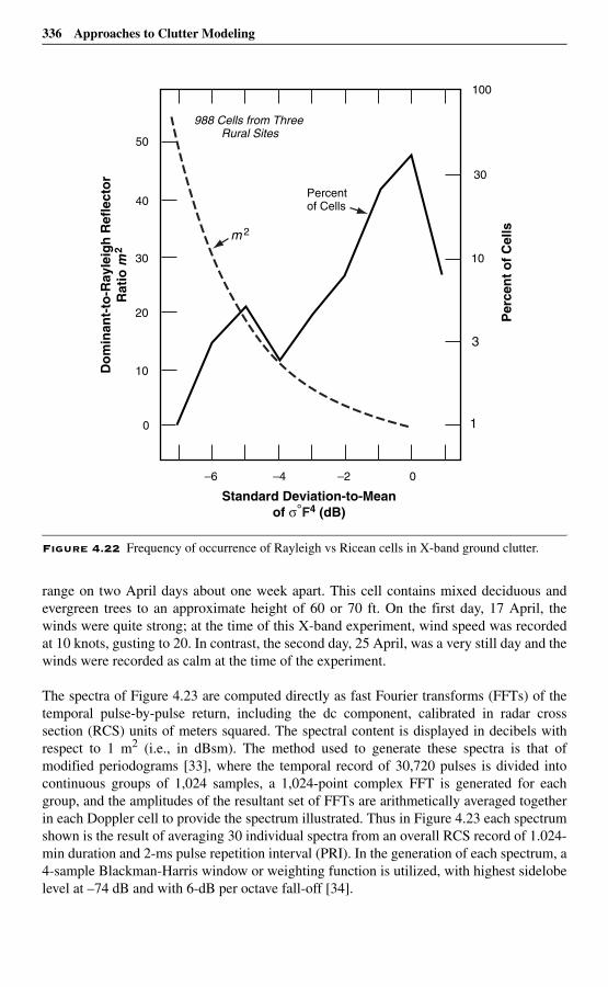
336 Approaches to Clutter Modeling

range on two April days about one week apart. This cell contains mixed deciduous andevergreen trees to an approximate height of 60 or 70 ft. On the first day, 17 April, thewinds were quite strong; at the time of this X-band experiment, wind speed was recordedat 10 knots, gusting to 20. In contrast, the second day, 25 April, was a very still day and thewinds were recorded as calm at the time of the experiment.

The spectra of Figure 4.23 are computed directly as fast Fourier transforms (FFTs) of thetemporal pulse-by-pulse return, including the dc component, calibrated in radar crosssection (RCS) units of meters squared. The spectral content is displayed in decibels withrespect to 1 m2 (i.e., in dBsm). The method used to generate these spectra is that ofmodified periodograms [33], where the temporal record of 30,720 pulses is divided intocontinuous groups of 1,024 samples, a 1,024-point complex FFT is generated for eachgroup, and the amplitudes of the resultant set of FFTs are arithmetically averaged togetherin each Doppler cell to provide the spectrum illustrated. Thus in Figure 4.23 each spectrumshown is the result of averaging 30 individual spectra from an overall RCS record of 1.024-min duration and 2-ms pulse repetition interval (PRI). In the generation of each spectrum, a4-sample Blackman-Harris window or weighting function is utilized, with highest sidelobelevel at –74 dB and with 6-dB per octave fall-off [34].

Figure 4.22 Frequency of occurrence of Rayleigh vs Ricean cells in X-band ground clutter.

–6 –4 –2 0

100

30

10

3

1

50

40

30

20

10

0

Standard Deviation-to-Meanof σ°F4 (dB)

Per

cen

t o

f C

ells

Do

min

ant-

to-R

ayle

igh

Ref

lect

or

Rat

io m

2988 Cells from Three

Rural Sites

m 2

Percentof Cells

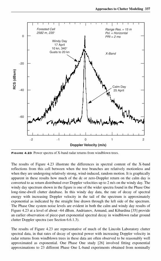
Approaches to Clutter Modeling 337

The results of Figure 4.23 illustrate the differences in spectral content of the X-bandreflections from this cell between when the tree branches are relatively motionless andwhen they are undergoing relatively strong, wind-induced, random motion. It is graphicallyapparent in these results how much of the dc or zero-Doppler return on the calm day isconverted to ac return distributed over Doppler velocities up to 2 m/s on the windy day. Thewindy day spectrum shown in the figure is one of the wider spectra found in the Phase Onelong-time-dwell clutter database. In this windy day data, the rate of decay of spectralenergy with increasing Doppler velocity in the tail of the spectrum is approximatelyexponential as indicated by the straight line drawn through the left side of the spectrum.The Phase One system noise levels are evident in both the calm and windy day results ofFigure 4.23 at a level of about –64 dBsm. Andrianov, Armand, and Kibardina [35] providean earlier observation of piece-part exponential spectral decay in windblown radar groundclutter Doppler spectra (see Section 6.6.1.3).

The results of Figure 4.23 are representative of much of the Lincoln Laboratory clutterspectral data, in that rates of decay of spectral power with increasing Doppler velocity inradar returns from windblown trees in these data are often observed to be reasonably wellapproximated as exponential. One Phase One study [26] involved fitting exponentialapproximations to 23 different Phase One L-band experiments obtained from nominally

Figure 4.23 Power spectra of X-band radar returns from windblown trees.

–60

–40

–20

0

RC

S (

dB

sm)

Doppler Velocity (m/s)

–2 –1 0 1 2

Forested Cell2582 m, 235°

Windy Day17 April

10 kn, 340°Gusts to 20 kn

Range Res. = 15 mPol. = HorizontalPRI = 2 ms

X-Band

Calm Day25 April

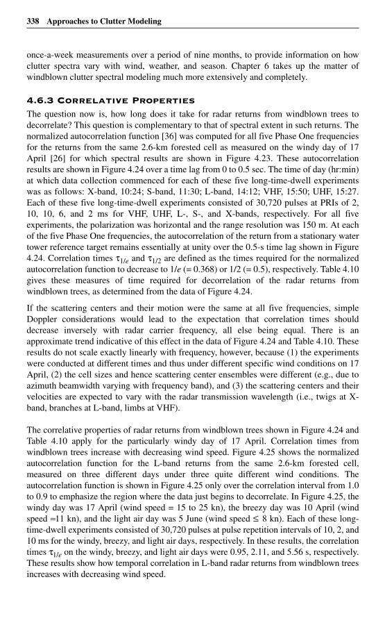
338 Approaches to Clutter Modeling

once-a-week measurements over a period of nine months, to provide information on howclutter spectra vary with wind, weather, and season. Chapter 6 takes up the matter ofwindblown clutter spectral modeling much more extensively and completely.

4.6.3 Correlative PropertiesThe question now is, how long does it take for radar returns from windblown trees todecorrelate? This question is complementary to that of spectral extent in such returns. Thenormalized autocorrelation function [36] was computed for all five Phase One frequenciesfor the returns from the same 2.6-km forested cell as measured on the windy day of 17April [26] for which spectral results are shown in Figure 4.23. These autocorrelationresults are shown in Figure 4.24 over a time lag from 0 to 0.5 sec. The time of day (hr:min)at which data collection commenced for each of these five long-time-dwell experimentswas as follows: X-band, 10:24; S-band, 11:30; L-band, 14:12; VHF, 15:50; UHF, 15:27.Each of these five long-time-dwell experiments consisted of 30,720 pulses at PRIs of 2,10, 10, 6, and 2 ms for VHF, UHF, L-, S-, and X-bands, respectively. For all fiveexperiments, the polarization was horizontal and the range resolution was 150 m. At eachof the five Phase One frequencies, the autocorrelation of the return from a stationary watertower reference target remains essentially at unity over the 0.5-s time lag shown in Figure4.24. Correlation times τ1/e and τ1/2 are defined as the times required for the normalizedautocorrelation function to decrease to 1/e (= 0.368) or 1/2 (= 0.5), respectively. Table 4.10gives these measures of time required for decorrelation of the radar returns fromwindblown trees, as determined from the data of Figure 4.24.

If the scattering centers and their motion were the same at all five frequencies, simpleDoppler considerations would lead to the expectation that correlation times shoulddecrease inversely with radar carrier frequency, all else being equal. There is anapproximate trend indicative of this effect in the data of Figure 4.24 and Table 4.10. Theseresults do not scale exactly linearly with frequency, however, because (1) the experimentswere conducted at different times and thus under different specific wind conditions on 17April, (2) the cell sizes and hence scattering center ensembles were different (e.g., due toazimuth beamwidth varying with frequency band), and (3) the scattering centers and theirvelocities are expected to vary with the radar transmission wavelength (i.e., twigs at X-band, branches at L-band, limbs at VHF).

The correlative properties of radar returns from windblown trees shown in Figure 4.24 andTable 4.10 apply for the particularly windy day of 17 April. Correlation times fromwindblown trees increase with decreasing wind speed. Figure 4.25 shows the normalizedautocorrelation function for the L-band returns from the same 2.6-km forested cell,measured on three different days under three quite different wind conditions. Theautocorrelation function is shown in Figure 4.25 only over the correlation interval from 1.0to 0.9 to emphasize the region where the data just begins to decorrelate. In Figure 4.25, thewindy day was 17 April (wind speed = 15 to 25 kn), the breezy day was 10 April (windspeed ≈11 kn), and the light air day was 5 June (wind speed ≤ 8 kn). Each of these long-time-dwell experiments consisted of 30,720 pulses at pulse repetition intervals of 10, 2, and10 ms for the windy, breezy, and light air days, respectively. In these results, the correlationtimes τ1/e on the windy, breezy, and light air days were 0.95, 2.11, and 5.56 s, respectively.These results show how temporal correlation in L-band radar returns from windblown treesincreases with decreasing wind speed.

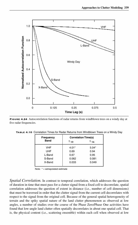
Approaches to Clutter Modeling 339

Spatial Correlation. In contrast to temporal correlation, which addresses the questionof duration in time that must pass for a clutter signal from a fixed cell to decorrelate, spatialcorrelation addresses the question of extent in distance (i.e., number of cell dimensions)that must be traversed in order that the clutter signal from the current cell decorrelates withrespect to the signal from the original cell. Because of the general spatial heterogeneity ofterrain and the spiky spatial nature of the land clutter phenomenon as observed at lowangles, a number of studies over the course of the Phase Zero/Phase One activities havefound that low-angle land clutter often spatially decorrelates in about one spatial cell. Thatis, the physical content (i.e., scattering ensemble) within each cell when observed at low

Figure 4.24 Autocorrelation functions of radar returns from windblown trees on a windy day at five radar frequencies.

Table 4.10 Correlation Times for Radar Returns from Windblown Trees on a Windy Day

0 0.125 0.25 0.375 0.5

S-Band

X-Band

UHF

VHF

L-Band

Windy Day

1.0

0.8

0.6

0.4

0.2

0.0

Time Lag (s)

No

rmal

ized

Au

toco

rrel

atio

n F

un

ctio

n

FrequencyBand

Correlation Time(s)� �1/2 1/e

Note: * = extrapolated estimate

5.04*0.940.950.0810.049

4.01*0.690.670.0620.033

VHFUHF

L-BandS-BandX-Band

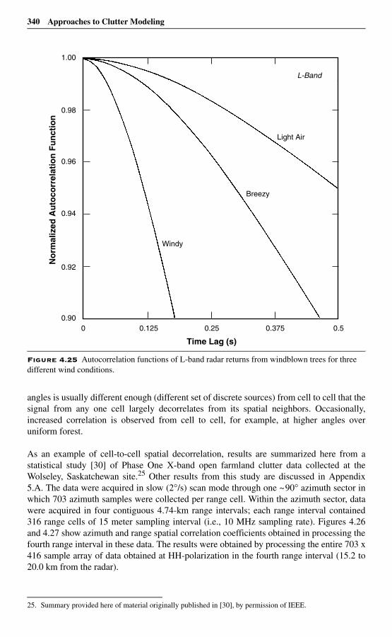
340 Approaches to Clutter Modeling

angles is usually different enough (different set of discrete sources) from cell to cell that thesignal from any one cell largely decorrelates from its spatial neighbors. Occasionally,increased correlation is observed from cell to cell, for example, at higher angles overuniform forest.

As an example of cell-to-cell spatial decorrelation, results are summarized here from astatistical study [30] of Phase One X-band open farmland clutter data collected at theWolseley, Saskatchewan site.25 Other results from this study are discussed in Appendix5.A. The data were acquired in slow (2°/s) scan mode through one ~90° azimuth sector inwhich 703 azimuth samples were collected per range cell. Within the azimuth sector, datawere acquired in four contiguous 4.74-km range intervals; each range interval contained316 range cells of 15 meter sampling interval (i.e., 10 MHz sampling rate). Figures 4.26and 4.27 show azimuth and range spatial correlation coefficients obtained in processing thefourth range interval in these data. The results were obtained by processing the entire 703 x416 sample array of data obtained at HH-polarization in the fourth range interval (15.2 to20.0 km from the radar).

Figure 4.25 Autocorrelation functions of L-band radar returns from windblown trees for three different wind conditions.

25. Summary provided here of material originally published in [30], by permission of IEEE.

0 0.125 0.25 0.375 0.5

L-Band

Windy

Breezy

Light Air

1.00

0.98

0.96

0.94

0.92

0.90

Time Lag (s)

No

rmal

ized

Au

toco

rrel

atio

n F

un

ctio

n

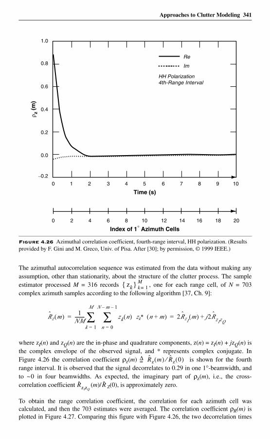
Approaches to Clutter Modeling 341

The azimuthal autocorrelation sequence was estimated from the data without making anyassumption, other than stationarity, about the structure of the clutter process. The sampleestimator processed M = 316 records , one for each range cell, of N = 703complex azimuth samples according to the following algorithm [37, Ch. 9]:

where zI(n) and zQ(n) are the in-phase and quadrature components, z(n) = zI(n) + jzQ(n) isthe complex envelope of the observed signal, and * represents complex conjugate. InFigure 4.26 the correlation coefficient ρz(m) is shown for the fourthrange interval. It is observed that the signal decorrelates to 0.29 in one 1°-beamwidth, andto ~0 in four beamwidths. As expected, the imaginary part of ρz(m), i.e., the cross-correlation coefficient (m)/ Z(0), is approximately zero.

To obtain the range correlation coefficient, the correlation for each azimuth cell wascalculated, and then the 703 estimates were averaged. The correlation coefficient ρR(m) isplotted in Figure 4.27. Comparing this figure with Figure 4.26, the two decorrelation times

Figure 4.26 Azimuthal correlation coefficient, fourth-range interval, HH polarization. (Results provided by F. Gini and M. Greco, Univ. of Pisa. After [30]; by permission, © 1999 IEEE.)

0 1

1.0

0.8

0.6

0.4

0.2

0.0

2 3 4 5 6 7 8

HH Polarization4th-Range Interval

9 10

Time (s)

ρ z (m

)

0 2 4 6 8 10 12 14 16 18 20

Re

Im

Index of 1° Azimuth Cells

–0.2

zk{ } k 1=M

zk*R̂z m( ) 1

NM--------- zk n( )

n 0=

N m– 1–

∑k 1=

M

∑= n m+( ) 2R̂zIm( ) j2R̂zIzQ

+=

∆= R̂z m( ) R̂z⁄ 0( )

R̂zIzQR̂

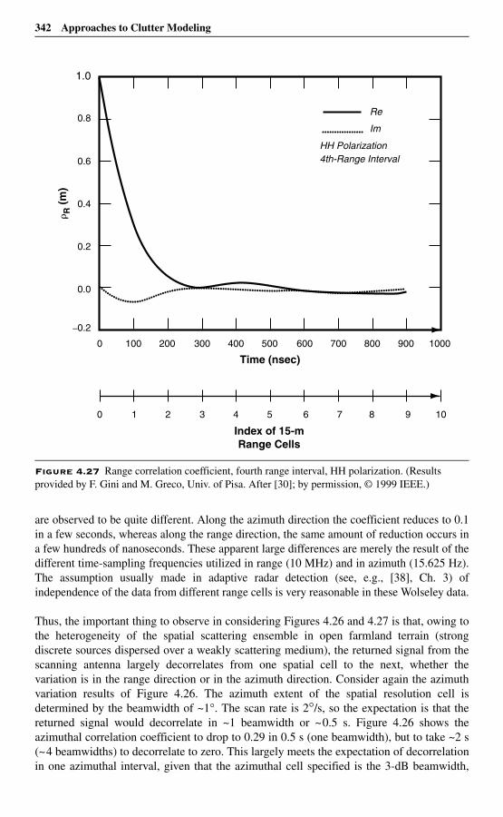
342 Approaches to Clutter Modeling

are observed to be quite different. Along the azimuth direction the coefficient reduces to 0.1in a few seconds, whereas along the range direction, the same amount of reduction occurs ina few hundreds of nanoseconds. These apparent large differences are merely the result of thedifferent time-sampling frequencies utilized in range (10 MHz) and in azimuth (15.625 Hz).The assumption usually made in adaptive radar detection (see, e.g., [38], Ch. 3) ofindependence of the data from different range cells is very reasonable in these Wolseley data.

Thus, the important thing to observe in considering Figures 4.26 and 4.27 is that, owing tothe heterogeneity of the spatial scattering ensemble in open farmland terrain (strongdiscrete sources dispersed over a weakly scattering medium), the returned signal from thescanning antenna largely decorrelates from one spatial cell to the next, whether thevariation is in the range direction or in the azimuth direction. Consider again the azimuthvariation results of Figure 4.26. The azimuth extent of the spatial resolution cell isdetermined by the beamwidth of ~1°. The scan rate is 2°/s, so the expectation is that thereturned signal would decorrelate in ~1 beamwidth or ~0.5 s. Figure 4.26 shows theazimuthal correlation coefficient to drop to 0.29 in 0.5 s (one beamwidth), but to take ~2 s(~4 beamwidths) to decorrelate to zero. This largely meets the expectation of decorrelationin one azimuthal interval, given that the azimuthal cell specified is the 3-dB beamwidth,

Figure 4.27 Range correlation coefficient, fourth range interval, HH polarization. (Results provided by F. Gini and M. Greco, Univ. of Pisa. After [30]; by permission, © 1999 IEEE.)

0 100

1.0

0.8

0.6

0.4

0.2

0.0

200 300 400 500 600 700 800

HH Polarization4th-Range Interval

900 1000

� R (

m)

0 1 2 3 4 5 6 7 8 9 10

Re

Im

–0.2

Index of 15-mRange Cells

Time (nsec)

Approaches to Clutter Modeling 343

with resultant beam overlap between 1° cells. The azimuth sampling rate used in dataacquisition was 15.625 samples (pulses) per second. That is, in azimuth, the sampling time(0.064 s, is much less than the cell size (~0.5 s).

Now consider again the range variation results shown in Figure 4.27. The range extent ofthe spatial resolution cell is determined by the 3-dB pulse length which is specified to be100 ns. This is matched to the range sampling rate of 10 MHz (i.e., in range, the samplinginterval equals the cell size). Therefore, the expectation is that, in range, the returned signalwould largely decorrelate, sample-to-sample, in ~100 ns. Figure 4.27 shows the rangecorrelation coefficient to drop to 0.3 in 100 ns (one pulse length), but it takes 300 ns (3pulse lengths) to decorrelate to zero. Thus the range results of Figure 4.27 very closelymatch the azimuthal results of Figure 4.26 in terms of equivalent cell-to-cell decorrelationin azimuth and range.

Note that although the azimuthal decorrelation in Figure 4.26 is caused by the antennapattern, the decorrelation data cannot be simply predicted from the pattern. Perhaps itwould be useful to state a simple example as follows: if the pattern were hypotheticallypurely rectangular (i.e., a simple step function of width φ), and if the clutter were simplyone large point scatterer, then the azimuthal correlation coefficient would be triangular ofbase width 2φ (i.e., would fall to 0.5 in one cell and to zero in two cells). By contrast, themeasured data in Figure 4.26 falls to 0.29 in one cell and to zero in four cells.

4.7 SummaryChapter 4 describes a number of approaches for modeling low-angle land clutter insurface-sited radar. As a physical phenomenon, the most salient attribute of low-angleclutter is variability. Two important ways in which this variability is evidenced arepatchiness in spatial occurrence and extremely wide cell-to-cell statistical fluctuation inclutter strength (i.e., spikiness) within patches. A site-specific approach to cluttermodeling is described based on the use of digitized terrain elevation data (DTED) at eachsite, which captures both of these basic attributes—patchiness, via deterministiccomputation of geometric terrain visibility from the radar site; and spikiness, viarealizations from statistical distributions in which the spread depends on the depressionangle to the backscattering terrain point as computed from the DTED.

An interim site-specific clutter model is provided as a table of Weibull coefficients inwhich the mean value of the distribution of clutter strengths varies with radar frequency,the shape parameter of the distribution varies with radar spatial resolution, and both meanstrength and shape parameter vary with depression angle and terrain type. This site-specific approach to clutter modeling in surface radar is highly realistic. Besides capturingthe fundamental patchiness and spikiness of low-angle clutter, this approach: (a) ensuresthat the modeled clutter in surface-sited radar dissipates with increasing range in the sameway that clutter actually dissipates with increasing range at real sites, namely, via thedeterministic visibility function, whereby the spatial patches of occurrence of clutterbecome fewer and farther apart with increasing range until, beyond some maximum range,no more clutter patches are visible; and (b) raises clutter modeling to the level of aquantitative science in that a given clutter patch at a given site, and, more specifically, thedistribution of clutter strengths over that patch is a real and distinct physical entity that canbe measured, parameterized (e.g., by terrain type and depression angle), and modeled, thus

344 Approaches to Clutter Modeling

allowing quantitative comparison of the measured and modeled distributions and hence adirect means for clutter model validation.

Dominant sources of low-angle clutter appear to be of a point-like or spatially discretenature, in that they occur in spatially isolated cells as opposed to being of a spatiallyextended nature. The basic site-specific approach to clutter modeling does not distinguishbetween whether clutter returns emanate from discrete or extended sources. A refinementto the basic site-specific clutter model is described involving a more computationallyintensive approach that separates the modeling of dominant, locally strong clutter cells(called the discrete component) from weaker surrounding clutter cells (called thebackground component). Little correlation was found to exist between clutter cells that arelocally stronger than their neighbors, and actual physical discrete objects on the terrain thatcould be identified as the sources of the strong clutter. Furthermore, it is not possible todetermine in the measurement data whether a given, locally strong clutter return actuallyemanates from a definable, physical point object of specifiable RCS, or from a physicallyextended σ° clutter medium that by chance phasor reinforcement happens to produce astrong clutter return.

Therefore, the separate modeling of locally strong clutter cells under this approach neededto be carried out, not as a deterministic RCS overlay, but as a second statistical σ° processin which, with a specified probability of occurrence, a given cell might have a “discrete”component added vectorally to its “background” component. That is, under this approachan investigator is not provided with a single value of σ° for a given terrain type andillumination angle, but is provided with two values of σ°, one for “discrete” clutter and onefor “background” clutter. The total clutter return is comprised of two components requiringtwo random draws, compared to modeling the total return as a single component obtainedfrom one random draw.

In the separation of locally strong clutter cells from the weaker surrounding cells, theweaker clutter was found to be dependent at the resolution cell level on terrain slope andgrazing angle, thus allowing the effect of landform on the weaker clutter to be provided atthe cell level via computation of grazing angle using DTED rather than through macropatchclassification of terrain relief; the locally strong (i.e., dominant) clutter, like the total clutterin the interim model, did not show correlation with grazing angle at the cell level. Anotherrefinement to the basic site-specific clutter model obtainable with more intensivecomputation is the softening or blurring of shadow boundaries, as determinedgeometrically from DTED, whereby clutter is allowed to rapidly diminish into shadowedregions with increasing depth of shadow rather than abruptly terminating right at theshadow boundary.

These site-specific approaches to clutter modeling allow the limiting effects of clutter onradar system performance at any given site to be determined to a high degree of exactitude,thereby meeting much in the way of design- and analysis-related need for quantificationand prediction of radar performance in ground clutter. In today’s highly evolved and rapidlyexpanding era of high performance computer capability, the fact that a site-specificapproach to clutter modeling is computer-dependent, requiring extensive computationbased on accurate DTED for the sites in question, is no longer very restrictive, whetherconcern is with individual sites or complexes of sites. The nature of ground clutter is that itcan affect radar performance very differently from site to site, as a consequence of the

Approaches to Clutter Modeling 345

extreme variations in surrounding terrain that can occur from one site to another, and aquantitative approach to the accurate assessment of the effects of clutter needs to reflectthis specificity.

Nevertheless, the fact remains that the site-specific approach to modeling clutter providesanswers one site at a time. For radar system design/analysis that requires more generalinformation of the impact of ground clutter on system performance, the rigorous way underthe site-specific approach is to first compute performance across a set of sites as specifiedby the particular design or analysis under consideration, and then to generalize (e.g.,medianize) performance depending on how site-to-site performance varies across the set.Note that this approach to generality a posteriori averages the performance measuresobtained from a number of realistic site-specific clutter computations; it does not attempt toa priori average the clutter first (a non-verifiable undertaking) followed by a one-timeassessment of performance.

As a conceptual alternative to accepting the computational burden required in such arigorous approach to generality, the idea of a clutter model that retains the importantelement of spatial patchiness but realizes it by means of a generic stochastic process inwhich patch extents, separations, and obliquities are statistically representative of generaltypes of terrain rather than specific sites is intuitively attractive. This idea, involvingimplementation of generalized stochastic patchiness, although beyond the range of subjectmatter covered in this book, was explored at some length in coordinated studies involvingthe Lincoln Laboratory clutter data carried out by other investigative agencies ([3] is anearly citation from extended research undertaken to develop this idea). However, thespecificity of terrain feature at the scale at which terrain feature affects low-angle terrainvisibility and clutter patchiness makes it difficult to capture such effects statistically. Unlikethe ocean, the terrain at most sites of any significant relief is not very statistical in the senseof generally repeated patterns, but is dominated by a relatively few discrete singularmacrofeatures (e.g., a mountain range, a ridge of hills, a river valley, a coastal shoreline).As a result, the parameters affecting the patchiness provided by a general stochastic modelcould not be related to simple quantifiable measures (e.g., surface relief; correlationdistance) associated with generalized terrain types; but rather required that the parametersgoverning patchiness be acquired by an initialization or conditioning cycle of processing inDTED over a large-scale region encompassing the site of interest.

Such generalized approaches to stochastic patchiness were reasonably successful for terrainof relatively low or moderate relief; high-relief terrain is too specific for a stochasticapproach to be appropriate. Since a stochastically patchy non-site-specific clutter modelrequires initialization using DTED from the terrain region of interest, the sought foradvantages of such a model in providing non-site-specific stochastic realizations ofpatchiness are somewhat diminished compared with more straightforwardly obtained site-specific realizations of patchiness. For such reasons, the initially attractive and deceptivelysimple notion of a generic non-site-specific clutter model invested with realistic stochasticpatchiness becomes more difficult to successfully implement in actual practice than mightbe presupposed, although a remaining advantage of the stochastically patchy approach isthat it can lead to generic analytic formulations of such system performance measures as,for example, signal-to-clutter ratio vs range for the terrain type under consideration.

346 Approaches to Clutter Modeling

A spatially patchy clutter model, whether site-specific or non-site-specific, captures theimportant element of disconnectedness in spatial occurrence of low-angle terrain visibilitythat leads to a high degree of fidelity in the representation of ground clutter in surface radar.Such a high degree of fidelity is not always required, however, in the representation ofground clutter by radar system engineers. As a first indication of the effects of groundclutter, the radar system engineer may not be interested in the full-blown system effects ofpatchiness, but may require only a single value of constant σ° indicating how strong theclutter is at a given site for use in the radar range equation to estimate signal-to-clutterratios against particular targets; and in addition may require only a single value of cut-offrange to indicate the maximum extent in range to which the constant σ° applies and beyondwhich the radar is clutter-free.

From this point of view, the modeling of patchiness in low-angle terrain visibility may beregarded as a higher order (although important) effect in low-angle clutter phenomenologycompared with modeling the strength of the clutter (assuming that the ground is visible),and for a beginning all that is required of this higher-order effect is a global estimate of themaximum extent of the patchy terrain visibility in range. Furthermore, this point of viewdisregards the fact that low-angle σ° occurs as a statistical phenomenon with wide cell-to-cell variations over a local region, but instead focuses on a single measure of strength suchas the mean level; it also disregards the fact that σ° varies with depression angle sincedepression angle varies most significantly only within the first few kilometers of rangefrom the radar, and usually diminishes to very near grazing incidence (e.g., 0.1° or 0.2°)over the much greater extents of clutter spatial occupancy that occur at much longer ranges.

To meet these kinds of less demanding requirements in a clutter model, Chapter 4 alsoprovides a simple, non-patchy, non-site-specific clutter model that specifies mean clutterstrength depending only on general terrain type (e.g., rural/low-relief, rural/high-relief, urban) and clutter cut-off range Rc depending only on effective radar height (e.g.,low, intermediate, high). Since low-angle clutter is so variable both in strength and extent,these two parameters and Rc are provided not only as baseline central values, but alsoas worst-case values indicative of severe or heavy clutter situations, and as best-case valuesindicative of benign or light clutter situations.

A very large step in simplification occurs between the extremes of clutter models (viz., thefull-blown site-specific statistical model vs the simple non-site-specific constant-σ° model)described in Chapter 4. Many of the difficulties that face efforts to bring realism toempirical clutter models at intermediate levels of fidelity between these two extremes areexplored in ancillary discussions of the measured clutter data both in the body of Chapter 4and its appendices. These ancillary discussions include considerations of (a) the inherenteffects on terrain visibility and clutter strength of radar height and radar range; (b) theproper way to deal with unavoidable noise-level samples in clutter measurements and theimportant consequent effect on clutter statistics of rapidly decreasing radar sensitivity toclutter with increasing range; and (c) the wide range of variability involved in generalclutter amplitude statistics and the attendant difficulty in specifying any particular σ° levelfor a constant-σ° clutter model.

Discussions are also provided concerning the relationship between terrain visibility andclutter occurrence and concerning discrete vs distributed clutter and the appropriateparameter by which to characterize low-angle clutter. All these discussions serve to more

σ °w

σ °w

Approaches to Clutter Modeling 347

fully describe the complex, multifaceted nature of low-angle clutter from differentperspectives and to bring home the value of the site-specific approach to clutter modeling inthat it automatically and accurately incorporates all the complicating factors that are difficultfor more general modeling approaches to capture. Although the main subject of Chapter 4 isthe consideration of various approaches to modeling the spatial amplitude statistics of low-angle ground clutter, brief consideration is also given to aspects of the phenomenonassociated with its temporal variability and its spectral and correlative properties.

References1. M. Sekine and Y. Mao, Weibull Radar Clutter, London, U. K.: Peter Peregrinus Ltd.

and IEE, 1990.

2. R. R. Boothe, “The Weibull Distribution Applied to the Ground Clutter BackscatterCoefficient,” U. S. Army Missile Command Rept. No. RE-TR-69-15, RedstoneArsenal, AL, June 1969; DTIC AD-691109.

3. S. P. Tonkin and M. A. Wood, “Stochastic model of terrain effects upon theperformance of land-based radars,” AGARD Conference Proceedings on Target andClutter Scattering and Their Effects on Military Radar Performance, AGARD-CP-501, (1991).

4. M. P. Warden and E. J. Dodsworth, “A Review of Clutter, 1974,” Royal RadarEstablishment Technical Note No. 783, Malvern, U.K., September 1974; DTIC ADA014421.

5. W. J. McEvoy, “Discrete Clutter Measurements Program: Operations in theMetropolitan Boston Area,” MITRE Corporation; Air Force Systems Command,Electronic Systems Division, Deputy for AWACS, Report ESD-TR-72-131, AD 742298, March 1972.

6. W. J. McEvoy, “Discrete Clutter Measurements Program: Operations in WesternMassachusetts,” MITRE Corporation; Air Force Systems Command, ElectronicSystems Division, Deputy for AWACS, Report ESD-TR-72-132, AD 742 297,March 1972.

7. D. C. Schleher, MTI and Pulsed Doppler Radar, Norwood, MA: Artech House,1991, p. 226.

8. S. Kazel, J. Patten, J. Dabkowski, J. Pipkin, and A. Brindley, “Extensions to the ORTClutter Model,” IIT Research Institute, Chicago, June 1971.

9. H. R. Ward, “A model environment for search radar evaluation,” IEEE EASCON Rec,pp. 164-171, 1971.

10. C. J. Rigden, “High Resolution Land Clutter Characteristics,” Admiralty SurfaceWeapons Establishment Technical Report TR-73-6, Portsmouth, U.K., January 1973;DTIC AD-768412.

11. D. C. Schleher, op. cit., p. 174.

12. C. W. Helstrom, Elements of Signal Detection and Estimation, Englewood Cliffs, NJ:Prentice-Hall, 1995.

348 Approaches to Clutter Modeling

13. T. Linell, “An experimental investigation of the amplitude distribution of radarterrain return,” 6th Conf. Swedish Natl. Comm. Sci. Radio, Research Institute ofNational Defence, Stockholm, March 1963.

14. F. E. Nathanson and J. P. Reilly, “Clutter statistics that affect radar performanceanalysis,” EASCON Proc. (supplement to IEEE Trans.), vol. AES-3, no. 6, pp. 386-398, November 1967.

15. J. K. Jao, “Amplitude distribution of composite terrain radar clutter and the K-distribution,” IEEE Transactions on Antennas and Propagation, AP-32 (Oct. 1984),1049-1062.

16. J. B. Billingsley and J. F. Larrabee, “Multifrequency Measurements of Radar GroundClutter at 42 Sites,” Lexington, MA: MIT Lincoln Laboratory, Technical Rep. 916,Volumes 1, 2, 3; 15 November 1991; DTIC AD-A246710.

17. K. Rajalakshmi Menon, N. Balakrishnan, M. Janakiraman, and K. Ramchand,“Characterization of fluctuating statistics of radar clutter for Indian terrain,” IEEETransactions on Geoscience and Remote Sensing. vol. 33. no. 2 (March 1995), 317-323.

18. V. Anastassopoulos and G. A. Lampropoulos, “High resolution radar clutterclassification,” in Proceedings of IEEE International RADAR Conference,Washington, DC, May 1995, 662-667.

19. K. S. Chen and A. K. Fung, “Frequency dependence of backscattered signals fromforest components,” IEE Proceedings, Pt. F, 142, 6 (December 1995), pp. 310-315.

20. E. J. Barlow, “Doppler Radar”, Proc. IRE, 37, 4 (1949).

21. J. L. Lawson and G. E. Uhlenbeck (eds), Threshold Signals, Vol. 24 in the MITRadiation Laboratory Series, New York: McGraw-Hill (1950). Reprinted, DoverPublications (1965).

22. H. Goldstein, “The Fluctuations of Clutter Echoes,” pp. 550-587, in D. E. Kerr (ed.),Propagation of Short Radio Waves, Vol. 13 in the MIT Radiation Laboratory Series,New York: McGraw-Hill (1951). Reprinted, Dover Publications (1965).

23. J. B. Billingsley, A. Farina, F. Gini, M. V. Greco, and P. Lombardo, “Impact ofexperimentally measured Doppler spectrum of ground clutter on MTI and STAP,” inProceedings of 1997 International Radar Conference, Edinburgh, UK, October 14-16, 1997, 290-294.

24. A. Farina, F. Gini, M. V. Greco, and P. Lee, “Improvement factor for real sea-clutterDoppler frequency spectra,” IEE Proceedings, Pt. F, 143, 5 (October 1996), 341-344.

25. S. Watts, C. J. Baker, and K. D. Ward, “Maritime surveillance radar Part 2: Detectionperformance prediction in sea clutter,” IEE Proceedings, Pt. F, 137, 2 (April 1990),63-72.

26. J. B. Billingsley and J. F. Larrabee, “Measured Spectral Extent of L- and X-BandRadar Reflections from Windblown Trees,” Lexington, MA: MIT LincolnLaboratory, Project Rep. CMT-57, 6 February 1987; DTIC AD-A179942.

27. H. C. Chan, “Radar ground clutter measurements and models, part 2: Spectralcharacteristics and temporal statistics,” AGARD Conference Proceedings on Target

Approaches to Clutter Modeling 349

and Clutter Scattering and Their Effects on Military Radar Performance, AGARD-CP-501 (1991).

28. G. C. Sarno, “A model of coherent radar land backscatter,” AGARD ConferenceProceedings on Target and Clutter Scattering and Their Effects on Military RadarPerformance, AGARD-CP-501 (1991).

29. J. B. Billingsley, “Exponential Decay in Windblown Radar Ground Clutter DopplerSpectra: Multifrequency Measurements and Model,” Lexington, MA: MIT LincolnLaboratory, Technical Report 997, 29 July 1996; DTIC AD-A312399.

30. J. B. Billingsley, A. Farina, F. Gini, M. V. Greco, and L.Verrazzani, “Statisticalanalyses of measured radar ground clutter data,” IEEE Trans. AES, vol. 35, no. 2(April 1999).

31. P. Lombardo, and J. B. Billingsley, “A new model for the Doppler spectrum ofwindblown radar ground clutter,” in Proceedings of IEEE 1999 Radar Conference,Boston, MA, 20-22 April 1999.

32. D. P. Meyer and H. A. Mayer, Radar Target Detection—Handbook of Theory andPractice, San Diego, CA: Academic Press, 1973, pp. 66, 67.

33. L. R. Rabiner and B. Gold, Theory and Application of Digital Signal Processing,Prentice-Hall, Inc., Englewood Cliffs, NJ, 1975.

34. F. J. Harris, “On the use of windows for harmonic analysis with the discrete Fouriertransform,” Proc. IEEE, vol. 66, no. 1, pp. 51-83, January 1978.

35. V. A. Andrianov, N. A. Armand, and I. N. Kibardina, “Scattering of radio waves byan underlying surface covered with vegetation,” Radio Eng. and Electron. Physics(USSR), vol. 21, no. 9, September 1976.

36. C. M. Rader, “An improved algorithm for high-speed autocorrelation withapplications to spectral estimation,” IEEE Trans. Audio Electrocoustic., vol. AU-18,pp. 439-441, Dec. 1970.

37. S. M. Kay, Fundamentals of Statistical Signal Processing: Estimation Theory,Englewood Cliffs, NJ: Prentice-Hall, 1993.

38. S. Haykin and A. Steinhardt, Adaptive Radar Detection and Estimation, New York:Wiley, 1992.

5MULTIFREQUENCY LAND CLUTTER

MODELING INFORMATION

5.1 IntroductionChapter 5 provides land clutter modeling information for surface-sited radar based oncomprehensive reduction of extensive multifrequency land clutter measurement data from42 different sites. The survey clutter measurements upon which this information is basedare described in Chapter 3 (see also [1]). The clutter modeling information that follows isprovided for general terrain and for eight specific terrain types. For each terrain type, themodeling information is further partitioned by the relief of the terrain and by thedepression angle below the horizontal from the radar to the backscattering terrain point.

For each terrain type/relief/depression angle combination of parameters, the modelinginformation provided specifies the probability distribution encompassing the spatial cell-to-cell variability of clutter amplitude statistics applicable to that combination ofparameters. Probability distributions are specified in terms of Weibull statistics. For eachterrain type/relief/depression angle combination, Weibull mean clutter strength isprovided as a function of radar frequency, VHF to X-band; and Weibull shape parameteraw is provided as a function of radar spatial resolution, 103 m2 to 106 m2. The number ofclutter coefficients applicable to low-angle land clutter specified in Chapter 5 is 864.These coefficients are provided within a parametric structure that allows practicalapplication of them to surface radars sited in various terrains and situations.

Most of the clutter coefficients provided are relatively general, each usually being basedon numerous measurements. The number of measurements applicable to each value of

is also provided. In the past, authoritative reviews of the subject [2–5] have agreedon the difficulty of characterizing low-angle land clutter with basic questions of radarfrequency dependence, the role of illumination angle, and effects of varying terrain typeremaining unanswered. The definitive body of new information presented in Chapter 5now provides a condensed and unified codification of low-angle land clutter’sfundamental attributes.

In what follows, Section 5.1.1 reviews the Phase One survey database, the reduction ofthese data into patch-specific histograms of clutter strength, and the fundamentalparametric effects that emerge in the trend analyses of these histograms. Section 5.2describes how clutter modeling information in terms of Weibull statistics is derived throughthe combination of many patch measurements. Section 5.3 presents clutter modelinginformation for general rural terrain, irrespective of land cover. Section 5.4 presents cluttermodeling information for eight specific terrain types. Section 5.5 briefly discusses and

σ °w

σ °w

σ °w

408 Multifrequency Land Clutter Modeling Information

provides an example of plan-position indicator (PPI) clutter map simulation using themodeling information of Chapter 5. Section 5.6 is a summary. Appendix 5.A presentsadditional information on Weibull statistics and compares them with statistics fromlognormal and K-distributions.

5.1.1 Review

5.1.1.1 Clutter MeasurementsThe results of Chapter 5 are based on Phase One five-frequency land clutter measurementsat 42 different sites as described in Chapter 3. At each Phase One site, all of the discernibleland clutter within the field-of-view was measured at each of five frequencies, VHF, UHF,L-, S-, and X-bands, and at both vertical and horizontal polarization and at low and highrange resolution. These raw Phase One data were calibrated, pulse-by-pulse and cell-by-cell, into absolute units of clutter strength. The resultant large 475-Gbyte five-frequencyland clutter measurement database comprises a unique resource that is planned to bemaintained indefinitely at Lincoln Laboratory. These data were provided to governmentauthorities in Canada and the United Kingdom, and coordinated analyses took place inthese countries as well as in the United States [6–9]. The results of Chapter 5 are based onthe spatially comprehensive 360° survey data from all 42 Phase One sites. Previous PhaseOne results discussed in Chapters 3 and 4 were based on the relatively narrow (e.g., 20°)azimuth sector of repeated measurement concentration at each site called the repeat sector.Clutter experiments acquired in survey mode, as opposed to repeat sector mode, arefurther described in Chapter 3, Section 3.2.2.

5.1.1.1.1 Data Reduction

Each raw in-phase (I) and quadrature (Q) sample pair of Phase One measured clutter datais reduced to a clutter strength number. As defined earlier in this book, clutter strength isgiven by σ °F4, where σ ° is the intrinsic backscattering coefficient and F is the patternpropagation factor. As previously discussed, the pattern propagation factor includes allterrain effects in low-angle land clutter caused by multipath reflections and diffractionfrom the terrain. Using available digitized terrain elevation data, it is not generallypossible to deterministically compute F at clutter source heights sufficiently accurately toallow cell-by-cell separation of intrinsic σ ° in measured clutter data (e.g., see Chapter 1,Section 1.5.4; Chapter 3, Appendix 3.B). All of the coefficients of clutter strengthtabulated as modeling information in Chapter 5 include propagation effects. Allcomputations involving σ °F4 are performed in units of m2/m2. For convenience, thetabulated clutter coefficients have been subsequently converted to decibels with respect to1 m2/m2. The specific computations involved in data reduction are defined morecompletely in Chapters 2 and 3.

5.1.1.1.2 Stored Clutter Histograms

Within the PPI spatial map of measured clutter strength at each site, terrain macroregionswere selected largely within line-of-sight illumination in which a relatively highpercentage of resolution cells contain discernible clutter above the radar noise level. Theseterrain macroregions are referred to as terrain patches or clutter patches. Typically, clutterpatches are several kilometers on a side (median size = 12.6 km2; see Appendix 2.B).Many examples of clutter patches and histograms of clutter strength measured from clutterpatches are shown in this book, including several to follow in Chapter 5. By registeringmeasured clutter maps with air photos and topographic maps, landform and land coverdescriptive information of the terrain within the patch was provided.

Multifrequency Land Clutter Modeling Information 409

The landform and land cover classification systems utilized in this process are described inChapter 2, Section 2.2.3. For each clutter patch, the distribution or histogram of clutterstrengths occurring within the patch was formed, based upon all of the cells within the patch,including those at radar noise level. This histogram was formed at each of the 20 parametercombinations nominally available within the Phase One radar parameter matrix (fivefrequencies, two polarizations, two range resolutions; see Appendix 3.A, Table 3.A.2).Various statistical attributes (e.g., mean, median, variance, etc.) of each histogram werecomputed. The formulas used in these computations are provided in Appendices 2.B and 3.C.

Each histogram together with its statistical attributes and the applicable terrain descriptorsof the patch and the radar parameters was then stored in a computer file. Predictive cluttermodeling information was developed by establishing general correlative propertiesbetween the stored distributions of measured clutter strength and the corresponding terraindescriptions and relevant radar parameters. The results of Chapter 5 are based on 59,804stored histograms of measured clutter strength from 3,361 clutter patches at the 42 PhaseOne sites.

5.1.1.1.3 Pure and Mixed Terrain

Classification of the terrain within each of the 3,361 clutter patches in terms of landform(i.e., the relief or roughness of the terrain) and land cover (e.g., urban, forest, agricultural,etc.) occurred at two levels, primary and secondary (see Sections 2.2.3 and 3.2.3 fordetails). As a result of terrain classification, the results of Chapter 5 are partitioned intotwo groups, those applicable to pure terrain and those applicable to mixed terrain. Pureterrain is terrain that requires primary classification only. Mixed terrain requires secondaryas well as primary classification. Of the 3,361 clutter patches, 1,733 (i.e., 52%) are pureand 1,628 (i.e., 48%) are mixed. For pure terrain, clutter modeling results are provided inSection 5.4 for eight specific terrain types; namely, urban, agricultural, forest, shrubland,grassland, wetland, desert, and mountain categories. These specific terrain types areusually characterized principally by land cover, although mountain terrain is characterizedprincipally by landform. For mixed terrain, general results are provided in Section 5.3.

Most terrain types are further partitioned by relief, usually in terms of high relief (i.e.,with terrain slopes > 2°) and low relief (i.e., with terrain slopes < 2°). Results for pureterrain are suitable for modeling at cell level or in very homogeneous terrain. Results forpure terrain are also useful for setting approximate worst-case/best-case bounds on theseverity of land clutter interference. Results for mixed terrain apply more generally tolarge extents of composite landscape. The results in Section 5.3 for general mixed ruralterrain are among the more important results of the Phase One clutter measurementsprogram; these results show how systematic variations in terrain relief and depressionangle cause corresponding variations in clutter strength in all five frequency bands forgenerally occurring composite terrain.

5.1.1.1.4 Clutter Patch Selection at Magrath

Figure 5.126 illustrates clutter patch selection at the Phase One measurement site ofMagrath, Alberta. The figure shows two Phase One X-band PPI clutter maps in both ofwhich clutter is shown dark gray—the clutter map on the left is to 20-km maximum range,that to the right is to 50-km maximum range. In both clutter maps, the repeat sector clutterpatch is shown as a narrow solid black sector to the southeast. Repeat sector clutter

26. All Chapter 5 figures occur consecutively in the figures-only, color section beginning on page 447.

410 Multifrequency Land Clutter Modeling Information

measurements, involving one patch per site at each of 42 different sites, are the basis of thePhase One results provided in Chapters 3 and 4.

Also in both clutter maps, all the survey patches selected at Magrath are shown outlinedand shaded to appear light gray. It is evident that the survey patches in total are much morespatially comprehensive in terms of covering almost all of the measured clutter than therepeat sector. As a result, the clutter modeling information of Chapter 5, based on surveymeasurements at all sites, is of increased statistical certainty and of increased predictionaccuracy, both because these survey results are based on many more samples per terrainclass and in addition because they are based on more terrain classes.

5.1.1.1.5 Noise Corruption

It was indicated above that, in forming histograms and cumulative distributions of clutterstrength σ °F4 over clutter patches, all of the cells and samples that were measured fromthe patch, including those at radar noise level, need to be included. It is possible, informing such histograms and distributions, to include only those samples for which thereturned signal strength is greater than radar noise level, and to delete the noise-levelsamples. Such histograms and distributions have been referred to as “shadowless”previously in this book (e.g., see Section 1.4.7 and Appendices 2.B, 3.C, and 4.C forrelated discussions). Shadowless statistics are obviously dependent upon radar sensitivityand are thus conditional (not absolute) measures of reflectivity. Use of shadowless clutterstatistics can lead to subsequent misinterpretation in analysis and significantmisrepresentation of radar system performance.

Thus, in forming the cumulative distribution for a given clutter patch, the noise-levelsamples are retained and the cumulative is plotted two ways: (1) as an upper bound inwhich the samples at noise level retain their noise power values, and (2) as a lower bound inwhich the samples at noise level are assigned zero (or a very low value of) power. Theseupper bound/lower bound cumulative pairs deviate from each other only over the low-endnoise-corrupted interval of the distribution (where the true cumulative must lie betweenthem); they merge to form the single true cumulative at σ°F4 levels above the highest noisecorruption. By true cumulative is meant that which would be measured by a hypotheticalradar of infinite sensitivity (or at least sensitivity high enough so that all clutter samplesreturned from the clutter patch are well above radar noise level). In contrast, the shadowlesscumulative can lie significantly apart from the true cumulative over its compete range (seeAppendix 4.C).

Similarly, in the computation of the moments of distributions that include noise samples,the moments are computed two ways: (1) as an upper bound in which the samples at noiselevel retain their noise power values, and (2) as a lower bound in which the samples at noiselevel are assigned zero power. Upper and lower bounds to moments of noise-corruptedclutter distributions are usually within small fractions of a decibel of each other, even whenthe amount of noise corruption is high; such tight bounds are the result of the extremeskewness of the distributions such that the moments are dominated by the high-end tails. Ofcourse, the true value of the moment must lie between the upper and lower bounds. Incontrast, moments of shadowless distributions are dependent on radar sensitivity (i.e., theamount of noise that was deleted) and can be significantly different from the true value.Separation of upper and lower bound values of moments by large amounts indicates ameasurement too corrupted by noise to provide useful information.

Multifrequency Land Clutter Modeling Information 411

The clutter modeling results provided in Chapter 5 are based upon tight upper-bound valuesof moments of noise-corrupted low-angle clutter distributions and are thus absolutemeasures independent of radar sensitivity. The correct methodology (as discussed above)for the proper treatment of radar noise and shadowing in low-angle clutter is elaborated inmore detail elsewhere (see Section 1.4.7 and Appendices 2.B, 3.C, and 4.C).

5.1.1.1.6 Two Clutter Patch Histograms

The terrain within general rural clutter patches often consists of mixtures of various open(e.g., cropland, rangeland) and tree-covered components. Figures 5.2 and 5.3 showexamples of measured clutter histograms and cumulative distributions from two suchmixed rural patches. These two examples were selected from the 30,246 such histogramscomprising the Phase One general mixed rural clutter modeling database.

Figure 5.2 shows a UHF histogram measured from patch 34/2 at Wachusett Mountain,Massachusetts. Patch WM 34/2 was primarily hilly mixed-forest with secondaryoccurrences of cropland and lakes, and was observed at 1° depression angle. It wassituated beginning at 11.9 km from the radar and extended 11.7 km in range and 35.6° inazimuth. In the histogram of Figure 5.2, 4.1% of the samples are at radar noise level (cellsat noise level are indicated as black in the histogram). Figure 5.3 shows an X-bandhistogram measured from patch 7/1 at Spruce Home, Saskatchewan. Patch SH 7/1 wasprimarily level cropland with secondary occurrences of trees at 10% incidence ofoccurrence and was observed at a depression angle of 0.6°. It was situated beginning2.2 km from the radar and extended 4.8 km in range and 33.6° in azimuth. In thehistogram of Figure 5.3, 11.6% of the samples are at radar noise level. The histograms ofFigures 5.2 and 5.3 were both measured using 150-m pulse length and horizontalpolarization.

The WM 34/2 and SH 7/1 clutter histograms of Figures 5.2 and 5.3 typify the many suchmeasurements in the Phase One database in the extremely wide range of values of clutterstrength σ°F4 that each exhibits. The WM 34/2 histogram of Figure 5.2 covers over sixorders of magnitude in σ°F4; the SH 7/1 histogram of Figure 5.3 covers over eight ordersof magnitude. In addition to showing these histograms, Figures 5.2 and 5.3 also show thecorresponding upper-bound cumulative distributions in which the percent of samples ineach histogram bin is accumulated left to right across the histogram.

The cumulative distribution is shown as a solid line and is read on the left ordinate; on theright ordinate is read the percent of samples in each histogram bin. The left ordinate is anonlinear Weibull probability scale such that theoretical Weibull cumulative distributionsplot as straight lines when, as shown, the abscissa is clutter strength in decibels (seeAppendix 2.B). Both the WM 34/2 UHF cumulative clutter distribution (Figure 5.2) and theSH 7/1 X-band distribution (Figure 5.3) are relatively linear and hence reasonably wellapproximated as Weibull distributions over much of their central extents. In this respectalso, these two distributions are representative of most of the many such measurements inthe Phase One database, which are generally (but not without occasional exception) moreWeibull-like than, for example, lognormal-like or K-distribution-like. This matter isdiscussed further in Appendix 5.A.

Also shown in Figures 5.2 and 5.3 is the slope that a theoretical Rayleigh distribution takesin such plots; by Rayleigh, it is meant that the received clutter voltage signal isx

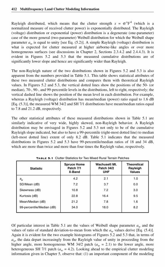
412 Multifrequency Land Clutter Modeling Information

Rayleigh distributed, which means that the clutter strength x = σ°F4 (which is anormalized measure of received clutter power) is exponentially distributed. The Rayleigh(voltage) distribution or exponential (power) distribution is a degenerate (one-parameter)case of the more general (two-parameter) Weibull distribution for which the Weibull shapeparameter aw is equal to unity [see Eq. (5.2)]. A simple Rayleigh (voltage) distribution iswhat is expected for clutter measured at higher airborne-like angles or over morehomogeneous surfaces (see discussions in Chapter 2, Sections 2.3.4.2 and 2.4.4.3). It isevident in Figures 5.2 and 5.3 that the measured cumulative distributions are ofsignificantly lower slope and hence are significantly wider than Rayleigh.

The non-Rayleigh nature of the two distributions shown in Figures 5.2 and 5.3 is alsoapparent from the numbers provided in Table 5.1. This table shows statistical attributes ofthese two measured clutter distributions and compares them with theoretical Rayleighvalues. In Figures 5.2 and 5.3, the vertical dotted lines show the positions of the 50- (ormedian), 70-, 90-, and 99-percentile levels in the distributions, left to right, respectively; thevertical dashed line shows the position of the mean level in each distribution. For example,whereas a Rayleigh (voltage) distribution has mean/median (power) ratio equal to 1.6 dB[Eq. (5.3)], the measured WM 34/2 and SH 7/1 distributions have mean/median ratios equalto 7.8 and 21.2 dB, respectively.

The other statistical attributes of these measured distributions shown in Table 5.1 aresimilarly indicative of very wide, highly skewed, non-Rayleigh behavior. A Rayleighdistribution may be envisaged in Figures 5.2 and 5.3 not only to be of the cumulativeRayleigh slope indicated, but also to have a 99-percentile (right-most dotted line) to median(left-most dotted line) extent of only 8.2 dB. Table 5.1 indicates that the measureddistributions in Figures 5.2 and 5.3 have 99-percentile/median ratios of 18 and 34 dB,which are more than twice and more than four times the Rayleigh value, respectively.

Of particular interest in Table 5.1 are the values of Weibull shape parameter aw and thevalues of ratio of standard deviation-to-mean from which the aw values derive [Eq. (5.4)].Again it is evident for the two example histograms of Figures 5.2 and 5.3 that, in terms ofaw, the data depart increasingly from the Rayleigh value of unity in proceeding from thehigher angle, more homogeneous WM 34/2 patch (aw = 2.1) to the lower angle, moreheterogeneous SH 7/1 patch (aw = 4.2). Looking ahead to the empirical clutter modelinginformation given in Chapter 5, observe that: (1) an important component of the modeling

Table 5.1 Clutter Statistics for Two Mixed Rural Terrain Patches

StatisticSpruce Home

Patch 7/1X-Band

Wachusett Mt.Patch 34/2

UHF

TheoreticalRayleighValues

aw

SD/Mean (dB)

Skewness (dB)

Kurtosis (dB)

Mean/Median (dB)

99-percentile/Median (dB)

4.2

7.2

10.8

22.8

21.2

34.0

2.1

3.7

7.2

16.4

7.8

18.0

1.0

0.0

3.0

9.5

1.6

8.2

Multifrequency Land Clutter Modeling Information 413

information is the general specification of aw as a function of resolution and depressionangle, and (2) the values of aw so specified for general low-angle clutter in ground-basedradar over large extents of composite terrain are generally far from Rayleigh and only beginto approach the Rayleigh value of unity when cell size becomes very large or as depressionangle increases to airborne-like regimes.

5.1.1.2 Parametric Effects

The following review of parametric clutter dependencies summarizes earlier discussionsin this book. As developed in Chapter 2, a fundamental parametric dependence in low-angle clutter amplitude statistics is that of depression angle as it affects microshadowingamong dominant discrete clutter sources, such that mean clutter strengths increase andcell-to-cell fluctuations decrease with increasing angle. At very low angles, clutter is to avery great extent caused by isolated discrete sources. Numerous low-reflectivity orshadowed cells occur between cells containing discrete clutter sources, even though theoverall region from which the clutter amplitude distribution is formed is under generalillumination by the radar. The combination of many shadowed or low-reflectivity weakcells together with many discrete-dominated strong cells causes extensive spread in theresultant low-angle clutter amplitude distribution.

As depression angle increases, the low reflectivity areas between discrete verticalfeatures become more strongly illuminated, resulting in less shadowing and a rapiddecrease in the spread of the distribution. As a result, measures of spread in the amplitudestatistics such as ratio of standard deviation-to-mean and mean-to-median ratio decreaserapidly with increasing angle as the shadowed and weak samples at the low end of thedistribution rise toward the stronger values that dominate the mean. However, the uppertail of the clutter distribution and mean level that is largely determined by the upper tailare still primarily caused by discrete sources and increase more slowly with increasingdepression angle. These general effects of depression angle are important at allfrequencies in the Phase One measurements.

Because of the heterogeneous process involved, wherein groups of cells providing strongreturns are often separated by cells providing weak or noise-level returns, the spatialresolution of the radar fundamentally affects the amount of spread in clutter amplitudedistributions from spatial macroregions. Increasing resolution results in less averagingwithin a cell, more cell-to-cell variability, and hence increased spread in the distributions.This general effect of resolution is also important at all frequencies in the Phase Onemeasurements.

Within the context of the above mechanisms, radar frequency does not generally play asfundamental a role as do depression angle and resolution. However, as discussed in Chapter3, two strong trends with frequency occur in particular circumstances. One of these isdirectly the result of the intrinsic backscattering coefficient σ° having an inherentfrequency-dependent characteristic. Thus, at high depression angles in forested terrain,propagation measurements show that forward reflections are minimal (i.e., F ≈1). In suchterrain, intrinsic σ° decreases strongly with increasing frequency due to the absorptioncharacteristic of forest increasing with frequency.

The other trend with frequency is the result of a general propagation effect entering clutterstrength σ°F4 through the pattern propagation factor F. At low depression angles in level

414 Multifrequency Land Clutter Modeling Information

open terrain, strong forward reflections cause multipath lobing on the free-space antennapattern. At low frequencies such as VHF, these lobes tend to be broad so that returns frommost clutter sources are received well on the underside of the first multipath lobe, andclutter strengths are much reduced. As frequency increases, the multipath lobes becomenarrower; typical clutter sources such as buildings or trees tend to extend over multiplelobes, with the result that at higher frequencies the overall multipath effect on illuminationhas less influence on the clutter strength. Thus, at low angles on level open terrain, thereexists a characteristic of strongly increasing mean clutter strength with increasingfrequency introduced through the pattern propagation factor. In inclined or rolling openterrain of increased relief, multipath is as likely to reinforce as to cancel clutter returns evenat low radar frequencies.

Polarization has little general effect on ground clutter amplitude statistics. On the average,mean ground clutter strength is often 1 or 2 dB stronger at vertical polarization than athorizontal. The reason may be associated with the preferred vertical orientation of manydiscrete clutter sources. As discussed in Chapter 3, occasional specific measurements canshow more significant variation with polarization but almost always less than 6 or 7 dB.

5.1.1.2.1 Discretes

A classical ground clutter model consists of diffuse clutter emanating from area-extensivesurfaces with a few large point-like discrete scatterers added in to account for objects likewater towers. The Phase One measurements reveal that, at the near grazing incidence ofsurface radar, over ranges of many kilometers, a more realistic construct is to imagineclutter as arising from a sea of discretes. By discretes are meant here strong, locally isolatedclutter cells separated by weak cells often at the noise level of the radar. For example, overforest, it is the cells containing projecting treetops that cause the dominant backscatter, withthe in-between shadowed areas of the canopy contributing much lower returns. Overagricultural terrain, it is the few projecting hillocks in the microtopography plus buildings,fence lines, and other obvious cultural discretes that dominate the backscatter.

At low angles, all terrain types, open or forested, natural or cultural, are dominated bydiscretes that occur at approximately 20% incidence of occurrence independent of landcover. Thus the clutter modeling information of Chapter 5 is based on depression angle asit affects shadowing in a sea of patchy visibility and discrete scattering sources. Asdepression angle increases, there is a gradual transition from a discrete-dominated,widespread, spiky, Weibull process towards more diffuse clutter and the accompanying,narrow spread, Rayleigh process that exists in airborne radar.

Physical discretes are distinguished from discrete cells in the measured clutter data. Byphysical discretes are meant isolated vertical objects, structures, and terrain features existingin the landscape. Discrete cells in the measured clutter data are cells which contain strongerclutter than their neighbors. As discussed in Appendix 4.D, discrete cells in the measuredclutter data may be specified as 5-db discretes, by which are meant cells in which the clutteris stronger than neighboring cells by 5 dB or more. That is, a 5-db spatial filter separateslocally strong cells in a very widespread continuum of clutter amplitudes. The cells thatremain (i.e., that fail to pass the 5-db spatial filter) may be called background cells.

To a large extent clutter in background cells also comes from discrete but weaker physicalsources in the sea of discretes that tends to make up low-angle clutter (as opposed to area-

Multifrequency Land Clutter Modeling Information 415

extensive diffuse clutter), even though dependency of clutter strength on grazing angle oftenexists in the residual set of weaker background cells. This dependency of background clutteron grazing angle is of limited advantage since the dominant discrete clutter is not dependenton grazing angle (see Appendix 4.D). Insufficient correlation exists between strong isolatedclutter cells and obvious discrete vertical elements on the landscape to allow practicabledeterministic prediction of discrete clutter. The clutter modeling information of Chapter 5does not distinguish between discrete cells and background cells, but applies to the completespatial amplitude distribution comprising returns from both strong and weak cells.

5.1.1.2.2 Depression Angle

Depression angle is of major importance in its effects on both strength and spread in landclutter spatial amplitude statistics, even for the very low depression angles (typically withina degree of grazing incidence) and small (typically fractional) variations in depressionangle that occur in surface radar. Depression angle is formulated mathematically inAppendix 2.D to be the complement of incidence angle at the backscattering terrain pointunder consideration. Incidence angle equals the angle between the outward projection ofthe earth’s radius at the terrain point and the direction of illumination at that point,assuming a 4/3 earth radius to account for standard atmospheric refraction. As previouslydiscussed, the rigorous definition of depression angle in this book is in a reference framecentered at the terrain point, not at the antenna. For convenience of reference here, thefollowing discussion summarizes material from Chapter 2, Sections 2.3.4–2.3.6, andelsewhere in this book. Thus, if range from radar to backscattering terrain point is r,effective earth’s radius (i.e., actual earth’s radius times 4/3) is a and effective radar height(i.e., radar site elevation plus radar antenna mast height minus terrain elevation atbackscattering terrain point) is h, then depression angle α is given approximately by

(5.1)

This definition of depression angle includes the effect of earth curvature on the angle ofillumination but does not include any effect of the local terrain slope. At short enoughranges that earth curvature is insignificant (i.e., r << a), depression angle simplifies to bethe angle below the horizontal at which the terrain point is viewed from the antenna (i.e., α≅ h/r, see Figure 5.6). Negative depression angle occurs when steep terrain is observed bythe radar at elevations above the antenna.

Depression angle is a quantity relatively simple and unambiguous to determine, dependingas it does simply on range and relative elevation difference between the radar antenna andthe backscattering terrain point. Since depression angle depends only on terrain elevationsand not terrain slopes, it is a slowly varying quantity over clutter patches and not highlysensitive to errors in digitized terrain elevation data (DTED). Thus, the complete clutteramplitude distribution from any given clutter patch can usually be associated with onenarrow depression angle regime. Grazing angle is the angle between the tangent to the localterrain surface at the backscattering terrain point and the direction of illumination. Thus,grazing angle does take into account the local terrain slope. Attempts to use grazing anglein clutter data analysis met with limited additional success, partly due to difficultiesassociated with specifying local terrain slope (i.e., rate of change of elevation) accurately inDTED, and partly due to the fact that many clutter sources tend to be vertical discreteobjects associated with the land cover (see Section 2.3.5.1 and Appendix 4.D). Thus, the

α hr-- r

2a------–≅

416 Multifrequency Land Clutter Modeling Information

clutter modeling information of Chapter 5 is presented in fine steps or bins of depressionangle in each radar frequency band. The depression angle bins utilized are specifiedsubsequently in Table 5.4, Section 5.2.3.5.

5.2 Derivation of Clutter Modeling Information

5.2.1 Weibull StatisticsIn Chapter 5 modeling information for the empirical prediction of land clutter spatialamplitude distributions is presented in terms of Weibull statistics [10, 11]. Weibullstatistics are convenient for this purpose both because they can easily accommodate thewide spreads existing in many low-angle measured clutter strength distributions, andbecause in the limiting, narrow spread case they degenerate to Rayleigh voltage statistics(i.e., exponential power statistics) as do the measured clutter distributions at high angles.The Weibull cumulative distribution function, previously defined in Chapter 2, is repeatedhere as:

(5.2)

where

= median value of x,

b = 1/aw, and

aw = Weibull shape parameter.

Here, as elsewhere in this book, the random variable x represents clutter strength σ°F4 inunits of m2/m2, i.e., x is a power-like quantity and y = 10log10 x. Equation (5.2) degeneratesto an exponential power distribution for x (corresponding to a Rayleigh voltage distributionfor ) when aw = 1. The mean-to-median ratio for Weibull statistics is

(5.3)

where is the mean value of x and Γ is the Gamma function. From these relationships,it is seen that a Weibull distribution is characterized by and aw. The modelinginformation in Chapter 5 specifies these two coefficients as a function of the terrain typewithin the clutter patch, the depression angle at which the radar illuminates the clutterpatch, and the radar parameters of radar frequency, polarization, and spatial resolution.

The lognormal distribution is another analytic distribution that can provide wide spread.However, the lognormal distribution often provides somewhat too much spread. That is, thehigh-end tails of measured low-angle clutter spatial amplitude distributions usually fall offmore rapidly than do the tails of lognormal distributions matched to the measurements by,for example, the first two moments (see Appendix 5.A).

P x( ) 1 2 xb⋅ln

σ °50( )b-----------------–

exp–=

σ °50

x

σ °wσ °50----------

Γ 1 aw+( )

1n2( )aw

-----------------------=

σ °wσ °w

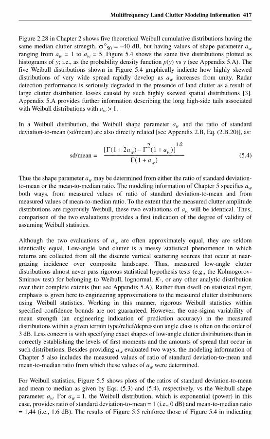
Multifrequency Land Clutter Modeling Information 417

Figure 2.28 in Chapter 2 shows five theoretical Weibull cumulative distributions having thesame median clutter strength, σ°50 = –40 dB, but having values of shape parameter awranging from aw = 1 to aw = 5. Figure 5.4 shows the same five distributions plotted ashistograms of y; i.e., as the probability density function p(y) vs y (see Appendix 5.A). Thefive Weibull distributions shown in Figure 5.4 graphically indicate how highly skeweddistributions of very wide spread rapidly develop as aw increases from unity. Radardetection performance is seriously degraded in the presence of land clutter as a result oflarge clutter distribution losses caused by such highly skewed spatial distributions [3].Appendix 5.A provides further information describing the long high-side tails associatedwith Weibull distributions with aw > 1.

In a Weibull distribution, the Weibull shape parameter aw and the ratio of standarddeviation-to-mean (sd/mean) are also directly related [see Appendix 2.B, Eq. (2.B.20)], as:

sd/mean = (5.4)

Thus the shape parameter aw may be determined from either the ratio of standard deviation-to-mean or the mean-to-median ratio. The modeling information of Chapter 5 specifies awboth ways, from measured values of ratio of standard deviation-to-mean and frommeasured values of mean-to-median ratio. To the extent that the measured clutter amplitudedistributions are rigorously Weibull, these two evaluations of aw will be identical. Thus,comparison of the two evaluations provides a first indication of the degree of validity ofassuming Weibull statistics.

Although the two evaluations of aw are often approximately equal, they are seldomidentically equal. Low-angle land clutter is a messy statistical phenomenon in whichreturns are collected from all the discrete vertical scattering sources that occur at near-grazing incidence over composite landscape. Thus, measured low-angle clutterdistributions almost never pass rigorous statistical hypothesis tests (e.g., the Kolmogorov-Smirnov test) for belonging to Weibull, lognormal, K-, or any other analytic distributionover their complete extents (but see Appendix 5.A). Rather than dwell on statistical rigor,emphasis is given here to engineering approximations to the measured clutter distributionsusing Weibull statistics. Working in this manner, rigorous Weibull statistics withinspecified confidence bounds are not guaranteed. However, the one-sigma variability ofmean strength (an engineering indication of prediction accuracy) in the measureddistributions within a given terrain type/relief/depression angle class is often on the order of3 dB. Less concern is with specifying exact shapes of low-angle clutter distributions than incorrectly establishing the levels of first moments and the amounts of spread that occur insuch distributions. Besides providing aw evaluated two ways, the modeling information ofChapter 5 also includes the measured values of ratio of standard deviation-to-mean andmean-to-median ratio from which these values of aw were determined.

For Weibull statistics, Figure 5.5 shows plots of the ratios of standard deviation-to-meanand mean-to-median as given by Eqs. (5.3) and (5.4), respectively, vs the Weibull shapeparameter aw. For aw = 1, the Weibull distribution, which is exponential (power) in thiscase, provides ratio of standard deviation-to-mean = 1 (i.e., 0 dB) and mean-to-median ratio= 1.44 (i.e., 1.6 dB). The results of Figure 5.5 reinforce those of Figure 5.4 in indicating

Γ 1 2aw+( ) Γ21 aw+( )–[ ]

1 2⁄

Γ 1 aw+( )--------------------------------------------------------------------

418 Multifrequency Land Clutter Modeling Information

how distributions of very wide spread (i.e., large ratios of standard deviation-to-mean andmean-to-median) rapidly arise as aw increases from unity. The plots of Figure 5.5 are usefulas graphical aids to provide quick conversion factors in using the Weibull modelinginformation for aw provided subsequently in Chapter 5. Information comparing the use ofWeibull, lognormal, and K-distributions in the representation of measured clutter amplitudestatistics is provided in Appendix 5.A.

5.2.2 Clutter Model Framework For a given clutter patch, measured clutter histograms were collected and stored for all 20combinations of Phase One radar measurement parameters nominally available (fivefrequencies, two polarizations, two pulse lengths; see Appendix 3.A). Altogether the fileof measured histograms upon which Chapter 5 is based numbers 59,804. Trend analysis ofthese stored data involved sorting out like-classified sets of patches and looking forclustering within sets and separation between sets. This trend analysis led to a generalframework for predicting or modeling clutter in which the fundamental structure is asfollows: (1) Weibull mean strength varies with radar frequency and polarization;(2) Weibull shape parameter aw varies with radar spatial resolution; and (3) both andaw vary with terrain type and depression angle (cf. Section 4.2.2). Note that within thismodeling framework, radar frequency affects but not aw; whereas spatial resolutionaffects aw but not . That is, frequency and resolution decouple in their effects onclutter amplitude statistics. The basic criterion imposed in developing this modelingframework was the degree to which an expected trend or dependency was actually borneout in the measured clutter data. This modeling framework is sufficient to capture all ofthe important trends and dependencies observed in the data.

5.2.2.1 Mean Strength

A key attribute of the first moment or mean strength in a low-angle clutter amplitudedistribution is that it is independent of radar spatial resolution. This fact and its importanceare often unrecognized. It is both theoretically true in power-additive spatial ensembleprocesses and observed to be empirically true in the Phase One measurements. That it istheoretically true was discussed in Chapter 3, Section 3.5.3, and in Chapter 4, Section4.5.4. In the Phase One measurement data, differences in mean strength between high(15 m or 36 m) and low (150 m) range resolution across the complete matrix of repeatsector patches were often less than one decibel (i.e., in the distribution of differences ofmean strength with resolution, the mean difference was 0.8 dB and the median differencewas 0.9 dB; see Figure 3.43).

The fact that the mean is independent of resolution in the modeling construct being utilizedhere has the important benefit of reducing the parametric dimensionality in this construct.Looking ahead to the tabularized modeling information of Chapter 5, if in these tableshad to be further partitioned in several categories of resolution, the number ofmeasurements in any given category would become too small to allow the development ofuseful general trends, and the modeling information would begin to degenerate to trendlesstabularization of data.

The mean is the only attribute of low-angle clutter amplitude distributions that isindependent of resolution. A number of early investigations emphasized the median ratherthan the mean in such distributions, since means usually occur high in the distributions,

σ °wσ °w

σ °wσ °w

σ °w

σ °w

Multifrequency Land Clutter Modeling Information 419

often near the 90-percentile level, driven there by occasional strong returns from discretesources. It was thought that the median might be a better central measure of a discrete-freearea-extensive clutter background. However, attempts to characterize the changing shapesof low-angle clutter amplitude distributions using the median instead of the mean as thecentral measure of each distribution required unwieldy normalization procedures and didnot lead to useful general results, since the median central measure of each distribution aswell as its shape were strongly dependent on resolution [12]. Because the mean occurs highin a distribution is not a reason to discard standard statistical techniques of using the firsttwo moments of any distribution as the best way to begin to bring it under generaldescription.

5.2.2.2 Shape Parameter aw

The shapes of low-angle clutter spatial amplitude distributions are strongly andfundamentally dependent on spatial resolution. However, as with the mean strengths, thereis a similar savings in model dimensionality with the shape parameter. With aw, thissavings is in the fact that the shapes of distributions, as observed in the clutter data, are notvery sensitive to the remaining radar parameters of radar frequency and polarization. Thiskey fact is an empirical observation here that apparently has not been advanced elsewhere.The reason why shapes of clutter amplitude distributions are largely insensitive tofrequency and polarization is that essentially the same set of discrete sources on thelandscape cause the dominant clutter returns, whatever the radar frequency or polarization.This is observed in PPI clutter plots showing the spatial texture of clutter. Insensitivity ofdistribution shape to radar frequency allows bringing to bear the varying Phase Oneazimuth beamwidths with frequency, from 13° at VHF to 1° at X-band, to help provide acombined broad range of spatial resolutions across which to establish trends.

It can be seen in the modeling information of Chapter 5 that, in working across frequencyin this manner to establish trends of spread vs spatial resolution, radar frequency isessentially undetectable in the trends observed. That is, looking ahead to Figure 5.9 andthe following 18 similar figures showing measured results of sd/mean vs A, it is evidentthat the different colored plot symbols in each such figure which correspond to differentfrequency bands contribute much more towards establishing one overall scatter plotthrough which it is most sensible to define one overall regression line, as opposed to fiveindividual scatter plots with five different regression lines. If it were necessary to separateaw with radar frequency and/or polarization, there would not be enough available range inresolution in the Phase One data to properly establish a trend, nor would there be enoughdata to properly fill the matrix.

Thus two important factors upon which the success of the modeling construct employedherein is based are that is dependent on frequency and polarization but is independentof resolution; whereas aw is independent of frequency and polarization but is dependent onresolution—that is, that the important radar parameters decouple in their effects on low-angle clutter spatial amplitude distributions, much reducing the required parametricdimensionality of the model.

σ °w

420 Multifrequency Land Clutter Modeling Information

5.2.3 Derivation of Results

5.2.3.1 Derivation of Results

Like-classified groups of measured clutter histograms were formed in which the classifierswere: terrain type, relief, depression angle, radar frequency band (VHF, UHF, L-, S-, or X-band), and radar polarization (HH or VV). For each like-classified group, the mean clutterstrengths of all the measured clutter histograms within the group were collected, one valueof mean strength per histogram. The median or 50-percentile value from this set of meanstrengths was selected as the representative value of mean strength by which tocharacterize that particular like-classified group of measurements. This 50-percentilevalue of mean clutter strength for each like-classified group of measurements wastabulated as the Weibull mean clutter strength coefficient in Sections 5.3 and 5.4 ofChapter 5. The number of measurements in each like-classified group was also tabulatedin Sections 5.3 and 5.4, as an indication of the degree of generality of each coefficientpresented. Color plots of vs frequency by depression angle regime and polarizationare provided for each terrain type/relief category in Sections 5.3 and 5.4. The like-classified sets of mean clutter strength, upon which the modeling information ofChapter 5 is based, number 864.

Information Underlying . As an example of the derivation of each value of provided as modeling information in what follows, Table 5.2 illustrates the like-classifiedgroups of measured clutter histograms for one terrain type—namely, low-relief forest withdepression angle from 0.25° to 0.75°. The data in Table 5.2 are separated by frequency band(VHF, UHF, L-, S-, X-bands), range resolution (F = fat = 150 m; T = thin = 36 m for VHFand UHF bands, = 15 m for L-, S-, X-bands), and polarization (V = vertical, H = horizontal).

Each line in the table corresponds to one group of like classified histograms. In each line,the following information is provided: the number of histograms in the group (Npts) whichis also the number of available like-classified values of clutter patch mean strength in dB;the median of these dB values (which is what is selected for ); the mean of these dBvalues; the standard deviation of these dB values (i.e., the 1-σ variability of ); themaximum of these dB values (the strongest like-classified patch measured); and theminimum of these dB values (the weakest like-classified patch measured). Looking aheadto Table 5.27 in Section 5.4.3.1, the values shown in the 0.25° to 0.75° lines in the upperand lower subtables of Table 5.27 come from Table 5.2. For example, lines 5 and 6 in Table5.2 provide Npts = 113, 113 (4th column) and = –27.1, –28.0 dB (5th column) forvertical and horizontal polarization, respectively, at VHF. Corresponding information tothat shown in Table 5.2 lies behind all terrain type/depression angle categories for which

values are provided in following Sections 5.3 and 5.4.

5.2.3.2 Derivation of aw Results

The spread in a clutter spatial amplitude distribution as given, for example, by the ratio ofstandard deviation-to-mean or by the mean-to-median ratio, is fundamentally dependenton radar spatial resolution. Radar spatial resolution A (see Section 2.3.1.1) is given by

(5.5)

where

σ °w

σ °w

σ °wσ °w

σ °w

σ °w σ °w

σ °wσ °w

σ °w

σ °w

A r ∆ r ∆θ⋅⋅=

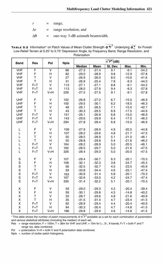
Multifrequency Land Clutter Modeling Information 421

r = range,

∆r = range resolution, and

∆θ = one-way 3-dB azimuth beamwidth.

Table 5.2 Information* on Patch Values of Mean Clutter Strength Underlying for Forest/Low-Relief Terrain at 0.25° to 0.75° Depression Angle, by Frequency Band, Range Resolution, and

Polarization

σ °σ °σ °σ °F4 σ °σ °σ °σ °w

Band Res Pol NptsMedian Mean St. Dev. Max. Min.

VHFVHFVHFVHFVHFVHFVHF

UHFUHFUHFUHFUHFUHFUHF

LLLLLLL

SSSSSSS

XXXXXXX

FFTT

F+TF+TF+T

FFTT

F+TF+TF+T

FFTT

F+TF+TF+T

FFTT

F+TF+TF+T

FFTT

F+TF+TF+T

VHVHVH

V+H

VHVHVH

V+H

VHVHVH

V+H

VHVHVH

V+H

VHVHVH

V+H

86822731

113113226

102100

4943

151143294

1091075555

164162326

107108

5659

163167330

595933359294

186

-27.3-29.0-26.9-26.9-27.1-28.0-27.5

-26.8-29.5-26.1-30.3-26.1-29.6-27.8

-27.9-28.2-28.5-28.8-28.2-28.5-28.4

-29.4-32.1-32.5-33.8-30.6-32.6-31.4

-29.0-30.1-28.7-31.5-28.9-30.3-29.8

-27.4-28.9-26.0-25.4-27.1-27.9-27.5

-27.2-30.1-26.5-29.5-26.9-29.9-28.4

-28.9-29.6-28.9-29.8-28.9-29.7-29.3

-30.7-32.3-32.7-34.4-31.4-33.0-32.2

-29.3-29.8-29.6-31.5-29.4-30.4-29.9

9.19.88.07.88.89.49.1

6.76.27.16.96.86.46.8

4.94.85.15.45.05.05.0

6.33.84.54.65.84.25.1

4.24.54.84.74.44.74.6

-9.1-12.9-10.6

-9.3-9.1-9.3-9.1

-15.0-18.5-15.0-17.5-15.0-17.5-15.0

-20.5-21.7-21.0-21.6-20.5-21.6-20.5

-20.1-24.7-23.5-25.1-20.1-24.7-20.1

-20.4-14.8-21.6-23.4-20.4-14.8-14.8

-54.2-57.8-41.6-44.0-54.2-57.8-57.8

-46.9-46.3-42.7-44.9-46.9-46.3-46.9

-44.8-47.5-46.1-46.2-46.1-47.5-47.5

-70.3-45.4-45.9-47.4-70.3-47.4-70.3

-39.4-40.2-40.9-41.5-40.9-41.5-41.5

* This table shows the number of patch measurements of σ°F4 available as a set for each combination of parameters,and various statistical attributes (including the median) of each set.Res = range resolution; F = 150m; T = 36m for VHF and UHF, = 15m for L-, S-, X-bands; F+T = both F and T

range res. data combined.Pol = polarization; V+H = both V and H polarization data combined.Npts = number of clutter patch histograms.

σ°F4 (dB)

422 Multifrequency Land Clutter Modeling Information

Like-classified groups of measured clutter histograms were formed in which the classifierswere: terrain type, relief, depression angle, range interval, range resolution, and azimuthbeamwidth. Three range intervals were utilized, as: interval 1, 1 to 11.3 km; interval 2, 11.3to 35.7 km; interval 3, range > 35.7 km. The measured clutter histograms are approximatelyequally distributed within these three intervals. Two range resolutions are available, widepulse (i.e., 150 m) or narrow pulse (i.e., 36 m at VHF and UHF, 15 m at L-, S-, and X-bands). Five azimuth beamwidths are available, one per frequency band, as: 13° at VHF,5° at UHF, 3° at L-band, 1° at S- and X-bands. Although S- and X-bands both have ≈1°azimuth beamwidth, they are kept separate in spread analysis classification grouping tokeep the frequency bands separate in the scatter plots (but not in the regression).

For each like-classified group of measured clutter histograms, three parameters werecollected from each of the measured clutter histograms within the group. These threeparameters are: (1) the ratio of standard deviation-to-mean, (2) the mean-to-median ratio,and (3) the value of spatial resolution A applicable for the measurement. The median valuesof each of these three parameters were selected as representative values to characterize thespread in that particular like-classified group of measurements. Spread characterizationutilizing these three parameters proceeded as follows. For each terrain type/relief/depression angle category, two scatter plots were formed. The first scatter plot shows theratio of standard deviation-to-mean vs log10 A. The second scatter plot shows the mean-to-median ratio vs log10 A.

Each plotted point in the first of these scatter plots shows the median value of ratio ofstandard deviation-to-mean vs the median value of log10 A for a particular like-classifiedgroup of measured clutter histograms. A number of these scatter plots of standarddeviation-to-mean vs log10 A are shown in Sections 5.3 and 5.4, one scatter plot for aselected depression angle regime in each terrain type/relief category. Similar to the firstscatter plot, each plotted point in the second scatter plot shows the median value of mean-to-median ratio vs the median value of log10 A for a particular like-classified group ofmeasured clutter histograms. The maximum number of points in a scatter plot is 30(five azimuth beamwidths, two pulse lengths, three range intervals), but little narrow pulsedata is generally available in the third range interval.

Regression analysis was performed in each scatter plot. These regression analysesgenerally show significantly decreasing spread with decreasing resolution (i.e., increasingA) for each terrain type/relief/depression angle category. The regression line for eachscatter plot is provided as modeling information for spread in clutter amplitudedistributions in Chapter 5. The regression line is generally characterized by its values at A =103 m2 and A = 106 m2, with a few noted exceptions.

Modeling information characterizing spread in clutter spatial amplitude distributions basedon regression analysis in the scatter plots is provided two ways: (1) based on measuredratios of standard deviation-to-mean and (2) based on measured mean-to-median ratios. Forboth ways, the regression line values at A = 103 m2 and A = 106 m2 are converted to thecorresponding two values of Weibull shape parameter aw at A = 103 m2 and A = 106 m2 byEquations (5.3) and (5.4). These pairs of values of aw are tabulated by terrain type/relief/depression angle category in Sections 5.3 and 5.4. In addition to the paired values of aw, theunderlying paired values of ratios of standard deviation-to-mean and mean-to-median ratio

Multifrequency Land Clutter Modeling Information 423

are also tabulated. The number of clutter patches and number of measured clutterhistograms that each scatter plot (i.e., regression analysis) is based on is also tabulated.

This tabulated modeling information for Weibull shape parameter aw is used as follows.First, the spatial resolution A of the radar under study is calculated at the terrain point underconsideration. Then linear interpolation on log10 A between the values of aw at A = 103 m2

and A = 106 m2 for the appropriate terrain type/relief/depression angle category isperformed to obtain the value of aw at the radar spatial resolution A in question. Preferenceis given to the tabulated values of aw based on measured ratios of standard deviation-to-mean. The additional provision of tabulated values of aw based on measured mean-to-median ratios provides a first indication of the degree of validity of modeling theunderlying measured data with Weibull statistics, based on how closely aw computed frommeasured ratios of standard deviation-to-mean approximates aw computed from measuredmean-to-median ratios. The like-classified sets of measured clutter histograms, upon whichthe aw modeling information of Chapter 5 is based, number 1,510. Note that these aredifferent sets than those upon which the modeling information is based.

Information Underlying aw. As described above, the aw values provided as modelinginformation in what follows come from regression in scatter plots. Two scatter plots wereformed: one of sd/mean (dB) vs log10 A; the other of mean/median (dB) vs log10 A. Eachscatter plot comes from like-classified groups of measured clutter histograms. As anexample of the information underlying the two scatter plots for low-relief forest withdepression angle from 0.25° to 0.75°, Table 5.3 is shown here in three parallel parts. Parts(a), (b), and (c) show results for sd/mean (dB), mean/median (dB), and patch mid-range(km), respectively.

Consider first Table 5.3(a) for sd/mean (dB). The data in Table 5.3(a) are separated byfrequency band (VHF, UHF, L, S, X), range resolution (Fat or Thin), and range interval (1,2, or 3, as described previously). Each line in the table corresponds to one group of like-classified histograms and one point in the corresponding scatter plot—note that the groupsare different from those of Table 5.2. In each line of Table 5.3(a), the following informationis provided: the median value of mid-range cell size A for the group (shown under X as X =log10 A and A = in m2); the number of histograms in the group (Npts), whichis also the number of available like-classified values of ratio of sd/mean (dB), one fromeach clutter patch histogram; the median of these dB values of sd/mean (which forms theordinate of the point in the scatter plot corresponding to this line); the mean of the dBvalues of sd/mean; the standard deviation of the dB values of sd/mean (i.e., the vertical 1-σvariability of this point in the scatter plot); the maximum of these dB values of sd/mean(i.e., the maximum patch value of sd/mean in this group); and the minimum of these dBvalues of mean/median. Thus, each line in Table 5.3(a) corresponds to the ordinate of agiven point in a given scatter plot. For example, the scatter plot for low-relief forest, 0.0° to0.25° depression angle is shown as Figure 5.27 in Section 5.4.3.2 (note: the plotcorresponding to the 0.25° to 0.75° depression angle regime of Table 5.3 is not shown).

Table 5.3(b) is similar to Table 5.3(a) except Table 5.3(b) provides underlying informationfor the ordinate of the plotted points in the scatter plots of mean/median (dB) vs log10 A.Examples of the mean/median scatter plots are not shown in this book; they appear similarto the sd/mean scatter plots, except that they employ a different y-scale.

σ °w

r ∆r ∆θ⋅⋅

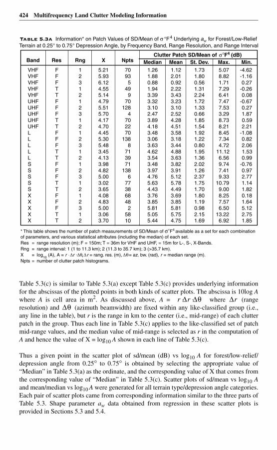
424 Multifrequency Land Clutter Modeling Information

Table 5.3(c) is similar to Table 5.3(a) except Table 5.3(c) provides underlying informationfor the abscissas of the plotted points in both kinds of scatter plots. The abscissa is 10log Awhere A is cell area in m2. As discussed above, A = where (rangeresolution) and (azimuth beamwidth) are fixed within any like-classified group (i.e.,any line in the table), but r is the range in km to the center (i.e., mid-range) of each clutterpatch in the group. Thus each line in Table 5.3(c) applies to the like-classified set of patchmid-range values, and the median value of mid-range is selected as r in the computation ofA and hence the value of X = log10 A shown in each line of Table 5.3(c).

Thus a given point in the scatter plot of sd/mean (dB) vs log10 A for forest/low-relief/depression angle from 0.25° to 0.75° is obtained by selecting the appropriate value of“Median” in Table 5.3(a) as the ordinate, and the corresponding value of X that comes fromthe corresponding value of “Median” in Table 5.3(c). Scatter plots of sd/mean vs log10 Aand mean/median vs log10 A were generated for all terrain type/depression angle categories.Each pair of scatter plots came from corresponding information similar to the three parts ofTable 5.3. Shape parameter aw data obtained from regression in these scatter plots isprovided in Sections 5.3 and 5.4.

Table 5.3a Information* on Patch Values of SD/Mean of σ °F4 Underlying aw for Forest/Low-Relief Terrain at 0.25° to 0.75° Depression Angle, by Frequency Band, Range Resolution, and Range Interval

* This table shows the number of patch measurements of SD/Mean of σ°F4 available as a set for each combinationof parameters, and various statistical attributes (including the median) of each set.Res = range resolution (m); F = 150m; T = 36m for VHF and UHF, = 15m for L-, S-, X-Bands.Rng = range interval: 1 (1 to 11.3 km); 2 (11.3 to 35.7 km); 3 (>35.7 km).X = log

10 (A), A = r ⋅ r ⋅ , r = rang. res. (m), = az. bw. (rad), r = median range (m).

Npts = number of clutter patch histograms.

Clutter Patch SD/Mean of F4 (dB)Band Res Rng X Npts Median Mean St. Dev. Max. Min.VHFVHFVHFVHFVHFUHFUHFUHFUHFUHFLLLLLSSSSSXXXXX

FFFTTFFFTTFFFTTFFFTTFFFTT

1231212312123121231212312

5.215.936.124.555.144.795.515.704.174.704.455.305.483.454.133.984.825.003.023.654.084.835.003.063.70

70935

499

70128

4702270

1388

713971

1386

773868482

5810

1.261.880.881.943.393.323.102.473.894.183.483.063.634.623.543.483.974.765.634.433.763.855.815.055.44

1.122.010.922.223.433.233.102.524.284.513.583.183.444.883.633.823.915.125.784.493.693.855.815.754.75

1.731.800.561.312.241.721.330.661.851.541.921.220.801.951.362.021.262.371.751.701.801.190.982.151.69

5.078.821.717.296.417.477.533.298.738.218.457.344.72

11.126.569.747.419.33

10.799.008.257.576.50

13.226.92

-4.62-1.160.27

-0.260.08

-0.670.271.870.592.21

-1.080.822.061.530.99

-0.760.972.771.141.820.181.645.122.751.85

r ∆r ∆θ⋅⋅ ∆r∆θ

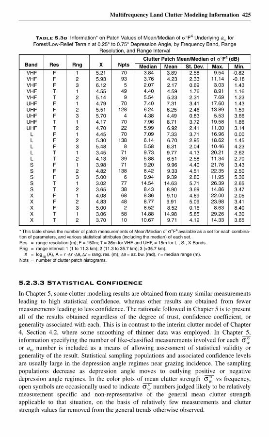
Multifrequency Land Clutter Modeling Information 425

5.2.3.3 Statistical Confidence

In Chapter 5, some clutter modeling results are obtained from many similar measurementsleading to high statistical confidence, whereas other results are obtained from fewermeasurements leading to less confidence. The rationale followed in Chapter 5 is to presentall of the results obtained regardless of the degree of trust, confidence coefficient, orgenerality associated with each. This is in contrast to the interim clutter model of Chapter4, Section 4.2, where some smoothing of thinner data was employed. In Chapter 5,information specifying the number of like-classified measurements involved for each or aw number is included as a means of allowing assessment of statistical validity orgenerality of the result. Statistical sampling populations and associated confidence levelsare usually large in the depression angle regimes near grazing incidence. The samplingpopulations decrease as depression angle moves to outlying positive or negativedepression angle regimes. In the color plots of mean clutter strength vs frequency,open symbols are occasionally used to indicate numbers judged likely to be relativelymeasurement specific and non-representative of the general mean clutter strengthapplicable to that situation, on the basis of relatively few measurements and clutterstrength values far removed from the general trends otherwise observed.

Table 5.3b Information* on Patch Values of Mean/Median of σ°F4 Underlying aw for Forest/Low-Relief Terrain at 0.25° to 0.75° Depression Angle, by Frequency Band, Range

Resolution, and Range Interval

Clutter Patch Mean/Median of F4 (dB) Band Res Rng X Npts Median Mean St. Dev. Max. Min.VHFVHFVHFVHFVHFUHFUHFUHFUHFUHF

LLLLLSSSSSXXXXX

FFFTTFFFTTFFFTTFFFTTFFFTT

1231212312123121231212312

5.215.936.124.555.144.795.515.704.174.704.455.305.483.454.133.984.825.003.023.654.084.835.003.063.70

3.894.232.174.595.237.316.254.498.716.927.336.706.319.776.519.969.339.39

14.638.909.109.918.52

14.989.71

2.582.330.691.762.313.412.460.833.722.413.712.952.044.132.584.404.512.805.713.694.695.090.165.854.19

-0.82-0.181.431.161.231.431.593.661.863.140.001.454.232.622.703.432.505.362.653.472.053.418.404.303.65

* This table shows the number of patch measurements of Mean/Median of F4 available as a set for each combina-tion of parameters, and various statistical attributes (including the median) of each set.Res = range resolution (m); F = 150m; T = 36m for VHF and UHF, = 15m for L-, S-, X-Bands.Rng = range interval: 1 (1 to 11.3 km); 2 (11.3 to 35.7 km); 3 (>35.7 km). X = log

10 (A), A = r ⋅ r ⋅ , r = rang. res. (m), = az. bw. (rad), r = median range (m).

Npts = number of clutter patch histograms.

70935

499

70128

4702270

1388

713971

1386

773868482

5810

3.843.762.074.405.547.406.244.387.965.997.096.145.589.735.889.208.429.94

14.548.438.368.778.52

14.8810.67

9.5411.143.038.917.69

17.6013.895.53

19.5811.0016.9618.6210.4620.2111.3421.7622.3511.9526.3914.8622.0023.988.63

29.2614.33

σ °w

σ °wσ °w

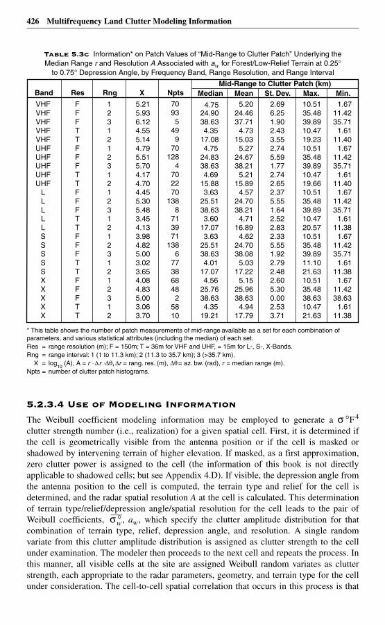
426 Multifrequency Land Clutter Modeling Information

5.2.3.4 Use of Modeling Information

The Weibull coefficient modeling information may be employed to generate a σ °F4

clutter strength number (i.e., realization) for a given spatial cell. First, it is determined ifthe cell is geometrically visible from the antenna position or if the cell is masked orshadowed by intervening terrain of higher elevation. If masked, as a first approximation,zero clutter power is assigned to the cell (the information of this book is not directlyapplicable to shadowed cells; but see Appendix 4.D). If visible, the depression angle fromthe antenna position to the cell is computed, the terrain type and relief for the cell isdetermined, and the radar spatial resolution A at the cell is calculated. This determinationof terrain type/relief/depression angle/spatial resolution for the cell leads to the pair ofWeibull coefficients, , aw, which specify the clutter amplitude distribution for thatcombination of terrain type, relief, depression angle, and resolution. A single randomvariate from this clutter amplitude distribution is assigned as clutter strength to the cellunder examination. The modeler then proceeds to the next cell and repeats the process. Inthis manner, all visible cells at the site are assigned Weibull random variates as clutterstrength, each appropriate to the radar parameters, geometry, and terrain type for the cellunder consideration. The cell-to-cell spatial correlation that occurs in this process is that

Table 5.3c Information* on Patch Values of “Mid-Range to Clutter Patch” Underlying the Median Range r and Resolution A Associated with aw for Forest/Low-Relief Terrain at 0.25°

to 0.75° Depression Angle, by Frequency Band, Range Resolution, and Range Interval

Mid-Range to Clutter Patch (km)Band Res Rng X Npts Median Mean St. Dev. Max. Min.VHFVHFVHFVHFVHFUHFUHFUHFUHFUHF

LLLLLSSSSSXXXXX

FFFTTFFFTTFFFTTFFFTTFFFTT

1231212312123121231212312

5.215.936.124.555.144.795.515.704.174.704.455.305.483.454.133.984.825.003.023.654.084.835.003.063.70

4.7524.9038.634.35

17.084.75

24.8338.634.69

15.883.63

25.5138.633.60

17.073.63

25.5138.634.01

17.074.56

25.7638.634.35

19.21

5.2024.4637.71

4.7315.03

5.2724.6738.21

5.2115.89

4.5724.7038.21

4.7116.89

4.6224.7038.08

5.0317.22

5.1525.9638.63

4.9417.79

2.696.251.902.433.552.745.591.772.742.652.375.551.642.522.832.335.551.922.792.482.605.300.002.533.71

10.5135.4839.8910.4719.2310.5135.4839.8910.4719.6610.5135.4839.8910.4720.5710.5135.4839.8911.1021.6310.5135.4838.6310.4721.63

1.6711.4235.71

1.6111.40

1.6711.4235.71

1.6111.40

1.6711.4235.71

1.6111.38

1.6711.4235.71

1.6111.38

1.6711.4238.63

1.6111.38

* This table shows the number of patch measurements of mid-range available as a set for each combination ofparameters, and various statistical attributes (including the median) of each set.Res = range resolution (m); F = 150m; T = 36m for VHF and UHF, = 15m for L-, S-, X-Bands.Rng = range interval: 1 (1 to 11.3 km); 2 (11.3 to 35.7 km); 3 (>35.7 km). X = log

10 (A), A = r ⋅ r ⋅ , r = rang. res. (m), = az. bw. (rad), r = median range (m).

Npts = number of clutter patch histograms.

70935

499

70128

4702270

1388

713971

1386

773868482

5810

σ °w

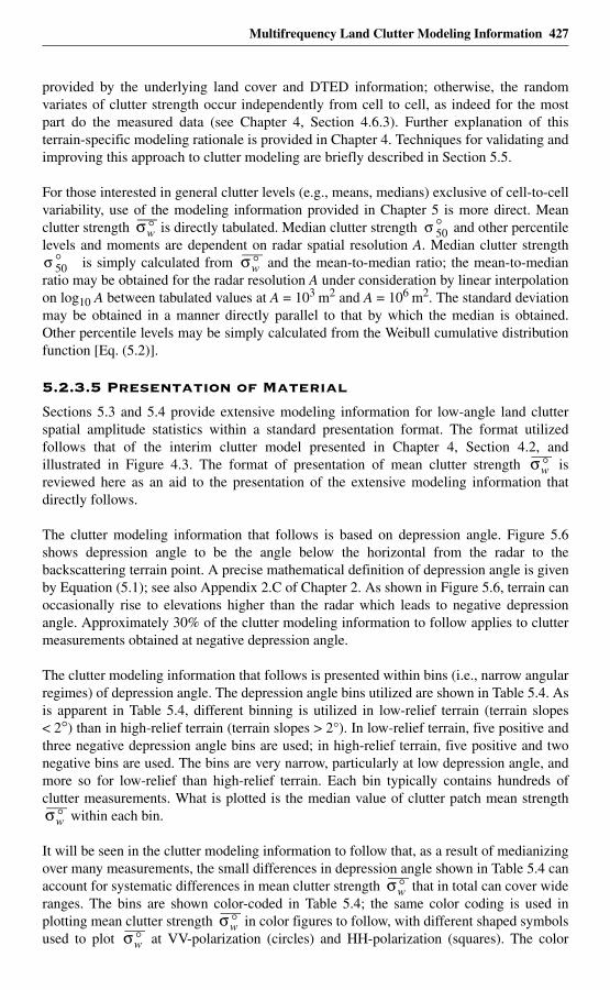
Multifrequency Land Clutter Modeling Information 427

provided by the underlying land cover and DTED information; otherwise, the randomvariates of clutter strength occur independently from cell to cell, as indeed for the mostpart do the measured data (see Chapter 4, Section 4.6.3). Further explanation of thisterrain-specific modeling rationale is provided in Chapter 4. Techniques for validating andimproving this approach to clutter modeling are briefly described in Section 5.5.

For those interested in general clutter levels (e.g., means, medians) exclusive of cell-to-cellvariability, use of the modeling information provided in Chapter 5 is more direct. Meanclutter strength is directly tabulated. Median clutter strength and other percentilelevels and moments are dependent on radar spatial resolution A. Median clutter strength

is simply calculated from and the mean-to-median ratio; the mean-to-medianratio may be obtained for the radar resolution A under consideration by linear interpolationon log10 A between tabulated values at A = 103 m2 and A = 106 m2. The standard deviationmay be obtained in a manner directly parallel to that by which the median is obtained.Other percentile levels may be simply calculated from the Weibull cumulative distributionfunction [Eq. (5.2)].

5.2.3.5 Presentation of Material

Sections 5.3 and 5.4 provide extensive modeling information for low-angle land clutterspatial amplitude statistics within a standard presentation format. The format utilizedfollows that of the interim clutter model presented in Chapter 4, Section 4.2, andillustrated in Figure 4.3. The format of presentation of mean clutter strength isreviewed here as an aid to the presentation of the extensive modeling information thatdirectly follows.

The clutter modeling information that follows is based on depression angle. Figure 5.6shows depression angle to be the angle below the horizontal from the radar to thebackscattering terrain point. A precise mathematical definition of depression angle is givenby Equation (5.1); see also Appendix 2.C of Chapter 2. As shown in Figure 5.6, terrain canoccasionally rise to elevations higher than the radar which leads to negative depressionangle. Approximately 30% of the clutter modeling information to follow applies to cluttermeasurements obtained at negative depression angle.

The clutter modeling information that follows is presented within bins (i.e., narrow angularregimes) of depression angle. The depression angle bins utilized are shown in Table 5.4. Asis apparent in Table 5.4, different binning is utilized in low-relief terrain (terrain slopes< 2°) than in high-relief terrain (terrain slopes > 2°). In low-relief terrain, five positive andthree negative depression angle bins are used; in high-relief terrain, five positive and twonegative bins are used. The bins are very narrow, particularly at low depression angle, andmore so for low-relief than high-relief terrain. Each bin typically contains hundreds ofclutter measurements. What is plotted is the median value of clutter patch mean strength

within each bin.

It will be seen in the clutter modeling information to follow that, as a result of medianizingover many measurements, the small differences in depression angle shown in Table 5.4 canaccount for systematic differences in mean clutter strength that in total can cover wideranges. The bins are shown color-coded in Table 5.4; the same color coding is used inplotting mean clutter strength in color figures to follow, with different shaped symbolsused to plot at VV-polarization (circles) and HH-polarization (squares). The color

σ °w σ 50°

σ 50° σ °w

σ °w

σ °w

σ °w

σ °wσ °w

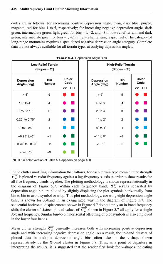
428 Multifrequency Land Clutter Modeling Information

codes are as follows: for increasing positive depression angle, cyan, dark blue, purple,magenta, red for bins 1 to 5, respectively; for increasing negative depression angle, darkgreen, intermediate green, light green for bins –1, –2, and –3 in low-relief terrain, and darkgreen, intermediate green for bins –1, –2 in high-relief terrain, respectively. The category oflong-range mountains requires a specialized negative depression angle category. Completedata are not always available for all terrain types at outlying depression angles.

In the clutter modeling information that follows, for each terrain type mean clutter strength is plotted vs radar frequency against a log-frequency x-axis in order to show results for

all five frequency bands together. The plotting methodology is shown representationally inthe diagram of Figure 5.7. Within each frequency band, results separated bydepression angle bin are plotted by slightly displacing the plot symbols horizontally frombin to bin to avoid symbol overlap. This plot methodology, covering eight depression anglebins, is shown for X-band in an exaggerated way in the diagram of Figure 5.7. Thesequential horizontal displacements shown in Figure 5.7 do not imply an in-band frequencyshift; the cluster of sixteen plotted values of shown in Figure 5.7 all apply for a singleX-band frequency. Similar bin-to-bin horizontal offsetting of plot symbols is also employedin the lower four bands.

Mean clutter strength generally increases both with increasing positive depressionangle and with increasing negative depression angle. As a result, the in-band clusters ofplotted data in multiple depression angle bins often take on the v-shape shownrepresentatively by the X-band cluster in Figure 5.7. Thus, as a point of departure ininterpreting the results, it is suggested that the reader first look for v-shapes indicating

Table 5.4 Depression Angle Bins

NOTE: A color version of Table 5.4 appears on page 450.

Low-Relief Terrain

(Slopes < 2˚)

DepressionAngle (deg)

BinNumber

ColorCode

VV HH

> 4˚

1.5˚ to 4˚

0.75˚ to 1.5˚

0.25˚ to 0.75˚

0˚ to 0.25˚

–0.25˚ to 0˚

–0.75˚ to –0.25˚

< – 0.75˚

5

4

3

2

1

–1

–2

–3

High-Relief Terrain

(Slopes > 2˚)

> 6˚

4˚ to 6˚

2˚ to 4˚

1˚ to 2˚

0˚ to 1˚

–1˚ to 0˚

< –1˚

5

4

3

2

1

–1

–2

DepressionAngle (deg)

BinNumber

ColorCode

VV HH

σ °w

σ °w

σ °w

σ °w

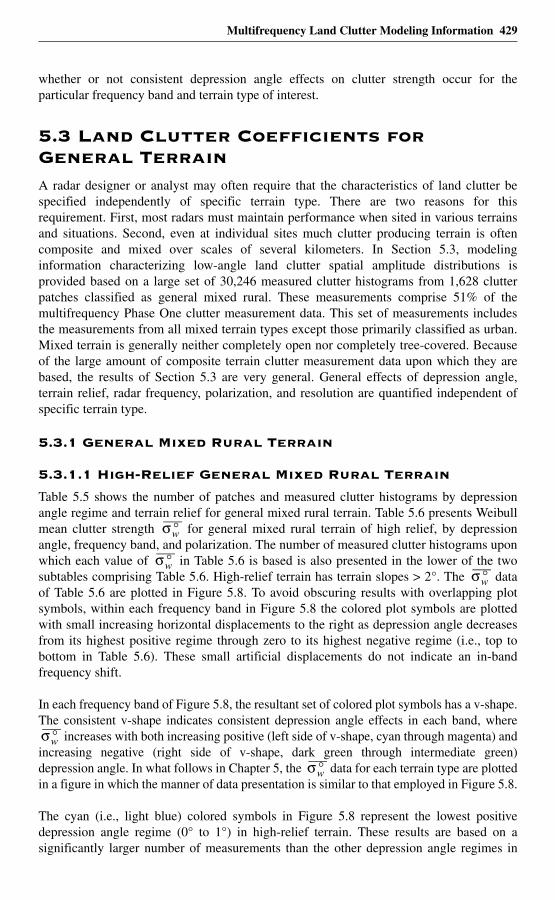
Multifrequency Land Clutter Modeling Information 429

whether or not consistent depression angle effects on clutter strength occur for theparticular frequency band and terrain type of interest.

5.3 Land Clutter Coefficients for General TerrainA radar designer or analyst may often require that the characteristics of land clutter bespecified independently of specific terrain type. There are two reasons for thisrequirement. First, most radars must maintain performance when sited in various terrainsand situations. Second, even at individual sites much clutter producing terrain is oftencomposite and mixed over scales of several kilometers. In Section 5.3, modelinginformation characterizing low-angle land clutter spatial amplitude distributions isprovided based on a large set of 30,246 measured clutter histograms from 1,628 clutterpatches classified as general mixed rural. These measurements comprise 51% of themultifrequency Phase One clutter measurement data. This set of measurements includesthe measurements from all mixed terrain types except those primarily classified as urban.Mixed terrain is generally neither completely open nor completely tree-covered. Becauseof the large amount of composite terrain clutter measurement data upon which they arebased, the results of Section 5.3 are very general. General effects of depression angle,terrain relief, radar frequency, polarization, and resolution are quantified independent ofspecific terrain type.

5.3.1 General Mixed Rural Terrain

5.3.1.1 High-Relief General Mixed Rural Terrain

Table 5.5 shows the number of patches and measured clutter histograms by depressionangle regime and terrain relief for general mixed rural terrain. Table 5.6 presents Weibullmean clutter strength for general mixed rural terrain of high relief, by depressionangle, frequency band, and polarization. The number of measured clutter histograms uponwhich each value of in Table 5.6 is based is also presented in the lower of the twosubtables comprising Table 5.6. High-relief terrain has terrain slopes > 2°. The dataof Table 5.6 are plotted in Figure 5.8. To avoid obscuring results with overlapping plotsymbols, within each frequency band in Figure 5.8 the colored plot symbols are plottedwith small increasing horizontal displacements to the right as depression angle decreasesfrom its highest positive regime through zero to its highest negative regime (i.e., top tobottom in Table 5.6). These small artificial displacements do not indicate an in-bandfrequency shift.

In each frequency band of Figure 5.8, the resultant set of colored plot symbols has a v-shape.The consistent v-shape indicates consistent depression angle effects in each band, where

increases with both increasing positive (left side of v-shape, cyan through magenta) andincreasing negative (right side of v-shape, dark green through intermediate green)depression angle. In what follows in Chapter 5, the data for each terrain type are plottedin a figure in which the manner of data presentation is similar to that employed in Figure 5.8.

The cyan (i.e., light blue) colored symbols in Figure 5.8 represent the lowest positivedepression angle regime (0° to 1°) in high-relief terrain. These results are based on asignificantly larger number of measurements than the other depression angle regimes in

σ °w

σ °wσ °w

σ °w

σ °w

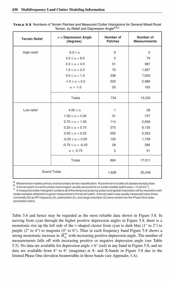
430 Multifrequency Land Clutter Modeling Information

Table 5.6 and hence may be regarded as the most reliable data shown in Figure 5.8. Inmoving from cyan through the higher positive depression angles in Figure 5.8, there is amonotonic rise up the left side of the v-shaped cluster from cyan to dark blue (1° to 2°) topurple (2° to 4°) to magenta (4° to 6°). Thus in each frequency band Figure 5.8 shows astrong monotonic increase in with increasing positive depression angle. The number ofmeasurements falls off with increasing positive or negative depression angle (see Table5.5). No data are available for depression angle > 6° (red) in any band in Figure 5.8, and nodata are available from 4° to 6° (magenta) at S- and X-bands in Figure 5.8 due to thelimited Phase One elevation beamwidths in those bands (see Appendix 3.A).

Table 5.5 Numbers of Terrain Patches and Measured Clutter Histograms for General Mixed Rural Terrain, by Relief and Depression Anglea,b,c

a Mixed terrain implies primary and secondary terrain classification. Rural terrain includes all classes except urban.b A terrain patch is a land surface macroregion usually several kms on a side (median patch area = 12.62 km2).c A measured clutter histogram contains all of the temporal (pulse by pulse) and spatial (resolution cell by resolution cell) clutter samples obtained in a given measurement of a terrain patch. A terrain patch was usually measured many times(nominally 20) as RF frequency (5), polarization (2), and range resolution (2) were varied over the Phase One radarparameter matrix.

Terrain Relief

Totals

High-relief

734 13,235

6.0 ≤ �

4.0 ≤ � < 6.0

2.0 ≤ � < 4.0

1.0 ≤ � < 2.0

0.0 ≤ � < 1.0

-1.0 ≤ � < 0.0

� < -1.0

0

5

51

70

338

250

20

0

79

987

1,997

7,003

2,986

183

Totals

Low-relief

Grand Totals

894 17,011

1,628 30,246

4.00 ≤ �

1.50 ≤ � < 4.00

0.75 ≤ � < 1.50

0.25 ≤ � < 0.75

0.00 ≤ � < 0.25

-0.25 ≤ � < 0.00

-0.75 ≤ � < -0.25

� < -0.75

1

31

114

275

292

150

28

3

28

747

2,659

6,130

5,353

1,758

285

51

� = Depression Angle(degrees)

Number ofPatches

Number ofMeasurements

σ °w

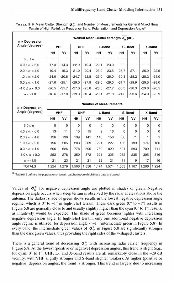
Multifrequency Land Clutter Modeling Information 431

Values of for negative depression angle are plotted in shades of green. Negativedepression angle occurs when steep terrain is observed by the radar at elevations above theantenna. The darkest shade of green shows results in the lowest negative depression angleregime, which is 0° to –1° in high-relief terrain. These dark green (0° to –1°) results inFigure 5.8 are generally close to and usually slightly higher than the cyan (0° to 1°) results,as intuitively would be expected. The shade of green becomes lighter with increasingnegative depression angle. In high-relief terrain, only one additional negative depressionangle regime is utilized, for depression angle < –1° (intermediate green in Figure 5.8). Inevery band, the intermediate green values of in Figure 5.8 are significantly strongerthan the dark green values, thus providing the right sides of the v-shaped clusters.

There is a general trend of decreasing with increasing radar carrier frequency inFigure 5.8. At the lowest (positive or negative) depression angles, this trend is slight (e.g.,for cyan, 0° to 1°, UHF, L-, and X-band results are all remarkably close in the –29 dBvicinity, with VHF slightly stronger and S-band slighter weaker). At higher (positive ornegative) depression angles, the trend is stronger. This trend is largely due to increasing

Table 5.6 Mean Clutter Strength and Number of Measurements for General Mixed Rural Terrain of High Relief, by Frequency Band, Polarization, and Depression Anglea

σ °σ °σ °σ °w

Weibull Mean Clutter Strength w (dB)σ°

HH VV HH VV HH VV HH VV HH VV

- - - - - - - - - - - - - - - - - - - - - - - - - - - - - - - - - - - - - - - -

- - - - - - - - - - - - - - - -

a Table 5.5 defines the population of terrain patches upon which these data are based.

� = DepressionAngle (degrees)

� = DepressionAngle (degrees)

Number of Measurements

UHF L-Band S-Band X-Band

VV HH VV HH VV HH VV HH VV HH

VHF

UHF L-Band S-Band X-BandVHF

6.0 ≤ �

4.0 ≤ � < 6.0

2.0 ≤ � < 4.0

1.0 ≤ � < 2.0

0.0 ≤ � < 1.0

-1.0 ≤ � < 0.0

� < -1.0

-17.3

-19.4

-24.0

-27.6

-26.5

-16.6

-22.5

-24.0

-28.0

-28.5

-25.9

-25.9

-25.2

-29.5

-29.6

-24.9

-27.1

-28.2

-29.9

-28.3

-23.6

-28.7

-30.3

-31.7

-30.3

-24.6

-23.0

-23.5

-26.0

-29.0

-27.7

-21.0

-22.1

-23.0

-26.0

-29.0

-26.6

-23.1

-19.4

-20.4

-22.8

-27.9

-25.8

-16.4

-22.9

-21.0

-24.7

-29.0

-27.0

-19.8

-14.3

-15.3

-20.6

-25.1

-21.7

-17.0

6.0 ≤ �

4.0 ≤ � < 6.0

2.0 ≤ � < 4.0

1.0 ≤ � < 2.0

0.0 ≤ � < 1.0

-1.0 ≤ � < 0.0

� < -1.0

TOTALS

0

13

136

196

606

252

21

1,224

0

0

1

180

711

316

16

1,224

0

0

1

174

709

305

17

1,206

0

0

71

199

593

235

9

1,107

0

0

66

183

591

232

11

1,083

0

16

156

227

829

325

21

1,574

0

9

140

221

760

321

23

1,474

0

15

141

209

800

372

21

1,558

0

15

139

203

778

350

21

1,506

0

11

136

205

626

278

23

1,279

σ °w

σ °w

σ °w

432 Multifrequency Land Clutter Modeling Information

absorption of radio frequency (RF) power from the incident radar wave by tree foliage,VHF to S-band (see Chapter 3). Mixed rural terrain of high relief has a larger componentof trees than at low relief. At the highest positive depression angles (magenta and purple)in Figure 5.8, the variation of with radar frequency f VHF to S-band is approximately

(f) ∝ f -0.94. In the historical literature, what little information is available on thesubject usually suggests a slight trend of increasing clutter strength with increasing radarfrequency, for example, (f) ∝ f 1/2 or (f) ∝ f [2–5]. Thus the trend of decreasingclutter strength with increasing radar frequency seen in many of the Phase One high-angle forest measurements is relatively unexpected. Note that at all positive depressionangles in Figure 5.8, the trend of decreasing with increasing radar frequency fromVHF to S-band reverses from S-band to X-band. That is, at all positive depression anglesthere is an S-band dip between L-band and X-band in Figure 5.8, indicating that over therange of frequencies shown, maximum RF absorption occurs at S-band. It is probably notentirely coincidental that S-band is also the frequency band in which the commonhousehold microwave oven operates (at 2.45 GHz). In Figure 5.8, the differences withpolarization are generally small, on the order of several dB or less, with verticalpolarization (VV) almost always stronger than horizontal (HH).

Table 5.7 presents the Weibull shape parameter aw and ratios of standard deviation-to-meanand mean-to-median for general mixed rural terrain of high relief, by depression angle andradar spatial resolution. Whereas the information of Table 5.6 specifies the mean or firstmoment of the clutter spatial amplitude distribution, the information of Table 5.7 specifiesthe spread or variability in the distribution as determined by the second moment or otherderivative quantities. Table 5.5 shows the number of terrain patches and number ofmeasured clutter histograms for general mixed rural terrain of high relief, broken down bydepression angle in a parallel manner to that of Table 5.7; that is, the statistical populationsunderlying the data of Table 5.7 are available in Table 5.5. The numbers of measured clutterhistograms in Table 5.5 are further broken down by frequency band and polarization inTable 5.6. Table 5.5 shows no data available for depression angle > 6° for general mixedrural terrain of high relief. Generally, there is little Phase One data available at such a highdepression angle, although Section 5.4 shows that there is one high-relief forest clutterpatch and six mountain clutter patches at depression angles > 6°.

In Table 5.7, aw is calculated two ways: (1) from the ratio of standard deviation-to-meanand (2) from the mean-to-median ratio. In Table 5.7, and in general throughout Chapter 5,no major systematic difference results between these two methods of calculation of aw, or,including as a third alternative, in the aw that comes from the least-mean-squares best-fitting true Weibull distribution that is matched to the measured distribution over a largecentral part (i.e., noise level to 0.999 cumulative probability) of the measured distribution.However, aw results by two different methods of calculation are shown in Table 5.7 and inall similar tables throughout Chapter 5 as a first indication of the degree to which Weibullstatistics approximate the characteristics of the measured distributions; if the measureddistributions were exactly Weibull, the two different methods of calculation of aw wouldyield identical results.

Each pair of aw numbers in Table 5.7 comes from a scatter plot in which each individualpoint plotted shows the median value of spread vs the median value of spatial resolution ina group of like-classified measured clutter histograms. For example, for Table 5.7 thestandard deviation-to-mean scatter plot for the 2° to 4° depression angle regime is shown in

σ °wσ °w

σ °w σ °w

σ °w

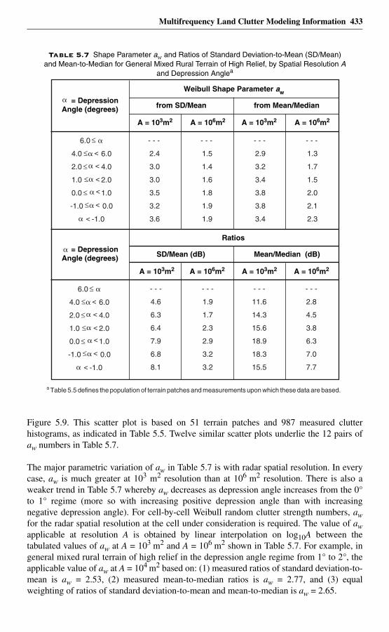
Multifrequency Land Clutter Modeling Information 433

Figure 5.9. This scatter plot is based on 51 terrain patches and 987 measured clutterhistograms, as indicated in Table 5.5. Twelve similar scatter plots underlie the 12 pairs ofaw numbers in Table 5.7.

The major parametric variation of aw in Table 5.7 is with radar spatial resolution. In everycase, aw is much greater at 103 m2 resolution than at 106 m2 resolution. There is also aweaker trend in Table 5.7 whereby aw decreases as depression angle increases from the 0°to 1° regime (more so with increasing positive depression angle than with increasingnegative depression angle). For cell-by-cell Weibull random clutter strength numbers, awfor the radar spatial resolution at the cell under consideration is required. The value of awapplicable at resolution A is obtained by linear interpolation on log10A between thetabulated values of aw at A = 103 m2 and A = 106 m2 shown in Table 5.7. For example, ingeneral mixed rural terrain of high relief in the depression angle regime from 1° to 2°, theapplicable value of aw at A = 104 m2 based on: (1) measured ratios of standard deviation-to-mean is aw = 2.53, (2) measured mean-to-median ratios is aw = 2.77, and (3) equalweighting of ratios of standard deviation-to-mean and mean-to-median is aw = 2.65.

Table 5.7 Shape Parameter aw and Ratios of Standard Deviation-to-Mean (SD/Mean) and Mean-to-Median for General Mixed Rural Terrain of High Relief, by Spatial Resolution A

and Depression Anglea

a Table 5.5 defines the population of terrain patches and measurements upon which these data are based.

Weibull Shape Parameter aw

A = 103m2

= DepressionAngle (degrees) from SD/Mean from Mean/Median

6.0

4.0 6.0

2.0 4.0

1.0 2.0

0.0 1.0

-1.0 0.0

-1.0

- - -

2.4

3.0

3.0

3.5

3.2

3.6

A = 106m2

- - -

1.5

1.4

1.6

1.8

1.9

1.9

A = 103m2

- - -

2.9

3.2

3.4

3.8

3.8

3.4

A = 106m2

Ratios

A = 103m2

= DepressionAngle (degrees) SD/Mean (dB) Mean/Median (dB)

A = 106m2 A = 103m2 A = 106m2

- - -

1.3

1.7

1.5

2.0

2.1

2.3

- - -

4.6

6.3

6.4

7.9

6.8

8.1

- - -

1.9

1.7

2.3

2.9

3.2

3.2

- - -

11.6

14.3

15.6

18.9

18.3

15.5

- - -

2.8

4.5

3.8

6.3

7.0

7.7

≤ �

<

<

<

<

<

<

�

�

�

�

�

�

�

�

≤

≤

≤

≤

≤

6.0

4.0 6.0

2.0 4.0

1.0 2.0

0.0 1.0

-1.0 0.0

-1.0

≤ �

<

<

<

<

<

<

�

�

�

�

�

�

≤

≤

≤

≤

≤

434 Multifrequency Land Clutter Modeling Information

The lower subtable of Table 5.7 shows the ratios of standard deviation-to-mean and mean-to-median from which the aw numbers in the upper subtable come. The large spreads inlow-angle land clutter spatial amplitude distributions at high spatial resolution are perhapsmore dramatically evidenced by these lower numbers (e.g., mean-to-median ratio =18.9 dB at 103 m2, compared to 6.3 dB at 106 m2, Table 5.7, depression angle regime from1° to 2°). Figure 5.5 allows quick conversion between the numbers in the upper and lowersubtables of Table 5.7, and similar tables throughout Chapter 5. Interpolation in these lowernumbers directly yields general second moment or median values at the spatial resolutionunder consideration. For example, at A = 104 m2, for general mixed rural terrain of highrelief in the 1° to 2° depression angle regime, the ratio of standard deviation-to-mean is5.0 dB and the mean-to-median ratio is 11.7 dB. The applicable mean level is obtainedfrom Table 5.6. If L-band and vertical polarization happen to be the frequency andpolarization of the radar in question, then, continuing the example, in general mixed ruralterrain of high relief in the 1° to 2° depression angle regime at spatial resolution of 104 m2,the applicable low-angle land clutter spatial amplitude distribution has = –26.0 dB,

= –37.7 dB, and standard deviation equal to –21.0 dB.

5.3.1.2 Low-Relief General Mixed Rural Terrain

Table 5.8 presents Weibull mean clutter strength for general mixed rural terrain oflow relief by depression angle, frequency band, and polarization. The lower of the twosubtables comprising Table 5.8 shows the number of measurements upon which each

value in the upper subtable is based. Low-relief terrain has terrain slopes < 2°. Table5.5 indicates that, within the Phase One general mixed rural clutter data, low relief occurssomewhat more frequently (viz., 56%) than high relief (viz., 44%).

The low-relief data of Table 5.8 are plotted in Figure 5.10 in a manner similar to thatemployed with the high-relief data in Figure 5.8. As in Figure 5.8, in each frequencyband of Figure 5.10 the set of colored plot symbols continues to have a consistent v-shapeindicating consistent depression angle effects in each band. The v-shapes of the low-reliefdata in Figure 5.10 are, however, considerably more pronounced than those of the high-relief data in Figure 5.8. That is, depression angle effects are stronger at low relief than athigh relief.

The cyan colored symbols in Figure 5.10 represent the lowest positive depression angleregime (0° to 0.25°) in low-relief terrain and are based on a large number of measurements(see Table 5.8). In moving from cyan through the higher positive depression angles inFigure 5.10, in general there is a monotonic rise (with a few minor exceptions) up the leftside of the v-shaped cluster from cyan to dark blue (0.25° to 0.75°) to purple (0.75° to 1.5°)to magenta (1.5° to 4°) to red (depression angle > 4°). Thus in each frequency band Figure5.10 shows a strong increase in with increasing positive depression angle. The numberof measurements falls off at outlying positive and negative depression angles (see Tables5.5 and 5.8). No data are available for depression angle > 4° (red) at S- and X-bands inFigure 5.10 due to the limited Phase One elevation beamwidths in those bands.

Values of for negative depression angle are plotted in shades of green. The darkestshade of green shows results in the lowest negative depression angle regime, which is 0°to –0.25° in low-relief terrain. These dark green (0° to –0.25°) results in Figure 5.10 aregenerally close to and usually slightly higher than the cyan (0° to 0.25°) results. Theshade of green becomes lighter with increasing negative depression angle. In low-relief

σ °w

σ °wσ 50°

σ °w

σ °w

σ °wσ °w

σ °w

σ °w

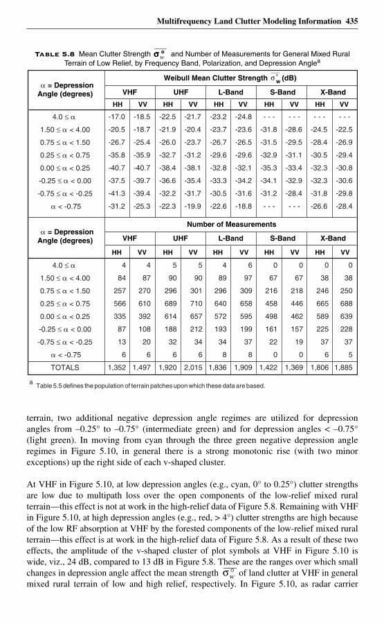
Multifrequency Land Clutter Modeling Information 435

terrain, two additional negative depression angle regimes are utilized for depressionangles from –0.25° to –0.75° (intermediate green) and for depression angles < –0.75°(light green). In moving from cyan through the three green negative depression angleregimes in Figure 5.10, in general there is a strong monotonic rise (with two minorexceptions) up the right side of each v-shaped cluster.

At VHF in Figure 5.10, at low depression angles (e.g., cyan, 0° to 0.25°) clutter strengthsare low due to multipath loss over the open components of the low-relief mixed ruralterrain—this effect is not at work in the high-relief data of Figure 5.8. Remaining with VHFin Figure 5.10, at high depression angles (e.g., red, > 4°) clutter strengths are high becauseof the low RF absorption at VHF by the forested components of the low-relief mixed ruralterrain—this effect is at work in the high-relief data of Figure 5.8. As a result of these twoeffects, the amplitude of the v-shaped cluster of plot symbols at VHF in Figure 5.10 iswide, viz., 24 dB, compared to 13 dB in Figure 5.8. These are the ranges over which smallchanges in depression angle affect the mean strength of land clutter at VHF in generalmixed rural terrain of low and high relief, respectively. In Figure 5.10, as radar carrier

Table 5.8 Mean Clutter Strength and Number of Measurements for General Mixed Rural Terrain of Low Relief, by Frequency Band, Polarization, and Depression Anglea

σ °σ °σ °σ °w

a Table 5.5 defines the population of terrain patches upon which these data are based.

Weibull Mean Clutter Strength w (dB)σ°

HH VV HH VV HH VV HH VV HH VV

HH VV HH VV HH VV HH VV

� = DepressionAngle (degrees)

Number of Measurements � = DepressionAngle (degrees)

UHFVHF L-Band S-Band X-Band

HH VV

UHFVHF L-Band S-Band X-Band

4.0 ≤ �

1.50 ≤ � < 4.00

0.75 ≤ � < 1.50

0.25 ≤ � < 0.75

0.00 ≤ � < 0.25

-0.25 ≤ � < 0.00

-0.75 ≤ � < -0.25

� < -0.75

-17.0

-20.5

-26.7

-35.8

-40.7

-37.5

-41.3

-31.2

4.0 ≤ �

1.50 ≤ � < 4.00

0.75 ≤ � < 1.50

0.25 ≤ � < 0.75

0.00 ≤ � < 0.25

-0.25 ≤ � < 0.00

-0.75 ≤ � < -0.25

� < -0.75

TOTALS

4

84

257

566

335

87

13

6

1,352

4

87

270

610

392

108

20

6

1,497

5

90

296

689

614

188

32

6

1,920

5

90

301

710

657

212

34

6

2,015

4

89

296

640

572

193

34

8

1,836

6

97

309

658

595

199

37

8

1,909

0

67

216

458

498

161

22

0

1,422

0

67

218

446

462

157

19

0

1,369

0

38

246

665

589

225

37

6

1,806

0

38

250

688

639

228

37

5

1,885

-18.5

-18.7

-25.4

-35.9

-40.7

-39.7

-39.4

-25.3

-22.5

-21.9

-26.0

-32.7

-38.4

-36.6

-32.2

-22.3

-21.7

-20.4

-23.7

-31.2

-38.1

-35.4

-31.7

-19.9

-23.2

-23.7

-26.7

-29.6

-32.8

-33.3

-30.5

-22.6

-24.8

-23.6

-26.5

-29.6

-32.1

-34.2

-31.6

-18.8

- - -

-31.8

-31.5

-32.9

-35.3

-34.1

-31.2

- - -

- - -

-28.6

-29.5

-31.1

-33.4

-32.9

-28.4

- - -

- - -

-24.5

-28.4

-30.5

-32.3

-32.3

-31.8

-26.6

- - -

-22.5

-26.9

-29.4

-30.8

-30.6

-29.8

-28.4

σ °w

436 Multifrequency Land Clutter Modeling Information

frequency f rises from VHF into the microwave regime, at low depression angle (cyan) rises from VHF to L-band due to decreasing multipath loss with approximate

dependence ∝ f 0.95, whereas at high depression angle (red and magenta) falls from VHF to S-band due to increasing RF absorption by tree foliage with approximatedependence ∝ f -0.97. At intermediate depression angles, the variation with radarfrequency is intermediate between these extremes. As a result of these two opposite trendswith radar frequency, the data points plotted in Figure 5.10 take on a funnel shape. As in thehigh-relief data of Figure 5.8, there is an S-band dip between L-band and X-band in thelow-relief data of Figure 5.10, with the dip more pronounced at high depression angle(magenta) than at low depression angle (cyan). This dip occurs at all positive depressionangles in Figure 5.10. As in Figure 5.8 at high relief, in Figure 5.10 at low relief thedifferences with polarization are generally small, on the order of several dB or less, withvertical polarization (VV) almost always stronger than horizontal (HH).

Comparison of Figures 5.8 and 5.10 indicates that there exist considerable differences inmean clutter strength between general mixed rural terrain of high relief (terrain slopes> 2°) and low relief (terrain slopes < 2°), respectively. A major reason for this is that low-relief mixed rural terrain allows multipath propagation to occur, which drives down clutterstrengths at low depression angle in the lower bands. Multipath propagation does not occurto any significant degree in high-relief terrain or at high depression angles in low-reliefterrain. At high depression angles in the lower bands and at all depression angles in theupper bands, mean clutter strengths in high-relief terrain are somewhat greater than in low-relief terrain, within similar depression angle regimes. Such differences are due directly tothe effect of terrain relief on intrinsic σ°; they are less than the low depression angledifferences in the lower bands caused by multipath. A contributing factor to all thedifferences in mean clutter strength with terrain relief indicated in Figures 5.8 and 5.10 isthat high-relief mixed rural terrain tends to be somewhat more forested whereas low-reliefmixed rural terrain tends to be somewhat more open. Classification by terrain relief in twomajor regimes as shown in Figures 5.8 and 5.10 is a simple and practicable approach forsorting out the complex phenomenological influences at work in low-angle land clutter.

Table 5.9 presents the Weibull shape parameter aw and ratios of standard deviation-to-meanand mean-to-median for clutter amplitude distributions in general mixed rural terrain oflow relief, by depression angle and radar spatial resolution. The statistical populationsunderlying the data of Table 5.9 are available in Table 5.5. In Table 5.9, aw is calculated twoways: (1) from the ratio of standard deviation-to-mean and (2) from the mean-to-medianratio. Many of the corresponding aw numbers resulting from these two methods ofcalculation are remarkably close in Table 5.9. Each pair of aw numbers in Table 5.9 comesfrom a scatter plot in which each individual point plotted shows the median value of spreadvs the median value of spatial resolution in a group of like-classified measured clutterhistograms. The standard deviation-to-mean scatter plot for the 0.25° to 0.75° depressionangle regime in Table 5.9 is shown in Figure 5.11. The major parametric variation of aw inTable 5.9 is with radar spatial resolution. In every case, aw is much greater at 103 m2

resolution than at 106 m2 resolution. There is a weak trend in Table 5.9 whereby awdecreases as depression angle increases from the 0° to 0.25° regime. There is littleindication for aw in terrain of high relief as shown in Table 5.7 to be lower than in terrain oflow relief as shown in Table 5.9, as might be expected in these results. The lower subtableof Table 5.9 shows the ratios of standard deviation-to-mean and mean-to-median fromwhich the aw numbers in the upper subtable come. The large spreads in low-angle land

σ °w f( )σ °w f( ) σ °w f( )

σ °w f( )

σ °w

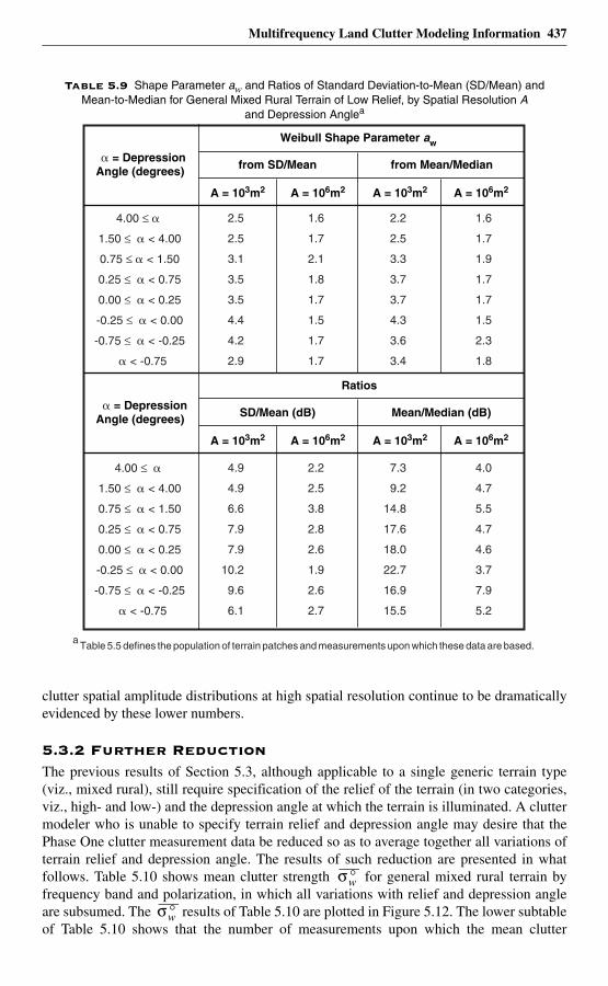
Multifrequency Land Clutter Modeling Information 437

clutter spatial amplitude distributions at high spatial resolution continue to be dramaticallyevidenced by these lower numbers.

5.3.2 Further Reduction The previous results of Section 5.3, although applicable to a single generic terrain type(viz., mixed rural), still require specification of the relief of the terrain (in two categories,viz., high- and low-) and the depression angle at which the terrain is illuminated. A cluttermodeler who is unable to specify terrain relief and depression angle may desire that thePhase One clutter measurement data be reduced so as to average together all variations ofterrain relief and depression angle. The results of such reduction are presented in whatfollows. Table 5.10 shows mean clutter strength for general mixed rural terrain byfrequency band and polarization, in which all variations with relief and depression angleare subsumed. The results of Table 5.10 are plotted in Figure 5.12. The lower subtableof Table 5.10 shows that the number of measurements upon which the mean clutter

Table 5.9 Shape Parameter aw and Ratios of Standard Deviation-to-Mean (SD/Mean) and Mean-to-Median for General Mixed Rural Terrain of Low Relief, by Spatial Resolution A

and Depression Anglea

a Table 5.5 defines the population of terrain patches and measurements upon which these data are based.

Weibull Shape Parameter aw

A = 103m2

� = DepressionAngle (degrees) from SD/Mean from Mean/Median

4.00 ≤ �

1.50 ≤ � < 4.00

0.75 ≤ � < 1.50

0.25 ≤ � < 0.75

0.00 ≤ � < 0.25

-0.25 ≤ � < 0.00

-0.75 ≤ � < -0.25

� < -0.75

2.5

2.5

3.1

3.5

3.5

4.4

4.2

2.9

A = 106m2

1.6

1.7

2.1

1.8

1.7

1.5

1.7

1.7

A = 103m2

2.2

2.5

3.3

3.7

3.7

4.3

3.6

3.4

A = 106m2

Ratios

A = 103m2

� = DepressionAngle (degrees) SD/Mean (dB) Mean/Median (dB)

A = 106m2 A = 103m2 A = 106m2

1.6

1.7

1.9

1.7

1.7

1.5

2.3

1.8

4.00 ≤ �

1.50 ≤ � < 4.00

0.75 ≤ � < 1.50

0.25 ≤ � < 0.75

0.00 ≤ � < 0.25

-0.25 ≤ � < 0.00

-0.75 ≤ � < -0.25

� < -0.75

4.9

4.9

6.6

7.9

7.9

10.2

9.6

6.1

2.2

2.5

3.8

2.8

2.6

1.9

2.6

2.7

7.3

9.2

14.8

17.6

18.0

22.7

16.9

15.5

4.0

4.7

5.5

4.7

4.6

3.7

7.9

5.2

σ °w

σ °w

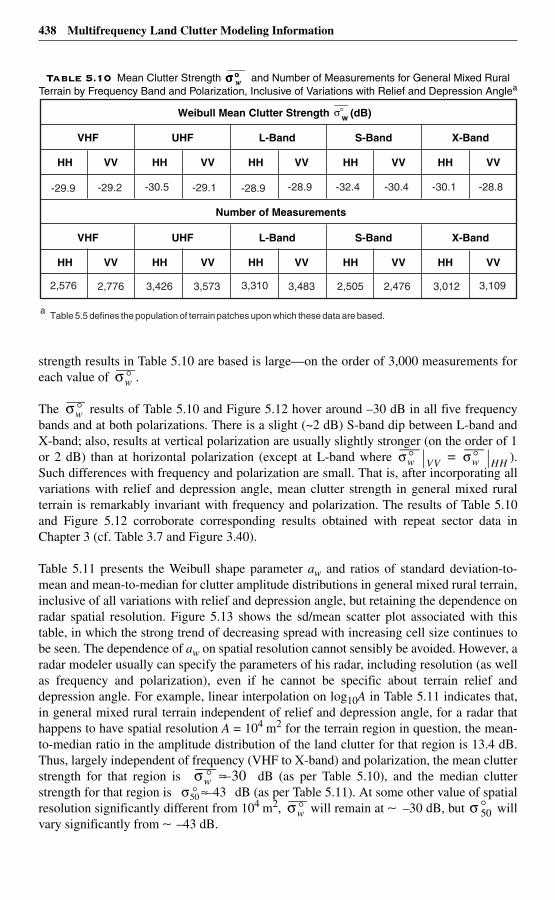
438 Multifrequency Land Clutter Modeling Information

strength results in Table 5.10 are based is large—on the order of 3,000 measurements foreach value of .

The results of Table 5.10 and Figure 5.12 hover around –30 dB in all five frequencybands and at both polarizations. There is a slight (~2 dB) S-band dip between L-band andX-band; also, results at vertical polarization are usually slightly stronger (on the order of 1or 2 dB) than at horizontal polarization (except at L-band where ).Such differences with frequency and polarization are small. That is, after incorporating allvariations with relief and depression angle, mean clutter strength in general mixed ruralterrain is remarkably invariant with frequency and polarization. The results of Table 5.10and Figure 5.12 corroborate corresponding results obtained with repeat sector data inChapter 3 (cf. Table 3.7 and Figure 3.40).

Table 5.11 presents the Weibull shape parameter aw and ratios of standard deviation-to-mean and mean-to-median for clutter amplitude distributions in general mixed rural terrain,inclusive of all variations with relief and depression angle, but retaining the dependence onradar spatial resolution. Figure 5.13 shows the sd/mean scatter plot associated with thistable, in which the strong trend of decreasing spread with increasing cell size continues tobe seen. The dependence of aw on spatial resolution cannot sensibly be avoided. However, aradar modeler usually can specify the parameters of his radar, including resolution (as wellas frequency and polarization), even if he cannot be specific about terrain relief anddepression angle. For example, linear interpolation on log10A in Table 5.11 indicates that,in general mixed rural terrain independent of relief and depression angle, for a radar thathappens to have spatial resolution A = 104 m2 for the terrain region in question, the mean-to-median ratio in the amplitude distribution of the land clutter for that region is 13.4 dB.Thus, largely independent of frequency (VHF to X-band) and polarization, the mean clutterstrength for that region is dB (as per Table 5.10), and the median clutterstrength for that region is dB (as per Table 5.11). At some other value of spatialresolution significantly different from 104 m2, will remain at ∼ –30 dB, but willvary significantly from ∼ –43 dB.

Table 5.10 Mean Clutter Strength and Number of Measurements for General Mixed Rural Terrain by Frequency Band and Polarization, Inclusive of Variations with Relief and Depression Anglea

σ °σ °σ °σ °w

a Table 5.5 defines the population of terrain patches upon which these data are based.

Weibull Mean Clutter Strength w (dB)σ°

HH VV HH VVHH VV HH VV HH VV

L-BandUHF

Number of Measurements

VHF S-Band X-Band

-28.9 -28.9 -32.4 -30.4 -29.9 -29.2 -30.5 -29.1 -30.1 -28.8

HH VV HH VVHH VV HH VV HH VV

L-BandUHFVHF S-Band X-Band

3,310 3,483 2,505 2,4762,576 2,776 3,426 3,573 3,012 3,109

σ °w

σ °w

σ °w VV σ °w HH=

σ °w 30–≈σ50° 43–≈

σ °w σ 50°

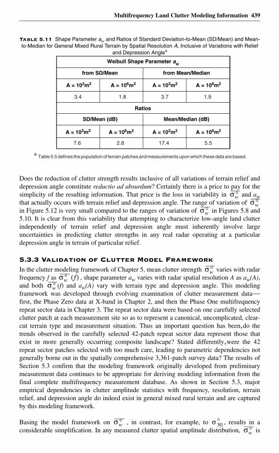
Multifrequency Land Clutter Modeling Information 439

Does the reduction of clutter strength results inclusive of all variations of terrain relief anddepression angle constitute reductio ad absurdum? Certainly there is a price to pay for thesimplicity of the resulting information. That price is the loss in variability in and awthat actually occurs with terrain relief and depression angle. The range of variation of in Figure 5.12 is very small compared to the ranges of variation of in Figures 5.8 and5.10. It is clear from this variability that attempting to characterize low-angle land clutterindependently of terrain relief and depression angle must inherently involve largeuncertainties in predicting clutter strengths in any real radar operating at a particulardepression angle in terrain of particular relief.

5.3.3 Validation of Clutter Model Framework In the clutter modeling framework of Chapter 5, mean clutter strength varies with radarfrequency f as , shape parameter aw varies with radar spatial resolution A as aw(A),and both (f) and aw(A) vary with terrain type and depression angle. This modelingframework was developed through evolving examination of clutter measurement data—first, the Phase Zero data at X-band in Chapter 2, and then the Phase One multifrequencyrepeat sector data in Chapter 3. The repeat sector data were based on one carefully selectedclutter patch at each measurement site so as to represent a canonical, uncomplicated, clear-cut terrain type and measurement situation. Thus an important question has been,do thetrends observed in the carefully selected 42-patch repeat sector data represent those thatexist in more generally occurring composite landscape? Stated differently,were the 42repeat sector patches selected with too much care, leading to parametric dependencies notgenerally borne out in the spatially comprehensive 3,361-patch survey data? The results ofSection 5.3 confirm that the modeling framework originally developed from preliminarymeasurement data continues to be appropriate for deriving modeling information from thefinal complete multifrequency measurement database. As shown in Section 5.3, majorempirical dependencies in clutter amplitude statistics with frequency, resolution, terrainrelief, and depression angle do indeed exist in general mixed rural terrain and are capturedby this modeling framework.

Basing the model framework on , in contrast, for example, to , results in aconsiderable simplification. In any measured clutter spatial amplitude distribution, is

Table 5.11 Shape Parameter aw and Ratios of Standard Deviation-to-Mean (SD/Mean) and Mean-to-Median for General Mixed Rural Terrain by Spatial Resolution A, Inclusive of Variations with Relief

and Depression Anglea

a Table 5.5 defines the population of terrain patches and measurements upon which these data are based.

Weibull Shape Parameter aw

A = 103m2

from SD/Mean from Mean/Median

3.4

A = 106m2

1.8

A = 103m2

3.7

A = 106m2

1.9

Ratios

A = 103m2

SD/Mean (dB) Mean/Median (dB)

7.6

A = 106m2

2.8

A = 103m2

17.4

A = 106m2

5.5

σ °wσ °w

σ °w

σ °wσ °w f( )

σ °w

σ °w σ 50°

σ °w

440 Multifrequency Land Clutter Modeling Information

the only attribute of the distribution not dependent on A. Thus basing the model frameworkon removes one complete parameter dimension from the model—that is, =

(f), whereas = (f, A).

5.3.4 Simplified Clutter Prediction Digitized terrain elevation data27 may often be more readily available to radarperformance modelers than digitized data descriptive of the land cover. For example,although raw Landsat data descriptive of land cover are readily available by purchase fromthe USGS EROS Data Center, these raw data require considerable further processing, firstfor geometric correction, and then for classification into standard land cover categories(e.g., forest, agricultural, etc.), before they are useful for clutter modeling. The cluttermodeling information of Section 5.3, applicable to the single general land cover class of“general mixed rural,” may be directly used for site-specific clutter prediction using onlydigitized terrain elevation data—information descriptive of the land cover at the site is notnecessary in this simplified approach to clutter modeling.

Through use of the digitized terrain elevation data, (1) depression angle from the radar to thebackscattering terrain point can be calculated based simply on the relative elevationdifferences of the radar and the terrain point, and (2) terrain relief can be estimated as high orlow based on whether average terrain slope in the neighborhood of the terrain point is > 2° or< 2°, respectively. This information, together with specification of the radar parameters, issufficient to calculate a Weibull random variate estimate of general mixed rural clutterstrength σ°F4 for the terrain cell in question from the results of Section 5.3.

Of course the disadvantage of this simplified approach is the loss in prediction fidelityassociated with the variations in clutter amplitude statistics that occur with changes in landcover. That such variability can be large is indicated by the clutter modeling informationpresented in Section 5.4 for a number of specifically different land cover classes.However, simplification to the single “general mixed rural” land cover class (i.e., doingwithout land cover information) while retaining variations with relief and depression angleis obviously less severe than further simplifying out variations with relief and depressionangle (i.e., in addition, doing without digitized terrain elevation data) as in the results ofTables 5.10 and 5.11, and Figures 5.12 and 5.13.

5.4 Land Clutter Coefficients for Specific Terrain TypesIn Section 5.4, land clutter coefficients are presented for the following eight specificterrain types—urban, agricultural, forest, shrubland, grassland, wetland, desert, andmountains. These eight terrain types are characterized principally by land cover, except formountain terrain which is characterized principally by landform. The results of Section 5.4are based on the set of 1,733 clutter patches for which the terrain classification is pure.Pure terrain classification implies that a single primary classifier was sufficient to describethe patch; secondary classification was unnecessary. This set of 1,733 pure patches is a

27. Digitized terrain elevation data may be acquired from the U. S. Geological Survey (USGS) or the U. S. National Imagery and Mapping Agency (NIMA). Such data are called Digital Elevation Models (DEMs) by USGS, and Digital Terrain Elevation Data (DTED) by NIMA. In the past, the data from both sources were commonly available at 3 arc-seconds (i.e., ≈100 m) sampling interval, but data at smaller sampling intervals (e.g., 1 arc-second) are now increasingly available.

σ °w σ °wσ °w σ 50

° σ 50°

6Windblown Clutter

Spectral Measurements

6.1 IntroductionMoving target indication (MTI) radar utilizes Doppler processing to separate smallmoving targets from large clutter returns. Any intrinsic motion of the clutter sourcescauses the clutter returns to fluctuate with time and the received clutter power to spreadfrom zero-Doppler in the frequency domain. As a result, intrinsic clutter motion degradesand limits MTI performance. MTI design objectives can require clutter rejection in the 60-to 80-dB range or more, and can be implemented not only by using conventional fixed-parameter MTI filter design [1, 2] but also through modern adaptive Doppler-processingtechniques [3–5]. However implemented, successful clutter rejection to such low levelsrequires accurate definition of the detailed shape of the intrinsic-motion clutter powerspectrum. The most pervasive source of intrinsic fluctuation in ground clutter is the wind-induced motion of tree foliage and branches or other vegetative land cover. The shape ofwindblown tree clutter power spectra has been a subject of investigation since the earlydays of radar development. Although this subject continues to be important, it hasgenerally remained rather poorly understood, largely because of the difficulty ofaccurately measuring clutter spectra to very low spectral power levels.

Radar ground clutter power spectra were originally thought to be of Gaussian shape [6–9].Later, with measurement radars of increased spectral sensitivity, it became apparent thatspectral tails wider than Gaussian existed that could be modeled as power law over thespectral ranges of power—typically 35 to 40 dB below the peak zero-Doppler level—thenavailable [10, 11]. A number of measurements of clutter spectra all generally characterizedas power law followed [12–20], and much discussion at the time focused on power-lawrepresentation of clutter spectral shape. If real when extrapolated to low levels, power-lawspectral tails would severely limit MTI Doppler-processor performance against smalltargets and would reduce motivation for suppressing radar phase noise to lower levels.Measurements of windblown ground clutter power spectra at Lincoln Laboratory to levelssubstantially lower (i.e., 60 to 80 dB down) than most earlier measurements indicatespectral shapes that fall off much more rapidly than constant power-law at rates of decayoften approaching exponential [21–26]. How are these observations of exponential spectralshape reconcilable with the earlier power-law observations? One purpose of Chapter 6 is toresolve these apparently conflicting results.

The most salient aspect of Lincoln Laboratory’s measurements of windblown ground clutterpower spectra is their rapid decay to levels 60 to 80 dB down from zero Doppler. Chapter 6

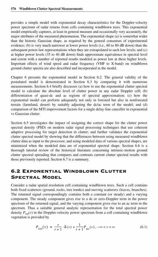
576 Windblown Clutter Spectral Measurements

provides a simple model with exponential decay characteristics for the Doppler-velocitypower spectrum of radar returns from cells containing windblown trees. This exponentialmodel empirically captures, at least in general measure and occasionally very accurately, themajor attributes of the measured phenomenon. The exponential shape (a) is somewhat widerthan the historic Gaussian shape, as required by the general consensus of experimentalevidence; (b) is very much narrower at lower power levels (i.e., 60 to 80 dB down) than thesubsequent power-law representations when they are extrapolated to such low levels; and (c)at higher power levels (35 to 40 dB down) finds approximate equivalence in spectral leveland extent with a number of reported results modeled as power law at these higher levels.Important effects of wind speed and radar frequency (VHF to X-band) on windblownground clutter spectra are also described and incorporated in the model.

Chapter 6 presents the exponential model in Section 6.2. The general validity of thepostulated model is demonstrated in Section 6.3 by comparing it with numerousmeasurements. Section 6.4 briefly discusses (a) how to use the exponential clutter spectralmodel to calculate the absolute level of clutter power in any radar Doppler cell; (b)differentiation of quasi-dc and ac regions of spectral approximation; (c) how theexponential model can perform adequately not only in forested but also in nonforestedterrain (farmland, desert) by suitably adjusting the dc/ac term of the model; and (d)comparison of the MTI improvement factors for a single delay-line canceller in exponentialvs Gaussian clutter.

Section 6.5 investigates the impact of assigning the correct shape for the clutter powerspectral density (PSD) on modern radar signal processing techniques that use coherentadaptive processing for target detection in clutter; and further validates the exponentialclutter spectral model by showing that the differences between using measured windblownclutter data as input to the processor, and using modeled data of various spectral shapes, areminimized when the modeled data are of exponential spectral shape. Section 6.6 is athorough tutorial review of the historical literature concerning intrinsic-motion groundclutter spectral spreading that compares and contrasts current clutter spectral results withthose previously reported. Section 6.7 is a summary.

6.2 Exponential Windblown Clutter Spectral ModelConsider a radar spatial resolution cell containing windblown trees. Such a cell containsboth fixed scatterers (ground, rocks, tree trunks) and moving scatterers (leaves, branches).The returned signal correspondingly contains both a constant (or steady) and a varyingcomponent. The steady component gives rise to a dc or zero-Doppler term in the powerspectrum of the returned signal, and the varying component gives rise to an ac term in thespectrum. Thus a suitable general analytic representation for the total spectral powerdensity Ptot(v) in the Doppler-velocity power spectrum from a cell containing windblownvegetation is provided by

, (6.1)Ptot v( ) rr 1+----------- δ v( ) 1

r 1+-----------Pac v( )+⋅= ∞ v ∞< <–

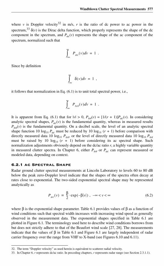
Windblown Clutter Spectral Measurements 577

where v is Doppler velocity32 in m/s, r is the ratio of dc power to ac power in the

spectrum,33 δ(v) is the Dirac delta function, which properly represents the shape of the dccomponent in the spectrum, and Pac(v) represents the shape of the ac component of thespectrum, normalized such that

.

Since by definition

,

it follows that normalization in Eq. (6.1) is to unit total spectral power, i.e.,

.

It is apparent from Eq. (6.1) that for |v| > 0, Ptot(v) = [1/(r + 1)]Pac(v). In consideringanalytic spectral shapes, Pac(v) is the fundamental quantity, whereas in measured resultsPtot(v) is the fundamental quantity. On a decibel scale, the level of an analytic spectralshape function 10 log1 0 Pac must be reduced by 10 log1 0 (r + 1) before comparison withdirectly measured data 10 log1 0 Ptot, or the level of directly measured data 10 log1 0 Ptotmust be raised by 10 log1 0 (r + 1) before considering its ac spectral shape. Suchnormalization adjustments obviously depend on the dc/ac ratio r, a highly variable quantityin measured clutter spectra. In Chapter 6, either Ptot or Pac can represent measured ormodeled data, depending on context.

6.2.1 ac Spectral ShapeRadar ground clutter spectral measurements at Lincoln Laboratory to levels 60 to 80 dBbelow the peak zero-Doppler level indicate that the shapes of the spectra often decay atrates close to exponential. The two-sided exponential spectral shape may be representedanalytically as

, (6.2)

where β is the exponential shape parameter. Table 6.1 provides values of β as a function ofwind conditions such that spectral width increases with increasing wind speed as generallyobserved in the measurement data. The exponential shapes specified in Table 6.1 areplotted in Figure 6.1. The terminology used here to describe wind conditions borrows frombut does not strictly adhere to that of the Beaufort wind scale [27, 28]. The measurementsindicate that the values of β in Table 6.1 and Figure 6.1 are largely independent of radarcarrier frequency over the range from VHF to X-band (see Figures 6.10 and 6.11).

32. The term “Doppler velocity” as used herein is equivalent to scatterer radial velocity.33. In Chapter 6, r represents dc/ac ratio. In preceding chapters, r represents radar range (see Section 2.3.1.1).

Pac v( ) vd∞–

∞

∫ 1=

δ v( ) vd∞–

∞

∫ 1=

Ptot v( ) vd∞–

∞

∫ 1=

Pac v( ) β2--- β v–( )exp⋅= ∞ v ∞< <–

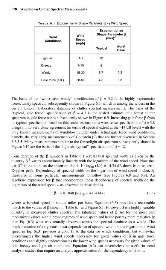
578 Windblown Clutter Spectral Measurements

The basis of the “worst-case, windy” specification of β = 5.2 is the highly exponentialforest/windy spectrum subsequently shown in Figure 6.5, which is among the widest in thecurrent Lincoln Laboratory database of clutter spectral measurements. The basis of the“typical, gale force” specification of β = 4.3 is the scaled estimate of a forest clutterspectrum in gale force winds subsequently shown in Figure 6.9. Increasing gale force β fromits typical specification based on this scaled estimate to a worst-case specification of β = 3.8brings it into very close agreement (in terms of spectral extent at the –14-dB level) with theonly known measurements of windblown clutter under actual gale force wind conditions,namely, the very early measurements of Goldstein [9] that are further discussed in Section6.6.3.5. Many measurements similar to the forest/light air spectrum subsequently shown inFigure 6.16 are the basis of the “light air, typical” specification of β = 12.

Consideration of the β numbers in Table 6.1 reveals that spectral width as given by thequantity β-1 varies approximately linearly with the logarithm of the wind speed. Note thatv = β-1 is the point on the spectrum that is 10 log10 (1/e) = –4.34 dB down from its zero-Doppler peak. Dependency of spectral width on the logarithm of wind speed is directlyillustrated in some particular measurements to follow (see Figures 6.8 and 6.9). Analgebraic expression for β that incorporates linear dependency of spectral width on thelogarithm of the wind speed w as observed in these data is

β-1 = 0.1048 [log10 w + 0.4147] (6.3)

where w is wind speed in statute miles per hour. Equation (6.3) provides a reasonablematch to the values of β shown in Table 6.1 and Figure 6.1. However, β is a highly variablequantity in measured clutter spectra. The tabulated values of β are for the most partmedianized values within broad regimes of wind speed and hence portray more realisticallythan Eq. (6.3) what was actually observed across the spectral database as a whole. Theimplementation of a rigorous linear dependence of spectral width on the logarithm of windspeed in Eq. (6.3) provides a good fit to the data for windy conditions, but somewhatoverestimates the higher wind speeds necessary for given values of β in gale forceconditions and slightly underestimates the lower wind speeds necessary for given values ofβ in breezy and light air conditions. Equation (6.3) can nevertheless be useful in trendanalysis studies that require an analytic approximation for the dependency of β on w.

Table 6.1 Exponential ac Shape Parameter β vs Wind Speed

Exponential acShape Parameter β

(m/s)-1WindConditions

WindSpeed(mph)

TypicalWorstCase

Light air

Breezy

Windy

Gale force (est.)

1-7

7-15

15-30

30-60

12

8

5.7

4.3

—

—

5.2

3.8

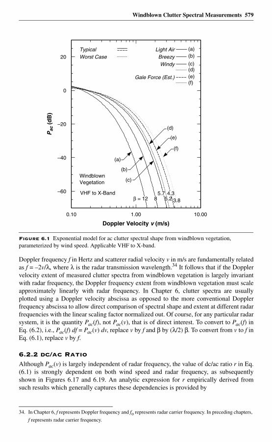
Windblown Clutter Spectral Measurements 579

Doppler frequency f in Hertz and scatterer radial velocity v in m/s are fundamentally relatedas f = –2v/λ, where λ is the radar transmission wavelength.34 It follows that if the Dopplervelocity extent of measured clutter spectra from windblown vegetation is largely invariantwith radar frequency, the Doppler frequency extent from windblown vegetation must scaleapproximately linearly with radar frequency. In Chapter 6, clutter spectra are usuallyplotted using a Doppler velocity abscissa as opposed to the more conventional Dopplerfrequency abscissa to allow direct comparison of spectral shape and extent at different radarfrequencies with the linear scaling factor normalized out. Of course, for any particular radarsystem, it is the quantity Pac(f), not Pac(v), that is of direct interest. To convert to Pac(f) inEq. (6.2), i.e., Pac(f) df = Pac(v) dv, replace v by f and β by (λ/2) β. To convert from v to f inEq. (6.1), replace v by f.

6.2.2 dc/ac RatioAlthough Pac(v) is largely independent of radar frequency, the value of dc/ac ratio r in Eq.(6.1) is strongly dependent on both wind speed and radar frequency, as subsequentlyshown in Figures 6.17 and 6.19. An analytic expression for r empirically derived fromsuch results which generally captures these dependencies is provided by

Figure 6.1 Exponential model for ac clutter spectral shape from windblown vegetation, parameterized by wind speed. Applicable VHF to X-band.

34. In Chapter 6, f represents Doppler frequency and fo represents radar carrier frequency. In preceding chapters,

f represents radar carrier frequency.

20

0

–20

–40

–60

0.10 1.00 10.00

Doppler Velocity v (m/s)

Pac

(d

B)

Windy

Light AirBreezy

Gale Force (Est.)

TypicalWorst Case

β = 85.7

5.24.3

3.812

WindblownVegetation

(a)(b)

(c)(d)(e)(f)

(a)

(b)

(c)

(d)

(e)

(f)

VHF to X-Band

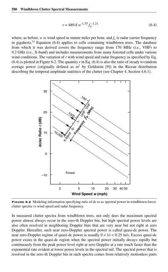
580 Windblown Clutter Spectral Measurements

r = 489.8 w-1.55 fo-1.21 (6.4)

where, as before, w is wind speed in statute miles per hour, and fo is radar carrier frequencyin gigahertz.3 4 Equation (6.4) applies to cells containing windblown trees. The databasefrom which it was derived covers the frequency range from 170 MHz (i.e., VHF) to9.2 GHz (i.e., X-band) and includes measurements from many forested cells under variouswind conditions. The variation of r with wind speed and radar frequency as specified by Eq.(6.4) is plotted in Figure 6.2. The quantity r in Eq. (6.4) is also the ratio of steady to randomaverage power (originally defined as m2 by Goldstein [9]) in the Ricean distributiondescribing the temporal amplitude statistics of the clutter (see Chapter 4, Section 4.6.1).

In measured clutter spectra from windblown trees, not only does the maximum spectralpower almost always occur in the zero-th Doppler bin, but high spectral power levels arealso often resolved in neighboring Doppler bins that are very near but not right at zeroDoppler. Hereafter, such near zero-Doppler spectral power is called quasi-dc power. Thenear zero-Doppler regime of quasi-dc power is usually 0 < |v| < 0.25 m/s. Excess quasi-dcpower exists in the quasi-dc region when the spectral power initially decays rapidly butcontinuously from the peak power level right at zero Doppler at a rate much faster than theexponential rate evident at lower power levels in the spectral tail. The spectral power that isresolved in the zero-th Doppler bin in such spectra comes from relatively motionless parts

Figure 6.2 Modeling information specifying ratio of dc to ac spectral power in windblown forest clutter spectra vs wind speed and radar frequency.

X-Ba

ndS-

L-U

HF

VHF

Freq

uenc

y o

(MH

z)

2 5 10 20 30 40 50

Forest

30

20

10

0

–10

dc/

ac R

atio

r (

dB

)

Wind Speed w (mph)

100

1000

10,000

Windblown Clutter Spectral Measurements 581

of the tree trunks near ground level as well as from the ground surface itself, whereas thespectral power resolved as quasi-dc comes from higher parts of tree trunks and major limbsflexing slightly at very slow rates. Including the excess quasi-dc spectral power as part ofthe ac spectral power degrades the goodness-of-fit of the exponential shape function in thespectral tail. That is, in these circumstances even though the value of β in Eq. (6.2) iscorrectly selected to match the relative shape Pac(v) in the spectral tail, the value of r willbe too low, with the result that the absolute level [1/(r + 1)]Pac(v) will be too high.Furthermore, to the extent that windblown clutter statistics are nonstationary, besides beingtoo high, this level can also be dependent on the length of coherent processing interval(CPI) employed.

Therefore, in what follows, where excess (above the approximating exponential) quasi-dcpower occurs in the data, it is included with the Dirac delta function as dc power in themodel. This approach to quantifying dc/ac ratio r has been followed in the processingunderlying the statistics upon which Eq. (6.2) is based (see Section 6.4.2). The majorconsequence of this approach is that the preceding spectral model approximates theexponential spectral tail region correctly, in both relative shape and absolute level, andindependently of the length of CPI employed. Examples of windblown forest clutterspectra containing excess quasi-dc power are presented subsequently, as well as examplesof desert and cropland clutter spectra in which a dc component from the absolutelystationary underlying ground surface (as opposed to the moving vegetation) exists as adiscrete delta function.

6.2.3 Model ScopeEquations (6.1), (6.2), (6.3), and (6.4) constitute a simple but complete empirical modelfor characterizing the complex physical phenomenon of radar ground clutter powerspectra from windblown trees based on extensive measurements. Total backscatteredclutter power is represented including both dc and ac spectral components. The test of anymodel of a physical phenomenon is the degree to which it generally represents thephenomenon while avoiding complicating detail. The important parameters incorporatedin the model of Eqs. (6.1), (6.2), (6.3), and (6.4) are wind speed and radar frequency;others that might be thought to strongly influence clutter spectra from windblown trees,but which appear to be generally subsumed within the ranges of statistical variability overthe relatively large cell sizes utilized in the measurement data, include: (a) the types oftrees involved (species, density, growth stage), (b) season of the year (e.g., leaves on vsleaves off), (c) wind direction, (d) polarization, and (e) angle of illumination.

It is not possible to generalize information for dc/ac spectral power ratio r for all possiblevarieties of vegetated (or partially vegetated) ground clutter cells from which significantproportions of backscattered clutter power come from stationary scattering elements.Subsequently discussed Lincoln Laboratory measurements of clutter spectra in scrubdesert, rangeland, and cropland terrain, although indicating much larger values of dc/acspectral power ratio when compared with forest terrain, also indicate that the residual acspectral shape function Pac(v) is similar to that of forest. Thus the spectral model of Eqs.(6.1), (6.2), and (6.3), although explicitly derived for windblown trees, may be consideredgenerally applicable not only to forested cells but also, at least as a first-orderapproximation, to cells in partially open or open terrain (desert, rangeland, cropland) aslong as the value of r is increased appropriately. However, Eq. (6.4) specifying r wasderived only from forested cells, and only some particular examples are provided in what

582 Windblown Clutter Spectral Measurements

follows indicating how r increases for cells incompletely filled with trees or in openagricultural terrain.

Although the exponential spectral shapes Pac(v) in Figure 6.1 are modeled to be invariantwith radar frequency and vegetation type, two important ramifications are: (1) modeledwidths of clutter frequency spectra Pac(f) increase linearly with radar frequency from VHFto X-band, and (2) increasing values of dc to ac ratio r in increasingly open terrain (desert,cropland) and/or with decreasing radar frequency cause absolute ac power levels [1/(r+1)]Pac(v) to decrease even though the Pac(v) shape function itself remains invariant under suchcircumstances.

An important requirement in the development of the current model was that its predictionsof spectral extent be in the correct general Doppler regime at spectral power levels 60 to80 dB down from zero-Doppler peaks. Much uncertainty has existed concerning thelocation of this regime. The extensive Lincoln Laboratory database of windblown clutterspectral measurements, without exception, indicates ever increasing rates of spectral decay(i.e., downward curvature) with decreasing spectral power level as observed on log-Dopplervelocity axes such that maximum spectral extents 60 to 80 dB down are limited to Dopplervelocities of 3 to 4 m/s. The exponential shape function properly reflects this importantfundamental feature of the measurements. The exponential model for Pac(v) provideswindblown clutter spectra wider than Gaussian as required by experiment and supported bytheory [29].

An alternative popular spectral shape function Pac(v) has been power-law [10]. Themeasurement data clearly indicate that observed rates of decay modeled as power law atupper levels of spectral power do not continue as power law to lower levels of spectralpower but fall off much faster at the lower levels. In contrast, an exponential representationgenerally captures, at least approximately and occasionally highly accurately, the majorattributes of the windblown clutter ac spectral shape function over the entire range fromnear the zero-Doppler peak to measured levels 60 to 80 dB down.

The exponential model for Pac(v) is validated in Section 6.5 (see also [30, 31]) by showingthat the differences in matched filter and clutter cancellation system performance betweenusing actual measured in-phase (I) and quadrature (Q) Phase One clutter data as input to theprocessors, and modeled clutter spectral data of various spectral shapes (viz., Gaussian,power law, and exponential), are minimized when the spectral model employed is ofexponential shape. Section 6.5 also evaluates the impact of using the exponential model forPac(v), as opposed to Gaussian and power-law models, on the prediction of detectionperformance of airborne and ground-based surveillance radar using coherent adaptiveprocessing [32, 33].

6.3 Measurement Basis for Clutter Spectral Model

6.3.1 Radar Instrumentation and Data ReductionLincoln Laboratory has measured and characterized ground clutter power spectra overwide spectral dynamic ranges using the Phase One and LCE (L-Band Clutter Experiment)instrumentation radars [21, 25]. Both of these radars were conventional analog coherent

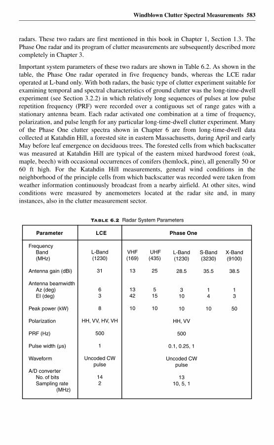
Windblown Clutter Spectral Measurements 583

radars. These two radars are first mentioned in this book in Chapter 1, Section 1.3. ThePhase One radar and its program of clutter measurements are subsequently described morecompletely in Chapter 3.

Important system parameters of these two radars are shown in Table 6.2. As shown in thetable, the Phase One radar operated in five frequency bands, whereas the LCE radaroperated at L-band only. With both radars, the basic type of clutter experiment suitable forexamining temporal and spectral characteristics of ground clutter was the long-time-dwellexperiment (see Section 3.2.2) in which relatively long sequences of pulses at low pulserepetition frequency (PRF) were recorded over a contiguous set of range gates with astationary antenna beam. Each radar activated one combination at a time of frequency,polarization, and pulse length for any particular long-time-dwell clutter experiment. Manyof the Phase One clutter spectra shown in Chapter 6 are from long-time-dwell datacollected at Katahdin Hill, a forested site in eastern Massachusetts, during April and earlyMay before leaf emergence on deciduous trees. The forested cells from which backscatterwas measured at Katahdin Hill are typical of the eastern mixed hardwood forest (oak,maple, beech) with occasional occurrences of conifers (hemlock, pine), all generally 50 or60 ft high. For the Katahdin Hill measurements, general wind conditions in theneighborhood of the principle cells from which backscatter was recorded were taken fromweather information continuously broadcast from a nearby airfield. At other sites, windconditions were measured by anemometers located at the radar site and, in manyinstances, also in the clutter measurement sector.

Table 6.2 Radar System Parameters

Parameter LCE Phase One

Frequency Band (MHz)

Antenna gain (dBi)

Antenna beamwidth Az (deg) EI (deg)

Peak power (kW)

Polarization

PRF (Hz)

Pulse width (µs)

Waveform

A/D converter No. of bits Sampling rate (MHz)

L-Band(1230)

31

63

8

HH, VV, HV, VH

500

1

Uncoded CWpulse

142

VHF(169)

13

1342

10

UHF(435)

25

515

10

L-Band(1230)

28.5

310

10

HH, VV

500

0.1, 0.25, 1

Uncoded CWpulse

1310, 5, 1

S-Band(3230)

35.5

14

10

X-Band(9100)

38.5

13

50

584 Windblown Clutter Spectral Measurements

The LCE radar was a major upgrade at L-band only of the Phase One measurementequipment with substantially reduced phase noise levels [34, 35]. A primary designobjective of the LCE radar was to achieve low enough phase noise such that the low-frequency Doppler components of windblown clutter could be measured to levels ≈ 80 dBbelow the dc or stationary component of the clutter at zero-Doppler. This objective was metby using a combination of low phase-noise local oscillators (viz., Hewlett-Packard models8662A and 8663A) locked to a common source, a low phase-noise transmitter, and systemclocks with low jitter. The transmitter used two planar triodes (viz., Eimac Y-793F) in agrounded-grid amplifier configuration providing inherently low noise sensitivity [36]. TheLCE radar receiver achieved high dynamic range through careful gain distribution andproper choice of mixers and amplifiers, with particular attention paid to maintaining overallsystem linearity. The two channels of the analog in-phase and quadrature (I/Q) detector,which operated at a receiver IF of 3 GHz, were balanced to within approximately 0.1 dB inamplitude and 1 degree of phase. This balance provided approximately 40 dB of imagerejection. The receiver baseband I/Q outputs were digitized by 14-bit analog-to-digital (A/D) converters chosen for their linearity and speed (i.e., maximum clock speed = 10 MHz).The I/Q detector dc bias was temperature-regulated to approximately 100 µV variation (i.e.,to less than the least-significant bit of the A/D converter).

Many of the LCE clutter spectra shown in Chapter 6 are from long-time-dwell datacollected at Wachusett Mountain, Massachusetts, 32 miles west of Katahdin Hill, withsimilar tree cover. A photograph of the LCE radar on Wachusett Mountain is shown inFigure 6.3. Another LCE measurement site was in Nevada, where backscatter data wererecorded from sparse scrub vegetation typical of the western desert. In contrast with PhaseOne, the LCE radar could measure both the copolarized and the cross-polarized returns,although not simultaneously. For LCE clutter measurements at Wachusett Mountain, windconditions were measured simultaneously with the clutter measurements at 10-s updateintervals with an anemometer stationed on top of a 75-ft tower in a treed clutter cell alongone of the three azimuth positions selected for clutter measurements. These measurementswere performed in August with the deciduous trees fully in leaf.

6.3.1.1 Spectral Processing

LCE long-time-dwell clutter data were acquired with a stationary antenna over 70-s datarecording intervals called experiments. Each LCE experiment involved the recording of 80I and Q sample pairs per pulse repetition interval (PRI) at 2- MHz sampling frequency(i.e., 75-m range gate spacing), leading to a 6-km total recorded range swath. Clutterexperiments were usually taken in sequential groups covering the various LCEpolarization combinations. Phase One long-time-dwell clutter data were acquiredsimilarly to LCE data. Table 6.3 provides the specific Phase One clutter data acquisitionand spectral processing parameters applicable to the Phase One spectral results shownherein from Katahdin Hill.

All the LCE clutter power spectra shown subsequently were computed directly as fastFourier transforms (FFTs) of the sampled temporal pulse-by-pulse return, including the dccomponent. A four-term Blackman-Harris window function was utilized, with highestsidelobe level at –92 dB [37]. Each temporal record of 30,720 pulses (first 61.44 s of each70-s experiment) was divided into contiguous groups of 5,120 samples; a 1,024-pointcomplex FFT was generated for each group by utilizing every fifth pulse; and theamplitudes of the resultant set of FFTs were arithmetically averaged together in each

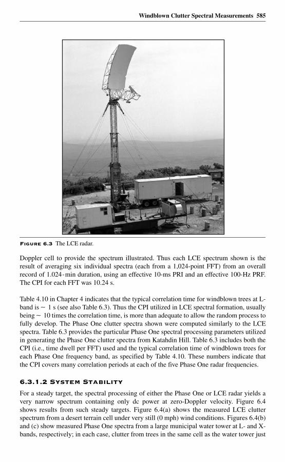
Windblown Clutter Spectral Measurements 585

Doppler cell to provide the spectrum illustrated. Thus each LCE spectrum shown is theresult of averaging six individual spectra (each from a 1,024-point FFT) from an overallrecord of 1.024-min duration, using an effective 10-ms PRI and an effective 100-Hz PRF.The CPI for each FFT was 10.24 s.

Table 4.10 in Chapter 4 indicates that the typical correlation time for windblown trees at L-band is ∼ 1 s (see also Table 6.3). Thus the CPI utilized in LCE spectral formation, usuallybeing ∼ 10 times the correlation time, is more than adequate to allow the random process tofully develop. The Phase One clutter spectra shown were computed similarly to the LCEspectra. Table 6.3 provides the particular Phase One spectral processing parameters utilizedin generating the Phase One clutter spectra from Katahdin Hill. Table 6.3 includes both theCPI (i.e., time dwell per FFT) used and the typical correlation time of windblown trees foreach Phase One frequency band, as specified by Table 4.10. These numbers indicate thatthe CPI covers many correlation periods at each of the five Phase One radar frequencies.

6.3.1.2 System Stability

For a steady target, the spectral processing of either the Phase One or LCE radar yields avery narrow spectrum containing only dc power at zero-Doppler velocity. Figure 6.4shows results from such steady targets. Figure 6.4(a) shows the measured LCE clutterspectrum from a desert terrain cell under very still (0 mph) wind conditions. Figures 6.4(b)and (c) show measured Phase One spectra from a large municipal water tower at L- and X-bands, respectively; in each case, clutter from trees in the same cell as the water tower just

Figure 6.3 The LCE radar.

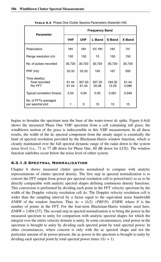
586 Windblown Clutter Spectral Measurements

begins to broaden the spectrum near the base of the water-tower dc spike. Figure 6.4(d)shows the measured Phase One VHF spectrum from a cell containing tall grass; thewindblown motion of the grass is indiscernible in this VHF measurement. In all theseresults, the width of the dc spectral component from the steady target is essentially thelimit of spectral resolution provided by the Blackman-Harris window function, which iscleanly maintained over the full spectral dynamic range of the radar down to the systemnoise level (i.e., 71 to 77 dB down for Phase One, 80 dB down for LCE). The windowfunction sidelobes occur below the noise level of either system.

6.3.1.3 Spectral Normalization

Chapter 6 shows measured clutter spectra normalized to compare with analyticrepresentations of clutter spectral density. The first step in spectral normalization is toconvert the FFT output from power per spectral resolution cell to power/(m/s) so as to bedirectly comparable with analytic spectral shapes defining continuous density functions.This conversion is performed by dividing each point in the FFT velocity spectrum by thewidth of the Doppler velocity resolution cell ∆v. The Doppler velocity resolution cell iswider than the sampling interval by a factor equal to the equivalent noise bandwidthENBW of the window function. Thus ∆v = (λ/2) ⋅(PRF/N) ⋅ENBW, where N is thenumber of points in the FFT. For the four-term Blackman-Harris window used here,ENBW = 2.004 [37]. The second step in spectral normalization is to bring the power in themeasured spectrum to unity for comparison with analytic spectral shapes for which theintegral over the entire velocity domain is unity. In some circumstances, total power in thespectrum is brought to unity by dividing each spectral point by total spectral power. Inother circumstances, where concern is only with the ac spectral shape and not theparticular amount of dc power present, the ac power in the spectrum is brought to unity bydividing each spectral point by total spectral power times 1/(r + 1).

Table 6.3 Phase One Clutter Spectra Parameters (Katahdin Hill)

Frequency Band Parameter

VHF UHF L-Band S-Band X-Band

Polarization

Range resolution (m)

No. of pulses recorded

PRF (Hz)

Time dwell(s) Total recorded Per FFT

Typical correlation time(s)

No. of FFTs averagedper spectral plot

HH

150

30,720

33.33

61.4461.44

5.04

1

HH

150

30,720

33.33

307.2061.44

0.94

5

VV, HH

15

30,720

100

307.2020.48

0.95

15

HH

150

30,720

167

184.3212.29

0.081

15

VV

150

30,720

500

61.444.096

0.049

15

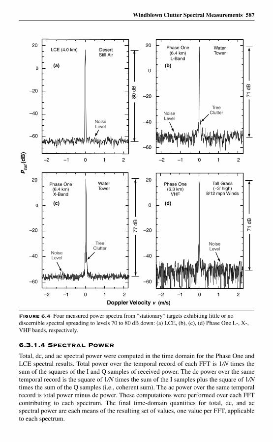
Windblown Clutter Spectral Measurements 587

6.3.1.4 Spectral Power

Total, dc, and ac spectral power were computed in the time domain for the Phase One andLCE spectral results. Total power over the temporal record of each FFT is 1/N times thesum of the squares of the I and Q samples of received power. The dc power over the sametemporal record is the square of 1/N times the sum of the I samples plus the square of 1/Ntimes the sum of the Q samples (i.e., coherent sum). The ac power over the same temporalrecord is total power minus dc power. These computations were performed over each FFTcontributing to each spectrum. The final time-domain quantities for total, dc, and acspectral power are each means of the resulting set of values, one value per FFT, applicableto each spectrum.

Figure 6.4 Four measured power spectra from “stationary” targets exhibiting little or no discernible spectral spreading to levels 70 to 80 dB down: (a) LCE, (b), (c), (d) Phase One L-, X-, VHF bands, respectively.

–2 0 2

71

dB

WaterTower

–1 1–2 0 2

–60

–40

–20

0

20

80

dB

LCE (4.0 km) DesertStill Air

–1 1

71

dB

–2 0 2

–60

–40

–20

0

20

Doppler Velocity v (m/s)

–1 1

NoiseLevel

NoiseLevel

NoiseLevel

Tall Grass(~3' high)

8/12 mph Winds

77

dB

–2 0 2–1 1

–60

–40

–20

0

20WaterTower

Phase One(6.4 km)X-Band

(a) (b)

(c) (d)

Pto

t (d

B)

TreeClutter

TreeClutter

NoiseLevel

–60

–40

–20

0

20

Phase One(6.3 km)

VHF

Phase One(6.4 km)L-Band

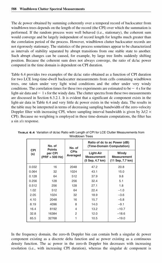
588 Windblown Clutter Spectral Measurements

The dc power obtained by summing coherently over a temporal record of backscatter fromwindblown trees depends on the length of the record (the CPI) over which the summation isperformed. If the random process were well behaved (i.e., stationary), the coherent sumwould converge and be largely independent of record length for lengths much greater thanthe correlation period of the process. However, windblown clutter backscatter records arenot rigorously stationary. The statistics of the process sometimes appear to be characterizedas intervals of stability separated by abrupt transitions from one stable state to another.Such abrupt changes can be caused, for example, by large tree limbs suddenly shiftingposition. Because the coherent sum does not always converge, the ratio of dc/ac powercomputed in the time domain is dependent on CPI duration.

Table 6.4 provides two examples of the dc/ac ratio obtained as a function of CPI durationfor two LCE long-time-dwell backscatter measurements from cells containing windblowntrees, one taken under very light wind conditions and the other under very windyconditions. The correlation times for these two experiments are estimated to be ∼ 4 s for thelight-air data and ∼ 1 s for the windy data. The clutter spectra from these two measurementsare discussed in Section 6.3.2.1. It is evident that a significant dc component exists in thelight-air data in Table 6.4 and very little dc power exists in the windy data. The results inthe table may be interpreted in terms of decreasing sampling bandwidth of the zero-velocityDoppler filter with increasing CPI, where sampling interval bandwidth is given by λ/(2 ×CPI). Because no weighting is employed in these time-domain computations, the filter hasa sin x/x response.

In the frequency domain, the zero-th Doppler bin can contain both a singular dc powercomponent existing as a discrete delta function and ac power existing as a continuousdensity function. The ac power in the zero-th Doppler bin decreases with increasingresolution (i.e., with increasing CPI duration), whereas the singular dc component is

Table 6.4 Variation of dc/ac Ratio with Length of CPI for LCE Clutter Measurements from Windblown Trees

CPI(s)

No. ofPointsper CPI

(PRF = 500 Hz)

No. ofCPIs

Averaged

Ratio of dc to ac Power (dB)(Time-Domain Computation)

Light-AirMeasurement

(5 Sep, 4.7 km)

WindyMeasurement

(11 Sep, 7.7 km)

0.032

0.064

0.128

0.256

0.512

1.02

2.05

4.10

8.19

16.4

32.8

65.5

16

32

64

128

256

512

1024

2048

4096

8192

16384

32768

2048

1024

512

256

128

64

32

16

8

4

2

1

47.2

43.1

37.9

32.4

27.1

22.4

18.9

15.7

14.0

13.2

12.0

10.5

20.8

15.0

9.8

5.1

1.8

–1.0

–3.6

–5.8

–9.1

–10.7

–18.6

–19.0

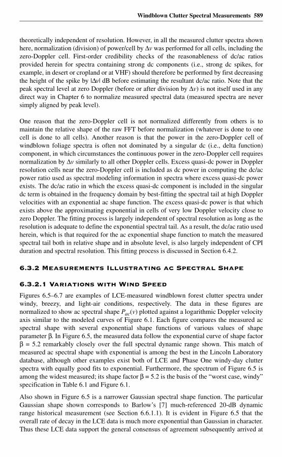
Windblown Clutter Spectral Measurements 589

theoretically independent of resolution. However, in all the measured clutter spectra shownhere, normalization (division) of power/cell by ∆v was performed for all cells, including thezero-Doppler cell. First-order credibility checks of the reasonableness of dc/ac ratiosprovided herein for spectra containing strong dc components (i.e., strong dc spikes, forexample, in desert or cropland or at VHF) should therefore be performed by first decreasingthe height of the spike by |∆v| dB before estimating the resultant dc/ac ratio. Note that thepeak spectral level at zero Doppler (before or after division by ∆v) is not itself used in anydirect way in Chapter 6 to normalize measured spectral data (measured spectra are neversimply aligned by peak level).

One reason that the zero-Doppler cell is not normalized differently from others is tomaintain the relative shape of the raw FFT before normalization (whatever is done to onecell is done to all cells). Another reason is that the power in the zero-Doppler cell ofwindblown foliage spectra is often not dominated by a singular dc (i.e., delta function)component, in which circumstances the continuous power in the zero-Doppler cell requiresnormalization by ∆v similarly to all other Doppler cells. Excess quasi-dc power in Dopplerresolution cells near the zero-Doppler cell is included as dc power in computing the dc/acpower ratio used as spectral modeling information in spectra where excess quasi-dc powerexists. The dc/ac ratio in which the excess quasi-dc component is included in the singulardc term is obtained in the frequency domain by best-fitting the spectral tail at high Dopplervelocities with an exponential ac shape function. The excess quasi-dc power is that whichexists above the approximating exponential in cells of very low Doppler velocity close tozero Doppler. The fitting process is largely independent of spectral resolution as long as theresolution is adequate to define the exponential spectral tail. As a result, the dc/ac ratio usedherein, which is that required for the ac exponential shape function to match the measuredspectral tail both in relative shape and in absolute level, is also largely independent of CPIduration and spectral resolution. This fitting process is discussed in Section 6.4.2.

6.3.2 Measurements Illustrating ac Spectral Shape

6.3.2.1 Variations with Wind Speed

Figures 6.5–6.7 are examples of LCE-measured windblown forest clutter spectra underwindy, breezy, and light-air conditions, respectively. The data in these figures arenormalized to show ac spectral shape Pac(v) plotted against a logarithmic Doppler velocityaxis similar to the modeled curves of Figure 6.1. Each figure compares the measured acspectral shape with several exponential shape functions of various values of shapeparameter β. In Figure 6.5, the measured data follow the exponential curve of shape factorβ = 5.2 remarkably closely over the full spectral dynamic range shown. This match ofmeasured ac spectral shape with exponential is among the best in the Lincoln Laboratorydatabase, although other examples exist both of LCE and Phase One windy-day clutterspectra with equally good fits to exponential. Furthermore, the spectrum of Figure 6.5 isamong the widest measured; its shape factor β = 5.2 is the basis of the “worst case, windy”specification in Table 6.1 and Figure 6.1.

Also shown in Figure 6.5 is a narrower Gaussian spectral shape function. The particularGaussian shape shown corresponds to Barlow’s [7] much-referenced 20-dB dynamicrange historical measurement (see Section 6.6.1.1). It is evident in Figure 6.5 that theoverall rate of decay in the LCE data is much more exponential than Gaussian in character.Thus these LCE data support the general consensus of agreement subsequently arrived at

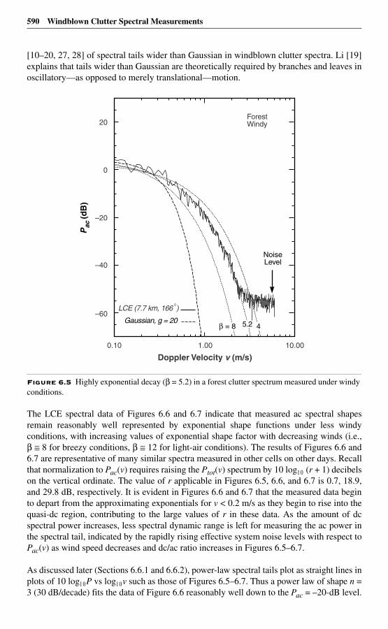
590 Windblown Clutter Spectral Measurements

[10–20, 27, 28] of spectral tails wider than Gaussian in windblown clutter spectra. Li [19]explains that tails wider than Gaussian are theoretically required by branches and leaves inoscillatory—as opposed to merely translational—motion.

The LCE spectral data of Figures 6.6 and 6.7 indicate that measured ac spectral shapesremain reasonably well represented by exponential shape functions under less windyconditions, with increasing values of exponential shape factor with decreasing winds (i.e.,β ≅ 8 for breezy conditions, β ≅ 12 for light-air conditions). The results of Figures 6.6 and6.7 are representative of many similar spectra measured in other cells on other days. Recallthat normalization to Pac(v) requires raising the Ptot(v) spectrum by 10 log1 0 (r + 1) decibelson the vertical ordinate. The value of r applicable in Figures 6.5, 6.6, and 6.7 is 0.7, 18.9,and 29.8 dB, respectively. It is evident in Figures 6.6 and 6.7 that the measured data beginto depart from the approximating exponentials for v < 0.2 m/s as they begin to rise into thequasi-dc region, contributing to the large values of r in these data. As the amount of dcspectral power increases, less spectral dynamic range is left for measuring the ac power inthe spectral tail, indicated by the rapidly rising effective system noise levels with respect toPac(v) as wind speed decreases and dc/ac ratio increases in Figures 6.5–6.7.

As discussed later (Sections 6.6.1 and 6.6.2), power-law spectral tails plot as straight lines inplots of 10 log1 0P vs log1 0v such as those of Figures 6.5–6.7. Thus a power law of shape n =3 (30 dB/decade) fits the data of Figure 6.6 reasonably well down to the Pac = –20-dB level.

Figure 6.5 Highly exponential decay (β = 5.2) in a forest clutter spectrum measured under windy conditions.

1.00 10.00

–60

–40

–20

0

20

Doppler Velocity v (m/s)

Pac

(dB

)

LCE (7.7 km, 166 )

0.10

Gaussian, g = 20

NoiseLevel

ForestWindy

= 8 5.2 4

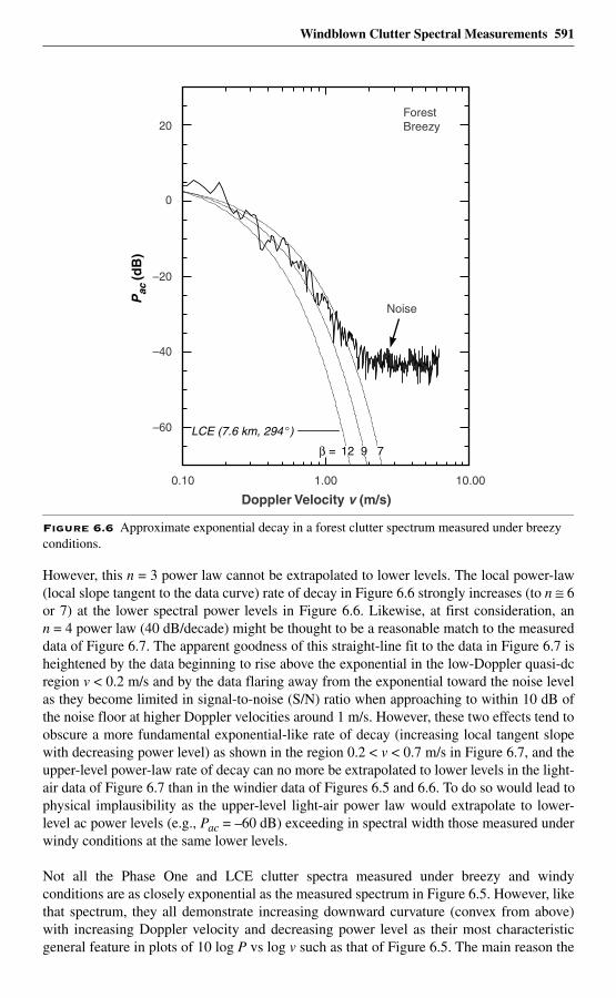
Windblown Clutter Spectral Measurements 591

However, this n = 3 power law cannot be extrapolated to lower levels. The local power-law(local slope tangent to the data curve) rate of decay in Figure 6.6 strongly increases (to n ≅ 6or 7) at the lower spectral power levels in Figure 6.6. Likewise, at first consideration, ann = 4 power law (40 dB/decade) might be thought to be a reasonable match to the measureddata of Figure 6.7. The apparent goodness of this straight-line fit to the data in Figure 6.7 isheightened by the data beginning to rise above the exponential in the low-Doppler quasi-dcregion v < 0.2 m/s and by the data flaring away from the exponential toward the noise levelas they become limited in signal-to-noise (S/N) ratio when approaching to within 10 dB ofthe noise floor at higher Doppler velocities around 1 m/s. However, these two effects tend toobscure a more fundamental exponential-like rate of decay (increasing local tangent slopewith decreasing power level) as shown in the region 0.2 < v < 0.7 m/s in Figure 6.7, and theupper-level power-law rate of decay can no more be extrapolated to lower levels in the light-air data of Figure 6.7 than in the windier data of Figures 6.5 and 6.6. To do so would lead tophysical implausibility as the upper-level light-air power law would extrapolate to lower-level ac power levels (e.g., Pac = –60 dB) exceeding in spectral width those measured underwindy conditions at the same lower levels.

Not all the Phase One and LCE clutter spectra measured under breezy and windyconditions are as closely exponential as the measured spectrum in Figure 6.5. However, likethat spectrum, they all demonstrate increasing downward curvature (convex from above)with increasing Doppler velocity and decreasing power level as their most characteristicgeneral feature in plots of 10 log P vs log v such as that of Figure 6.5. The main reason the

Figure 6.6 Approximate exponential decay in a forest clutter spectrum measured under breezy conditions.

1.00 10.00

–60

–40

–20

0

20

Doppler Velocity v (m/s)

Pac

(dB

)

ForestBreezy

0.10

=

LCE (7.6 km, 294 )

12 9 7

Noise

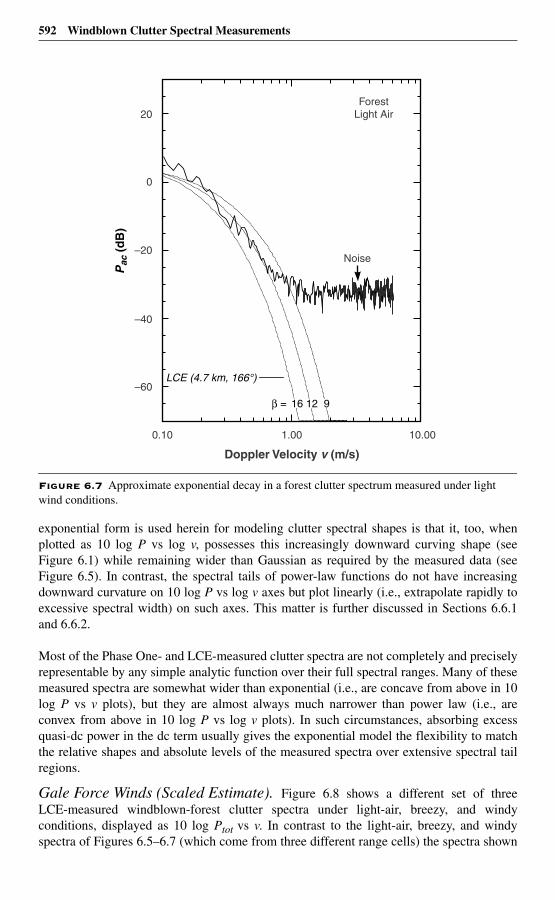
592 Windblown Clutter Spectral Measurements

exponential form is used herein for modeling clutter spectral shapes is that it, too, whenplotted as 10 log P vs log v, possesses this increasingly downward curving shape (seeFigure 6.1) while remaining wider than Gaussian as required by the measured data (seeFigure 6.5). In contrast, the spectral tails of power-law functions do not have increasingdownward curvature on 10 log P vs log v axes but plot linearly (i.e., extrapolate rapidly toexcessive spectral width) on such axes. This matter is further discussed in Sections 6.6.1and 6.6.2.

Most of the Phase One- and LCE-measured clutter spectra are not completely and preciselyrepresentable by any simple analytic function over their full spectral ranges. Many of thesemeasured spectra are somewhat wider than exponential (i.e., are concave from above in 10log P vs v plots), but they are almost always much narrower than power law (i.e., areconvex from above in 10 log P vs log v plots). In such circumstances, absorbing excessquasi-dc power in the dc term usually gives the exponential model the flexibility to matchthe relative shapes and absolute levels of the measured spectra over extensive spectral tailregions.

Gale Force Winds (Scaled Estimate). Figure 6.8 shows a different set of threeLCE-measured windblown-forest clutter spectra under light-air, breezy, and windyconditions, displayed as 10 log Ptot vs v. In contrast to the light-air, breezy, and windyspectra of Figures 6.5–6.7 (which come from three different range cells) the spectra shown

Figure 6.7 Approximate exponential decay in a forest clutter spectrum measured under light wind conditions.

1.00 10.00

–60

–40

–20

0

20

Doppler Velocity v (m/s)

Pac

(d

B)

ForestLight Air

0.10

β =

LCE (4.7 km, 166°)

16 12 9

Noise

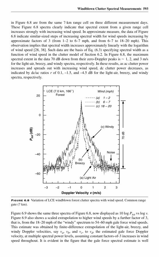
Windblown Clutter Spectral Measurements 593

in Figure 6.8 are from the same 7-km range cell on three different measurement days.These Figure 6.8 spectra clearly indicate that spectral extent from a given range cellincreases strongly with increasing wind speed. In approximate measure, the data of Figure6.8 indicate similar-sized steps of increasing spectral width for wind speeds increasing byapproximate factors of 3 (from 1–2 to 6–7 mph, and from 6–7 to 18–20 mph). Thisobservation implies that spectral width increases approximately linearly with the logarithmof wind speed [28, 38]. Such data are the basis of Eq. (6.3) specifying spectral width as afunction of wind speed in the clutter model of Section 6.2. In Figure 6.8, the maximumspectral extent in the data 70 dB down from their zero-Doppler peaks is ∼ 1, 2, and 3 m/sfor the light-air, breezy, and windy spectra, respectively. In these results, as ac clutter powerincreases and spreads out with increasing wind speed, dc clutter power decreases, asindicated by dc/ac ratios r of 0.1, –1.5, and –4.5 dB for the light-air, breezy, and windyspectra, respectively.

Figure 6.9 shows the same three spectra of Figure 6.8, now displayed as 10 log Ptot vs log v.Figure 6.9 also shows a scaled extrapolation to higher wind speeds by a further factor of 3,that is, from the 18–20 mph of the “windy” spectrum to 54–60 mph gale force wind speeds.This estimate was obtained by finite-difference extrapolation of the light-air, breezy, andwindy Doppler velocities, say va, vb, and vc, to vd, the estimated gale force Dopplervelocity, at multiple spectral power levels, assuming constant factors-of-3 increases in windspeed throughout. It is evident in the figure that the gale force spectral estimate is well

Figure 6.8 Variation of LCE windblown forest clutter spectra with wind speed. Common range gate (7 km).

–2 0 2

Doppler Velocity v (m/s)

–3

–60

–40

–20

0

20

3

70

dB

(a) Light Air

(b)Breezy

(c) Windy

LCE (7.0 km, 166 )Forest

Noise

1–1

(a)(b)(c)

1 – 26 – 7

18 – 20

Wind (mph)

Pto

t (d

B)

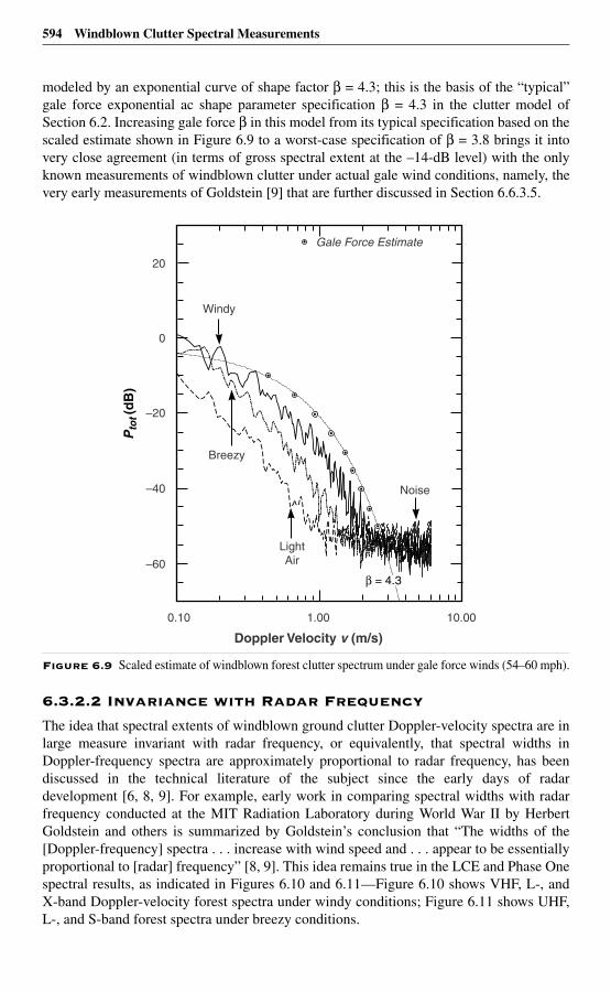
594 Windblown Clutter Spectral Measurements

modeled by an exponential curve of shape factor β = 4.3; this is the basis of the “typical”gale force exponential ac shape parameter specification β = 4.3 in the clutter model ofSection 6.2. Increasing gale force β in this model from its typical specification based on thescaled estimate shown in Figure 6.9 to a worst-case specification of β = 3.8 brings it intovery close agreement (in terms of gross spectral extent at the –14-dB level) with the onlyknown measurements of windblown clutter under actual gale wind conditions, namely, thevery early measurements of Goldstein [9] that are further discussed in Section 6.6.3.5.

6.3.2.2 Invariance with Radar Frequency

The idea that spectral extents of windblown ground clutter Doppler-velocity spectra are inlarge measure invariant with radar frequency, or equivalently, that spectral widths inDoppler-frequency spectra are approximately proportional to radar frequency, has beendiscussed in the technical literature of the subject since the early days of radardevelopment [6, 8, 9]. For example, early work in comparing spectral widths with radarfrequency conducted at the MIT Radiation Laboratory during World War II by HerbertGoldstein and others is summarized by Goldstein’s conclusion that “The widths of the[Doppler-frequency] spectra . . . increase with wind speed and . . . appear to be essentiallyproportional to [radar] frequency” [8, 9]. This idea remains true in the LCE and Phase Onespectral results, as indicated in Figures 6.10 and 6.11—Figure 6.10 shows VHF, L-, andX-band Doppler-velocity forest spectra under windy conditions; Figure 6.11 shows UHF,L-, and S-band forest spectra under breezy conditions.

Figure 6.9 Scaled estimate of windblown forest clutter spectrum under gale force winds (54–60 mph).

1.00 10.00

–60

–40

–20

0

20

Doppler Velocity v (m/s)

Pto

t (d

B)

Gale Force Estimate

0.10

Noise

= 4.3

LightAir

Breezy

Windy

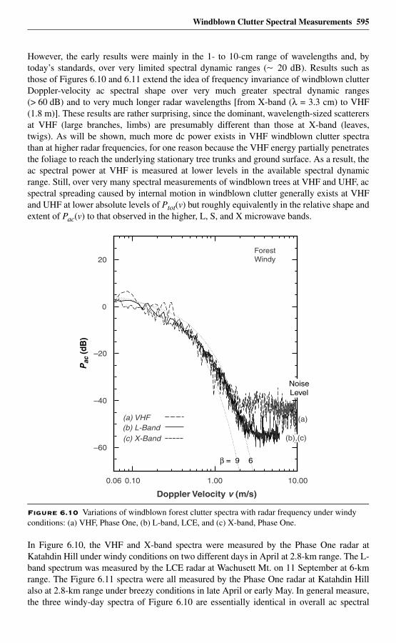
Windblown Clutter Spectral Measurements 595

However, the early results were mainly in the 1- to 10-cm range of wavelengths and, bytoday’s standards, over very limited spectral dynamic ranges (∼ 20 dB). Results such asthose of Figures 6.10 and 6.11 extend the idea of frequency invariance of windblown clutterDoppler-velocity ac spectral shape over very much greater spectral dynamic ranges(> 60 dB) and to very much longer radar wavelengths [from X-band (λ = 3.3 cm) to VHF(1.8 m)]. These results are rather surprising, since the dominant, wavelength-sized scatterersat VHF (large branches, limbs) are presumably different than those at X-band (leaves,twigs). As will be shown, much more dc power exists in VHF windblown clutter spectrathan at higher radar frequencies, for one reason because the VHF energy partially penetratesthe foliage to reach the underlying stationary tree trunks and ground surface. As a result, theac spectral power at VHF is measured at lower levels in the available spectral dynamicrange. Still, over very many spectral measurements of windblown trees at VHF and UHF, acspectral spreading caused by internal motion in windblown clutter generally exists at VHFand UHF at lower absolute levels of Ptot(v) but roughly equivalently in the relative shape andextent of Pac(v) to that observed in the higher, L, S, and X microwave bands.

In Figure 6.10, the VHF and X-band spectra were measured by the Phase One radar atKatahdin Hill under windy conditions on two different days in April at 2.8-km range. The L-band spectrum was measured by the LCE radar at Wachusett Mt. on 11 September at 6-kmrange. The Figure 6.11 spectra were all measured by the Phase One radar at Katahdin Hillalso at 2.8-km range under breezy conditions in late April or early May. In general measure,the three windy-day spectra of Figure 6.10 are essentially identical in overall ac spectral

Figure 6.10 Variations of windblown forest clutter spectra with radar frequency under windy conditions: (a) VHF, Phase One, (b) L-band, LCE, and (c) X-band, Phase One.

0.06 1.00 10.00

–60

–40

–20

0

20

Doppler Velocity v (m/s)

Pac

(dB

)

(c) X-Band

(a) VHF(b) L-Band

ForestWindy

0.10

(a)

NoiseLevel

= 9 6

(b),(c)

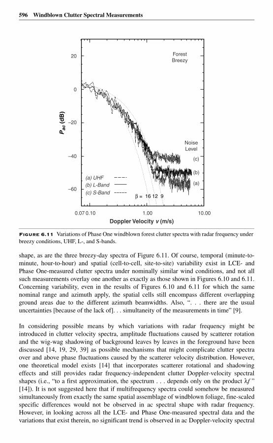
596 Windblown Clutter Spectral Measurements

shape, as are the three breezy-day spectra of Figure 6.11. Of course, temporal (minute-to-minute, hour-to-hour) and spatial (cell-to-cell, site-to-site) variability exist in LCE- andPhase One-measured clutter spectra under nominally similar wind conditions, and not allsuch measurements overlay one another as exactly as those shown in Figures 6.10 and 6.11.Concerning variability, even in the results of Figures 6.10 and 6.11 for which the samenominal range and azimuth apply, the spatial cells still encompass different overlappingground areas due to the different azimuth beamwidths. Also, “. . . there are the usualuncertainties [because of the lack of]. . . simultaneity of the measurements in time” [9].

In considering possible means by which variations with radar frequency might beintroduced in clutter velocity spectra, amplitude fluctuations caused by scatterer rotationand the wig-wag shadowing of background leaves by leaves in the foreground have beendiscussed [14, 19, 29, 39] as possible mechanisms that might complicate clutter spectraover and above phase fluctuations caused by the scatterer velocity distribution. However,one theoretical model exists [14] that incorporates scatterer rotational and shadowingeffects and still provides radar frequency-independent clutter Doppler-velocity spectralshapes (i.e., “to a first approximation, the spectrum . . . depends only on the product λf ”[14]). It is not suggested here that if multifrequency spectra could somehow be measuredsimultaneously from exactly the same spatial assemblage of windblown foliage, fine-scaledspecific differences would not be observed in ac spectral shape with radar frequency.However, in looking across all the LCE- and Phase One-measured spectral data and thevariations that exist therein, no significant trend is observed in ac Doppler-velocity spectral

Figure 6.11 Variations of Phase One windblown forest clutter spectra with radar frequency under breezy conditions, UHF, L-, and S-bands.

0.07 1.00 10.00

–60

–40

–20

0

20

Doppler Velocity v (m/s)

Pac

(d

B)

(c) S-Band

(a) UHF(b) L-Band

ForestBreezy

0.10

NoiseLevel

(a)

(b)

(c)

= 16 12 9

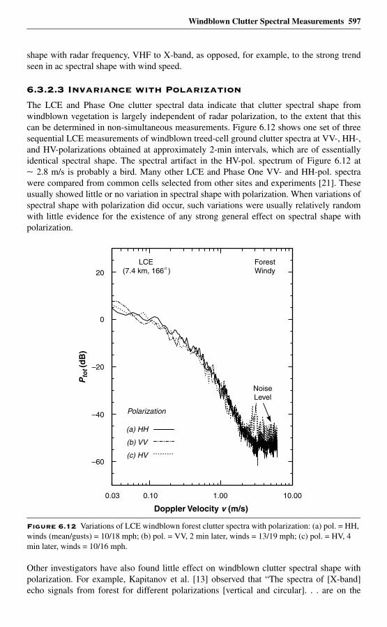
Windblown Clutter Spectral Measurements 597

shape with radar frequency, VHF to X-band, as opposed, for example, to the strong trendseen in ac spectral shape with wind speed.

6.3.2.3 Invariance with Polarization

The LCE and Phase One clutter spectral data indicate that clutter spectral shape fromwindblown vegetation is largely independent of radar polarization, to the extent that thiscan be determined in non-simultaneous measurements. Figure 6.12 shows one set of threesequential LCE measurements of windblown treed-cell ground clutter spectra at VV-, HH-,and HV-polarizations obtained at approximately 2-min intervals, which are of essentiallyidentical spectral shape. The spectral artifact in the HV-pol. spectrum of Figure 6.12 at∼ 2.8 m/s is probably a bird. Many other LCE and Phase One VV- and HH-pol. spectrawere compared from common cells selected from other sites and experiments [21]. Theseusually showed little or no variation in spectral shape with polarization. When variations ofspectral shape with polarization did occur, such variations were usually relatively randomwith little evidence for the existence of any strong general effect on spectral shape withpolarization.

Other investigators have also found little effect on windblown clutter spectral shape withpolarization. For example, Kapitanov et al. [13] observed that “The spectra of [X-band]echo signals from forest for different polarizations [vertical and circular]. . . are on the

Figure 6.12 Variations of LCE windblown forest clutter spectra with polarization: (a) pol. = HH, winds (mean/gusts) = 10/18 mph; (b) pol. = VV, 2 min later, winds = 13/19 mph; (c) pol. = HV, 4 min later, winds = 10/16 mph.

0.03 0.10 1.00 10.00

–60

–40

–20

0

20

Doppler Velocity v (m/s)

Pto

t (d

B)

ForestWindy

LCE(7.4 km, 166 )

(a) HH

(b) VV

(c) HV

Polarization

NoiseLevel

598 Windblown Clutter Spectral Measurements

average similar.” Unpublished X-band windblown clutter spectral results obtained atLincoln Laboratory by Ewell [20] at VV-, HH-, and circular polarizations in shrubby desertterrain also indicated no consistent differences in the spectral shapes obtained at the variouspolarizations.

6.3.2.4 Temporal Variation

All LCE clutter spectra in Chapter 6 are averages of six individual 1,024-point FFTs, eachformed from a 10.24-s duration temporal backscatter record. Windy-day wind conditionsfrequently vary considerably from one 10-s interval to the next. Such variability of windy-day conditions within a treed resolution cell from one 10.24-s interval to the next oftenleads to significant variability in successive individual 10.24-s dwell FFTs [21]. However,the results of Figures 6.13 and 6.14 indicate that over longer periods of 60- to 80-s, windy-day treed-cell clutter spectra can be expected to become more stationary. Figure 6.13shows LCE treed-cell clutter spectra for three repeated experiments on a windy day, eachof which is formed from an overall temporal record of 61.44 s (100-Hz PRF, 1024-pointFFTs, 6 FFTs averaged). The shape of the spectrum from the first experiment is essentiallyidentically replicated by the shape of the spectrum from a following experiment begun 65min later, suggesting that enough averaging of wind variations occurs within 1 min to leadto some degree of convergence in average spectral shape. But wind is an extremely non-stationary dynamic random process with complex short- and long-term variation. Forexample, on the windy/gusty day on which the data of Figure 6.13 were collected, thegusts happened to die down over the 70-s interval covering the second experiment (begun9 min after the first), and the spectrum formed from that data is indeed considerablynarrower than the other two.

Figure 6.14 shows Phase One L-band clutter spectra for three repeated breezy-dayexperiments for very nearly the same treed cell at Wachusett Mt. for which the LCE data ofFigure 6.13 apply. Each of these Phase One spectra is formed from a temporal record of81.9-s duration (125-Hz PRF, 2048-point FFTs, 5 FFTs averaged). The spectrum from thefirst experiment is nearly identical to that of the second experiment, begun 4 min later. Thespectrum from the third experiment, begun 9 min after the first, is somewhat narrower. In asimilar set of five sequential experiments begun 15 min before those of Figure 6.14, therange of variability of spectral shape was similar. The slightly changing average windconditions within 81.9-s intervals over 4- or 5-min periods resulted in only very smallchanges in the measured spectra, such as shown in Figure 6.14. Such results indicate that therange of variability in clutter spectra formed by averaging over 60- to 80-s data intervalsunder nominally similar wind conditions generally is quite low, compared with the morevariable individual FFTs formed from 10- to 16-s data intervals during the same period.

6.3.2.5 Effects of Site/Season/Tree Species/Cell Size

It is not difficult to find Phase One and LCE spectra of essentially identical exponentialspectral shape—two are shown in Figure 6.15. The LCE spectrum (a) measured onSeptember 10 (leaves on deciduous trees) at Wachusett Mt. at 7.9-km range, HH-pol., 150-mrange resolution, and 2° depression angle essentially overlays and replicates the Phase Onespectrum (b) which was measured on May 3 (leaves not yet emerged) at Katahdin Hill at2.4-km range, VV-pol., 15-m range resolution, and 0.5° depression angle. These twomeasurements were obtained with different radar receivers, and the two spectra wereproduced using different data reduction and processing software. Thus commonality can

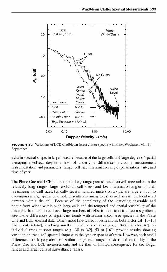
Windblown Clutter Spectral Measurements 599

exist in spectral shape, in large measure because of the large cells and large degree of spatialaveraging involved, despite a host of underlying differences including measurementinstrumentation and parameters (range, cell size, illumination angle, polarization), site, andtime of year.

The Phase One and LCE radars mimic long-range ground-based surveillance radars in therelatively long ranges, large resolution cell sizes, and low illumination angles of theirmeasurements. Cell sizes, typically several hundred meters on a side, are large enough toencompass a large spatial ensemble of scatterers (many trees) as well as variable local windcurrents within the cell. Because of the complexity of the scattering ensemble andnonuniform winds within such large cells and the temporal and spatial variability of theensemble from cell to cell over large numbers of cells, it is difficult to discern significantsite-to-site differences or significant trends with season and/or tree species in the PhaseOne and LCE spectral data. Other, more fine-scaled investigations, both historical [13–16]and recent [40–42], involving small illumination spot sizes (e.g., 1.8-m diameter [42]) onindividual trees at short ranges (e.g., 30 m [42], 50 m [16]), provide results showingvariation on treed-cell spectral shape with the type or species of trees. However, such smalldifferences are largely absorbed within the general ranges of statistical variability in thePhase One and LCE measurements and are thus of limited consequence for the longerranges and larger cells of surveillance radars.

Figure 6.13 Variations of LCE windblown forest clutter spectra with time: Wachusett Mt., 11 September.

0.03 0.10 1.00 10.00

–60

–40

–20

0

20

Doppler Velocity v (m/s)

Pto

t (d

B)

LCE(7.6 km, 166 )

NoiseLevel

ForestWindy/Gusty

Gusts

No Gusts

First

9 min Later

65 min Later

(Exp. Duration = 61.44 s)

Experiment

WindSpeed(mph)Mean/ Gusts

10/18

8/None

13/18

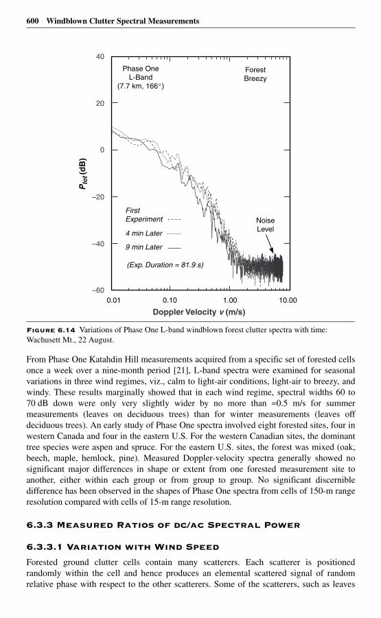
600 Windblown Clutter Spectral Measurements

From Phase One Katahdin Hill measurements acquired from a specific set of forested cellsonce a week over a nine-month period [21], L-band spectra were examined for seasonalvariations in three wind regimes, viz., calm to light-air conditions, light-air to breezy, andwindy. These results marginally showed that in each wind regime, spectral widths 60 to70 dB down were only very slightly wider by no more than ≈0.5 m/s for summermeasurements (leaves on deciduous trees) than for winter measurements (leaves offdeciduous trees). An early study of Phase One spectra involved eight forested sites, four inwestern Canada and four in the eastern U.S. For the western Canadian sites, the dominanttree species were aspen and spruce. For the eastern U.S. sites, the forest was mixed (oak,beech, maple, hemlock, pine). Measured Doppler-velocity spectra generally showed nosignificant major differences in shape or extent from one forested measurement site toanother, either within each group or from group to group. No significant discernibledifference has been observed in the shapes of Phase One spectra from cells of 150-m rangeresolution compared with cells of 15-m range resolution.

6.3.3 Measured Ratios of dc/ac Spectral Power

6.3.3.1 Variation with Wind Speed

Forested ground clutter cells contain many scatterers. Each scatterer is positionedrandomly within the cell and hence produces an elemental scattered signal of randomrelative phase with respect to the other scatterers. Some of the scatterers, such as leaves

Figure 6.14 Variations of Phase One L-band windblown forest clutter spectra with time: Wachusett Mt., 22 August.

–60

–40

–20

0

20

P

tot (d

B)

40

ForestBreezy

0.01 0.10 1.00 10.00

Doppler Velocity v (m/s)

Phase OneL-Band

(7.7 km, 166 )

NoiseLevel

FirstExperiment

4 min Later

9 min Later

(Exp. Duration = 81.9 s)

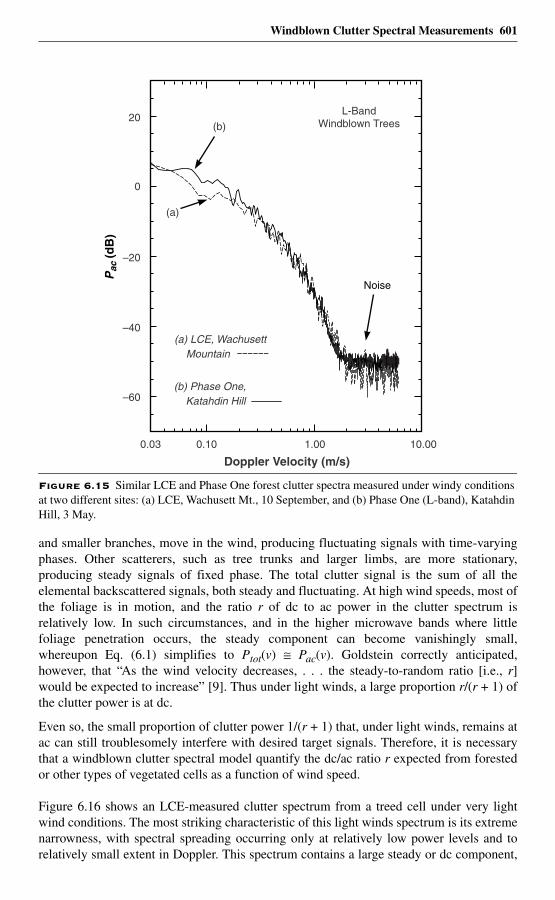
Windblown Clutter Spectral Measurements 601

and smaller branches, move in the wind, producing fluctuating signals with time-varyingphases. Other scatterers, such as tree trunks and larger limbs, are more stationary,producing steady signals of fixed phase. The total clutter signal is the sum of all theelemental backscattered signals, both steady and fluctuating. At high wind speeds, most ofthe foliage is in motion, and the ratio r of dc to ac power in the clutter spectrum isrelatively low. In such circumstances, and in the higher microwave bands where littlefoliage penetration occurs, the steady component can become vanishingly small,whereupon Eq. (6.1) simplifies to Ptot(v) ≅ Pac(v). Goldstein correctly anticipated,however, that “As the wind velocity decreases, . . . the steady-to-random ratio [i.e., r]would be expected to increase” [9]. Thus under light winds, a large proportion r/(r + 1) ofthe clutter power is at dc.

Even so, the small proportion of clutter power 1/(r + 1) that, under light winds, remains atac can still troublesomely interfere with desired target signals. Therefore, it is necessarythat a windblown clutter spectral model quantify the dc/ac ratio r expected from forestedor other types of vegetated cells as a function of wind speed.

Figure 6.16 shows an LCE-measured clutter spectrum from a treed cell under very lightwind conditions. The most striking characteristic of this light winds spectrum is its extremenarrowness, with spectral spreading occurring only at relatively low power levels and torelatively small extent in Doppler. This spectrum contains a large steady or dc component,

Figure 6.15 Similar LCE and Phase One forest clutter spectra measured under windy conditions at two different sites: (a) LCE, Wachusett Mt., 10 September, and (b) Phase One (L-band), Katahdin Hill, 3 May.

0.03 1.00 10.00

–60

–40

–20

0

20

Doppler Velocity (m/s)

Pac

(dB

)

0.10

Noise

(a)

(b)

(b) Phase One, Katahdin Hill

(a) LCE, Wachusett Mountain

L-BandWindblown Trees

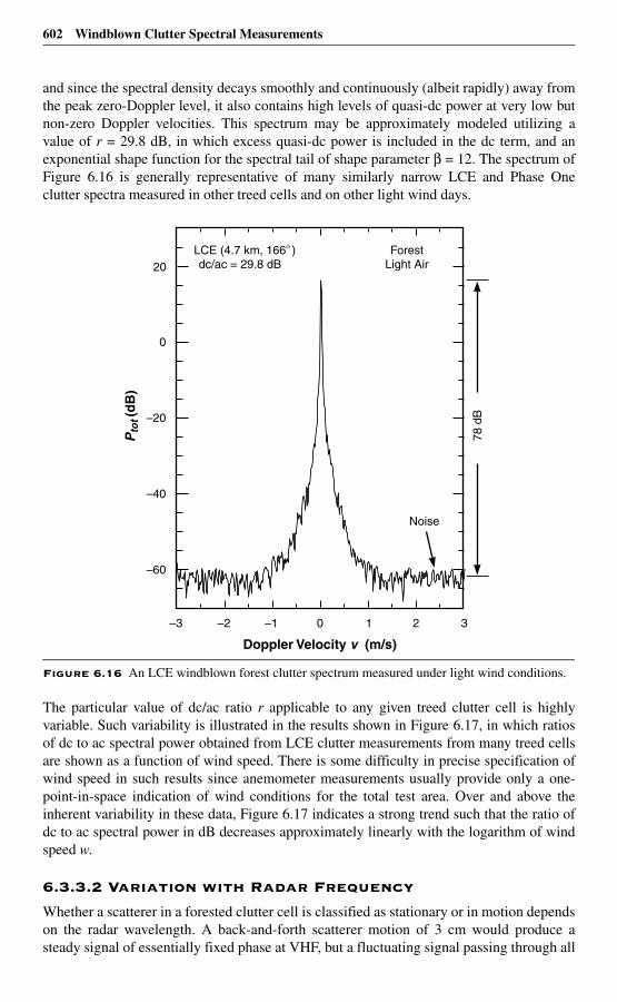
602 Windblown Clutter Spectral Measurements

and since the spectral density decays smoothly and continuously (albeit rapidly) away fromthe peak zero-Doppler level, it also contains high levels of quasi-dc power at very low butnon-zero Doppler velocities. This spectrum may be approximately modeled utilizing avalue of r = 29.8 dB, in which excess quasi-dc power is included in the dc term, and anexponential shape function for the spectral tail of shape parameter β = 12. The spectrum ofFigure 6.16 is generally representative of many similarly narrow LCE and Phase Oneclutter spectra measured in other treed cells and on other light wind days.

The particular value of dc/ac ratio r applicable to any given treed clutter cell is highlyvariable. Such variability is illustrated in the results shown in Figure 6.17, in which ratiosof dc to ac spectral power obtained from LCE clutter measurements from many treed cellsare shown as a function of wind speed. There is some difficulty in precise specification ofwind speed in such results since anemometer measurements usually provide only a one-point-in-space indication of wind conditions for the total test area. Over and above theinherent variability in these data, Figure 6.17 indicates a strong trend such that the ratio ofdc to ac spectral power in dB decreases approximately linearly with the logarithm of windspeed w.

6.3.3.2 Variation with Radar Frequency

Whether a scatterer in a forested clutter cell is classified as stationary or in motion dependson the radar wavelength. A back-and-forth scatterer motion of 3 cm would produce asteady signal of essentially fixed phase at VHF, but a fluctuating signal passing through all

Figure 6.16 An LCE windblown forest clutter spectrum measured under light wind conditions.

–2 0 2

–60

–40

–20

0

20

Doppler Velocity v (m/s)

Pto

t (d

B)

78

dB

3–3

LCE (4.7 km, 166 )dc/ac = 29.8 dB

ForestLight Air

Noise

–1 1

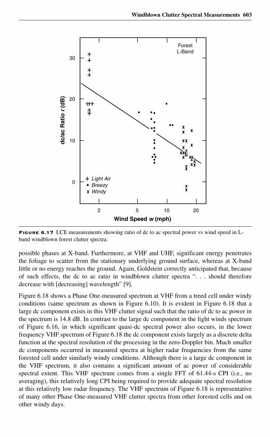
Windblown Clutter Spectral Measurements 603

possible phases at X-band. Furthermore, at VHF and UHF, significant energy penetratesthe foliage to scatter from the stationary underlying ground surface, whereas at X-bandlittle or no energy reaches the ground. Again, Goldstein correctly anticipated that, becauseof such effects, the dc to ac ratio in windblown clutter spectra “. . . should thereforedecrease with [decreasing] wavelength” [9].

Figure 6.18 shows a Phase One-measured spectrum at VHF from a treed cell under windyconditions (same spectrum as shown in Figure 6.10). It is evident in Figure 6.18 that alarge dc component exists in this VHF clutter signal such that the ratio of dc to ac power inthe spectrum is 14.8 dB. In contrast to the large dc component in the light winds spectrumof Figure 6.16, in which significant quasi-dc spectral power also occurs, in the lowerfrequency VHF spectrum of Figure 6.18 the dc component exists largely as a discrete deltafunction at the spectral resolution of the processing in the zero-Doppler bin. Much smallerdc components occurred in measured spectra at higher radar frequencies from the sameforested cell under similarly windy conditions. Although there is a large dc component inthe VHF spectrum, it also contains a significant amount of ac power of considerablespectral extent. This VHF spectrum comes from a single FFT of 61.44-s CPI (i.e., noaveraging), this relatively long CPI being required to provide adequate spectral resolutionat this relatively low radar frequency. The VHF spectrum of Figure 6.18 is representativeof many other Phase One-measured VHF clutter spectra from other forested cells and onother windy days.

Figure 6.17 LCE measurements showing ratio of dc to ac spectral power vs wind speed in L-band windblown forest clutter spectra.

5 10 20

0

10

20

30

Wind Speed w (mph)

dc/

ac R

atio

r (

dB

)

ForestL-Band

Light AirBreezyWindy

2

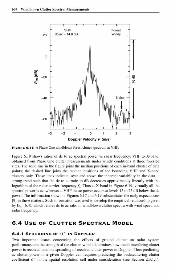
604 Windblown Clutter Spectral Measurements

Figure 6.19 shows ratios of dc to ac spectral power vs radar frequency, VHF to X-band,obtained from Phase One clutter measurements under windy conditions at three forestedsites. The solid line in the figure joins the median positions of each in-band cluster of datapoints; the dashed line joins the median positions of the bounding VHF and X-bandclusters only. These lines indicate, over and above the inherent variability in the data, astrong trend such that the dc to ac ratio in dB decreases approximately linearly with thelogarithm of the radar carrier frequency fo. Thus at X-band in Figure 6.19, virtually all thespectral power is ac, whereas at VHF the ac power occurs at levels 15 to 25 dB below the dcpower. The information shown in Figures 6.17 and 6.19 substantiates the early expectations[9] in these matters. Such information was used to develop the empirical relationship givenby Eq. (6.4), which relates dc to ac ratio in windblown clutter spectra with wind speed andradar frequency.

6.4 Use of Clutter Spectral Model

6.4.1 Spreading of σ ° in DopplerTwo important issues concerning the effects of ground clutter on radar systemperformance are the strength of the clutter, which determines how much interfering clutterpower is received, and the spreading of received clutter power in Doppler. Thus predictingac clutter power in a given Doppler cell requires predicting the backscattering cluttercoefficient σ° in the spatial resolution cell under consideration (see Section 2.3.1.1),

Figure 6.18 A Phase One windblown forest clutter spectrum at VHF.

–2 0 2

–60

–40

–20

0

20

Doppler Velocity v (m/s)

Pto

t (d

B)

76

dB3–3

ForestWindy

VHFdc/ac = 14.8 dB

–1 1

Noise

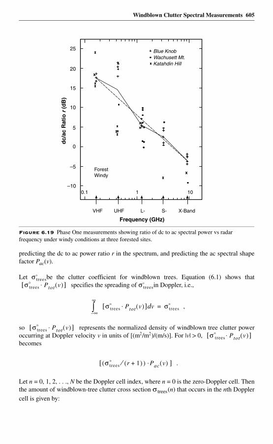
Windblown Clutter Spectral Measurements 605

predicting the dc to ac power ratio r in the spectrum, and predicting the ac spectral shapefactor Pac(v).

Let be the clutter coefficient for windblown trees. Equation (6.1) shows that specifies the spreading of in Doppler, i.e.,

,

so represents the normalized density of windblown tree clutter poweroccurring at Doppler velocity v in units of [(m2/m2)/(m/s)]. For |v| > 0, becomes

.

Let n = 0, 1, 2, . . ., N be the Doppler cell index, where n = 0 is the zero-Doppler cell. Thenthe amount of windblown-tree clutter cross section σ trees(n) that occurs in the nth Dopplercell is given by:

Figure 6.19 Phase One measurements showing ratio of dc to ac spectral power vs radar frequency under windy conditions at three forested sites.

–10

–5

0

5

10

15

20

0.1 1 10

VHF UHF L- S- X-Band

Frequency (GHz)

dc/

ac R

atio

r (

dB

)

Blue KnobWachusett Mt.Katahdin Hill

ForestWindy

25

σ trees°

σ trees° Ptot v( )⋅[ ] σ trees

°

σ trees° Ptot v( )⋅[ ] vd

∞–

∞

∫ σ trees°=

σ trees° Ptot v( )⋅[ ]

σ trees° Ptot v( )⋅[ ]

σ( trees° r 1+( ) )⁄ Pac v( )⋅[ ]

606 Windblown Clutter Spectral Measurements

(6.5)

where σ trees(n) is in units of [m2], and fn is the Doppler frequency [Hz] in the center of thenth Doppler cell. In Eq. (6.5), ∆f = Doppler cell width [Hz]; λ = radar wavelength [m]; A =spatial resolution cell area [m2]; r = ratio of dc/ac spectral power [as given by Eq. (6.4)]; andPac(fn) is the value at f = fn of the ac spectral shape function [as given by Eqs. (6.2) and (6.3)].

Comprehensive information specifying the clutter coefficient in Eq. (6.5) is providedin earlier chapters for the low illumination angles typical of ground-sited radar, for radarfrequencies from VHF to X-band, and for both VV- and HH-polarizations, on the basis ofthe Phase Zero and Phase One clutter measurement databases. These clutter data are notavailable at cross-polarization. However, the LCE clutter data at Wachusett Mt. indicatethat in forest, cross-pol. clutter coefficients are generally 3 to 6 dB but occasionally as littleas 0 dB or as much as 8 dB less than the co-pol. clutter coefficients. Similar depolarizationeffects in forest clutter data have been observed elsewhere [13, 27, 43].

6.4.2 Two Regions of Spectral ApproximationFigure 6.20 shows an idealized representation of a typical windblown clutter spectrum(solid line). As is often observed in measured clutter spectral data, this representationconsists of two distinct regions, namely, a quasi-dc region near zero-Doppler velocity andan ac spectral tail region at greater Doppler velocities. Also shown is a spectral model(dashed lines) as given by Eq. (6.1). The model uses a delta function at v = 0 to representthe dc spectral component and the exponential shape function as given by Eq. (6.2) torepresent the ac spectral tail. In a plot of 10 log10 Ptot vs v such as that of the figure, theexponential shape plots as a straight line of slope 4.34 β (where 4.34 = 10 log10 e and e =2.718 ...). Also, both the data and the model in Figure 6.20 are normalized to unit totalspectral power, i.e.,

.

In these circumstances, the model is matched to the data as follows: first, β is selected sothat the slope [i.e., dB/(m/s)] of the model matches that of the data in the ac spectral tailregion. Next, the value of dc/ac ratio r in the model is assigned to provide a y-intercept [1/(r + 1)](β/2) so that the exponential model overlays and matches the ac region of the datain absolute power level Ptot(v) (i.e., vertical position) as well as slope. Because of thenormalizations involved, this procedure results in the excess power from the quasi-dcregion of the data being included in the dc Dirac delta function term [r/(r + 1)]δ(v) of themodel, where excess quasi-dc power means the power in the quasi-dc region of the datathat exists above the approximating exponential of the model.

Figure 6.21 shows four examples of measured windblown clutter spectra presented as10 log Ptot(v) vs v to illustrate quasi-dc and ac spectral regions in actual measured data.Figure 6.21(a) shows an LCE spectrum; Figures 6.21(b) through (d) show Phase Onespectra at L-, X-, and UHF bands, respectively. Each spectrum has an approximatingexponential model shown as a straight line through the right side of the data. Each spectrumin Figure 6.21 contains excess power above the approximating exponential in a quasi-dc

σtrees n( )σtrees

° λ2 r 1+( )------------------- ∆ f A Pac fn( ) n 0>,⋅⋅⋅=

σ trees°

Ptot v( ) vd∞–

∞

∫ 1=

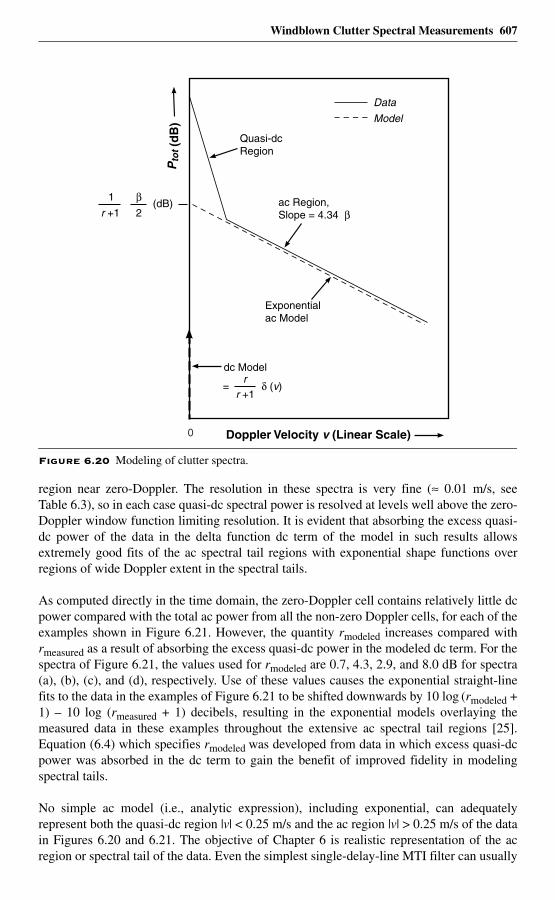
Windblown Clutter Spectral Measurements 607

region near zero-Doppler. The resolution in these spectra is very fine (≈ 0.01 m/s, seeTable 6.3), so in each case quasi-dc spectral power is resolved at levels well above the zero-Doppler window function limiting resolution. It is evident that absorbing the excess quasi-dc power of the data in the delta function dc term of the model in such results allowsextremely good fits of the ac spectral tail regions with exponential shape functions overregions of wide Doppler extent in the spectral tails.

As computed directly in the time domain, the zero-Doppler cell contains relatively little dcpower compared with the total ac power from all the non-zero Doppler cells, for each of theexamples shown in Figure 6.21. However, the quantity rmodeled increases compared withrmeasured as a result of absorbing the excess quasi-dc power in the modeled dc term. For thespectra of Figure 6.21, the values used for rmodeled are 0.7, 4.3, 2.9, and 8.0 dB for spectra(a), (b), (c), and (d), respectively. Use of these values causes the exponential straight-linefits to the data in the examples of Figure 6.21 to be shifted downwards by 10 log (rmodeled +1) – 10 log (rmeasured + 1) decibels, resulting in the exponential models overlaying themeasured data in these examples throughout the extensive ac spectral tail regions [25].Equation (6.4) which specifies rmodeled was developed from data in which excess quasi-dcpower was absorbed in the dc term to gain the benefit of improved fidelity in modelingspectral tails.

No simple ac model (i.e., analytic expression), including exponential, can adequatelyrepresent both the quasi-dc region |v| < 0.25 m/s and the ac region |v| > 0.25 m/s of the datain Figures 6.20 and 6.21. The objective of Chapter 6 is realistic representation of the acregion or spectral tail of the data. Even the simplest single-delay-line MTI filter can usually

Figure 6.20 Modeling of clutter spectra.

Pto

t (d

B)

0

1 βr +1 2

Exponentialac Model

Quasi-dcRegion

ac Region,Slope = 4.34 β

rr +1

δ (v)

dc Model

Data

Model

Doppler Velocity v (Linear Scale)

(dB)

=

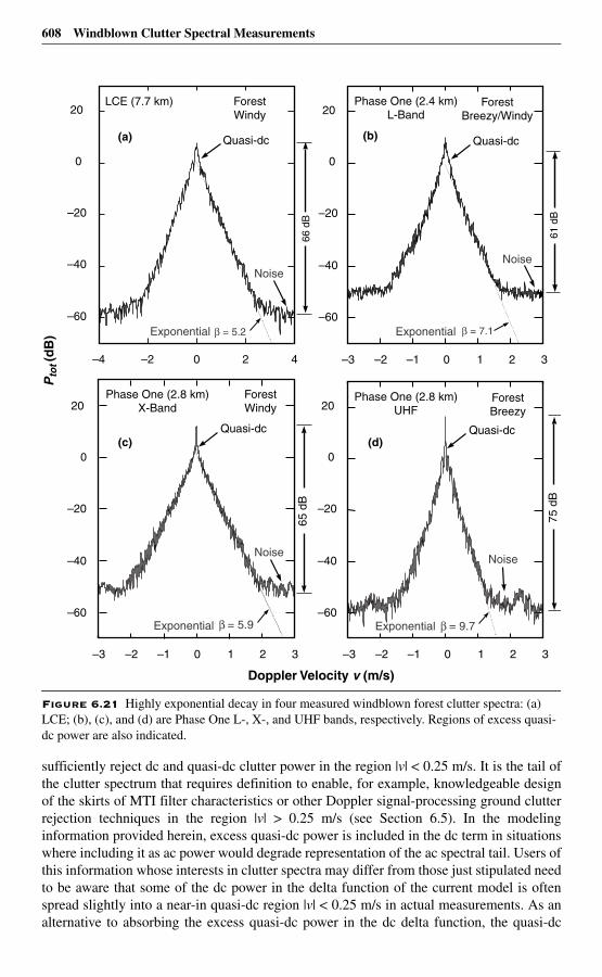
608 Windblown Clutter Spectral Measurements

sufficiently reject dc and quasi-dc clutter power in the region |v| < 0.25 m/s. It is the tail ofthe clutter spectrum that requires definition to enable, for example, knowledgeable designof the skirts of MTI filter characteristics or other Doppler signal-processing ground clutterrejection techniques in the region |v| > 0.25 m/s (see Section 6.5). In the modelinginformation provided herein, excess quasi-dc power is included in the dc term in situationswhere including it as ac power would degrade representation of the ac spectral tail. Users ofthis information whose interests in clutter spectra may differ from those just stipulated needto be aware that some of the dc power in the delta function of the current model is oftenspread slightly into a near-in quasi-dc region |v| < 0.25 m/s in actual measurements. As analternative to absorbing the excess quasi-dc power in the dc delta function, the quasi-dc

Figure 6.21 Highly exponential decay in four measured windblown forest clutter spectra: (a) LCE; (b), (c), and (d) are Phase One L-, X-, and UHF bands, respectively. Regions of excess quasi-dc power are also indicated.

–4 –2 0 2 4

–60

–40

–20

0

20

Pto

t (d

B)

LCE (7.7 km)

66 d

B

Exponential = 5.2

Noise

ForestWindy

Quasi-dc(a)

–2 0 2

61

dB

Phase One (2.4 km)L-Band

Phase One (2.8 km)UHF

Exponential = 7.1

–3 3

Noise

–1 1

Quasi-dc(b)

65 d

B

–2 0 2–3 3–1 1

–60

–40

–20

0

20Phase One (2.8 km)

X-Band

Noise

ForestWindy

Exponential = 5.9

(c)

–2 0 2

Doppler Velocity v (m/s)

–3 3–1 1

–60

–40

–20

0

20

–60

–40

–20

0

20

(d)

75 d

BNoise

Exponential = 9.7

Quasi-dcQuasi-dc

ForestBreezy/Windy

ForestBreezy

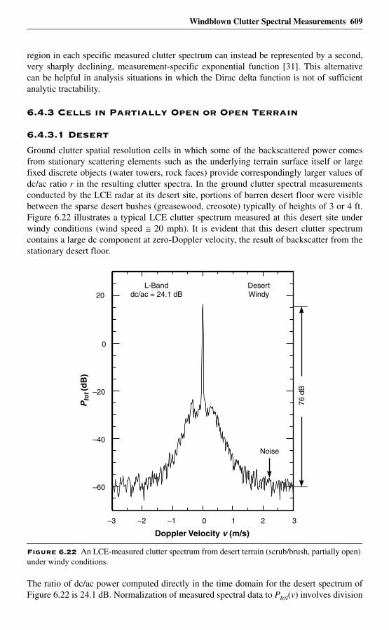
Windblown Clutter Spectral Measurements 609

region in each specific measured clutter spectrum can instead be represented by a second,very sharply declining, measurement-specific exponential function [31]. This alternativecan be helpful in analysis situations in which the Dirac delta function is not of sufficientanalytic tractability.

6.4.3 Cells in Partially Open or Open Terrain

6.4.3.1 Desert

Ground clutter spatial resolution cells in which some of the backscattered power comesfrom stationary scattering elements such as the underlying terrain surface itself or largefixed discrete objects (water towers, rock faces) provide correspondingly larger values ofdc/ac ratio r in the resulting clutter spectra. In the ground clutter spectral measurementsconducted by the LCE radar at its desert site, portions of barren desert floor were visiblebetween the sparse desert bushes (greasewood, creosote) typically of heights of 3 or 4 ft.Figure 6.22 illustrates a typical LCE clutter spectrum measured at this desert site underwindy conditions (wind speed ≅ 20 mph). It is evident that this desert clutter spectrumcontains a large dc component at zero-Doppler velocity, the result of backscatter from thestationary desert floor.

The ratio of dc/ac power computed directly in the time domain for the desert spectrum ofFigure 6.22 is 24.1 dB. Normalization of measured spectral data to Ptot(v) involves division

Figure 6.22 An LCE-measured clutter spectrum from desert terrain (scrub/brush, partially open) under windy conditions.

–2 0 2

–60

–40

–20

0

20

Doppler Velocity v (m/s)

Pto

t (d

B)

76

dB

3–3

DesertWindy

L-Banddc/ac = 24.1 dB

–1 1

Noise

610 Windblown Clutter Spectral Measurements

of power per resolution cell by the width of the cell ∆v. For the data of Figure 6.22, ∆vequals –16.22 dB, so this procedure raises the power in each cell by 16.22 dB. For spectralike that of this figure with a large dc component, the power in the zero-Doppler cell is notdistributed over ∆v but exists as a singular dc component. Reducing the zero-Doppler peakby 16.2 dB allows more straightforward interpretation of r = 24.1 dB as simply the ratio ofthe reduced zero-Doppler peak to the total ac power (i.e., the power level of the stepfunction existing in the unit interval –0.5 < v < +0.5 m/s and containing the same total acspectral power as the measured spectrum).

The desert/windy clutter spectrum of Figure 6.22 contains extensive ac spectral spreading atlower power levels. The low-level ac spectral spreading in these data is due to wind-inducedmotion of the desert foliage. Other LCE-measured desert spectra from similar cells underlight or calm wind conditions showed little or no spectral spreading over as much as 80 dB ofspectral dynamic range [see Figure 6.4(a)]. Unlike the forest/light wind spectrum of Figure6.16, which also contains a large dc component but in which the spectral power decaysrapidly but broadens continuously away from the zero-Doppler peak, the dc component in thedesert/windy spectrum of Figure 6.22 exists more as a discrete delta function at the spectralresolution of the window function over the higher levels of spectral power.

Figure 6.23 shows the ac spectral tail region of the desert/windy spectrum of Figure 6.22 athigher Doppler velocities as 10 log Pac(v) vs log v. Also shown in Figure 6.23 is the forest/windy spectrum previously shown in Figure 6.5. Both measured spectra in Figure 6.23 arenormalized to Pac(v). The 24-dB dc/ac ratio in the desert spectrum (a) of Figure 6.23 resultsin an effective 24-dB loss of sensitivity (i.e., higher noise level) compared with the forestspectrum (b) in measuring ac spectral shape. Otherwise, the ac spectral shape of the desert/windy spectrum in Figure 6.23 almost exactly overlays that of the forest/windy spectrumover their common interval of available spectral dynamic range.

It was previously shown that the exponential shape factor β = 5.2 provides an excellentmatch to the forest/windy spectrum of Figure 6.23. On the basis of these data, thewindblown clutter ac spectral shape that applies for densely forest-vegetated clutter cellsunder windy conditions also applies for more open desert-vegetated cells. That is, these datasuggest that the ac spectral shape function caused by windblown vegetation in a cell may be,at least to a first-order approximation, somewhat independent of the type of vegetation in thecell. However, this equivalence does not extend to include dc/ac ratio; the dc to ac ratio ofclutter spectral power is much higher in partially open desert than in forest terrain.

Knolls, Utah. Figure 6.24 shows X-band desert clutter spectra measured by the PhaseOne radar at two western U. S. desert measurement sites—Booker Mt., Nevada, andKnolls, Utah—in summer season. At both sites these spectra were obtained as eight-gateaverages, 15 FFTs per gate (2,048-point FFTs, PRF = 500 Hz, hor. pol., gate width = pulselength = 150 m). The Booker Mt. spectrum of Figure 6.24(a) was measured from barrenlevel mud flats under calm wind conditions and light rain at 12- to 13.2-km range and 2.3°grazing angle. This Booker Mt. spectrum shows essentially no spectral spreading beyondthe window-function resolution over a 60-dB spectral dynamic range (except for the smallresidual spur indicated at the base of the dc-spike 56 dB down), and again evidences thefield capability of the Phase One radar for making X-band clutter spectral measurements atlow Doppler frequencies [compare with Figure 6.4(c)].

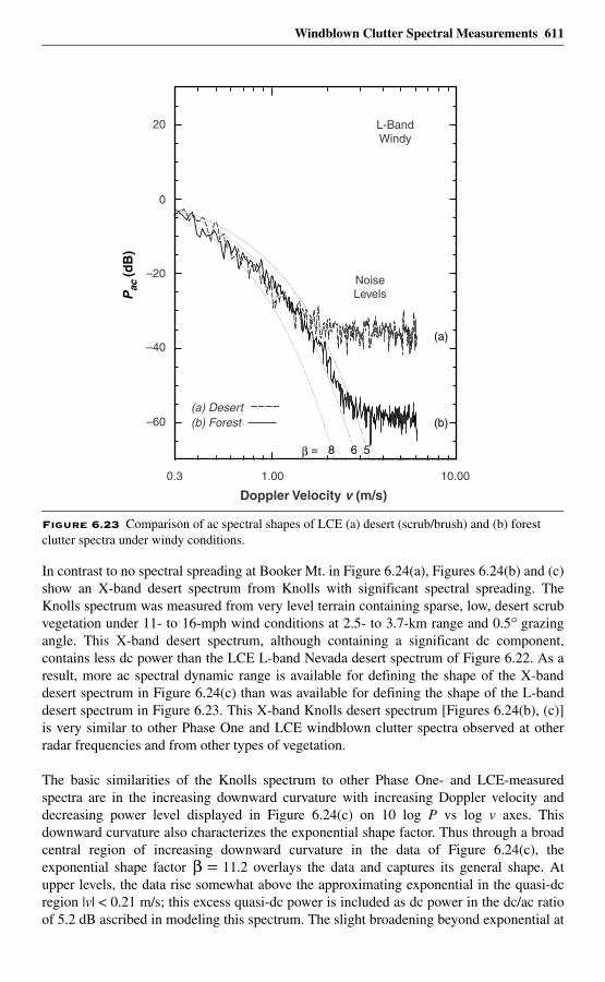
Windblown Clutter Spectral Measurements 611

In contrast to no spectral spreading at Booker Mt. in Figure 6.24(a), Figures 6.24(b) and (c)show an X-band desert spectrum from Knolls with significant spectral spreading. TheKnolls spectrum was measured from very level terrain containing sparse, low, desert scrubvegetation under 11- to 16-mph wind conditions at 2.5- to 3.7-km range and 0.5° grazingangle. This X-band desert spectrum, although containing a significant dc component,contains less dc power than the LCE L-band Nevada desert spectrum of Figure 6.22. As aresult, more ac spectral dynamic range is available for defining the shape of the X-banddesert spectrum in Figure 6.24(c) than was available for defining the shape of the L-banddesert spectrum in Figure 6.23. This X-band Knolls desert spectrum [Figures 6.24(b), (c)]is very similar to other Phase One and LCE windblown clutter spectra observed at otherradar frequencies and from other types of vegetation.

The basic similarities of the Knolls spectrum to other Phase One- and LCE-measuredspectra are in the increasing downward curvature with increasing Doppler velocity anddecreasing power level displayed in Figure 6.24(c) on 10 log P vs log v axes. Thisdownward curvature also characterizes the exponential shape factor. Thus through a broadcentral region of increasing downward curvature in the data of Figure 6.24(c), theexponential shape factor β = 11.2 overlays the data and captures its general shape. Atupper levels, the data rise somewhat above the approximating exponential in the quasi-dcregion |v| < 0.21 m/s; this excess quasi-dc power is included as dc power in the dc/ac ratioof 5.2 dB ascribed in modeling this spectrum. The slight broadening beyond exponential at

Figure 6.23 Comparison of ac spectral shapes of LCE (a) desert (scrub/brush) and (b) forest clutter spectra under windy conditions.

0.3 1.00 10.00

–60

–40

–20

0

20

Doppler Velocity v (m/s)

Pac

(dB

)

(a) Desert(b) Forest

L-BandWindy

NoiseLevels

(a)

(b)

β = 8 6 5

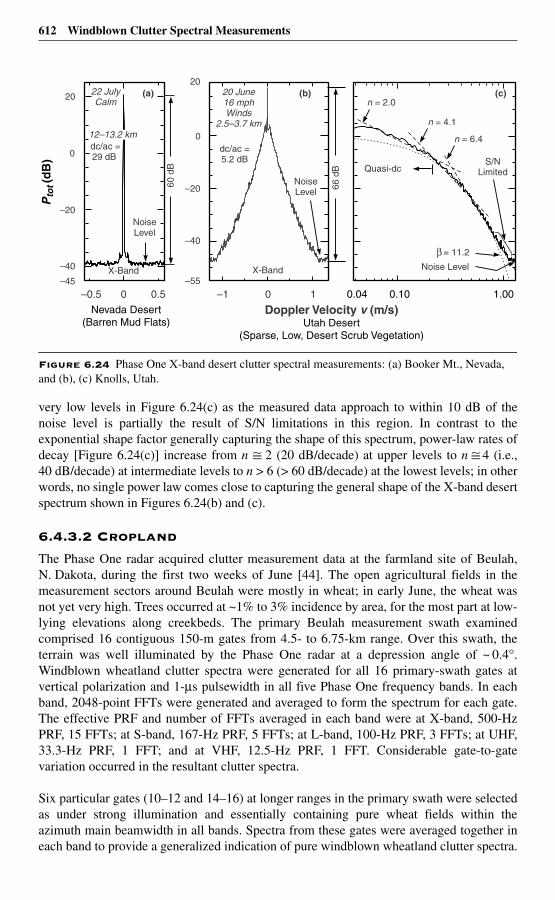
612 Windblown Clutter Spectral Measurements

very low levels in Figure 6.24(c) as the measured data approach to within 10 dB of thenoise level is partially the result of S/N limitations in this region. In contrast to theexponential shape factor generally capturing the shape of this spectrum, power-law rates ofdecay [Figure 6.24(c)] increase from n ≅ 2 (20 dB/decade) at upper levels to n ≅ 4 (i.e.,40 dB/decade) at intermediate levels to n > 6 (> 60 dB/decade) at the lowest levels; in otherwords, no single power law comes close to capturing the general shape of the X-band desertspectrum shown in Figures 6.24(b) and (c).

6.4.3.2 Cropland

The Phase One radar acquired clutter measurement data at the farmland site of Beulah,N. Dakota, during the first two weeks of June [44]. The open agricultural fields in themeasurement sectors around Beulah were mostly in wheat; in early June, the wheat wasnot yet very high. Trees occurred at ~1% to 3% incidence by area, for the most part at low-lying elevations along creekbeds. The primary Beulah measurement swath examinedcomprised 16 contiguous 150-m gates from 4.5- to 6.75-km range. Over this swath, theterrain was well illuminated by the Phase One radar at a depression angle of ~ 0.4°.Windblown wheatland clutter spectra were generated for all 16 primary-swath gates atvertical polarization and 1-µs pulsewidth in all five Phase One frequency bands. In eachband, 2048-point FFTs were generated and averaged to form the spectrum for each gate.The effective PRF and number of FFTs averaged in each band were at X-band, 500-HzPRF, 15 FFTs; at S-band, 167-Hz PRF, 5 FFTs; at L-band, 100-Hz PRF, 3 FFTs; at UHF,33.3-Hz PRF, 1 FFT; and at VHF, 12.5-Hz PRF, 1 FFT. Considerable gate-to-gatevariation occurred in the resultant clutter spectra.

Six particular gates (10–12 and 14–16) at longer ranges in the primary swath were selectedas under strong illumination and essentially containing pure wheat fields within theazimuth main beamwidth in all bands. Spectra from these gates were averaged together ineach band to provide a generalized indication of pure windblown wheatland clutter spectra.

Figure 6.24 Phase One X-band desert clutter spectral measurements: (a) Booker Mt., Nevada, and (b), (c) Knolls, Utah.

0

–20

0

20

Pto

t (d

B)

60

dB

0.5–0.5

X-Band

0

66

dB

–1 1

20 June16 mphWinds

2.5–3.7 km

dc/ac =5.2 dB

X-Band

n = 2.0

–40

–45

–40

–20

20

–55

0

Doppler Velocity v (m/s)Utah Desert

(Sparse, Low, Desert Scrub Vegetation)

(a)

NoiseLevel

NoiseLevel

Noise Level

S/NLimited

(b)

0.04 0.10 1.00

n = 4.1

(c)

n = 6.4

= 11.2

Nevada Desert(Barren Mud Flats)

Quasi-dc

12–13.2 kmdc/ac =29 dB

22 JulyCalm

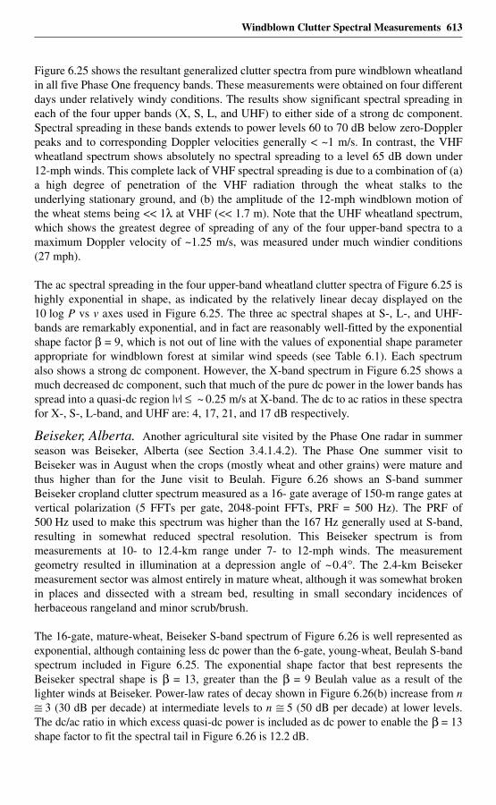
Windblown Clutter Spectral Measurements 613

Figure 6.25 shows the resultant generalized clutter spectra from pure windblown wheatlandin all five Phase One frequency bands. These measurements were obtained on four differentdays under relatively windy conditions. The results show significant spectral spreading ineach of the four upper bands (X, S, L, and UHF) to either side of a strong dc component.Spectral spreading in these bands extends to power levels 60 to 70 dB below zero-Dopplerpeaks and to corresponding Doppler velocities generally < ~1 m/s. In contrast, the VHFwheatland spectrum shows absolutely no spectral spreading to a level 65 dB down under12-mph winds. This complete lack of VHF spectral spreading is due to a combination of (a)a high degree of penetration of the VHF radiation through the wheat stalks to theunderlying stationary ground, and (b) the amplitude of the 12-mph windblown motion ofthe wheat stems being << 1λ at VHF (<< 1.7 m). Note that the UHF wheatland spectrum,which shows the greatest degree of spreading of any of the four upper-band spectra to amaximum Doppler velocity of ~1.25 m/s, was measured under much windier conditions(27 mph).

The ac spectral spreading in the four upper-band wheatland clutter spectra of Figure 6.25 ishighly exponential in shape, as indicated by the relatively linear decay displayed on the10 log P vs v axes used in Figure 6.25. The three ac spectral shapes at S-, L-, and UHF-bands are remarkably exponential, and in fact are reasonably well-fitted by the exponentialshape factor β = 9, which is not out of line with the values of exponential shape parameterappropriate for windblown forest at similar wind speeds (see Table 6.1). Each spectrumalso shows a strong dc component. However, the X-band spectrum in Figure 6.25 shows amuch decreased dc component, such that much of the pure dc power in the lower bands hasspread into a quasi-dc region |v| ≤ ~ 0.25 m/s at X-band. The dc to ac ratios in these spectrafor X-, S-, L-band, and UHF are: 4, 17, 21, and 17 dB respectively.

Beiseker, Alberta. Another agricultural site visited by the Phase One radar in summerseason was Beiseker, Alberta (see Section 3.4.1.4.2). The Phase One summer visit toBeiseker was in August when the crops (mostly wheat and other grains) were mature andthus higher than for the June visit to Beulah. Figure 6.26 shows an S-band summerBeiseker cropland clutter spectrum measured as a 16- gate average of 150-m range gates atvertical polarization (5 FFTs per gate, 2048-point FFTs, PRF = 500 Hz). The PRF of500 Hz used to make this spectrum was higher than the 167 Hz generally used at S-band,resulting in somewhat reduced spectral resolution. This Beiseker spectrum is frommeasurements at 10- to 12.4-km range under 7- to 12-mph winds. The measurementgeometry resulted in illumination at a depression angle of ~0.4°. The 2.4-km Beisekermeasurement sector was almost entirely in mature wheat, although it was somewhat brokenin places and dissected with a stream bed, resulting in small secondary incidences ofherbaceous rangeland and minor scrub/brush.

The 16-gate, mature-wheat, Beiseker S-band spectrum of Figure 6.26 is well represented asexponential, although containing less dc power than the 6-gate, young-wheat, Beulah S-bandspectrum included in Figure 6.25. The exponential shape factor that best represents theBeiseker spectral shape is β = 13, greater than the β = 9 Beulah value as a result of thelighter winds at Beiseker. Power-law rates of decay shown in Figure 6.26(b) increase from n≅ 3 (30 dB per decade) at intermediate levels to n ≅ 5 (50 dB per decade) at lower levels.The dc/ac ratio in which excess quasi-dc power is included as dc power to enable the β = 13shape factor to fit the spectral tail in Figure 6.26 is 12.2 dB.

614 Windblown Clutter Spectral Measurements

The Beiseker 16-gate spectrum of Figure 6.26 is essentially identical in all respects to acorresponding Beulah wheatland 16-gate spectrum35 (not shown). That is, althoughdetailed gate-to-gate differences exist in these data caused by variations in topography,crops, and wind speeds, when averaged over broad 2.4-km swaths these results indicate thatexponential spectral spreading generally occurs in open cropland terrain without much site-specific variation.

de Loor’s Results. Much earlier measurements of clutter spectra from windblown crops(including wheat) made with a noncoherent X-band system were reported by de Loor,Jurriens, and Gravesteijn [45]. The one example shown by de Loor et al. is an ac spectrumfor full-grown wheat under 5- to 7-mph winds of ~ 40-dB spectral dynamic range. This

Figure 6.25 Phase One five-frequency clutter spectra from North Dakota wheatland measured on four different days in early June under strong breezy or windy conditions.

35. Formed from all 16 primary-swath gates at Beulah, not just the six pure-wheat gates for which results are shown in Figure 6.25.

– 1 0 1–60

–40

–20

0

20

–60

–40

–20

0

20

Doppler Velocity v (m/s)

63

dB

67

dB

61

dB

72

dB

65

dB

12 June12 mphwinds

7 June19 mphwinds

8 June14 mphwinds

8 June27 mphwinds

10 June12 mphwinds

v (m/s) v (m/s) v (m/s)–1 10 –1 10

–1 0 1 –1 0 1

Pto

t (d

B)

X-Band S-Band L-Band

Pto

t (d

B)

UHF VHF

N. Dakota Cropland (Wheat)

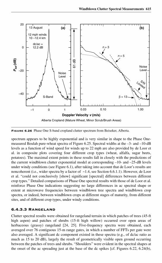
Windblown Clutter Spectral Measurements 615

spectrum appears to be highly exponential and is very similar in shape to the Phase One-measured Beulah pure-wheat spectra of Figure 6.25. Spectral widths at the –3- and –10-dBlevels as a function of wind speed for winds up to 22 mph are also provided by de Loor etal. in composite plots covering four different crop types (wheat, alfalfa, sugar beets,potatoes). The maximal extent points in these results fall in closely with the predictions ofthe current windblown clutter exponential model at corresponding –10- and –25-dB levelsunder windy conditions (see Figure 6.1), after taking into account that de Loor’s results arenoncoherent (i.e., wider spectra by a factor of ~1.4, see Section 6.6.1.1). However, de Looret al. “could not conclusively [show] significant [spectral] differences between differentcrop types.” Detailed comparisons of Phase One spectral results with those of de Loor et al.reinforce Phase One indications suggesting no large differences in ac spectral shape orextent at microwave frequencies between windblown tree spectra and windblown cropspectra, or indeed, between windblown crops at different stages of maturity, from differentsites, and of different crop types, under windy conditions.

6.4.3.3 Rangeland

Clutter spectral results were obtained for rangeland terrain in which patches of trees (45-fthigh aspen) and patches of shrubs (15-ft high willow) occurred over open areas ofherbaceous (grassy) rangeland [24, 25]. Five-frequency spectra were obtained, eachaveraged over 76 contiguous 15-m range gates, in which a number of FFTs per gate werealso averaged. A significant dc component existed in these spectra (e.g., of dc/ac ratio asmuch as 15 to 20 dB), largely the result of geometrically visible open ground occurringbetween the patches of trees and shrubs. “Shoulders” were evident in the spectral shapes atthe onset of the ac spreading just at the base of the dc spikes [cf. Figures 6.22, 6.24(b),

Figure 6.26 Phase One S-band cropland clutter spectrum from Beiseker, Alberta.

0 1

–40

–20

0

20

Pto

t (d

B)

–1

61 d

B

Doppler Velocity v (m/s)

S-Band

13 August

12 mph winds10 –12.4 km

NoiseLevel

(a) (b)

Alberta Cropland (Mature Wheat, Minor Scrub/Brush Areas)

0.03 0.10 1.00

n = 5

β = 13

n = 3dc/ac =12.2 dB

NoiseLevel

S/NLimited

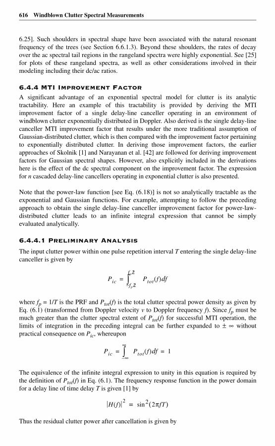
616 Windblown Clutter Spectral Measurements

6.25]. Such shoulders in spectral shape have been associated with the natural resonantfrequency of the trees (see Section 6.6.1.3). Beyond these shoulders, the rates of decayover the ac spectral tail regions in the rangeland spectra were highly exponential. See [25]for plots of these rangeland spectra, as well as other considerations involved in theirmodeling including their dc/ac ratios.

6.4.4 MTI Improvement FactorA significant advantage of an exponential spectral model for clutter is its analytictractability. Here an example of this tractability is provided by deriving the MTIimprovement factor of a single delay-line canceller operating in an environment ofwindblown clutter exponentially distributed in Doppler. Also derived is the single delay-linecanceller MTI improvement factor that results under the more traditional assumption ofGaussian-distributed clutter, which is then compared with the improvement factor pertainingto exponentially distributed clutter. In deriving those improvement factors, the earlierapproaches of Skolnik [1] and Narayanan et al. [42] are followed for deriving improvementfactors for Gaussian spectral shapes. However, also explicitly included in the derivationshere is the effect of the dc spectral component on the improvement factor. The expressionfor n cascaded delay-line cancellers operating in exponential clutter is also presented.

Note that the power-law function [see Eq. (6.18)] is not so analytically tractable as theexponential and Gaussian functions. For example, attempting to follow the precedingapproach to obtain the single delay-line canceller improvement factor for power-law-distributed clutter leads to an infinite integral expression that cannot be simplyevaluated analytically.

6.4.4.1 Preliminary Analysis

The input clutter power within one pulse repetition interval T entering the single delay-linecanceller is given by

where fp = 1/T is the PRF and Ptot(f) is the total clutter spectral power density as given byEq. (6.1) (transformed from Doppler velocity v to Doppler frequency f). Since fp must bemuch greater than the clutter spectral extent of Ptot(f) for successful MTI operation, thelimits of integration in the preceding integral can be further expanded to ± ∞ withoutpractical consequence on Pic, whereupon

The equivalence of the infinite integral expression to unity in this equation is required bythe definition of Ptot(f) in Eq. (6.1). The frequency response function in the power domainfor a delay line of time delay T is given [1] by

Thus the residual clutter power after cancellation is given by

Pic Ptot f( ) fdfp 2⁄–

fp 2⁄

∫=

Pic Ptot f( ) fd∞–

∞

∫ 1= =

H f( ) 2 2 2πfT( )sin=

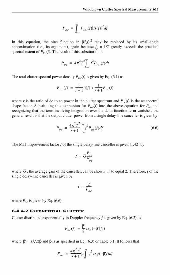
Windblown Clutter Spectral Measurements 617

In this equation, the sine function in |H(f)|2 may be replaced by its small-angleapproximation (i.e., its argument), again because fp = 1/T greatly exceeds the practicalspectral extent of Ptot(f). The result of this substitution is

The total clutter spectral power density Ptot(f) is given by Eq. (6.1) as

where r is the ratio of dc to ac power in the clutter spectrum and Pac(f) is the ac spectralshape factor. Substituting this expression for Ptot(f) into the above equation for Poc andrecognizing that the term involving integration over the delta function term vanishes, thegeneral result is that the output clutter power from a single delay-line canceller is given by

(6.6)

The MTI improvement factor I of the single delay-line canceller is given [1,42] by

where , the average gain of the canceller, can be shown [1] to equal 2. Therefore, I of thesingle delay-line canceller is given by

where Poc is given by Eq. (6.6).

6.4.4.2 Exponential Clutter

Clutter distributed exponentially in Doppler frequency f is given by Eq. (6.2) as

where = (λ/2)β and β is as specified in Eq. (6.3) or Table 6.1. It follows that

Poc Ptot f( ) H f( ) 2fd

∞–

∞

∫=

Poc 4π2T

2f2Ptot f( ) fd

∞–

∞

∫=

Ptot f( ) rr 1+-----------δ f( ) 1

r 1+-----------Pac f( )+=

Poc4π2

T2

r 1+-------------- f

2Pac f( ) fd

∞–

∞

∫=

I GPic

Poc--------=

G

I 2Poc--------=

Pac f( ) β'2--- β'– f( )exp=

β'

Poc4π2

T2

r 1+--------------β' f

2 β– 'f( )exp fd0

∞

∫=

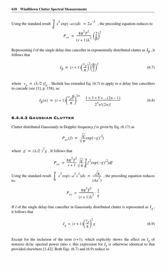
618 Windblown Clutter Spectral Measurements

Using the standard result , the preceding equation reduces to

Representing I of the single delay-line canceller in exponentially distributed clutter as , itfollows that

(6.7)

where . Skolnik has extended Eq. (6.7) to apply to n delay line cancellersin cascade (see [1], p. 158), as:

(6.8)

6.4.4.3 Gaussian Clutter

Clutter distributed Gaussianly in Doppler frequency f is given by Eq. (6.17) as

where . It follows that

Using the standard result , the preceding equation reducesto:

If I of the single delay-line canceller in Gaussianly distributed clutter is represented as ,it follows that

(6.9)

Except for the inclusion of the term (r+1), which explicitly shows the effect on Ig ofnonzero dc/ac spectral power ratio r, this expression for Ig is otherwise identical to thatprovided elsewhere [1,42]. Both Eqs. (6.7) and (6.9) reduce to

x2

ax–( )exp xd0

∞

∫ 2a3–=

Poc8π2

T2

r 1+( )λ2-------------------- 2

β---

2⋅=

Iβ

Iβ r 1+( )vp

π-----

2 β

2---

2=

vp λ 2⁄( )fp=

Iβ n( ) r 1+( )vpβπ

--------

2n

= 1 3 5 ... 2n 1–( )×××

2nn! 2n( )!

----------------------------------------------------

Pac f( ) g'π--- g'f

2–( )exp=

g' λ 2⁄( )2g=

Poc8π2

T2

r 1+--------------- g'

π--- f

2g'f

2–( )exp fd0

∞

∫=

x2

a2x

2–( )exp xd

0

∞

∫ π

4a3( )

------------=

Poc8π2

T2

r 1+( )λ2-------------------- 1

g---⋅=

Ig

Ig r 1+( )vp

π----

2

g=

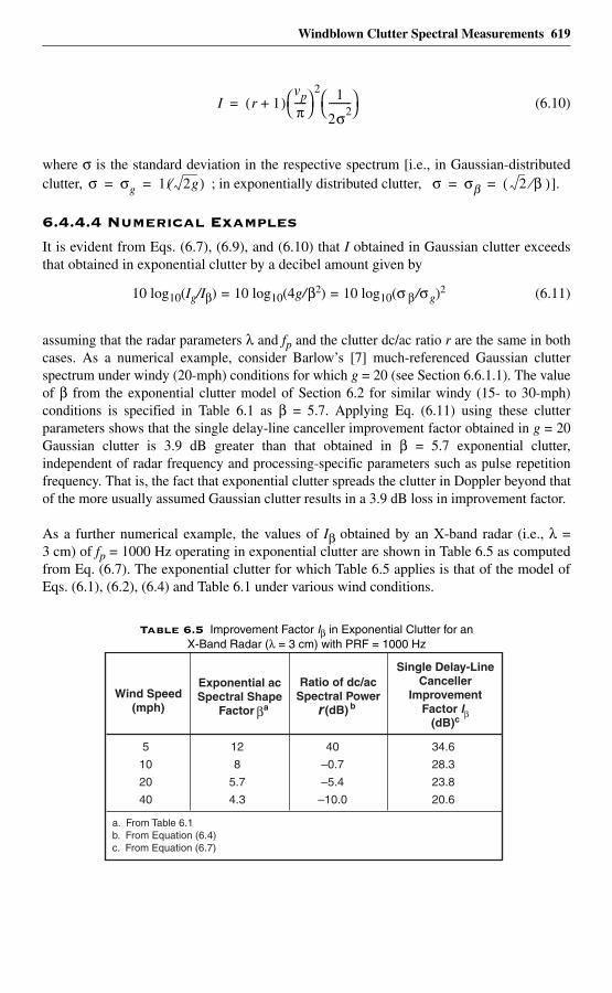
Windblown Clutter Spectral Measurements 619

(6.10)

where σ is the standard deviation in the respective spectrum [i.e., in Gaussian-distributedclutter, ; in exponentially distributed clutter, ].

6.4.4.4 Numerical Examples

It is evident from Eqs. (6.7), (6.9), and (6.10) that I obtained in Gaussian clutter exceedsthat obtained in exponential clutter by a decibel amount given by

10 log10(Ig/Iβ) = 10 log10(4g/β2) = 10 log10(σ β/σg)2 (6.11)

assuming that the radar parameters λ and fp and the clutter dc/ac ratio r are the same in bothcases. As a numerical example, consider Barlow’s [7] much-referenced Gaussian clutterspectrum under windy (20-mph) conditions for which g = 20 (see Section 6.6.1.1). The valueof β from the exponential clutter model of Section 6.2 for similar windy (15- to 30-mph)conditions is specified in Table 6.1 as β = 5.7. Applying Eq. (6.11) using these clutterparameters shows that the single delay-line canceller improvement factor obtained in g = 20Gaussian clutter is 3.9 dB greater than that obtained in β = 5.7 exponential clutter,independent of radar frequency and processing-specific parameters such as pulse repetitionfrequency. That is, the fact that exponential clutter spreads the clutter in Doppler beyond thatof the more usually assumed Gaussian clutter results in a 3.9 dB loss in improvement factor.

As a further numerical example, the values of Iβ obtained by an X-band radar (i.e., λ =3 cm) of fp = 1000 Hz operating in exponential clutter are shown in Table 6.5 as computedfrom Eq. (6.7). The exponential clutter for which Table 6.5 applies is that of the model ofEqs. (6.1), (6.2), (6.4) and Table 6.1 under various wind conditions.

Table 6.5 Improvement Factor Iβ in Exponential Clutter for an X-Band Radar (λ = 3 cm) with PRF = 1000 Hz

I r 1+( )vp

π-----

2 1

2σ2---------

=

σ σg 1 2g( )⁄= = σ σβ 2 β⁄( )= =

Wind Speed(mph)

Exponential acSpectral Shape

Factor

Ratio of dc/acSpectral Power

(dB) r b

Single Delay-LineCanceller

ImprovementFactor Iβ

(dB)c

5

10

20

40

12

8

5.7

4.3

40

–0.7

–5.4

–10.0

34.6

28.3

23.8

20.6

a. From Table 6.1b. From Equation (6.4)c. From Equation (6.7)

βa

620 Windblown Clutter Spectral Measurements

6.5 Impact on MTI and STAP

6.5.1 IntroductionThe shape of the windblown radar ground clutter Doppler spectrum is important indetermining the performance of target detection in ground clutter. In modern radar thatoperates with wide dynamic range and low noise floor, the decay of the spectral tails ofground clutter has significant impact on the detection of small moving targets. In suchsystems, detection performance can be clutter limited, even to relatively high Dopplerfrequencies. Therefore, the rate at which the clutter spectral tails decay (i.e., the spectralshape) with increasing Doppler frequency is an essential issue for the realistic predictionof detection performance.

The preceding section (Section 6.4.4) shows that the use of a realistic exponential groundclutter spectral shape causes significant loss in single-delay-line improvement factor I, e.g.,3.9 dB, compared to use of the more conventional Gaussian ground clutter spectral shape.Section 6.5 expands this previous discussion to consider the impact of ground clutterspectral shape on the prediction of detection performance of ground-based and airbornesurveillance radar using modern coherent signal processing. It is shown that, with suchprocessing, detection losses much greater than 3.9 dB can occur using incorrect clutterspectral shapes for performance prediction. The results presented summarize the work inthis area of Professor Alfonso Farina of Alenia Marconi Systems, Rome, Italy, and hisItalian colleagues, Professor Fulvio Gini and Dr. Maria V. Sabrina Greco at the Universityof Pisa and Professor Pierfrancesco Lombardo at the University of Rome, who took up theLincoln Laboratory findings concerning ground clutter spectral shape and investigated theimpact of these findings on radar signal processing techniques for target detection inclutter. What follows summarizes36 these investigations; for more extensive discussion andresults describing this work, refer to the original technical journal articles [30–33].

Following subsections first review the derivation of how ground clutter spectral shapeaffects the performance of optimum coherent detectors, both for ground-based and airborneearly-warning (AEW) surveillance radars, when such radars operate in a ground clutterenvironment of Rayleigh clutter amplitudes (i.e., I and Q components of Gaussian pdf). Ithas previously been shown in this book that temporal clutter amplitude statistics fromwindblown vegetation (particularly, windblown trees) indeed tend to be Rayleighdistributed—see Figure 5.A.16. The expressions for detection performance in Gaussianclutter, as discussed in what follows, can also apply to adaptive coherent detection innonhomogeneous and nonstationary clutter environments, providing the I and Q clutterpdf’s remain Gaussian [46].

Numerical results are provided both at X-band and L-band in which the predictedperformance of the MTI improvement factor I is compared between using an exponentialshape for the ground clutter spectrum, as illustrated and modeled heretofore in Chapter 6,and using Gaussian and power-law shapes for the ground clutter spectrum, such as havebeen previously employed in the technical literature and which are defined and discussedsubsequently in Section 6.6.1. This allows evaluation of the sensitivity of detection systemperformance prediction to the use of incorrect ground clutter spectral models. It is shown

36. The summary provided here includes material originally published in [30, 31, and 33] by permission of IEEE, and in [32] by permission of IEE.

Windblown Clutter Spectral Measurements 621

that the Gaussian shape can significantly overestimate system performance, whereas thepower-law shape can significantly underestimate system performance, compared to themore correct exponential clutter spectral shape.

6.5.2 Impact on Performance of Optimum MTITo evaluate the impact of the measured clutter Doppler spectrum on the detectionperformance, we proceed as follows. Consider a ground-based surveillance radar in whichthe radar receiver demodulates, filters the incoming narrowband waveform, and uniformlysamples each pulse return, thus obtaining N complex samples {z[i]} spaced by Tseconds, where T = 1/PRF is the PRI. The N samples are assembled into the N-dimensionalvector z = zI + jzQ = [z[0] ... z[N – 1]]T, where zI and zQ represent the vectors of the I and Qcomponents, and the superscript “T” stands for “transpose of.” Assuming an exactknowledge of the clutter covariance matrix, the optimum MTI processor is a coherent lineartransversal filter with complex coefficient vector w = [w1, w2, ..., wN]T. To test a range cellfor detection, the quantity wHz is evaluated (where the superscript “H” stands for“conjugate transpose of”), and the envelope of the result is compared to a detectionthreshold, thus ascertaining whether a target is present or not. The target signal is modeledby the N-dimensional complex-valued vector s = α p, where α is a complex parameteraccounting for target amplitude and initial phase and pi = e j2π i fT, 0 ≤ i ≤ N−1; f being thetarget Doppler frequency. The interference (i.e., clutter plus noise) is given by the vector d,where PC is clutter power; and PN is white noise power. The parameters that characterizethe clutter interference are: the clutter to noise power ratio (CNR), the shape of the clutterspectrum, and the width of the clutter spectrum for given shape. In the results to follow, theshape of the clutter spectrum is specified to be either Gaussian, exponential, or power law;and the width of the clutter spectrum is characterized by either the one-lag autocorrelationcoefficient ρ (X-band results), or by the –3-dB spectral width (L-band results). In allresults, the mean Doppler frequency of the clutter spectrum is assumed to be zero.

The signal to interference power ratio SIRo at the output of the filter is given by:

(6.12)

where S = E {ssH} is the covariance matrix of the target signal and M = E {ddH} = (PC +PN) Mn is the covariance matrix of the interference d (i.e., clutter and noise). Mn is thenormalized covariance matrix, i.e., [Mn]i, i = 1; i = 0, 1, ..., N–1. The performance of thefilter is described by the definition of clutter improvement factor I, as

(6.13)

where SIRi is the signal-to-interference power ratio referred to a single pulse at the input ofthe filter. For the optimum MTI processor (i.e., one having the weight vector w = cM-1p),the improvement factor is given by

Ic = pHMn-1p (6.14)

N 1–i 0=

SIRow

HSw

wH

Mw------------------=

ISIRo

SIRi------------=

622 Windblown Clutter Spectral Measurements

The above discussion is applicable to the one-dimensional (1-D) ground-based case (i.e.,single antenna) parameterized by f only, as opposed to the two-dimensional (2-D) airbornecase (i.e., multiple effective antenna elements) parameterized by f and direction-of-arrival θdiscussed in Section 6.5.3. As will be shown, Eq. (6.14) also applies to the airborne (2-D)case and to Kelly’s adaptive processor [46], for expressions of p and Mn extended to applyto these cases (see Section 6.5.3).

To obtain assigned values of probability of detection PD and probability of false alarm PFA,a specified level of SIRo at the output of the detection filter must be provided. The SIRiwhich is required at the input of this filter (in dB) to ensure the required performance isgiven by SIRi|dB = SIRo|dB – Ic(f)|dB. The improvement factor of the filter is different forany Doppler frequency, while SIRo is constant. Thus a normalized visibility plot is providedby showing [–Ic(f)|dB] for given N. In what follows, two sets of plots are used to representperformance:

(i) visibility curves: the inverse of Ic (i.e., SIRi required to leave SIRo = 0 dB) as a function of the Doppler frequency f for given N;

(ii) improvement factor plots: Ic as a function of N, for given Doppler frequency f.

The visibility curve (the inverse of Ic) is a scaled (normalized) version of the required SIRifor given N as a function of target Doppler frequency necessary to provide a specific SIRoas required, for any given detector and target model, to ensure an assigned performancelevel (for example PD = 0.8 with PFA = 10-6), for the differing clutter spectral shapes. Thatis, the visibility curve allows the determination for given N of the SIRi that is required at theinput of the radar detector to ensure the desired performance as given by SIRi = SIRo/Ic,where SIRo is a constant. The improvement factor plot allows the determination of theminimum number of radar pulses N for given f that is required to provide a desired value ofIc, also for the differing clutter spectral shapes.

6.5.2.1 X-Band Results (1-D)

The X-band results to follow compare optimum MTI filter performance as given by Eq.(6.14) for corresponding Gaussian and exponential windblown ground clutter spectralshapes under breezy wind conditions. The model utilized for clutter power spectral density(PSD) is that specified in Section 6.2, particularly by Eq. (6.1) which specifies Ptot(v) interms of dc/ac ratio r and the ac shape factor Pac(v). The exponential spectral shape ismodeled as specified in Section 6.2.1, particularly by Eq. (6.2) which specifiesexponential spectral shape in terms of the exponential shape parameter β,β beingspecified as a function of wind speed (e.g., breezy, windy) in Table 6.1 and Figure 6.1. TheGaussian spectral shape is modeled as specified by Eq. (6.17) in Section 6.6.1.1, where theGaussian shape parameter g is that required to give the same one-lag temporalautocorrelation coefficient ρ as that of the exponential spectrum under given windconditions. This procedure is one way of normalizing the Gaussian and exponential shapesto be of equivalent extent in Doppler as a function of wind speed, the autocorrelationfunction being the inverse Fourier transform of the clutter power spectrum. The dc/ac ratior in the clutter spectrum is modeled as specified in Section 6.2.2, particular by Eq. (6.4)which models r as a function of wind speed w and radar carrier frequency fo (see alsoFigure 6.2). In the results to follow, fo = 9.2 GHz (X-band), PRF = 1/T = 500 Hz, and CNR= 50 dB.

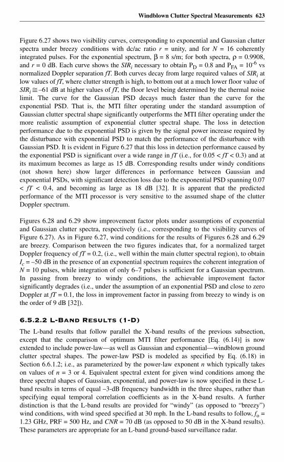
Windblown Clutter Spectral Measurements 623

Figure 6.27 shows two visibility curves, corresponding to exponential and Gaussian clutterspectra under breezy conditions with dc/ac ratio r = unity, and for N = 16 coherentlyintegrated pulses. For the exponential spectrum, β = 8 s/m; for both spectra, ρ = 0.9908,and r = 0 dB. Each curve shows the SIRi necessary to obtain PD = 0.8 and PFA = 10-6 vsnormalized Doppler separation fT. Both curves decay from large required values of SIRi atlow values of fT, where clutter strength is high, to bottom out at a much lower floor value ofSIRi ≅ –61 dB at higher values of fT, the floor level being determined by the thermal noiselimit. The curve for the Gaussian PSD decays much faster than the curve for theexponential PSD. That is, the MTI filter operating under the standard assumption ofGaussian clutter spectral shape significantly outperforms the MTI filter operating under themore realistic assumption of exponential clutter spectral shape. The loss in detectionperformance due to the exponential PSD is given by the signal power increase required bythe disturbance with exponential PSD to match the performance of the disturbance withGaussian PSD. It is evident in Figure 6.27 that this loss in detection performance caused bythe exponential PSD is significant over a wide range in fT (i.e., for 0.05 < fT < 0.3) and atits maximum becomes as large as 15 dB. Corresponding results under windy conditions(not shown here) show larger differences in performance between Gaussian andexponential PSDs, with significant detection loss due to the exponential PSD spanning 0.07< fT < 0.4, and becoming as large as 18 dB [32]. It is apparent that the predictedperformance of the MTI processor is very sensitive to the assumed shape of the clutterDoppler spectrum.

Figures 6.28 and 6.29 show improvement factor plots under assumptions of exponentialand Gaussian clutter spectra, respectively (i.e., corresponding to the visibility curves ofFigure 6.27). As in Figure 6.27, wind conditions for the results of Figures 6.28 and 6.29are breezy. Comparison between the two figures indicates that, for a normalized targetDoppler frequency of fT = 0.2, (i.e., well within the main clutter spectral region), to obtainIc = –50 dB in the presence of an exponential spectrum requires the coherent integration ofN = 10 pulses, while integration of only 6–7 pulses is sufficient for a Gaussian spectrum.In passing from breezy to windy conditions, the achievable improvement factorsignificantly degrades (i.e., under the assumption of an exponential PSD and close to zeroDoppler at fT = 0.1, the loss in improvement factor in passing from breezy to windy is onthe order of 9 dB [32]).

6.5.2.2 L-Band Results (1-D)

The L-band results that follow parallel the X-band results of the previous subsection,except that the comparison of optimum MTI filter performance [Eq. (6.14)] is nowextended to include power-law—as well as Gaussian and exponential—windblown groundclutter spectral shapes. The power-law PSD is modeled as specified by Eq. (6.18) inSection 6.6.1.2; i.e., as parameterized by the power-law exponent n which typically takeson values of n = 3 or 4. Equivalent spectral extent for given wind conditions among thethree spectral shapes of Gaussian, exponential, and power-law is now specified in these L-band results in terms of equal –3-dB frequency bandwidth in the three shapes, rather thanspecifying equal temporal correlation coefficients as in the X-band results. A furtherdistinction is that the L-band results are provided for “windy” (as opposed to “breezy”)wind conditions, with wind speed specified at 30 mph. In the L-band results to follow, fo =1.23 GHz, PRF = 500 Hz, and CNR = 70 dB (as opposed to 50 dB in the X-band results).These parameters are appropriate for an L-band ground-based surveillance radar.

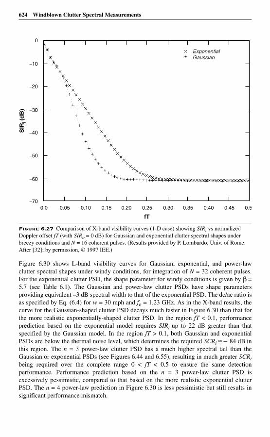
624 Windblown Clutter Spectral Measurements

Figure 6.30 shows L-band visibility curves for Gaussian, exponential, and power-lawclutter spectral shapes under windy conditions, for integration of N = 32 coherent pulses.For the exponential clutter PSD, the shape parameter for windy conditions is given by β =5.7 (see Table 6.1). The Gaussian and power-law clutter PSDs have shape parametersproviding equivalent –3 dB spectral width to that of the exponential PSD. The dc/ac ratio isas specified by Eq. (6.4) for w = 30 mph and fo = 1.23 GHz. As in the X-band results, thecurve for the Gaussian-shaped clutter PSD decays much faster in Figure 6.30 than that forthe more realistic exponentially-shaped clutter PSD. In the region fT < 0.1, performanceprediction based on the exponential model requires SIRi up to 22 dB greater than thatspecified by the Gaussian model. In the region fT > 0.1, both Gaussian and exponentialPSDs are below the thermal noise level, which determines the required SCRi ≅ − 84 dB inthis region. The n = 3 power-law clutter PSD has a much higher spectral tail than theGaussian or exponential PSDs (see Figures 6.44 and 6.55), resulting in much greater SCRibeing required over the complete range 0 < fT < 0.5 to ensure the same detectionperformance. Performance prediction based on the n = 3 power-law clutter PSD isexcessively pessimistic, compared to that based on the more realistic exponential clutterPSD. The n = 4 power-law prediction in Figure 6.30 is less pessimistic but still results insignificant performance mismatch.

Figure 6.27 Comparison of X-band visibility curves (1-D case) showing SIRi vs normalized Doppler offset fT (with SIRo = 0 dB) for Gaussian and exponential clutter spectral shapes under breezy conditions and N = 16 coherent pulses. (Results provided by P. Lombardo, Univ. of Rome. After [32]; by permission, © 1997 IEE.)

0.0–70

–60

0.05

SIR

i (d

B)

fT

0.10 0.15 0.20 0.25 0.30 0.35 0.40 0.45 0.5

–50

–40

–30

–20

–10

0

ExponentialGaussian

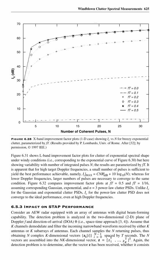
Windblown Clutter Spectral Measurements 625

Figure 6.31 shows L-band improvement factor plots for clutter of exponential spectral shapeunder windy conditions (i.e., corresponding to the exponential curve of Figure 6.30) but hereshowing variability with number of integrated pulses N; the results are parameterized by fT. Itis apparent that for high target Doppler frequencies, a small number of pulses is sufficient toyield the best performance achievable, namely, Ic|MAX = CNR|dB + 10 log10(N); whereas forlower Doppler frequencies, larger numbers of pulses are necessary to converge to the samecondition. Figure 6.32 compares improvement factor plots at fT = 0.5 and fT = 1/16,assuming corresponding Gaussian, exponential, and n = 3 power-law clutter PSDs. Unlike Icfor the Gaussian and exponential clutter PSDs, Ic for the power-law clutter PSD does notconverge to the ideal performance, even at high Doppler frequencies.

6.5.3 Impact on STAP PerformanceConsider an AEW radar equipped with an array of antennas with digital beam-formingcapability. The detection problem is analyzed in the two-dimensional (2-D) plane ofDoppler f and direction-of-arrival (DOA) θ (i.e., space-time approach [3, 4]). Assume thatK channels demodulate and filter the incoming narrowband waveform received by either Kantennas or K subarrays of antennas. Each channel samples the N returning pulses, thusobtaining N complex K-dimensional vectors {zk[i]} spaced by T seconds. The Nvectors are assembled into the NK-dimensional vector, , ..., ]T. Again, thedetection problem is to determine, after the vector z has been received, whether it consists

Figure 6.28 X-band improvement factor plots (1-D case) showing Ic vs N for breezy exponential clutter, parameterized by fT. (Results provided by P. Lombardo, Univ. of Rome. After [32]; by permission, © 1997 IEE.)

0

10

5

I c (

dB

)

Number of Coherent Pulses, N

10 15 20 25 30

20

30

40

50

60

70

fT = 0.0

fT = 0.1fT = 0.2

fT = 0.3fT = 0.4fT = 0.5

N 1–i 0=

z z1T[= zK

T

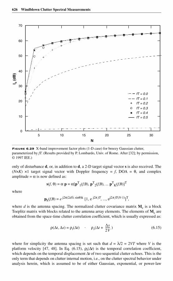
626 Windblown Clutter Spectral Measurements

only of disturbance d, or, in addition to d, a 2-D target signal vector s is also received. The(N×K) ×1 target signal vector with Doppler frequency = f, DOA = θ, and complexamplitude = α is now defined as:

s(f, θ) = α p = α[pT1(f,θ), pT

2(f,θ), ... pTK(f,θ)]T

where

pk(f,θ) = e j2π(2d/λ sinθ)k [1, e j2π fT, ..., ej2π fT(N-1)]T,

where d is the antenna spacing. The normalized clutter covariance matrix Mc is a blockToeplitz matrix with blocks related to the antenna array elements. The elements of Mc areobtained from the space-time clutter correlation coefficient, which is usually expressed as:

ρ(∆t, ∆s) = ρt(∆t) ρs(∆t + ) (6.15)

where for simplicity the antenna spacing is set such that d = λ/2 = 2VT where V is theplatform velocity [47, 48]. In Eq. (6.15), ρt(∆t) is the temporal correlation coefficient,which depends on the temporal displacement ∆t of two sequential clutter echoes. This is theonly term that depends on clutter internal motion, i.e., on the clutter spectral behavior underanalysis herein, which is assumed to be of either Gaussian, exponential, or power-law

Figure 6.29 X-band improvement factor plots (1-D case) for breezy Gaussian clutter, parameterized by fT. (Results provided by P. Lombardo, Univ. of Rome. After [32]; by permission,© 1997 IEE.)

0

10

5

I c (

dB

)

N

10 15 20 25 30

20

30

40

50

60

70

fT = 0.0

fT = 0.1fT = 0.2

fT = 0.3fT = 0.4fT = 0.5

⋅ ∆s2V-------

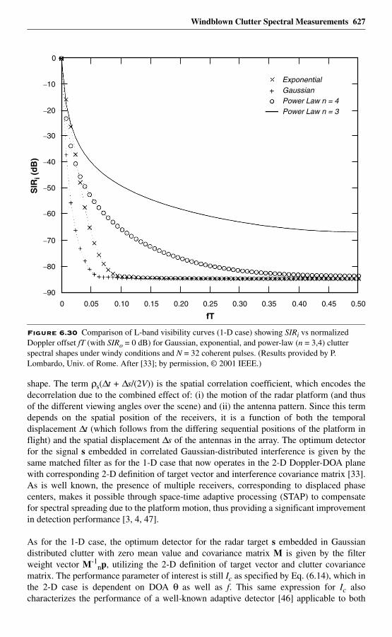
Windblown Clutter Spectral Measurements 627

shape. The term ρs(∆t + ∆s/(2V)) is the spatial correlation coefficient, which encodes thedecorrelation due to the combined effect of: (i) the motion of the radar platform (and thusof the different viewing angles over the scene) and (ii) the antenna pattern. Since this termdepends on the spatial position of the receivers, it is a function of both the temporaldisplacement ∆t (which follows from the differing sequential positions of the platform inflight) and the spatial displacement ∆s of the antennas in the array. The optimum detectorfor the signal s embedded in correlated Gaussian-distributed interference is given by thesame matched filter as for the 1-D case that now operates in the 2-D Doppler-DOA planewith corresponding 2-D definition of target vector and interference covariance matrix [33].As is well known, the presence of multiple receivers, corresponding to displaced phasecenters, makes it possible through space-time adaptive processing (STAP) to compensatefor spectral spreading due to the platform motion, thus providing a significant improvementin detection performance [3, 4, 47].

As for the 1-D case, the optimum detector for the radar target s embedded in Gaussiandistributed clutter with zero mean value and covariance matrix M is given by the filterweight vector M-1

np, utilizing the 2-D definition of target vector and clutter covariancematrix. The performance parameter of interest is still Ic as specified by Eq. (6.14), which inthe 2-D case is dependent on DOA θ as well as f. This same expression for Ic alsocharacterizes the performance of a well-known adaptive detector [46] applicable to both

Figure 6.30 Comparison of L-band visibility curves (1-D case) showing SIRi vs normalized Doppler offset fT (with SIRo = 0 dB) for Gaussian, exponential, and power-law (n = 3,4) clutter spectral shapes under windy conditions and N = 32 coherent pulses. (Results provided by P. Lombardo, Univ. of Rome. After [33]; by permission, © 2001 IEEE.)

0.050

SIR

i (d

B)

fT

0.150.10 0.20 0.25 0.30 0.35 0.40 0.45 0.50

–20

–30

–40

–50

–60

–70

–80

–90

–10

0

ExponentialGaussianPower Law n = 4Power Law n = 3

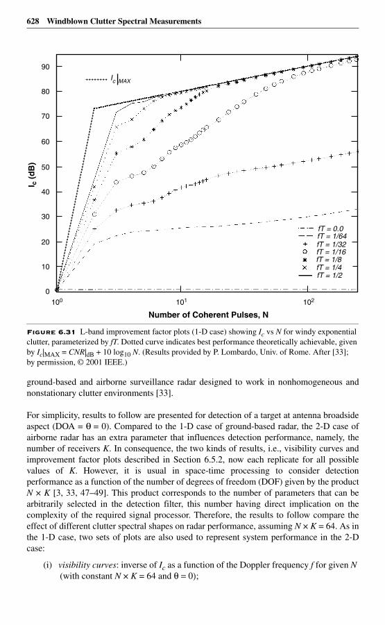
628 Windblown Clutter Spectral Measurements

ground-based and airborne surveillance radar designed to work in nonhomogeneous andnonstationary clutter environments [33].

For simplicity, results to follow are presented for detection of a target at antenna broadsideaspect (DOA = θ = 0). Compared to the 1-D case of ground-based radar, the 2-D case ofairborne radar has an extra parameter that influences detection performance, namely, thenumber of receivers K. In consequence, the two kinds of results, i.e., visibility curves andimprovement factor plots described in Section 6.5.2, now each replicate for all possiblevalues of K. However, it is usual in space-time processing to consider detectionperformance as a function of the number of degrees of freedom (DOF) given by the productN × K [3, 33, 47–49]. This product corresponds to the number of parameters that can bearbitrarily selected in the detection filter, this number having direct implication on thecomplexity of the required signal processor. Therefore, the results to follow compare theeffect of different clutter spectral shapes on radar performance, assuming N × K = 64. As inthe 1-D case, two sets of plots are also used to represent system performance in the 2-Dcase:

(i) visibility curves: inverse of Ic as a function of the Doppler frequency f for given N (with constant N × K = 64 and θ = 0);

Figure 6.31 L-band improvement factor plots (1-D case) showing Ic vs N for windy exponential clutter, parameterized by fT. Dotted curve indicates best performance theoretically achievable, given by Ic|MAX = CNR|dB + 10 log10 N. (Results provided by P. Lombardo, Univ. of Rome. After [33]; by permission, © 2001 IEEE.)

100

I c (

dB

)

Number of Coherent Pulses, N

101 102

90

80

70

60

50

40

30

20

10

0

fT = 0.0fT = 1/64

Ic MAX

fT = 1/32fT = 1/16fT = 1/8fT = 1/4fT = 1/2

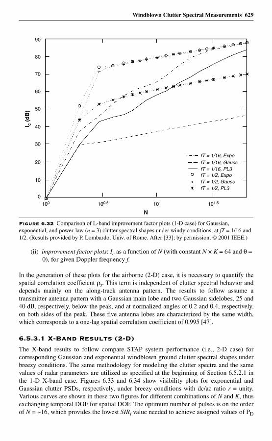
Windblown Clutter Spectral Measurements 629

(ii) improvement factor plots: Ic as a function of N (with constant N × K = 64 and θ = 0), for given Doppler frequency f.

In the generation of these plots for the airborne (2-D) case, it is necessary to quantify thespatial correlation coefficient ρs. This term is independent of clutter spectral behavior anddepends mainly on the along-track antenna pattern. The results to follow assume atransmitter antenna pattern with a Gaussian main lobe and two Gaussian sidelobes, 25 and40 dB, respectively, below the peak, and at normalized angles of 0.2 and 0.4, respectively,on both sides of the peak. These five antenna lobes are characterized by the same width,which corresponds to a one-lag spatial correlation coefficient of 0.995 [47].

6.5.3.1 X-Band Results (2-D)

The X-band results to follow compare STAP system performance (i.e., 2-D case) forcorresponding Gaussian and exponential windblown ground clutter spectral shapes underbreezy conditions. The same methodology for modeling the clutter spectra and the samevalues of radar parameters are utilized as specified at the beginning of Section 6.5.2.1 inthe 1-D X-band case. Figures 6.33 and 6.34 show visibility plots for exponential andGaussian clutter PSDs, respectively, under breezy conditions with dc/ac ratio r = unity.Various curves are shown in these two figures for different combinations of N and K, thusexchanging temporal DOF for spatial DOF. The optimum number of pulses is on the orderof N = ~16, which provides the lowest SIRi value needed to achieve assigned values of PD

Figure 6.32 Comparison of L-band improvement factor plots (1-D case) for Gaussian, exponential, and power-law (n = 3) clutter spectral shapes under windy conditions, at fT = 1/16 and 1/2. (Results provided by P. Lombardo, Univ. of Rome. After [33]; by permission, © 2001 IEEE.)

100

I c (

dB

)

N

101100.5 101.5

90

80

70

60

50

40

30

20

10

0

fT = 1/16, ExpofT = 1/16, GaussfT = 1/16, PL3fT = 1/2, ExpofT = 1/2, GaussfT = 1/2, PL3

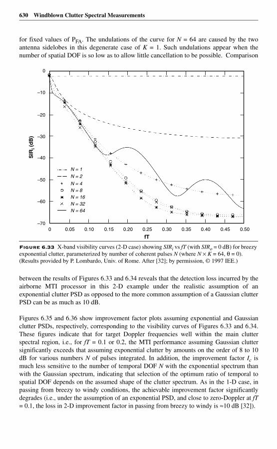
630 Windblown Clutter Spectral Measurements

for fixed values of PFA. The undulations of the curve for N = 64 are caused by the twoantenna sidelobes in this degenerate case of K = 1. Such undulations appear when thenumber of spatial DOF is so low as to allow little cancellation to be possible. Comparison

between the results of Figures 6.33 and 6.34 reveals that the detection loss incurred by theairborne MTI processor in this 2-D example under the realistic assumption of anexponential clutter PSD as opposed to the more common assumption of a Gaussian clutterPSD can be as much as 10 dB.

Figures 6.35 and 6.36 show improvement factor plots assuming exponential and Gaussianclutter PSDs, respectively, corresponding to the visibility curves of Figures 6.33 and 6.34.These figures indicate that for target Doppler frequencies well within the main clutterspectral region, i.e., for fT = 0.1 or 0.2, the MTI performance assuming Gaussian cluttersignificantly exceeds that assuming exponential clutter by amounts on the order of 8 to 10dB for various numbers N of pulses integrated. In addition, the improvement factor Ic ismuch less sensitive to the number of temporal DOF N with the exponential spectrum thanwith the Gaussian spectrum, indicating that selection of the optimum ratio of temporal tospatial DOF depends on the assumed shape of the clutter spectrum. As in the 1-D case, inpassing from breezy to windy conditions, the achievable improvement factor significantlydegrades (i.e., under the assumption of an exponential PSD, and close to zero-Doppler at fT= 0.1, the loss in 2-D improvement factor in passing from breezy to windy is ≈10 dB [32]).

Figure 6.33 X-band visibility curves (2-D case) showing SIRi vs fT (with SIRo = 0 dB) for breezy exponential clutter, parameterized by number of coherent pulses N (where N × K = 64, θ = 0). (Results provided by P. Lombardo, Univ. of Rome. After [32]; by permission, © 1997 IEE.)

SIR

i (d

B)

fT0.050 0.10 0.15 0.20 0.25 0.30 0.35 0.40 0.45 0.50

0

–10

–20

–30

–40

–50

–60

–70

N = 1

N = 2

N = 4N = 8N = 16N = 32N = 64

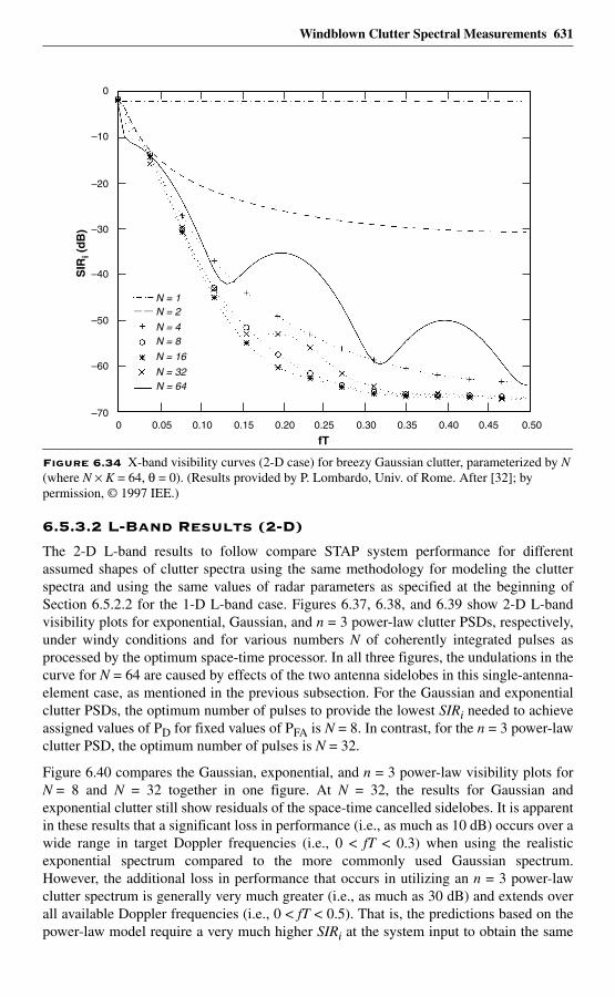
Windblown Clutter Spectral Measurements 631

6.5.3.2 L-Band Results (2-D)

The 2-D L-band results to follow compare STAP system performance for differentassumed shapes of clutter spectra using the same methodology for modeling the clutterspectra and using the same values of radar parameters as specified at the beginning ofSection 6.5.2.2 for the 1-D L-band case. Figures 6.37, 6.38, and 6.39 show 2-D L-bandvisibility plots for exponential, Gaussian, and n = 3 power-law clutter PSDs, respectively,under windy conditions and for various numbers N of coherently integrated pulses asprocessed by the optimum space-time processor. In all three figures, the undulations in thecurve for N = 64 are caused by effects of the two antenna sidelobes in this single-antenna-element case, as mentioned in the previous subsection. For the Gaussian and exponentialclutter PSDs, the optimum number of pulses to provide the lowest SIRi needed to achieveassigned values of PD for fixed values of PFA is N = 8. In contrast, for the n = 3 power-lawclutter PSD, the optimum number of pulses is N = 32.

Figure 6.40 compares the Gaussian, exponential, and n = 3 power-law visibility plots forN = 8 and N = 32 together in one figure. At N = 32, the results for Gaussian andexponential clutter still show residuals of the space-time cancelled sidelobes. It is apparentin these results that a significant loss in performance (i.e., as much as 10 dB) occurs over awide range in target Doppler frequencies (i.e., 0 < fT < 0.3) when using the realisticexponential spectrum compared to the more commonly used Gaussian spectrum.However, the additional loss in performance that occurs in utilizing an n = 3 power-lawclutter spectrum is generally very much greater (i.e., as much as 30 dB) and extends overall available Doppler frequencies (i.e., 0 < fT < 0.5). That is, the predictions based on thepower-law model require a very much higher SIRi at the system input to obtain the same

Figure 6.34 X-band visibility curves (2-D case) for breezy Gaussian clutter, parameterized by N (where N × K = 64, θ = 0). (Results provided by P. Lombardo, Univ. of Rome. After [32]; by permission, © 1997 IEE.)

SIR

i (d

B)

fT0.050 0.10 0.15 0.20 0.25 0.30 0.35 0.40 0.45 0.50

0

–10

–20

–30

–40

–50

–60

–70

N = 1N = 2

N = 4N = 8

N = 16

N = 32N = 64

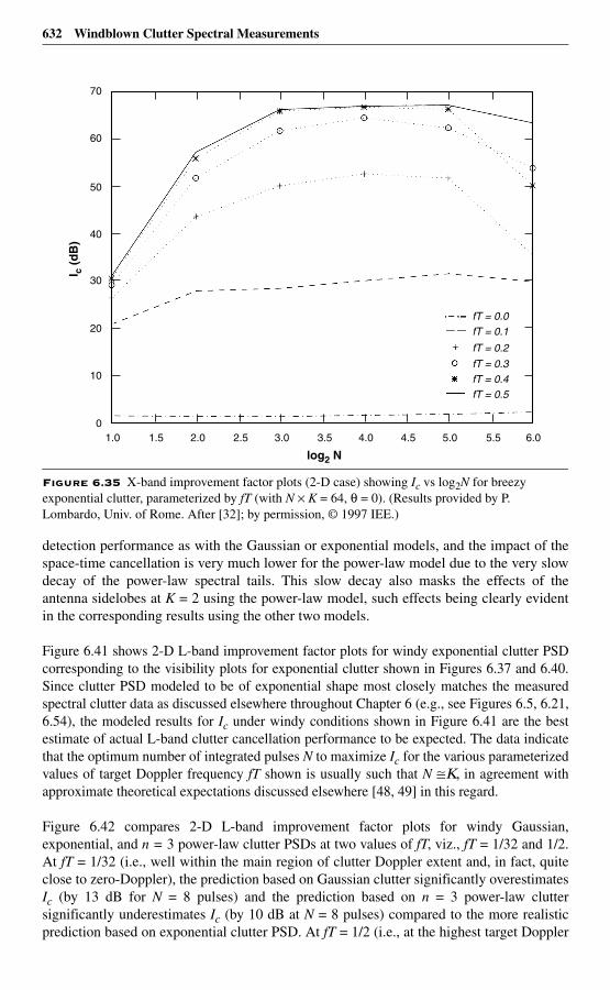
632 Windblown Clutter Spectral Measurements

detection performance as with the Gaussian or exponential models, and the impact of thespace-time cancellation is very much lower for the power-law model due to the very slowdecay of the power-law spectral tails. This slow decay also masks the effects of theantenna sidelobes at K = 2 using the power-law model, such effects being clearly evidentin the corresponding results using the other two models.

Figure 6.41 shows 2-D L-band improvement factor plots for windy exponential clutter PSDcorresponding to the visibility plots for exponential clutter shown in Figures 6.37 and 6.40.Since clutter PSD modeled to be of exponential shape most closely matches the measuredspectral clutter data as discussed elsewhere throughout Chapter 6 (e.g., see Figures 6.5, 6.21,6.54), the modeled results for Ic under windy conditions shown in Figure 6.41 are the bestestimate of actual L-band clutter cancellation performance to be expected. The data indicatethat the optimum number of integrated pulses N to maximize Ic for the various parameterizedvalues of target Doppler frequency fT shown is usually such that N ≅Κ, in agreement withapproximate theoretical expectations discussed elsewhere [48, 49] in this regard.

Figure 6.42 compares 2-D L-band improvement factor plots for windy Gaussian,exponential, and n = 3 power-law clutter PSDs at two values of fT, viz., fT = 1/32 and 1/2.At fT = 1/32 (i.e., well within the main region of clutter Doppler extent and, in fact, quiteclose to zero-Doppler), the prediction based on Gaussian clutter significantly overestimatesIc (by 13 dB for N = 8 pulses) and the prediction based on n = 3 power-law cluttersignificantly underestimates Ic (by 10 dB at N = 8 pulses) compared to the more realisticprediction based on exponential clutter PSD. At fT = 1/2 (i.e., at the highest target Doppler

Figure 6.35 X-band improvement factor plots (2-D case) showing Ic vs log2N for breezy exponential clutter, parameterized by fT (with N × K = 64, θ = 0). (Results provided by P. Lombardo, Univ. of Rome. After [32]; by permission, © 1997 IEE.)

I c (

dB

)

log2 N

1.51.0 2.0 2.5 3.0 3.5 4.0 4.5 5.0 5.5 6.0

70

60

50

40

30

20

10

0

fT = 0.0fT = 0.1

fT = 0.2

fT = 0.3fT = 0.4fT = 0.5

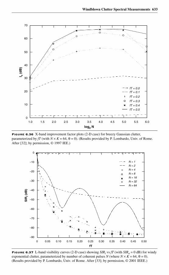
Windblown Clutter Spectral Measurements 633

Figure 6.36 X-band improvement factor plots (2-D case) for breezy Gaussian clutter, parameterized by fT (with N × K = 64, θ = 0). (Results provided by P. Lombardo, Univ. of Rome. After [32]; by permission, © 1997 IEE.)

Figure 6.37 L-band visibility curves (2-D case) showing SIRi vs fT (with SIRo = 0 dB) for windy exponential clutter, parameterized by number of coherent pulses N (where N × K = 64, θ = 0). (Results provided by P. Lombardo, Univ. of Rome. After [33]; by permission, © 2001 IEEE.)

I c (

dB

)

log2 N

1.51.0 2.0 2.5 3.0 3.5 4.0 4.5 5.0 5.5 6.0

70

60

50

40

30

20

10

0

fT = 0.0fT = 0.1

fT = 0.2

fT = 0.3

fT = 0.4

fT = 0.5

SIR

i (d

B)

fT

0.050 0.10 0.15 0.20 0.25 0.30 0.35 0.40 0.45 0.50

0

–10

–20

–30

–40

–50

–60

–70

–80

–90

N = 2

N = 1

N = 4

N = 8

N = 16

N = 32

N = 64

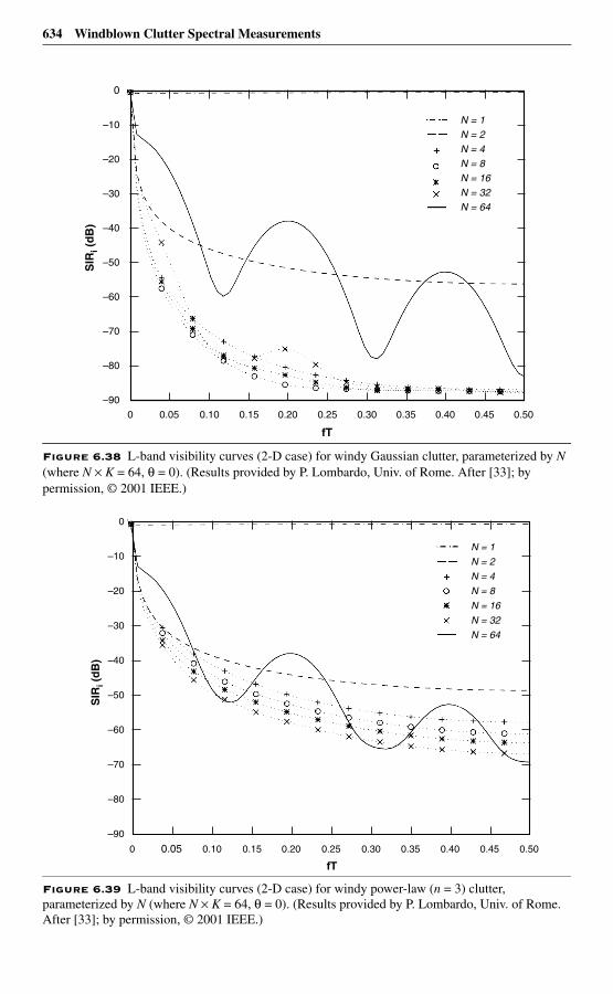
634 Windblown Clutter Spectral Measurements

Figure 6.38 L-band visibility curves (2-D case) for windy Gaussian clutter, parameterized by N (where N × K = 64, θ = 0). (Results provided by P. Lombardo, Univ. of Rome. After [33]; by permission, © 2001 IEEE.)

Figure 6.39 L-band visibility curves (2-D case) for windy power-law (n = 3) clutter, parameterized by N (where N × K = 64, θ = 0). (Results provided by P. Lombardo, Univ. of Rome. After [33]; by permission, © 2001 IEEE.)

SIR

i (d

B)

fT

0.050 0.10 0.15 0.20 0.25 0.30 0.35 0.40 0.45 0.50

0

–10

–20

–30

–40

–50

–60

–70

–80

–90

N = 2N = 1

N = 4N = 8N = 16N = 32N = 64

SIR

i (d

B)

fT

0.050 0.10 0.15 0.20 0.25 0.30 0.35 0.40 0.45 0.50

0

–10

–20

–30

–40

–50

–60

–70

–80

–90

N = 2

N = 1

N = 4

N = 8

N = 16

N = 32

N = 64

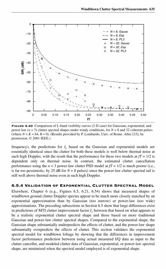
Windblown Clutter Spectral Measurements 635

frequency), the predictions for Ic based on the Gaussian and exponential models areessentially identical since the clutter for both these models is well below thermal noise atsuch high Doppler, with the result that the performance for these two models at fT = 1/2 isdependent only on thermal noise. In contrast, the estimated clutter cancellationperformance using the n = 3 power-law clutter PSD model at fT = 1/2 is much poorer (i.e.,is far too pessimistic, by 25 dB for N = 8 pulses) since the power-law clutter spectral tail isstill well above thermal noise even at such high Doppler.

6.5.4 Validation of Exponential Clutter Spectral ModelElsewhere, Chapter 6 (e.g., Figures 6.5, 6.21, 6.54) shows that measured shapes ofwindblown ground clutter Doppler spectra appear to be much more closely matched by anexponential approximation than by Gaussian (too narrow) or power-law (too wide)approximations. The preceding subsections in Section 6.5 show that large differences existin predictions of MTI clutter improvement factor Ic between that based on what appears tobe a realistic exponential clutter spectral shape and those based on more traditionalGaussian and power-law clutter spectral shapes. Compared to the exponential shape, theGaussian shape substantially underpredicts the effects of clutter, and the power-law shapesubstantially overpredicts the effects of clutter. This section validates the exponentialspectral model for windblown foliage by showing that the differences in improvementfactor performance prediction between using actual measured I/Q data as input to theclutter canceller, and modeled clutter data of Gaussian, exponential, or power-law spectralshape, are minimized when the spectral model employed is of exponential shape.

Figure 6.40 Comparison of L-band visibility curves (2-D case) for Gaussian, exponential, and power law (n = 3) clutter spectral shapes under windy conditions, for N = 8 and 32 coherent pulses (where N × K = 64, θ = 0). (Results provided by P. Lombardo, Univ. of Rome. After [33]; by permission, © 2001 IEEE.)

SIR

i (d

B)

fT0.050 0.10 0.15 0.20 0.25 0.30 0.35 0.40 0.45 0.50

0

–10

–20

–30

–40

–50

–60

–70

–80

–90

N = 8, ExpN = 8, Gauss

N = 8, PL3N = 32, GaussN = 32, ExpN = 32, PL3

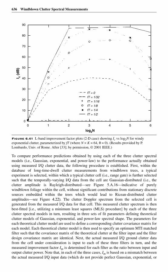
636 Windblown Clutter Spectral Measurements

To compare performance predictions obtained by using each of the three clutter spectralmodels (i.e., Gaussian, exponential, and power-law) to the performance actually obtainedusing measured I/Q clutter data, the following procedure is established. First, within thedatabase of long-time-dwell clutter measurements from windblown trees, a typicalexperiment is selected, within which a typical clutter cell (i.e., range gate) is further selectedsuch that the temporally-varying I/Q data from the cell are Gaussian-distributed (i.e., theclutter amplitude is Rayleigh-distributed—see Figure 5.A.16—indicative of purelywindblown foliage within the cell, without significant contributions from stationary discretesources embedded within the trees which would lead to Ricean-distributed clutteramplitudes—see Figure 4.22). The clutter Doppler spectrum from the selected cell isgenerated from the measured I/Q data for that cell. This measured clutter spectrum is thenbest-fitted [i.e., utilizing a minimum least squares (MLS) procedure] by each of the threeclutter spectral models in turn, resulting in three sets of fit parameters defining theoreticalclutter models of Gaussian, exponential, and power-law spectral shape. The parameters foreach theoretical clutter model are used to define a corresponding clutter covariance matrix foreach model. Each theoretical clutter model is then used to specify an optimum MTI matchedfilter such that the covariance matrix of the theoretical clutter at the filter input and the filterdesign covariance matrix are identical. Next, the actual measured I/Q ground clutter datafrom the cell under consideration is input to each of these three filters in turn, and themeasured improvement factor Im is determined for each filter as the ratio between input andoutput clutter power. Note that, in each of the three cases, Im is based on a mismatch betweenthe actual measured I/Q input data (which do not provide perfect Gaussian, exponential, or

Figure 6.41 L-band improvement factor plots (2-D case) showing Ic vs log2N for windy exponential clutter, parameterized by fT (where N × K = 64, θ = 0). (Results provided by P. Lombardo, Univ. of Rome. After [33]; by permission, © 2001 IEEE.)

I c (

dB

)

log2N

10 2 3 4 5 6

90

80

70

60

50

40

30

20

10

0

fT = 1/32fT = 0

fT = 1/16fT = 1/8fT = 1/4fT = 1/2

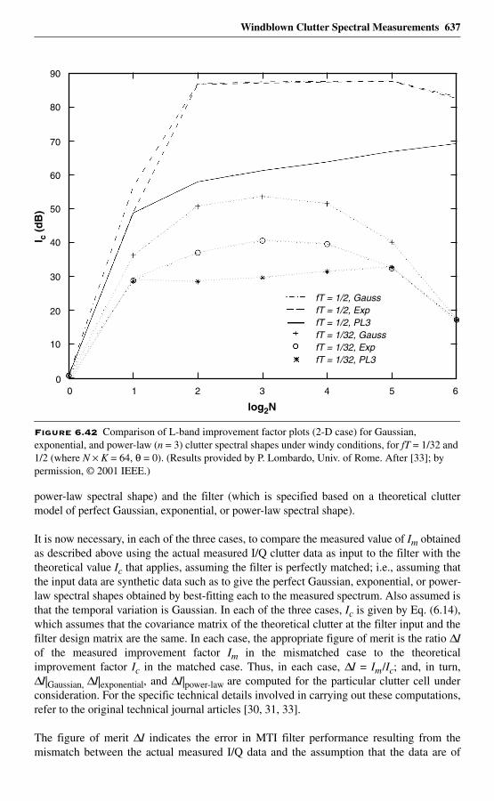
Windblown Clutter Spectral Measurements 637

power-law spectral shape) and the filter (which is specified based on a theoretical cluttermodel of perfect Gaussian, exponential, or power-law spectral shape).

It is now necessary, in each of the three cases, to compare the measured value of Im obtainedas described above using the actual measured I/Q clutter data as input to the filter with thetheoretical value Ic that applies, assuming the filter is perfectly matched; i.e., assuming thatthe input data are synthetic data such as to give the perfect Gaussian, exponential, or power-law spectral shapes obtained by best-fitting each to the measured spectrum. Also assumed isthat the temporal variation is Gaussian. In each of the three cases, Ic is given by Eq. (6.14),which assumes that the covariance matrix of the theoretical clutter at the filter input and thefilter design matrix are the same. In each case, the appropriate figure of merit is the ratio ∆Iof the measured improvement factor Im in the mismatched case to the theoreticalimprovement factor Ic in the matched case. Thus, in each case, ∆I = Im/Ic; and, in turn,∆I|Gaussian, ∆I|exponential, and ∆I|power-law are computed for the particular clutter cell underconsideration. For the specific technical details involved in carrying out these computations,refer to the original technical journal articles [30, 31, 33].

The figure of merit ∆I indicates the error in MTI filter performance resulting from themismatch between the actual measured I/Q data and the assumption that the data are of

Figure 6.42 Comparison of L-band improvement factor plots (2-D case) for Gaussian, exponential, and power-law (n = 3) clutter spectral shapes under windy conditions, for fT = 1/32 and 1/2 (where N × K = 64, θ = 0). (Results provided by P. Lombardo, Univ. of Rome. After [33]; by permission, © 2001 IEEE.)

I c (

dB

)

log2N

10 2 3 4 5 6

90

80

70

60

50

40

30

20

10

0

fT = 1/2, ExpfT = 1/2, Gauss

fT = 1/2, PL3fT = 1/32, GaussfT = 1/32, ExpfT = 1/32, PL3

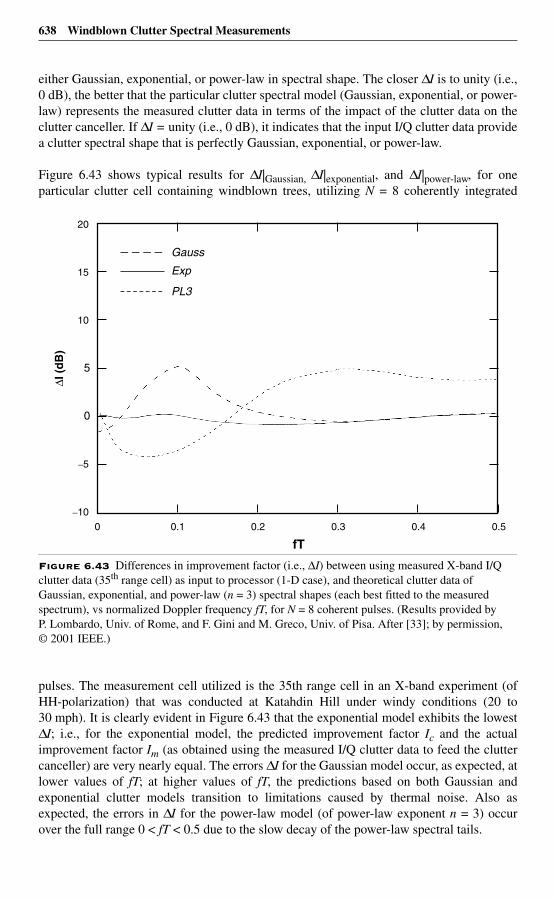
638 Windblown Clutter Spectral Measurements

either Gaussian, exponential, or power-law in spectral shape. The closer ∆I is to unity (i.e.,0 dB), the better that the particular clutter spectral model (Gaussian, exponential, or power-law) represents the measured clutter data in terms of the impact of the clutter data on theclutter canceller. If ∆I = unity (i.e., 0 dB), it indicates that the input I/Q clutter data providea clutter spectral shape that is perfectly Gaussian, exponential, or power-law.

Figure 6.43 shows typical results for ∆I|Gaussian, ∆I|exponential, and ∆I|power-law, for oneparticular clutter cell containing windblown trees, utilizing N = 8 coherently integrated

pulses. The measurement cell utilized is the 35th range cell in an X-band experiment (ofHH-polarization) that was conducted at Katahdin Hill under windy conditions (20 to30 mph). It is clearly evident in Figure 6.43 that the exponential model exhibits the lowest∆I; i.e., for the exponential model, the predicted improvement factor Ic and the actualimprovement factor Im (as obtained using the measured I/Q clutter data to feed the cluttercanceller) are very nearly equal. The errors ∆I for the Gaussian model occur, as expected, atlower values of fT; at higher values of fT, the predictions based on both Gaussian andexponential clutter models transition to limitations caused by thermal noise. Also asexpected, the errors in ∆I for the power-law model (of power-law exponent n = 3) occurover the full range 0 < fT < 0.5 due to the slow decay of the power-law spectral tails.

Figure 6.43 Differences in improvement factor (i.e., ∆I) between using measured X-band I/Q clutter data (35th range cell) as input to processor (1-D case), and theoretical clutter data of Gaussian, exponential, and power-law (n = 3) spectral shapes (each best fitted to the measured spectrum), vs normalized Doppler frequency fT, for N = 8 coherent pulses. (Results provided by P. Lombardo, Univ. of Rome, and F. Gini and M. Greco, Univ. of Pisa. After [33]; by permission, © 2001 IEEE.)

∆I (

dB

)

fT0.10 0.2 0.3 0.4 0.5

20

15

10

5

0

–5

–10

Exp

Gauss

PL3

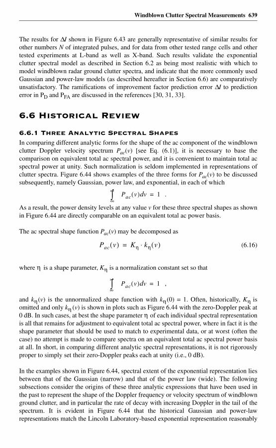
Windblown Clutter Spectral Measurements 639

The results for ∆I shown in Figure 6.43 are generally representative of similar results forother numbers N of integrated pulses, and for data from other tested range cells and othertested experiments at L-band as well as X-band. Such results validate the exponentialclutter spectral model as described in Section 6.2 as being most realistic with which tomodel windblown radar ground clutter spectra, and indicate that the more commonly usedGaussian and power-law models (as described hereafter in Section 6.6) are comparativelyunsatisfactory. The ramifications of improvement factor prediction error ∆I to predictionerror in PD and PFA are discussed in the references [30, 31, 33].

6.6 Historical Review

6.6.1 Three Analytic Spectral ShapesIn comparing different analytic forms for the shape of the ac component of the windblownclutter Doppler velocity spectrum Pac(v) [see Eq. (6.1)], it is necessary to base thecomparison on equivalent total ac spectral power, and it is convenient to maintain total acspectral power at unity. Such normalization is seldom implemented in representations ofclutter spectra. Figure 6.44 shows examples of the three forms for Pac(v) to be discussedsubsequently, namely Gaussian, power law, and exponential, in each of which

.

As a result, the power density levels at any value v for these three spectral shapes as shownin Figure 6.44 are directly comparable on an equivalent total ac power basis.

The ac spectral shape function Pac(v) may be decomposed as

(6.16)

where η is a shape parameter, Kη is a normalization constant set so that

,

and kη(v) is the unnormalized shape function with kη(0) = 1. Often, historically, Kη isomitted and only kη (v) is shown in plots such as Figure 6.44 with the zero-Doppler peak at0 dB. In such cases, at best the shape parameter η of each individual spectral representationis all that remains for adjustment to equivalent total ac spectral power, where in fact it is theshape parameter that should be used to match to experimental data, or at worst (often thecase) no attempt is made to compare spectra on an equivalent total ac spectral power basisat all. In short, in comparing different analytic spectral representations, it is not rigorouslyproper to simply set their zero-Doppler peaks each at unity (i.e., 0 dB).

In the examples shown in Figure 6.44, spectral extent of the exponential representation liesbetween that of the Gaussian (narrow) and that of the power law (wide). The followingsubsections consider the origins of these three analytic expressions that have been used inthe past to represent the shape of the Doppler frequency or velocity spectrum of windblownground clutter, and in particular the rate of decay with increasing Doppler in the tail of thespectrum. It is evident in Figure 6.44 that the historical Gaussian and power-lawrepresentations match the Lincoln Laboratory-based exponential representation reasonably

Pac v( ) vd∞–

∞∫ 1=

Pac v( ) Kη kη v( )⋅=

Pac v( ) vd∞

∞∫ 1=

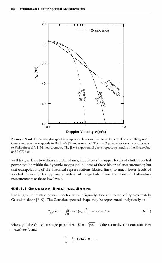
640 Windblown Clutter Spectral Measurements

well (i.e., at least to within an order of magnitude) over the upper levels of clutter spectralpower that lie within the dynamic ranges (solid lines) of these historical measurements; butthat extrapolations of the historical representations (dotted lines) to much lower levels ofspectral power differ by many orders of magnitude from the Lincoln Laboratorymeasurements at these low levels.

6.6.1.1 Gaussian Spectral Shape

Radar ground clutter power spectra were originally thought to be of approximatelyGaussian shape [6–9]. The Gaussian spectral shape may be represented analytically as

, –∞ < v < ∞ (6.17)

where g is the Gaussian shape parameter, is the normalization constant, k(v)= exp(–gv2), and

.

Figure 6.44 Three analytic spectral shapes, each normalized to unit spectral power. The g = 20 Gaussian curve corresponds to Barlow’s [7] measurement. The n = 3 power-law curve corresponds to Fishbein et al.’s [10] measurement. The β = 6 exponential curve represents much of the Phase One and LCE data.

20

0

–20

–40

–60

–800.1 1 10

Pac

(d

B)

Doppler Velocity v (m/s)

Gaussian

Power Law

n = 3, vc = 0.107

Exponential

= 6

Extrapolation

g = 20

Pac v( ) gπ--- gv

2–( )exp⋅=

K g π⁄=

Pac v( ) vd∞–

∞∫ 1=

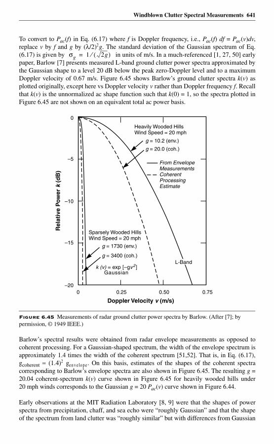
Windblown Clutter Spectral Measurements 641

To convert to Pac(f) in Eq. (6.17) where f is Doppler frequency, i.e., Pac(f) df = Pac(v)dv,replace v by f and g by (λ/2)2g. The standard deviation of the Gaussian spectrum of Eq.(6.17) is given by in units of m/s. In a much-referenced [1, 27, 50] earlypaper, Barlow [7] presents measured L-band ground clutter power spectra approximated bythe Gaussian shape to a level 20 dB below the peak zero-Doppler level and to a maximumDoppler velocity of 0.67 m/s. Figure 6.45 shows Barlow’s ground clutter spectra k(v) asplotted originally, except here vs Doppler velocity v rather than Doppler frequency f. Recallthat k(v) is the unnormalized ac shape function such that k(0) = 1, so the spectra plotted inFigure 6.45 are not shown on an equivalent total ac power basis.

Barlow’s spectral results were obtained from radar envelope measurements as opposed tocoherent processing. For a Gaussian-shaped spectrum, the width of the envelope spectrum isapproximately 1.4 times the width of the coherent spectrum [51,52]. That is, in Eq. (6.17),gcoherent ≈ (1.4)2 gen v e lo p e. On this basis, estimates of the shapes of the coherent spectracorresponding to Barlow’s envelope spectra are also shown in Figure 6.45. The resulting g =20.04 coherent-spectrum k(v) curve shown in Figure 6.45 for heavily wooded hills under20 mph winds corresponds to the Gaussian g = 20 Pac(v) curve shown in Figure 6.44.

Early observations at the MIT Radiation Laboratory [8, 9] were that the shapes of powerspectra from precipitation, chaff, and sea echo were “roughly Gaussian” and that the shapeof the spectrum from land clutter was “roughly similar” but with differences from Gaussian

Figure 6.45 Measurements of radar ground clutter power spectra by Barlow. (After [7]; by permission, © 1949 IEEE.)

σg 1 2g( )⁄=

0

–5

–10

–15

–200 0.25 0.50 0.75

Doppler Velocity v (m/s)

Rel

ativ

e P

ow

er k

(d

B)

g = 3400 (coh.)

g = 1730 (env.)

From EnvelopeMeasurementsCoherentProcessingEstimate

Heavily Wooded HillsWind Speed = 20 mph

g = 20.0 (coh.)

g = 10.2 (env.)

Sparsely Wooded HillsWind Speed = 20 mph

k (v) = exp [–gv2]L-Band

Gaussian

642 Windblown Clutter Spectral Measurements

shape “somewhat more pronounced.” The explanation for clutter spectra of approximatelyGaussian shape is loosely based on the idea that windblown vegetation consistsfundamentally of a random array of elemental moving scatterers, each with a constanttranslational drift velocity. If the distribution of radial velocities of such a group ofscatterers were approximately Gaussian, they would generate an approximately Gaussian-shaped power spectrum. However, consider if the motion of the scatterers also were toinclude an oscillatory component to represent branches and leaves blowing back and forthin the wind. It is well known [53] that simple harmonic angle modulation (frequency orphase) generates an infinite series of sidebands so that an array of oscillating scattererswould be expected to generate a wider spectrum than an array of scatterers each with only aconstant drift velocity.

Indeed, in 1967 Wong, Reed, and Kaprielian [29] provided an analysis of the scatteredsignal and power spectrum from an array of scatterers, each with random rotational(oscillatory) motion as well as a constant random drift velocity. Under assumptions ofGaussianly distributed drift and rotational velocities, Wong et al. [29] showed that thepower spectrum of the scattered signal is the sum of six components. Li [19] subsequentlyprovided further interpretation of these six components, as follows. If scatterer rotation isabsent, the Wong et al. expression for the clutter spectrum degenerates to Barlow’s simpleGaussian expression, i.e., Eq. (6.17). However, with scatterer rotation present, fiveadditional Gaussian components arise, all of which decay more slowly and all but one ofwhich are offset from zero-Doppler (by ± 2 and ± 4 times the rotational velocity). As aresult, these five additional Gaussian terms that come into play with scatterer rotation act to“spread” the spectrum beyond that of the simple Gaussian of Eq. (6.17). Narayanan et al.[42] returned to Wong’s formulation of offset Gaussians in modeling some later-acquiredX-band windblown clutter spectral measurements.

In 1965, two years before the publication of the Wong et al. paper [29], Bass, Bliokh, andFuks [54] also provided a theoretical study of scattering from oscillating reradiators tomodel scattering from windblown vegetation. In the Bass et al. paper, the reradiators weremodeled to be decaying oscillators randomly positioned on a planar surface. In theiranalysis, Bass et al. showed that the power spectrum of the scattered radiation from theoscillating reradiators consists of a doubly infinite sum of offset Gaussian functions, butwhen the reradiators do not oscillate, the power spectrum simplifies to a sum of simplenon-offset Gaussians. It is evident that these results have some degree of similarity withthose of Wong et al. [29] in that both represent the power spectrum from a group ofoscillating random scatterers as sums of Gaussians, the peaks of which are offset fromzero-Doppler and for which the offsets collapse in the absence of oscillation.

Some years following both the Wong et al. [29] and the Bass et al. papers [54], Rosenbaumand Bowles [55] derived theoretical expressions for windblown clutter spectra based on aphysical model in which the backscattering was associated with random permittivityfluctuations superimposed on a lossy background slab. Again with overtones of similarityto both the Wong et al. and the Bass et al. analyses, Rosenbaum and Bowles modeledscatterer motion two ways, first, as a Gaussian process, and second, assuming scatterermotion to be quasi-harmonic, so that the scatterers behave as decaying simple-harmonicoscillators. It has been observed that the Rosenbaum and Bowles spectral results “are . . .too complex for radar engineers to use in design practice” [19].

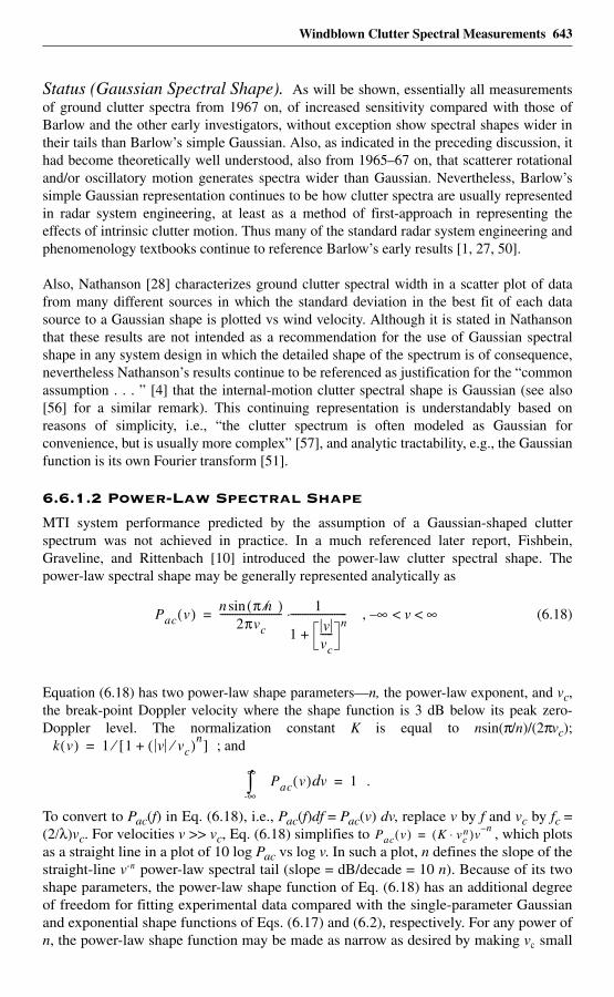
Windblown Clutter Spectral Measurements 643

Status (Gaussian Spectral Shape). As will be shown, essentially all measurementsof ground clutter spectra from 1967 on, of increased sensitivity compared with those ofBarlow and the other early investigators, without exception show spectral shapes wider intheir tails than Barlow’s simple Gaussian. Also, as indicated in the preceding discussion, ithad become theoretically well understood, also from 1965–67 on, that scatterer rotationaland/or oscillatory motion generates spectra wider than Gaussian. Nevertheless, Barlow’ssimple Gaussian representation continues to be how clutter spectra are usually representedin radar system engineering, at least as a method of first-approach in representing theeffects of intrinsic clutter motion. Thus many of the standard radar system engineering andphenomenology textbooks continue to reference Barlow’s early results [1, 27, 50].

Also, Nathanson [28] characterizes ground clutter spectral width in a scatter plot of datafrom many different sources in which the standard deviation in the best fit of each datasource to a Gaussian shape is plotted vs wind velocity. Although it is stated in Nathansonthat these results are not intended as a recommendation for the use of Gaussian spectralshape in any system design in which the detailed shape of the spectrum is of consequence,nevertheless Nathanson’s results continue to be referenced as justification for the “commonassumption . . . ” [4] that the internal-motion clutter spectral shape is Gaussian (see also[56] for a similar remark). This continuing representation is understandably based onreasons of simplicity, i.e., “the clutter spectrum is often modeled as Gaussian forconvenience, but is usually more complex” [57], and analytic tractability, e.g., the Gaussianfunction is its own Fourier transform [51].

6.6.1.2 Power-Law Spectral Shape

MTI system performance predicted by the assumption of a Gaussian-shaped clutterspectrum was not achieved in practice. In a much referenced later report, Fishbein,Graveline, and Rittenbach [10] introduced the power-law clutter spectral shape. Thepower-law spectral shape may be generally represented analytically as

, –∞ < v < ∞ (6.18)

Equation (6.18) has two power-law shape parameters—n, the power-law exponent, and vc,the break-point Doppler velocity where the shape function is 3 dB below its peak zero-Doppler level. The normalization constant K is equal to nsin(π/n)/(2πvc);

; and

.

To convert to Pac(f) in Eq. (6.18), i.e., Pac(f)df = Pac(v) dv, replace v by f and vc by fc =(2/λ)vc. For velocities v >> vc, Eq. (6.18) simplifies to , which plotsas a straight line in a plot of 10 log Pac vs log v. In such a plot, n defines the slope of thestraight-line v-n power-law spectral tail (slope = dB/decade = 10 n). Because of its twoshape parameters, the power-law shape function of Eq. (6.18) has an additional degreeof freedom for fitting experimental data compared with the single-parameter Gaussianand exponential shape functions of Eqs. (6.17) and (6.2), respectively. For any power ofn, the power-law shape function may be made as narrow as desired by making vc small

Pac v( ) n π n⁄( )sin2πvc

------------------------- 1

1vvc-----

n+

-----------------------⋅=

k v( ) 1 1 v vc⁄( )n+[ ]⁄=

Pac v( ) vd∞–

∞∫ 1=

Pac v( ) K vcn⋅( )v

n–=

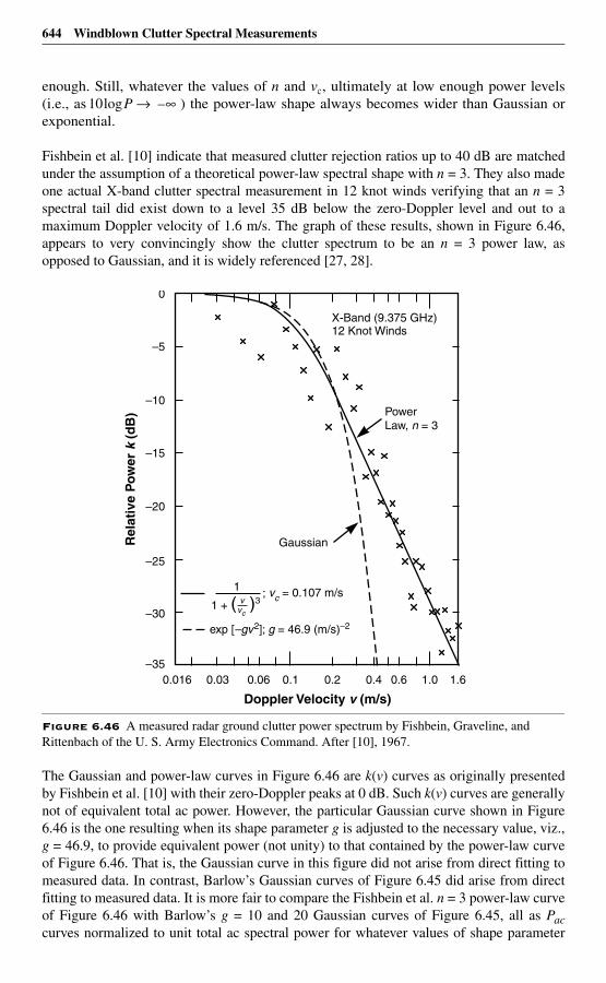
644 Windblown Clutter Spectral Measurements

enough. Still, whatever the values of n and vc, ultimately at low enough power levels(i.e., as ) the power-law shape always becomes wider than Gaussian orexponential.

Fishbein et al. [10] indicate that measured clutter rejection ratios up to 40 dB are matchedunder the assumption of a theoretical power-law spectral shape with n = 3. They also madeone actual X-band clutter spectral measurement in 12 knot winds verifying that an n = 3spectral tail did exist down to a level 35 dB below the zero-Doppler level and out to amaximum Doppler velocity of 1.6 m/s. The graph of these results, shown in Figure 6.46,appears to very convincingly show the clutter spectrum to be an n = 3 power law, asopposed to Gaussian, and it is widely referenced [27, 28].

The Gaussian and power-law curves in Figure 6.46 are k(v) curves as originally presentedby Fishbein et al. [10] with their zero-Doppler peaks at 0 dB. Such k(v) curves are generallynot of equivalent total ac power. However, the particular Gaussian curve shown in Figure6.46 is the one resulting when its shape parameter g is adjusted to the necessary value, viz.,g = 46.9, to provide equivalent power (not unity) to that contained by the power-law curveof Figure 6.46. That is, the Gaussian curve in this figure did not arise from direct fitting tomeasured data. In contrast, Barlow’s Gaussian curves of Figure 6.45 did arise from directfitting to measured data. It is more fair to compare the Fishbein et al. n = 3 power-law curveof Figure 6.46 with Barlow’s g = 10 and 20 Gaussian curves of Figure 6.45, all as Paccurves normalized to unit total ac spectral power for whatever values of shape parameter

Figure 6.46 A measured radar ground clutter power spectrum by Fishbein, Graveline, and Rittenbach of the U. S. Army Electronics Command. After [10], 1967.

10 P ∞–→log

–30

Doppler Velocity v (m/s)

Rel

ativ

e P

ow

er k

(d

B)

–20

–10

0

–35

–25

–15

–5

0.03 0.06 0.1 0.2 0.4 1.0 1.6

PowerLaw, n = 3

X-Band (9.375 GHz)12 Knot Winds

1

1 + ( )3vc

v; vc = 0.107 m/s

exp [–gv2]; g = 46.9 (m/s)–2

Gaussian

0.016 0.6

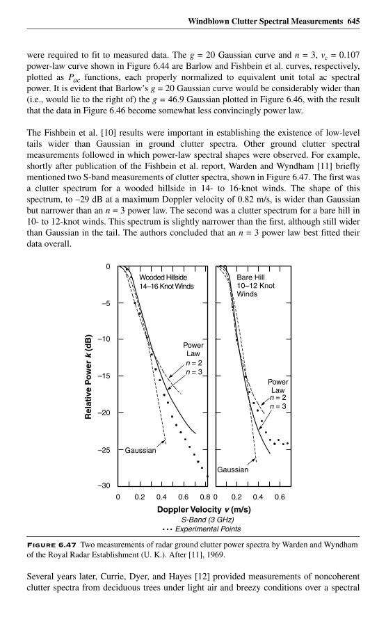
Windblown Clutter Spectral Measurements 645

were required to fit to measured data. The g = 20 Gaussian curve and n = 3, vc = 0.107power-law curve shown in Figure 6.44 are Barlow and Fishbein et al. curves, respectively,plotted as Pac functions, each properly normalized to equivalent unit total ac spectralpower. It is evident that Barlow’s g = 20 Gaussian curve would be considerably wider than(i.e., would lie to the right of) the g = 46.9 Gaussian plotted in Figure 6.46, with the resultthat the data in Figure 6.46 become somewhat less convincingly power law.

The Fishbein et al. [10] results were important in establishing the existence of low-leveltails wider than Gaussian in ground clutter spectra. Other ground clutter spectralmeasurements followed in which power-law spectral shapes were observed. For example,shortly after publication of the Fishbein et al. report, Warden and Wyndham [11] brieflymentioned two S-band measurements of clutter spectra, shown in Figure 6.47. The first wasa clutter spectrum for a wooded hillside in 14- to 16-knot winds. The shape of thisspectrum, to –29 dB at a maximum Doppler velocity of 0.82 m/s, is wider than Gaussianbut narrower than an n = 3 power law. The second was a clutter spectrum for a bare hill in10- to 12-knot winds. This spectrum is slightly narrower than the first, although still widerthan Gaussian in the tail. The authors concluded that an n = 3 power law best fitted theirdata overall.

Several years later, Currie, Dyer, and Hayes [12] provided measurements of noncoherentclutter spectra from deciduous trees under light air and breezy conditions over a spectral

Figure 6.47 Two measurements of radar ground clutter power spectra by Warden and Wyndham of the Royal Radar Establishment (U. K.). After [11], 1969.

–30

Doppler Velocity v (m/s)

Rel

ativ

e P

ow

er k

(d

B)

–20

–10

0

–25

–15

–5

0

Wooded Hillside14–16 Knot Winds

0.2 0.4 0.6 0.8

n = 2n = 3

Gaussian

0 0.2 0.4 0.6

n = 2n = 3

Bare Hill10–12 KnotWinds

Gaussian

S-Band (3 GHz) Experimental Points

PowerLaw

PowerLaw

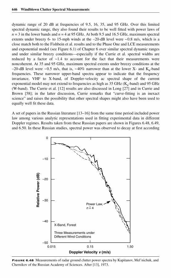
646 Windblown Clutter Spectral Measurements

dynamic range of 20 dB at frequencies of 9.5, 16, 35, and 95 GHz. Over this limitedspectral dynamic range, they also found their results to be well fitted with power laws ofn = 3 in the lower bands and n = 4 at 95 GHz. At both 9.5 and 16.5 GHz, maximum spectralextents under breezy 6- to 15-mph winds at the –20-dB level were ~0.8 m/s, which is aclose match both to the Fishbein et al. results and to the Phase One and LCE measurementsand exponential model (see Figure 6.1) of Chapter 6 over similar spectral dynamic rangesand under similar breezy conditions—especially if the Currie et al. spectral widths arereduced by a factor of ~1.4 to account for the fact that their measurements werenoncoherent. At 35 and 95 GHz, maximum spectral extents under breezy conditions at the–20-dB level were ~0.5 m/s, that is, ~40% narrower than at the lower X- and Ku-bandfrequencies. These narrower upper-band spectra appear to indicate that the frequencyinvariance, VHF to X-band, of Doppler-velocity ac spectral shape of the currentexponential model may not extend to frequencies as high as 35 GHz (Ka-band) and 95 GHz(W-band). The Currie et al. [12] results are also discussed in Long [27] and in Currie andBrown [58]; in the latter discussion, Currie remarks that “curve-fitting is an inexactscience” and raises the possibility that other spectral shapes might also have been used toequally well fit these data.

A set of papers in the Russian literature [13–16] from the same time period included powerlaw among various analytic representations used in fitting experimental data in differentDoppler regimes. Results taken from these Russian papers are shown in Figures 6.48, 6.49,and 6.50. In these Russian studies, spectral power was observed to decay at first according

Figure 6.48 Measurements of radar ground clutter power spectra by Kapitanov, Mel’nichuk, and Chernikov of the Russian Academy of Sciences. After [13], 1973.

0.015 1.50–50

–40

–30

–10

0

Doppler Velocity v (m/s)

Rel

ativ

e P

ow

er (

dB

)

–20

0.15

X-Band, Forest

Three Measurements underDifferent Wind Conditions

Power Law,n = 4 ~

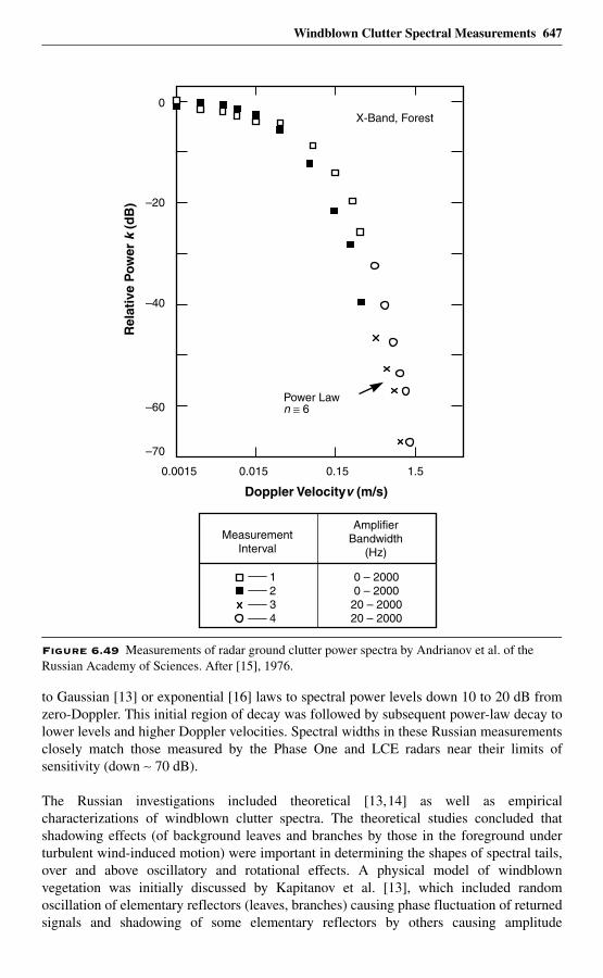
Windblown Clutter Spectral Measurements 647

to Gaussian [13] or exponential [16] laws to spectral power levels down 10 to 20 dB fromzero-Doppler. This initial region of decay was followed by subsequent power-law decay tolower levels and higher Doppler velocities. Spectral widths in these Russian measurementsclosely match those measured by the Phase One and LCE radars near their limits ofsensitivity (down ∼ 70 dB).

The Russian investigations included theoretical [13,14] as well as empiricalcharacterizations of windblown clutter spectra. The theoretical studies concluded thatshadowing effects (of background leaves and branches by those in the foreground underturbulent wind-induced motion) were important in determining the shapes of spectral tails,over and above oscillatory and rotational effects. A physical model of windblownvegetation was initially discussed by Kapitanov et al. [13], which included randomoscillation of elementary reflectors (leaves, branches) causing phase fluctuation of returnedsignals and shadowing of some elementary reflectors by others causing amplitude

Figure 6.49 Measurements of radar ground clutter power spectra by Andrianov et al. of the Russian Academy of Sciences. After [15], 1976.

0.0015 0.015 0.15 1.5

–70

–60

–40

–20

0

Doppler Velocityv (m/s)

Rel

ativ

e P

ow

er k

(d

B)

MeasurementInterval

AmplifierBandwidth

(Hz)

1234

0 – 20000 – 200020 – 200020 – 2000

X-Band, Forest

n ≅ 6 Power Law

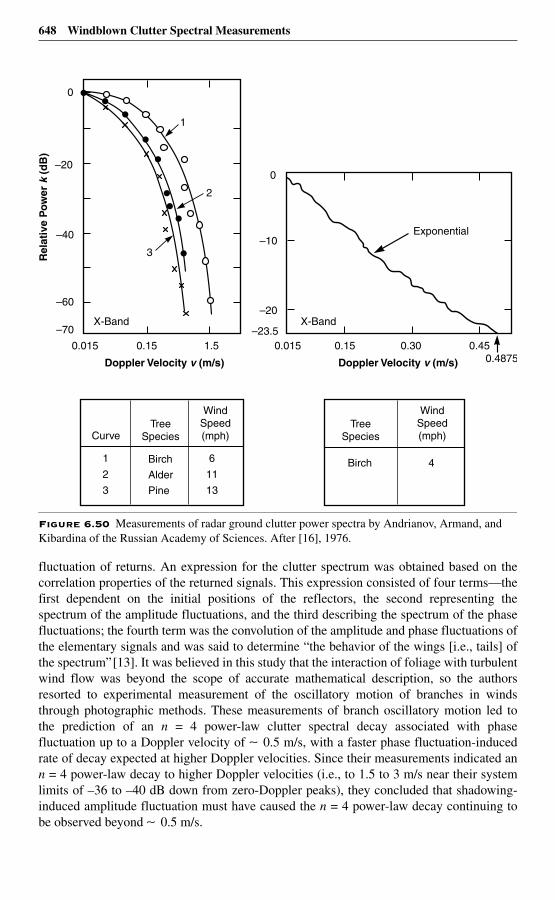
648 Windblown Clutter Spectral Measurements

fluctuation of returns. An expression for the clutter spectrum was obtained based on thecorrelation properties of the returned signals. This expression consisted of four terms—thefirst dependent on the initial positions of the reflectors, the second representing thespectrum of the amplitude fluctuations, and the third describing the spectrum of the phasefluctuations; the fourth term was the convolution of the amplitude and phase fluctuations ofthe elementary signals and was said to determine “the behavior of the wings [i.e., tails] ofthe spectrum”[13]. It was believed in this study that the interaction of foliage with turbulentwind flow was beyond the scope of accurate mathematical description, so the authorsresorted to experimental measurement of the oscillatory motion of branches in windsthrough photographic methods. These measurements of branch oscillatory motion led tothe prediction of an n = 4 power-law clutter spectral decay associated with phasefluctuation up to a Doppler velocity of ∼ 0.5 m/s, with a faster phase fluctuation-inducedrate of decay expected at higher Doppler velocities. Since their measurements indicated ann = 4 power-law decay to higher Doppler velocities (i.e., to 1.5 to 3 m/s near their systemlimits of –36 to –40 dB down from zero-Doppler peaks), they concluded that shadowing-induced amplitude fluctuation must have caused the n = 4 power-law decay continuing tobe observed beyond ∼ 0.5 m/s.

Figure 6.50 Measurements of radar ground clutter power spectra by Andrianov, Armand, and Kibardina of the Russian Academy of Sciences. After [16], 1976.

0.150.015 0.30 0.450.4875

–20

–10

0

–23.5

–60

–40

0

–70

–20

Exponential

CurveTree

Species

WindSpeed(mph)

TreeSpecies

WindSpeed(mph)

1

2

3

Birch

Alder

Pine

6

11

13

Birch 4

1.50.150.015

Rel

ativ

e P

ow

er k

(d

B)

Doppler Velocity v (m/s) Doppler Velocity v (m/s)

1

2

3

X-Band X-Band

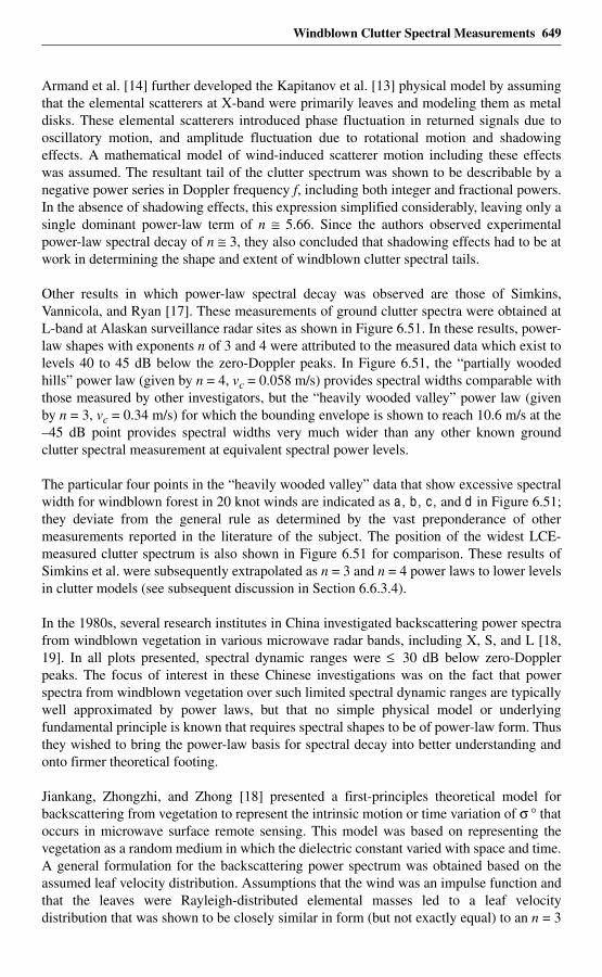
Windblown Clutter Spectral Measurements 649

Armand et al. [14] further developed the Kapitanov et al. [13] physical model by assumingthat the elemental scatterers at X-band were primarily leaves and modeling them as metaldisks. These elemental scatterers introduced phase fluctuation in returned signals due tooscillatory motion, and amplitude fluctuation due to rotational motion and shadowingeffects. A mathematical model of wind-induced scatterer motion including these effectswas assumed. The resultant tail of the clutter spectrum was shown to be describable by anegative power series in Doppler frequency f, including both integer and fractional powers.In the absence of shadowing effects, this expression simplified considerably, leaving only asingle dominant power-law term of n ≅ 5.66. Since the authors observed experimentalpower-law spectral decay of n ≅ 3, they also concluded that shadowing effects had to be atwork in determining the shape and extent of windblown clutter spectral tails.

Other results in which power-law spectral decay was observed are those of Simkins,Vannicola, and Ryan [17]. These measurements of ground clutter spectra were obtained atL-band at Alaskan surveillance radar sites as shown in Figure 6.51. In these results, power-law shapes with exponents n of 3 and 4 were attributed to the measured data which exist tolevels 40 to 45 dB below the zero-Doppler peaks. In Figure 6.51, the “partially woodedhills” power law (given by n = 4, vc = 0.058 m/s) provides spectral widths comparable withthose measured by other investigators, but the “heavily wooded valley” power law (givenby n = 3, vc = 0.34 m/s) for which the bounding envelope is shown to reach 10.6 m/s at the–45 dB point provides spectral widths very much wider than any other known groundclutter spectral measurement at equivalent spectral power levels.

The particular four points in the “heavily wooded valley” data that show excessive spectralwidth for windblown forest in 20 knot winds are indicated as a, b , c , and d in Figure 6.51;they deviate from the general rule as determined by the vast preponderance of othermeasurements reported in the literature of the subject. The position of the widest LCE-measured clutter spectrum is also shown in Figure 6.51 for comparison. These results ofSimkins et al. were subsequently extrapolated as n = 3 and n = 4 power laws to lower levelsin clutter models (see subsequent discussion in Section 6.6.3.4).

In the 1980s, several research institutes in China investigated backscattering power spectrafrom windblown vegetation in various microwave radar bands, including X, S, and L [18,19]. In all plots presented, spectral dynamic ranges were ≤ 30 dB below zero-Dopplerpeaks. The focus of interest in these Chinese investigations was on the fact that powerspectra from windblown vegetation over such limited spectral dynamic ranges are typicallywell approximated by power laws, but that no simple physical model or underlyingfundamental principle is known that requires spectral shapes to be of power-law form. Thusthey wished to bring the power-law basis for spectral decay into better understanding andonto firmer theoretical footing.

Jiankang, Zhongzhi, and Zhong [18] presented a first-principles theoretical model forbackscattering from vegetation to represent the intrinsic motion or time variation of σ ° thatoccurs in microwave surface remote sensing. This model was based on representing thevegetation as a random medium in which the dielectric constant varied with space and time.A general formulation for the backscattering power spectrum was obtained based on theassumed leaf velocity distribution. Assumptions that the wind was an impulse function andthat the leaves were Rayleigh-distributed elemental masses led to a leaf velocitydistribution that was shown to be closely similar in form (but not exactly equal) to an n = 3

650 Windblown Clutter Spectral Measurements

power law. However, the resulting backscattering power spectrum was of “quite complexform” [18]. Its numerical evaluation and comparison with three measured spectra indicatedn = 3 power-law spectral decay over spectral dynamic ranges reaching 30 dB down fromzero-Doppler peaks. A further assumption restricting the originally specified elliptic spatialdistribution of leaf motion to motion only along the wind direction reduced the complexexpression for backscattering power spectrum to the same n = 3 quasi-power-law form asthe leaf velocity distribution. This expression was compared with the Fishbein n = 3 power-law results and found to be in good agreement. The authors concluded by claiming thattheir model provides a theoretical basis for power-law spectral decay and, in addition,allows generalization of parametric effects such as wind speed on spectral shape. Whattheir model appears to show, however, is less far-reaching—only that a postulated n = 3quasi-power-law distribution of leaf velocities results in similar n = 3 quasi-power-lawclutter spectral shapes.

Figure 6.51 Measurements of radar ground clutter power spectra by Simkins, Vannicola, and Ryan of the USAF Rome Air Development Center. After [17], 1977.

–30

–450.02

Doppler Velocity v (m/s)

Rel

ativ

e P

ow

er (

dB

)

n = 4

MountainsPartially Wooded HillsHeavily Wooded Valleys (Lowlands)

n = 4

Measurements Models

L-Band10–20 Knot Winds

0.1 0.2 1 2 3 4 6 8 10

–40

–20

–10

0

10

Power Law, nn = 3

a

b

c

d

a, b, c, d: Extrema : Widest Lincoln Measurement

0.6

Windblown Clutter Spectral Measurements 651

In a later paper, Li [19] summarized L-band investigations at the Chinese Airforce RadarInstitute to characterize Doppler spectra from windblown vegetation to improve design andperformance of MTI and MTD (moving target detector) clutter filters. According to Li, thecommon position reached by Chinese researchers from several research institutes in Chinawas that the radar land clutter spectrum could be represented as a power law with n rangingfrom < 2 to > 3, but that no direct physical explanation for the power-law spectral shapewas available in published papers.

To help provide such an explanation, Li started with the complex theoretical formulationfor the power spectrum from an assemblage of randomly translating and rotating scatterersexpressed as a sum of offset Gaussian functions as derived much earlier by Wong et al.[29], and argued heuristically that the rotational components that spread the spectrumresulted in power-law spectral shapes. To illustrate this hypothesis, Li numericallyevaluated Wong et al.’s expression for three different cases in which Wong et al.’s statisticalparameters were changed to ostensibly show effects of varying wind speed and for twodifferent cases in which the statistical parameters were changed to ostensibly show effectsof changing radar frequency. For all five cases, Li showed that the changing spectral shapesresulting from such parameter variations in Wong et al.’s formula could be well tracked bychanging n in a simple power-law approximation. All such comparisons were shown overspectral dynamic ranges reaching 30 dB below zero-Doppler peaks.

Li finally showed that two of his power-law approximations closely fit, respectively, twospectral measurements taken from the much earlier Rosenbaum and Bowles paper [55].These two measurements were at UHF and L-band and were available to Rosenbaum andBowles (who were Lincoln Laboratory investigators) from a 1972-era Lincoln Laboratoryclutter spectral measurement program [59] to be discussed later. Li selectively showed theRosenbaum and Bowles data only over upper ranges of spectral power (i.e., to –30 dB and–20 dB, respectively, or only over about one-half the spectral dynamic ranges of theoriginal data), and Li also converted the Rosenbaum and Bowles data from a logarithmic toa linear Doppler frequency axis. Li’s resulting plots show results, including bothRosenbaum and Bowles’ experimental data and the power-law approximations to them,which are very linear on 10 log P vs f axes—that is, all would be reasonably matched withexponential functions, although Li matched them with power-law functions.

Measurements of decorrelation times [40], bistatic scattering patterns [41], and powerspectra [42] of continuous-wave X-band backscatter from windblown trees were obtainedby Narayanan and others at the University of Nebraska. These measurements were ofindividual trees (1.8-m-diameter illumination spot size on the tree crown) of variousspecies at very short ranges (e.g., 30 m). Radar system noise is evident in these spectraldata at levels 35 to 45 dB below the zero-Doppler spectral peaks and for Dopplerfrequencies f corresponding to Doppler velocities v ≤ ~1 m/s [42].

Over these relatively limited spectral dynamic ranges and corresponding low Dopplervelocities, many of the measured spectral data appear to closely follow power-law behavior(i.e., the spectral data are very linear as presented on 10 log P vs log f axes), although thisapparent near-power-law behavior was not commented upon in the paper. As with Li [19],the Narayanan et al. starting point in modeling these data was the Wong et al. [29]formulation of the power spectrum for a group of moving scatterers, each with randomrotational as well as translational motion. As previously discussed, Wong et al.’s spectral

652 Windblown Clutter Spectral Measurements

result consists of six Gaussian terms of which four are offset from zero-Doppler. Wonget al.’s expression depends on three parameters, the standard deviation σ d of thetranslational drift velocity components, and the mean and standard deviation σ r of therotational components. Thus in Wong et al.’s expression σ d determines the spectral width ofthe central Gaussian peak at zero-Doppler arising just from translation; determines thelocations of the four offset peaks at ± 2 and ± 4 , respectively; and σ d and σ r togetherdetermine the slower-decaying spectral widths of all five additional Gaussians (four offsetand one not offset from zero-Doppler) arising from rotation.

In modeling his measured power spectral data from windblown trees using Wong et al.’stheoretical expression, Narayanan postulated each of the three parameters σ d, , and σ r tobe linearly dependent on wind speed and specified the coefficients of proportionality foreach specifically by tree type based on least-squared fits to measured autocovariance data.Narayanan et al. also provided extensive conjectural discussion associating σ d with branchtranslational motion and and σ r with leaf/needle rotational motion, although theirresults do not appear to be dependent on the validity of these associations. In this manner,Narayanan et al. arrived at a six-term Gaussian expression for the power spectrum fromwindblown trees based on three coefficients of proportionality to wind speed for which thecoefficients are empirically specified for six different species of trees. This expressionprovided reasonable matches to measured clutter spectral data from individual trees overspectral dynamic ranges reaching 35 to 45 dB below the zero-Doppler peaks.

Narayanan et al. also derived an expression for the MTI improvement factor for a singledelay-line canceller based on their six-term Gaussian expression for the clutter powerspectrum from windblown vegetation, and provided numerical results showing significantdegradation in tree-species-specific delay-line canceller performance using their six-term(i.e., with rotation) spectral expression compared with the corresponding single-Gaussian(i.e., without rotation) spectral expression. In both spectral and improvement factor results,there is considerable variation in these results between different tree species. These short-range small-spot-size deterministic results applicable to specific tree species are in majorcontradistinction to the Phase One and LCE statistical results, which are applicable tolarger cells at longer ranges and over greater spectral dynamic ranges, each cell containinga number of trees, often of mixed species.

A limited set of coherent X-band measurements of ground clutter spectra were obtained byEwell [20] utilizing a different Lincoln Laboratory radar unrelated to the Phase One andLCE radars. This radar (1° beamwidth and 1-µs pulsewidth) was not specifically designedfor measuring very-low-Doppler clutter signals—e.g., it used a cavity-stabilized klystron asthe stable microwave oscillator, which is less stable at low Doppler frequencies thanmodern solid state oscillators. The available ac spectral dynamic range provided by thisradar for measuring clutter signals at low Doppler offsets was ~40 to 45 dB. Measurementswere made of three desert terrain types at ranges for the most part from 3 to 12 km on threedifferent measurement days under winds gusting from 9 to 12 mph. Results were providedfor both circular and linear polarizations.

Over the available ~40-dB spectral dynamic range, these measured data appeared to followpower-law spectral shapes, although with occasional hints in the data of faster decay atlower levels. Table 6.6 shows the resulting power-law shape parameters, averaged over anumber of measurements within each of the three terrain types. These three desert clutter

ωr

ωrωr ωr

ωr

ωr

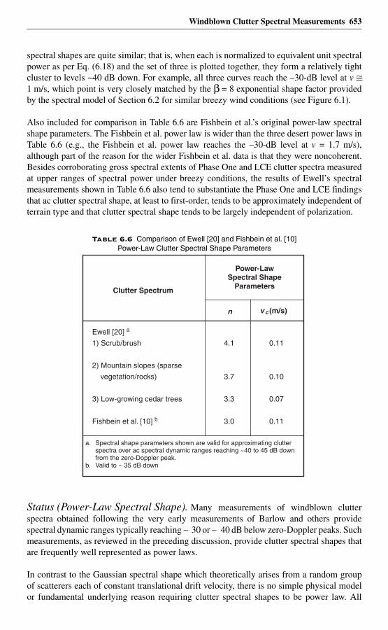
Windblown Clutter Spectral Measurements 653

spectral shapes are quite similar; that is, when each is normalized to equivalent unit spectralpower as per Eq. (6.18) and the set of three is plotted together, they form a relatively tightcluster to levels ~40 dB down. For example, all three curves reach the –30-dB level at v ≅1 m/s, which point is very closely matched by the β = 8 exponential shape factor providedby the spectral model of Section 6.2 for similar breezy wind conditions (see Figure 6.1).

Also included for comparison in Table 6.6 are Fishbein et al.’s original power-law spectralshape parameters. The Fishbein et al. power law is wider than the three desert power laws inTable 6.6 (e.g., the Fishbein et al. power law reaches the –30-dB level at v = 1.7 m/s),although part of the reason for the wider Fishbein et al. data is that they were noncoherent.Besides corroborating gross spectral extents of Phase One and LCE clutter spectra measuredat upper ranges of spectral power under breezy conditions, the results of Ewell’s spectralmeasurements shown in Table 6.6 also tend to substantiate the Phase One and LCE findingsthat ac clutter spectral shape, at least to first-order, tends to be approximately independent ofterrain type and that clutter spectral shape tends to be largely independent of polarization.

Status (Power-Law Spectral Shape). Many measurements of windblown clutterspectra obtained following the very early measurements of Barlow and others providespectral dynamic ranges typically reaching ∼ 30 or ∼ 40 dB below zero-Doppler peaks. Suchmeasurements, as reviewed in the preceding discussion, provide clutter spectral shapes thatare frequently well represented as power laws.

In contrast to the Gaussian spectral shape which theoretically arises from a random groupof scatterers each of constant translational drift velocity, there is no simple physical modelor fundamental underlying reason requiring clutter spectral shapes to be power law. All

Table 6.6 Comparison of Ewell [20] and Fishbein et al. [10] Power-Law Clutter Spectral Shape Parameters

Clutter Spectrum

Power-LawSpectral Shape

Parameters

n v c (m/s)

Ewell [20] a

1) Scrub/brush

2) Mountain slopes (sparse

vegetation/rocks)

3) Low-growing cedar trees

Fishbein et al. [10] b

4.1

3.7

3.3

3.0

0.11

0.10

0.07

0.11

a. Spectral shape parameters shown are valid for approximating clutter spectra over ac spectral dynamic ranges reaching ~40 to 45 dB down from the zero-Doppler peak.b. Valid to ~ 35 dB down

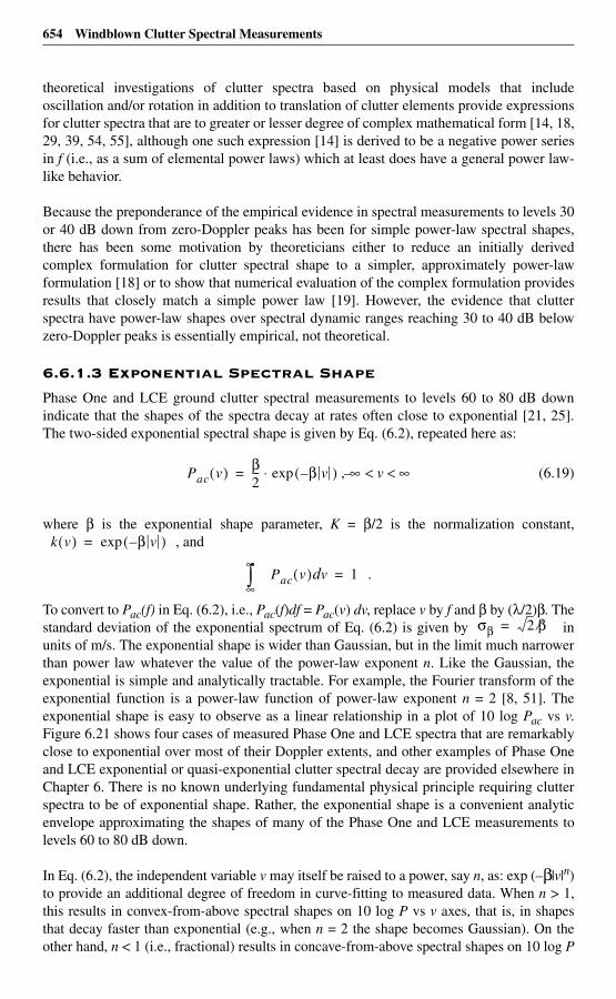
654 Windblown Clutter Spectral Measurements

theoretical investigations of clutter spectra based on physical models that includeoscillation and/or rotation in addition to translation of clutter elements provide expressionsfor clutter spectra that are to greater or lesser degree of complex mathematical form [14, 18,29, 39, 54, 55], although one such expression [14] is derived to be a negative power seriesin f (i.e., as a sum of elemental power laws) which at least does have a general power law-like behavior.

Because the preponderance of the empirical evidence in spectral measurements to levels 30or 40 dB down from zero-Doppler peaks has been for simple power-law spectral shapes,there has been some motivation by theoreticians either to reduce an initially derivedcomplex formulation for clutter spectral shape to a simpler, approximately power-lawformulation [18] or to show that numerical evaluation of the complex formulation providesresults that closely match a simple power law [19]. However, the evidence that clutterspectra have power-law shapes over spectral dynamic ranges reaching 30 to 40 dB belowzero-Doppler peaks is essentially empirical, not theoretical.

6.6.1.3 Exponential Spectral Shape

Phase One and LCE ground clutter spectral measurements to levels 60 to 80 dB downindicate that the shapes of the spectra decay at rates often close to exponential [21, 25].The two-sided exponential spectral shape is given by Eq. (6.2), repeated here as:

, (6.19)

where β is the exponential shape parameter, K = β/2 is the normalization constant,, and

.

To convert to Pac(f) in Eq. (6.2), i.e., Pac(f)df = Pac(v) dv, replace v by f and β by (λ/2)β. Thestandard deviation of the exponential spectrum of Eq. (6.2) is given by inunits of m/s. The exponential shape is wider than Gaussian, but in the limit much narrowerthan power law whatever the value of the power-law exponent n. Like the Gaussian, theexponential is simple and analytically tractable. For example, the Fourier transform of theexponential function is a power-law function of power-law exponent n = 2 [8, 51]. Theexponential shape is easy to observe as a linear relationship in a plot of 10 log Pac vs v.Figure 6.21 shows four cases of measured Phase One and LCE spectra that are remarkablyclose to exponential over most of their Doppler extents, and other examples of Phase Oneand LCE exponential or quasi-exponential clutter spectral decay are provided elsewhere inChapter 6. There is no known underlying fundamental physical principle requiring clutterspectra to be of exponential shape. Rather, the exponential shape is a convenient analyticenvelope approximating the shapes of many of the Phase One and LCE measurements tolevels 60 to 80 dB down.

In Eq. (6.2), the independent variable v may itself be raised to a power, say n, as: exp (–β|v|n)to provide an additional degree of freedom in curve-fitting to measured data. When n > 1,this results in convex-from-above spectral shapes on 10 log P vs v axes, that is, in shapesthat decay faster than exponential (e.g., when n = 2 the shape becomes Gaussian). On theother hand, n < 1 (i.e., fractional) results in concave-from-above spectral shapes on 10 log P

Pac v( ) β2--- β v–( )exp⋅= ∞ v ∞< <–

k v( ) β v–( )exp=

Pac v( ) vd∞–

∞∫ 1=

σβ 2 β⁄=

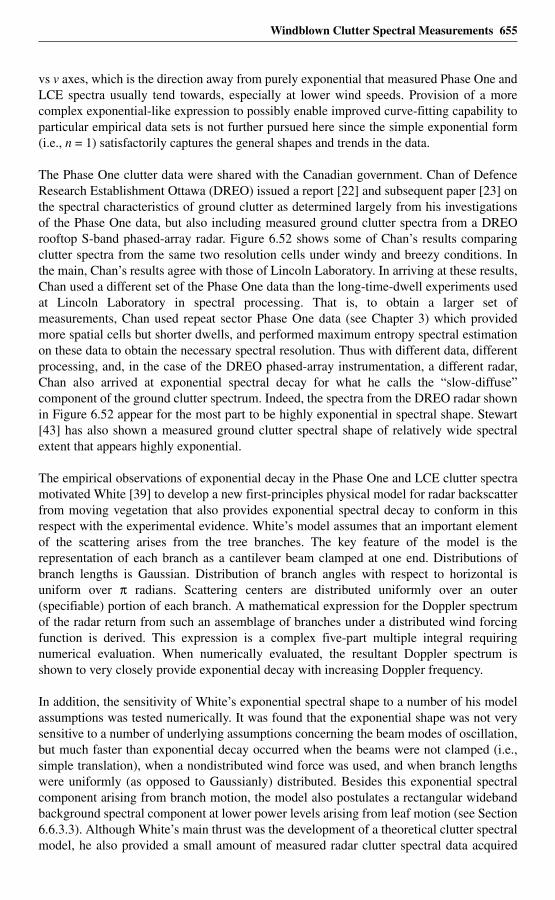
Windblown Clutter Spectral Measurements 655

vs v axes, which is the direction away from purely exponential that measured Phase One andLCE spectra usually tend towards, especially at lower wind speeds. Provision of a morecomplex exponential-like expression to possibly enable improved curve-fitting capability toparticular empirical data sets is not further pursued here since the simple exponential form(i.e., n = 1) satisfactorily captures the general shapes and trends in the data.

The Phase One clutter data were shared with the Canadian government. Chan of DefenceResearch Establishment Ottawa (DREO) issued a report [22] and subsequent paper [23] onthe spectral characteristics of ground clutter as determined largely from his investigationsof the Phase One data, but also including measured ground clutter spectra from a DREOrooftop S-band phased-array radar. Figure 6.52 shows some of Chan’s results comparingclutter spectra from the same two resolution cells under windy and breezy conditions. Inthe main, Chan’s results agree with those of Lincoln Laboratory. In arriving at these results,Chan used a different set of the Phase One data than the long-time-dwell experiments usedat Lincoln Laboratory in spectral processing. That is, to obtain a larger set ofmeasurements, Chan used repeat sector Phase One data (see Chapter 3) which providedmore spatial cells but shorter dwells, and performed maximum entropy spectral estimationon these data to obtain the necessary spectral resolution. Thus with different data, differentprocessing, and, in the case of the DREO phased-array instrumentation, a different radar,Chan also arrived at exponential spectral decay for what he calls the “slow-diffuse”component of the ground clutter spectrum. Indeed, the spectra from the DREO radar shownin Figure 6.52 appear for the most part to be highly exponential in spectral shape. Stewart[43] has also shown a measured ground clutter spectral shape of relatively wide spectralextent that appears highly exponential.

The empirical observations of exponential decay in the Phase One and LCE clutter spectramotivated White [39] to develop a new first-principles physical model for radar backscatterfrom moving vegetation that also provides exponential spectral decay to conform in thisrespect with the experimental evidence. White’s model assumes that an important elementof the scattering arises from the tree branches. The key feature of the model is therepresentation of each branch as a cantilever beam clamped at one end. Distributions ofbranch lengths is Gaussian. Distribution of branch angles with respect to horizontal isuniform over π radians. Scattering centers are distributed uniformly over an outer(specifiable) portion of each branch. A mathematical expression for the Doppler spectrumof the radar return from such an assemblage of branches under a distributed wind forcingfunction is derived. This expression is a complex five-part multiple integral requiringnumerical evaluation. When numerically evaluated, the resultant Doppler spectrum isshown to very closely provide exponential decay with increasing Doppler frequency.

In addition, the sensitivity of White’s exponential spectral shape to a number of his modelassumptions was tested numerically. It was found that the exponential shape was not verysensitive to a number of underlying assumptions concerning the beam modes of oscillation,but much faster than exponential decay occurred when the beams were not clamped (i.e.,simple translation), when a nondistributed wind force was used, and when branch lengthswere uniformly (as opposed to Gaussianly) distributed. Besides this exponential spectralcomponent arising from branch motion, the model also postulates a rectangular widebandbackground spectral component at lower power levels arising from leaf motion (see Section6.6.3.3). Although White’s main thrust was the development of a theoretical clutter spectralmodel, he also provided a small amount of measured radar clutter spectral data acquired

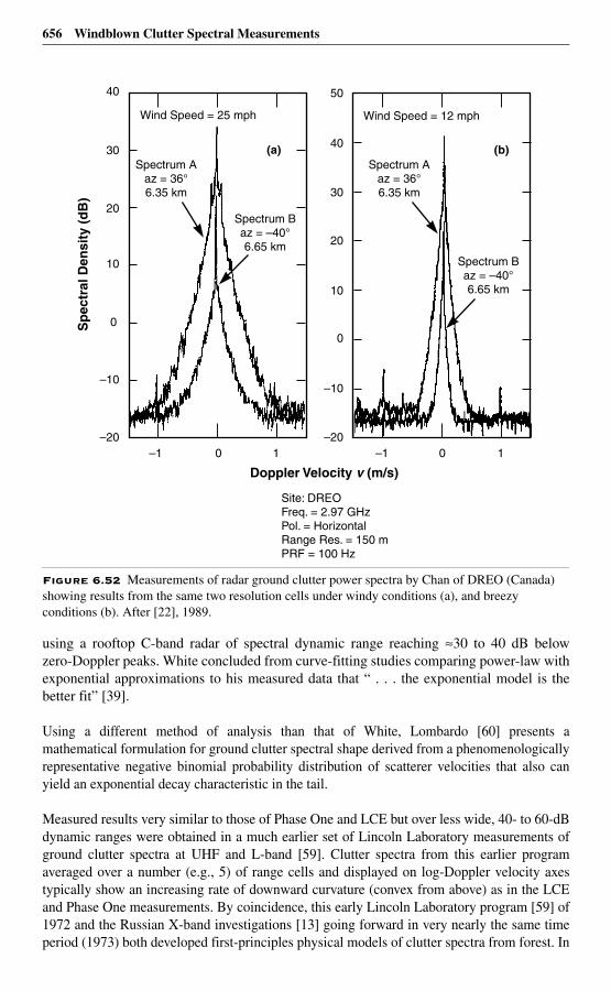
656 Windblown Clutter Spectral Measurements

using a rooftop C-band radar of spectral dynamic range reaching ≈30 to 40 dB belowzero-Doppler peaks. White concluded from curve-fitting studies comparing power-law withexponential approximations to his measured data that “ . . . the exponential model is thebetter fit” [39].

Using a different method of analysis than that of White, Lombardo [60] presents amathematical formulation for ground clutter spectral shape derived from a phenomenologicallyrepresentative negative binomial probability distribution of scatterer velocities that also canyield an exponential decay characteristic in the tail.

Measured results very similar to those of Phase One and LCE but over less wide, 40- to 60-dBdynamic ranges were obtained in a much earlier set of Lincoln Laboratory measurements ofground clutter spectra at UHF and L-band [59]. Clutter spectra from this earlier programaveraged over a number (e.g., 5) of range cells and displayed on log-Doppler velocity axestypically show an increasing rate of downward curvature (convex from above) as in the LCEand Phase One measurements. By coincidence, this early Lincoln Laboratory program [59] of1972 and the Russian X-band investigations [13] going forward in very nearly the same timeperiod (1973) both developed first-principles physical models of clutter spectra from forest. In

Figure 6.52 Measurements of radar ground clutter power spectra by Chan of DREO (Canada) showing results from the same two resolution cells under windy conditions (a), and breezy conditions (b). After [22], 1989.

–1 0–20

–10

0

30

40

Doppler Velocity v (m/s)

Sp

ectr

al D

ensi

ty (

dB

)

10

1

Spectrum Baz = –40°6.65 km

Spectrum Baz = –40°6.65 km

Spectrum Aaz = 36°6.35 km

Spectrum Aaz = 36°6.35 km

Site: DREOFreq. = 2.97 GHzPol. = HorizontalRange Res. = 150 mPRF = 100 Hz

20

Wind Speed = 25 mph

–1 0 1

Wind Speed = 12 mph

–20

–10

0

30

40

10

20

50

(a) (b)

Windblown Clutter Spectral Measurements 657

both studies, the tree was modeled as a mechanical resonator excited by a turbulent wind fieldof known spectral content. Both programs involved measurements of tree motion. In bothprograms, the spectral content of tree motion decayed at low frequencies below a resonancemaximum according to an n = 5/3 power law; at higher frequencies above the resonancemaximum, the decay was faster. The slightly later (1974), largely theoretical paper by LincolnLaboratory authors [55] concerning electromagnetic scattering from vegetative regionsincluded three measured clutter spectra from the 1972-era measurement program.

Shoulders before the onset of faster decay, such as those shown in some of the LCE- andPhase One-measured clutter spectra (e.g., see Figures 6.22, 6.24, and 6.25), are similar tothose observed previously in the earlier Lincoln Laboratory program [59] and explained aslocal resonance maxima associated with the natural resonant frequency of trees. Theresonance shoulder was more pronounced at lower frequencies and lower wind speeds, andtended to diminish at higher frequencies and higher wind speeds. The reason is that, atlower wind speeds and longer wavelengths, the motion of the tree is a small fraction of aradar wavelength. Thus under these conditions the tree motion superimposes a phasemodulation with low index of modulation, and as a result the clutter spectrum directlycorresponds with that of the tree’s physical motion. At higher frequencies and understronger winds, the degree of phase modulation increases and the clutter spectrum nolonger simply replicates that of the tree motion. These observations tend to be corroboratedin LCE and Phase One results. In addition, the LCE and Phase One data tend to haveresonance shoulders to somewhat higher frequencies in measurements from partially openor open terrain (desert, farmland, rangeland) in which there is a significant dc component;the measurements from forested terrain tend to have distinct resonance shoulders only atthe lower radar frequencies (VHF and UHF). The earlier Lincoln Laboratory programobserved, in passing, that the shapes of some measured spectra beyond the resonanceshoulder were highly exponential, but this observation was not elaborated upon.

Another early, more explicit, observation of exponential spectral shape is in the results ofAndrianov, Armand, and Kibardina [16] (see Figure 6.50). In these results, exponentialdecay was initially observed from the maximum zero-Doppler level down to –20 dB,followed by power-law decay thereafter to –70 dB with reported values of n equal to 3.4,3.8, and 5.6 for pine, alder, and birch, respectively. The equipment used was ostensibly of70-dB dynamic range [15] although, to use their words translated to English, two dynamicrange intervals were “sewn together” [16], as shown in Figure 6.49, to provide the full 70-dBrange. In terms of gross spectral extent (e.g., 1.5 m/s, 70 dB down; 0.4 m/s, 20 dB down),these results of Andrianov et al. [15, 16] fall closely within the range of measured LCE andPhase One spectral extents over similar spectral dynamic ranges. The earlier results ofKapitanov, Mel’nichuk, and Chernikov [13], as shown in Figure 6.48, were said to exhibitGaussian decay down 10 to 15 dB, followed by power-law decay with n = 4 down to –40 dB.The initial Gaussian decay was later stated to be erroneous by Andrianov et al. [16] becauseof early equipment limitations and that initial exponential decay as reported by them (seeFigure 6.50) was more correct.

The exponent n of the power law is easy to estimate in measured spectral data as simply one-tenth the slope of the approximating straight line on 10 log P vs log v axes in dB/decade. InFigure 6.50, the three measured spectral curves for pine, alder, and birch shown to the left donot exhibit decay anything like the quoted power-law slopes of n = 3.4, 3.8, and 5.6,respectively. These three curves are stated by the authors to be three particular examples of

658 Windblown Clutter Spectral Measurements

measured spectra, whereas their quoted values of n are averages over all measurements inwhich the value of n varies from 2.6 to 6.8. The rates of decay in the spectral tails of the datato the left in Figure 6.50 are much greater than any of these quoted values of n and, at leastin qualitative appearance (increasing downward curvature), appear to be more exponentialthan power law. The data of Figure 6.49 appear to be more credibly of power-law behavior(n ≈6) in their tails, but the data plotted at the –68-dB level indicate slightly increasingcurvature (rate of decay > n ≈6) at the lowest power levels shown. The data of Figure 6.48closely match the n = 4 power law attributed by the authors to these data.

Some confusion may arise because these Russian investigators [13–16] associate power-law shapes with lower ranges of spectral power in their measured data, whereas otherinvestigators [10–12, 17–20] match their data to power-law shapes over upper ranges ofspectral power. Measured clutter data in any particular regime of spectral power may befitted with a power law, but the danger lies in extrapolating the power law beyond its regimeof applicability.

An additional, somewhat more significant, past use of the exponential function tocharacterize clutter spectra from windblown vegetation occurred in experimental workperformed at the Laboratoire Central de Telecommunications in France [38]. These Frenchmeasurements were also performed during the 1970s using coherent-on-receive radars,spectrum analyzers with limited (i.e., 50 dB) dynamic range, and a limited number ofvegetation clutter types. In this work, the MTI filter cutoff frequency was adjusted so as tobe just sufficient to remove the clutter to the –40-dB level. It was found that the cutofffrequency just sufficient to remove the clutter was best predicted by hypothesizing anexponential spectral clutter model. The cutoff frequency predicted by a Gaussian spectralmodel was too low (i.e., optimistic—if there was even a light wind, significant clutter waspassed by the filter); whereas the cutoff frequency predicted by a power-law spectral modelwas too high (i.e., pessimistic—at X-band, all targets with radial speed < 50 km/h weremissed). In contrast, cutoff frequencies in the range predicted by an exponential spectralmodel were successfully used as the standard specification for many service radars in theFrench military and elsewhere.

Status (Exponential Spectral Shape). The significantly increasing rate ofdownward curvature (i.e., convex from above) observed in the general shapes of PhaseOne- and LCE-measured windblown ground clutter Doppler spectra on 10 log P vs log vaxes over spectral dynamic ranges reaching 60 to 80 dB below zero-Doppler peaks pointsto a general exponential characterization rather than a power-law characterization that plotslinearly on such axes. Increasing rate of downward curvature in such plots has always beenobserved without exception in all measurements examined of clutter spectra fromwindblown trees and other vegetation under breezy or windy conditions taken from theseextensive databases. Other investigators [22, 24] have corroborated that the exponentialshape factor is generally representative of these data and is not the result of processing-specific particulars.

In early studies, theoretical investigators attempted to reduce complex mathematicalformulations of clutter spectra based on physical models incorporating oscillation and/orshadowing of elemental scatterers to simple power-law forms to conform with theexperimental evidence then available at upper levels of spectral power (down 30 or 40 dBfrom zero-Doppler peaks). Subsequent awareness of investigators of the LincolnLaboratory clutter spectral results provided motivation to develop theoretical bases for the

Windblown Clutter Spectral Measurements 659

observed exponential spectral shapes. Thus there exist the interesting works of White [39]and Lombardo [60] in which formulations are developed for the clutter Doppler spectrum,that, although mathematically complex, provide close to exponential decay undernumerical evaluation. In addition, White observed that “the series solutions produced byBass et al. [54], Armand et al. [14], and Wong et al. [29] probably have sufficient degrees offreedom to produce a function that would be a close approximation to . . . exponential . . . ”[39]. Nevertheless, as for the power law for spectral dynamic ranges 30 to 40 dB down, theevidence of exponential clutter spectral shape for spectral dynamic ranges reaching 60 to80 dB down is essentially empirical.

The only known measurements of windblown clutter spectra of spectral dynamic rangesequal to or exceeding those of the Phase One and LCE instruments are the Russianmeasurements of the 1970s [13–16], for which the results over lower ranges of spectralpower were approximated as power laws. However, these results are power law only in apiece-part sense; the upper range of spectral power was concluded to be exponential. Hencethese results are not very useful or analytically tractable, in that no single simple analyticfunction was provided to describe the complete clutter spectral shape over its full measuredspectral dynamic range. Furthermore, little actual measurement data were shown in thesepapers, thus restricting possibilities for independent assessment of the data and conclusionsby present-day readers.

Like the Gaussian function, the exponential function is simple and analytically tractable.The exponential function provides spectral shapes that are wider than Gaussian, as requiredby all the empirical evidence and by theoretical constructs involving oscillation, rotation,and shadowing of clutter elements; that are very much narrower at lower power levels (60to 80 dB down) than extrapolations to lower levels of power-law representations ofmeasurements accurate at higher levels of spectral power (30 to 40 dB down); and that arereasonably equivalent to the measurement data at high and low levels of spectral power.

6.6.2 Reconciliation of Exponential Shape with Historical Results

6.6.2.1 Current vs Historical Clutter Spectral Measurements

Figure 6.5 (Section 6.3.2.1) shows a measured LCE clutter spectrum from windblowntrees and compares it with several exponential shape functions (dotted lines) of variousvalues of exponential shape parameter β. In Figure 6.5, the measured data closely followthe exponential curve of shape parameter β = 5.2 over the full spectral dynamic rangeshown. Also shown in Figure 6.5 is a narrower Gaussian spectral shape function (dashedline) corresponding to Barlow’s much-referenced historical measurement [7] (see Figure6.45). The Gaussian curve in the figure is shown extrapolated to low spectral power levelsmuch below Barlow’s measured spectral dynamic range, which reached only 20 dB belowthe zero-Doppler peak. The overall rate of decay in the LCE data of Figure 6.5 is muchmore exponential than Gaussian in character. Spectral tails wider than Gaussian aretheoretically required by branches and leaves in oscillatory motion [19, 29] (seeSection 6.6.1).

Figure 6.53 shows another LCE windblown-tree clutter spectrum different from that ofFigure 6.5. The spectrum of Figure 6.53 was measured at vertical polarization on 11

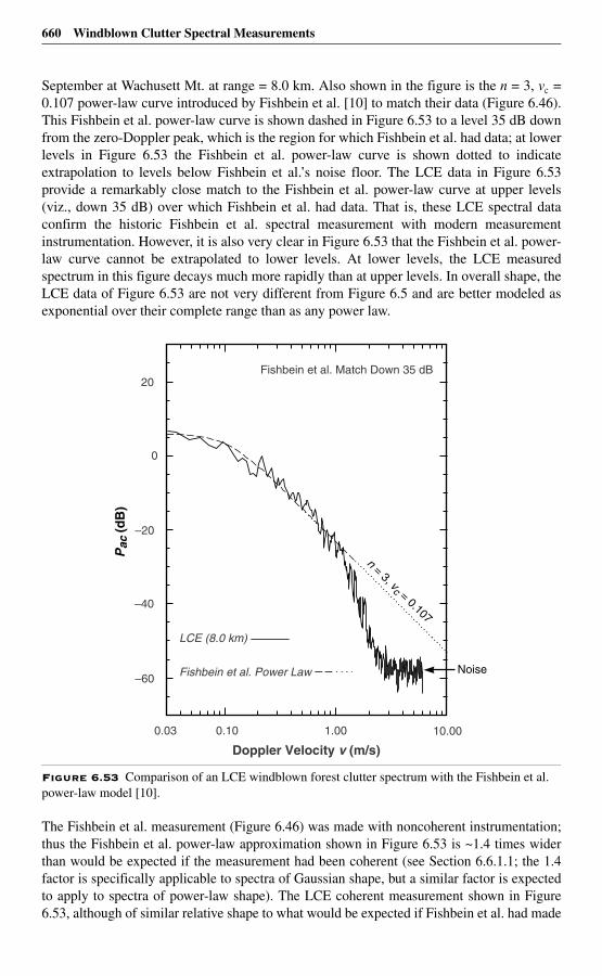
660 Windblown Clutter Spectral Measurements

September at Wachusett Mt. at range = 8.0 km. Also shown in the figure is the n = 3, vc =0.107 power-law curve introduced by Fishbein et al. [10] to match their data (Figure 6.46).This Fishbein et al. power-law curve is shown dashed in Figure 6.53 to a level 35 dB downfrom the zero-Doppler peak, which is the region for which Fishbein et al. had data; at lowerlevels in Figure 6.53 the Fishbein et al. power-law curve is shown dotted to indicateextrapolation to levels below Fishbein et al.’s noise floor. The LCE data in Figure 6.53provide a remarkably close match to the Fishbein et al. power-law curve at upper levels(viz., down 35 dB) over which Fishbein et al. had data. That is, these LCE spectral dataconfirm the historic Fishbein et al. spectral measurement with modern measurementinstrumentation. However, it is also very clear in Figure 6.53 that the Fishbein et al. power-law curve cannot be extrapolated to lower levels. At lower levels, the LCE measuredspectrum in this figure decays much more rapidly than at upper levels. In overall shape, theLCE data of Figure 6.53 are not very different from Figure 6.5 and are better modeled asexponential over their complete range than as any power law.

The Fishbein et al. measurement (Figure 6.46) was made with noncoherent instrumentation;thus the Fishbein et al. power-law approximation shown in Figure 6.53 is ~1.4 times widerthan would be expected if the measurement had been coherent (see Section 6.6.1.1; the 1.4factor is specifically applicable to spectra of Gaussian shape, but a similar factor is expectedto apply to spectra of power-law shape). The LCE coherent measurement shown in Figure6.53, although of similar relative shape to what would be expected if Fishbein et al. had made

Figure 6.53 Comparison of an LCE windblown forest clutter spectrum with the Fishbein et al. power-law model [10].

0.03 1.00 10.00

–60

–40

–20

0

20

Doppler Velocity v (m/s)

Pac

(dB

)

LCE (8.0 km)

0.10

NoiseFishbein et al. Power Law

n = 3, vc = 0.107

Fishbein et al. Match Down 35 dB

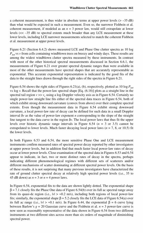
Windblown Clutter Spectral Measurements 661

a coherent measurement, is thus wider in absolute terms at upper power levels (> –35 dB)than what would be expected in such a measurement. Even so, the narrower Fishbein et al.coherent measurement, if modeled as an n = 3 power law, would still extrapolate at lowerlevels (<< –35 dB) to spectral extents much broader than any LCE measurement at theselower levels, including LCE narrower measurements selected to match the coherent Fishbeinet al. measurement at upper power levels.

Figure 6.21 (Section 6.4.2) shows measured LCE and Phase One clutter spectra as 10 logPtot vs v from cells containing windblown trees on breezy and windy days. These results areamong the widest windblown clutter spectra measured by these instruments. In contrastwith most of the other historical spectral measurements discussed in Section 6.6.1, themeasurements of Figure 6.21 over greater spectral dynamic ranges than were available inmost of the other measurements have spectral shapes that are accurately representable asexponential. This accurate exponential representation is indicated by the good fits of thedata to the straight lines drawn through the right sides of the spectra in Figure 6.21.

Figure 6.54 shows the right sides of Figures 6.21(a), (b), respectively, plotted as 10 log Ptotvs log v. Recall that the power-law spectral shape [Eq. (6.18)] plots as a straight line in thespectral tail region v >> vc using a log-Doppler velocity axis as in Figure 6.54. Certainly nosingle power-law straight line fits either of the spectral data traces in Figure 6.54, both ofwhich exhibit strong downward curvature (convex from above) over their complete spectralextents. Even though the measurement data in Figure 6.54 exhibit strong downwardcurvature, a local power-law rate of decay can be defined for such data in a small Dopplerinterval δv as the value of power-law exponent n corresponding to the slope of the straightline tangent to the data curve in the region δv. The local power laws that thus fit the upperlevels over historic dynamic range intervals in Figure 6.54 (n = 3 or 3.5) cannot beextrapolated to lower levels. Much faster decaying local power laws (n = 7, 8, or 10.5) fitthe lower levels.

In both Figures 6.53 and 6.54, the more sensitive Phase One and LCE measurementinstruments confirm measured rates of spectral power decay reported by other investigatorsat upper power levels, but in addition find that much faster local power-law rates of decayoccur at lower power levels. Close examination of the spectral data in Figures 6.53 and 6.54appear to indicate, in fact, two or more distinct rates of decay in the spectra, perhapsindicating different phenomenological regimes with different sets of scatterers and/ordifferent mechanisms of scatter dominating at different spectral power levels. On the basisof these results, it is not surprising that many previous investigators have characterized therate of ground clutter spectral decay at relatively high spectral power levels (i.e., 35 to45 dB down) as n = 3 or n = 4 power laws.

In Figure 6.54, exponential fits to the data are shown lightly dotted. The exponential shapeβ = 7.1 closely fits the Phase One data of Figure 6.54(b) over its full ac spectral range awayfrom its quasi-dc region (i.e., |v| > ≈0.2 m/s), including both regions of local power-lawfits; similarly, the exponential shape β = 5.2 closely fits the LCE data of Figure 6.54(a) overits full ac range (i.e., |v| > ≈0.1 m/s). In Figure 6.44, the exponential β = 6 curve lyingbetween Barlow’s g = 20 Gaussian curve and the Fishbein et al. n = 3 power-law curve isnow seen as reasonably representative of the data shown in Figure 6.54 from two differentinstruments at two different sites across more than six orders of magnitude of diminishingspectral power.

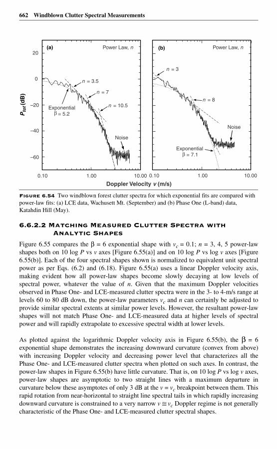
662 Windblown Clutter Spectral Measurements

6.6.2.2 Matching Measured Clutter Spectra with Analytic Shapes

Figure 6.55 compares the β = 6 exponential shape with vc = 0.1; n = 3, 4, 5 power-lawshapes both on 10 log P vs v axes [Figure 6.55(a)] and on 10 log P vs log v axes [Figure6.55(b)]. Each of the four spectral shapes shown is normalized to equivalent unit spectralpower as per Eqs. (6.2) and (6.18). Figure 6.55(a) uses a linear Doppler velocity axis,making evident how all power-law shapes become slowly decaying at low levels ofspectral power, whatever the value of n. Given that the maximum Doppler velocitiesobserved in Phase One- and LCE-measured clutter spectra were in the 3- to 4-m/s range atlevels 60 to 80 dB down, the power-law parameters vc and n can certainly be adjusted toprovide similar spectral extents at similar power levels. However, the resultant power-lawshapes will not match Phase One- and LCE-measured data at higher levels of spectralpower and will rapidly extrapolate to excessive spectral width at lower levels.

As plotted against the logarithmic Doppler velocity axis in Figure 6.55(b), the β = 6exponential shape demonstrates the increasing downward curvature (convex from above)with increasing Doppler velocity and decreasing power level that characterizes all thePhase One- and LCE-measured clutter spectra when plotted on such axes. In contrast, thepower-law shapes in Figure 6.55(b) have little curvature. That is, on 10 log P vs log v axes,power-law shapes are asymptotic to two straight lines with a maximum departure incurvature below these asymptotes of only 3 dB at the v = vc breakpoint between them. Thisrapid rotation from near-horizontal to straight line spectral tails in which rapidly increasingdownward curvature is constrained to a very narrow v ≅ vc Doppler regime is not generallycharacteristic of the Phase One- and LCE-measured clutter spectral shapes.

Figure 6.54 Two windblown forest clutter spectra for which exponential fits are compared with power-law fits: (a) LCE data, Wachusett Mt. (September) and (b) Phase One (L-band) data, Katahdin Hill (May).

1.00 10.00

–60

–40

–20

0

20

Exponential = 5.2

Exponential = 7.1

0.10

n = 3.5

n = 7

n = 10.5

Power Law, n Power Law, n

Noise

Doppler Velocity v (m/s)

Pto

t (d

B)

1.00 10.000.10

n = 3

n = 8

Noise

(a) (b)

Windblown Clutter Spectral Measurements 663

6.6.2.3 Summary

The Phase One and LCE measurements of ground clutter spectra presented in Chapter 6are displayed on both linear and logarithmic Doppler velocity axes. What is clear in thesepresentations, and what has not been generally recognized, is that if the clutter ac spectralshape Pac is represented as a power law, the power-law exponent n is not constant butgradually increases from n = 3 or 4 when Pac is 35 or 40 dB down from its maximum ton = 5 or 6 or even higher when Pac is 60 to 80 dB down from its maximum. Uncertaintyabout whether “the law” of spectral decay is “n = 3 or n = 6 (or even exponential)” isabetted by the additional lack of general recognition that the shape of the spectrum tolevels 60 to 80 dB down is usually not precisely representable by any single analyticexpression. In the results presented herein, slight upward curvature (concave from above)often occurs on the 10 log Pac vs v plots, hence the shape can be slightly broader thanexponential; whereas strong downward curvature (convex from above) almost alwaysoccurs on the 10 log Pac vs log v plots, hence the shape is much narrower than constantpower law.

Thus there is no argument with Andrianov, Armand, and Kibardina that “It is [usually]impossible to [precisely match] the spectral density of the scattered signal by a singleanalytical function in the entire range of [Doppler] frequencies” [16]. However, much ofthe potentially ensuing difficulty in the general modeling of clutter spectra is overcome inChapter 6 not just by utilizing exponential shapes, but also by introducing the concept of aquasi-dc region and absorbing excess power in this region into the dc delta function termof the model (see also [31]). However the spectrum is modeled, the Phase One and LCEresults support the general existence of windblown clutter Doppler velocities only as greatas ∼ 3 to 4 m/s for 15- to 30-mph winds to levels 70 to 80 dB down.

Figure 6.55 Comparison of exponential and power-law spectral shapes: (a) linear and (b) logarithmic Doppler velocity axes.

0.10 1.00 10.00

–80

–60

–40

–20

0

0 5 10

Pac

(d

B)

n = 3

n = 4

n = 5 = 6 Exponential = 6

n = 3

n = 4n = 5

vc = 0.1 m/s vc = 0.1 m/s

Doppler Velocity v (m/s)

(a) (b)

Power Law, n Power Law, n

664 Windblown Clutter Spectral Measurements

The evidence for both power-law and exponential clutter spectral shapes is essentiallyempirical. The concern in Chapter 6 is not which of these two forms fits the data best overspectral dynamic ranges of –30 or –40 dB, or even whether such a question can bedefinitively answered. Chapter 6 provides good examples of both power-law andexponential fits to measured clutter spectral data to levels 30 or 40 dB down, and inreviewing the technical literature finds it to be similarly bipartite on this matter. Theconcern is, however, in determining an appropriate functional form to describe clutterspectra over greater spectral dynamic ranges. The main observation in this regard, based onthe Phase One and LCE databases, is that no matter how good the power-law fits are overspectral dynamic ranges extending 30 to 40 dB below zero-Doppler peaks, they cannot beextrapolated to lower levels. That is, power-law shapes extrapolate rapidly to excessivespectral width. In contrast, the exponential form generally represents the Phase One andLCE measurements not only over their upper ranges of spectral power but also over theircomplete spectral dynamic ranges extending to levels 60 to 80 dB below zero-Dopplerpeaks. Thus radar system design for which ground clutter interference is of consequence atsuch low levels of spectral power is much more accurately based on an exponential clutterspectral shape approximation than on an extrapolated power-law approximation. Thevalidity of the exponential shape on the basis of best matching coherent detection systemperformance to that obtained using actual measured I/Q clutter data as input to the clutterprocessor is demonstrated in Section 6.5.4.

6.6.3 Reports of Unusually Long Spectral TailsSeveral historical reports of spectral tails in ground clutter at unusually high power levels and/or extending to unusually high Doppler velocities are considered in the following subsections.

6.6.3.1 Total Environment Clutter

There exists significant concern with how to characterize the clutter residues left inDoppler filter banks in high sensitivity radars after MTI cancellation that might cause falsetargets for subsequent multitarget tracking algorithms. Thus there is interest in specifyingan overall environment clutter model that would include the Doppler interference fromsuch things as aurora, meteor trails, cosmic noise, windblown material (leaves, dust, spray),birds and insects, rotating structures, rain and other precipitation, lightning, clear airturbulence, fluctuations of refractive index, etc. Often such phenomena are highly transientas they occur in measurements of radar Doppler spectra, so that it is difficult to causally andquantitatively associate unusual spectral artifacts directly with their sources. It is notsuggested here that a specific program dedicated to measuring any one of these phenomenawould not be successful—rather, that in a general database of spectral measurementscollected from spatial ensembles of remote ground clutter cells, the occasional occurrenceof causative agents different from windblown vegetation is difficult to determine. The mainfocus of interest in the Phase One and LCE spectral measurements is the general andcontinuous spectral spreading that occurs in ground clutter due to wind-induced motion oftree foliage and branches or other vegetative land cover. These clutter databases have notbeen very extensively used for systematic searching for infrequent, spatially unusual,narrowband, or transient spectral features resulting from other causative agents in the totalclutter environment because of their ephemeral nature and uncertain signaturecharacteristics, although occasional evidence of birds, airplanes, automobiles, and otheranomalies has been encountered in the spectral analyses of these data. The one concreteexample encountered by the LCE radar of clutter from the total environment over land with

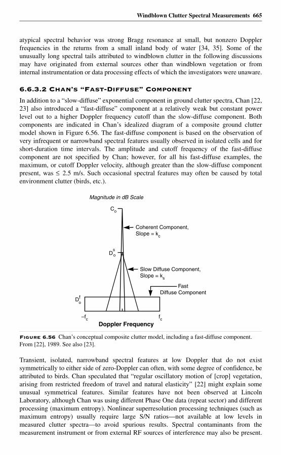
Windblown Clutter Spectral Measurements 665

atypical spectral behavior was strong Bragg resonance at small, but nonzero Dopplerfrequencies in the returns from a small inland body of water [34, 35]. Some of theunusually long spectral tails attributed to windblown clutter in the following discussionsmay have originated from external sources other than windblown vegetation or frominternal instrumentation or data processing effects of which the investigators were unaware.

6.6.3.2 Chan’s “Fast-Diffuse” Component

In addition to a “slow-diffuse” exponential component in ground clutter spectra, Chan [22,23] also introduced a “fast-diffuse” component at a relatively weak but constant powerlevel out to a higher Doppler frequency cutoff than the slow-diffuse component. Bothcomponents are indicated in Chan’s idealized diagram of a composite ground cluttermodel shown in Figure 6.56. The fast-diffuse component is based on the observation ofvery infrequent or narrowband spectral features usually observed in isolated cells and forshort-duration time intervals. The amplitude and cutoff frequency of the fast-diffusecomponent are not specified by Chan; however, for all his fast-diffuse examples, themaximum, or cutoff Doppler velocity, although greater than the slow-diffuse componentpresent, was ≤ 2.5 m/s. Such occasional spectral features may often be caused by totalenvironment clutter (birds, etc.).

Transient, isolated, narrowband spectral features at low Doppler that do not existsymmetrically to either side of zero-Doppler can often, with some degree of confidence, beattributed to birds. Chan speculated that “regular oscillatory motion of [crop] vegetation,arising from restricted freedom of travel and natural elasticity” [22] might explain someunusual symmetrical features. Similar features have not been observed at LincolnLaboratory, although Chan was using different Phase One data (repeat sector) and differentprocessing (maximum entropy). Nonlinear superresolution processing techniques (such asmaximum entropy) usually require large S/N ratios—not available at low levels inmeasured clutter spectra—to avoid spurious results. Spectral contaminants from themeasurement instrument or from external RF sources of interference may also be present.

Figure 6.56 Chan’s conceptual composite clutter model, including a fast-diffuse component. From [22], 1989. See also [23].

Slow Diffuse Component,Slope = ks

Coherent Component,Slope = kc

Magnitude in dB Scale

FastDiffuse Component

Doppler Frequency–fc fc

Dfo

Do

Co

s

666 Windblown Clutter Spectral Measurements

Spectral features that are not isolated but exist in all spatial resolution cells, and/or thatexist symmetrically to either side of zero-Doppler, are likely to be instrumentation orprocessing contaminants.

Probabilities of occurrence, which would be difficult to determine, would eventually berequired in a model for fast-diffuse spectral features. In any event, experience has indicatedthat Chan’s fast-diffuse spectral component is easily misunderstood to imply the existenceof a long, continuous, low-level, uniform amplitude spectral tail in ground clutter that isalways there for all cells and all times. In fact, the fast-diffuse component was based on theobservation of infrequent spectral artifacts.

6.6.3.3 White’s Wideband Background Component

White’s physical model [39] for windblown trees, which provides an exponential spectralcomponent, also provides a rectangular wideband background spectral component atlower power levels. White essentially postulated the existence of his backgroundcomponent on the basis of Chan’s fast-diffuse component [22, 23]. In so doing, White—asothers have done—appears to have misinterpreted Chan’s fast-diffuse component in themanner discussed above. Thus, whereas Chan’s fast-diffuse component was based on theobservation of infrequent spectral artifacts out to a maximum observed Doppler velocityof 2.5 m/s, White took this as the basis for postulating a wideband noise-like spectralcomponent with “. . . a uniform spread of spectral power over all [Doppler] frequencies upto about 1 kHz” [39]. A cutoff frequency of 1 kHz corresponds to Doppler velocities of 15and 50 m/s for the X- and S-band radars, respectively, that White was considering, whichis well beyond Chan’s observed cutoff.

White provided heuristic argument for the existence of a wideband background spectralcomponent based on leaf (as opposed to branch) motion. In particular, he argued that rapiddecorrelation in the returned signal resulting from the shadowing of one leaf by another andby leaf rotation can be expected to give rise to a wideband noise component. White did notderive a mathematical expression for the wideband component, and its absolute level wasnot specified.

White attempted to provide some experimental evidence for the wideband backgroundspectral component in his limited set of C-band measured ground clutter data. Thisexperimental evidence is unconvincing. The spectral dynamic range of the measurementradar was not shown or specified, but it was stated that the radar had a “. . . reasonably highradar noise floor” [39]. Results were provided for a quiet day and a windy day. In both setsof results, what was claimed to be the wideband background component also has theappearance of a system or processing noise floor. In both sets of results, cells withsignificantly spread clutter spectra, cells with little, and cells with no clutter Doppler spreadwere separately combined to provide averaged clutter spectra with wide, some, and noclutter spread.

It was observed that the noise-like background component was somewhat higher in spectralpower level for the wide averaged spectrum than for the other two averaged spectra withlittle or no spread. In the quiet-day results, this difference in background level was small,and it was concluded that “the apparent white noise component . . . is due to . . . Fouriersidelobes and system noise” [39]. In the windy-day results, the difference was somewhatgreater. It was argued that in this case this difference indicates “a real white-noise scatterer

Windblown Clutter Spectral Measurements 667

motion within the band limits of the radar” [39]. In White’s plotted results, what wasclaimed to be the white-noise spectral component occurs about 38 dB below the zero-Doppler peak.

The Phase One and LCE databases of clutter spectral measurements provide no evidencefor the existence of a noise-like wideband background spectral component within thespectral dynamic ranges of these instruments, which reach 60 to 80 dB below the zero-Doppler spectral peaks. The Armand et al. [14] measured clutter spectral data (discussedsubsequently in Section 6.6.3.6) at 4-mph wind speed show a noise-like component at aconstant level of ~ –115 dB extending over the range 2.5 < v < 20 m/s. At the higher windspeeds of 13 and 31 mph, the Armand et al. data decay continuously and reach the –115-dBlevel only at the limit of the measured data as v reaches ~20 m/s. No convincing evidence isprovided by Armand et al. that the –115-dB level in these data is not a noise level. Thebare-hill data of Warden and Wyndham [11] show a hint of a possible constant noise-liketail beginning at the –24-dB level (0.55 < v < 0.65 m/s), which is almost certainly a noiselevel or other corruptive influence (see Figure 6.47). In a private communication, Whiteagreed that some degree of skepticism was warranted concerning his postulated widebandnoise-like background component [61].

6.6.3.4 Simkins’ “Lowland” Data of Wide Spectral Extent

This discussion concerns the L-band measurements of clutter spectra by Simkins,Vannicola, and Ryan [17] shown in Figure 6.51. Modeling information for spectral shapederived from these measurements was based on upper-bound approximations to worst-case spectra.These worst-case spectra came from resolution cells causing false alarms in athree-pulse-canceller MTI channel. These cells causing false alarms led to v-3 and v-4

power-law estimates of spectral shape. Spectra from adjacent cells with similar intensitybut which did not cause false alarms were narrower, with v-5 or exponential shape.

Relative frequencies of occurrence of false alarm cells compared with non-false alarm cellswere not specified. False alarms can be caused by transient events in the total clutterenvironment other than generally pervasive windblown vegetation. False alarms that movedmeasurable distances over several PPI scans were called angels; possible associations ofangels, primarily with birds, but also with insects, clear air turbulence, and aurora, werediscussed. Other false alarms were due to anomalous propagation, for which no spectraldata were taken. Stationary false alarm cells were assumed to be caused directly by area-extensive ground clutter (as opposed to having less direct total environment origins) andused to develop ground clutter spectral modeling information.

Consider first the Simkins et al. ground clutter spectral data for “partially wooded hills” in10- to 20-knot winds. The v-4 power-law shape attributed to these data in Figure 6.51 is anapproximate upper-bound to an underlying scatter plot of data points. These data points, astypified by ≈–30 dB at 0.25 m/s and ≈–40 dB at 0.5 m/s, are not out of line with PhaseOne and LCE data. It is not the characterization of the bounding shape of these data as v-4

over the indicated 45-dB dynamic range that leads to difficulty, but the extrapolation of aconstant v-4 power-law shape to power density levels significantly lower than –45 dB.Phase One and LCE also often show v-3 and v-4 rates of decay 35 to 40 dB down, but thesebecome v-5 and v-6 rates of decay 60 to 80 dB down.

668 Windblown Clutter Spectral Measurements

Consider next the Simkins et al. ground clutter spectral data for “heavily wooded valleys”or “lowlands” in 10- to 20-knot winds also shown in Figure 6.51. A wider v-3 power-lawshape was attributed as an upper bound approximation to these data. These heavily-wooded-valley data, as typified by ∼ –7 dB at 0.5 m/s and ∼ –15 dB at 1 m/s, aresignificantly wider than Phase One- and LCE-measured spectra (the widest LCE spectrumis ∼ − 20 dB at 0.5 m/s and ∼ –30 dB at 1 m/s). The maximum measured Doppler velocityamong the heavily-wooded-valley spectral data points is 5.8 m/s, 40 dB down; 5.8 m/s isalmost twice the maximum Doppler velocity of ∼ 3 m/s for windblown trees consistentlyseen by LCE in 15- to 30-mph winds, 70 to 80 dB down, and almost four times the Dopplervelocity of 1.5 m/s seen in the widest LCE spectrum, 40 dB down. No other knownmeasurement of a ground clutter spectrum approaches such high spectral power at suchhigh Doppler velocity as given by the 5.8 m/s, –40-dB point of the Simkins et al. heavily-wooded-valley data.

On the basis of the many Phase One and LCE results in 15- to 30-mph winds, attributingDoppler velocities of 5.8 m/s, 40 dB down, to windblown trees would conjecturally requirewind velocities much greater than the nominal 10 to 20 knots associated with the heavily-wooded-valley data. The only other known measurements of ground clutter spectra inwhich spectral power decays as slowly with increasing Doppler velocity as in the Simkinset al. heavily-wooded-valley data are early results reported by Goldstein [9] for trees ingale-force winds, discussed next in Section 6.6.3.5; however, these measurements onlyextend to a maximum Doppler velocity of 1 m/s. The only other known measurements ofground clutter Doppler velocities approaching or exceeding the 5.8 m/s maximum Dopplervelocity shown at the –40-dB spectral power level in the Simkins et al. heavily-wooded-valley data (besides White’s improbable wideband noise-like component) are the highlyquestionable results of Armand et al. [14] discussed in Section 6.6.3.6; however, spectralextent ≥ 5.8 m/s in the Armand et al. data is at dubiously low spectral power levels in therange of –90 to –120 dB. Otherwise, the Phase One and LCE measurements and the rest ofthe published literature [7, 10–13, 15, 16, 18–20, 22, 38, 42, 43, 45], including the otherSimkins et al. data [17] and the Armand et al. data [14] at higher, less questionable spectralpower levels, are in general agreement in terms of gross spectral extent (as opposed todetails of spectral shape), measured over equivalent spectral dynamic ranges.

Since these high Doppler-velocity heavily-wooded-valley or lowland data are worst-caseresults from occasional false alarm cells, they are probably caused by some phenomenonother than windblown trees. The fact that a v-3 power-law spectrum at low Dopplerfrequencies typically results from poor stability in a radar (in particular, the oscillator)might suggest possible equipment limitations. Simkins, Vannicola, and Ryan [17] discussefforts to quantify the spectral contamination contributed by their measurementinstrumentation, including spreading of observed spectra due to oscillator instability.Further assurance that the heavily-wooded-valley data were indeed of external origin andimportant consequence would be provided if they could be confirmed through routinereplication in independent measurements. In any event, whether internally or externallycaused, these high Doppler-velocity heavily-wooded-valley data should not bemisconstrued as generally representative of clutter spectra from windblown trees. Thefurther extrapolation of these heavily-wooded-valley data as an upper bound, v-3 constantpower-law dependency to levels significantly below –40 dB (e.g., to Doppler velocities of30 m/s, 60 dB down), while retaining their general association with windblown trees, ishighly unrealistic on the basis of the LCE and Phase One measurements.

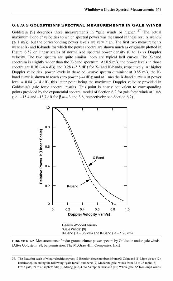
Windblown Clutter Spectral Measurements 669

6.6.3.5 Goldstein’s Spectral Measurements in Gale Winds

Goldstein [9] describes three measurements in “gale winds or higher.”37 The actualmaximum Doppler velocities to which spectral power was measured in these results are low(≤ 1 m/s), but the corresponding power levels are very high. The first two measurementswere at X- and K-bands for which the power spectra are shown much as originally plotted inFigure 6.57 on linear scales of normalized spectral power density (0 to 1) vs Dopplervelocity. The two spectra are quite similar; both are typical bell curves. The X-bandspectrum is slightly wider than the K-band spectrum. At 0.5 m/s, the power levels in thosespectra are 0.36 (–4.4 dB) and 0.28 (–5.5 dB) for X- and K-bands, respectively. At higherDoppler velocities, power levels in these bell-curve spectra diminish: at 0.85 m/s, the K-band curve is shown to reach zero power (–∞ dB); and at 1 m/s the X-band curve is at powerlevel = 0.04 (–14 dB), this latter point being the maximum Doppler velocity provided inGoldstein’s gale force spectral results. This point is nearly equivalent to correspondingpoints provided by the exponential spectral model of Section 6.2 for gale force winds at 1 m/s(i.e., –15.4 and –13.7 dB for β = 4.3 and 3.8, respectively; see Section 6.2).

37. The Beaufort scale of wind velocities covers 13 Beaufort force numbers [from (0) Calm and (1) Light air to (12) Hurricane], including the following “gale force” numbers: (7) Moderate gale, winds from 32 to 38 mph; (8) Fresh gale, 39 to 46 mph winds; (9) Strong gale, 47 to 54 mph winds; and (10) Whole gale, 55 to 63 mph winds.

Figure 6.57 Measurements of radar ground clutter power spectra by Goldstein under gale winds. (After Goldstein [9]; by permission, The McGraw-Hill Companies, Inc.)

0 0.2 0.4 0.8

0

0.2

0.4

0.8

1.0

Doppler Velocity v (m/s)

Rel

ativ

e P

ow

er k

(L

inea

r S

cale

)

X-Band

0.6

1.00.6

K-Band

Heavily Wooded Terrain“Gale Winds” [9]X-Band ( = 3.2 cm) and K-Band ( = 1.25 cm) λ λ

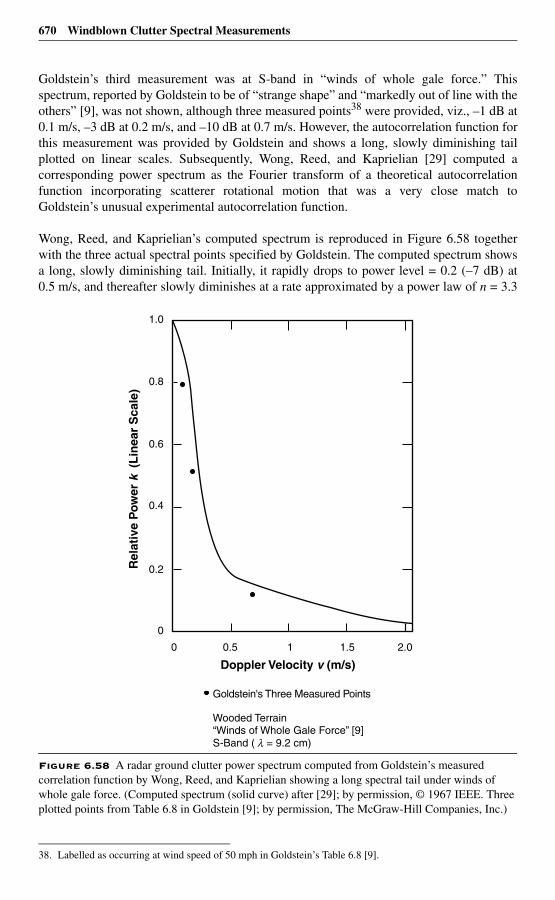
670 Windblown Clutter Spectral Measurements

Goldstein’s third measurement was at S-band in “winds of whole gale force.” Thisspectrum, reported by Goldstein to be of “strange shape” and “markedly out of line with theothers” [9], was not shown, although three measured points38 were provided, viz., –1 dB at0.1 m/s, –3 dB at 0.2 m/s, and –10 dB at 0.7 m/s. However, the autocorrelation function forthis measurement was provided by Goldstein and shows a long, slowly diminishing tailplotted on linear scales. Subsequently, Wong, Reed, and Kaprielian [29] computed acorresponding power spectrum as the Fourier transform of a theoretical autocorrelationfunction incorporating scatterer rotational motion that was a very close match toGoldstein’s unusual experimental autocorrelation function.

Wong, Reed, and Kaprielian’s computed spectrum is reproduced in Figure 6.58 togetherwith the three actual spectral points specified by Goldstein. The computed spectrum showsa long, slowly diminishing tail. Initially, it rapidly drops to power level = 0.2 (–7 dB) at0.5 m/s, and thereafter slowly diminishes at a rate approximated by a power law of n = 3.3

38. Labelled as occurring at wind speed of 50 mph in Goldstein’s Table 6.8 [9].

Figure 6.58 A radar ground clutter power spectrum computed from Goldstein’s measured correlation function by Wong, Reed, and Kaprielian showing a long spectral tail under winds of whole gale force. (Computed spectrum (solid curve) after [29]; by permission, © 1967 IEEE. Three plotted points from Table 6.8 in Goldstein [9]; by permission, The McGraw-Hill Companies, Inc.)

Doppler Velocity v (m/s)

Rel

ativ

e P

ow

er k

(L

inea

r S

cale

)

1.0

0 1

Goldstein's Three Measured Points

0.8

0.6

0.4

0.2

0

2.0

“Winds of Whole Gale Force” [9]Wooded Terrain

S-Band ( = 9.2 cm) λ

1.50.5

Windblown Clutter Spectral Measurements 671

to power level = 0.02 (–17 dB) at 2 m/s. In comparison, at 2 m/s the widest measured LCEspectrum is at –53 dB. In discussing these curves of correlation function and powerspectrum, Wong, Reed, and Kaprielian noted that they “deviate significantly from the usualexpected Gaussian shape. Instead, they drop very slowly toward zero” [29]. Thus these datahave contributed to the concept of a long spectral tail, here at an usually high power level.

Some reservations must be accorded to Goldstein’s results, due to their very early origin.Goldstein was attempting to establish only the most basic general characteristics and,indeed, just the very existence of spectral spreading of ground clutter in these early results.Conversion of values from near the limits of Goldstein’s plots on linear scales to decibelquantities for comparison with modern measurements to much lower power levels wherethe concern is with detailed behavior of spectral tails is using Goldstein’s data out ofhistorical context. In particular, Goldstein’s unusual S-band gale force data and their furtherelaboration by Wong, Reed, and Kaprielian [29] now appear to be best regarded as ananomalous occurrence in an isolated measurement. No modern measurements ofwindblown tree clutter spectra under gale force winds are known to exist.

6.6.3.6 Armand’s Long, Low-Level Clutter Spectral Tail

Armand et al. [14] ostensibly measured X-band clutter spectra from windblown trees tovery low levels of spectral power (–120 dB) and correspondingly very high Dopplervelocities (20 m/s). Their results are reproduced in Figure 6.59. Armand et al. stated thatthese ground clutter spectra were measured with CW equipment in which the powerreceived from the sidelobes of the transmitter was an order of magnitude higher than thatreflected from the trees. Instabilities were reported to be eliminated through use ofklystrons stabilized by cooling with liquid helium. Results were obtained in the 40- to2,500- Hz Doppler frequency band (i.e., not near the carrier). Spectral results are shown forthree wind speeds—4, 13, and 31 mph—over the range from 40 to ∼ 1,300 Hz (0.6 to∼ 20 m/s). Over this range, the spectral power density levels are between –50 and –120 dB(i.e., are much lower than any other known spectral measurements).

For the 4-mph spectrum, the power drops to –120 dB at 2.5 m/s, and thereafter stays at ∼ –120dB all the way out to 20 m/s (i.e., exhibits a long spectral tail at a uniform low level, likeWhite’s [39] conceptual wideband noise-like spectral component). The 13- and 31-mphspectra drop gradually from –63 and –52 dB, respectively, at 0.6 m/s to ∼ –115 dB at 20 m/s.At power levels 80 dB down, Doppler velocities in the Armand et al. results of Figure 6.59 are∼ 0.9, 1.4, and 2.5 m/s for 4-, 13-, and 31-mph winds, respectively; these spectral widths are avery close match to those measured by Phase One and LCE at similar levels of spectral power(i.e., near their limits of sensitivity).

Armand et al. [14] claimed that their spectral shapes were power-law, with an average valueof power-law exponent n = 3 in the 110- to 2,500-Hz band averaged over all tests and withn varying inversely with wind velocity between 3 and 6 in the 40- to 110-Hz band. Theauthenticity of these very long, very low-level clutter spectral tails is open to question; whatwas measured may have been effects of sidelobes, internal system instabilities, etc. Beforeundue credibility is ascribed to these results, they need to be confirmed by independent andconsistent replication using modern measurement instrumentation. However, these resultsarguably keep open the possibility of long spectral tails at very low power levels belowPhase One and LCE sensitivities. As previously discussed, spectral power at large Dopplervelocities is theoretically accounted for by Armand et al. through amplitude modulation via

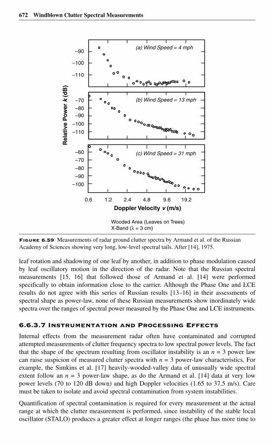
672 Windblown Clutter Spectral Measurements

leaf rotation and shadowing of one leaf by another, in addition to phase modulation causedby leaf oscillatory motion in the direction of the radar. Note that the Russian spectralmeasurements [15, 16] that followed those of Armand et al. [14] were performedspecifically to obtain information close to the carrier. Although the Phase One and LCEresults do not agree with this series of Russian results [13–16] in their assessments ofspectral shape as power-law, none of these Russian measurements show inordinately widespectra over the ranges of spectral power measured by the Phase One and LCE instruments.

6.6.3.7 Instrumentation and Processing Effects

Internal effects from the measurement radar often have contaminated and corruptedattempted measurements of clutter frequency spectra to low spectral power levels. The factthat the shape of the spectrum resulting from oscillator instability is an n = 3 power lawcan raise suspicion of measured clutter spectra with n = 3 power-law characteristics. Forexample, the Simkins et al. [17] heavily-wooded-valley data of unusually wide spectralextent follow an n = 3 power-law shape, as do the Armand et al. [14] data at very lowpower levels (70 to 120 dB down) and high Doppler velocities (1.65 to 37.5 m/s). Caremust be taken to isolate and avoid spectral contamination from system instabilities.

Quantification of spectral contamination is required for every measurement at the actualrange at which the clutter measurement is performed, since instability of the stable localoscillator (STALO) produces a greater effect at longer ranges (the phase has more time to

Figure 6.59 Measurements of radar ground clutter spectra by Armand et al. of the Russian Academy of Sciences showing very long, low-level spectral tails. After [14], 1975.

0.6 1.2 2.4 4.8 9.6 19.2

–90

–100

–110

(a) Wind Speed = 4 mph

(b) Wind Speed = 13 mph

Doppler Velocity v (m/s)

(c) Wind Speed = 31 mph

Rel

ativ

e P

ower

k (

dB

)

–90

–80

–100

–70

–60

–100

–90

–110

–80

–70

Wooded Area (Leaves on Trees)X-Band (λ = 3 cm)

Windblown Clutter Spectral Measurements 673

change when the STALO is used to upconvert on transmit and downconvert on receive). Ifthe STALO is not used on receive, but the signal is merely envelope-detected prior tospectral analysis (as in the results of Goldstein [9] and Fishbein et al. [10]), the fullSTALO instability spectrum or that of the transmitter is impressed on the received cluttersignal. Goldstein’s [9] early measurements were undoubtedly made using a klystron ormagnetron as the transmitter, resulting in relatively poor stability.

In the Armand et al. [14] results, transitions are observable in the spectral data at lowpower levels (at 1.5 m/s Doppler velocity for 4-mph wind speed, and at 2.4 m/s Dopplervelocity for 13-mph wind speed). For Doppler velocities greater than those of thesetransition points, it is conceivable that the data result from system instabilities. Note thatthe results of Armand et al. were obtained using a CW transmitter; use of pulsed radar canintroduce additional instability due to noise contamination of trigger pulses. Nonlinearitiesin circuitry or processing (e.g., lin-limit amplifier) can also limit and spread the frequencyspectrum, especially under strong signal (strong clutter) conditions. Data in saturationresult in significant spectral spreading caused by the actual spectrum convolving withitself in such circumstances. Discounting this possibility for the stationary false alarmcells underlying the Simkins et al. heavily-wooded-valley data is the reported fact thatspectra from adjacent non-false alarm cells of similar intensity were narrower. Unwantedantenna motion caused mechanically, and/or by the wind, can also spread the frequencyspectrum by modulating the clutter signal. This modulation may go unobserved if stabilitytesting is performed in low-wind conditions.

A few cases of long spectral tails extending to Doppler velocities >> 3 m/s were observedduring the course of examining the Phase One database of spectral measurements. In everycase, the long spectral tail was isolated to some sort of instrumentation problem (e.g.,sticking bits on the A/D converter generating minute sample-and-hold stairsteps on thetemporal signal, occasional saturations, external interference). One excessively wide PhaseOne spectral measurement caused by undetected saturation was inadvertently included in aset of “windy” spectra in a previous publication (spectrum 4, Figure 6.9, in [21]). Thus anyunusually wide measured spectra should always be very carefully examined in the timedomain before accepting the wide frequency domain result.

Attempts to improve Phase One stability by sampling the transmitted signal and correcting(i.e., subtracting) transmitted phase variations in the received signal were unsuccessful (i.e.,proved to be not simple to implement). The LCE radar was a spectrally purer system thanthe Phase One radar and was never observed to generate an excessively wide spectral taildue to system or processing contamination. A number of windblown clutter spectralmeasurements by other investigators reviewed from time to time by the author have at firstcontained obviously corrupted clutter spectral tails of excessive width and extremely slow(e.g., n ≅ 3) decay; subsequent investigation has always found these long spectral tails tobe caused by errors in instrumentation or processing. In considering all the possible ways inwhich instrumentation limitations or processing errors can broaden measured clutterspectra, it is well to bear in mind that of two measured spectra—one narrow and onewide—ostensibly characterizing the same clutter phenomenon, the narrower spectrum isalways more credible since all corruptive influences due to instrumentation limitations orprocessing errors can only broaden the spectrum, not narrow it.

Because of all the potential uncertainties (i.e., potential contaminants of internal andexternal origin) in radar ground clutter spectral measurements as exemplified in the

674 Windblown Clutter Spectral Measurements

preceding discussions of Section 6.6.3, the use of such data requires the exercise ofjudgment. Ground clutter spectral models should reflect, for the most part, centralrepeatable trends in measured data, not unusual or isolated artifacts or aberrations.

6.7 SummaryAccurate characterization of radar ground clutter spectral shape is important in radartechnology applications in which target signals compete with strong ground clutterreturns. Ground clutter spectral spreading can limit the performance of MTI/Dopplerprocessors, including both conventional one-dimensional fixed-parameter designs [1, 2]and modern two-dimensional displaced phase-centered antenna or space-time adaptivetechniques [3–5] for detecting and tracking moving targets in clutter backgrounds. Internalclutter motion can also cause defocusing in SAR processing [62] and indeed can degradeany radar processing technique that assumes the clutter to be stationary. Such reasonsprovide motivation to obtain a proper understanding of clutter spectral spreading and toobtain an accurate characterization of the shapes of clutter spectra to very low levels ofspectral power. Historically, the state of knowledge of windblown ground clutter spectralshape has been rather poor, and considerable disagreement has existed concerning theextent to which Doppler spreading occurs in such spectra.

Lincoln Laboratory measurement data indicate that ground clutter power spectra overspectral dynamic ranges reaching 60 to 80 dB below the zero-Doppler peaks are relativelynarrow and reasonably characterized as of exponential shape. First observation ofexponential spectral decay in the clutter studies discussed herein occurred in the earlyexamination of windblown foliage clutter spectra obtained with the Phase One cluttermeasurement radar at western Canadian sites. These first observations of exponential decayremained valid in the general representation of a much more complete set of L-bandspectral measurements over various regimes of wind speed obtained with the Phase Oneradar at the Lincoln Laboratory measurement site of Katahdin Hill in easternMassachusetts [21].

Exponential decay was also concluded to be the best overall characterization of windblownground clutter spectral shape covering Phase One measurements at other frequencies (i.e.,VHF, UHF, S-, and X-bands), from other sites, and over several thousand spectralobservations taken from the extensive L-band database of clutter spectral measurementssubsequently obtained with the LCE clutter measurement radar [25]. The LCE radar was amajor L-band-only upgrade of the five-frequency Phase One radar with new, muchimproved receiver and data recording units, lower phase noise levels, and very clean andreliable spectral response. Analyses of Phase One clutter data in Canada [22, 23] and in theU. K. [24] also concluded that ground clutter spectra were generally best-fitted withexponential shapes.

On the basis of the Phase One and LCE clutter data, two different first-principlestheoretical models [39, 60] were independently developed for the windblown clutterDoppler spectrum that, although mathematically complex, in both cases provide close toexponential decay under numerical evaluation. Other previous references to exponential (orquasi- or partially-exponential) clutter spectral decay exist in a much earlier LincolnLaboratory measurement program [59] of the 1970s, and in Russian measurements [13–16]and French measurements [38] of the same early time period.

Windblown Clutter Spectral Measurements 675

The very earliest indications were that windblown ground clutter spectra were of Gaussianspectral shape [6–9]. Many subsequent measurements to lower power levels 30 to 40 dBbelow the peak zero-Doppler level indicated spectral shapes that were significantly widerthan Gaussian in their tails and that appeared to be well approximated with power-lawfunctions [10–20]. The Phase One and LCE ground clutter spectral measurements, over suchlimited spectral dynamic ranges, also can be adequately modeled as of power-law shapes.However, the Phase One and LCE measurement data also clearly indicate that the power-lawrates of decay at upper levels of spectral power do not continue to lower levels of spectralpower reaching 60 to 80 dB down from the zero-Doppler peak. The measured power-lawrates of decay at lower power levels are always much faster than at the upper levels.

An exponential representation generally captures, at least approximately and occasionallyhighly accurately, the major attributes of the windblown clutter ac spectral shape functionover the entire range from near the zero-Doppler peak to measured levels 60 to 80 dBdown. In contrast, the windblown clutter ac spectral shape is not at all representable by anypower law over such a wide spectral dynamic range. The maximum Phase One- and LCE-measured Doppler velocity spectral extents from windblown foliage at levels 60 to 80 dBdown are ≈3 to 4 m/s. Power-law models can extrapolate data of 40-dB spectral dynamicrange to spectral extent as great as 30 m/s, 60 dB down. Such extreme windblown foliagespectral extents have never been corroborated by any results in the extensive Phase One andLCE databases of windblown clutter spectral measurements.

Chapter 6 provides a new empirical model for windblown ground clutter Doppler spectrabased on many clutter spectral measurements obtained with the Lincoln Laboratory LCEand Phase One five-frequency (VHF, UHF, L-, S-, and X-band) radars. This model iscomplete, including both ac and dc components of the spectrum. The important parametersincorporated in the model are wind speed and radar carrier frequency. Ac spectral shape isspecified as exponential, with the Doppler-velocity exponential shape factor stronglydependent on wind speed but independent of radar frequency, VHF to X-band. The fact thatac spectral spreading occurs at VHF in windblown clutter Doppler-velocity spectra more orless equivalently as at X-band is illustrated through representative measurement results;many other examples of VHF-measured clutter spectra with similar spectral spreading existin the Phase One and LCE databases.

The major difference between VHF and X-band clutter spectra is that a much larger dcspectral component exists at VHF compared with X-band. The ratio of dc to ac spectralpower in the model is determined by an analytic expression empirically derived from themeasurements that captures the strong dependencies of dc/ac ratio on both wind speed andradar frequency. Chapter 6 includes both a complete specification of the clutter spectralmodel and a thorough comparison of model predictions with many examples of measuredwindblown clutter spectra under various combinations of radar parameters andmeasurement circumstances. Besides wind speed and radar frequency, other parametersthat might be thought to significantly influence clutter spectra, but that appear to be largelysubsumed within general ranges of statistical variability in the measurement data, includetree species, season of the year, wind direction, cell size, polarization, range, and grazingangle. The exponential model is explicitly derived to be applicable to windblown trees, butexamples are also provided of measured clutter spectra from scrub desert, cropland, andrangeland that indicate the model can also perform adequately for other windblownvegetation types by suitably adjusting its dc/ac term.

676 Windblown Clutter Spectral Measurements

Although it is now generally accepted that radar ground clutter spectral shapes are wider thanGaussian in their tails, the simple Gaussian continues to be how clutter spectra are usuallyrepresented in radar system engineering (at least as a method of first approach in representingeffects of intrinsic clutter motion) because of its simplicity and analytic tractability. TheGaussian spectral shape is theoretically generated by a group of moving scatterers, each ofrandom translational drift velocity [19]. Theory also suggests that the origin of the increasedspreading observed in measured ground clutter spectra beyond that predicted by Gaussian islargely due to the random oscillatory motion of leaves and branches, in contrast to simplerandom translational motion [19, 29, 42]. Like the Gaussian spectral shape, the exponentialspectral shape is also simple and analytically tractable and has the advantage of being widerthan Gaussian as required by experiment and supported by theory.

There is no underlying fundamental physical principle requiring clutter spectra to beprecisely of exponential shape. Many of the Phase One and LCE clutter spectralmeasurements, particularly many of the narrower spectra occurring at lower wind speeds,are less exponential overall than some of the wider measured spectra. To be clear on thismatter, almost none of the Phase One- and LCE-measured clutter spectra can be accuratelyrepresented by any single simple analytic function, including exponential [31], over theircomplete spectral dynamic ranges, from the point of view of passing rigorous statisticalhypothesis tests. Use of the exponential shape in Chapter 6 is as a convenient analyticbounding envelope that empirically approximates, occasionally very accurately, many ofthe LCE and Phase One measurements over most of their spectral dynamic ranges,including the lowest power levels measured. The resulting model overcomes much of thedifficulty in modeling clutter spectra not only by using exponential shapes, but also byintroducing the concept of a quasi-dc region and absorbing the excess power measured inthe quasi-dc region into the dc delta function term of the model. This approach allows themodel the flexibility of using the exponential representation to optimally match themeasured spectral spreading in the spectral tail regions without regard to the narrow near-zero-Doppler quasi-dc region, which often displays a different rate of decay than occurs inthe broad spectral tail [31].

In addition to showing that measured shapes of windblown ground clutter Doppler spectraappear to be much more closely matched by an exponential approximation than byGaussian (too narrow) or power-law (too wide) approximations, Chapter 6 also investigatesthe impact of assigning the correct clutter spectral shape on MTI and STAP coherent targetdetection. Compared to the exponential shape, the Gaussian shape substantiallyunderpredicts the effects of clutter on detection, and the power-law shape substantiallyoverpredicts the effects of clutter on detection. The exponential spectral model forwindblown foliage is validated by showing that the differences in clutter improvementfactor performance prediction between using actual measured I/Q data as input to theclutter canceller, and modeled clutter data of Gaussian, exponential, or power-law spectralshape, are minimized when the spectral model employed is of exponential shape.

It is evident on the basis of the Phase One and LCE measurements that the current state ofknowledge regarding the extent of spectral spreading in windblown ground clutter has beenadvanced to the point where it is relatively incontrovertible that clutter spectra fromwindblown vegetation, although wider than Gaussian, are still generally relatively narrowand spread to Doppler velocities < ≈3 or 4 m/s over spectral power levels reaching to 80dB below zero-Doppler peaks for wind speeds in the 15- to 30-mph range. Investigators

Windblown Clutter Spectral Measurements 677

who may wish to continue to argue for much wider clutter spectra from windblown foliageover such ranges are faced with proving spectral purity in their wider measurements, sinceunknown corruptive instrumentation or processing effects can only widen spectra, notnarrow them. Presumably, most of the spectral spreading that occurs in the Phase One andLCE data is caused by the velocity distribution (translational and/or oscillatory) of thefoliage, that is, by the radial motion of individual scatterers (leaves and branches) towardand away from the radar causing phase modulation in the returned signal. To whateverextent other effects are also at work in the Phase One and LCE data, such as leaf rotation orthe shadowing of one leaf by another causing more complex amplitude modulation effects,such effects are also constrained to cause limited spreading to levels 80 dB down.

Chapter 6 also provides a relatively thorough review of the available literature of clutterspectral measurements, which generally brings it and the Phase One and LCE results intoconformity and agreement. There remain hints in the literature, however, not only fromtheoretical reasoning but also in various poorly substantiated measurement results, of longspectral tails existing in ground clutter data to Doppler velocities greatly exceeding themaximum ≈3 to 4 m/s observed in the Phase One and LCE data. Arguments for theexistence of such wide tails often are based on postulated leaf-rotation and leaf-shadowingeffects. Such long tails have never been observed, whether as slowly decaying power lawsor as uniform-amplitude wideband noise-like components, in any of the several thousandspectra that have been examined from the extensive Phase One and LCE databases ofground clutter spectral measurements to levels reaching 60 to 80 dB below zero-Dopplerpeaks. What might occur at lower levels remains conjectural.

References1. M. I. Skolnik, Introduction to Radar Systems, 3rd ed., New York: McGraw-Hill

(2001).

2. J. A. Scheer and J. L. Kurtz (eds.), Coherent Radar Performance Estimation, Boston,MA: Artech House, Inc. (1993).

3. R. Klemm, Space-Time Adaptive Processing: Principles and Applications, IEEPress, Radar, Sonar, Navigation and Avionics Series, 1999.

4. J. Ward, “Space-Time Adaptive Processing for Airborne Radar,” Lexington, MA:MIT Lincoln Laboratory, Technical Rep. 1015 (13 December 1994), DTIC AD-A293032.

5. P. Richardson, “Relationships between DPCA and adaptive space-time processingtechniques for clutter suppression,” Proc. International Conf. Radar, SEE 48 rue dela Procession, 75724 Paris Cedex 15 (May 1994), pp. 295–300.

6. L. N. Ridenour (ed.), Radar System Engineering, Vol. 1 in the MIT RadiationLaboratory Series, New York: McGraw-Hill (1947). Reprinted, Dover Publications(1965).

7. E. J. Barlow, “Doppler Radar,” Proc. IRE 37, 4 (1949).

8. J. L. Lawson and G. E. Uhlenbeck (eds.), Threshold Signals, Vol. 24 in the MITRadiation Laboratory Series, New York: McGraw-Hill (1950).

678 Windblown Clutter Spectral Measurements

9. H. Goldstein, “The Fluctuations of Clutter Echoes,” pp. 550–587, in D. E. Kerr (ed.),Propagation of Short Radio Waves, Vol. 13 in the MIT Radiation Laboratory Series,New York: McGraw-Hill (1951).

10. W. Fishbein, S. W. Graveline, and O. E. Rittenbach. “Clutter Attenuation Analysis,”Fort Monmouth, NJ: U.S. Army Electronics Command, Technical Rep. ECOM-2808(March 1967). Reprinted in MTI Radar, D.C. Schleher (ed.), Boston, MA: ArtechHouse, Inc. (1978).

11. M. P. Warden and B. A. Wyndham, “A Study of Ground Clutter Using a 10-cmSurveillance Radar,” Royal Radar Establishment, Technical Note No. 745, Malvern,U. K. (1969). DTIC AD 704874.

12. N. C. Currie, F. B. Dyer, and R. D. Hayes, “Radar Land Clutter Measurements atFrequencies of 9.5, 16, 35, and 95 GHz,” Engineering Experiment Station, GeorgiaInstitute of Technology, Technical Report No. 3, United States Army, ContractDAAA-25-73-C-0256, April 1975. DTIC AD-A012709.

13. V. A. Kapitanov, V. Mel’nichuk, and A. A. Chernikov, “Spectra of radar signalsreflected from forests at centimeter waves,” Radio Eng. and Electron. Phys., 18, 9(1973).

14. N. A. Armand, V. A. Dyakin, I. N. Kibardina, A. G. Pavel’ev, and V. D. Shuba, “Thechange in the spectrum of a monochromatic wave when reflected from movingscatterers,” Radio Eng. and Electron. Phys., 20, 7 (1975).

15. V. A. Andrianov, I. S. Bondarenko, I. N. Kibardina, V. K. Prosshin, and D. Y. Shtern,“Characteristics of measurement of spectra of radio signals scattered by anunderlying surface,” Radio Eng. and Electron. Phys., 21, 2 (1976).

16. V. A. Andrianov, N. A. Armand, and I. M. Kibardina, “Scattering of radio waves byan underlying surface covered with vegetation,” Radio Eng. and Electron. Phys., 21,9 (1976).

17. W. L. Simkins, V. C. Vannicola, and J. P. Ryan, “Seek Igloo Radar Clutter Study,”Rome Air Development Center, Technical Rep. RADC-TR-77-338 (October 1977).Updated in FAA-E-2763b Specification, Appendix A (May 1988). See also FAA-E-2763a (September 1987), FAA-E-2763 (January 1986, July 1985).

18. J. Jiankang, Z. Zhongzhi, and S. Zhong, “Backscattering power spectrum forrandomly moving vegetation,” Proc. IGARSS Symposium, Zurich (August 1986),pp. 1129–1132.

19. N. J. Li, “A study of land clutter spectrum,” Proc. 1989 International Symp. on Noiseand Clutter Rejection in Radars and Imaging Sensors, T. Suzuki, H. Ogura, andS. Fujimura (eds.), IEICE, Kyoto (1989), pp. 48–53.

20. G. W. Ewell, private communication (December 1995).

21. J. B. Billingsley and J. F. Larrabee, “Measured Spectral Extent of L- and X-BandRadar Reflections from Windblown Trees,” Lexington, MA: MIT LincolnLaboratory, Project Rep. CMT-57 (6 February 1987), DTIC AD-A179942.

22. H. C. Chan, “Spectral Characteristics of Low-Angle Radar Ground Clutter,” Ottawa,Canada: Defence Research Establishment Ottawa, Report No. 1020 (December1989), DTIC AD-A220817.

Windblown Clutter Spectral Measurements 679

23. H. C. Chan, “Radar ground clutter measurements and models, part 2: Spectralcharacteristics and temporal statistics,” AGARD Conf. Proc. Target and ClutterScattering and Their Effects on Military Radar Performance, Ottawa, AGARD-CP-501 (1991), AD-P006374.

24. G. C. Sarno, “A model of coherent radar land backscatter,” AGARD Conf. Proc.Target and Clutter Scattering and Their Effects on Military Radar Performance,Ottawa, AGARD-CP-501 (1991), AD-P006375.

25. J. B. Billingsley, “Exponential Decay in Windblown Radar Ground Clutter DopplerSpectra: Multifrequency Measurements and Model,” Lexington, MA: MIT LincolnLaboratory, Technical Report 997, 29 July 1996; DTIC AD-A312399.

26. J. B. Billingsley, “Windblown radar ground clutter Doppler spectra: measurementsand model,” submitted to IEEE Trans. AES, May 2000, accepted subject to minorrevision, October 2000.

27. M. W. Long, Radar Reflectivity of Land and Sea, 3rd ed., Boston: Artech House, Inc.(2001).

28. F. E. Nathanson, Radar Design Principles, 2nd ed., New York: McGraw-Hill (1991).Reprinted, SciTech Publishing, Inc., 1999.

29. J. L. Wong, I. S. Reed, and Z. A. Kaprielian, “A model for the radar echo from arandom collection of rotating dipole scatterers,” IEEE Trans. AES 3, 2 (1967).

30. M. V. Greco, F. Gini, A. Farina, and J. B. Billingsley, “Analysis of cluttercancellation in the presence of measured L-band radar ground clutter data,” inProceedings of IEEE International Radar Conference (Radar 2000), Alexandria,VA, May 8–12, 2000.

31. M. V. Greco, F. Gini, A. Farina, and J. B. Billingsley, “Validation of windblown radarground clutter spectral shape,” IEEE Trans. AES, vol. 37, no. 2, April 2001.

32. J. B. Billingsley, A. Farina, F. Gini, M. V. Greco, and P. Lombardo, “Impact ofexperimentally measured Doppler spectrum of ground clutter on MTI and STAP,” inProceedings of IEE International Radar Conference (Radar ‘97), IEE Conf. Pub.No. 449, pp. 290-294, Edinburgh, 14–16 October 1997.

33. P. Lombardo, M. V. Greco, F. Gini, A. Farina, and J. B. Billingsley, “Impact of clutterspectra on radar performance prediction,” IEEE Trans. AES, vol. 37, no. 3, July2001.

34. J. B. Billingsley and J. F. Larrabee, “Bragg Resonance in Measured L-band RadarClutter Doppler Spectra from Inland Water,” Lexington, MA: MIT LincolnLaboratory, Technical Rep. 1019 (1 August 1995), DTIC AD-A297680.

35. J. B. Billingsley, “Measurements of L-band inland-water surface-clutter Dopplerspectra,” IEEE Trans AES, Vol. 34, No. 2, April 1998, pp. 378–390.

36. R. L. Ferranti, “Very low phase noise in a pulsed 10-kw L-band triode poweramplifier,” Santa Clara, CA: Proc. RF Expo West, 59-66 (February 1991).

37. F. J. Harris, “On the use of windows for harmonic analysis with the discrete Fouriertransform,” Proc. IEEE 66, 51–83 (January 1978).

680 Windblown Clutter Spectral Measurements

38. R. Basard, “Vegetation clutter Doppler spectrum models,” International Conferenceon Radar, (Session II), Paris, pp. 28-31, 4–8 December 1978.

39. R. G. White, “A model for MTI radar clutter,” Proc. SEE Int. Radar Conf., Paris(May 1994), pp. 540–545.

40. R. M. Narayanan, D. W. Doerr, and D. C. Rundquist, “Temporal decorrelation of X-band backscatter from wind-influenced vegetation,” IEEE Trans. Aerosp. Electron.Syst. 28, 2 (1992), pp. 404–412.

41. R. M. Narayanan, S. E. Nelson, and J. P. Dalton, “Azimuthal scattering pattern oftrees at X-band,” IEEE Trans. Aerosp. Electron. Syst. 29, 2 (1993), pp. 588–593.

42. R. M. Narayanan, D. W. Doerr, and D. C. Rundquist, “Power spectrum of wind-influenced vegetation backscatter at X-band,” IEE Proc.-Radar, Sonar Navig., 141, 2(1994), pp. 125–131.

43. N. A. Stewart, “Use of crosspolar returns to enhance target detectability,” in J. Clarke(ed.), Advances in Radar Techniques, IEE Electromagnetic Wave Series 20, PeterPeregrinus, Ltd., London, U.K., 1985, pp. 449–454.

44. J. B. Billingsley and J. F. Larrabee, “Multifrequency Measurements of Radar GroundClutter at 42 Sites,” Lexington, MA: MIT Lincoln Laboratory, Technical Rep. 916,Volumes 1, 2, 3 (15 November 1991), DTIC AD-A246710.

45. G. P. de Loor, A. A. Jurriens, and H. Gravesteijn, “The radar backscatter fromselected agricultural crops,” IEEE Trans. on Geoscience Electronics, 12, 70–77(April 1974).

46. E. J. Kelly, “An adaptive detection algorithm,” IEEE Trans. on Aerospace andElectronic Systems, Vol. 22, No. 2, pp. 115–127, March 1986.

47. A. Farina, P. Lombardo, M. Pirri, “Non-linear space-time processing for airborneearly warning radar,” IEE Proc. on Radar, Sonar and Navigation, Vol. 145, No. 1,pp. 9–18, February 1998.

48. R. Klemm, “Adaptive clutter suppression for airborne phased-array radars,” IEEProceedings-F, Vol. 130, No. 1, pp. 125–132, February 1983.

49. S. Barbarossa and A. Farina, “Space-time-frequency processing of synthetic apertureradar signals,” IEEE Trans. on Aerospace and Electronic Systems, Vol. 30, No. 2, pp.341–358, April 1994.

50. D. K. Barton, Modern Radar System Analysis, Boston, MA: Artech House, Inc.(1988), p. 246.

51. A. Papoulis, The Fourier Integral and Its Applications, New York: McGraw-Hill(1962).

52. W. B. Davenport, Jr., and W. L. Root, An Introduction to the Theory of RandomSignals and Noise, New York: McGraw-Hill (1958).

53. S. Goldman, Frequency Analysis, Modulation, and Noise, New York: McGraw-Hill(1948). Reprinted, Dover Publications (1967).

Windblown Clutter Spectral Measurements 681

54. F. G. Bass, P. V. Bliokh, and I. M. Fuks, “Statistical characteristics of a signalscattered from randomly moving reradiators on a plane section,” translated fromRadiotechnika i Electronika (USSR), 10, 5 (May 1965), pp. 731–739.

55. S. Rosenbaum and L.W. Bowles, “Clutter return from vegetated areas,” IEEE Trans.Ant. Propag., AP-22, 2 (March 1974), pp. 227–236.

56. D. C. Schleher, MTI and Pulsed Doppler Radar, Norwood, MA: Artech House,1991, p. 127.

57. J. A. Scheer, “Coherent Radar Performance Estimation,” IEEE National RadarConference, Tutorial Notes, Atlanta (1994).

58. N. C. Currie and C. E. Brown, eds., Principles and Applications of Millimeter-WaveRadar, Norwood, MA: Artech House, Inc. (1987).

59. L. Cartledge, M. Labitt, J. H. Teele, and R. D. Yates, “An Experimental UHF GroundSurveillance Radar, Volume 2,” Lexington, MA: MIT Lincoln Laboratory, TechnicalRep. 497 (12 October 1972), DTIC AD-757565.

60. P. Lombardo and J. B. Billingsley, “A new model for the Doppler spectrum ofwindblown radar ground clutter,” in Proceedings of 1999 IEEE Radar Conference,Boston, MA, 20-22 April 1999, pp. 142–147.

61. R. G. White, private communication (11 September 1995).

62. C. Elachi and D. D. Evans “Effects of random phase changes on the formation ofsynthetic aperture radar imagery,” IEEE Trans. on Antennas and Propagation, Vol.AP-25, No. 1, pp. 149–153, January 1977.

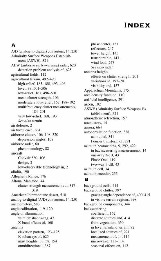
Index

AA/D (analog-to-digital) converters, 14, 250Admiralty Surface Weapons Establish-

ment (ASWE), 321AEW (airborne early-warning) radar, 620

detection problem analysis of, 625agricultural fields, 112agricultural terrain, 492–493

high-relief, 185–188, 493–496level, 88, 501–506low-relief, 167, 496–501mean clutter strength, 106moderately low-relief, 167, 188–192multifrequency clutter measurements,

184–201very low-relief, 168, 193See also terrain

air defense, 2air turbulence, 664airborne clutter, 106–108, 320

depression angles, 108airborne radar, 60

phenomenology, 82aircraft

Convair 580, 106design, 2low-observable technology in, 2

alfalfa, 190Allegheny Range, 176Altona, Manitoba, 44

clutter strength measurements at, 317–319

American Intermontane desert, 510analog-to-digital (A/D) converters, 14, 250anemometers, 583angle calibration, 119–120angle of illumination

vs microshadowing, 43X-band effects of, 160

antennaelevation pattern, 123–125K subarrays of, 625mast heights, 38, 58, 154omnidirectional, 387

phase center, 123reflectors, 247tower height, 145transportable, 143wind load, 247See also radar

antenna heightseffects on clutter strength, 201variations in, 197–201visibility and, 157

Appalachian Mountains, 175area density function, 110artificial intelligence, 291aspen, 182ASWE (Admiralty Surface Weapons Es-

tablishment), 321atmospheric refraction, 157attenuators, 14aurora, 664autocorrelation function, 338

azimuthal, 341Fourier transform of, 291

azimuth beamwidths, 9, 292, 422in backscattering measurements, 14one-way 3-dB, 43Phase One, 419two-way 3-dB, 43

azimuth cell, 341azimuth encoder, 255

Bbackground cells, 414background clutter, 397

grazing angle dependence of, 400, 415in visible terrain regions, 398

background components, 344backscattering

coefficient, 162discrete sources and, 414from vegetation, 650in level farmland terrain, 92localized sources of, 221measurement of, 14, 115microwave, 111–114seasonal effects on, 112

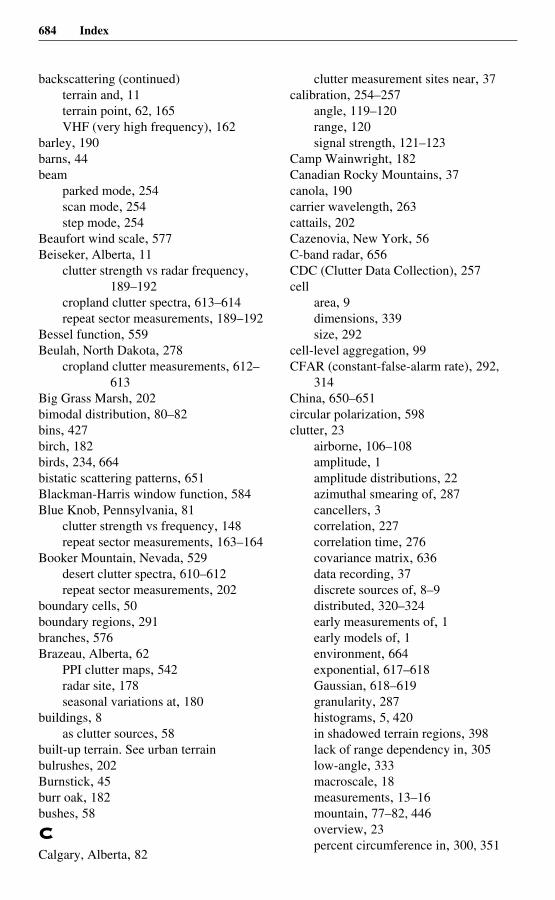
684 Index

backscattering (continued)terrain and, 11terrain point, 62, 165VHF (very high frequency), 162

barley, 190barns, 44beam

parked mode, 254scan mode, 254step mode, 254

Beaufort wind scale, 577Beiseker, Alberta, 11

clutter strength vs radar frequency, 189–192

cropland clutter spectra, 613–614repeat sector measurements, 189–192

Bessel function, 559Beulah, North Dakota, 278

cropland clutter measurements, 612–613

Big Grass Marsh, 202bimodal distribution, 80–82bins, 427birch, 182birds, 234, 664bistatic scattering patterns, 651Blackman-Harris window function, 584Blue Knob, Pennsylvania, 81

clutter strength vs frequency, 148repeat sector measurements, 163–164

Booker Mountain, Nevada, 529desert clutter spectra, 610–612repeat sector measurements, 202

boundary cells, 50boundary regions, 291branches, 576Brazeau, Alberta, 62

PPI clutter maps, 542radar site, 178seasonal variations at, 180

buildings, 8as clutter sources, 58

built-up terrain. See urban terrainbulrushes, 202Burnstick, 45burr oak, 182bushes, 58

CCalgary, Alberta, 82

clutter measurement sites near, 37calibration, 254–257

angle, 119–120range, 120signal strength, 121–123

Camp Wainwright, 182Canadian Rocky Mountains, 37canola, 190carrier wavelength, 263cattails, 202Cazenovia, New York, 56C-band radar, 656CDC (Clutter Data Collection), 257cell

area, 9dimensions, 339size, 292

cell-level aggregation, 99CFAR (constant-false-alarm rate), 292,

314China, 650–651circular polarization, 598clutter, 23

airborne, 106–108amplitude, 1amplitude distributions, 22azimuthal smearing of, 287cancellers, 3correlation, 227correlation time, 276covariance matrix, 636data recording, 37discrete sources of, 8–9distributed, 320–324early measurements of, 1early models of, 1environment, 664exponential, 617–618Gaussian, 618–619granularity, 287histograms, 5, 420in shadowed terrain regions, 398lack of range dependency in, 305low-angle, 333macroscale, 18measurements, 13–16mountain, 77–82, 446overview, 23percent circumference in, 300, 351

Index 685

percent of area in, 351percent of circumference vs range in,

299, 312percentage of cells in, 351point source of, 9prediction of, 16–22propagation, 24–25seasonal effects on, 111–114shadowless, 393simulation of, 2spectral power density, 616, 617spillover into shadowed regions, 402–

403stationary, 1urban, 82–85, 446voltage signals, 411wetland, 85–87windblown, 576–582within wide annular regions, 379–387

clutter amplitude distributionsangle of illumination and, 43at negative depression angles, 95dependence of spread on depression

angle, 289depression angle and, 68–71depression angle vs shadowing, 59high tails in, 77high-relief agricultural terrain, 495high-relief desert, 532high-relief forest, 511level agricultural terrain, 505–506level desert, 535, 536low-relief agricultural terrain, 499low-relief desert, 535low-relief forest, 517mean strength, 418moments of, 376mountain terrain, 539parametric effects on, 413–414repeat sector patches, 209rural/low-relief patches, 100shape parameter, 419spread, 292, 307, 420, 422standard deviation-to-mean ratio,

222–227statistical attributes of, 129–132upper and lower bounds, 275urban terrain, 446wetland terrain, 526

X-band, 69clutter amplitudes

from visible regions of terrain, 297histograms, 96, 291K-distribution of, 53non-Raleigh, 7overall ensemble distribution of, 74–75overview, 126parametric dependencies in, 24probability distributions, 544spatial cell-to-cell variability of, 544spatial correlation of, 290statistical measures of, 24

clutter cancellers, 3MTI improvement factor of, 617single delay-line, 616

clutter cells, 44area, 9, 331background, 397discrete, 320–324, 397, 414–415false-alarm, 667noise level, 59parametric effects, 413–414radiation between radar and, 24sizes, 292, 581spectral power ratio in, 581vertical scatterers in, 25

clutter coefficient, 216as area-density function, 6definition of, 5, 42in resolution cells, 604–606measurement of, 5

clutter correlation, 227Clutter Data Collection (CDC), 257clutter maps, 46

correlation in, 315Magrath, Alberta, 409–410Phase Zero sites, 299–302site-specific prediction of, 287

clutter measurements, 5, 13–16effect of radar resolution on, 110–111higher-order effects in, 396–399multifrequency, 145–146repeat sector, 154–156, 274statistical models in, 2See also clutter statistics

clutter modeling, 426conceptual, 320discrete components, 330–333

686 Index

clutter modeling (continued)distributed components, 330–333DTED (digitized terrain elevation da-

ta) in, 65–67empirical, 320ensemble aggregations of cell-level

statistics in, 98framework for, 418, 439–440grazing angle in, 294improvements in, 543–544low-angle, 10non-angle-specific, 297–299non-patchy approaches to, 290non-site specific, 302–305objective, 287–288one-component, 18–19presentation format for, 427–429rationale for, 288–290scope of, 291–292site-specific approach to, 23, 343three-layered approach to, 398–399,

404–405two-distribution approach, 334validation in, 543See also clutter spectral modelSee also interim clutter model

clutter patchescell-to-cell variability within, 16classification by terrain slope, 65Gull Lake West, Manitoba, 47–50histograms, 126–127, 411–413, 418illumination of, 44in terms of landform, 409interclutter visibility and, 7Magrath, Alberta, 409–410mapping of, 46measurements of, 555–558microshadowing within, 275, 317overview, 126, 408–409Plateau Mountain, 77–80pure, 441–443terrain descriptive information, 127Waterton, Alberta, 80Wolseley, Saskatchewan, 442

clutter physics, 160–162low-angle clutter, 42–43

clutter power, 604–606output from single delay-line cancel-

ler, 617

predicting in Doppler cells, 604residual, 616

clutter prediction, 16–22empirical approach to, 17simplified approach to, 440

clutter returnscoherency of, 145correlation in, 290, 648from area-extensive terrain surfaces,

46clutter spatial field, 7clutter spectra

current vs historical measurements, 659–661

effects of instrumentation on, 672–674

exponential shape, 654–659fast-diffuse exponential component,

665Gaussian shape, 640–643in gale winds, 669–671L-band measurements of, 667lowland data, 667–668matching with analytic shapes, 662noncoherent, 645power-law shape, 643–654regions of approximation, 606–609VHF vs X-band, 675wideband background component,

666X-band, 671–672See also windblown clutter spectra

clutter spectral modelexponential, 635–639measurement basis for, 582–604scope of, 581–582use of, 604–619validation of, 635–639See also clutter spectra

clutter statisticsconfidence levels, 425kurtosis, coefficient of, 130linear regression, 135–136lognormal, 136–138mean, 129mean deviation, 130moments, 129percentiles, 132sampling populations, 425

Index 687

shadowless, 410skewness, coefficient of, 130standard deviation, 129Weibull, 416–418

clutter strength, 408calibration of, 37cell-to-cell variability in, 261classification by land cover, 65classification by landform, 65coefficient of, 25cumulative distributions of, 127definition of, 24, 44depression angle and, 20, 415desert vs forest, 297determination of, 118diurnal variability and, 235effects of antenna height on, 201effects of illumination angle on, 66effects of microshadowing on, 317effects of polarization on, 414effects of weather and season on, 231–

234frequency dependence of, 209–211mean, 427mean vs median, 102median, 427multifrequency, 204–209percentile levels of, 389polarization dependence on, 212–215propagation effect in, 44, 163, 413resolution dependence of, 216–221saturation levels, 373–374seasonal differences in, 235shadowless, 22spatial dilution of, 371spatial variations, 237–242temporal variations, 237–242urban, 84vs grazing angle, 11, 60–62vs radar frequency, 144, 162–163vs range, 58, 305–307, 350, 355–357

clutter strength number, 408clutter to noise power ratio (See CNR)clutter visibility, 300

range and, 351–354clutter voltage, 564

amplitude, 563CNR (clutter to noise power ratio), 621Coaldale, 317

coaxial RF cables,, 250Cochrane, Alberta, 324–325coefficient of determination, 135coefficient of kurtosis, 130, 137, 222, 227–

228of dB values, 131

coefficient of skewness, 130, 137, 222, 227–228of dB values, 131

coherency, 276–277coherent processing interval (See CPI)Cold Lake, Alberta

clutter patch histograms, 126low-angle clutter measurements, 312–

314multifrequency clutter measurements,

177terrain elevation data at, 313

color codes, 427composite terrain, 294computers, 250confidence levels, 425constant-false-alarm rate (See CFAR)Convair 580 aircraft, 106Corinne, Saskatchewan

antenna height variations at, 197–201level farmland at, 166repeat sector measurements, 163–164

corner reflectors, 256correlation distance, 335correlation time, 276

vs radar carrier frequency, 338cosmic noise, 664CPI (coherent processing interval), 581creosote, 609cropland, 46, 189, 411

windblown clutter spectra, 612–615cultural objects, 46cumulative distribution function, 127, 548

lognormal, 136–138Weibull, 134, 549

Ddata collection

beam scan mode, 254beam step mode, 254parked beam mode, 254

decibels, 102, 300decorrelation, 627

azimuthal, 343

688 Index

decorrelation time, 651Defence Evaluation and Research Agency,

307Defence Research Establishment Ottawa

(See DREO)degrees of freedom (See DOF)density function, 331depression angle, 19–20

bins of, 427calculation of, 440clutter strength and, 20, 59, 415computing from DTED, 289definition of, 55–56effects on clutter histogram shapes, 56effects on microshadowing, 413–414effects on spread in clutter amplitude

statistics, 415equation for computing, 56farmland vs forest, 104–106general characteristics, 101–104hilltop vs level sites, 194–195negative, 36, 94–95, 431terrain elevation and, 415terrain slopes and, 165–168

desert, 201clutter strength vs depression angle,

297high-relief, 531–532land clutter coefficient, 529–530LCE clutter spectrum for, 585low-relief, 533–535repeat sector, 202spatial resolution cells, 609–612windblown clutter spectra, 609–612See also terrain

desert clutter, 244strength vs radar frequency, 545

detection, probability of, 622dielectric constant, 234diffraction, 259digital-to-analog (D/A) converter, 253digitized maps, 291digitized terrain elevation data (See DTED)Dirac delta function, 577direction-of-arrival (See DOA)discrete cells, 414discrete clutter, 397

Cochrane, Alberta, 324–325in visible terrain regions,, 398

modeling of, 320overview, 320–324, 414–415separation of, 399–400See also clutter

discrete components, 344discrete sources, 414–415

physical discretes, 414RCS amplitudes of, 321separation of, 325–330, 333within macropatches, 290

distributed clutter, 320–324diurnal variability, 111

of clutter strength, 235DOA (direction-of-arrival), 625DOF (degrees of freedom), 628dominant-to-Rayleigh reflector ratio, 335Doppler

echos, 234frequency, 616signal processing, 1spectra, 334

Doppler cellsclutter cross section in, 605clutter power in, 604index, 605non-zero, 607

Doppler frequencyexponential clutter distribution in,

617–618Gaussian clutter distribution in, 618–

619transformation from Doppler velocity,

616Doppler velocity, 577

abscissa, 579break-point, 643gale force, 593of windblown clutter spectra, 579resolution cell, 586transformation to Dopper frequency,

616DREO (Defence Research Establishment

Ottawa), 397, 655DTED (digitized terrain elevation data), 2,

62–64accuracy, 63–64cartographic source, 312clutter strength vs grazing angle, 62–63for hypotheitical hilltop sites, 360

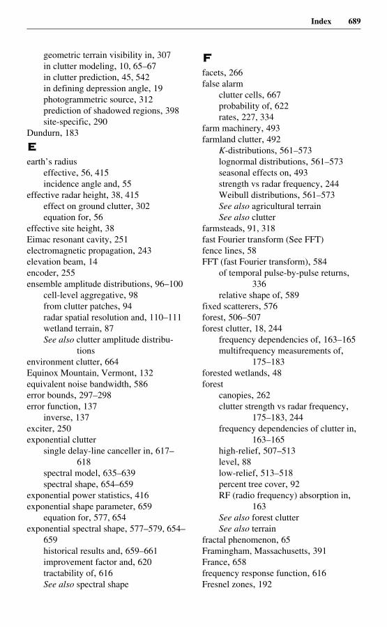
Index 689

geometric terrain visibility in, 307in clutter modeling, 10, 65–67in clutter prediction, 45, 542in defining depression angle, 19photogrammetric source, 312prediction of shadowed regions, 398site-specific, 290

Dundurn, 183

Eearth’s radius

effective, 56, 415incidence angle and, 55

effective radar height, 38, 415effect on ground clutter, 302equation for, 56

effective site height, 38Eimac resonant cavity, 251electromagnetic propagation, 243elevation beam, 14encoder, 255ensemble amplitude distributions, 96–100

cell-level aggregative, 98from clutter patches, 94radar spatial resolution and, 110–111wetland terrain, 87See also clutter amplitude distribu-

tionsenvironment clutter, 664Equinox Mountain, Vermont, 132equivalent noise bandwidth, 586error bounds, 297–298error function, 137

inverse, 137exciter, 250exponential clutter

single delay-line canceller in, 617–618

spectral model, 635–639spectral shape, 654–659

exponential power statistics, 416exponential shape parameter, 659

equation for, 577, 654exponential spectral shape, 577–579, 654–

659historical results and, 659–661improvement factor and, 620tractability of, 616See also spectral shape

Ffacets, 266false alarm

clutter cells, 667probability of, 622rates, 227, 334

farm machinery, 493farmland clutter, 492

K-distributions, 561–573lognormal distributions, 561–573seasonal effects on, 493strength vs radar frequency, 244Weibull distributions, 561–573See also agricultural terrainSee also clutter

farmsteads, 91, 318fast Fourier transform (See FFT)fence lines, 58FFT (fast Fourier transform), 584

of temporal pulse-by-pulse returns, 336

relative shape of, 589fixed scatterers, 576forest, 506–507forest clutter, 18, 244

frequency dependencies of, 163–165multifrequency measurements of,

175–183forested wetlands, 48forest

canopies, 262clutter strength vs radar frequency,

175–183, 244frequency dependencies of clutter in,

163–165high-relief, 507–513level, 88low-relief, 513–518percent tree cover, 92RF (radio frequency) absorption in,

163See also forest clutterSee also terrain

fractal phenomenon, 65Framingham, Massachusetts, 391France, 658frequency response function, 616Fresnel zones, 192

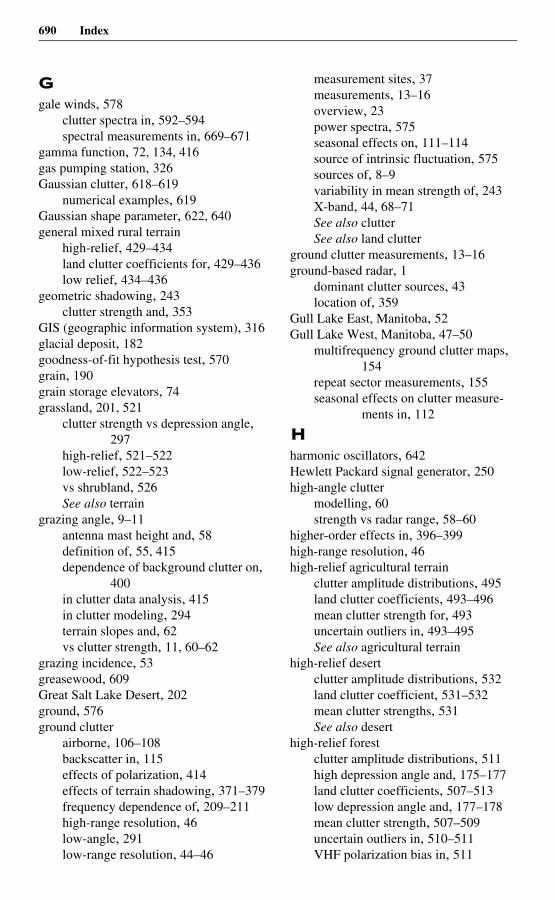
690 Index

Ggale winds, 578

clutter spectra in, 592–594spectral measurements in, 669–671

gamma function, 72, 134, 416gas pumping station, 326Gaussian clutter, 618–619

numerical examples, 619Gaussian shape parameter, 622, 640general mixed rural terrain

high-relief, 429–434land clutter coefficients for, 429–436low relief, 434–436

geometric shadowing, 243clutter strength and, 353

GIS (geographic information system), 316glacial deposit, 182goodness-of-fit hypothesis test, 570grain, 190grain storage elevators, 74grassland, 201, 521

clutter strength vs depression angle, 297

high-relief, 521–522low-relief, 522–523vs shrubland, 526See also terrain

grazing angle, 9–11antenna mast height and, 58definition of, 55, 415dependence of background clutter on,

400in clutter data analysis, 415in clutter modeling, 294terrain slopes and, 62vs clutter strength, 11, 60–62

grazing incidence, 53greasewood, 609Great Salt Lake Desert, 202ground, 576ground clutter

airborne, 106–108backscatter in, 115effects of polarization, 414effects of terrain shadowing, 371–379frequency dependence of, 209–211high-range resolution, 46low-angle, 291low-range resolution, 44–46

measurement sites, 37measurements, 13–16overview, 23power spectra, 575seasonal effects on, 111–114source of intrinsic fluctuation, 575sources of, 8–9variability in mean strength of, 243X-band, 44, 68–71See also clutterSee also land clutter

ground clutter measurements, 13–16ground-based radar, 1

dominant clutter sources, 43location of, 359

Gull Lake East, Manitoba, 52Gull Lake West, Manitoba, 47–50

multifrequency ground clutter maps, 154

repeat sector measurements, 155seasonal effects on clutter measure-

ments in, 112

Hharmonic oscillators, 642Hewlett Packard signal generator, 250high-angle clutter

modelling, 60strength vs radar range, 58–60

higher-order effects in, 396–399high-range resolution, 46high-relief agricultural terrain

clutter amplitude distributions, 495land clutter coefficients, 493–496mean clutter strength for, 493uncertain outliers in, 493–495See also agricultural terrain

high-relief desertclutter amplitude distributions, 532land clutter coefficient, 531–532mean clutter strengths, 531See also desert

high-relief forestclutter amplitude distributions, 511high depression angle and, 175–177land clutter coefficients, 507–513low depression angle and, 177–178mean clutter strength, 507–509uncertain outliers in, 510–511VHF polarization bias in, 511

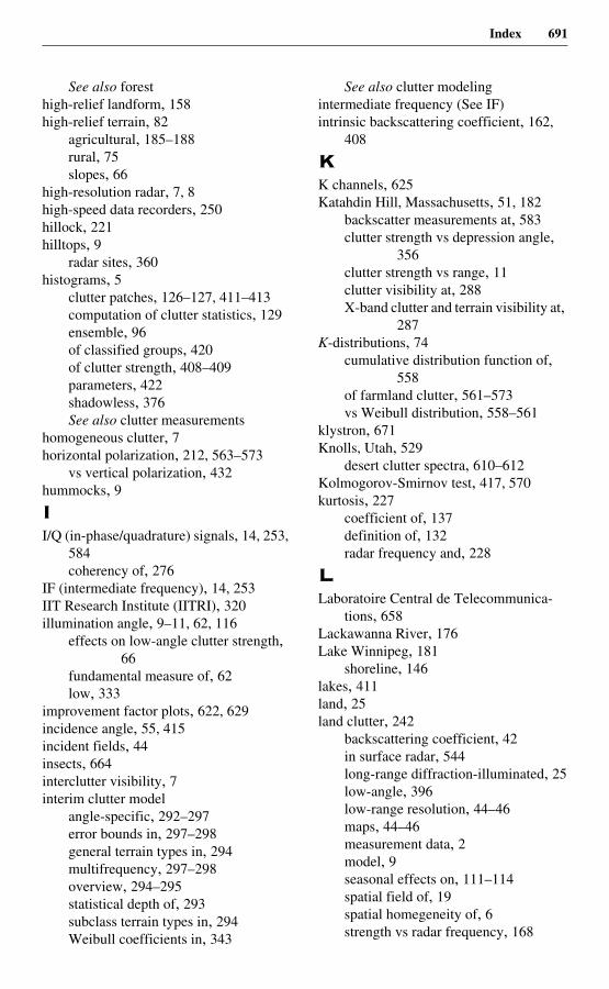
Index 691

See also foresthigh-relief landform, 158high-relief terrain, 82

agricultural, 185–188rural, 75slopes, 66

high-resolution radar, 7, 8high-speed data recorders, 250hillock, 221hilltops, 9

radar sites, 360histograms, 5

clutter patches, 126–127, 411–413computation of clutter statistics, 129ensemble, 96of classified groups, 420of clutter strength, 408–409parameters, 422shadowless, 376See also clutter measurements

homogeneous clutter, 7horizontal polarization, 212, 563–573

vs vertical polarization, 432hummocks, 9

II/Q (in-phase/quadrature) signals, 14, 253,

584coherency of, 276

IF (intermediate frequency), 14, 253IIT Research Institute (IITRI), 320illumination angle, 9–11, 62, 116

effects on low-angle clutter strength, 66

fundamental measure of, 62low, 333

improvement factor plots, 622, 629incidence angle, 55, 415incident fields, 44insects, 664interclutter visibility, 7interim clutter model

angle-specific, 292–297error bounds in, 297–298general terrain types in, 294multifrequency, 297–298overview, 294–295statistical depth of, 293subclass terrain types in, 294Weibull coefficients in, 343

See also clutter modelingintermediate frequency (See IF)intrinsic backscattering coefficient, 162,

408

KK channels, 625Katahdin Hill, Massachusetts, 51, 182

backscatter measurements at, 583clutter strength vs depression angle,

356clutter strength vs range, 11clutter visibility at, 288X-band clutter and terrain visibility at,

287K-distributions, 74

cumulative distribution function of, 558

of farmland clutter, 561–573vs Weibull distribution, 558–561

klystron, 671Knolls, Utah, 529

desert clutter spectra, 610–612Kolmogorov-Smirnov test, 417, 570kurtosis, 227

coefficient of, 137definition of, 132radar frequency and, 228

LLaboratoire Central de Telecommunica-

tions, 658Lackawanna River, 176Lake Winnipeg, 181

shoreline, 146lakes, 411land, 25land clutter, 242

backscattering coefficient, 42in surface radar, 544long-range diffraction-illuminated, 25low-angle, 396low-range resolution, 44–46maps, 44–46measurement data, 2model, 9seasonal effects on, 111–114spatial field of, 19spatial homegeneity of, 6strength vs radar frequency, 168

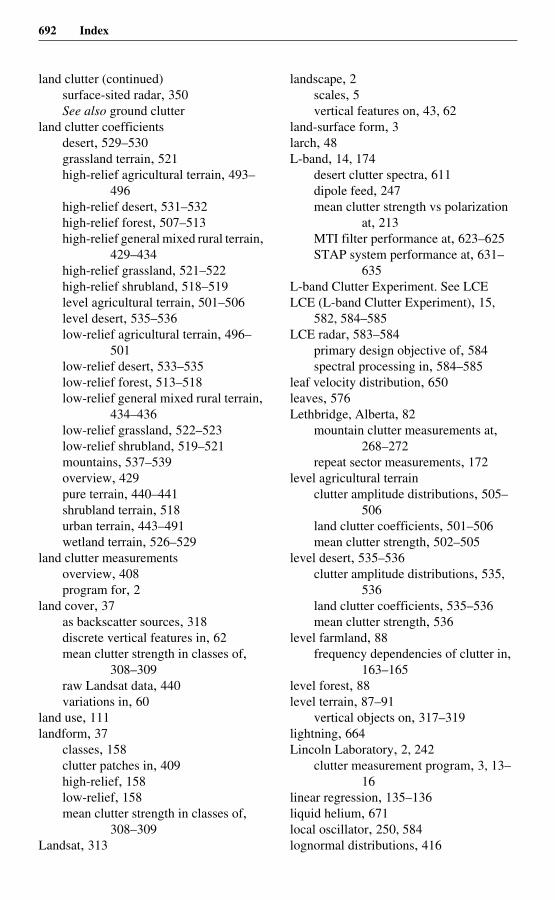
692 Index

land clutter (continued)surface-sited radar, 350See also ground clutter

land clutter coefficientsdesert, 529–530grassland terrain, 521high-relief agricultural terrain, 493–

496high-relief desert, 531–532high-relief forest, 507–513high-relief general mixed rural terrain,

429–434high-relief grassland, 521–522high-relief shrubland, 518–519level agricultural terrain, 501–506level desert, 535–536low-relief agricultural terrain, 496–

501low-relief desert, 533–535low-relief forest, 513–518low-relief general mixed rural terrain,

434–436low-relief grassland, 522–523low-relief shrubland, 519–521mountains, 537–539overview, 429pure terrain, 440–441shrubland terrain, 518urban terrain, 443–491wetland terrain, 526–529

land clutter measurementsoverview, 408program for, 2

land cover, 37as backscatter sources, 318discrete vertical features in, 62mean clutter strength in classes of,

308–309raw Landsat data, 440variations in, 60

land use, 111landform, 37

classes, 158clutter patches in, 409high-relief, 158low-relief, 158mean clutter strength in classes of,

308–309Landsat, 313

landscape, 2scales, 5vertical features on, 43, 62

land-surface form, 3larch, 48L-band, 14, 174

desert clutter spectra, 611dipole feed, 247mean clutter strength vs polarization

at, 213MTI filter performance at, 623–625STAP system performance at, 631–

635L-band Clutter Experiment. See LCELCE (L-band Clutter Experiment), 15,

582, 584–585LCE radar, 583–584

primary design objective of, 584spectral processing in, 584–585

leaf velocity distribution, 650leaves, 576Lethbridge, Alberta, 82

mountain clutter measurements at, 268–272

repeat sector measurements, 172level agricultural terrain

clutter amplitude distributions, 505–506

land clutter coefficients, 501–506mean clutter strength, 502–505

level desert, 535–536clutter amplitude distributions, 535,

536land clutter coefficients, 535–536mean clutter strength, 536

level farmland, 88frequency dependencies of clutter in,

163–165level forest, 88level terrain, 87–91

vertical objects on, 317–319lightning, 664Lincoln Laboratory, 2, 242

clutter measurement program, 3, 13–16

linear regression, 135–136liquid helium, 671local oscillator, 250, 584lognormal distributions, 416

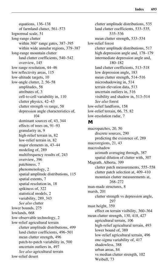
Index 693

equations, 136–138of farmland clutter, 561–573

lognormal scale, 51long-range clutter

within 360° range gates, 387–395within wide annular regions, 379–387

long-range mountain clutterland clutter coefficients, 540–542overview, 145

low range resolution, 44–46low reflectivity areas, 115low-altitude targets, 10low-angle clutter, 2, 56–58

amplitudes, 58attributes of, 3cell-to-cell variability in, 110clutter physics, 42–43clutter strength vs range, 58depression angle characteristics of,

104dominant sources of, 43, 344effects of trees on, 91–93granularity in, 9high-relief terrain in, 82low-relief terrain in, 82major elements in, 43–44modeling of, 289multifrequency results of, 243overview, 396patchiness, 7phenomenology, 2spatial amplitude distributions, 115spatial extents, 7spatial resolution in, 18spikiness of, 322statistical models, 2variability, 289, 343See also clutter

lower bounds, 275lowlands, 668low-observable technology, 2low-relief agricultural terrain

clutter amplitude distributions, 499land clutter coefficients, 496–501mean clutter strength, 496patch-to-patch variability in, 500uncertain outliers in, 497See also agricultural terrain

low-relief desert

clutter amplitude distributions, 535land clutter coefficients, 533–535,

535–536mean clutter strength, 533–534

low-relief forestclutter amplitude distributions, 517high depression angle and, 178–179intermediate depression angle and,

180–182land clutter coefficients, 513–518low depression angle, 183mean clutter strength, 514–516microshadowing in, 514terrain elevation data, 513uncertain outliers in, 516visibility and shadow in, 513–514See also forest

low-relief landform, 158low-relief terrain, 66, 75, 82low-resolution radar, 7

Mmacropatches, 20, 50

discrete sources, 290predicting the existence of, 289

macroregions, 21, 43macroshadow

azimuth averaging through, 387spatial dilution of clutter with, 307

Magrath, Alberta, 399clutter patch measurements, 555–558clutter patch selection at, 409–410mountain clutter measurements at,

268–272man-made structures, 8marsh, 201

clutter strength vs depression angle, 297

mast height, 359effect on terrain visibility, 360–364

mean clutter strength, 130, 418, 427agricultural terrain, 106high-relief agricultural terrain, 493lower bound of, 389low-relief agricultural terrain, 496one-sigma variability of, 417shadowless, 388urban areas, 84vs median clutter strength, 102Weibull, 73

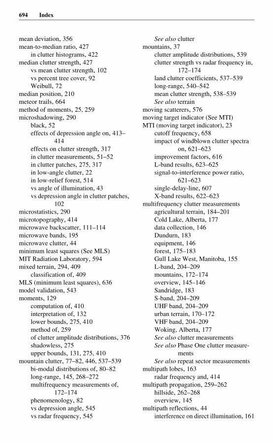
694 Index

mean deviation, 356mean-to-median ratio, 427

in clutter histograms, 422median clutter strength, 427

vs mean clutter strength, 102vs percent tree cover, 92Weibull, 72

median position, 210meteor trails, 664method of moments, 25, 259microshadowing, 290

black, 52effects of depression angle on, 413–

414effects on clutter strength, 317in clutter measurements, 51–52in clutter patches, 275, 317in low-angle clutter, 22in low-relief forest, 514vs angle of illumination, 43vs depression angle in clutter patches,

102microstatistics, 290microtopography, 414microwave backscatter, 111–114microwave bands, 195microwave clutter, 44minimum least squares (See MLS)MIT Radiation Laboratory, 594mixed terrain, 294, 409

classification of, 409MLS (minimum least squares), 636model validation, 543moments, 129

computation of, 410interpretation of, 132lower bounds, 275, 410method of, 259of clutter amplitude distributions, 376shadowless, 275upper bounds, 131, 275, 410

mountain clutter, 77–82, 446, 537–539bi-modal distributions of, 80–82long-range, 145, 268–272multifrequency measurements of,

172–174phenomenology, 82vs depression angle, 545vs radar frequency, 545

See also cluttermountains, 37

clutter amplitude distributions, 539clutter strength vs radar frequency in,

172–174land clutter coefficients, 537–539long-range, 540–542mean clutter strength, 538–539See also terrain

moving scatterers, 576moving target indicator (See MTI)MTI (moving target indicator), 23

cutoff frequency, 658impact of windblown clutter spectra

on, 621–623improvement factors, 616L-band results, 623–625signal-to-interference power ratio,

621–623single-delay-line, 607X-band results, 622–623

multifrequency clutter measurementsagricultural terrain, 184–201Cold Lake, Alberta, 177data collection, 146Dundurn, 183equipment, 146forest, 175–183Gull Lake West, Manitoba, 155L-band, 204–209mountains, 172–174overview, 145–146Sandridge, 183S-band, 204–209UHF band, 204–209urban terrain, 170–172VHF band, 204–209Woking, Alberta, 177See also clutter measurementsSee also Phase One clutter measure-

mentsSee also repeat sector measurements

multipath lobes, 163radar frequency and, 414

multipath propagation, 259–262hillside, 262–268overview, 145

multipath reflections, 44interference on direct illumination, 161

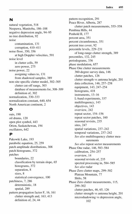
Index 695

Nnatural vegetation, 518Neepawa, Manitoba, 186–188negative depression angle, 94–95no tree distribution, 92noise

contamination, 131corruption, 410–411

noise floor, 350, 356at high Doppler velocities, 591

noise levelin clutter cells, 59zero power, 275

noise power, 22assigning values to, 131from shadowed samples, 389

non-site-specific clutter model, 302–305clutter cut-off range, 303database of measurements for, 308–309definition of, 302

normalization, 330–333normalization constant, 640, 654North American continent, 2

Ooats, 190oil drums, 120open plot symbol, 443Orion, Saskatchewan, 194oscillators, 642

PPakowki Lake, 193parabolic equation, 25, 259patch amplitude distributions, 308patch histograms, 372patches

boundaries, 22classification by terrain slope, 65histograms, 372separation, 8sizes, 8statistical convergence, 100

patchiness, 7, 286deterministic, 18spatial, 289

pattern propagation factor F, 16, 161clutter strength and, 163, 413definition of, 24, 44

pattern recognition, 291Peace River, Alberta, 287

clutter patch measurements, 555–558Pembina Hills, 44Penhold II, 177percent area, 351percent circumference, 351percent tree cover, 92percentile levels, 229–231

of long-range clutter strength, 389percentiles, 132, 245periodograms, 336phase modulation, 657Phase One clutter measurements

360-degree survey data, 146clutter patches, 126clutter strength vs antenna height, 201data collection, 146, 257–258equipment, 143, 247–254histograms, 418instruments, 13–16L-band experiments, 337multifrequency, 143objectives, 143overview, 242repeat sector, 154–156repeat sector patches, 160seasonal revisits, 235sites, 247spatial variations, 237–242temporal variations, 237–242See also multifrequency clutter mea-

surementsSee also repeat sector measurements

Phase One radar, 146, 583–584calibration, 254–257overview, 14seasonal revisits of, 235spectral processing in, 584–585See also radar

Phase Zero clutter maps, 299–302Plateau Mountain, 77Shilo, 58

Phase Zero clutter measurements, 115, 299–302clutter patches, 46, 65, 126clutter strength vs antenna height, 201microshadowing vs depression angle,

102

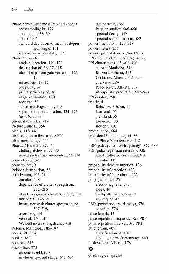
696 Index

Phase Zero clutter measurements (cont.)oversampling in, 127site heights, 38–39sites of, 37standard deviation-to-mean vs depres-

sion angle, 101summer vs winter data, 112

Phase Zero radarangle calibration, 119–120description of, 36–37, 118elevation pattern gain variation, 123–

125instrument, 13–15overview, 14primary display of, 36range calibration, 120receiver, 58schematic diagram of, 118signal strength calibration, 121–123See also radar

physical discretes, 414Picture Butte II, 356pixels, 118, 441plan position indicator. See PPIplant morphology, 111Plateau Mountain, 37, 45

clutter patches at, 77–80repeat sector measurements, 172–174

point objects, 322point source, 9Poisson distribution, 53polarization, 162, 244

circular, 598dependence of clutter strength on,

212–215effects on ground clutter strength, 414horizontal, 146, 212invariance with clutter spectra shape,

597–598overview, 144vertical, 146, 214Weibull mean strength and, 418

Polonia, Manitoba, 186–187ponds, 91, 326poplar, 182potatoes, 615power law, 575

exponent, 643, 657in clutter spectral shape, 643–654

rate of decay, 661Russian studies, 646–650spectral decay, 649spectral shape function, 582

power line pylons, 120, 318power meters, 255power spectral density (See PSD)PPI (plan position indicator), 4, 36PPI clutter maps, 13, 408–409

Altona, Manitoba, 318Brazeau, Alberta, 542Cochrane, Alberta, 324–325overview, 286Peace River, Alberta, 287site-specific prediction, 542–543

PPI display, 350prairie, 4

Beiseker, Alberta, 11farmland, 56grassland, 58low-relief, 83sloughs, 326

precipitation, 664precision IF attenuator, 14, 36

in Phase Zero receiver, 118PRF (pulse repetition frequency), 327, 583PRI (pulse repetition interval), 336

input clutter power within, 616of radar, 119

probability density function, 136probability of detection, 622probability of false alarm, 622propagation, 24–25

electromagnetic, 243lobes, 44multipath, 145, 259–262velocity of, 42

PSD (power spectral density), 576equation, 576

pulse length, 42pulse repetition frequency. See PRFpulse repetition interval. See PRIpure terrain, 409

classification of, 409land clutter coefficients for, 440

Puskwaskau, Alberta, 178

Qquadrangle maps, 64

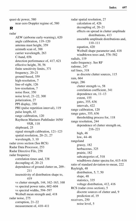
Index 697

quasi-dc power, 580near-zero Doppler regime of, 580

Rradar

AEW (airborne early-warning), 620angle calibration, 119–120antenna mast height, 359azimuth scan of, 388carrier wavelength, 263C-band, 656detection performance of, 417, 621effective height, 38, 56finite sensitivity limits, 371frequency, 20–21ground-based, 359high-resolution, 7line-of-sight, 126low-resolution, 7noise floor, 350noise level, 21–22, 300polarization, 27PPI display, 350PRI (pulse repetition interval), 119pulse length, 43range calibration, 120Raytheon Mariners Pathfinder 1650/

9XR, 118shipboard, 25signal strength calibration, 121–123spatial resolution, 20–21, 27wavelength, 3, 10

radar cross section (See RCS)Radar Data Processor, 253Radar Directive File, 258radar frequency

correlation times and, 338decoupling of, 20–21dependence of ground clutter on, 209–

211insensitivity of distribution shape to,

419vs clutter strength, 144, 162–163, 168vs spectral power ratio, 602–604vs spectral widths, 594–597Weibull mean strength and, 418

radar noise, 275corruption, 21–22measurement of, 410–411

radar spatial resolution, 27calculation of, 426decoupling of, 20–21effects on spread in clutter amplitude

distributions, 413ensemble amplitude distributions and,

110–111equation, 420Weibull shape parameter and, 418windblown trees and, 576–582

radials, 119radio frequency. See RFradome, 247rail lines, 318

as discrete clutter sources, 115rain, 664range, 286

clutter strength vs, 58correlation coefficient, 341dependence on, 11–13extent, 155gates, 355, 636intervals, 422

range calibration, 120range gates, 355, 636

thresholding process for, 118range resolution, 244

dependence of clutter strength on, 216–221

high, 46low, 44–46

rangelandgrassy, 182herbaceous, 325prairie, 182subcategories of, 518windblown clutter spectra for, 615–616

ratio of standard deviation-to-mean, 222Rayleigh, 48

distribution, 5, 7, 50slope, 48statistics, 335voltage distribution, 412, 416

RCS (radar cross section), 5discrete sources of clutter and, 9prediction of, 19

receivers, 250noise level, 5

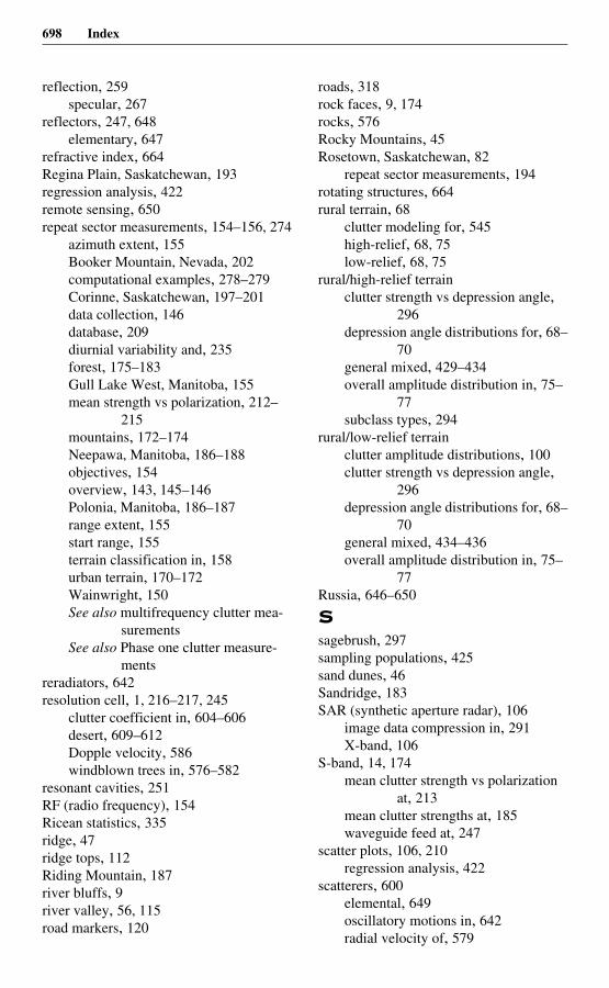
698 Index

reflection, 259specular, 267

reflectors, 247, 648elementary, 647

refractive index, 664Regina Plain, Saskatchewan, 193regression analysis, 422remote sensing, 650repeat sector measurements, 154–156, 274

azimuth extent, 155Booker Mountain, Nevada, 202computational examples, 278–279Corinne, Saskatchewan, 197–201data collection, 146database, 209diurnial variability and, 235forest, 175–183Gull Lake West, Manitoba, 155mean strength vs polarization, 212–

215mountains, 172–174Neepawa, Manitoba, 186–188objectives, 154overview, 143, 145–146Polonia, Manitoba, 186–187range extent, 155start range, 155terrain classification in, 158urban terrain, 170–172Wainwright, 150See also multifrequency clutter mea-

surementsSee also Phase one clutter measure-

mentsreradiators, 642resolution cell, 1, 216–217, 245

clutter coefficient in, 604–606desert, 609–612Dopple velocity, 586windblown trees in, 576–582

resonant cavities, 251RF (radio frequency), 154Ricean statistics, 335ridge, 47ridge tops, 112Riding Mountain, 187river bluffs, 9river valley, 56, 115road markers, 120

roads, 318rock faces, 9, 174rocks, 576Rocky Mountains, 45Rosetown, Saskatchewan, 82

repeat sector measurements, 194rotating structures, 664rural terrain, 68

clutter modeling for, 545high-relief, 68, 75low-relief, 68, 75

rural/high-relief terrainclutter strength vs depression angle,

296depression angle distributions for, 68–

70general mixed, 429–434overall amplitude distribution in, 75–

77subclass types, 294

rural/low-relief terrainclutter amplitude distributions, 100clutter strength vs depression angle,

296depression angle distributions for, 68–

70general mixed, 434–436overall amplitude distribution in, 75–

77Russia, 646–650

Ssagebrush, 297sampling populations, 425sand dunes, 46Sandridge, 183SAR (synthetic aperture radar), 106

image data compression in, 291X-band, 106

S-band, 14, 174mean clutter strength vs polarization

at, 213mean clutter strengths at, 185waveguide feed at, 247

scatter plots, 106, 210regression analysis, 422

scatterers, 600elemental, 649oscillatory motions in, 642radial velocity of, 579

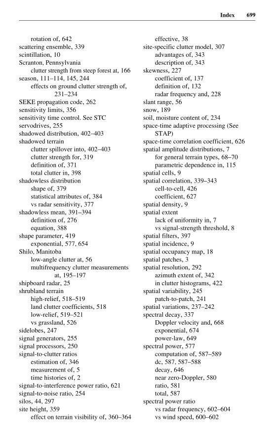
Index 699

rotation of, 642scattering ensemble, 339scintillation, 10Scranton, Pennsylvania

clutter strength from steep forest at, 166season, 111–114, 145, 244

effects on ground clutter strength of, 231–234

SEKE propagation code, 262sensitivity limits, 356sensitivity time control. See STCservodrives, 255shadowed distribution, 402–403shadowed terrain

clutter spillover into, 402–403clutter strength for, 319definition of, 371total clutter in, 398

shadowless distributionshape of, 379statistical attributes of, 384vs radar sensitivity, 377

shadowless mean, 391–394definition of, 276equation, 388

shape parameter, 419exponential, 577, 654

Shilo, Manitobalow-angle clutter at, 56multifrequency clutter measurements

at, 195–197shipboard radar, 25shrubland terrain

high-relief, 518–519land clutter coefficients, 518low-relief, 519–521vs grassland, 526

sidelobes, 247signal generators, 255signal processors, 250signal-to-clutter ratios

estimation of, 346measurement of, 5time histories of, 2

signal-to-interference power ratio, 621signal-to-noise ratio, 254silos, 44, 297site height, 359

effect on terrain visibility of, 360–364

effective, 38site-specific clutter model, 307

advantages of, 343description of, 343

skewness, 227coefficient of, 137definition of, 132radar frequency and, 228

slant range, 56snow, 189soil, moisture content of, 234space-time adaptive processing (See

STAP)space-time correlation coefficient, 626spatial amplitude distributions, 7

for general terrain types, 68–70parametric dependence in, 115

spatial cells, 9spatial correlation, 339–343

cell-to-cell, 426coefficient, 627

spatial density, 9spatial extent

lack of uniformity in, 7vs signal-strength threshold, 8

spatial filters, 397spatial incidence, 9spatial occupancy map, 18spatial patches, 3spatial resolution, 292

azimuth extent of, 342in clutter histograms, 422

spatial variability, 245patch-to-patch, 241

spatial variations, 237–242spectral decay, 337

Doppler velocity and, 668exponential, 674power-law, 649

spectral power, 577computation of, 587–589dc, 587, 587–588decay, 646near zero-Doppler, 580ratio, 581total, 587

spectral power ratiovs radar frequency, 602–604vs wind speed, 600–602

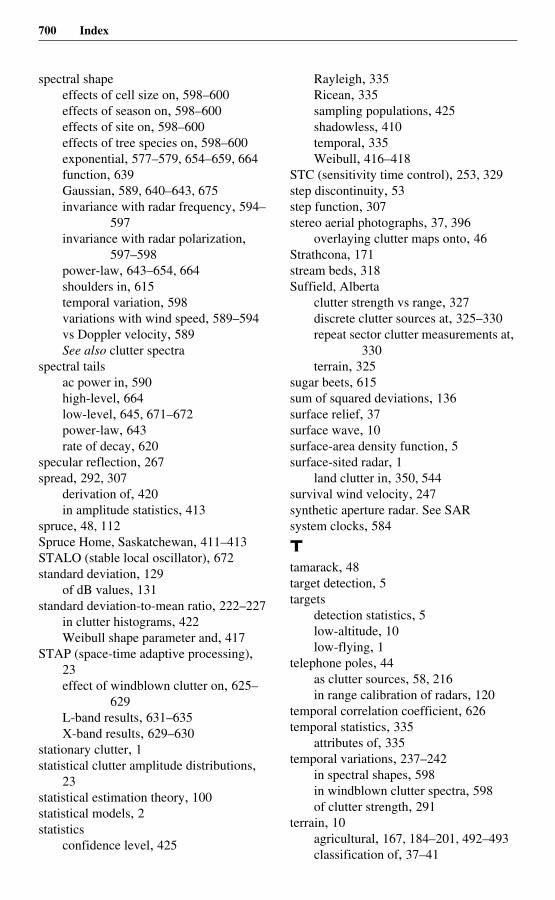
700 Index

spectral shapeeffects of cell size on, 598–600effects of season on, 598–600effects of site on, 598–600effects of tree species on, 598–600exponential, 577–579, 654–659, 664function, 639Gaussian, 589, 640–643, 675invariance with radar frequency, 594–

597invariance with radar polarization,

597–598power-law, 643–654, 664shoulders in, 615temporal variation, 598variations with wind speed, 589–594vs Doppler velocity, 589See also clutter spectra

spectral tailsac power in, 590high-level, 664low-level, 645, 671–672power-law, 643rate of decay, 620

specular reflection, 267spread, 292, 307

derivation of, 420in amplitude statistics, 413

spruce, 48, 112Spruce Home, Saskatchewan, 411–413STALO (stable local oscillator), 672standard deviation, 129

of dB values, 131standard deviation-to-mean ratio, 222–227

in clutter histograms, 422Weibull shape parameter and, 417

STAP (space-time adaptive processing), 23effect of windblown clutter on, 625–

629L-band results, 631–635X-band results, 629–630

stationary clutter, 1statistical clutter amplitude distributions,

23statistical estimation theory, 100statistical models, 2statistics

confidence level, 425

Rayleigh, 335Ricean, 335sampling populations, 425shadowless, 410temporal, 335Weibull, 416–418

STC (sensitivity time control), 253, 329step discontinuity, 53step function, 307stereo aerial photographs, 37, 396

overlaying clutter maps onto, 46Strathcona, 171stream beds, 318Suffield, Alberta

clutter strength vs range, 327discrete clutter sources at, 325–330repeat sector clutter measurements at,

330terrain, 325

sugar beets, 615sum of squared deviations, 136surface relief, 37surface wave, 10surface-area density function, 5surface-sited radar, 1

land clutter in, 350, 544survival wind velocity, 247synthetic aperture radar. See SARsystem clocks, 584

Ttamarack, 48target detection, 5targets

detection statistics, 5low-altitude, 10low-flying, 1

telephone poles, 44as clutter sources, 58, 216in range calibration of radars, 120

temporal correlation coefficient, 626temporal statistics, 335

attributes of, 335temporal variations, 237–242

in spectral shapes, 598in windblown clutter spectra, 598of clutter strength, 291

terrain, 10agricultural, 167, 184–201, 492–493classification of, 37–41

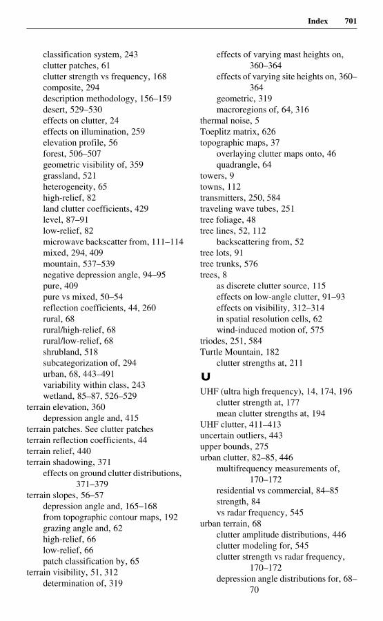
Index 701

classification system, 243clutter patches, 61clutter strength vs frequency, 168composite, 294description methodology, 156–159desert, 529–530effects on clutter, 24effects on illumination, 259elevation profile, 56forest, 506–507geometric visibility of, 359grassland, 521heterogeneity, 65high-relief, 82land clutter coefficients, 429level, 87–91low-relief, 82microwave backscatter from, 111–114mixed, 294, 409mountain, 537–539negative depression angle, 94–95pure, 409pure vs mixed, 50–54reflection coefficients, 44, 260rural, 68rural/high-relief, 68rural/low-relief, 68shrubland, 518subcategorization of, 294urban, 68, 443–491variability within class, 243wetland, 85–87, 526–529

terrain elevation, 360depression angle and, 415

terrain patches. See clutter patchesterrain reflection coefficients, 44terrain relief, 440terrain shadowing, 371

effects on ground clutter distributions, 371–379

terrain slopes, 56–57depression angle and, 165–168from topographic contour maps, 192grazing angle and, 62high-relief, 66low-relief, 66patch classification by, 65

terrain visibility, 51, 312determination of, 319

effects of varying mast heights on, 360–364

effects of varying site heights on, 360–364

geometric, 319macroregions of, 64, 316

thermal noise, 5Toeplitz matrix, 626topographic maps, 37

overlaying clutter maps onto, 46quadrangle, 64

towers, 9towns, 112transmitters, 250, 584traveling wave tubes, 251tree foliage, 48tree lines, 52, 112

backscattering from, 52tree lots, 91tree trunks, 576trees, 8

as discrete clutter source, 115effects on low-angle clutter, 91–93effects on visibility, 312–314in spatial resolution cells, 62wind-induced motion of, 575

triodes, 251, 584Turtle Mountain, 182

clutter strengths at, 211

UUHF (ultra high frequency), 14, 174, 196

clutter strength at, 177mean clutter strengths at, 194

UHF clutter, 411–413uncertain outliers, 443upper bounds, 275urban clutter, 82–85, 446

multifrequency measurements of, 170–172

residential vs commercial, 84–85strength, 84vs radar frequency, 545

urban terrain, 68clutter amplitude distributions, 446clutter modeling for, 545clutter strength vs radar frequency,

170–172depression angle distributions for, 68–

70

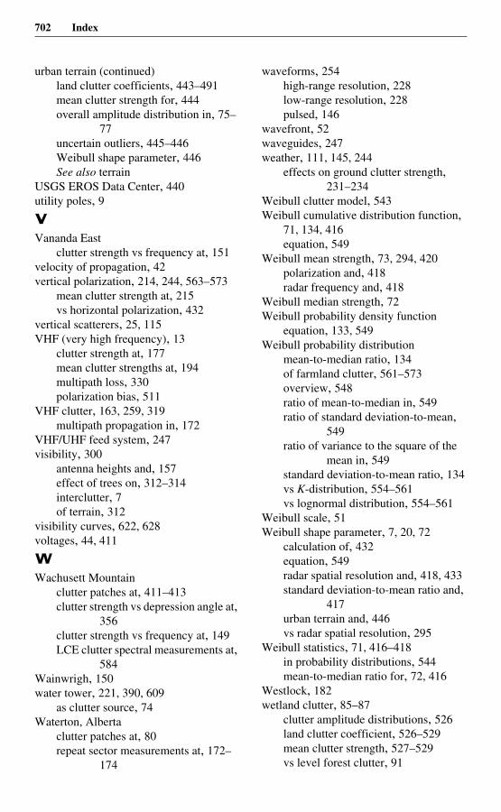
702 Index

urban terrain (continued)land clutter coefficients, 443–491mean clutter strength for, 444overall amplitude distribution in, 75–

77uncertain outliers, 445–446Weibull shape parameter, 446See also terrain

USGS EROS Data Center, 440utility poles, 9

VVananda East

clutter strength vs frequency at, 151velocity of propagation, 42vertical polarization, 214, 244, 563–573

mean clutter strength at, 215vs horizontal polarization, 432

vertical scatterers, 25, 115VHF (very high frequency), 13

clutter strength at, 177mean clutter strengths at, 194multipath loss, 330polarization bias, 511

VHF clutter, 163, 259, 319multipath propagation in, 172

VHF/UHF feed system, 247visibility, 300

antenna heights and, 157effect of trees on, 312–314interclutter, 7of terrain, 312

visibility curves, 622, 628voltages, 44, 411

WWachusett Mountain

clutter patches at, 411–413clutter strength vs depression angle at,

356clutter strength vs frequency at, 149LCE clutter spectral measurements at,

584Wainwrigh, 150water tower, 221, 390, 609

as clutter source, 74Waterton, Alberta

clutter patches at, 80repeat sector measurements at, 172–

174

waveforms, 254high-range resolution, 228low-range resolution, 228pulsed, 146

wavefront, 52waveguides, 247weather, 111, 145, 244

effects on ground clutter strength, 231–234

Weibull clutter model, 543Weibull cumulative distribution function,

71, 134, 416equation, 549

Weibull mean strength, 73, 294, 420polarization and, 418radar frequency and, 418

Weibull median strength, 72Weibull probability density function

equation, 133, 549Weibull probability distribution

mean-to-median ratio, 134of farmland clutter, 561–573overview, 548ratio of mean-to-median in, 549ratio of standard deviation-to-mean,

549ratio of variance to the square of the

mean in, 549standard deviation-to-mean ratio, 134vs K-distribution, 554–561vs lognormal distribution, 554–561

Weibull scale, 51Weibull shape parameter, 7, 20, 72

calculation of, 432equation, 549radar spatial resolution and, 418, 433standard deviation-to-mean ratio and,

417urban terrain and, 446vs radar spatial resolution, 295

Weibull statistics, 71, 416–418in probability distributions, 544mean-to-median ratio for, 72, 416

Westlock, 182wetland clutter, 85–87

clutter amplitude distributions, 526land clutter coefficient, 526–529mean clutter strength, 527–529vs level forest clutter, 91

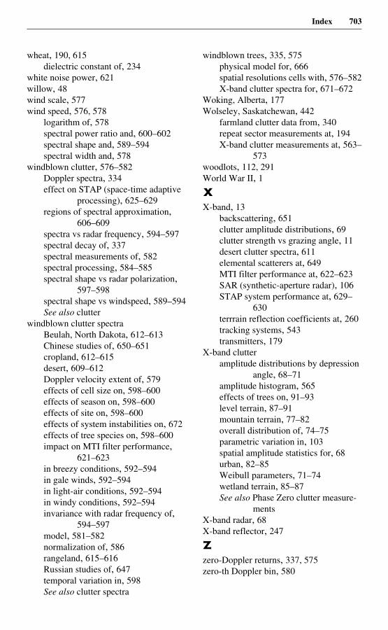
Index 703

wheat, 190, 615dielectric constant of, 234

white noise power, 621willow, 48wind scale, 577wind speed, 576, 578

logarithm of, 578spectral power ratio and, 600–602spectral shape and, 589–594spectral width and, 578

windblown clutter, 576–582Doppler spectra, 334effect on STAP (space-time adaptive

processing), 625–629regions of spectral approximation,

606–609spectra vs radar frequency, 594–597spectral decay of, 337spectral measurements of, 582spectral processing, 584–585spectral shape vs radar polarization,

597–598spectral shape vs windspeed, 589–594See also clutter

windblown clutter spectraBeulah, North Dakota, 612–613Chinese studies of, 650–651cropland, 612–615desert, 609–612Doppler velocity extent of, 579effects of cell size on, 598–600effects of season on, 598–600effects of site on, 598–600effects of system instabilities on, 672effects of tree species on, 598–600impact on MTI filter performance,

621–623in breezy conditions, 592–594in gale winds, 592–594in light-air conditions, 592–594in windy conditions, 592–594invariance with radar frequency of,

594–597model, 581–582normalization of, 586rangeland, 615–616Russian studies of, 647temporal variation in, 598See also clutter spectra

windblown trees, 335, 575physical model for, 666spatial resolutions cells with, 576–582X-band clutter spectra for, 671–672

Woking, Alberta, 177Wolseley, Saskatchewan, 442

farmland clutter data from, 340repeat sector measurements at, 194X-band clutter measurements at, 563–

573woodlots, 112, 291World War II, 1

XX-band, 13

backscattering, 651clutter amplitude distributions, 69clutter strength vs grazing angle, 11desert clutter spectra, 611elemental scatterers at, 649MTI filter performance at, 622–623SAR (synthetic-aperture radar), 106STAP system performance at, 629–

630terrrain reflection coefficients at, 260tracking systems, 543transmitters, 179

X-band clutteramplitude distributions by depression

angle, 68–71amplitude histogram, 565effects of trees on, 91–93level terrain, 87–91mountain terrain, 77–82overall distribution of, 74–75parametric variation in, 103spatial amplitude statistics for, 68urban, 82–85Weibull parameters, 71–74wetland terrain, 85–87See also Phase Zero clutter measure-

mentsX-band radar, 68X-band reflector, 247

Zzero-Doppler returns, 337, 575zero-th Doppler bin, 580