Love for Quality, Comparative Advantage, and Trade�

Esteban Jaimovichy Vincenzo Merellaz

This Version: July 2013

First Version: March 2011

Abstract

We propose a Ricardian trade model with horizontal and vertical di¤erentiation, where individ-

uals�willingness to pay for quality rises with their income, and productivity di¤erentials across

countries are stronger for high-quality goods. Our theory predicts that the scope for trade

widens and international specialisation intensi�es as incomes grow and wealthier consumers

raise the quality of their consumption baskets. This implies that comparative advantages inten-

sify gradually over the path of development as a by-product of the process of quality upgrading.

The evolution of comparative advantages leads to speci�c trade patterns that change over the

growth path, by linking richer importers to more specialised exporters. We provide empirical

support for this prediction, showing that the share of imports originating from exporters ex-

hibiting a comparative advantage in a speci�c product correlates positively with the importer�s

GDP per head.

Keywords: International Trade, Nonhomothetic Preferences, Quality Ladders.

JEL Classi�cations: F11, F43, O40

�We would like to thank Andrea Carriero, Arnaud Costinot, Pablo Fajgelbaum, Giovanni Mastrobuoni, Ignacio

Monzon, Alessio Moro, Juan Pablo Rud and Ina Simonovska for comments and suggestions, as well as seminar

participants at Bologna University, Bristol University, Collegio Carlo Alberto, University of St. Gallen, University

of Surrey, University of Cagliari, Queen Mary, the SED Meeting (Seoul), the RIEF Meeting (Bocconi), the Royal

Economic Society Meeting (Cambridge), and the Midwest International Trade Meeting (Washington University).

yUniversity of Surrey and Collegio Carlo Alberto. Mailing address: School of Economics, Guildford, GU2 7XH,

United Kingdom. Email: e.jaimovich@surrey.ac.uk

zUniversity of Cagliari. Mailing address: Department of Economics and Business, Viale Sant�Ignazio 17, 09123

Cagliari, Italy. Email: merella@unica.it.

1

1 Introduction

Income is a key determinant of consumer choice. A crucial dimension through which purchasing

power in�uences this choice is the quality of consumption. People with very di¤erent incomes

tend to consume commodities within the same category of goods, such as clothes, cars, wines, etc.

However, the actual quality of the consumed commodities di¤ers substantially when looking at

poorer versus richer households. The same reasoning naturally extends to countries with di¤erent

levels of income per capita. In this case, the quality dimension of consumption entails important

implications on the evolution of trade �ows.

Several recent studies have investigated the links between quality of consumption and interna-

tional trade. One strand of literature has centred their attention on the demand side, �nding a

strong positive correlation between quality of imports and the importer�s income per head [Hallak

(2006), Fieler (2011a)].1 On the other hand, a set of papers have focused on whether exporters

adjust the quality of their production to serve markets with di¤erent income levels. The evidence

here also points towards the presence of nonhomothetic preferences along the quality dimension,

showing that producers sell higher quality versions of their output to richer importers.2

These empirical �ndings have motivated a number of models that yield trade patterns where

richer importers buy high-quality versions of goods, while exporters di¤erentiate the quality of

their output by income at destination [Hallak (2010), Fajgelbaum, Grossman and Helpman (2011),

Jaimovich and Merella (2012)]. Yet, this literature has approached the determinants of countries�

sectoral specialisation as a phenomenon that is independent of the process of quality upgrading

resulting from higher consumer incomes. This paper investigates whether exchanging higher or

lower quality versions of output a¤ects the categories of goods that countries specialise in, and the

intensity of trade links that they establish with di¤erent importers. We propose a theory where

quality upgrading in consumption becomes the central driving force behind a general process of

comparative advantage intensi�cation and varying bilateral trade links at di¤erent levels of income.

Our theory is grounded on the hypothesis that productivity di¤erentials are stronger for higher-

1See also related evidence in Choi, Hummels and Xiang (2009), Francois and Kaplan (1996) and Dalgin, Trindade

and Mitra (2008).2For example, Verhoogen (2008) and Iacovone and Javorcik (2008) provide evidence of Mexican manufacturing

plants selling higher qualities in US than in their local markets. Brooks (2006) establishes the same results for

Colombian manufacturing plants, and Manova and Zhang (2012) show that Chinese �rms ship higher qualities of

their exports to richer importers. Analogous evidence is provided by Bastos and Silva (2010) for Portuguese �rms,

and by Crino and Epifani (2012) for Italian ones.

2

quality goods, combined with the notion that willingness to pay for quality rises with income.

Within this framework, we show that international specialisation and trade intensify over the

growth path. The evolution of trade �ows featured by our model presents novel speci�cities

that stem from the interaction between nonhomothetic preferences and the deepening of sectoral

productivity di¤erentials at higher levels of quality. In particular, the process of quality upgrading

with rising income sets in motion both demand-driven and supply-driven factors, leading to a

simultaneous rise in specialisation by importers and exporters over the growth path. Import and

export specialisation take place together precisely because, as countries become richer, consumers

shift their spending towards high-quality goods, which are exactly those that tend to display greater

scope for export specialisation.

We model a world economy with a continuum of horizontally di¤erentiated goods, each of them

available in a continuum of vertically ordered quality levels. Each country produces a particular

variety of every good. The production technology di¤ers both across countries and sectors. We

assume that some countries are intrinsically better than others in producing certain types of goods.

In addition, these intrinsic productivity di¤erentials on the horizontal dimension tend to become

increasingly pronounced along the vertical dimension. These assumptions lead to an intensifying

process of Ricardian specialisation as production moves up on the quality ladders of each good.

For example, a country may have a cost advantage in producing wine, while another country may

have it in whisky. This would naturally lead them to exchange these two goods. Yet, in our model,

productivity di¤erences in the wine and whisky industries do not remain constant along the quality

space, but become more intense as production moves up towards higher quality versions of those

goods. As a result, the scope for international trade turns out to be wider for high-quality wines

and whiskies than for low-quality ones.

We combine such a production structure with nonhomothetic preferences on the quality dimen-

sion. This implies that, given market prices, richer individuals consume higher quality versions of

the di¤erentiated goods. Within this framework, we show that at low levels of income both export

and import specialisation remain low. The reason for this result is that productivity di¤erentials

across �rms from di¤erent economies are relatively narrow for goods o¤ered in low quality versions.

However, in a growth context, as individuals upgrade their quality of consumption, sectoral pro-

ductivity di¤erentials deepen, which in turn leads to a gradual process of increasing international

specialisation.

Our model thus suggests that the study of the evolution of trade links may require considering

a more �exible concept of comparative advantage than the one traditionally used in the literature,

3

so as to encompass quality upgrading as an inherent part of it. In the literature of Ricardian

trade, the comparative advantage is solely determined by exporters� technologies. This paper

instead sustains that both the importers�incomes and the exporters�sectoral productivities must

be taken into account in order to establish a rank of comparative advantage. This is because the

degree of comparative advantage between any two countries is crucially a¤ected by the quality

of consumption of their consumers. As a consequence, richer and poorer importers may end up

establishing trade links with di¤erent partners, simply because the gaps between their willingness-

to-pay for quality may translate into unequal degrees of comparative advantage with respect to

the same set of exporters.

The conditionality of comparative advantage on importers incomes entails clear and testable

predictions on the evolution of trade �ows. In particular, the model yields predictions that link

di¤erent importers to speci�c exporters. According to our model, the share of imports originating

from exporters exhibiting a cost advantage in a given good must grow with the income per head

of the importer. This would be the result of richer importers buying high-quality versions of

goods, which are the type of commodities for which cost di¤erentials across countries are relatively

more pronounced. In that regard, we �rst test the notion that productivity di¤erentials deepen at

higher levels of quality of production. Next, we provide evidence consistent with the prediction that

richer economies are more likely to buy their imports from producers who display a comparative

advantage in the imported goods.

Related Literature

Nonhomothetic preferences are by now a widespread modelling choice in the trade literature.

However, most of the past trade literature with nonhomotheticities has focused either on vertical

di¤erentiation [e.g., Flam and Helpman (1987), Stokey (1991) and Murphy and Shleifer (1997)]

or horizontal di¤erentiation in consumption [e.g., Markusen (1986), Bergstrand (1990) and Mat-

suyama (2000)].3 Two recent articles have combined vertical and horizontal di¤erentiation with

preferences featuring income-dependent willingness to pay for quality: Fajgelbaum, Grossman and

Helpman (2011) and Jaimovich and Merella (2012).

Fajgelbaum et al. (2011) analyse how di¤erences in income distributions between economies3For some recent contributions with horizontal di¤erentiation and nonhomothetic preferences see, for example:

Foellmi, Hepenstrick and Zweimuller (2010) and Tarasov (2012), where consumers are subject to a discrete consump-

tion choice (they must consume either zero or one unit for each good), and Fieler (2011b) who, using a CES utility

function, ties the income elasticity of consumption goods across di¤erent industries to the degree of substitution of

goods within the same industry.

4

with access to the same technologies determine trade �ows in the presence of increasing returns

and trade cost. Like ours, their paper leads to an endogenous emergence of comparative advantages,

which may have remained latent for quite some time (either due to trade costs being too high or

countries� income distributions being too similar). Our paper, instead, sticks to the Ricardian

tradition where trade is the result of di¤erences in technologies featuring constant returns to scale.

In particular, in our model, comparative advantages and trade emerge gradually, not because trade

costs obstruct the course of increasing returns, but because the demand for commodities displaying

wider heterogeneity in cost of production (i.e., high-quality goods) expands as incomes rise. In that

respect, an important di¤erence between the two papers is the reason why high-quality versions of

goods are inherently more tradable than low-quality ones: in Fajgelbaum et al. (2011) this is due

to quality-speci�c trade costs, while in our model it is the result of technological factors.

Jaimovich and Merella (2012) also propose a nonhomothetic preference speci�cation where

budget reallocations take place both within and across horizontally di¤erentiated goods. That pa-

per, however, remained within a standard Ricardian framework where absolute and comparative

advantages are determined from the outset, and purely by technological conditions. Hence, nonho-

mothetic preferences play no essential role there in determining export and import specialisation

at di¤erent levels of development. By contrast, it is the interaction between rising di¤erences in

productivity at higher quality levels and nonhomotheticities in quality that generates our novel

results in terms of co-evolution of export and import specialisation.

A key assumption in our theory is the widening in productivity di¤erentials at higher levels of

quality. To the best of our knowledge, Alcala (2012) is the only other paper that has explicitly

introduced a similar feature into a Ricardian model of trade. An important di¤erence between

the two papers is that Alcala�s keeps the homothetic demand structure presented in Dornbusch,

Fisher and Samuelson (1977) essentially intact. Nonhomotheticities in demand are actually crucial

to our story and, in particular, to its main predictions regarding the evolution of trade �ows and

specialisation at di¤erent levels of income.

Finally, Fieler (2011b) also studies the interplay between nonhomothetic demand and Ricardian

technological disparities. She shows that, when productivity di¤erences are stronger for goods with

high income elasticity, her model matches quite closely key features of North-North and North-

South trade. Our model di¤ers from hers in that the e¤ects of demand on trade stem from the

allocation of spending within categories of goods rather than across them. Our results therefore

hinge on richer consumers switching their good-speci�c expenditure shares from lower-quality to

higher-quality versions of the goods. It is in fact this within-good substitution process that leads

5

to our predictions of income-dependent spending shares across di¤erent exporters.4

The rest of the paper is organised as follows. Section 2 studies a world economy with a

continuum of countries where all economies have the same level of income per head in equilibrium.

Section 3 generalises the main results to a world economy where some countries are richer than

others. Section 4 presents some empirical results consistent with the main predictions of our model.

Section 5 concludes. All relevant proofs can be found in the Appendices.

2 A world economy with equally rich countries

We study a world economy with a unit continuum of countries indexed by v 2 V. In each country

there is a continuum of individuals with unit mass. Each individual is endowed with one unit of

labour time. We assume labour is immobile across countries. In addition, we assume all countries

are open to international trade, and there are no trading costs of any sort.

Our model will display two main distinctive features: �rst, productivity di¤erentials across

countries will rise with the quality level of the commodities being produced; second, richer individ-

uals will choose to consume higher-quality commodities than poorer ones. Subections 2.2 and 2.3

specify the functional forms of production technologies and consumer preferences that we adopt to

generate these two features. In subsection 2.1 we describe formally the set of consumption goods

in our world economy.

2.1 Commodity space

All countries share a common commodity space de�ned along three distinct dimensions: a hori-

zontal, a varietal, and a vertical dimension.

Concerning the horizontal dimension, there exists a unit continuum of di¤erentiated goods,

indexed by z, where z 2 Z = [0; 1]. In terms of the varietal dimension, we assume that each country

v 2 V = [0; 1] produces a speci�c variety v of each good z. Finally, our vertical dimension refers to

the intrinsic quality of the commodity: a continuum of di¤erent qualities q, where q 2 Q = [1;1),

are potentially available for every variety v of each good z. As a result, in our setup, each

commodity is designated by a speci�c good-variety-quality index, (z; v; q) 2 Z� V�Q.

To �x ideas, the horizontal dimension refers to di¤erent types of goods, such as cars, wines,

4 In this respect, our paper relates also to Linder (1961) and Hallak (2010) views of quality as an important

dimension in explaining trade �ows between countries of similar income levels. We propose a new mechanism that

links together quality of production, income per capita and trade at di¤erent stages of development.

6

co¤ee beans, etc. The varietal dimension refers to the di¤erent varieties of any given type of good,

originating from di¤erent countries, such as Spanish and French wines (di¤ering, for instance, in

speci�c traits like the types of grapes and regional vini�cation techniques). The vertical dimension

refers to the intrinsic quality of each speci�c commodity (e.g., the ageing and the grapes selection

in the winemaking).5

2.2 Production technologies

In each country v there exists a continuum of �rms in each sector z that may transform local

labour into a variety v of good z. Production technologies are idiosyncratic both to the sector z

and to the country v. In particular, we assume that, in order to produce one unit of commodity

(z; v; q), a �rm from country v in sector z needs to use �z;v (q) units of labour, where:

�z;v (q) = e��(��1)=(��1) q

�z;v

1 + �: (1)

Unit labour requirements contain two key technological parameters. The �rst is � > 0, which

applies identically to all sectors and countries, and we interpret it as the worldwide total factor

productivity level. As such, in our model, increases in � will capture the e¤ects of aggregate growth

and rising real incomes. The second is �z;v, which may di¤er both across z and v, and governs

the elasticity of the labour requirements with respect to quality upgrading. In what follows, we

assume that each parameter �z;v is independently drawn from a probability density function with

uniform distribution over the interval��; ��. In addition, we assume that � > 1. Hence, �z;v (q)

are always strictly increasing and convex in q.

To ease notation, we will henceforth denote A � e��(��1)=(��1). Notice that the parameter A

is simply a scale factor between labour input units and quality units. We include this additional

term only to help simplifying the algebra of the consumer�s optimisation problem to be presented

in the following subsection.6

5We should stress that while the horizontal and the vertical dimensions (z and q, respectively) are crucial ingre-

dients to our story, the varietal dimension (v) is only subsidiary to it. In that respect, our commodity space could

be seen as an extension of that in Dornbusch, Fischer and Samuelson (1977) exhibiting a quality ladder within each

sector z. The main reason why we include also the varietal dimension v is to (possibly) allow more than one country

to actively produce each good at a certain quality level. More precisely, we wish to leave room for the model to

determine the degree of specialisation of each country v in good z at quality level q, rather than having only one

economy producing each good z at a speci�c level of quality.6All our main results hold qualitatively true when the labour income requirement are given by �z;v (q) = q�z;v=(1+

�), only at the cost of more tedious algebra.

7

Remark 1 (Cost advantage along the quality space) Our speci�cation of �z;v (q) charac-

terizes the �rst key feature of our model: cross-country productivity di¤erentials rise with the

level of quality of production. For any given good z, the unit labour requirement in country v00 rel-

ative to country v0 increases with quality q whenever �z;v0 < �z;v00. Formally, the derivative of the

ratio �z;v00 (q) =�z;v0 (q) = q�z;v00��z;v0 with respect to q yields

��z;v00 � �z;v0

�q�z;v00��z;v0�1, which is

positive for any q 2 Q. In our model, this will in turn imply that the cost advantage of the country

with the better sectoral productivity draw will widen up along the quality dimension of production.

Let wv denote henceforth the wage per unit of labour time in country v. Assuming that all �rms

in each sector z of country v have access to the same technology (that is, sectoral productivities

di¤er only across �rms in di¤erent countries), perfect competition within countries ensures that

all commodities will be priced exactly at their unit cost. That is:

pz;v;q = Aq�z;v

1 + �wv; for all (z; v; q) 2 Z� V�Q. (2)

From (2) it follows that changes in � leave all relative prices unaltered. In this regard, we may

consider a rise in total factor productivity as an increase in real income, as it entails no substitution

e¤ect across the di¤erent commodities.7

2.3 Preferences and budget constraint

All individuals in the world share identical preferences de�ned over the good-variety-quality space

described in Section 2.1.

To simplify the analysis, we preliminarily introduce the following assumption:

Assumption 1 (Selection of quality) For each good-variety pair (z; v) 2 Z� V, individuals

consume a strictly positive amount of physical quantity of only one quality version of it.

Assumption 1 is analogous to assuming an in�nite elasticity of substitution across di¤erent quality

versions of the good z sourced from country v.8 Henceforth, to ease notation, we denote the7One may be tempted to infer from (2) that a rise in � leads to a lower price of quality. However, this would

only be an appropriate interpretation if individuals were supposed to consume a single unit of each good, as it is

the case for example in Flam and Helpman (1987). As it will become clearer in the next subsection, in our model

individuals do not purchase quality directly, but only via physical units of commodities that embody a certain level

of quality. Moreover, since physical consumption is not restricted to one unit per good, a higher � reduces, through

(2), the cost of any combination of quantity and quality in the same proportion.8See equation (20) in Appendix A for the derivation of utility (3) replacing Assumption 1 by an in�nite elasticity

of substitution across di¤erent quality versions of z sourced from v.

8

selected quality of variety v of good z simply by qz;v. In addition, we denote by cz;v the consumed

physical quantity of the selected quality qz;v.

Preferences are de�ned over the physical quantities fcz;vg consumed in the selected quality

levels fqz;vg. We let preferences be summarised by the following utility function:

U =

�ZZ

�ZVln (cz;v)

qz;v dv

��dz

� 1�

; where � < 0: (3)

Individuals choose the physical quantity to consume for each of the selected qualities, subject

to the budget constraint: ZZ

�ZV

�A

1 + �(qz;v)

�z;v wv

�cz;v dv

�dz � w, (4)

where we have already substituted the price pz;v of each consumed commodity qz;v by its expression

as a function of technological parameters and wage according to (2).9

The utility function (3) displays a number of features that is worth discussing in further detail.

Firstly, considering the quality dimension in isolation, the exponential terms f(cz;v)qz;vg in (3) are

instrumental to obtaining our desired non-homothetic behaviour along the quality space. As the

remark below formally describes, the exponential functional form implies that, whenever cz;v > 1,

the magnifying e¤ect of quality becomes increasingly important as cz;v rises. Such non-homothetic

feature in turn leads to a solution of the consumer problem where higher real incomes �which

could be generated either by increases in � or in w in the budget constraint (4)�will translate into

quality upgrading of consumption.

Remark 2 (Nonhomotheticities along the quality dimension) The terms f(cz;v)qz;vg in (3)

lead to preferences that are nonhomothetic along the quality dimension of the commodity space.

Abstracting for a moment from Assumption 1, this can be seen by taking any two qualities levels

q < q of the same commodity (z; v) and observing that the marginal rate of substitution of the

physical quantities of consumption at those quality levels, namely cz;v;q for cz;v;q, is non-decreasing

9Rigorously speaking, our preference speci�cation should be written down as follows:

U =

�ZZ

�ZVln (max fcz;v; cz;vqz;vg) dv

��dz

� 1�

;

so that raising the quality of a given quantity of consumption is never bad for the consumer. Notice that in the max

operator the term cz;v applies whenever 0 � cz;v < 1, while cz;vqz;v applies whenever cz;v � 1. Since according to

(2) prices are strictly increasing in q, it turns out that individuals would choose qz;v > 1 only if cz;v > 1; otherwise

the simply set qz;v = 1. For this reason we can simplify the expression to (3) at no analytical cost to our results.

9

along a proportional expansion path of cz;v;q and cz;v;q.10

Secondly, abstracting now from the quality dimension, (3) features two nested CES functions.

On the one hand, for each good z, the (inner) logarithmic function bundling the exponential terms

of the varieties sourced from the di¤erent countries v 2 V implies a unit elasticity of substitution

across varieties of the same good z. On the other hand, the parameter � < 0 characterizing the

(outer) function mapping the bundles of the di¤erent goods z 2 Z into utility U implies that the

elasticity of substitution across goods is equal to 1= (1� �) < 1. The speci�cation in (3) then

intends to capture the notion that the elasticity of substitution across di¤erent goods is smaller

than within goods (i.e., across the di¤erent varieties of the same good).

2.4 Utility maximisation

When optimising (3) subject to (4) we must take into account the fact that the consumer�s income

may well di¤er across countries. Hereafter, we use the letter i 2 V to refer to the country of

origin of a speci�c consumer, and we use i as a superindex any time we refer to choices made by

consumers from country i.

The consumer�s problem requires choosing combinations of (non-negative) quantities on the

good-variety-quality commodity space, subject to (4). However, it turns out that the optimisation

problem may be simpli�ed by letting �iz;v denote the demand intensity in country i 2 V for the

variety v 2 V of good z 2 Z. Accordingly, we may note that ciz;v = �iz;vwi=pz;v (where recall that

pz;v is the market price of commodity qz;v). Hence, using (2), we may write:

ciz;v =�iz;vwi�

qiz;v��z;v wvA=(1 + �) : (5)

We may then restate the original consumer�s optimisation problem into one de�ned only in

terms of optimal seclected qualities and optimal budget allocations across varieties of goods. Below

we state the reformulated consumer�s problem.

An individual from country i 2 V chooses the optimal quality qiz;v and optimal budget allocation10Formally, this can be observed by computing MRS(cz;v;q; cz;v;q) from utility (20) in Appendix A. Then, along

a proportional expansion path cz;v;q = k cz;v;q, where k > 0, we have that:

MRS�k cz;v;q; cz;v;q

�=�q=q�kq�1

�cz;v;q

�q�q;

which is increasing for any cz;v;q > 1.

10

�iz;v for each (z; v) 2 Z� V, so as to solve:11

maxfqiz;v ;�iz;vg(z;v)2Z�V

U =

(ZZ

"ZVqiz;v ln

1 + �

A

�iz;v�qiz;v��z;v wiwv

!dv

#�dz

) 1�

subject to:ZZ

ZV�iz;v dv dz = 1; and qiz;v 2 Q, for all (z; v) 2 Z� V:

(6)

We can observe that relative wages (wi=wv) may play a role in the optimisation problem (6).

For the time being, we will shut down this channel, and characterise the solution of (6) only for

the case in which wages are the same in all countries. (Indeed, as it will be shown next, in this

speci�cation of the model all wages will turn out to be equal in equilibrium.)

Lemma 1 When wv = w for all v 2 V, problem (6) yields, for all (z0; v0) 2 Z� V:

qiz0;v0 =

"(1 + �) =A

e�z0;v0RZRV q

iz;v dv dz

#1=(�z0;v0�1); (7)

�iz0;v0 =

"(1 + �) =A�

eRZRV q

iz;v dv dz

��z0;v0#1=(�z0;v0�1)

: (8)

In addition, @qiz0;v0=@� > 0.

Proof. In Appendix A.

Lemma 1 characterises the solution of the consumer�s problem in terms of two sets of variables:

(i) the expressions in (7), which stipulate the quality level in which each variety of every horizon-

tally di¤erentiated good is optimally consumed; (ii) the expressions in (8) describing the optimal

expenditure shares allocated to those commodities. Furthermore, the result @qiz;v=@� > 0 sum-

marises the key nonhomothetic behaviour present in our model: quality upgrading of consumption.

That is, as real incomes grow with a rising �, individuals substitute (previously selected) lower-

quality versions of every variety v of each good z by (previously not consumed) better versions of

them.12

11A formal solution of problem (6) is provided in Appendix A.

12Note that variations in � a¤ect all prices in (2) in the same proportion, leaving all relative prices unchanged. In

that regard, a rise in � leads consumers to upgrade their quality of consumption via a pure income-e¤ect, without

any substitution-e¤ect across quality versions of the same variety. In fact, a rise in � entails the same e¤ects as an

exogenous increase of wi in (6).

11

2.5 Equilibrium and specialisation

In equilibrium, total world spending on commodities produced in country v must equal the total

labour income in country v (which is itself equal to the total value of goods produced in v). Bearing

in mind (6), we may then write down the market clearing conditions as follows:ZZ

ZV�iz;v wi di dz = wv, for all v 2 V: (9)

More formally, an equilibrium in the world economy is given by a set of wages fwvgv2V such

that: i) prices of all traded commodities are determined by (2); ii) consumers from country i 2 V

choose their allocations�qiz;v; �

iz;v

(z;v)2Z�V by solving (6); and iii) the market clearing conditions

stipulated in (9) hold simultaneously for all countries.

Proposition 1 Suppose that, for each commodity (z; v) 2 Z�V, �z;v is independently drawn from

a uniform density function with support��; ��. Then, for any � > 0, in equilibrium: wv = w for

all v 2 V.

Proof. In Appendix A.

Proposition 1 shows that, in this (symmetric) world economy, the equilibrium relative wages

remain unchanged and equal to unity all along the growth path. The reason for this result is the

following: as � rises, and real incomes accordingly increase, aggregate demands and supplies grow

together at identical speed in all countries. As a consequence, markets clearing conditions in (9)

will constantly hold true without the need of any adjustment in relative wages across economies.

The equiproportional aggregate variations implicit in Proposition 1 conceal the fact that, as �

increases, economies actually experience signi�cant changes in their consumption and production

structures at the sectoral level. In other words, although aggregate demands and supplies change

at the same speed in all countries, sectoral demands and supplies do not, which in turn leads to

country-speci�c processes of labour reallocation across sectors. Such sectoral reallocations of labour

stem from the interplay of demand and supply side factors. On the demand side, as real incomes

grow with a rising �, individuals start consuming higher quality varieties of each commodity �

as can be observed from (7). On the supply side, heterogeneities in sectoral labour productivities

across countries become stronger as producers raise the quality of their output. Hence, the interplay

between income-dependent willingness to pay for quality and intensi�cation of sectoral productivity

di¤erences at higher levels of quality leads to a process of increasing sectoral specialisation as �

rises.

12

In what follows we study the e¤ects of the above-mentioned sectoral reallocations of labour

on the trade �ows across economies. In particular, we focus on the evolution of two variables as

we let the worldwide total factor productivity parameter � rise. With regards to the demand side

of the economy, we examine the import penetration (IP) of commodity (z; v) in country i. With

reference to the supply side of the economy, we look at the revealed comparative advantage (RCA)

of country v in sector z.

For every commodity (z; v), we thus compute the following ratios:

IP iz;v �M iz;v=M

iz; (10)

and

RCAz;v �Xz;v=XvWz=W

; (11)

where M iz;v is consumption of commodity (z; v) by country i, M

iz is total consumption of good z

by country i, Xz;v (resp. Wz) is the total value of exports of good z by country v (resp. by the

world), and Xv (resp. W ) is the aggregate value of exports by country v (resp. by the world).

Note that, from our de�nition of �iz;v, it follows that IPiz;v = �iz;v=

RV �

iz;v dv. In addition,

regarding the variables in (11), since in our model each country sells a negligible share of its own

production domestically, we can safely disregard the e¤ect of sales to local consumers and simply

write:

Xz;v =

ZV�iz;v di and Xv =

ZZ

ZV�iz;v di dz;

furthermore

Wz �ZVXz;v dv and W �

ZZWz dz:

Consider �rst the variables relative to single countries. We can observe that Proposition 1

implies that �iz;v = �z;v for all i 2 V. Hence, bearing in mind that V has unit measure, Xz;v = �z;v.

Moreover, from Proposition 1 and (9), it follows thatRV �z;v dv = 1 and

RZ �z;v dz = 1. Therefore,

M iz = 1 and Xv = 1.

Let us look now at the world-level variables, Wz and W . Notice that, by the law of large

numbers, when considering country-speci�c draws, for every good z 2 Z, the sequence of sectoral

productivity draws��z;v

v2V will turn out to be uniformly distributed over the interval

��; ��along

the countries space V. As a consequence, the world spending on good z will be equal for all goods,

in turn implying that Wz =RV �z;v dv = 1 for all z 2 Z.

13 Furthermore, since W �RZWz dz, we

also have that W = 1.13See the proof of Proposition 1 for a formal discussion of this argument.

13

Plugging all these results into (10) and (11) �nally implies that:

IP iz;v = �z;v; for all i 2 V and (z; v) 2 Z� V;

and

RCAz;v = �z;v; for all (z; v) 2 Z� V: (12)

In other words, the revealed comparative advantage of country v in sector z, which represents

our indicator of export specialisation, is given by the total value of exports of good z by country

v. In addition, in our symmetric world economy, the total value of exports equals the demand

intensity for commodity (z; v), which is identical for all countries i 2 V, and in turn equals the

import penetration in any of those countries, our measure of import specialisation.

The following proposition characterises in further detail the main properties of each �z;v 2 Z�V

in this symmetric world economy. Subsequently, we provide some economic interpretation of the

formal results in Proposition 2 in terms of both exports and imports specialisation.

Proposition 2 In a symmetric world economy, the value of �z;v in any country in V equals both:

(a) the import penetration of commodity (z; v) 2 Z� V; and (b) the revealed comparative advantage

of country v in sector z. For any pair of commodities (z0; v0) ; (z00; v00) 2 Z�V, with �z0;v0 < �z00v00,

the values of �z0;v0 and �z00;v00 satisfy the following properties:

(i) �z0;v0 > �z00;v00.

(ii) @�z0;v0=@� > @�z00;v00=@�.

In addition, de�ning b� �RZRV �z;v�z;vdv dz=

RZRV �z;v dv dz, with �z;v � qz;v=

��z;v � 1

�,

for �z0;v0 < b� < �z00;v00:(iii) @�z00;v00=@� < 0 and @�z0;v0=@� > 0.

Proof. In Appendix A.

The results collected in Proposition 2 characterise the link between sectoral productivities and

labour allocations across sectors. Part (i) states that larger shares of resources are allocated to

sectors that received better productivity draws (i.e., sectors carrying lower �z;v). Next, part (ii)

of the proposition establishes that the concentration of resources towards those sectors further

intensi�es as world incomes rise. Finally, part (iii) shows that there exists a threshold b�, such thatsectors whose �z0;v0 < b� experience an increase in their shares when � grows, while the oppositeoccurs to sectors whose �z00;v00 > b�.

From a supply side perspective, Proposition 2 allows two types of interpretations. Firstly, by

�xing v00 = v0, we can compare di¤erent sectors of a given exporter. From this perspective, the

14

proposition states that countries export more from those sectors where they enjoy higher labour

productivity and a stronger RCA. Secondly, by �xing z00 = z0, we may compare a given sector

across di¤erent exporters. In this case, recalling (12), we can observe the RCA of exporter v in

sector z turns out to be monotonically linked to the productivity draw �z;v: that is, countries that

receive better draws for sector z enjoy a stronger revealed comparative advantage in that sector.

In addition, notice that, according to part (ii) of the proposition, both sectoral specialisation and

export specialisation intensify as � increases over the growth path.

From a demand side perspective, part (ii) of Proposition 2 may be interpreted as a result on

increasing import specialisation along the growth path. In particular, �xing z00 = z0, our model

predicts that as economies get richer, we observe a process of growing import penetration of the

varieties of z produced by exporters who received better productivity draws in sector z.

The equilibrium characterised in this section has the particular feature that revealed compar-

ative advantages coincide with the import penetrations. This is clearly a very speci�c result that

hinges on the assumed symmetry in the distributions of sector-speci�c productivities across coun-

tries. The next section shows that this is no longer the case when we introduce some asymmetry

across countries. As we will see, although the results discussed here hold qualitatively unchanged,

an asymmetric world leads to a richer characterisation of the links between export specialisation,

import specialisation and income per capita.

3 A world economy with cross-country inequality

The previous section has dealt with a world economy where, in equilibrium, all countries exhibit

the same real income. In this section, we slightly modify the previous setup in order give room

for cross-country inequality. On the one hand, this extension allows us to generalise the previ-

ous results concerning export specialisation to a case in which productivity di¤erentials and cost

di¤erentials may not always coincide (as a result of equilibrium wages that are di¤erent between

some countries). On the other hand, introducing cross-country inequality allows us to generate

more powerful predictions concerning import specialisation (in terms of export sources) at di¤erent

income levels, which we will later on contrast with the data in Section 4.

We keep the same commodity space and preference structure as those previously used in Section

2. However, we now assume that the world V is composed by two subsets of countries, each with

positive measure. We will refer to the two subsets as region H and region L and, whenever it

proves convenient, to countries belonging to them by h 2 H and l 2 L, respectively.

A straightforward way to introduce absolute advantages would be by letting total factor pro-

15

ductivity di¤er across H and L, with �H > �L. This would in turn lead to wH > wL in equilibrium.

However, in our setup, if all countries received i.i.d. sectoral draws �z;v from the same uniform den-

sity function, then countries from H would not necessarily enjoy a comparative advantage in the

higher-quality versions of the di¤erentiated goods. This counter-empirical result, which we wish to

avoid, is the consequence of the e¤ect of �H > �L becoming less important relative to di¤erences

in �z;v at higher levels of quality, while being partially undone by wH > wL:

For this reason, we instead let countries in H and L di¤er from each other in that they face

di¤erent random generating processes for their productivity parameters��z;v

z2Z. In particular,

we assume that, on the one hand, for any h 2 H and every z 2 Z, each �z;h is independently drawn

from a uniform density function with support��; ��, where � > 1, just like in the previous section.

On the other hand, for any l 2 L and every z 2 Z, we assume that each �z;l = �. (None of our

results hinges upon countries in region L drawing their sectoral productivities from a degenerate

distribution; in Section 3.3 we extend the results to multiple regions, where they all draw sectoral

productivities from non-degenerate uniform distributions.)

This setup still features the fact that sectoral productivity di¤erentials may become increasingly

pronounced at higher levels of quality. In addition, it allows for the presence of absolute advantages

(at the aggregate level) across subsets of countries, which were absent in section 2.

Proposition 3 Suppose that the set V is composed by two disjoint subsets with positive measure:

H and L. Assume that: a) for any (z; h) 2 Z � H, �z;h is independently drawn uniform density

function with support��; ��; b) for any (z; l) 2 Z� L, �z;l = �. Then:

(i) for any h 2 H, wh = wH ;

(ii) for any l 2 L, wl = wL;

(iii) wH > wL.

Proof. In Appendix A.

Proposition 3 states that equilibrium wages in region H will be higher than in region L. The

intuition for this result is analogous to all Ricardian models of trade with absolute and comparative

advantages. Essentially, region H (which displays an absolute advantage over region L) will enjoy

higher wages than region L, since this is necessary to lower the monetary costs in L, and thus

allow countries in L to export enough to countries in H and keep the trade balance in equilibrium.

Henceforth, without loss of generality, we take the wage in region L as the numeraire of the

economy, and accordingly set wL = 1.

16

From the results in Proposition 3, it immediately follows that optimal choices will be identical

for countries from the same region. That is, for any h0; h00 2 H, we have that �h0z;v = �h00z;v and

qh0z;v = qh

00z;v, while for any l

0; l00 2 L, we have that �l0z;v = �l00z;v and q

l0z;v = ql

00z;v, in both cases for

all (z; v) 2 Z� V. In other words, the demand intensity and the consumed quality for a speci�c

variety of a di¤erentiated good is common to all countries belonging to the same region. We thus

introduce the following notation, which will be recurrently used in the next subsections: (i) �Hz;v

denotes the demand intensity for (z; v) 2 Z� V by a consumer from region H; (ii) �Lz;v denotes

the demand intensity for (z; v) 2 Z� V by a consumer from region L.

Recall also that our preferences imply that the willingness to pay for quality is increasing in

the consumer�s income. As a consequence, in the presence of cross-country income inequality,

consumers from H purchase higher quality versions than consumers from L. In addition, given

the income level, consumers optimally tend to choose a relatively higher quality of consumption

for those commodities carrying a relatively lower �z;v. The next proposition formally states these

results concerning the consumer choice.

Proposition 4 Let qHz;v and qLz;v denote the quality of consumption of commodity (z; v) 2 Z� V

purchased by a consumer from region H and from region L, respectively. Then, in equilibrium:

(i) for all (z; v) 2 Z� V: qHz;v � qLz;v, with qHz;v > qLz;v whenever qHz;v > 1.

(ii) for all (z; h) 2 Z�H: @qiz;h=@�z;h � 0, with @qiz;h=@�z;h < 0 whenever qiz;h > 1, for i = H;L.

In addition, denoting by qiz;� (resp. qiz;�) the value of q

iz;h corresponding to the commodity (z; h) 2

Z�H such that �z;h = � (resp. �):

(iii) for all (z; l) 2 Z� L: qiz;l = qiL, with qiz;� < qiL < qiz;� whenever qiL > 1, for i = H;L.

Proof. In Appendix A.

The �rst result in Proposition 4 follows from the rising willingness-to-pay for quality implied

preferences in (3): richer consumers substitute lower-quality versions of each good z by higher-

quality versions of them.

The second result states that, considering all commodities produced within region H, the

quality of consumption within a given country is a monotonically decreasing function of the labour

requirement elasticities of quality upgrading �z;h. In that regard, notice that since all countries in

H have the same wage, a larger �z;h will map monotonically into a higher monetary cost, given

the level of quality.

Finally, the third result shows that, for any given level of consumer income, the quality of the

goods produced within region L is neither the highest nor the lowest. In particular, the highest

17

quality of each good z purchased by any consumer is produced in the country of region H that

received the best draw, �z;h = �. Conversely, the lowest quality of each good z purchased by any

consumer is produced in the country of region H that received the worst draw, �z;h = �. In this

last case, despite the fact that all producers from L received draws equal to �, the lower labour cost

in L allows them to sell higher qualities than the least e¢ cient producers from H. Nonetheless,

in spite of wH > 1, the highest qualities are still provided by the countries with the absolute

advantage in the sector.

3.1 Export specialisation

We proceed now to study the patterns of exporters� specialisation in this world economy with

cross-country inequality. Recall the de�nition of the RCA from (11). Notice �rst that the equality

of total world demand across all di¤erentiated sectors z 2 Z found in Section 2 still holds true

when countries di¤er in income. As a consequence, also in this version of the model we have that

Wz =W for all z 2 Z.

We let � 2 (0; 1) denote the Lebesgue measure of H. We can observe that total exports by

sector z from country v are given by:

Xz;v = ��Hz;vwH + (1� �)�Lz;v: (13)

Moreover, integrating over Z, we obtain the aggregate exports by country v as:

Xv = �wH

ZZ�Hz;v dz + (1� �)

ZZ�Lz;v dz: (14)

Now, notice that since �z;l = �, we must have that �Hz;l = �

HL and �

Lz;l = �

LL, for all (z; l) 2 Z� L.

Hence, denoting by RCAz;l the revealed comparative advantage of country l 2 L in good z 2 Z,

using (13) and (14) we obtain:

RCAz;L = 1; for all (z; l) 2 Z� L: (15)

Consider now a country h 2 H. Since all h obtain their draws of �z;h from independent U��; ��

distributions, and since all �Hz;h are well-de�ned functions of �z;h, applying the law of large numbers

it follows that the integralsRZ �

Hz;h dz and

RZ �

Lz;h dz must both yield an identical value for every

country h 2 H. Let thus denote �HH �RZ �

Hz;h dz and �

LH �

RZ �

Lz;h dz, which using (13) and (14)

lead to:

RCAz;h =��Hz;hwH + (1� �)�Lz;h��HHwH + (1� �)�LH

; for any (z; h) 2 Z�H: (16)

18

Note that the demand intensities �iz;h are all decreasing functions of the draws �z;h.14 We

can then state the following result, which links again the revealed comparative advantage of an

exporter in sector z to its productivity draw.

Proposition 5 The revealed comparative advantage of country h 2 H in sector z 2 Z may be

depicted by a decreasing function of the sectoral productivity draw �z;h. Formally, RCAz;h =

��z;h

�, where

��z;h

�:��; ��! R+, with 0(�) � 0, (�) > 1, and (�) < 1. Then, 9e� 2�

�; ��such that �z;h Q e� implies RCAz;h R RCAz;L.

Proof. In Appendix A.

As we did before, by looking at a particular z, we may compare the RCA of di¤erent countries in

a given sector. We can then observe that Proposition 5 yields an analogous result in terms of export

specialisation as Proposition 2: economies with lower �z;h draws tend to display stronger RCA in

sector z. Furthermore, producers from the country that received the best possible draw, �z;h = �,

always display the highest observed value of RCAz;h. However, in contrast with Proposition 2, in

this version of the model the RCAs no longer map monotonically into sectoral absolute advantages.

More precisely, since the wage di¤erential between regions H and L creates a wedge between the

absolute and the comparative advantage, it is no longer the case that RCAz;v can be represented by

a monotonically decreasing function of the productivity draw �z;v for all v 2 V. In fact, although

a country h 2 H with draw e� < �z;h < � displays higher labour productivity in sector z than

any country l 2 L, the RCA in sector z of country h turns out to be smaller than the one of any

country l.

Finally notice that, according to Proposition 4, those producers from H that received draws

�z;h = � are also the ones to end up selling the highest qualities of good z in the world markets.

In fact, they sell the highest quality to both consumers from H and L. As a consequence, merging

the results in Proposition 4 and Proposition 5, our model yields an interesting prediction that we

will bring to the data in Section 4. Namely, countries that display a stronger revealed comparative

advantage in sector z are also those exporting varieties of good z at higher levels of quality.

3.2 Import Specialisation

We turn now to study the implications of this version of the model in terms of import specialisation.

Recall the de�nition of import penetration from (10): for any country i, the import penetration

14This result is an immediate implication of the second result in Proposition 4.

19

of good z originating from the country v is given by IP iz;v = �iz;v =RV �

iz;v dv. However, since

the consumer�s optimisation problem yieldsRV �

iz;v dv = 1, we can once again represent the IP of

commodity (z; v) in country i simply by the demand intensity �iz;v.

Proposition 6 Let �Hz;� and �Lz;� denote, respectively, the import penetration in countries from

region H and L for goods produced by exporters who received as productivity draw �z;h = � (that

is, the best possible productivity draw in sector z). Then: �Hz;� > �Lz;�, for all z 2 Z.

Proof. In Appendix A.

Proposition 6 states that the import penetration of any particular good sourced from exporters

exhibiting the highest RCA in that sector are larger in countries from region H than in countries

from region L. In other words, the share of imports originating from exporters exhibiting the

strongest cost advantage in producing a given good grows with the importer�s per capita income.

This is because the nonhomothetic structure of preferences implies that richer importers tend to

buy high-quality commodities, while such commodities are those exhibiting wider cost di¤erentials

across countries. To the best of our knowledge, this is a novel prediction in the trade literature

that has never been tested empirically. In Section 4.2, we provide evidence consistent with the

prediction that richer economies are more likely to buy their imports from producers who display

a stronger revealed comparative advantage in the imported goods.

3.3 Extension: Cross-country inequality in a multi-region world

We consider now an extension to the previous setup where the world is composed byK > 2 regions,

indexed by k = 1; :::;K. We let Vk � V denote the subset of countries from region k, where Vk has

Lebesgue measure �k > 0. In addition, we let each country in region k be denoted by a particular

vk 2 Vk. (All the results discussed in this section are formalised in Appendix B.)

We assume that for any vk 2 Vk and every z 2 Z, each �z;vk is independently drawn from a

uniform distribution with support over [�k; �], where �k < �. To keep the consistency with the

previous sections, let �k = � when k = 1. In addition, let �k0 < �k00 for any two regions k0 < k00.

In other words, we are indexing regions k = 1; :::;K in terms of �rst-order stochastic dominance

of their respective uniform distributions. All uniform distributions are assumed to share the same

upper-bound �, while they di¤er in their lower-bounds �k.

In this extended setup, equilibrium wages will display an analogous structure as the one de-

scribed in Proposition 3. Namely, in equilibrium, the wage for all vk 2 Vk will be wk. In addition,

equilibrium wages are such that w1 > ::: > wk0 > ::: > wK , where 1 < k0 < K.

20

We now use the superindex j = 1; 2; :::;K to denote the region of origin of the consumer.

(Notice that, since all individuals from the same region earn the same wages, they choose identical

consumption pro�les.) We then let �jz;vk denote the demand intensity by a consumer from region

Vj for good (z; vk) 2 Z�Vk. Once again, this immediately implies that IP iz;v = �iz;v. Furthermore,

it follows that, for a country vk:

Xz;vk =

KXj=1

�jwj�jz;vk:

In equilibrium, it must be the case that Xvk = wk for all vk 2 Vk. In addition, Wz = W for all

z 2 Z is still true in this extended setup. As a result, the RCA of country vk in good z is given by:

RCAz;vk =

PKj=1 �jwj�

jz;vk

wk: (17)

Since wages di¤er across regions, once again, we cannot �nd a monotonic relationship between

RCAz;vk in (17) and the productivity draws �z;vk when all countries in the world are pooled

together. However, we can still �nd a result analogous to Proposition 5. In particular, it is still

true that the highest value of RCAz;vk corresponds to the country in region V1 receiving the best

possible draw in sector z. That is, RCAz;vk is the highest for some country v1 with �z;v1 = �.

Lastly, concerning import penetration, this extension also yields a result that is analogous to

that in Proposition 6. Following the notation in Proposition 6, we can show that �1z;� > ::: >

�k0z;� > ::: > �

Kz;�, where 1 < k

0 < K. Again, this result stems from the fact that our preferences

are nonhomothetic in quality, hence richer consumers allocate a larger share of their spending in

good z to the producers who can most e¢ ciently o¤er higher qualities versions of that good.

4 Empirical analysis

In this section we bring some of the main results of our theoretical model to the data. We

divide the section in two parts. The �rst part presents evidence consistent with the notion that

export specialisation at the product level becomes greater at higher levels of quality of production.

The second deals with our model�s prediction regarding import specialisation at di¤erent income

levels. In particular, it provides evidence consistent with the hypothesis that richer countries

import relatively more from exporters displaying stronger comparative advantage in the goods

being imported.

21

4.1 Exporters behaviour

Our theory is fundamentally based on the assumption that sectoral productivity di¤erentials across

countries become wider along their respective quality ladders. In its purest sense, this assumption

is really hard to test empirically. However, the intensi�cation of sectoral productivity di¤erentials

at higher qualities implies that the degree of specialisation of countries in speci�c goods and the

level of quality of their exports should display a positive correlation. In this subsection we aim to

provide some evidence consistent with this prediction.

Objective data on products quality is hardly available for a large set of goods.15 For that reason,

we take unit values as a proxy for the quality of the commodity.16 Like in the previous sections, in

order to measure the degree of specialisation we use the revealed comparative advantage (RCA).

That is, for each exporter x of good z in year t, we compute the ratio:

RCAz;x;t �(Vz;x;t=Vx;t)

(Wz;t=Wt);

where Vz;x;t (resp. Wz;t) is the total value of exports of good z by country x (resp. by the world)

in year t, and Vx;t (resp. Wt) is the aggregate value of exports by country x (resp. by the world)

in year t.

We compute unit values of exports using the dataset compiled by Gaulier and Zignano (2010).

This database reports monetary values and physical quantities of bilateral trade for years 1995 to

2009 for more than 5000 products categorised according to the 6-digit Harmonised System (HS-6).

Monetary values are measured FOB (free on board) in US dollars. We use the same dataset to

compute the RCA of each exporter in each particular HS-6 product.

In our model, comparative advantages become stronger at higher levels of quality of production.

Taking unit values as proxy for quality, this implies that the average unit values of exports by each

country in each of the traded goods should correlate positively with the RCA of the exporter in

those goods.

15The only article we are aware of assessing the e¤ects of product quality on export performance using objective

measures of quality is Crozet, Head and Mayer (2012) for the champagne industry in France.

16There is a large literature in trade using unit values as proxy for quality: e.g., Schott (2004), Hallak (2006),

Fieler (2011a). We acknowledge the fact that unit values are not perfect proxies for quality, since other factors

may also a¤ect prices, such as: the degree of horizontal di¤erentiation across industries, heterogeneous transport

costs, trade tari¤s. In addition, as shown by Simonovska (2011), nonhomothetic preferences may induce �rms to

charge variable mark-ups on their products depending on the income level of the importer. See Khandelwal (2010)

and Hallak and Schott (2011) for some innovative methods to infer quality from prices taking into account both

horizontal and vertical di¤erentiation of products.

22

To assess this implication, we �rst run the following regression:

log (weighted_mean_Pz;x;t) = �+ � log (RCAz;x;t) + �z + �t + �z;x;t: (18)

The dependent variable in (18) is the logarithm of the average unit value of exports across

importers, using export shares as weights for each importer�s unit value.17 The regression also

includes product dummies �z (to control for di¤erent average prices of goods across di¤erent

categories of the HS-6 system) and time dummies �t (to control for aggregate price levels, which

may well di¤er across years). The results of regression (18) are shown in column (1) of Table 1.A.

Consistent with our model, the variables log (RCAz;x;t) and log (weighted_mean_Pz;x;t) display

a positive correlation, which is also highly signi�cant.18

It might be the case that the above correlation is simply re�ecting the fact that more developed

economies tend to capture larger markets for their products and, at the same time, tend to produce

higher quality versions of the traded products.19 To account for that possibility, in column (2)

we include the logarithm of exporter�s income per capita. As we can observe, the coe¢ cient

associated to this variable is indeed positive and highly signi�cant.20 Nevertheless, our estimate

of � remains essentially unaltered and highly signi�cant, suggesting that the correlation between

RCA and export unit values is not solely driven by di¤erences in the exporters�income per head.

In fact, if the positive correlation found in column (1) were spuriously re�ecting richer countries

commanding greater export market shares and, at the same time, selling more expensive varieties,

then the restricted regression in column (1) should actually yield a higher estimate of � than the

regression in column (2), and not a lower one as it is the case in Table 1.A.

17More precisely, the dependent variable is computed as follows:

log (weighted_mean_Pz;x;t) � log Xm2M

vz;x;m;tvz;x;t

� vz;x;m;tcz;x;m;t

!;

where: vz;x;m;t (resp. cz;x;m;t) denotes the monetary value (resp. the physical quantity) of exports of good z,

by exporter x, to importer m, in year t. The summation is across the set of importers, M . To mitigate the

possible contaminating e¤ects of outliers, we have discarded unit values above the 95th percentile and below the 5th

percentile for each exporter and product (our results remain essentially intact if we do not trim the price data at

the two extremes of the distribution).

18A similar regression is run by Alcala (2012), although for a smaller set of goods (he uses only the apparel

industry) and only using import prices by the US as the dependent variable. The results he obtains are very similar

to ours in Table 1.A. Our results are also in line with those reported by Manova and Zhang (2012) who, using

�rm-level data from China, �nd a positive correlation between unit values and total export sales.19 In this regard, see for instance the cross-sectional evidence in Hallak and Schott (2011).20This result is consistent with the previous evidence in the literature: e.g., Schott (2004), Hallak (2006), and

Feenstra and Romalis (2012).

23

TABLE 1.A

(1) (2) (3) (4) (5) ­ 2SLSLog RCA 0.039*** 0.045*** 0.037*** 0.068*** 0.107***

(0.008) (0.009) (0.007) (0.006) (0.036)Log GDP per capita exporter 0.319*** 0.366* 0.441** 0.446**

(0.041) (0.207) (0.213) (0.207)Year dummies YES YES YES YES YESProduct dummies YES YES YES ­ ­Exporter dummies NO NO YES ­ ­Product­Exporter dummies ­ ­ ­ YES YESObservations 4,405,953 4,176,504 4,176,504 4,176,504 4,121,516Adj. R squared 0.66 0.68 0.72 0.81 0.81Robust absolute standard errors clustered at the exporter level reported in parentheses. All data is for years 1995­2009.The total number of different products is 5017. * significant at 10%; ** significant at 5%; *** significant at 1%.The results of the first­stage regression of column (5) are reported in Appendix C (Additional Empirical Results)

Dependent Variable: log of (weighted) mean unit value of exports

In column (3) we add a set of exporter dummies to the regression. The rationale for this

is to control for �xed (or slow-changing) exporters�characteristics (such as, geographic location,

institutions, openness to trade) which may somehow a¤ect average export prices, and may be at the

same time correlated with export penetration. Our correlation of interest falls a bit in magnitude,

but still remains positive and highly signi�cant.

Finally, in column (4) we include a full set of product-exporter �xed e¤ects. These dummies

would control for �xed characteristics of exporters in speci�c markets: for example, geographic

distance from the exporter to the main importers of a given product. More importantly, this set

of dummies would also take into account the intensity of competition in speci�c industries across

di¤erent exporters, and the fact that exporters that command larger market shares in a speci�c

industry may tend to charge prices that are systematically higher or lower.21 Interestingly, even

after including product-exporter dummies, our estimate of the correlation between log of RCA

and log of export unit values remains positive and highly signi�cant, rising also in magnitude by a

fair amount. In addition, the estimate associated to the exporter�s income per head also remains

positive and signi�cant.

21 In particular, systematically higher prices would lead to an upwards bias in b�, while the opposite would occurif they systematically charge lower prices.

24

Measurement error

One additional serious concern with regression (18) is that both weighted_mean_Pz;x;t and

RCAz;x;t are computed using data on revenues and quantities. As a consequence, measurement

error in either of these two variables may lead to a bias in the estimate of �. The bias owing to

this type of (non-classical) measurement error may actually go in either direction.22

In order to deal with this concern, as further robustness check, in column (5) we run a two-

stage least-squares regression where we instrument RCAz;x;t by the number of export destinations

of good z exported by country x in year t. (We compute the number of destinations of product-

exporter-year (z; x; t) by counting the number of countries whose value of imports of z originating

from x in t are non-zero.) The underlying idea for this instrument is the following. Firstly, it is

expectable that exporters displaying a greater RCA in a good will also tend to export this good

(in strictly positive amounts) to a larger number of importer. (This intuition is con�rmed by the

result of the �rst-stage regression, which is reported in Appendix C.) Secondly, it is likely that

the binary variable �whether exports of a particular product to a particular importer are zero or

non-zero�will be su¤ering from much less severe measurement error than the total value of sales

or physical quantities.23 The results in column (5) show that our correlation of interest remains

positive and highly signi�cant.24

Sectoral level regressions

Table 1.A shows pooled regressions for all HS-6 products. However, the correlation of interest

may well di¤er across industries. To get a feeling of whether the previous results are mainly

driven by particular sector, we next split the set of HS 6-digit products according to fourteen

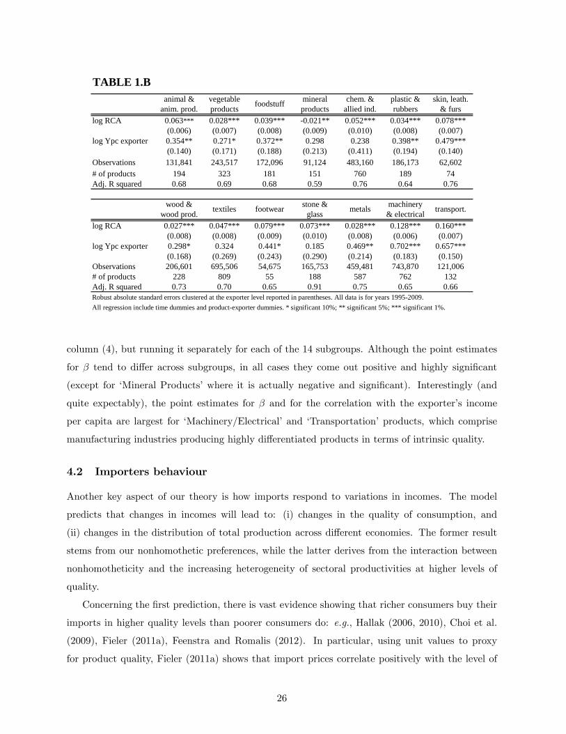
separate subgroups at the 2-digit level.25 In Table 1.B, we repeat the regression conducted in

22For a discussion of the possible sources of bias and direction of bias in similar contexts, see Kugler and Verhoogen

(2012, p. 315), and Manova and Zhang (2012, p. 415).

23Kugler and Verhoogen (2012) use �rm-level data from manufacturing Colombian �rms to regress the unit values

on the total value of output of the �rm. To deal with the measurement error bias, they instrument total output by

the level of total employment of the �rm, which is arguably subject to less measurement error.

24We have also run a two-stage least square regression using the lagged value of the revealed comparative advantage

as instrument (i.e., instrumenting RCAz;x;t by RCAz;x;t�1). This regression, which is available from the authors

upon request, also yields a positive and highly signi�cant coe¢ cient for the correlation of interest.25The subgroups in Table 1.B are formed by merging together subgroups at 2-digit aggregation level, according

to http://www.foreign-trade.com/reference/hscode.htm. We excluded all products within the subgroups �Miscella-

neous�and �Service�.

25

animal & vegetable mineral chem. & plastic & skin, leath.anim. prod. products products allied ind. rubbers & furs

log RCA 0.063*** 0.028*** 0.039*** ­0.021** 0.052*** 0.034*** 0.078***(0.006) (0.007) (0.008) (0.009) (0.010) (0.008) (0.007)

log Ypc exporter 0.354** 0.271* 0.372** 0.298 0.238 0.398** 0.479***(0.140) (0.171) (0.188) (0.213) (0.411) (0.194) (0.140)

Observations 131,841 243,517 172,096 91,124 483,160 186,173 62,602# of products 194 323 181 151 760 189 74Adj. R squared 0.68 0.69 0.68 0.59 0.76 0.64 0.76

wood & stone & machinerywood prod. glass & electrical

log RCA 0.027*** 0.047*** 0.079*** 0.073*** 0.028*** 0.128*** 0.160***(0.008) (0.008) (0.009) (0.010) (0.008) (0.006) (0.007)

log Ypc exporter 0.298* 0.324 0.441* 0.185 0.469** 0.702*** 0.657***(0.168) (0.269) (0.243) (0.290) (0.214) (0.183) (0.150)

Observations 206,601 695,506 54,675 165,753 459,481 743,870 121,006# of products 228 809 55 188 587 762 132Adj. R squared 0.73 0.70 0.65 0.91 0.75 0.65 0.66Robust absolute standard errors clustered at the exporter level reported in parentheses. All data is for years 1995­2009.All regression include time dummies and product­exporter dummies. * significant 10%; ** significant 5%; *** significant 1%.

textiles footwear metals transport.

foodstuff

TABLE 1.B

column (4), but running it separately for each of the 14 subgroups. Although the point estimates

for � tend to di¤er across subgroups, in all cases they come out positive and highly signi�cant

(except for �Mineral Products�where it is actually negative and signi�cant). Interestingly (and

quite expectably), the point estimates for � and for the correlation with the exporter�s income

per capita are largest for �Machinery/Electrical�and �Transportation�products, which comprise

manufacturing industries producing highly di¤erentiated products in terms of intrinsic quality.

4.2 Importers behaviour

Another key aspect of our theory is how imports respond to variations in incomes. The model

predicts that changes in incomes will lead to: (i) changes in the quality of consumption, and

(ii) changes in the distribution of total production across di¤erent economies. The former result

stems from our nonhomothetic preferences, while the latter derives from the interaction between

nonhomotheticity and the increasing heterogeneity of sectoral productivities at higher levels of

quality.

Concerning the �rst prediction, there is vast evidence showing that richer consumers buy their

imports in higher quality levels than poorer consumers do: e.g., Hallak (2006, 2010), Choi et al.

(2009), Fieler (2011a), Feenstra and Romalis (2012). In particular, using unit values to proxy

for product quality, Fieler (2011a) shows that import prices correlate positively with the level of

26

income per head of the importer, even when looking at products originating from the same exporter

and HS-6 category.

The previous literature linking import prices and the importer�s GDP per head has then pro-

vided evidence consistent with the hypothesis that richer individuals purchase goods in higher

quality levels. However, that literature has mostly remained silent as to where those imports tend

to originate from. In that regard, our model also yields an interesting prediction regarding imports

specialisation: if it is true that taste for quality rises with income and comparative advantages

deepen at higher levels of quality, then richer countries should purchase a larger share of their

imports of given goods from economies displaying a comparative advantage in those goods.

In what follows we aim at providing evidence of such relationship between importer�s income per

head and origin of imports. (For computational purposes, given the large number of observations,

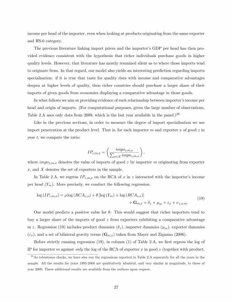
Table 2.A uses only data from 2009, which is the last year available in the panel.)26

Like in the previous sections, in order to measure the degree of import specialisation we use

import penetration at the product level. That is, for each importer m and exporter x of good z in

year t, we compute the ratio:

IPz;m;x =

�impoz;m;xPx2X impoz;m;x

�;

where impoz;m;x denotes the value of imports of good z by importer m originating from exporter

x, and X denotes the set of exporters in the sample.

In Table 2.A, we regress IPz;m;x on the RCA of x in z interacted with the importer�s income

per head (Ym). More precisely, we conduct the following regression:

log (IPz;m;x) = � log (RCAz;x) + � [log (Ym)� log (RCAz;x)]

+Gm;x + �z + �m + "x + �z;x;m:(19)

Our model predicts a positive value for �. This would suggest that richer importers tend to

buy a larger share of the imports of good z from exporters exhibiting a comparative advantage

in z. Regression (19) includes product dummies (�z), importer dummies (�m), exporter dummies

("x), and a set of bilateral gravity terms (Gm;x) taken from Mayer and Zignano (2006).

Before strictly running regression (19), in column (1) of Table 2.A, we �rst regress the log of

IP for importer m against only the log of the RCA of exporter x in good z (together with product,

26As robustness checks, we have also run the regressions reported in Table 2.A separately for all the years in the

sample. All the results for years 1995-2008 are qualitatively identical, and very similar in magnitude, to those of

year 2009. These additional results are available from the authors upon request.

27

importer and exporter dummies), which shows as we would expect that those two variables are

positively correlated. Secondly, in column (2), we report the results of the regression that includes

the interaction term. We can see that the estimated � is positive and highly signi�cant, consistent

with our theory. Finally, in column (3), we add six traditional gravity terms, and we can observe

the previous results remain essentially intact. We can also observe that the estimates for each of

the gravity terms are signi�cant, and they all carry the expected sign.

Notice that regression (19) includes exporter �xed e¤ects ("x). This implies that our regressions

are actually comparing di¤erent degrees of export specialisation across products and destinations

for a given exporter.27 As such, exporter dummies would take care of the possibility that our

estimates may be spuriously capturing the fact the a country with higher total factor productivity

will be commanding larger market shares and specialising more strongly in higher qualities varieties

of goods, which are exactly the types of varieties purchased by richer importers.

Simultaneity of RCA and import penetration

One possible concern with regression (19) is the fact that RCAz;x is computed with the same data

that is used to construct IPz;m;x. In terms of our estimation of �, this could represent an issue

if a very large economy turns out to be also very rich (for example, the case of the US). In that

case, since the imports of good z by such sizable and rich economy will be strongly in�uencing the

independent variableRCAz;x, we may be somehow generating by construction a positive correlation

between IPz;m;x and [log (Ym)� log (RCAz;x)].

In order to deal with this concern, in column (4) we split the set of 184 importers in two

separate subsets of 92 importers each (subset A and subset B). When splitting the original set of

184 importers, we do so in such a way the two subsets display similar GDP per capita distributions.

(See Appendix C for details and descriptive statistics of the two sub-samples.) We next use

the subset A to compute the revealed comparative advantage of each exporter in each product

(RCAz;x), while we use the subset B for IPz;m;x. By construction, there is therefore no link

between IPz;m;x and RCAz;x, since those two variable are computed with data from di¤erent sets

of importers.

As we may readily observe, the results in column (4) of Table 2.A con�rm our previous results

in column (3) �the estimate for � is positive and highly signi�cant, and of very similar magnitude

as in column (3). Lastly, in column (5) we use the RCA computed with the subset A of importers to

27Notice that since Table 2.A is using only data from year 2009 the exporter dummies are also implicitly capturing

the e¤ect of the exporter GDP per head in 2009.

28

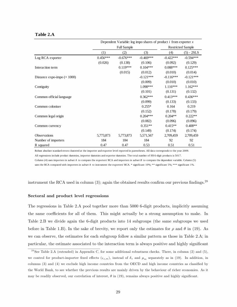
Table 2.A

(1) (2) (3) (4) (5) ­ 2SLSLog RCA exporter 0.456*** ­0.676*** ­0.469*** ­0.422*** ­0.594***

(0.026) (0.138) (0.106) (0.092) (0.129)Interaction term 0.119*** 0.104*** 0.088*** 0.125***

(0.015) (0.012) (0.010) (0.014)Distance expo­impo (× 1000) ­0.121*** ­0.116*** ­0.121***

(0.009) (0.010) (0.010)Contiguity 1.098*** 1.116*** 1.162***

(0.101) (0.131) (0.132)Common official language 0.362*** 0.413*** 0.436***

(0.099) (0.133) (0.133)Common coloniser 0.255* 0.164 0.219

(0.152) (0.178) (0.179)Common legal origin 0.204*** 0.204** 0.222**

(0.082) (0.096) (0.096)Common currency 0.351** 0.415** 0.408**

(0.149) (0.174) (0.174)Observations 5,773,873 5,773,873 5,571,567 2,709,459 2,709,459Number of importers 184 184 184 92 92R squared 0.47 0.47 0.53 0.51 0.51Robust absolute standard errors clustered at  the importer and exporter level reported in parentheses. All data corresponds to the year 2009.

All regressions include product dummies, importer dummies and exporter dummies. The total number of HS 6­digit products is 5017.

Column (4) uses importers in subset A  to compute the exporters' RCA and importers in subset B  to compute the dependent variable. Column (5)

uses the RCA computed with importers in subset A  to instrument the exporters' RCA. * significant 10%; ** significant 5%; *** significant 1%.

Restricted SampleDependent Variable: log impo shares of product i  from exporter x

Full Sample

instrument the RCA used in column (3); again the obtained results con�rm our previous �ndings.28

Sectoral and product level regressions

The regressions in Table 2.A pool together more than 5000 6-digit products, implicitly assuming

the same coe¢ cients for all of them. This might actually be a strong assumption to make. In

Table 2.B we divide again the 6-digit products into 14 subgroups (the same subgroups we used

before in Table 1.B). In the sake of brevity, we report only the estimates for � and � in (19). As

we can observe, the estimates for each subgroup follow a similar pattern as those in Table 2.A; in

particular, the estimate associated to the interaction term is always positive and highly signi�cant

28See Table 2.A (extended) in Appendix C, for some additional robustness checks. There, in column (2) and (5),

we control for product-importer �xed e¤ects (&z;m), instead of �z and �m separately as in (19). In addition, in

columns (3) and (4) we exclude high income countries from the OECD and high income countries as classi�ed by

the World Bank, to see whether the previous results are mainly driven by the behaviour of richer economies. As it

may be readily observed, our correlation of interest, � in (19), remains always positive and highly signi�cant.

29

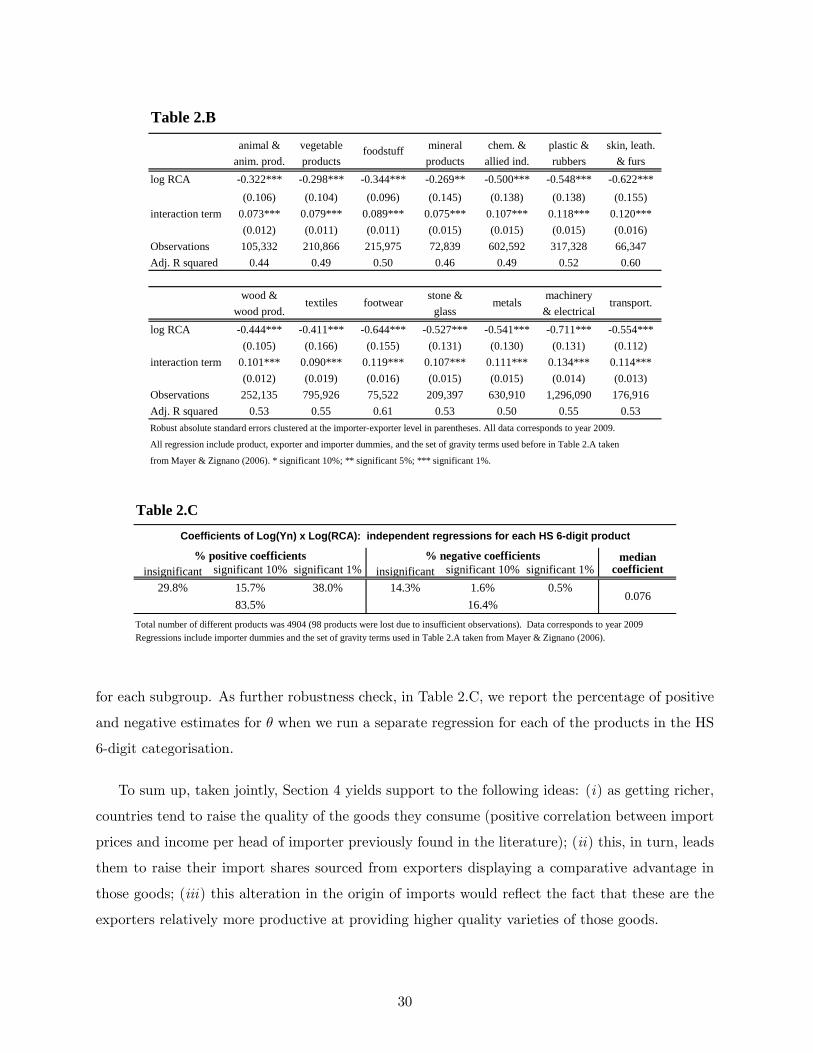
Table 2.B

animal & vegetable mineral chem. & plastic & skin, leath.anim. prod. products products allied ind. rubbers & furs

log RCA ­0.322*** ­0.298*** ­0.344*** ­0.269** ­0.500*** ­0.548*** ­0.622***(0.106) (0.104) (0.096) (0.145) (0.138) (0.138) (0.155)

interaction term 0.073*** 0.079*** 0.089*** 0.075*** 0.107*** 0.118*** 0.120***(0.012) (0.011) (0.011) (0.015) (0.015) (0.015) (0.016)

Observations 105,332 210,866 215,975 72,839 602,592 317,328 66,347Adj. R squared 0.44 0.49 0.50 0.46 0.49 0.52 0.60

wood & stone & machinerywood prod. glass & electrical

log RCA ­0.444*** ­0.411*** ­0.644*** ­0.527*** ­0.541*** ­0.711*** ­0.554***(0.105) (0.166) (0.155) (0.131) (0.130) (0.131) (0.112)

interaction term 0.101*** 0.090*** 0.119*** 0.107*** 0.111*** 0.134*** 0.114***(0.012) (0.019) (0.016) (0.015) (0.015) (0.014) (0.013)

Observations 252,135 795,926 75,522 209,397 630,910 1,296,090 176,916Adj. R squared 0.53 0.55 0.61 0.53 0.50 0.55 0.53Robust absolute standard errors clustered at the importer­exporter level in parentheses. All data corresponds to year 2009.

All regression include product, exporter and importer dummies, and the set of gravity terms used before in Table 2.A taken

from Mayer & Zignano (2006). * significant 10%; ** significant 5%; *** significant 1%.

foodstuff

metals transport.textiles footwear

Table 2.C

medianinsignificant significant 10% significant 1% insignificant significant 10% significant 1% coefficient

Total number of different products was 4904 (98 products were lost due to insufficient observations).  Data corresponds to year 2009Regressions include importer dummies and the set of gravity terms used in Table 2.A taken from Mayer & Zignano (2006).

Coefficients of Log(Yn) x Log(RCA):  independent regressions for each HS 6­digit product

0.0761.6%

% positive coefficients % negative coefficients

83.5% 16.4%29.8% 15.7% 38.0% 14.3% 0.5%

for each subgroup. As further robustness check, in Table 2.C, we report the percentage of positive

and negative estimates for � when we run a separate regression for each of the products in the HS

6-digit categorisation.

To sum up, taken jointly, Section 4 yields support to the following ideas: (i) as getting richer,

countries tend to raise the quality of the goods they consume (positive correlation between import

prices and income per head of importer previously found in the literature); (ii) this, in turn, leads

them to raise their import shares sourced from exporters displaying a comparative advantage in

those goods; (iii) this alteration in the origin of imports would re�ect the fact that these are the

exporters relatively more productive at providing higher quality varieties of those goods.

30

5 Conclusion

We presented a Ricardian model of trade with the distinctive feature that comparative advantages

reveal themselves gradually over the course of development. The key factors behind this process

are the individuals�upgrading in quality of consumption combined with productivity di¤erentials

that widen up as countries seek to increase the quality of their production. As incomes grow

and wealthier consumers raise the quality of their consumption baskets, cost di¤erentials between

countries become more pronounced. The emergence of such heterogeneities, in turn, alters trade

�ows, as each economy gradually specialises in producing the subset of goods for which they enjoy

a rising comparative advantage.

Our model yielded a number of implications that �nd empirical support. In this respect, using

bilateral trade data at the product level, we showed that the share of imports originating from

exporters more intensely specialised in a given product correlates positively with GDP per head

of the importer. This is consistent with the model�s prediction that richer consumers tend to

buy a larger share of their consumption of speci�c goods from countries exhibiting a comparative

advantage in those goods. We also provided some evidence supporting the central assumption

of our model, namely the intensi�cation of comparative advantage at higher quality levels. In

particular, we found that the degree of export specialisation of countries in speci�c goods and the

level of quality of their exports display a positive correlation. This fact is consistent with the idea

that Ricardian specialisation tends to become more intense at the upper levels of quality.

As a last remark, our model has assumed away any sort of trade frictions. In a sense, this

was a deliberate choice, so as to illustrate our proposed mechanism as cleanly as possible. Yet,

incorporating trade costs could actually represent a promising extension to the core model. In

this respect, owing to the widening of productivity di¤erentials at higher quality of production,

a natural implication of the model would be that trade costs will generate milder distortions on

trade �ows as the quality of production rises. This implication could help rationalizing some

empirical observations found in the trade literature, such as the positive relationship between the

imports/GDP ratio and the importer�s GDP per head.

31

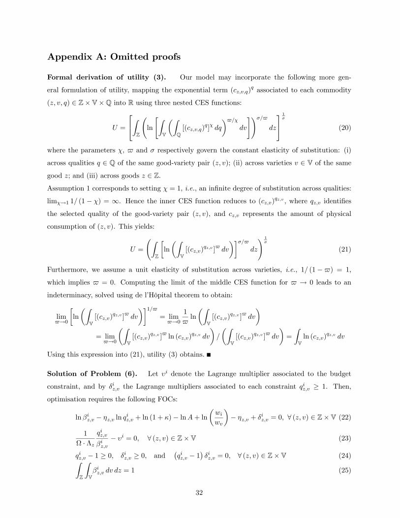
Appendix A: Omitted proofs

Formal derivation of utility (3). Our model may incorporate the following more gen-

eral formulation of utility, mapping the exponential term (cz;v;q)q associated to each commodity

(z; v; q) 2 Z� V�Q into R using three nested CES functions:

U =

24ZZ

ln

"ZV

�ZQ[(cz;v;q)

q]� dq

�$=�dv

#!�=$dz

35 1�

(20)

where the parameters �, $ and � respectively govern the constant elasticity of substitution: (i)

across qualities q 2 Q of the same good-variety pair (z; v); (ii) across varieties v 2 V of the same

good z; and (iii) across goods z 2 Z.

Assumption 1 corresponds to setting � = 1, i.e., an in�nite degree of substitution across qualities:

lim�!1 1= (1� �) = 1. Hence the inner CES function reduces to (cz;v)qz;v , where qz;v identi�es

the selected quality of the good-variety pair (z; v), and cz;v represents the amount of physical

consumption of (z; v). This yields:

U =

ZZ

�ln

�ZV[(cz;v)

qz;v ]$ dv

���=$dz

! 1�

(21)

Furthermore, we assume a unit elasticity of substitution across varieties, i.e., 1= (1�$) = 1,

which implies $ = 0. Computing the limit of the middle CES function for $ ! 0 leads to an

indeterminacy, solved using de l�Hôpital theorem to obtain:

lim$!0

�ln

�ZV[(cz;v)

qz;v ]$ dv

��1=$= lim$!0

1

$ln

�ZV[(cz;v)

qz;v ]$ dv

�= lim$!0

�ZV[(cz;v)

qz;v ]$ ln (cz;v)qz;v dv

�=

�ZV[(cz;v)

qz;v ]$ dv

�=

ZVln (cz;v)

qz;v dv

Using this expression into (21), utility (3) obtains.

Solution of Problem (6). Let �i denote the Lagrange multiplier associated to the budget

constraint, and by �iz;v the Lagrange multipliers associated to each constraint qiz;v � 1. Then,

optimisation requires the following FOCs:

ln�iz;v � �z;v ln qiz;v + ln (1 + �)� lnA+ ln�wiwv

�� �z;v + �iz;v = 0; 8 (z; v) 2 Z� V (22)

1

� �zqiz;v

�iz;v� �i = 0; 8 (z; v) 2 Z� V (23)

qiz;v � 1 � 0, �iz;v � 0, and�qiz;v � 1

��iz;v = 0, 8 (z; v) 2 Z� V (24)Z

Z

ZV�iz;v dv dz = 1 (25)

32

where:

�(Z

Z

"ZVqiz;v ln

1 + �

A

�iz;v�qiz;v��z;v wiwv

!dv

#�dz

)��1�

�z �"Z

Vqiz;v ln

1 + �

A

�iz;v�qiz;v��z;v wiwv

!dv

#1��Note that, although �z in (23) are indexed by z, in the optimum all �z will turn out to be equal.

Hence, we may write that, in the optimum, �z = � for all z.29 Using then the fact that �z = �

for all z, we can next de�ne:

�i � ( � �) �i;

which in turn allows us to re-write (23) as qiz;v = �i�iz;v. Hence, integrating both sides of the

equation over Z and V, and making use of (25), we may obtain:ZZ

ZVqiz;v dv dz = �

i; (26)

which in turn implies that:

�iz;v =qiz;v�i: (27)

Notice also that �i � 1, since qiz;v � 1 and both Z and V have unit mass.

Proof of Lemma 1. Let�s �rst show that when wv = w for all v 2 V and unit labour requirements

are given by (1), then none of the constraints qz;v � 1 of (6) binds in the optimum. For this, note

that given the expressions in (22) and (27), whenever wv = w for all v 2 V, it must be the case that

qiz0;v0 � qiz00;v00 , �z0;v0 � �z00;v00 . Thus, if in the optimum qiz00;v00 > 1 holds for a (z00; v00) 2 Z�V with

�z00;v00 = �, then qiz;v > 1 must be true for all (z; v) 2 Z�V. Then, in order to prove that qiz;v > 1

holds for all (z; v) 2 Z� V, it su¢ ces to prove the following: even when all �z;v = �, except for a

single (zero-mass) good-variety (z00; v00) for which �z00;v00 = �, the optimisation problem (6) yields

qiz00;v00 > 1. If this is the case, then qiz00;v00 > 1 will actually hold true for any distribution of the

productivity draws �z;v with support in the interval��; ��, which includes the uniform distribution

as one special case.

29The result �z = � for all z stems from the assumed iid draws of �z;v with a continuum of countries and goods.

The combination of these assumptions implies that all goods z will display (ex post) an identical distribution of

�z;v over the space of countries v. Such ex post symmetry in the distribution of �z;v across goods, in turn, leads

consumers to optimally set �z = � for all z.

33

When all �z;v = �, except for a single (zero-mass) (z00; v00) with �z00;v00 = �, it follows that when

qz00;v00 = 1:

qiz;v = e� �

��1

�1 + �

A�i

� 1��1

; for all (z; v) 2 Z� V other than�z00; v00

�: (28)

Since the set Z� V has unit mass, integrating (28) across the space Z and V, we obtain �i =

e��=(��1)�(1 + �) =

�A�i

��1=(��1), which in turn yields:�i =

1

e

�1 + �

A

� 1�

: (29)

Now, plugging (29) into (22) and (27), computed for (z00; v00), while using the fact that �iz00;v00 = 1=�i

when qiz00;v00 = 1, we get:

ln (1 + �)� lnA� [ln (1 + �)� lnA] =� + ln e� � + �iz00;v00 = 0: (30)

Hence, considering the de�nition of A � e��(��1)=(��1), (30) reduces to

ln (1 + �) + �iz00;v00�

� � 1 = 0: (31)

However, (31) cannot be true for any � > 0: As a consequence, it must be true that qz00;v00 > 1 for

all � > 0, implying in turn that qz;v > 1 must hold (z; v) 2 Z � V under any distribution of �z;vwith support within the interval

��; ��when wv = w for all v 2 V.

Now, taking into account the above result, we can use (26), (27) and (22), setting �iz;v = 0 for all

(z; v) 2 Z� V, to obtain (7) and (8).

Finally, note that, when wv = w for all v 2 V, using again (22) leads to ln (1 + �)� lnA� ln�i =

�z;v+��z;v � 1

�ln qiz;v for all (z; v) 2 Z�V. De�ning now �i(�) � ln (1 + �)� lnA� ln�i, we can

observe that:@�i

@�=

��z;v � 1

�qiz;v

@qiz;v@�

: (32)

But, given that��z;v � 1

�> 0, then all @qiz;v=@� must necessarily carry the same sign. Suppose

then that @qiz;v=@� � 0, for all (z; v) 2 Z � V. Recalling (26), it follows that @�i=@� � 0 as well.

But, since @�i=@� = (1 + �)�1���i��1

@�i=@�, the fact that @�i=@� � 0 implies that @�i=@� > 0,

which in turn contradicts the fact that @qiz;v=@� � 0 for all (z; v) 2 Z�V. As a result, it must be

the case that @qiz;v=@� > 0 for all (z; v) 2 Z� V.

Proof of Proposition 1. Existence of equilibrium: As a �rst step, we prove that wv = w for all

v 2 V is an equilibrium of the model. Firstly, notice that when wi = w for all i 2 V, the Lagrange

34

multipliers will be identical for all countries, and in particular we may write �i = � for all i 2 V.

Secondly, using Lemma 1, when wv = w for all v 2 V, conditions in (22) together with (27) and

�i = � for all i 2 V, lead to:

qiz;v = qz;v =

�1 + �

Ae�z;v�

�1=(�z;v�1); (33)

�iz;v = �z;v =

�1 + �

A (e�)�z;v

�1=(�z;v�1): (34)

Now, recall that each �z;v is drawn from from an independent uniform probability distribution with

support��; ��. Hence, by the law of large numbers, for each country v 2 V, the (in�nite) sequence

of draws��z;v

z2Z will also be uniformly distributed over

��; ��along the goods space. This

implies that, integrating over Z and bearing in mind (34),RZ �

iz;v dz =

RZ �z;v dz = �v = � > 0, for

each good v 2 V. Next, replacingRZ �

iz;v dz = � into (25), and swapping the order of integration,

we obtainRV � dv = 1, which in turn implies that � = 1 since V has unit mass. Then, it is easy to

check that all conditions (9) hold simultaneously when wv = w for all v 2 V.

Equilibrium uniqueness: We now proceed to prove the above equilibrium is unique. Normalise

w = 1, and suppose for a subset J � V of countries with measure �j > 0 we have wj > 1, while

for a (disjoint) subset K � V of countries with measure �k > 0 we have wk < 1. Denote �nally

by I � V the (complementary) subset of countries with wi = 1. Consider some k 2 K, i 2 I, and

j 2 J , and take (zk; k) ; (zi; i) ; (zj ; j) such that: �zk;k = �zi;i = �zj ;j = �. Notice that, due to the

law of large numbers, for any � 2��; ��the measure of good-variety couples for which the last

condition is satis�ed is the same in k, i and j.

As a �rst step, take country i 2 I. (22) and (23) imply that, for (zk; k), (zi; i) and (zj ; j), we must

have, respectively:

ln (1 + �)� lnA = � ln��i�+ ln (wk) + (� � 1) ln(�izk;k) + � � �

izk;k

= � ln��i�+ (� � 1) ln(�i

zi;i) + � � �izi;i

= � ln��i�+ ln (wj) + (� � 1) ln(�izj ;j ) + � � �

izj ;j :

Notice also from (24) and (27) that if �iz;v > 0, then ln�iz;v= � ln�i, whereas if �iz;v = 0, then

ln�iz;v� � ln�i. Then, �i

zk;k� �i

zi;i� �i

zj ;j.

As a second step, take country k 2 K. (22) and (23) imply that, for (zk; k), (zi; i) and (zj ; j), we

35

must have, respectively:

ln (1 + �)� lnA = � ln(�k) + (� � 1) ln(�kzk;k) + � � �kzk;k

= � ln(�k) + ln

�1

wk

�+ (� � 1) ln(�k

zi;i) + � � �kzi;i

= � ln(�k) + ln

�wjwk

�+ (� � 1) ln(�k

zj ;j) + � � �kzj ;j :

Following an analogous reasoning as before, it follows that �kzk;k

� �kzi;i� �k

zj ;j.

As a third step, take country j 2 J , and notice wj > 1. (22) and (23) imply that, for (zk; k), (zi; i)

and (zj ; j), we must have, respectively:

ln (1 + �)� lnA = � ln��j�+ ln

�wkwj

�+ (� � 1) ln(�j

zk;k) + � � �jzk;k

= � ln��j�+ ln

�1

wj

�+ (� � 1) ln(�j

zi;i) + � � �jzi;k

= � ln��j�+ (� � 1) ln(�j

zj ;j) + � � �jzj ;j :

Again, an analogous reasoning as in the previous cases leads to �jzk;k

� �jzi;i� �j

zj ;j:

Finally, integrate among the good space Z and country space V. The above results lead to:

�jwj

ZZ�jz;kdz + �kwk

ZZ�kz;kdz +

�1� �j � �k

� ZZ�iz;kdz �

�jwj

ZZ�jz;idz + �kwk

ZZ�kz;idz +

�1� �j � �k

� ZZ�iz;idz �

�jwj

ZZ�jz;jdz + �kwk

ZZ�kz;jdz +

�1� �j � �k

� ZZ�iz;jdz:

(35)

Note that the �rst line in (35) equals the world spending on commodities produced in k, the second

equals the world spending on commodities produced in i, and the third equals the world spending

on commodities produced in j. However, when wk < 1 < wj , those inequalities are inconsistent

with market clearing conditions (9). As a result, there cannot exist an equilibrium with measure

�j > 0 of countries with wj > 1 and/or a measure �k > 0 of countries with wk < 1.

Proof of Proposition 2. Preliminarily, notice that (26) together with (27) yields:

�z0;v0 =qz0;v0R

ZRV qz00;v00 dv

00 dz00: (36)

Part (i). From (22), together with Lemma 1 and Proposition 1, we have:��z;v � 1

�ln qz;v + �z;v = ln (1 + �)� lnA� ln�; (37)

thus, computing (37) for any pair of commodities (z0; v0) ; (z00; v00) 2 Z� V yields:��z0;v0 � 1

�ln qz0;v0 + �z0;v0 =

��z00;v00 � 1

�ln qz00;v00 + �z00;v00 : (38)

36

Hence, (38) implies that qz0;v0 > qz00;v00 () �z0;v0 < �z00v00 . By considering this result in conjunction

with (36), our claim immediately follows.

Part (ii). Di¤erentiating (38) with respect to � yields:

dqz0;v0

d�=�z00;v00 � 1�z0;v0 � 1

qz0;v0

qz00;v00

dqz00;v00

d�: (39)

Using (26), (37) and (39):

dqz0;v0

d�=

A

1 + �

��z0;v0 � 1qz0;v0

� 1

�

�ZZ

ZV

�z0;v0 � 1�z00;v00 � 1

qz00;v00

qz0;v0dv00 dz00

���1> 0 (40)

Furthermore, from (36), and considering (39) and (40):

d�z0;v0

d�=1

�2dqz0;v0

d�

�ZZ

ZV

��z00;v00 � �z0;v0�z00;v00 � 1

�qz00;v00 dv

00 dz00�

(41)

It is then easy to observe that (39) implies that dqz0;v0=d� > dqz00;v00=d� when �z0;v0 < �z00v00 . By

considering this result in conjunction with (41) our claim immediately follows.

Part iii). From (26), it immediately follows thatZZ

ZV

�d�z;v=d�

�dv dz = 0. Given our result in

part (ii), there must exist a threshold:

� �

ZZ

ZV

��z;vqz;v=

��z;v � 1

��dv dzZ

Z

ZV

�qz;v=

��z;v � 1

��dv dz

associated to a subset of commodities (z; v) 2 Z�V such that d�z;v=d� = 0. Then it immediately

follows that, for any �z0;v0 � �: d�z0;v0=d� � 0; and for any �z00;v00 � �: d�z00;v00=d� � 0. (With

strict inequalities if �z0;v0 < � < �z00;v00 .)

Proof of Proposition 3. We prove the proposition in di¤erent steps. We �rst prove that, if

an equilibrium exists, then for all h 2 H and all l 2 L, it must necessarily be the case that: 1)

wh 6= wl; 2) wh = wH , wl = wL; 3) wH=wL > 1; 4) wH=wL < 1. Lastly, we prove that a

unique equilibrium exists, with: 5) 1 < wH=wL <1.

Preliminarily, consider a generic country i 2 V, and compute the aggregate demand by i for goods

produced in country v 2 V. From the �rst-order conditions, it follows that:

�iz;v = max

(�(1 + �) (wi=wv)

A (e�i)�z;v

� 1�z;v�1

;1

�i

): (42)

Hence, total demand by i for goods produced in h 2 H and in l 2 L are given, respectively by:ZZ�iz;hwi dz = wi

Z �

�max

(�1 + �

A (e�i)�wiwh

�1=(��1);1

�i

)1

� � �d�; for any h 2 H; (43)

37

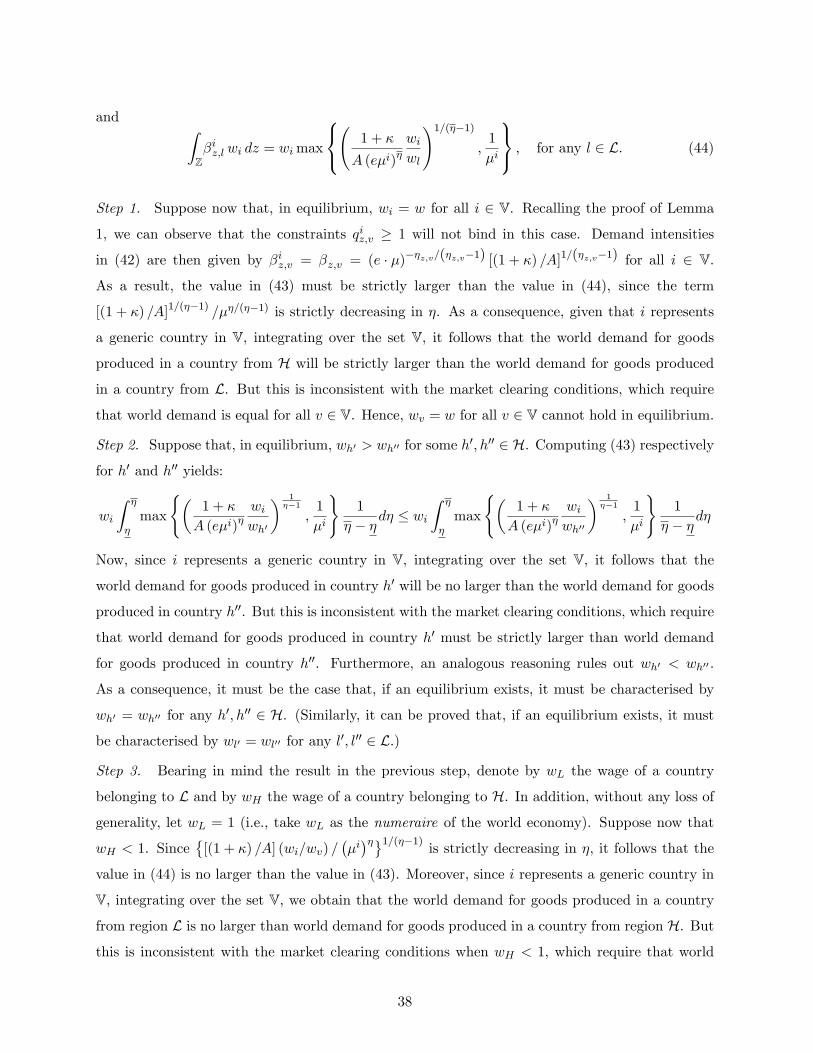
and ZZ�iz;l wi dz = wimax

8<:

1 + �

A (e�i)�wiwl

!1=(��1);1

�i

9=; ; for any l 2 L: (44)

Step 1. Suppose now that, in equilibrium, wi = w for all i 2 V. Recalling the proof of Lemma

1, we can observe that the constraints qiz;v � 1 will not bind in this case. Demand intensities

in (42) are then given by �iz;v = �z;v = (e � �)��z;v=(�z;v�1) [(1 + �) =A]1=(�z;v�1) for all i 2 V.

As a result, the value in (43) must be strictly larger than the value in (44), since the term

[(1 + �) =A]1=(��1) =��=(��1) is strictly decreasing in �. As a consequence, given that i represents

a generic country in V, integrating over the set V, it follows that the world demand for goods

produced in a country from H will be strictly larger than the world demand for goods produced

in a country from L. But this is inconsistent with the market clearing conditions, which require

that world demand is equal for all v 2 V. Hence, wv = w for all v 2 V cannot hold in equilibrium.

Step 2. Suppose that, in equilibrium, wh0 > wh00 for some h0; h00 2 H. Computing (43) respectively

for h0 and h00 yields:

wi

Z �

�max

(�1 + �

A (e�i)�wiwh0

� 1��1

;1

�i

)1

� � �d� � wiZ �

�max

(�1 + �

A (e�i)�wiwh00

� 1��1

;1

�i

)1

� � �d�

Now, since i represents a generic country in V, integrating over the set V, it follows that the

world demand for goods produced in country h0 will be no larger than the world demand for goods

produced in country h00. But this is inconsistent with the market clearing conditions, which require

that world demand for goods produced in country h0 must be strictly larger than world demand

for goods produced in country h00. Furthermore, an analogous reasoning rules out wh0 < wh00 .

As a consequence, it must be the case that, if an equilibrium exists, it must be characterised by

wh0 = wh00 for any h0; h00 2 H. (Similarly, it can be proved that, if an equilibrium exists, it must

be characterised by wl0 = wl00 for any l0; l00 2 L.)

Step 3. Bearing in mind the result in the previous step, denote by wL the wage of a country

belonging to L and by wH the wage of a country belonging to H. In addition, without any loss of

generality, let wL = 1 (i.e., take wL as the numeraire of the world economy). Suppose now that

wH < 1. Since�[(1 + �) =A] (wi=wv) =

��i��1=(��1) is strictly decreasing in �, it follows that the

value in (44) is no larger than the value in (43). Moreover, since i represents a generic country in

V, integrating over the set V, we obtain that the world demand for goods produced in a country

from region L is no larger than world demand for goods produced in a country from region H. But

this is inconsistent with the market clearing conditions when wH < 1, which require that world

38

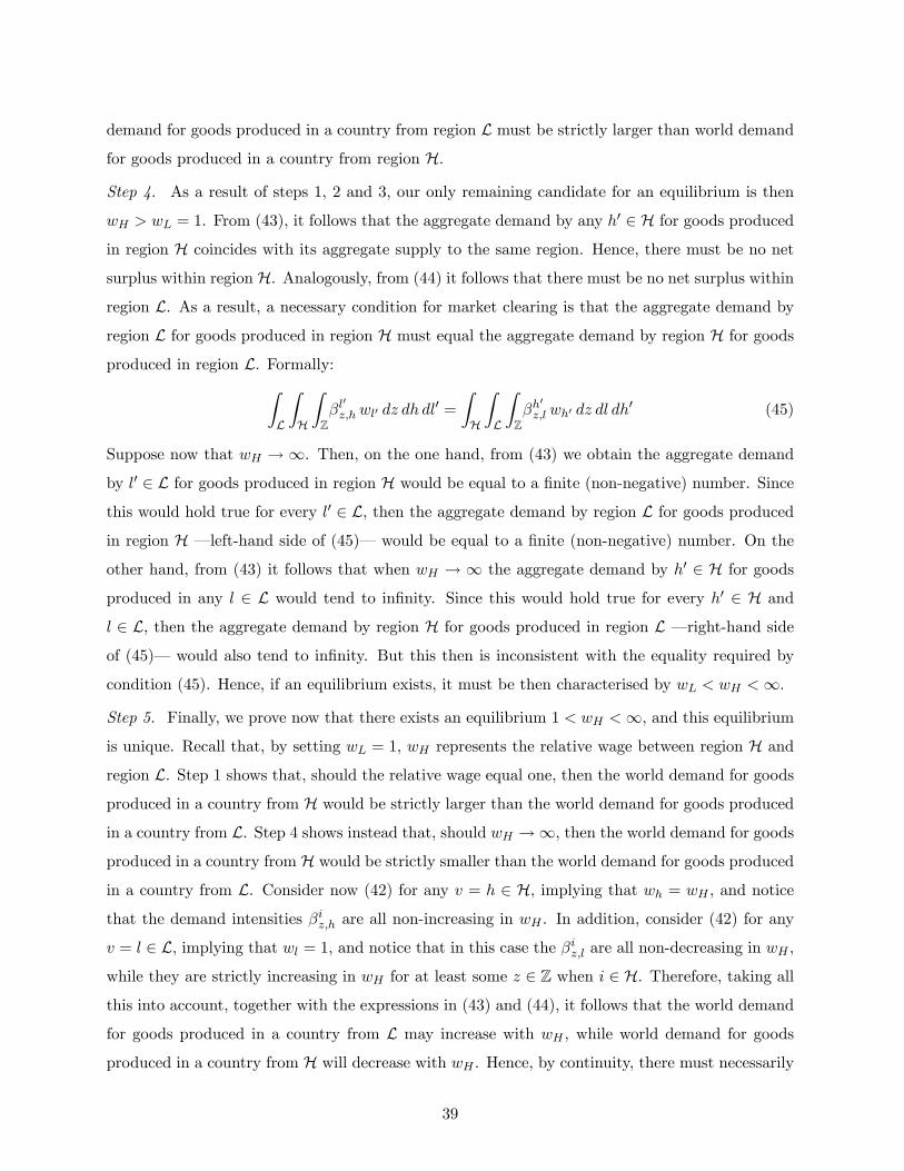
demand for goods produced in a country from region L must be strictly larger than world demand

for goods produced in a country from region H.

Step 4. As a result of steps 1, 2 and 3, our only remaining candidate for an equilibrium is then

wH > wL = 1. From (43), it follows that the aggregate demand by any h0 2 H for goods produced

in region H coincides with its aggregate supply to the same region. Hence, there must be no net

surplus within region H. Analogously, from (44) it follows that there must be no net surplus within

region L. As a result, a necessary condition for market clearing is that the aggregate demand by

region L for goods produced in region H must equal the aggregate demand by region H for goods

produced in region L. Formally:ZL

ZH

ZZ�l

0z;hwl0 dz dh dl

0 =

ZH

ZL

ZZ�h

0z;l wh0 dz dl dh

0 (45)

Suppose now that wH ! 1. Then, on the one hand, from (43) we obtain the aggregate demand

by l0 2 L for goods produced in region H would be equal to a �nite (non-negative) number. Since

this would hold true for every l0 2 L, then the aggregate demand by region L for goods produced

in region H � left-hand side of (45)� would be equal to a �nite (non-negative) number. On the

other hand, from (43) it follows that when wH ! 1 the aggregate demand by h0 2 H for goods

produced in any l 2 L would tend to in�nity. Since this would hold true for every h0 2 H and

l 2 L, then the aggregate demand by region H for goods produced in region L � right-hand side

of (45)� would also tend to in�nity. But this then is inconsistent with the equality required by

condition (45). Hence, if an equilibrium exists, it must be then characterised by wL < wH <1.

Step 5. Finally, we prove now that there exists an equilibrium 1 < wH <1, and this equilibrium

is unique. Recall that, by setting wL = 1, wH represents the relative wage between region H and

region L. Step 1 shows that, should the relative wage equal one, then the world demand for goods

produced in a country from H would be strictly larger than the world demand for goods produced

in a country from L. Step 4 shows instead that, should wH !1, then the world demand for goods

produced in a country from H would be strictly smaller than the world demand for goods produced

in a country from L. Consider now (42) for any v = h 2 H, implying that wh = wH , and notice

that the demand intensities �iz;h are all non-increasing in wH . In addition, consider (42) for any

v = l 2 L, implying that wl = 1, and notice that in this case the �iz;l are all non-decreasing in wH ,

while they are strictly increasing in wH for at least some z 2 Z when i 2 H. Therefore, taking all

this into account, together with the expressions in (43) and (44), it follows that the world demand

for goods produced in a country from L may increase with wH , while world demand for goods

produced in a country from H will decrease with wH . Hence, by continuity, there must necessarily

39

exist some 1 < wH <1 consistent with all market clearing conditions holding simultaneously. In

addition, this equilibrium must then also be unique.

Proof of Proposition 4.

Part (i). From the FOC (22) - (25) we may obtain that for a consumer in any country in

region L the following conditions must hold:

� (� � 1) ln qLL � ln�L + ln (1 + �)� lnA� � + �LL = 0; for all (z; l) 2 Z� L; (46)

���z;h � 1

�ln qLz;h� ln�L+ln (1 + �)� lnA� lnwH��z;h+�Lz;h = 0; for all (z; h) 2 Z�H: (47)

Similarly, for a consumer in any country in region H, it must be true that:

� (� � 1) ln qHL � ln�H + ln (1 + �)� lnA+ lnwH � � + �HL = 0; for all (z; l) 2 Z� L; (48)

���z;h � 1

�ln qHz;h � ln�H + ln (1 + �)� lnA� �z;h + �Hz;h = 0; for all (z; h) 2 Z�H: (49)

Suppose now there exists some (z0; v0) 2 Z � V for which qLz0;v0 > qHz0;v0 . Then, combining either

the pair of equations (46) and (48), or the pair of equations (47) and (49), in both cases we would

obtain that:

ln

��H

�LwH

�=��z0;v0 � 1

�ln

qLz0;v0

qHz0;v0

!+ �Hz0;v0 > 0: (50)

Expression (50) implies, in turn, that 1 < �L < wH�L < �H : From (26), it follows that there must

exist some (z00; v00) 2 Z � V for which qLz00;v00 < qHz00;v00 . Using the same line of reasoning, we now

obtain:

ln��LwH=�

H�=��z00;v00 � 1

�ln�qHz00;v00=q

Lz00;v00

�+ �Lz00;v00 > 0;

which contradicts (50). As a consequence, it must be the case that qHz;v � qLz;v for all (z; v) 2 Z�V.

Now, suppose qHz0;v0 = qLz0;v0 > 1 for some (z0; v0) 2 Z � V. Again, combining either the pair of

equations (46) and (48), or the pair of equations (47) and (49), we obtain:

ln��H=�LwH

�= 0: (51)

Expression (51) implies, in turn, that 1 < �L < wH�L = �H : Hence, there must exist again some

(z00; v00) 2 Z� V for which qLz00;v00 < qHz00;v00 . Using the same line of reasoning, we now obtain:

ln��LwH=�

H�=��z00;v00 � 1

�ln�qHz00;v00=q

Lz00;v00

�> 0;

which contradicts (51). Therefore, it must be true that qHz;v > qLz;v for all (z; v) 2 Z�V, whenever

qHz;v > 1:

40

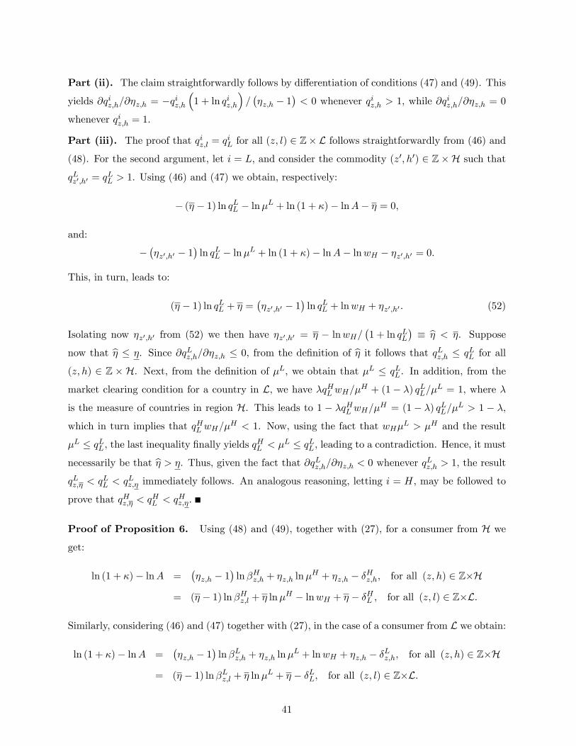
Part (ii). The claim straightforwardly follows by di¤erentiation of conditions (47) and (49). This

yields @qiz;h=@�z;h = �qiz;h�1 + ln qiz;h

�=��z;h � 1

�< 0 whenever qiz;h > 1, while @q

iz;h=@�z;h = 0

whenever qiz;h = 1:

Part (iii). The proof that qiz;l = qiL for all (z; l) 2 Z�L follows straightforwardly from (46) and

(48). For the second argument, let i = L, and consider the commodity (z0; h0) 2 Z�H such that

qLz0;h0 = qLL > 1. Using (46) and (47) we obtain, respectively:

� (� � 1) ln qLL � ln�L + ln (1 + �)� lnA� � = 0;

and:

���z0;h0 � 1

�ln qLL � ln�L + ln (1 + �)� lnA� lnwH � �z0;h0 = 0:

This, in turn, leads to:

(� � 1) ln qLL + � =��z0;h0 � 1

�ln qLL + lnwH + �z0;h0 : (52)

Isolating now �z0;h0 from (52) we then have �z0;h0 = � � lnwH=�1 + ln qLL

�� b� < �. Suppose

now that b� � �. Since @qLz;h=@�z;h � 0, from the de�nition of b� it follows that qLz;h � qLL for all

(z; h) 2 Z � H. Next, from the de�nition of �L, we obtain that �L � qLL. In addition, from the

market clearing condition for a country in L, we have �qHL wH=�H + (1� �) qLL=�L = 1, where �

is the measure of countries in region H. This leads to 1 � �qHL wH=�H = (1� �) qLL=�L > 1 � �,

which in turn implies that qHL wH=�H < 1. Now, using the fact that wH�L > �H and the result

�L � qLL, the last inequality �nally yields qHL < �L � qLL, leading to a contradiction. Hence, it must

necessarily be that b� > �. Thus, given the fact that @qLz;h=@�z;h < 0 whenever qLz;h > 1, the resultqLz;� < q

LL < q

Lz;� immediately follows. An analogous reasoning, letting i = H, may be followed to

prove that qHz;� < qHL < q

Hz;�.

Proof of Proposition 6. Using (48) and (49), together with (27), for a consumer from H we

get:

ln (1 + �)� lnA =��z;h � 1

�ln�Hz;h + �z;h ln�

H + �z;h � �Hz;h, for all (z; h) 2 Z�H

= (� � 1) ln�Hz;l + � ln�H � lnwH + � � �HL , for all (z; l) 2 Z�L:

Similarly, considering (46) and (47) together with (27), in the case of a consumer from L we obtain:

ln (1 + �)� lnA =��z;h � 1

�ln�Lz;h + �z;h ln�

L + lnwH + �z;h � �Lz;h, for all (z; h) 2 Z�H

= (� � 1) ln�Lz;l + � ln�L + � � �LL, for all (z; l) 2 Z�L:

41

Therefore, from the above expressions we may obtain:

�� � �z;h

�ln

��H

�L

�+��LL � �HL

�+��Lz;h � �Hz;h

�=��z;h � 1

�ln�Hz;h

�Lz;h+ (� � 1) ln

�Lz;l

�Hz;l

!: (53)

Notice that �LL � �HL and �Lz;h � �Hz;h, because �LwH > �H . Therefore, since ln��H=�L

�> 0, from

(53) we may obtain that:

�Hz;h=�Lz;h > �

Hz;l=�

Lz;l; whenever �z;h < �;

�Hz;h=�Lz;h � �Hz;l=�Lz;l when �z;h = �:

. (54)

Recall now that @�iz;h=@�z;h < 0 whenever qiz;h > 1, while @�

iz;h=@�z;h = 0 if q

iz;h = 1. In addition,

recall that qHz;h � qLz;h. As a result, using (54), we can observe that for any two pairs (z; h0) and

(z; h00) such that �z;h0 = � < �z;h00 , �Hz;�=�

Lz;� > �Hz;h00=�

Lz;h00 must be true, since q

Hz;� > 1 always

holds. Merging this result with (54) leads to the following chain of inequalities:

�Hz;�

�Lz;�>�Hz;�z;h00

�Lz;�z;h00��Hz;l

�Lz;l: (55)

Now, suppose that �Hz;� � �Lz;�. Then, from (55) it follows that �Hz;v < �Lz;v for all (z; v) 2 Z� V.

However, since in the optimum the budget constraint of a consumer from Lmust hold with equality,

then the fact that �Hz;� � �Lz;� would in turn imply thatRZRV �

Hz;v dv dz <

RZRV �

Lz;v dv dz = 1. But,R

ZRV �

Hz;v dv dz < 1 is inconsistent with consumers maximising behaviour in H. As a consequence,

it must thus be the case that �Hz;� > �Lz;�.

42

Appendix B: Additional theoretical results

Proposition 7 Suppose that the set V is composed by K disjoint subsets, indexed by k = 1; :::;K,

each denoted by Vk � V and with Lebesgue measure �k > 0. Assume that for any country vk 2 Vkeach �z;vk is independently drawn from a uniform distribution with support [�k; �], with �k0 < �k00

for k0 < k00.Then: w1 > ::: > wk0 > ::: > wK , where 1 < k0 < K.

Proof. Combining (22) and (23), yields:

�iz;v = max

(��1 + �

A

��wiwv

��e � �i

���z;v�1=(�z;v�1) ; 1�i

)� �i

��z;v; wv

�: (56)

Notice from (56) that @�i��z;v; wv

�=@�z;v � 0 and @�i

��z;v; wv

�=@wv � 0.

Consider now two generic regions k0 < k00, and suppose that wk0 � wk00 . Since the distribution

of �z;k0 FOSD the distribution of �z;k00 , then it follows thatRZ �

iz;k0dz �

RZ �

iz;k00dz. Moreover,

recalling the proof of Lemma 1 it follows that the �iz;v in (56) must be strictly decreasing in �z;v

and in wv at least in one of all the regions in the world.30 As a result, there will exist a positive

measure of countries for whichRZ �

iz;k0dz >

RZ �

iz;k00dz when wk0 � wk00 . Therefore, integrating

over the set V, we obtain thatRVRZ �

iz;k0dz >

RVRZ �

iz;k00dz. That is, the world demand for goods

produced in a country from region k0 is strictly larger than world demand for goods produced

in a country from region k00. But this is inconsistent with the market clearing conditions when

wk0 � wk00 , which require that world demand for goods produced in a country from region k0 must

be no larger than world demand for goods produced in a country from region k00. As a consequence,

it must be that wk0 > wk00 .

Proposition 8 For country v1 2 V1 such that �z;v1 = � and any country vk 2 Vk such that

�z;vk = �k and k 6= 1: RCAz;v1 > RCAz;vk , for any z 2 Z.

Proof. Countries with identical incomes have identical budget shares. Let �jz;v denote the common

budget share for (z; v) in j. Then, from the de�nition of total production of good z by country v,

we have that Xz;v =PKj=1 �j�

j��z;v; wv

�wj . Notice also that Xv = wv and Wz=W = 1. Hence,

(11) yields:

RCAz;v =

PKj=1 �j�

j��z;v; wv

�wj

wv: (57)

30More precisely, it must be that the �iz;v in (56) are strictly decreasing in �z;v and wv at least in region k�, such

that wk� 2 maxfw1; :::; wKg. That is, the region (or regions) exhibiting with the highest wage.

43

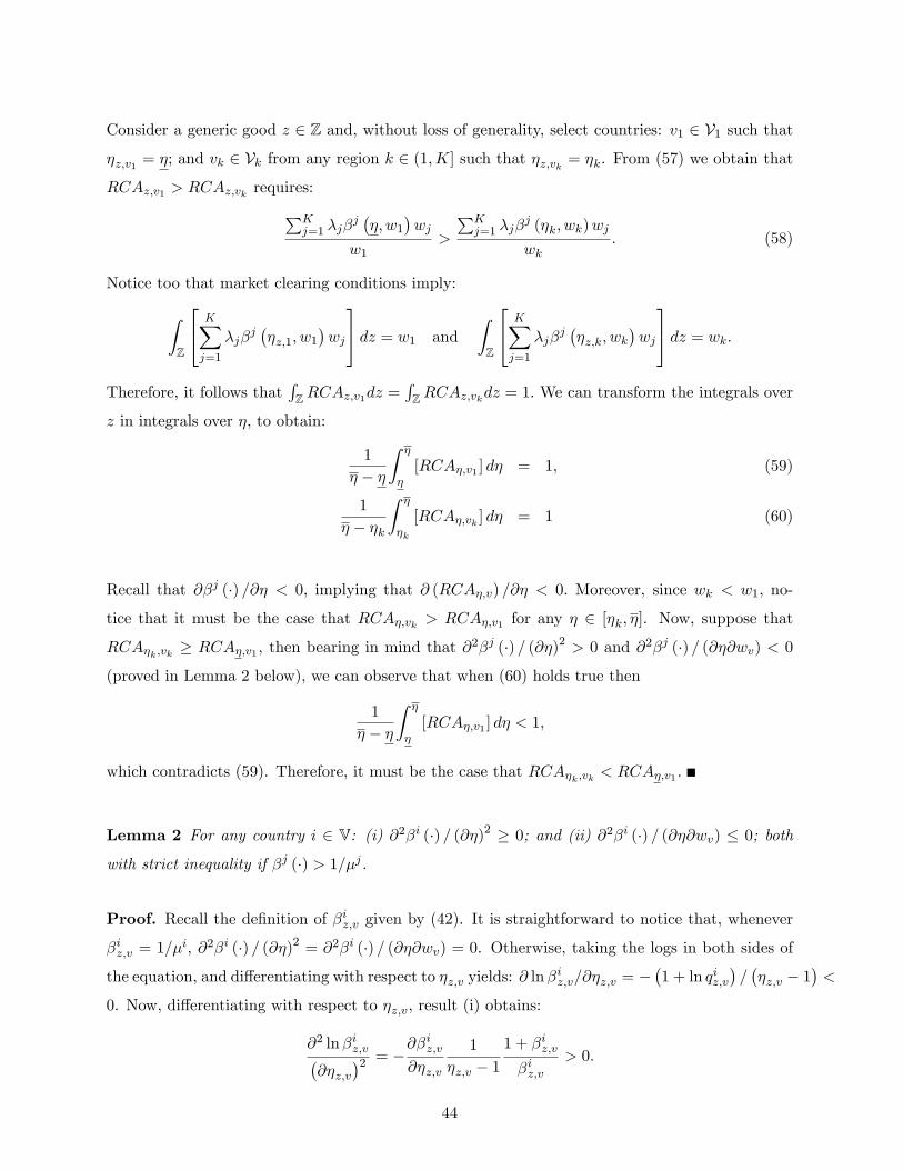
Consider a generic good z 2 Z and, without loss of generality, select countries: v1 2 V1 such that

�z;v1 = �; and vk 2 Vk from any region k 2 (1;K] such that �z;vk = �k. From (57) we obtain that

RCAz;v1 > RCAz;vk requires:PKj=1 �j�

j��; w1

�wj

w1>

PKj=1 �j�

j (�k; wk)wj

wk: (58)

Notice too that market clearing conditions imply:

ZZ

24 KXj=1

�j�j��z;1; w1

�wj

35 dz = w1 andZZ

24 KXj=1

�j�j��z;k; wk

�wj

35 dz = wk:Therefore, it follows that

RZRCAz;v1dz =

RZRCAz;vkdz = 1: We can transform the integrals over

z in integrals over �, to obtain:

1

� � �

Z �

�[RCA�;v1 ] d� = 1; (59)

1

� � �k

Z �

�k

[RCA�;vk ] d� = 1 (60)

Recall that @�j (�) =@� < 0; implying that @ (RCA�;v) =@� < 0: Moreover, since wk < w1; no-

tice that it must be the case that RCA�;vk > RCA�;v1 for any � 2 [�k; �]. Now, suppose that

RCA�k;vk � RCA�;v1 , then bearing in mind that @2�j (�) = (@�)2 > 0 and @2�j (�) = (@�@wv) < 0

(proved in Lemma 2 below), we can observe that when (60) holds true then

1

� � �

Z �

�[RCA�;v1 ] d� < 1;

which contradicts (59). Therefore, it must be the case that RCA�k;vk < RCA�;v1 .

Lemma 2 For any country i 2 V: (i) @2�i (�) = (@�)2 � 0; and (ii) @2�i (�) = (@�@wv) � 0; both

with strict inequality if �j (�) > 1=�j.

Proof. Recall the de�nition of �iz;v given by (42). It is straightforward to notice that, whenever

�iz;v = 1=�i, @2�i (�) = (@�)2 = @2�i (�) = (@�@wv) = 0. Otherwise, taking the logs in both sides of

the equation, and di¤erentiating with respect to �z;v yields: @ ln�iz;v=@�z;v = �

�1 + ln qiz;v

�=��z;v � 1

�<

0. Now, di¤erentiating with respect to �z;v, result (i) obtains:

@2 ln�iz;v�@�z;v

�2 = �@�iz;v@�z;v

1

�z;v � 11 + �iz;v

�iz;v> 0:

44

With regard to result (ii), di¤erentiating with respect to �z;v and wv, we have:

@2 ln�iz;v@�z;v@wv

= � 1

�z;v � 1

@ ln�iz;v@wv

+@ ln�i

@wv

!:

Note that the term in brackets can be rewritten as ��1=wv + @ ln�

i=@wv�=��z;v � 1

�. From the

de�nition of qiz;v:@ ln qiz;v@wv

= � 1

�z;v � 1

�1

wv+@ ln�i

@wv

�� 0:

hence, it must hold 1=wv + @ ln�i=@wv > 0, which in turn implies:

@ ln�iz;v@wv

+@ ln�i

@wv< 0.

Then it straightforwardly follows that @2 ln�iz;v=�@�z;v@wv

�> 0 as claimed.

Proposition 9 Let �jz;� denote the demand intensity by a consumer from country j 2 Vj for the

variety of good z produced in country v1 such that �z;v1 = �. Then: �1z;� > ::: > �

j0z;� > ::: > �

Kz;�,

where 1 < j0 < K.

Proof. Consider a pair of generic consumers from regions j0 and j00, where j0 < j00. In addition,

consider a pair of generic exporters from countries vk0 and vk00 , where k0 � k00. Following an

analogous procedure as in the proof of Proposition 6, combining (22) and (23) of consumers j0 and

j00 for the varieties of good z produced in vk0 and vk00 , we may obtain:��z;vk00 � �z;vk0

�ln��j

0=�j

00�+��j

00z;vk0

� �j0z;vk0�+��j

00z;vk00

� �j0z;vk00�=�

�z;vk0 � 1�ln��j

0z;vk0

=�j00z;vk0

�+��z;vk00 � 1

�ln��j

00z;vk00

=�j0z;vk00

�:

(61)

Since ln��j

0=�j

00�> 0 and �j

00z;vk

� �j0z;vk, from (61) it follows that �j

0z;vk0

=�j00z;vk0

> �j0z;vk00

=�j00z;vk00

when �z;vk0 < �z;vk00 . Now, let k0 = 1 and pick z such that �z;v1 = �. Next, suppose �

j0z;� � �j

00z;�.

Then, we must have that �j0z;v � �j

00z;v for all (z; v) 2 Z� V, with strict inequality for all (z; v)

such that �z;vk > �. However, since the budget constraints of consumer j0 and j00 require thatRZRV �

j0z;v dv dz =

RZRV �

j00z;v dv dz, then �

j0z;� � �j

00z;� cannot possibly be true.

45

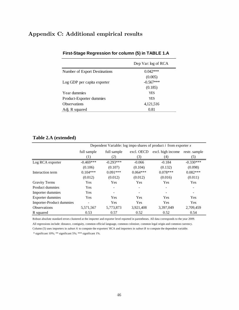
Appendix C: Additional empirical results

First­Stage Regression for column (5) in TABLE 1.A

Number of Export Destinations

Log GDP per capita exporter

Year dummiesProduct­Exporter dummiesObservationsAdj. R squared

Dep Var: log of RCA

YESYES

4,121,5160.81

0.042***(0.005)

­0.567***(0.185)

Table 2.A (extended)

full sample full sample excl. OECD excl. high income restr. sample(1) (2) (3) (4) (5)

Log RCA exporter ­0.469*** ­0.293*** ­0.066 ­0.184 ­0.330***(0.106) (0.107) (0.104) (0.132) (0.098)

Interaction term 0.104*** 0.091*** 0.064*** 0.078*** 0.082***(0.012) (0.012) (0.012) (0.016) (0.011)

Gravity Terms Yes Yes Yes Yes YesProduct dummies Yes ­ ­ ­ ­Importer dummies Yes ­ ­ ­ ­Exporter dummies Yes Yes Yes Yes YesImporter­Product dummies ­ Yes Yes Yes YesObservations 5,571,567 5,773,873 3,921,408 3,397,049 2,709,459R squared 0.53 0.57 0.52 0.52 0.54Robust absolute standard errors clustered at the importer and exporter level reported in parentheses. All data corresponds to the year 2009.

All regressions include: distance, contiguity, common official language, common coloniser, common legal origin and common currency.Column (5) uses importers in subset A  to compute the exporters' RCA and importers in subset B  to compute the dependent variable.

 * significant 10%; ** significant 5%; *** significant 1%.

Dependent Variable: log impo shares of product i  from exporter x

46

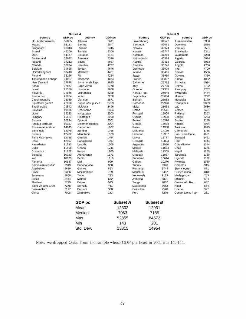
country GDP pc country GDP pc country GDP pc country GDP pcUn. Arab Emirates 52855 Albania 6641 Luxembourg 84572 Turkmenistan 6936Macau 51111 Samoa 6547 Bermuda 52091 Dominica 6580Singapore 47313 Ukraine 6415 Norway 49974 Vanuatu 6531Brunei 46206 Tunisia 6300 Kuwait 46747 El salvador 6341USA 41147 Ecuador 6171 Australia 41288 Guatemala 6288Switzerland 39632 Armenia 5376 Netherlands 40574 Algeria 6074Iceland 37212 Egypt 4957 Austria 37413 Georgia 5063Canada 36234 Namibia 4737 Sweden 35246 Angola 4756Belgium 34625 Jordan 4646 Denmark 33929 Iraq 4709United kingdom 33410 Maldives 4461 Ireland 33406 Bhutan 4566Finland 32186 Fiji 4284 Japan 31980 Guyana 4336Trinidad and Tobago 31057 Indonesia 4074 France 30837 Kiribati 4092New Zealand 27878 Syrian Arab Rep. 3995 Bahamas 28382 Sri lanka 4034Spain 27647 Cape verde 3770 Italy 27709 Bolivia 3792Israel 25559 Honduras 3608 Greece 27305 Paraguay 3702Slovenia 24956 Micronesia 3329 Korea, Rep. 25048 Swaziland 3444Puerto rico 23664 India 3238 Seychelles 23864 Morocco 3292Czech republic 23059 Viet nam 2871 Bahrain 23538 Mongolia 3170Equatorial guinea 22008 Papua new guinea 2753 Barbados 22928 Philippines 2839Saudi arabia 21542 Moldova 2496 Malta 21668 Lao 2636Slovakia 19986 Uzbekistan 2384 Oman 20541 Yemen 2401Libya 19233 Kyrgyzstan 2300 Portugal 19904 Pakistan 2353Hungary 16521 Nicaragua 2190 Cyprus 18998 Congo 2223Estonia 16294 Djibouti 2061 Poland 16376 Sudan 2188Antigua­Barbuda 15047 Solomon islands 2004 Croatia 15084 Nigeria 2034Russian federation 14645 Cameroon 1807 Palau 14988 Tajikistan 1873Saint lucia 13079 Zambia 1765 Lithuania 14189 Cambodia 1768Belarus 12782 Mauritania 1578 Lebanon 12907 Sao Tome­Princ. 1681Saint Kitts­Nevis 12755 Gambia 1464 Latvia 12777 Senegal 1492Chile 12007 Bangladesh 1397 Grenada 12024 Haiti 1444Kazakhstan 11733 Lesotho 1309 Argentina 11960 Cote d'ivoire 1344Cuba 11518 Ghana 1241 Mexico 11634 Chad 1276Costa rica 11227 Kenya 1205 Malaysia 11309 Nepal 1209Bulgaria 10923 Afghanistan 1171 Uruguay 11067 Tanzania, 1189Iran 10620 Benin 1116 Suriname 10644 Uganda 1152Panama 10187 Mali 999 Gabon 10276 Rwanda 1030Dominican republic 9919 Burkina faso 900 Turkey 9920 Comoros 915Azerbaijan 9619 Guinea 823 Romania 9742 Sierra leone 871Brazil 9356 Mozambique 759 Mauritius 9487 Guinea­bissau 818Botswana 8868 Togo 733 Venezuela 9123 Madagascar 753Belize 8444 Malawi 652 Jamaica 8801 Ethiopia 684Thailand 7799 Eritrea 593 Tonga 7862 Central Afr. Rep. 647Saint Vincent­Gren. 7378 Somalia 461 Macedonia 7682 Niger 534Bosnia­Herz. 7117 Burundi 368 Colombia 7528 Liberia 397China 7008 Zimbabwe 143 Peru 7279 Congo, Dem. Rep. 231

Subset A Subset B

GDP pc Subset A Subset BMean 12302 12931Median 7063 7185Max 52855 84572Min 143 231Std. Dev. 13315 14954

Note: we dropped Qatar from the sample whose GDP per head in 2009 was 159,144.

47

References

[1] Alcala, F. (2012). �Specialization Across Goods and Product Quality�, Mimeo, Univ. of Murcia.

[2] Bastos, P. and Silva, J. (2010). �The Quality of a Firm�s Exports: Where you export to matters�,

Journal of International Economics, vol. 82, pp. 99-111.

[3] Bergstrand, J. (1990). �The Heckscher-Ohlin-Samuelson Model, The Linder Hypothesis and the Deter-

minants of Bilateral Intra-Industry Trade�, Economic Journal, vol. 100, pp. 1216-1229.

[4] Brooks, E. (2006). �Why don�t �rms export more? Product quality and Colombian plants�, Journal of

Development Economics, vol. 80, pp. 160-178.

[5] Choi, Y. C., Hummels, D. and Xiang, C. (2009). �Explaining Import Quality: The Role of the Income

Distribution�, Journal of International Economics, vol. 77, pp. 265-275.

[6] Crino, R. and Epifani, P. (2012). �Productivity, Quality and Export Behavior�, Economic Journal, 122,

pp. 1206-1243.

[7] Crozet, M., Head, K. and Mayer, T. (2012). �Quality Sorting and Trade: Firm-level evidence for French

wine�, Review of Economic Studies, vol. 79, pp. 609-644.

[8] Dalgin, M., Trindade, V. and Mitra, D. (2008). �Inequality, Nonhomothetic Preferences, and Trade: A

Gravity Approach�, Southern Economic Journal, vol. 74, pp. 747-774.

[9] Dornbusch, R., Fischer, S. and Samuelson, P. (1977). �Comparative Advantage, Trade, and Payments

in a Ricardian Model with a Continuum of Goods�, American Economic Review, vol. 67, pp. 823-839.

[10] Fajgelbaum, P., Grossman, G. and Helpman, E. (2011). �Income Distribution, Product Quality, and

International Trade�, Journal of Political Economy, vol. 119, pp. 721-765.

[11] Feenstra, R. and Romalis, J. (2012).�International Prices and Endogenous Quality�, NBER Working

Papers 18314.

[12] Flam, H. and Helpman, E. (1987). �Vertical Product Di¤erentiation and North-South Trade�, American

Economic Review, vol. 77, pp. 810-822.

[13] Fieler, A. C. (2011a). �Quality Di¤erentiation in Trade:Theory and Evidence�, Mimeo, U Penn.

[14] Fieler, A. C. (2011b). �Nonhomotheticity and Bilateral Trade: Evidence and a Quantitative Explana-

tion�, Econometrica, vol. 79, pp. 1069-1101.

48

[15] Foellmi, R., Hepenstrick, C. and Zweimuller, J. (2010). �Income E¤ects in the Theory of Monopolistic

Competition and International Trade�, Mimeo, University of Zurich.

[16] Francois, J. and Kaplan, S. (1996). �Aggregate Demand Shifts, Income Distribution, and the Linder

Hypothesis�, Review of Economics and Statistics, vol. 78, pp. 244-250.

[17] Gaulier, G. and Zignago, S. (2010). �BACI: International Trade Database at the Product-level. The

1994-2007 Version�, CEPII Working Paper 2010-23.

[18] Hallak, J. C. (2006). �Product Quality and the Direction of Trade�, Journal of International Economics,

vol. 68, pp. 238-265.

[19] Hallak, J. C. (2010). �A Product-Quality View of the Linder Hypothesis�, Review of Economics and

Statistics, vol. 92, pp. 453-466.

[20] Hallak, J. C., and Schott, P. (2011). �Estimating Cross-Country Di¤erences in Product Quality�, Quar-

terly Journal of Economics, vol. 126, pp. 417-474.

[21] Iacovone, L. and Javorcik, B. (2008). �Shipping Good Tequila out: Investment, Domestic Unit Values

and Entry of Multi-Product Plants into Export Markets�, Mimeo, Oxford University.

[22] Jaimovich, E. and Merella, V. (2012). �Quality Ladders in a Ricardian Model of Trade with Nonhomo-

thetic Preferences�, Journal of the European Economic Association, vol. 10, pp. 908-937.

[23] Kugler, M. and Verhoogen, E. (2012). �Prices, Plant Size, and Product Quality�, Review of Economic

Studies, vol. 79, pp. 307-339,

[24] Khandelwal, A. (2010). �The long and short (of) quality ladders�, Review of Economic Studies, vol. 77,

1450-76.

[25] Linder, S. (1961). An Essay on Trade and Transformation, Uppsala: Almqvist & Wiksell.

[26] Manova, K. and Zhang, Z. (2012). �Export Prices across Firms and Destinations�, Quarterly Journal

of Economics, vol. 127, pp. 379-436.

[27] Matsuyama, K. (2000). �A Ricardian Model with a Continuum of Goods under Nonhomothetic Prefer-

ences: Demand Complementarities, Income Distribution, and North-South Trade�, Journal of Political

Economy, vol. 108, pp. 1093-1120.

[28] Markusen, J. (1986). �Explaining the Volume of Trade: an Eclectic Approach,�American Economics

Review, vol. 76, pp. 1002-1011.

49

[29] Mayer, T. and Zignago, S. (2006). �GeoDist: the CEPII�s Distances and Geographical Database�,

MPRA Paper 31243.

[30] Murphy, K. and Shleifer, A. (1997). �Quality and Trade,�Journal of Development Economics, vol. 53,

pp. 1-15.

[31] Schott, P. (2004). �Across-Product versus within-Product Specialization in International Trade�, Quar-

terly Journal of Economics, vol. 119, pp.647-678.

[32] Simonovska, I. (2011). �Income di¤erences and prices of tradables�, Mimeo, UC Davis.

[33] Stokey, N. (1991). �The Volume and Composition of Trade between Rich and Poor Countries�, Review

of Economic Studies, vol. 58, pp. 63-80.

[34] Tarasov, A. (2012). �Trade Liberalization and Welfare Inequality: a Demand-Based Approach�, Scan-

dinavian Journal of Economics, vol. 114, 1296-1317.

[35] Verhoogen, E. (2008). �Trade, Quality Upgrading and Wage Inequality in the Mexican Manufacturing

Sector�, Quarterly Journal of Economics, vol. 123, pp 489-530.

50