Embed Size (px)
Citation preview
KLIPPEL, E-Learning, training 4 8/15/2014
1
Hands-On Training 4
Loudspeaker Distortion Measurements
1 Objective of the Hands-on Training
- Getting an overview of the important distortion measurement techniques
- Understanding the conditions required to generate dominant nonlinear distortions
- Investigating the influence of the stimulus and the role of the state variables
- Interpreting measurement results (spectral and temporal properties)
- Developing practical skills in performing an accurate measurement
- Optimizing the measurement setup
2 Requirements
2.1 Previous Knowledge of the Participants
It is recommended to do the previous Klippel Trainings before starting this training.
2.2 Minimal Requirements
Participants will need the measurement results provided in the Klippel database Training 4_Loudspeaker
Distortion Measurements.kdbx. For the purpose of this training, there is no requirement to have access to a
Klippel R&D measurement system. The database may be viewed by downloading dB-Lab from
www.klippel.de/training and installing the software on a Windows PC.
2.3 Optional Requirements
If participants have access to a KLIPPEL R&D measurement system, we recommend performing additional
measurements on transducers provided by the instructor or other participants. In order to perform these
measurements, you will also need the following software and hardware components:
Transfer Function Measurement Module (TRF)
3D Distortion Measurement Module (DIS)
Distortion Analyzer DA2
Laser Sensor + Controller
Amplifier
Driver Stand
3 The Training Process
1. Read the introduction.
2. Watch the demo video.
3. Answer the preparatory questions.
4. Follow the instructions to interpret the results in the database and answer the multiple-choice
questions off-line.
5. Submit your responses to the anonymous evaluation system at www.klippel.de/training.
6. Receive an email containing either a Certificate of Mastery, a Certificate of Knowledge or a
Certificate of Participation (depending on your performance).
7. Perform some optional measurements on transducers if the hardware is available.

KLIPPEL, E-Learning, training 4 8/15/2014
2
4 Introduction
Electro-dynamic loudspeakers have inherent nonlinearities which limit the acoustical output at higher input
amplitudes and generate distortions in the reproduced sound. The generation of signal distortion can be
modeled by a flow chart as shown in Figure 1 below.
Stimulus Measured
Signal
Input Signal
Output Signal
Linear
Model
Nonlinear Model
Defects
Noise
Regular linear distortion
Regular nonlinear distortion
Irregular distortion
Figure 1: Flow chart modeling generation of signal distortion in audio system
The dominant nonlinearities, which are the principal causes of the nonlinear distortions, are located in the
motor and in the suspension part of the electro-dynamic transducer. For example, nonlinearities exist when
the voice coil displacement is relatively large compared to the dimensions of the coil-gap configuration and
when the voice coil displacement is relatively large compared to the size of the corrugation rolls in the
suspension (spider, surround).
Irregular distortions are mainly generated by defects caused during the manufacturing process The effects
from ageing and other external factors, such as overload and climate, become evident during the later life
cycle of the product.
Interpreting distortion to assess the quality of loudspeakers requires a variety of measurements, which will be
explained in this training. The 3D-Distortion (DIS) and the Transfer Function (TRF) modules provide special
features for making transducer measurements and detecting critical distortions.
The purpose of these measurements is to identify typical symptoms which can be correlated to individual
nonlinear characteristics of the loudspeaker.
4.1 Test Stimulus
A nonlinear system excited by a stimulus generates an output signal which exhibits symptoms of the
nonlinearities. Since the nonlinearities of the motor and suspension are only activated at higher excitation
levels, the loudspeaker behaves almost linearly for sufficiently small amplitudes of the input stimulus. There
is very little voice coil displacement and nearly all nonlinear symptoms are not evident when the loudspeaker
is working in the small signal domain. The dependency on the input signal amplitude and the resulting voice
coil displacement is a reliable indicator of nonlinearities.
Single -
Tone
Two-
Tone
Multi-
ToneNoise Audio
Signal
complexity of the stimulus
Figure 2: Stimulus for nonlinear distortion measurements
The generation of nonlinear distortion is a complex multidimensional process. A single tone excitation will
not necessarily activate all nonlinearities and, as a result, only a subset of the nonlinear symptoms will be
detected.
On the other hand, a more complex stimulus signal will require a more complex evaluation of the
measurement results. Therefore, it is sensible to use different stimuli for specific measurements.
KLIPPEL, E-Learning, training 4 8/15/2014
3
As shown in Figure 3, the simplest test stimulus is a sinusoidal tone of a defined frequency f1 that can be
discretely stepped or continuously swept through the audio band. The acoustic output signal of the device
under test is captured by a sensor (e.g. microphone) and a spectral analysis is performed.
Sinusoidal
generator
Loudspeaker
FT
Sensor
Spectrum
AnalyzerAmplifier
~
Room
P(nf1)
Ln(f1)
P(nf)/prms HDn(f1)
RMS
p(t)
prms
RelativeHarmonic
Components
AbsoluteHarmonic
Componentsu(t)
FundamentalL(f1)
THD(f1)Total
HarmonicDistortion
pdis/prms
∑
f1
pdisExcitation
frequency
Figure 3: Measurement of harmonic distortion using a sinusoidal input at excitation frequency f1
Figure 4 shows the spectrum P(f) in the acoustic output signal p(t) generated by input signal u(t). The
fundamental component P(f1) is located at the excitation frequency f1 of the sinusoidal input. The harmonic
tones are additional unwanted frequency components P(nf1) with n > 1 that are multiples of the excitation
frequency f1. The amplitude of each harmonic distortion component can be expressed in absolute or relative
values. Absolute values are usually expressed in dB’s of sound pressure level Ln(f1) compared to the
reference sound pressure 20 uPa. Relative values are expressed in dB’s relative to the rms value prms of the
total acoustic output signal p(t). The Total Harmonic Distortion THD is defined as the ratio between the
rms value P(nf) of all harmonic distortion components (n ≥ 2) referred to the rms value prms of the output
signal.
harmonics
Frequency
Amplitude
3rd
2nd
12 f
nth
1nf
1f0
fundamental
dc
Figure 4: Spectrum of an acoustic output signal showing harmonics produced from nonlinearities excited by a
single tone stimulus at frequency f1
Harmonic distortion components found in the output spectrum indicate that nonlinearities are inherent in the
device under test. However, the measured output harmonics using a single tone input stimulus are not a
comprehensive description of the nonlinear system.

KLIPPEL, E-Learning, training 4 8/15/2014
4
4.2 Compression of the Fundamental
In the large signal domain, the thermal and nonlinear effects limit the acoustic output of the transducer. Thus,
the amplitude of the fundamental displacement component in the laser signal does not change proportionally
with the amplitude of the sinusoidal input voltage at the speaker terminals. This is shown in Figure 5.
KLIPPEL
0,0
0,5
1,0
1,5
2,0
2,5
0,0 2,5 5,0 7,5 10,0 12,5 15,0
Fundamental component| X ( f1, U1 ) |
X [
mm
] (rm
s)
Voltage U1 [V]
23.4 Hz
Linear
System
Figure 5: Fundamental compression
At low input voltages, there is almost a linear relationship between input voltage and voice coil displacement
amplitudes as required for linear parameter modelling. At higher input voltage amplitudes, the nonlinearities
in the motor and suspension cause a limiting of the voice coil displacement amplitude which limits the
maximal acoustic output.
4.3 Generation of a DC-Component
As shown in Figure 6, asymmetries in the motor and suspension nonlinearities generate a DC offset
component in the voice coil displacement, which can be detected by a laser sensor. For example, an
asymmetrical stiffness Kms(x) characteristic generates a DC component, which always shifts the coil towards
the softer side of the suspension. For excitation frequencies above resonance, an asymmetrical force factor
Bl(x) characteristic generates a significant DC component, which shifts the coil away from the Bl(x)
maximum. Designs that combine a steep flanked nonlinear force factor characteristic Bl(x) with a low
suspension stiffness can produce instable driver behaviour, which increases the risk of a substantial DC
generation.
peak displacement
bottom
displacement
voltage
x
dc
displacement
Figure 6: DC displacement generated by an asymmetrical force factor characteristic
This DC component is very critical because it changes the operating point for all displacement dependent
nonlinearities. Thus, the generation of a DC displacement by one nonlinearity can activate the generation of
more nonlinear symptoms from other nonlinearities.
4.4 Harmonic Distortion Interpretation
The harmonic distortion is usually plotted versus the excitation frequency f1 and it may be displayed in
absolute or relative values. For example, the amplitude of a third order harmonic measured at 3f1, which
has been generated by a sinusoidal excitation at f1, will be plotted at location f1 in the 3rd order
harmonics graph. However, the interpretation of the harmonic responses are not always this simple.

KLIPPEL, E-Learning, training 4 8/15/2014
5
Figure 7 shows the absolute distortion of a typical loudspeaker displaying the fundamental, 2nd-order and
3rd-order harmonics versus excitation frequency measured under two different acoustical environments.
dB
Frequency f1
2nd-order harmonic
(absolute)
fS
3rd-order
harmonic
(absolute)
fr fr /2
fr /3
room resonance
fundamental
dB
Frequency f1
2nd-order harmonic
(absolute)
fS
3rd-order
harmonic
(absolute)
fundamental
L(nf) L(nf)
Figure 7: Absolute harmonic distortion versus excitation frequency f1 of the same loudspeaker measured under
free field conditions (left) and in a listening room (right)
The left picture shows the response of the fundamental and harmonic distortion of a loudspeaker
operated in free field (anechoic room) while the right picture shows the responses of the same
loudspeaker measured in a reverberant environment with a room resonance at frequency fr.
The room behaves like a linear post-filter which enhances all signal component at the room resonance
frequency fr. This creates a peak in the SPL response of the fundamental component at the excitation
frequency f1 = fr. The responses of the nth-order harmonic distortion components also have peaks but
they occur at lower excitation frequencies f1 = fr/n. This is because the nth-order harmonic distortion
components, as found in the free field output spectrum, pass via the room’s linear post-filter at multiples
of the excitation frequency. This example shows how the linear transfer behavior of the acoustical
environment increases the complexity of the interpretation of the harmonic responses. It is
recommended to place the microphone in the near field of the loudspeaker where the room influence is
negligible and the measurement can be performed at a high SNR ratio.
Figure 8 shows the same loudspeaker and acoustic conditions as found in Figure 7. However, the nth-
order harmonic distortion components P(nf1) are plotted relative to the rms value prms(f1) of the output
signal (including fundamental component) for an excitation frequency f1.
f1
dB
room resonance2nd-order
harmonic
(relative)
3rd-order
harmonic
(relative)
fr fr /2 fr /3 fs
f1
dB
2nd-order
harmonic
(relative)
3rd-order
harmonic
(relative)
fs
Figure 8: Relative harmonic distortion versus excitation frequency
KLIPPEL, E-Learning, training 4 8/15/2014
6
The room resonance causes an additional dip in the nth-order harmonic distortion components at
frequency fr because the level of the fundamental component is increased at this frequency while the
absolute harmonic distortion is constant. This example shows how the calculation of relative distortion
increases the complexity of the harmonic responses and makes the interpretation more difficult.
H(f,r1)
Nonlinear
System
u(t)
H(f,ri)
p(r1)
p(ri)
Sound pressure output at the measurement
point ri
Nonlinear
System
Nonlinear
System
d(t)
H(f,r2) p(r2)
H(f,ri)-1
Spectral
Analysis
Loudspeaker + Room + Microphone
Spectral
Analysis
Harmonic Distortion
Equivalent Input
Distortion
Voltageinput
Sinusoidalgenerator
u‘(t)
u‘(t)
Independent of
Linear transfer behavior
(loudspeaker, position,
room, sensor)
Dependent on position
Filtering with the inverse transfer function
d(t)
Figure 9: Measurement of equivalent harmonic input distortion
4.4.1 Equivalent Harmonic Input Distortion
The effects shown in Figure 7 make it very hard to separate the pure harmonic distortion characteristics of
the loudspeaker from the distortion characteristics of the linear post-shaping in the room. The Equivalent
Input Distortion (EHID) measurement simplifies the interpretation of the harmonic distortion by removing
the linear post-shaping from the measurement.
The dominant nonlinearities such as force factor Bl(x), inductance L(x) and mechanical suspension stiffness
Kms(x) are located in the electrical and mechanical domains of the transducer. As illustrated in Figure 9, these
nonlinearities can be modelled by a nonlinear system adding distortion d(t) to the input signal u(t) and
generating a distorted input signal u’(t). The distorted signal u’(t) is transferred via a linear system with the
transfer function H(f,ri) to the sound pressure output p(ri) at the measurement point ri. This linear system
represents modal cone vibrations, sound radiation/propagation, the acoustical environment (e.g. the room)
and the properties of the sensor (e.g. microphone and/or laser). Although the nonlinear distortions are
generated by a single source, the measured harmonic distortions depend on the position of the measurement
point ri as illustrated in the lower right corner of Figure 9. The high complexity of the distortion curves
makes it difficult to identify the root cause of the distortion.
The distorted signal u’(t) can be calculated by applying a linear filter with the inverse transfer function
H(f,ri)-1
to the measured sound pressure signal p(ri). The Equivalent Harmonic Input Distortion (EHID) can
be determined by performing a spectral analysis of the distorted signal u’(t). The EHID describes the
distortion signal d(t) at the output of the nonlinear system which simplifies the interpretation significantly.
KLIPPEL, E-Learning, training 4 8/15/2014
7
4.5 Intermodulation Distortion Measurement
Loudspeakers and other electro-acoustical transducers generate significant intermodulation distortions in the
audio band, which have a significant impact on the perceived sound quality. Distortion measurements using a
single sinusoidal tone cannot produce these intermodulation components. As shown in Figure 10, a simple
two tone signal, comprised of a variable tone f1 and a second tone with constant frequency f2 applied to a
nonlinear system, will generate nth-order intermodulation components at the difference frequencies
(f2 – (n – 1)f1) and summed frequencies (f2 + (n − 1)f1) for n = 2, 3, ...
Figure 10: Intermodulation components
Intermodulation distortion is a critical symptom of the motor nonlinearities Bl(x) and Le(x). IMD is also a
critical symptom of Doppler Effect, which is an acoustical radiation nonlinearity. Exciting the loudspeaker
with a two-tone signal produces both amplitude and phase (frequency) modulation distortion.
4.5.1 Amplitude and Phase Modulation
Amplitude Modulation (AM) only varies the instantaneous amplitude (envelope) of the voice tone but does
not change its phase. The temporal variation of the envelope of the high-frequency signal generates a
fluctuation and roughness in the perceived sound.
-5,0
-2,5
0,0
2,5
5,0
0,05 0,10 0,15 0,20 0,25 0,30
Pfa
r [ N
/ m
^2 ]
Time [s]
Voice coil position caused by the 8 Hz tone
x= -5 mm
Envelope
Cycle of 8 Hz tone
x= 5 mm
x= 0 mm x= 0 mmx= 0 mm
sound pressure signal of 1 kHz tone
Figure 11: Amplitude Modulation (AM) generated by a nonlinear force factor Bl(x) when a two-tone signal
(f1=8 Hz and f2=1 kHz) is applied
KLIPPEL, E-Learning, training 4 8/15/2014
8
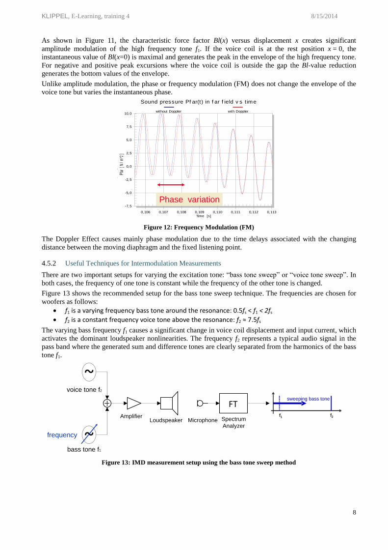
As shown in Figure 11, the characteristic force factor Bl(x) versus displacement x creates significant
amplitude modulation of the high frequency tone f1. If the voice coil is at the rest position x = 0, the
instantaneous value of Bl(x=0) is maximal and generates the peak in the envelope of the high frequency tone.
For negative and positive peak excursions where the voice coil is outside the gap the Bl-value reduction
generates the bottom values of the envelope.
Unlike amplitude modulation, the phase or frequency modulation (FM) does not change the envelope of the
voice tone but varies the instantaneous phase.
-7,5
-5,0
-2,5
0,0
2,5
5,0
7,5
10,0
0,106 0,107 0,108 0,109 0,110 0,111 0,112 0,113
Sound pressure Pf ar(t) in f ar f ield v s t ime
Pfar
[ N
/ m
^2 ]
Time [s]
without Doppler with Doppler
Phase variation
Figure 12: Frequency Modulation (FM)
The Doppler Effect causes mainly phase modulation due to the time delays associated with the changing
distance between the moving diaphragm and the fixed listening point.
4.5.2 Useful Techniques for Intermodulation Measurements
There are two important setups for varying the excitation tone: “bass tone sweep” or “voice tone sweep”. In
both cases, the frequency of one tone is constant while the frequency of the other tone is changed.
Figure 13 shows the recommended setup for the bass tone sweep technique. The frequencies are chosen for
woofers as follows:
f1 is a varying frequency bass tone around the resonance: 0.5fs < f1 < 2fs
f2 is a constant frequency voice tone above the resonance: f2 ≈ 7.5fs
The varying bass frequency f1 causes a significant change in voice coil displacement and input current, which
activates the dominant loudspeaker nonlinearities. The frequency f2 represents a typical audio signal in the
pass band where the generated sum and difference tones are clearly separated from the harmonics of the bass
tone f1.
bass tone f1
Loudspeaker
~
FT
Microphone Spectrum
Analyzer
Amplifier
~voice tone f2
frequency
f1 f2
sweeping bass tone
Figure 13: IMD measurement setup using the bass tone sweep method

KLIPPEL, E-Learning, training 4 8/15/2014
9
bass tone f1
Loudspeaker
~
FT
Microphone Spectrum
Analyzer
Amplifier
~voice tone f2
frequency
f1 f2
sweeping voice tone
Figure 14: IMD measurement setup using the voice tone sweep method
Figure 14 shows the recommended setup for the voice tone sweep technique. The frequencies are chosen for
woofers as follows:
f1 is a constant frequency bass tone below the resonance: f1 ≈ 0.5fs
f2 is a varying frequency voice tone over the audio band with 8fs < f2 < 20fs
The voice tone sweep method ensures an almost constant peak voice coil displacement while allowing
sufficient separation between the bass tone f1 harmonics and the voice tone f2 sum and difference tones. As
the voice tone is swept the total IMD measurement varies. Thus, the voice sweep method reveals the
frequency dependency of the intermodulation distortion on the frequency of the signal components in the
audio band.
4.6 Multi-tone Distortion Measurement
The multi-tone complex signal is comprised of a multitude of tones at known frequencies. During the
measurement, each tone generates harmonics. In addition, the tones interact providing a variety of difference
and summed tones similar to an actual audio music signal. For this reason, the multi-tone complex is used to
simulate the normal working conditions of a loudspeaker.
Signal source
Loudspeaker
~ FT
MicrophoneSpectrum
AnalyzerAmplifier
Filter
f
Sparse multi tone complex
f
Spectrum of distortion components
f
Figure 15: Multi-tone distortion measurement
When using the multi-tone complex signal, the nonlinear distortions are detected between the frequency
tones. Therefore, the multi-tone signal has a sparse spectrum. The ambient noise floor can be measured by
performing an additional measurement without any excitation signal. The bandwidth, shape and density of
the multi-tone complex signal can easily be adjusted to satisfy the target application of a particular transducer
or a complete loudspeaker system. It is important to note that the distortion spectrum resulting from this
measurement reveals no diagnostic information regarding the symmetrical and asymmetrical shapes of the
nonlinearities.

KLIPPEL, E-Learning, training 4 8/15/2014
10
4.7 Rub & Buzz Measurement
In order to easily separate the excitation tone from the generated impulsive distortion, a single tone or a
sinusoidal sweep is the preferred stimulus for exciting the distortions associated with irregular defects such
as voice coil rubbing, buzzing, loose particles, air leakage and hard limiting of the suspension or voice coil
former.
The distortions created by irregular defects are more impulsive than the nonlinear distortions generated by
the regular nonlinearities in the motor, suspension and diaphragm. In a conventional total harmonic distortion
(THD) measurement, the harmonic distortion generated by the regular nonlinearities are dominant. As a
result, the irregular distortions cannot be detected in the measurement. In addition, the distortion from
irregular defects may be audible even if the rms value of their higher order components (n > 20) are below
the noise level in a conventional THD measurement.
4.7.1 Impulsive and Higher-order Distortion
The irregular defects listed in 4.7 above generate distortion having a particular impulsive fine structure in the
time domain as shown in distortion signal d(t) in Figure 16. The impulsive behavior is evident in higher-
order harmonics and other signal components which are initiated and synchronized by the nonlinear defect.
Thus, both amplitude and phase information of the distortion signal provide valuable clues in determining
the source of the defect. Since the interpretation of a complex spectrum is difficult, it is more useful to
analyze the high-pass filtered time signal d(t) shown in Figure 16. Since irregular distortion is basically seen
in higher frequencies, the lower order distortion components are separated from the original microphone
signal by using a high-pass tracking filter.
At the output of the tracking filter some important measures are derived from the impulsive distortion signal
d(t):
- Peak value of higher-order distortion (PHD)
- RMS value of higher-order distortion (MHD)
- Crest factor of higher-order distortion (CHD)
- Instantaneous crest factor of higher-order distortion (ICHD)
sinusoidal
sweep
generator
Drive
Unit
~ tracking
filter
microphone
high-passcut-off frequency fc > 10f
instantaneous frequency f
Squarer + integrator
Peak
detector
electro-acoustical system
Ratio crest factor (CHD)
peak value(PHD)
rms value(MHD)
Total Sound Pressure Impulsive Distortion
So
un
d P
ress
ure
[m
Pa]
Time [ms]
RatioRectifier
InstantaneousCrest factor
(ICHD)
d(t)
d(t)
p(t)
p(t)
Figure 16: Measurement of defects by time domain analysis
4.7.2 Peak value of Impulsive Distortion
The most important characteristic of the impulsive distortion is the peak value (PHD). The rms-value (MHD)
corresponds with the power of the irregular distortion while the peak value is a more sensitive measurement
to show the impulsive symptoms in the fine structure of the waveform.
The PHD critical level is best evaluated relative to the loudspeakers passband sound pressure level.
Figure 17 shows the absolute PHD value exceeding a PHD limit set to 40 dB below the fundamental mean
sound pressure level in the passband. The frequency band between 40 and 70 Hz shows significant distortion.

KLIPPEL, E-Learning, training 4 8/15/2014
11
Figure 17: Absolut PHD (red thick line) and PHD limit (blue dashed line)
4.7.3 Crest Factor of Higher-order Distortion
The Crest factor of the Higher-order Distortion is a relative measure which describes the ratio between the
peak value and the rms value of the distortion within one period of the fundamental. This value describes the
impulsiveness of the distortion signal. A constant DC signal has a crest factor of 0 dB. A sinusoidal signal has
a crest factor of 3 dB. A distortion generated by regular nonlinearities or measurement noise usually reaches
a crest factor of 12 dB. Typical irregular distortions generated by loudspeaker defects can have crest factors
larger than 12 dB.
The Instantaneous Crest Higher-order Distortion (ICHD) describes the ratio between the absolute value
instantaneous distortion value |d(t)| and rms value MHD. This measure is useful for investigating the fine
structure of the impulsive distortion. When mapped to state variables, such as voice coil displacement or
sound pressure output, valuable information about the physical cause (bottoming, coil rubbing,
compression …) of the distortion can be determined.
Figure 18: Instantaneous crest factor of higher-order distortion (color) versus frequency and voice coil
displacement
Figure 18 shows the ICHD value as a function of the voice coil displacement (vertical axis) and the
instantaneous frequency, which is correlated with the sweep time of the logarithmic chirp used as the
stimulus. As shown in Figure 18, the black spots at negative excursions for the excitation frequencies
between 20 and 50 Hz indicating a bottoming of the voice coil former against the back plate.
-2,0
-1,5
-1,0
-0,5
0,0
0,5
1,0
1,5
2,0
2,5
20 100 200 500 1k 2k
Instantaneous crest harmonic distortion (ICHD)
Dis
pla
cem
ent
X
[mm
]
Frequency [Hz]
-29
-27
-25
-23
-21
-19
-17
-15
-13
-11
-9
-7
-5
-3
-1
1
3
5
7
9
11
13
0
20
40
60
80
100
120
10 20 50 100 200 500 1k 2k 5k 10k
Fundamental + Harmonic distortion components
Signal at IN1
dB
- [
V]
(rm
s)
Frequency [Hz]
Fundamental THD 2nd Harmonic 3rd Harmonic Absolute PHD Fund. mean (100 to 500 Hz) PHD limit (-40dB)
KLIPPEL, E-Learning, training 4 8/15/2014
12
5 Preparatory Questions
Check your theoretical knowledge before you start Section 6. Answer the questions by selecting all correct
responses (sometimes, there will be more than one).
QUESTION 1: Does the generation of the nonlinear distortion components depend on the frequency of the
excitation tone(s) in the stimulus?
□ MC a: Yes, the generation of the nonlinear distortions (harmonics, intermodulation and dc
components) depend on the frequency of the excitation tone because the loudspeaker is a
dynamic nonlinear system.
□ MC b: No, the generation of the nonlinear distortions (harmonics, intermodulation and dc
components …) are independent of the frequency of the excitation tone because the
loudspeaker is a static nonlinear system without any memory (like a diode with a nonlinear
transfer characteristic between input and output).
QUESTION 2: Does the generation of the nonlinear distortion components depend on the amplitude of the
excitation tone(s) in the stimulus?
□ MC a: No, the amplitude of the nonlinear distortion components generated in the output signal are
independent of the amplitude of the spectral components in the stimulus.
□ MC b: Yes, the amplitude of the nonlinear distortion components always increase when the
amplitude of the spectral components in the stimulus are increased.
□ MC c: Yes, the amplitude of the nonlinear distortion components may increase or decrease when
the amplitude of the spectral components in the stimulus are increased.
QUESTION 3: Do the loudspeaker nonlinearities affect the fundamental component?
□ MC a: No, the loudspeaker nonlinearities produce only harmonic distortions which are multiples
of the fundamental component. The amplitude and phase of the fundamental component in
the output signal can be calculated by multiplying the linear transfer function H(jω) with
the fundamental in the stimulus.
□ MC b: Yes, the fundamental component is also affected by the loudspeaker nonlinearities. In most
cases, the measured amplitude of the fundamental in the acoustic output of a nonlinear
loudspeaker is less than the predicted output using the linear transfer function. However, at
the resonance frequency, the nonlinear loudspeaker may produce more output of the
fundamental component due to the loss of electrical damping.
QUESTION 4: What does the measured DC component in the voice coil displacement reveal?
□ MC a: A DC component is generated by asymmetries in the nonlinear parameters (motor and
suspension nonlinearities) causing a partial rectification of the AC displacement. The sign
of the DC component (indicating voice coil movement towards or away from the back
plate) gives information about the orientation of the shape of the asymmetry.
□ MC b: A DC component may also be generated by loudspeaker instabilities even when the
loudspeaker nonlinearities are symmetrical.
□ MC c: A DC component in the voice coil displacement is a symptom of loudspeaker nonlinearities
but has no diagnostic value because a DC component is not audible.
QUESTION 5: Does the harmonic distortion measurement describe the nonlinear transfer behaviour of the
loudspeaker completely?
□ MC a: Yes, provided harmonic distortions are measured by using a sinusoidal sweep (chirp)
covering the complete audio band.
□ MC b: Yes, provided all orders of the harmonic distortion and the nonlinear compression of the
fundamental are measured as a function of the frequency and amplitude of the sinusoidal
stimulus.
□ MC c: No, because a single tone stimulus cannot generate intermodulation distortion. IMD
requires a stimulus comprised of more than one spectral component (two-tone).
KLIPPEL, E-Learning, training 4 8/15/2014
13
QUESTION 6: Does the frequency response of the absolute harmonic distortion have the same curve shape
as the relative harmonic distortion (as defined by IEC and other standards)?
□ MC a: Yes, the curve shapes are identical when the relative harmonic distortion is expressed in dB
(for example: -40 dB corresponds with 1 % distortion).
□ MC b: No, the relative harmonic distortion is the amplitude of the absolute distortion referred to
the amplitude of the total signal. Thus, the frequency response of the relative harmonic
distortion will have a different curve shape.
QUESTION 7: How do you detect rub & buzz and other irregular loudspeaker defects reliably?
□ MC a: The measurement of the 2nd
-order and 3rd
-order intermodulation components using a two-
tone stimulus is a reliable technique for measuring rub & buzz.
□ MC b: The measurement of the total harmonic distortion (THD) considers the amplitudes of all
harmonic components. The THD generated by rub & buzz and other irregular loudspeaker
defects is much less than the THD generated by the regular nonlinearities inherent in the
motor and suspension. As a result, to detect the unique symptoms of irregular defects, an
additional high-pass filter is required to suppress the low-order harmonic distortion
components generated by regular loudspeaker nonlinearities.
□ MC c: The irregular loudspeaker defects generate impulsive distortion components having a high
crest factor (high ratio of peak to rms value). Therefore, a time domain analysis is required
to consider the amplitude and phase of the distortion components at high frequencies.
□ MC d: A multi-tone distortion measurement is a reliable technique for detecting rub &buzz
provided the stimulus is comprised of a sufficient number of tones logarithmically
distributed over the audio band.
6 Interpretation of Distortion Measurements (no hardware required)
Step 1: View the demo movie Loudspeaker Distortion Measurements located at www.klippel.de/training to
see how practical distortion measurements are performed.
Step 2: Run the Software dB-Lab and open the file Loudspeaker Distortion Measurements.kdbx
Advice: Before submitting your answers, it is recommended to do the following exercises offline!
6.1 Harmonic Distortion Measurement
6.1.1 2nd
- and 3rd
- Order Distortion
Step 3: Open the operation 1a TRF SPL Fund + Harm 1.5V, which shows a transient measurement of
the harmonic distortion of the transducer by using a sinusoidal sweep where the instantaneous
frequency increases logarithmically over time. In the result window “Fundamental + Harmonics”
compare the curves 2nd
Harmonic with the Total Harmonic Distortion (THD).
QUESTION 8: In which frequency range is the absolute 2nd
-order distortion component dominating the
THD?
□ MC a: Below 40 Hz
□ MC b: 40 < f < 250 Hz
□ MC c: For all frequencies above 250 Hz
QUESTION 9: In which frequency range is the absolute 3rd
-order distortion component dominating the
THD?
□ MC a: Below 40 Hz
□ MC b: 40 < f < 250 Hz
□ MC c: For all frequencies above 250 Hz
KLIPPEL, E-Learning, training 4 8/15/2014
14
Step 4: In the same operation 1a TRF SPL Fund + Harm 1.5V look at the result window
“Y1 (f) Spectrum” and compare the Signal lines (blue), which is the reproduced stimulus, with the
Noise floor, found in the microphone signal with muted stimulus (black).
QUESTION 10: Is the measurement of 2nd
- and 3rd
-order harmonic distortion for excitation frequencies
between 40 and 250 Hz corrupted by steady-state noise (e.g. generated by air
conditioning)?
□ MC a: No, the measurement is not corrupted by steady-state noise because the signal to noise ratio
(SNR) is greater than 40 dB in the frequency range 80 Hz < f < 750 Hz where the 2nd
- and
3rd
- order harmonic distortions are being measured.
□ MC b: Yes, the signal to noise ratio (SNR) is about 40 dB at 40 Hz which is not sufficient for
measuring the harmonics at 40 Hz.
Step 5: Open the operation 1b TRF SPL Fund + Harm 6V, which shows the harmonic distortion of the
same transducer using the same measurement setup but at a much higher sinusoidal stimulus
voltage (6 V instead of 1.5 V). In the result window “Fundamental + Harmonics” observe the 3rd
Harmonic and answer the following question:
QUESTION 11: What is the physical reason for the absolute level of the total harmonic distortion to be
decreasing at frequencies above resonance (fs < f < 4fs)?
□ MC a: The sound pressure output is almost constant in this frequency range.
□ MC b: The electrical input current increases from resonance (120 Hz) to the minimum of the
electrical impedance curve (450 Hz).
□ MC c: The displacement decreases above the resonance frequency by 12 dB per octave.
6.1.2 Displacement
Step 6: Open the operation 2a TRF X Fund + Harm 6V and inspect the frequency range from 150 Hz
to 1.5 kHz in the result windows “Fundamental + Harmonics”, “Harmonic Distortion (relative)”
and “Y2 (f) Spectrum”.
QUESTION 12: What causes the increase of the relative total harmonic distortion, shown as curve THD in
X, in result window “Harmonic distortion (relative)” in this frequency range?
□ MC a: The harmonic distortion measurement is corrupted by measurement noise. As shown in the
result window “Y2 (f) Spectrum” of the displacement, the measured voice coil
displacement disappears into the noise floor at 1 kHz. The resulting low signal-to-noise
ratio (SNR) causes an almost constant value of absolute distortion (-50 dB) in this
frequency range. The relative distortion, which is the ratio between absolute distortion and
total displacement, increases because the total displacement decreases by 40 dB.
□ MC b: The loudspeaker generates more distortion at higher frequencies.
□ MC c: The laser sensor is limiting and generates this distortion.
Step 7: In the same operation 2a TRF X Fund + Harm 6V open the result window
“Harmonic Distortion (relative)”. Compare the curve THD in X, representing the relative THD
found in the displacement signal, with the curve THD in SPL, representing the relative THD found
in the sound pressure signal (this curve has been copied from result window
“Harmonic Distortion (relative)” in the operation 1b TRF SPL Fund + Harm 6V.
QUESTION 13: Why is the relative THD measured in sound pressure higher than the relative THD
measured in displacement at low frequencies (f < 150 Hz)?
□ MC a: The radiation and propagation of the sound is highly nonlinear and increases the distortion
at low frequencies.
□ MC b: The amplitudes of both relative measurements depend on the frequency response of the
fundamental component. Below resonance, the fundamental of the SPL measurement
decreases but the fundamental of the displacement measurement is almost constant.
□ MC c: The noise generated by the microphone increases the THD in the acoustical measurement.
KLIPPEL, E-Learning, training 4 8/15/2014
15
Step 8: Open the operation 2b DIS X Fund., DC, Short and inspect the result window
“DC Component” which shows displacement versus frequency.
QUESTION 14: Is the DC Component independent of the frequency of the sinusoidal stimulus?
□ MC a: No, the direction of the DC Component depends not only on the frequency but also on the
shape of the nonlinearity. In this case the DC Component is maximal at the resonance
frequency.
□ MC b: No, the direction of the DC Component depends not only on the frequency but also on the
shape of the nonlinearity. In this case the DC Component is maximal at frequencies below
50 Hz and above 300 Hz.
□ MC c: Yes. The DC Component is always maximal at low frequencies, where there is more
displacement.
Step 9: Open the operation 2c DIS X Motor stability and inspect the result window “DC Component”
which shows displacement versus voltage.
QUESTION 15: How does the dc displacement vary versus voltage?
□ MC a: The DC displacement becomes less at higher voltages because the progressive suspension
produces a symmetrical increase in the stiffness at positive and negative displacements,
which improves the stability of the loudspeaker.
□ MC b: The DC displacement is relatively small at low voltages but increases rapidly at critically
higher voltages. This behaviour reveals instability of the electro-dynamic motor.
□ MC c: The DC displacement increases slowly with rising voltage. This behaviour is typical for a
loudspeaker which is stable but has significant asymmetries in the nonlinear parameters.
6.1.3 Equivalent Input Distortion
Step 10: Select the operation 3a TRF SPL EHID 6 V. Open the property page Processing and ensure
that the checkboxes Curve and Level in section Reference are disabled. Open the result window
“Fundamental + Harmonics”. Copy the curve Fundamental onto the clipboard and paste it into
the EDIT button found in section Reference on the property page Processing. The imported curve
is used for inverse filtering of the microphone signal. The response of the fundamental component
should now become almost flat. By doing this, the nonlinear distortion at the sensor (e.g.
microphone) has been transformed to the input of the loudspeaker (e.g. electrical terminals).
QUESTION 16: Why is the calculation of the equivalent input distortion useful?
□ MC a: The dominant nonlinear distortions generated by motor and suspension nonlinearities are
generated in the one-dimensional signal domain close to the electrical input. These
nonlinearities produce the same amount of equivalent harmonic input distortion (EHID) as
measured by the microphone (independent of the microphone position). If the EHID
measurement shows a dependency on the microphone position, the nonlinearities are
located in the multi-dimensional signal path (e.g. cone vibration or sound radiation).
□ MC b: The amplitude response of the microphone has no influence on the Equivalent Harmonic
Input Distortion (EHID) measurement because the inverse filtering removes the linear
properties of the fundamental and the linear properties of the microphone.
□ MC c: The influence of room reflections and room modes are removed from the Equivalent Input
Distortion (EHID) measurement because linear sound propagation can be compensated by
inverse filtering the fundamental component.
Step 11: Open the result window “Harmonic Distortion (relative)” in the Operation 3b X EHID 6 V
which shows curves 2nd
EHID X and 3rd
EIHID X of the laser measurement. Compare these curves
with the curves 2nd
EHID SPL and 3rd
EHID SPL that have been copied from corresponding result
window of the microphone measurement 3a TRF SPL EHID 6 V.
KLIPPEL, E-Learning, training 4 8/15/2014
16
QUESTION 17: Are the relative Equivalent Harmonic Input Distortions (EHID’s) derived from the
microphone and the laser measurement similar at all frequencies?
□ MC a: No, at low frequencies (f < 100 Hz), the laser and microphone measurement give almost
the same EHID. However, at high frequencies (f > 150 Hz), the EHID calculated from the
laser is corrupted by measurement noise resulting in insufficient SNR.
□ MC b: Yes, the laser and the microphone measurement give almost the same EHID at any
frequency.
6.2 Intermodulation Distortion Measurement
6.2.1 Intermodulation Distortion
Step 12: Open the operation 4a DIS SPL IMD (bass sweep) and view the frequency response of the
intermodulation distortion in the result windows “2nd
Intermod, %” and “3rd
Intermod, %”.
QUESTION 18: At which frequency of the bass tone are the relative intermodulation distortions (in percent)
maximal?
□ MC a: At 35 Hz.
□ MC b: At 95 Hz (close to the resonance frequency).
□ MC c: At 235 Hz.
Step 13: In the same operation 4a DIS SPL IMD (bass sweep) view the result window
“Fundamental Component” to compare the 6.00V curve with the Fundamental X 6V and the
Fundamental I 6V curves, imported from the operations 4b DIS X (bass sweep) and
4c DIS current (bass sweep), respectively.
QUESTION 19: Which state variable has the largest magnitude when the generation of intermodulation
distortion increases in the frequency range 20 Hz < f < 120 Hz?
□ MC a: Displacement
□ MC b: Current
□ MC c: Sound Pressure
6.2.2 AM / FM Distortion
Step 14: Open the operation 4d DIS SPL IMD (voice sweep) and inspect the result window
“Waveform Y1” showing the sound pressure signal for a two-tone signal comprised of a first voice
tone f1 = 1.9 kHz and a second bass tone f2 = 23 Hz.
QUESTION 20: What does the sound pressure time signal reveal?
□ MC a: The envelope of the voice tone at 1.9 kHz varies over time. The distance between the
maxima is about 43 ms which corresponds with the period of the bass tone at 23 Hz.
□ MC b: The phase of the voice tone varies over time.
Step 15: Open result window “Modulation” in the same operation 4d DIS SPL IMD (voice sweep) and
compare the curve AM distortion(Lamd), representing pure Amplitude Modulation (AM) distortion,
with the total intermodulation distortion Ldm (cumul), which considers both Amplitude and
Frequency Modulation (AM + FM).
QUESTION 21: What causes the variations in the voice tone envelope at 1.9 kHz?
□ MC a: Amplitude Modulation (AM) because the value of AM distortion(Lamd) is close to the
value of the total intermodulation distortion Ldm (cumul).
□ MC b: Frequency Modulation (FM) because the value of AM distortion(Lamd) is much less than
the value of the total intermodulation distortion Ldm (cumul).
KLIPPEL, E-Learning, training 4 8/15/2014
17
6.2.3 Distortion in the Input Current
Step 16: Open the operation 5a TRF CURRENT Harm 6 V and in the result window
“Fundamental + Harmonics” view the absolute 2nd
Harmonic and 3rd
Harmonic Distortion in the
input current versus frequency.
QUESTION 22: How does the 2nd
-order harmonic distortion in the input current change over the frequency
range from 200 Hz to 1.75 kHz?
□ MC a: The absolute value of the harmonic distortion in the input current is constant.
□ MC b: The absolute value of the harmonic distortion in the input current decreases approximately
5 dB per octave.
□ MC c: The absolute value of the harmonic distortion in the input current decreases approximately
12 dB per octave.
Step 17: In the same operation 5a TRF CURRENT Harm 6 V and the same result window
“Fundamental + Harmonics” view the frequency response of the fundamental component of the
current in the frequency range from 200 Hz to 1.75 kHz. Copy the corresponding curves of the
sound pressure in 1b TRF SPL Fund-Harm 6 V and displacement in
2a TRF X Fund + Harm 6 V and paste them into this window and compare the curves.
QUESTION 23: Which state variable of the loudspeaker decreases in this frequency range? Hint: it may
activate a loudspeaker nonlinearity that generates distortion in the input current between
200 Hz and 1.75 kHz?
□ MC a: Voice coil displacement is decreasing by approximately 12 dB/octave.
□ MC b: Current is slightly decreasing due to the effect of the voice coil inductance.
Step 18: Open the result window “3rd
Intermod, %” located in the operation
5b DIS CURRENT IMD (bass sweep) and compare the 6V curve, representing the 3rd
-order
intermodulation distortion in the input current, with the IMD SPL 6V curve, corresponding with the
3rd
-order intermodulation found in the sound pressure copied from the operation
4a DIS SPL IMD (bass sweep).
QUESTION 24: Does the 3rd
order intermodulation distortion in current and sound pressure have a common
cause (the same loudspeaker nonlinearity)?
□ MC a: No, because the 3rd
-order IMD in the sound pressure is much larger in amplitude than the
3rd
-order IMD in the current signal. Thus, the source of the distortion is in the mechanical
or acoustical domains.
□ MC b: Yes, because the values are similar. Thus, the source of the distortion is in the electrical
domain.
Step 19: Open the operation 5c DIS CURRENT IMD (voice sweep) and view the result windows
“2nd
Intermod %” and “3rd
Intermod %”. Compare the 3V intermodulation curve, found in the
electrical input current, with the IMD SPL 3V curve, found in the sound pressure output copied
from the corresponding result windows in operation 4d DIS SPL IMD (voice sweep). Note:
both 2nd
-order and 3rd
-order intermodulation distortions have a local maximum (exceeding 30 %) at
1.9 kHz.
QUESTION 25: Where is the nonlinearity which causes the high intermodulation at 1.9 kHz located?
□ MC a: The nonlinearity is located in the electrical domain because the intermodulation distortions
found in the input current are similar to the IMD found in the sound pressure output.
□ MC b: The nonlinearity is located in the mechanical or acoustical domain because the IMD found
in the electrical input current is much less than the IMD found in the sound pressure.
KLIPPEL, E-Learning, training 4 8/15/2014
18
6.3 Multi-tone Distortion Measurement
Step 20: Open the operation 6a LPM MTD 1/10th oct and inspect the result window “P(f) Spectrum”.
Compare the two curves Noise Floor and Noise+Distortion.
QUESTION 26: Is the distortion-to-noise ratio sufficient to separate the nonlinear distortion components
from steady-state ambient noise?
□ MC a: No, the noise floor curve is similar to the Noise+Distortion curve.
□ MC b: Yes, the noise floor curve is 30 dB below the Noise+Distortion curve.
Step 21: In the same operation 6a LPM MTD 1/10th oct and the same result window “P(f) Spectrum”
compare the Noise+Distortion spectrum with the corresponding spectrum in the result window
“Current (f) Spectrum”.
QUESTION 27: Use the cross cursor to read the approximate level difference between the fundamental
component and the distortion peak value at 2 kHz. Where is the dominant cause of the
distortion located?
□ MC a: It is located in the electrical domain because the input current shows dominant distortion
(the same level difference exists between distortion and fundamental in both the input
current and the sound pressure output).
□ MC b: It is located in the mechanical or acoustical domain because the input current shows less
distortion (a level difference of 30 dB exists between distortion and fundamental in the
input current, which is much higher than the corresponding difference of 15 dB in the
sound pressure output).
Step 22: Select the operation 6b LPM MTD 1/10th oct hp which shows the multi-tone distortion
measurement where the frequency components below 300 Hz are attenuated using a high-pass
filtered stimulus. In the result window “P(f) Spectrum”, compare the signal line (high-pass) curve
with the signal line (full band) curve that was copied from the corresponding result window in the
operation 6a LPM MTD 1/10th oct. Open the result window “Multi-tone distortion” and
compare the MTD high pass curve with the MTD full band curve. Note: the distortions are
significantly reduced (20 dB) when the high-pass filtered stimulus is used.
QUESTION 28: Which state signal, that has a significant influence on the generation of MTD above
300 Hz, is significantly reduced by applying a high-pass filter?
□ MC a: voice coil displacement
□ MC b: electrical input current
□ MC c: terminal voltage
□ MC d: sound pressure output at microphone
6.4 Rub & Buzz Measurement
Step 23: Select the Operation 7c TRF peak harmonics 8V and open the result window
“Fundamental+Harmonics”. Activate the cross cursor and view the difference in the magnitude
between the THD curve, representing the absolute total harmonic distortion at 70 Hz, and the
magnitude of the 21st harmonic component at 70 Hz.
Comment: If the 21st-order harmonic is not displayed press “c” or right click in the graph area and
select customize. Select property page Subset, press Ctrl on the keyboard and select curve 21th.
KLIPPEL, E-Learning, training 4 8/15/2014
19
QUESTION 29: Is the measurement of the 21st-order harmonic component a reliable way for detecting
rub & buzz and other irregular defects?
□ MC a: Yes, because the regular nonlinearities inherent in the motor and suspension do not
generate significant contributions to higher-order harmonics.
□ MC b: No, a higher-order harmonic component (n > 10) has low spectral energy and is located
close to the noise floor. Only significant defects can be detected by reading a higher order
single harmonic. Sensitive measurement techniques in the time domain and spectral
information between the harmonic components in the frequency domain are required to
determine the amplitude and phase information of multiple harmonics (10 < n < 300).
Step 24: Open the result window “Instantaneous Distortion” in the same operation
7c TRF peak harmonics 8V and view the peak value of the high-pass filtered PHD with n > 10.
This window shows the Distortion curve and the Distortion 1V curve that was copied from
operation 7a TRF peak harmonics 1V using a lower input terminal voltage.
Step 25: Open the result window “Fundamental+Harmonics” in the same operation
7c TRF peak harmonics 8V and view the Absolute PHD curve. Search for the frequency range
where the Absolute PHD exceeds the permissible PHD limit curve which is 40 dB lower than the
mean value of the fundamental component.
Step 26: Select the Operation 7d TRF Crest harmonics 8V and inspect the result window
“Instantaneous Distortion”. Search for the frequency range where the instantaneous crest factor
ICHD exceeds the permissible limit Thresh curve, which has been set to 12 dB.
QUESTION 30: Do the peak value PHD and crest factor ICHD exceed the corresponding limits at the same
frequency?
□ MC a: Yes, a loudspeaker irregular defect that has both a high PHD and a high ICHD value in the
frequency range from 40 to 60 Hz indicates the generation of impulsive distortion.
□ MC b: No, the instantaneous crest factor ICHD exceeds the limit value in the frequency range 40
to 60 Hz but the PHD is more than 40 dB below the fundamental. Although the impulsive
properties of the distortion indicate an irregular defect, the small peak value shows that the
defect is negligible.
□ MC c: No, although the peak value PHD exceeds the permissible limit, the low instantaneous crest
factor ICHD indicates that the distortions are not impulsive. The peak value may be caused
by measurement noise and is not critical.
Step 27: View the result window “Instantaneous Distortion 3D” in the same operation
7d TRF Crest harmonics 8V and search for the conditions (frequency, displacement) where the
instantaneous crest factor ICHD exceeds the 12 dB threshold corresponding with “black spots” in
the diagram.
QUESTION 31: Determine the voice coil displacement where the impulsive distortion occurs and the crest
factor exceeds the 12 dB threshold.
□ MC a: In the frequency range 35 < f < 65 Hz the impulsive distortion occurs at the positive peak
of the displacement (at 3 mm peak).
□ MC b: In the frequency range 35 < f < 65 Hz the impulsive distortion occurs at the negative peak
of the displacement (at 3 mm peak).
□ MC c: In the frequency range 35 < f < 65 Hz the impulsive distortion occurs at the negative peak
of the displacement (at 1 mm peak).
Step 28: View the result window “Modelled and Measured Response” in the same operation
7d TRF Crest harmonics 8V which shows the distortion waveform plotted as the Residual
curve versus instantaneous frequency. Zoom into the Residual curve at 60 Hz to see the impulsive
distortion generated at the maximum negative sound pressure signal which corresponds to a
positive displacement maximum (sound pressure is proportional to acceleration).
KLIPPEL, E-Learning, training 4 8/15/2014
20
7 Performing Measurements (Hardware required)
7.1 Setup the Hardware
Default routing
Alternative routingLaser Head
ANR Laser Head
MIC
AMP
Main Power Supply
ANR Controller
Controller
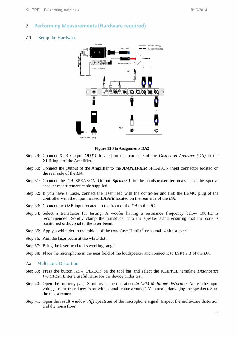
Figure 13 Pin Assignments DA2
Step 29: Connect XLR Output OUT 1 located on the rear side of the Distortion Analyzer (DA) to the
XLR Input of the Amplifier.
Step 30: Connect the Output of the Amplifier to the AMPLIFIER SPEAKON input connector located on
the rear side of the DA.
Step 31: Connect the DA SPEAKON Output Speaker 1 to the loudspeaker terminals. Use the special
speaker measurement cable supplied.
Step 32: If you have a Laser, connect the laser head with the controller and link the LEMO plug of the
controller with the input marked LASER located on the rear side of the DA.
Step 33: Connect the USB input located on the front of the DA to the PC.
Step 34: Select a transducer for testing. A woofer having a resonance frequency below 100 Hz is
recommended. Solidly clamp the transducer into the speaker stand ensuring that the cone is
positioned orthogonal to the laser beam.
Step 35: Apply a white dot to the middle of the cone (use TippEx® or a small white sticker).
Step 36: Aim the laser beam at the white dot.
Step 37: Bring the laser head to its working range.
Step 38: Place the microphone in the near field of the loudspeaker and connect it to INPUT 1 of the DA.
7.2 Multi-tone Distortion
Step 39: Press the button NEW OBJECT on the tool bar and select the KLIPPEL template Diagnostics
WOOFER. Enter a useful name for the device under test.
Step 40: Open the property page Stimulus in the operation 4g LPM Multitone distortion. Adjust the input
voltage to the transducer (start with a small value around 1 V to avoid damaging the speaker). Start
the measurement.
Step 41: Open the result window P(f) Spectrum of the microphone signal. Inspect the multi-tone distortion
and the noise floor.

KLIPPEL, E-Learning, training 4 8/15/2014
21
Step 42: Open the result window Multitone Distortion and read the maximum of the distortion. If the
distortion maximum is below -20 dB (less than 10 %), increase the voltage in the property page
Stimulus and repeat the measurement.
Step 43: For future measurements, make note of the final voltage determined in step 42.
Step 44: Open the result window X(t) and read the peak value of the displacement.
Step 45: Open the result window Current (f) spectrum. Determine the relative level of the distortion in the
current by finding the level difference between the multi-tone distortion maximum and the
fundamental in the current signal. Compare this result with the relative level of the distortion in the
sound pressure output. Is the dominant nonlinearity in the electrical domain?
7.3 Voice Coil Displacement
Step 46: Open the property page Stimulus for the operation 3a DIS X Fundamental DC and enter the voltage
used in the 4g LPM Multitone distortion for U end (use 0.1 V for U start). Start the measurement.
Step 47: Determine the peak and bottom value of the displacement in the result window PEAK + BOTTOM.
Step 48: In result window COMPRESSION, inspect the amplitude compression at frequencies below
resonance.
Step 49: Inspect the DC-displacement generated by the woofer. Find the frequency where the transducer
generates the largest DC-displacement and compare it with the transducer resonance frequency fs,
as shown in the result window Table Linear Parameters for the operation 4g LPM Multitone
distortion.
Step 50: Open the property page Stimulus for the operation 3b DIS motor stability and enter the critical
frequency f = 1.5 fs. Ensure that the voice coil temperature monitoring is enabled in property page
Protection and set the maximal allowed temperature increase to 60 K. Start the measurement. (The
protection based on temperature monitoring makes it possible to use a maximal voltage U end
which is higher than the voltage used in operation 4g LPM Multitone distortion.)
Step 51: Read the maximal value in the result window DC component and compare it with the AC
component shown in result window Fundamental Component. Is the motor stable?
7.4 Harmonic Distortion
Step 52: Open the property page Stimulus for the operation 4a TRF SPL + harmonics and adjust the
stimulus voltage to the value used in 4g LPM Multitone distortion. Ensure that the check box
“noise floor monitoring” is enabled. Start the measurement.
Step 53: Open the result window Y1(f) Spectrum and check the signal to noise ratio. Do you have an SNR
better than 30 dB in the frequency range of interest?
Step 54: Open the result window Impulse response and set the left and right window cursors around the
direct sound so that room reflections arriving at a later time will be suppressed.
Step 55: Inspect the harmonics in the result window Fundamental + Harmonics. Determine which order of
harmonic distortion dominates the total harmonic distortion (THD).
Step 56: Open the result window Harmonic Distortion and search for the frequency of maximum distortion
above fs. Compare the harmonic distortion at this frequency with the multi-tone distortion at the
same frequency in operation 4g LPM Multitone distortion. Explain the difference.
KLIPPEL, E-Learning, training 4 8/15/2014
22
7.5 Equivalent Input Distortion
Step 57: Copy the operation 4a TRF SPL + harmonics and paste it under the same object in dB-lab. Rename
the operation 4a TRF Equivalent Harmonics. Open the result window Fundamental + Harmonics
and copy the Fundamental curve onto the clipboard. Open the property page Processing and paste
this curve into the IMPORT button.
Step 58: View the window Fundamental + Harmonics and check that the Fundamental curve has become
almost flat and located close to zero. The harmonic distortion curves now shown in this window
represent the equivalent input distortion. Why are the EID’s almost constant for frequencies below
resonance?
Step 59: Open the result window Harmonic Distortion and compare the EID relative distortion with the
relative distortion found in the sound pressure output in the corresponding window of operation 4a
TRF SPL + harmonics.
7.6 Intermodulation Distortion
Step 60: Open the property page Stimulus of the operation 4e DIS IM Dist. (voice sweep) and enter the
voltage used in the 4g LPM Multitone distortion for U end (use 0.1 V for U start). Start the
measurement. Listen for fluctuation and roughness in the reproduced high frequency tone.
Step 61: View the result windows 2nd
Intermod, % and 3rd
Intermod, % and search for the frequency of
maximum intermodulation distortion fmax. Compare this value with the harmonic distortion at the
same frequency fmax in operation 4a TRF SPL + harmonics.
7.7 Rub&Buzz and other Irregular Distortion
Step 62: Open the property page Stimulus of the operation 5 TRF Rub and Buzz and enter the voltage value
1 V. Rename the measurement 5 TRF Rub and Buzz 1V. Start the measurement. Listen for
bottoming, voice coil rubbing and other symptoms of irregular defects.
Step 63: Open the result window Fundamental + Harmonics and search for the maximum in the Absolute
PHD curve. Does the curve exceed the PHD limit (-40 dB) curve? Repeat the measurement to
ensure that this maximum is reproducible and not caused by ambient noise. A loudspeaker without
any defect should produce only noise (a flat line which is independent of frequency).
Step 64: Hold an obstacle (pen, screw driver) at a close distance from the cone and start the measurement
again. If the cone has struck the obstacle and produced an impulse you will see a distinct increase
in the Absolute PHD. Open the property page I-Dist and select ICHD located under Measure. Open
the result window Instantaneous Distortion 3D showing the instantaneous crest factor versus
displacement and frequency. Find the positive displacement and frequency required for the cone’s
surface to hit the obstacle.
Step 65: Duplicate the measurement 5 TRF Rub and Buzz 1V and enter the voltage used in the 4g LPM
Multitone distortion. Rename the operation 5 TRF Rub and Buzz high voltage. Start the
measurement. Listen for bottoming, voice coil rubbing and other symptoms of irregular defects.
Open the result window Fundamental + Harmonics and search for the maximum in the Absolute
PHD curve. Repeat the measurement to ensure that this maximum is reproducible and not caused
by ambient noise. Does the curve exceed the PHD limit (-40 dB) curve? If not, increase the voltage
and start the measurement again.
Step 66: Open the result window Instantaneous Distortion 3D of the measurement 5 TRF Rub and Buzz
high voltage showing the instantaneous crest factor versus displacement and frequency. Search for
black spots in the 3D window and read the position of the voice coil where the impulsive distortion
is generated.
Step 67: Discuss the possible cause which could lead to the measured impulsive distortion.

KLIPPEL, E-Learning, training 4 8/15/2014
23
8 Further Literature
User Manual for the KLIPPEL R&D SYSTEM – Transfer Function (TRF)
User Manual for the KLIPPEL R&D SYSTEM – 3D Distortion Measurement (DIS)
User Manual for the KLIPPEL R&D SYSTEM – Linear Parameter Measurement (LPM)
Paper “Measurement of Equivalent Input Distortion”:
http://www.klippel.de/uploads/media/Measurement_of_Equivalent_Input_Distortion_03.pdf
Paper “Measurement of Impulsive Distortion, Rub and Buzz and other Disturbances”:
http://www.klippel.de/uploads/media/Measurement_of_Rub_and_Buzz_03.pdf