Lot sizing and scheduling - Survey and extensions - …homes.ieu.edu.tr/~aornek/ISE421_drexl_kimms.pdf · ELSEVIER European Journal of Operational Research 99 (1997) 221-235 EUROPEAN

E L S E V I E R European Journal of Operational Research 99 (1997) 221-235

EUROPEAN JOURNAL

OF OPERATIONAL RESEARCH

Invited Review

Lot sizing and scheduling - Survey and extensions A. Drexl *, A. K imms 1

Lehrstuhl fiir Produktion und Logistik, lnstitut fiir Betriebswirtschaflslehre, Christian-Albrechts-Universitdt zu Kiel, Olshausenstrafle 40, D-24118 Kiel, Germany

Received 3 December 1996

Abstract

This contribution summarizes recent work in the field of lot sizing and scheduling. The objective is not to give a compre- hensive literature survey, but to explain differences of formal models and to provide some first readings recommendations. Our focus is on capacitated, dynamic, and deterministic cases. To underscore the importance of the research efforts, current practice is described and its shortcomings are exposed. Mathematical programming models where the planning horizon is subdivided into several discrete periods are given for both approaches that are well-established and approaches which may represent tomorrow's state of the art. Two research directions are discussed in more detail: continuous time models and multi-level lot sizing and scheduling. The paper concludes with some advice for future research activities. (~) 1997 Elsevier Science B.V.

Keywords: Production planning; Lot sizing; Scheduling; Capacitated lot sizing problem; Discrete lot sizing and scheduling problem; Continuous setup lot sizing problem; Proportional lot sizing and scheduling problem; Batching and scheduling problem

1. Background and motivation

1.1. Prob l em context

Consider the organization of an in-house production system. Typically, the architecture of such a system is buil t up from several production cells, so-called seg- ments, which may be implemented in different fash- ions (flow lines or work centers for instance). This macro-structure further refines into a micro-structure as each segment provides the capabil i ty to perform a bunch o f operations.

Raw materials and component parts are floating concurrently through this complex system in order

* Corresponding author. Tel.: +49 431 880 1531, fax: +49 431 880 1531, e-mail: [email protected]

1 e-mail: [email protected]

to be processed and assembled until a final product comes out ready for deliverance.

Production planning and scheduling is one of the most challenging subjects for the management there. It appears to be an hierarchical process ranging from long- to medium- to short-term decisions. Our focus will be the short-term scope which links to medium- term decisions via the master product ion schedule (MPS) . The MPS defines the external (or indepen- dent) demand, i.e. due dates and order sizes for final products. The goal now is to find a feasible product ion plan which meets the requests and provides release dates and amounts for all products including component parts. For economical reasons, finding a feasible plan is not sufficient. In the usual case, product ion plans can be evaluated by means of an object ive function (e.g. a function which measures the setup and the holding costs) . Then, the aim is to find a feasible

0377-2217/97/$17.00 (~) 1997 Elsevier Science B.V. All rights reserved. PII S0377-22 17 (97)00030-1

222 A. Drexl, A. Kimms/European Journal of Operational Research 99 (1997) 221-235

production plan with optimum (or close to optimum) objective function value.

1.2. Problem outline

Let the manufacturing process be triggered by orders which originate from customers or from other fa- cilities. Suppose now that the output of the make-to- order system under concern is or at least includes a set of non-customized products. Certainly, this is a valid assumption for many firms no matter what industry they belong to and no matter what size they are.

To motivate a planning activity, we first need to identify a subject of concern that is worth (in terms of economical rationale) considering. A first clue are large inventories. Due to the opportunity costs of capi- tal and the direct costs of storing goods, holding items in inventory and thus causing holding costs should be avoided. On the other hand, if different parts are mak- ing use of common resources, say machines, and a setup action must take place to prepare proper operation, then opportunity costs (i.e. setup costs) are incurred since production is delayed. Another aspect of sharing resources is that the production of such parts cannot coincide if different setup states are required. Hence, orders must be sequenced. In summary, we have a trade-off between low setup costs (favoring large production lots) and low holding costs (favoring a lot-for-lot-like production where sequence decisions have to be made due to sharing common resources). Essentially, the problem of short-term production planning turns out to be a lot sizing and scheduling problem, then.

If we ask about how to solve this production planning problem, we first need a deeper understanding of its basic attributes. The first key element we have to remember is the stream of component parts floating through a complex production system. Operations may be executed only if parts which are subject of these particular operations are indeed available. In other words, a production plan must respect the precedence rela- tions of operations. Hence, multi-level structures must be taken into account. For the sake of convenience, we do not further distinguish between operations and items (also called products or parts). Each operation produces an item, and each item is the output of an operation. Apparently, we face a multi-item problem here.

The second key element of our problem is the presence of scarce capacity. As usual in in-house production systems, producing an item requires a certain amount of one or more resources (e.g. manpower, machine time, energy, etc.) with limited capacity per time unit. Thus, production planning must take scarce capacity into account.

The (known or estimated) external demand (given by the MPS) is to be met promptly at the end of each period. Backlogging and shortages are not allowed here, which enforces a high service level. The demand may vary over time. This is called dynamic demand. All relevant data for the planning process are assumed to be deterministic, which is justified by having a short-term planning problem on hand.

1.3. Case descriptions

To underscore the practical importance of (multi- level) lot sizing and scheduling, we enumerate some real-world reports demanding for methods to be applied. A case at Eastman Kodak Company and an elaborate analysis attached with results of a simula- tion of this case can be found in [67]. Another case at Owens-Corning Fiberglas Corporation is described in [89]. Mathematical models of cases can be found in [48] (tire production) and [ 111 ] (pharmaceutical industry).

1.4. Current practice

In most commercial production planning and control systems, the logic of manufacturing resource planning (MRP II) is implemented [ 117]. The working principle of this approach tries to construct feasible production plans in a stepwise manner. Basically, three phases can be discriminated, which are outlined below.

Phase I: Starting with end items, lot sizes are computed level by level for all items in the multi-level gozinto structure. By doing so, capacity constraints are ignored. Phase II: The result obtained by phase I usually ex- ceeds the available capacity in some periods. Hence, some lots are shifted in order to find a plan which meets the capacity limits. By doing so, precedence re- lations among the items are ignored.

A. Drexl, A. Kimms/European Journal of Operational Research 99 (1997) 221-235

Phase III: Sequence decisions are made and orders are released to the shop floor.

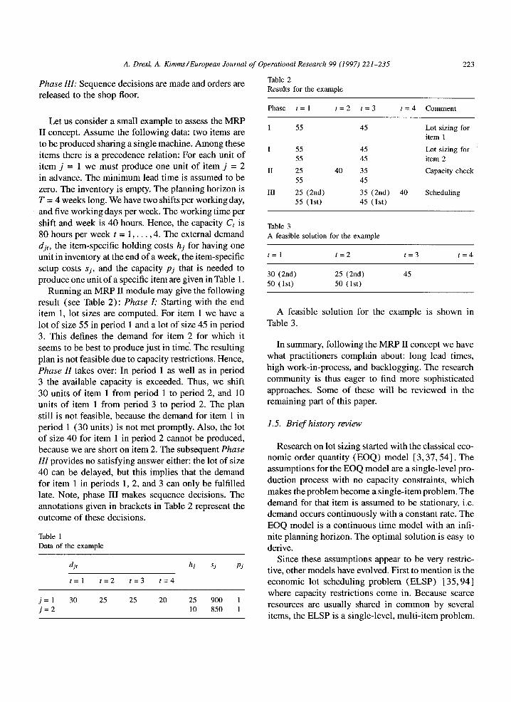
Let us consider a small example to assess the MRP II concept. Assume the following data: two items are to be produced sharing a single machine. Among these items there is a precedence relation: For each unit o f item j = 1 we must produce one unit of item j = 2 in advance. The minimum lead time is assumed to be zero. The inventory is empty. The planning horizon is T = 4 weeks long. We have two shifts per working day, and five working days per week. The working time per shift and week is 40 hours. Hence, the capacity Ct is 80 hours per week t = 1 . . . . . 4. The external demand d jr, the item-specific holding costs hj for having one unit in inventory at the end of a week, the item-specific setup costs s j , and the capacity pj that is needed to produce one unit o f a specific item are given in Table 1.

Running an MRP II module may give the following result (see Table 2): Phase I: Starting with the end item 1, lot sizes are computed. For item 1 we have a lot of size 55 in period 1 and a lot of size 45 in period 3. This defines the demand for item 2 for which it seems to be best to produce just in time'. The resulting plan is not feasible due to capacity restrictions. Hence, Phase H takes over: In period 1 as well as in period 3 the available capacity is exceeded. Thus, we shift 30 units of item 1 from period 1 to period 2, and 10 units of item 1 from period 3 to period 2. The plan still is not feasible, because the demand for item 1 in period 1 (30 units) is not met promptly. Also, the lot of size 40 for item 1 in period 2 cannot be produced, because we are short on item 2. The subsequent Phase III provides no satisfying answer either: the lot of size 40 can be delayed, but this implies that the demand for item 1 in periods 1, 2, and 3 can only be fulfilled late. Note, phase III makes sequence decisions. The annotations given in brackets in Table 2 represent the outcome of these decisions.

Table 1 Data of the example

d.# hj sj pj

t = l t=2 t = 3 t = 4

j = 1 30 25 25 20 25 900 1 j = 2 10 850 1

Table 2 Results for the example

223

Table 3 A feasible solution for the example

t = l t = 2 t=3 t = 4

30 (2nd) 25 (2nd) 45 50 (lst) 50 (lst)

A feasible solution for the example is shown in Table 3.

In summary, following the MRP II concept we have what practitioners complain about: long lead times, high work-in-process, and backlogging. The research community is thus eager to find more sophisticated approaches. Some of these will be reviewed in the remaining part of this paper.

1.5. Br ie f history review

Research on lot sizing started with the classical economic order quantity (EOQ) model [3, 37, 54]. The assumptions for the EOQ model are a single-level production process with no capacity constraints, which makes the problem become a single-item problem. The demand for that item is assumed to be stationary, i.e. demand occurs continuously with a constant rate. The EOQ model is a continuous time model with an infinite planning horizon. The optimal solution is easy to derive.

Since these assumptions appear to be very restrictive, other models have evolved. First to mention is the economic lot scheduling problem (ELSP) [35, 94] where capacity restrictions come in. Because scarce resources are usually shared in common by several items, the ELSP is a single-level, multi-item problem.

Phase t = 1 t = 2 t = 3 t = 4 Comment

I 55 45 Lot sizing for item 1

I 55 45 Lot sizing for 55 45 item 2

II 25 40 35 Capacity check 55 45

III 25 (2nd) 35 (2nd) 40 Scheduling 55 (lst) 45 (lst)

224 A. DrexL A. Kimms/European Journal of Operational Research 99 (1997) 221-235

However, the ELSP still assumes stationary demand. Table 5 Parameters for the CLSP

It is a continuous time model, too, and the planning horizon is infinite again. Solving the ELSP optimally is NP-hard [ 60]. Hence, heuristics dominate the arena [31,46, 118].

A quite different step was made from the EOQ model assumptions towards dynamic demand conditions. The so-called Wagner-Whitin (WW) problem [ 114] assumes a finite planning horizon which is subdivided into several discrete periods. Demand is given per period and may vary over time. However, capacity limits are not considered which means that the single- level WW problem is a single-item problem. The problem can be viewed as a shortest path problem. This interpretation reveals that optimal solution procedures for the WW problem exist which are polynomially bounded. Exact solution procedures are presented in [1], [38] and [113].

The next generation of models has combined capacitated and dynamic approaches and bothered the community since then. Surveys of lot sizing literature can be found in [6], [26] and [79].

Also, scheduling was integrated with lot size decisions. This is what our review is about. Section 2 thus presents established single-level models for lot sizing and scheduling as well as new trends. Section 3 discusses continuous time approaches. Multi-level extensions are dealt with in Section 4. Finally, Section 5 provides some suggestions for future research directions.

2. Single-level lot sizing and scheduling

2.1. The capac i ta ted lot s iz ing p ro b l em

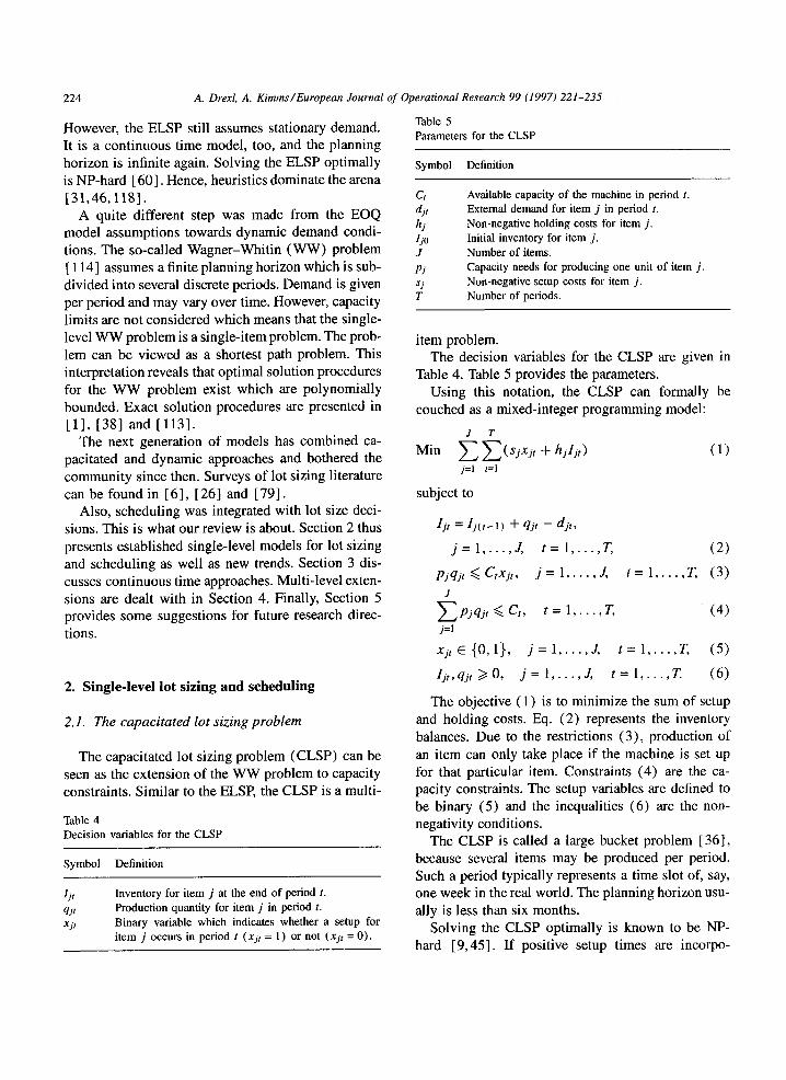
The capacitated lot sizing problem (CLSP) can be seen as the extension of the WW problem to capacity constraints. Similar to the ELSP, the CLSP is a multi-

Table 4 Decision variables for the CLSP

Symbol Definition

jr

q jr xjt

Inventory for item j at the end of period t. Production quantity for item j in period t. Binary variable which indicates whether a setup for item j occurs in period t (xjt = 1) or not (x j t = 0) .

Symbol Definition

Ct ~lj, hj #o J pj sj T

Available capacity of the machine in period t. External demand for item j in period t. Non-negative holding costs for item j . Initial inventory for item j . Number of items. Capacity needs for producing one unit of item j . Non-negative setup costs for item j . Number of periods.

item problem. The decision variables for the CLSP are given in

Table 4. Table 5 provides the parameters. Using this notation, the CLSP can formally be

couched as a mixed-integer programming model:

J T

M i n Z ~ ( s j x j , ~- h j l j t ) (1) j=l t=l

subject to

I j t = l j(t-l) + qjt -- djt ,

j = l . . . . . J, t = l . . . . . T, (2)

Pjqj t <~ Ctxjt, J = I . . . . . J, t = 1 . . . . . T, (3) J

Pj qjt <~ Ct, t = 1 . . . . . T, (4 ) j=l

x j t E { 0 , 1 } , j = l . . . . . J, t = l . . . . . T, (5)

I j t , q j t>~O, j = l . . . . . J, t = l . . . . . T. (6)

The objective ( 1 ) is to minimize the sum of setup and holding costs. Eq. (2) represents the inventory balances. Due to the restrictions (3), production of an item can only take place if the machine is set up for that particular item. Constraints (4) are the capacity constraints. The setup variables are defined to be binary (5) and the inequalities (6) are the non- negativity conditions.

The CLSP is called a large bucket problem [36], because several items may be produced per period. Such a period typically represents a time slot of, say, one week in the real world. The planning horizon usually is less than six months.

Solving the CLSP optimally is known to be NP- hard [9,45]. If positive setup times are incorpo-

A. DrexL A. Kimms /European Journal

rated into the model, the feasibility problem is NP- complete [82]. Hence, there are only a few attempts to solve the CLSP optimally [7,21,36,47]. Many authors have developed heuristics [ 16, 28, 29, 57, 76, 83].

Scheduling decisions are, however, not integrated into the CLSP. The usual approach therefore is to solve the CLSP first, and to solve a scheduling problem for each period separately afterwards. A review of the scheduling literature can be found in [ 10], [ 11 ] and [90]. A recent attempt to hierarchically integrate lot sizing and scheduling is described in [24], [25] and [80].

Let us return to the example given in Section 1.4. If we would use a solution procedure for the CLSP dur- ing phase I, the problem of capacity violations would vanish and phase II would no longer be necessary. However, due to the multi-level gozinto structure it is easy to figure out an example where the CLSP is used on a level by level basis and does not yield a feasible solution. Also, phase III, which is the scheduling phase, is not integrated.

2.2. The discrete lot s iz ing and schedul ing prob lem

Subdividing the (macro-)periods of the CLSP into several (micro-) periods leads to the discrete lot sizing and scheduling problem (DLSP). In this subsection we will use the term period for short in order to re- fer to a micro-period. The fundamental assumption of the DLSP is the so-called 'all-or-nothing' production: Only one item may be produced per period, and, if so, production uses the full capacity.

The DLSP is called a small bucket problem [36], because at most one item can be produced per period. Hence, periods in the DLSP model usually correspond to small time slots such as hours or shifts.

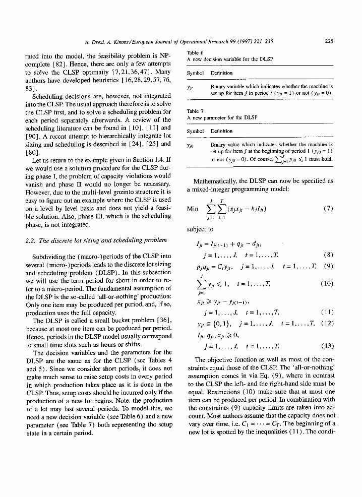
The decision variables and the parameters for the DLSP are the same as for the CLSP (see Tables 4 and 5). Since we consider short periods, it does not make much sense to raise setup costs in every period in which production takes place as it is done in the CLSP. Thus, setup costs should be incurred only if the production of a new lot begins. Note, the production of a lot may last several periods. To model this, we need a new decision variable (see Table 6) and a new parameter (see Table 7) both representing the setup state in a certain period.

of Operational Research 99 (1997) 221-235

Table 6 A new decision variable for the DLSP

225

Symbol Definition

Yjt Binary variable which indicates whether the machine is set up for item j in period t (Yjt = 1) or not (Yjt = 0).

Table 7 A new parameter for the DLSP

Symbol Definition

Yjo Binary value which indicates whether the machine is set up for item j at the beginning of period 1 (Yjo = 1 )

J or not (YjO = 0). Of course, E j = I YjO ~ 1 must hold.

Mathematically, the DLSP can now be specified as a mixed-integer programming model:

J T

M i n E E ( s j x j t "[-hj l j t ) (7) j=l t=l

subject to

ljt = l j ( t -1) + qjt -- dj, ,

j = l . . . . . J, t = l . . . . . T, (8)

pjq j t = C t Y j t , J = 1 . . . . . J, t = 1 . . . . . T, (9)

J

E Y j t <<. 1, t = 1 . . . . . T, (10) j=l

Xjt • Yjt -- Yj(t--l) ,

j = l . . . . . J, t = l . . . . . T, (11)

y j t E { O , 1) , j = l . . . . . J, t = l . . . . . T, (12)

I jr, qjt, Xjt ~ O,

j = l . . . . . J, t = l . . . . . T. (13)

The objective function as well as most of the constraints equal those of the CLSP. The 'all-or-nothing' assumption comes in via Eq. (9), where in contrast to the CLSP the left- and the right-hand side must be equal. Restrictions (10) make sure that at most one item can be produced per period. In combination with the constraints (9) capacity limits are taken into account. Most authors assume that the capacity does not vary over time, i.e. Cl . . . . . CT. T h e beginning of a new lot is spotted by the inequalities ( 11 ). The condi-


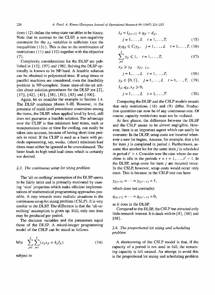
tions (12) define the setup state variables to be binary. Note that in contrast to the CLSP, a non-negativity constraint for the xjt variables is sufficient (see the inequalities (13)) . This is due to the combination of restrictions ( 11 ) and (12) together with the objective (7).

Complexity considerations for the DLSP are published in [ 12], [97] and [98]. Solving the DLSP optimally is known to be NP-hard. A feasible solution can be obtained in polynomial time. If setup times or parallel machines are considered, even the feasibility problem is NP-complete. Some state-of-the-art arti- cles about solution procedures for the DLSP are [2], [17], [42], [43], [58], [81], [85] and [100].

Again, let us consider the example in Section 1.4. The DLSP combines phases I-III . However, in the presence of multi-level precedence constraints among the items, the DLSP, when applied level by level, still does not guarantee a feasible solution. The advantage over the CLSP is that minimum lead times, such as transportation time or time for cooling, can easily be taken into account, because of having short time periods in mind. I f the CLSP is used as a basis with periods representing, say, weeks, (short) minimum lead times must either be ignored or be overestimated. The latter leads to high total lead times which is certainly not desired.

2.3. The continuous setup lot sizing problem

The 'all-or-nothing' assumption of the DLSP seems to be fairly strict and is primarily motivated by causing 'nice' properties which make efficient implemen- tations of mathematical programming approaches pos- sible. A step towards more realistic situations is the continuous setup lot sizing problem (CSLP). It is very similar to the DLSP. The difference is that the 'all-or- nothing' assumption is given up. Still, only one item may be produced per period.

The decision variables and the parameters equal those of the DLSP. A mixed-integer programming model of the CSLP can be stated as follows:

J T

Min Z ~--~(SjXjt "~ hjI j t ) (14) j=l t=l

subject to

I j t = Ij(t--1) -~- qjt -- dj t ,

j = l . . . . . J, t = l . . . . . T, (15)

Pjqjt <~ CtYjt, j = l . . . . . J, t = l . . . . . T , ( 1 6 )

J

Z Y j t <~ l , t = l . . . . . T, (17) j=l

Xjt ~ Yjt -- Y j ( t -1 ) ,

j = l . . . . . J, t = l . . . . . T, (18)

y j t C { O , 1}, j = l . . . . . J, t = l . . . . . T, (19)

I jr, q jr, x jr >1 O,

j = l . . . . . J, t = l . . . . . T. (20)

Comparing the DLSP and the CSLP models reveals that only restrictions (16) and (9) differ. Produc- tion quantities can now be of any continuous size. Of course, capacity restrictions must not be violated.

At first glance, the difference between the DLSP and the CSLP seems to be almost negligible. How- ever, there is an important aspect which can easily be overseen: In the DLSP, setup costs are incurred when- ever a new lot begins. Assume, for example, that a lot for item j is completed in period t. Furthermore, assume that another lot for the same item j is scheduled in period t ~ > t. Consider now the case where the machine is idle in the periods 7- = t + 1 . . . . . t ~ - 1. In the DLSP, setup costs for item j are incurred twice. In the CSLP, however, setup costs would occur only once. This is because in the CSLP one can have

Yj(t+l) = " " " = Yj(F--1) = 1,

which does not contradict

qj(t+l) . . . . . qj(F--1) = 0 ,

as it does in the DLSE Compared to the DLSP, the CSLP has attracted only

little research interest. It is dealt with in [ 8], [ 66] and [68].

2.4. The proportional lot sizing and scheduling problem

A shortcoming of the CSLP model is that, if the capacity of a period is not used in full, the remaining capacity is left unused. An attempt to avoid this is the proportional lot sizing and scheduling problem

A. Drexl, A. Kimms/European Journal of Operational Research 99 (1997) 221-235 227

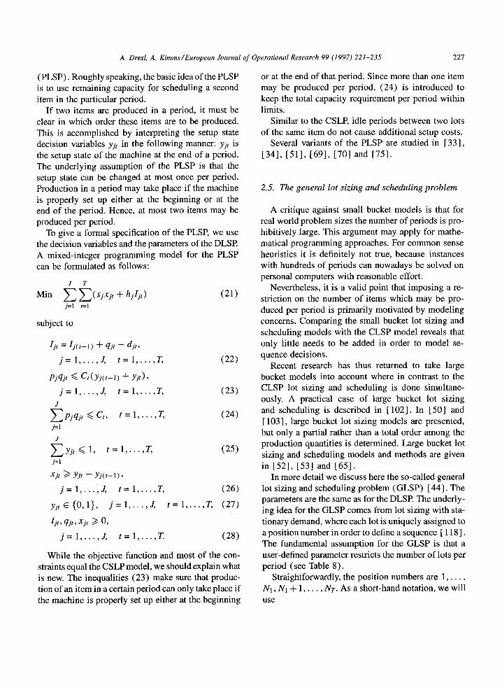
(PLSP). Roughly speaking, the basic idea of the PLSP is to use remaining capacity for scheduling a second item in the particular period.

If two items are produced in a period, it must be clear in which order these items are to be produced. This is accomplished by interpreting the setup state decision variables Yjt in the following manner: Yjt is the setup state of the machine at the end of a period. The underlying assumption of the PLSP is that the setup state can be changed at most once per period. Production in a period may take place if the machine is properly set up either at the beginning or at the end of the period. Hence, at most two items may be produced per period.

To give a formal specification of the PLSP, we use the decision variables and the parameters of the DLSP. A mixed-integer programming model for the PLSP can be formulated as follows:

J T

Min ~_ ,~ '~ ( s j x j t "}-hjljt) (21) j=l t=l

subject to

Ij t m l j ( t_ l ) Jr qjt -- djt,

j = l . . . . . J, t = l . . . . . T, (22)

Pjqjt ~ Ct (Y j ( t -1) ~- Yj t ) ,

j = l . . . . . J, t = l . . . . . T, (23)

J

~ P j q j t <<, Ct, t = 1 . . . . . T, (24) j=l

J

Z Y j t ~ 1, t = 1 . . . . . T, (25) j=l

xjt >~ Yjt - Yj(t-1),

j = l . . . . . J, t = l . . . . . T, (26)

y j t E { O , 1}, j = l . . . . . J, t = l . . . . . T, (27)

lit, q jr, X jr >1 O,

j = l . . . . . J, t = l . . . . . T. (28)

While the objective function and most of the constraints equal the CSLP model, we should explain what is new. The inequalities (23) make sure that production of an item in a certain period can only take place if the machine is properly set up either at the beginning

or at the end of that period. Since more than one item may be produced per period, (24) is introduced to keep the total capacity requirement per period within limits.

Similar to the CSLP, idle periods between two lots of the same item do not cause additional setup costs.

Several variants of the PLSP are studied in [33], [34], [51], [69], [70] and [75].

2.5. The general lot sizing and scheduling problem

A critique against small bucket models is that for real world problem sizes the number of periods is pro- hibitively large. This argument may apply for mathematical programming approaches. For common sense heuristics it is definitely not true, because instances with hundreds of periods can nowadays be solved on personal computers with reasonable effort.

Nevertheless, it is a valid point that imposing a restriction on the number of items which may be produced per period is primarily motivated by modeling concerns. Comparing the small bucket lot sizing and scheduling models with the CLSP model reveals that only little needs to be added in order to model sequence decisions.

Recent research has thus returned to take large bucket models into account where in contrast to the CLSP lot sizing and scheduling is done simultane- ously. A practical case of large bucket lot sizing and scheduling is described in [102]. In [50] and [ 103], large bucket lot sizing models are presented, but only a partial rather than a total order among the production quantities is determined. Large bucket lot sizing and scheduling models and methods are given in [52], [53] and [65].

In more detail we discuss here the so-called general lot sizing and scheduling problem (GLSP) [44]. The parameters are the same as for the DLSP. The underlying idea for the GLSP comes from lot sizing with stationary demand, where each lot is uniquely assigned to a position number in order to define a sequence [ 118 ]. The fundamental assumption for the GLSP is that a user-defined parameter restricts the number of lots per period (see Table 8).

Straightforwardly, the position numbers are 1 . . . . . N1, Nl + 1 . . . . . Nr. As a short-hand notation, we will u s e

228 A. DrexL A. Kimms/European Journal of Operational Research 99 (1997) 221-235

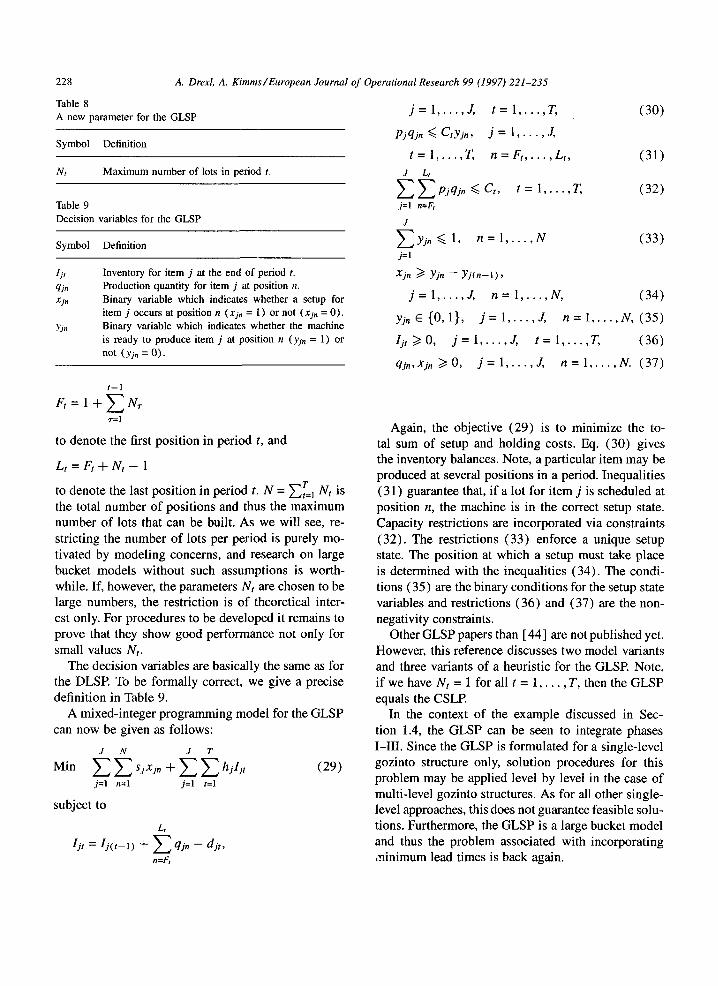
Table 8 A new parameter for the GLSP

Symbol Definition

Nt Maximum number of lots in period t.

Table 9 Decision variables for the GLSP

Symbol Definition

lit qjn Xjn

Y j,,

Inventory for item j at the end of period t. Production quantity for item j at position n. Binary variable which indicates whether a setup for item j occurs at position n (Xjn = 1) or not (Xjn = 0) . Binary variable which indicates whether the machine is ready to produce item j at position n (Yjn = 1) or not (Yjn = 0).

t--1

Ft= I + ~-~ N~ 7"=1

to denote the first position in period t, and

Lt = Ft + Nt - 1

to denote the last position in period t. N = ~--]t~l Nt is the total number of positions and thus the maximum number of lots that can be built. As we will see, re- stricting the number of lots per period is purely motivated by modeling concerns, and research on large bucket models without such assumptions is worth- while. If, however, the parameters Nt are chosen to be large numbers, the restriction is of theoretical interest only. For procedures to be developed it remains to prove that they show good performance not only for small values Nt.

The decision variables are basically the same as for the DLSP. To be formally correct, we give a precise definition in Table 9.

A mixed-integer programming model for the GLSP can now be given as follows:

J N J T

Min Z Z s . i X j n - k - Z Z h j l j t (29) j=l n=l j=l t=l

subject to

Lt

Ijt = I j ( t -1) + ~-~ qjn -- ajt, n=Ft

j = l . . . . . J, t = l . . . . . T, (30)

Pjqjn ~ CtYjn, J = 1 . . . . . J,

t = l . . . . . T, n = F t . . . . . Lt, (31) J L,

Z Z p j q j n <~ Ct, t = I . . . . . T, ( 3 2 )

j=l n=Ft

J

Z y j n <<. 1, n= l . . . . . N (33) j=l

Xjn ) Yjn -- Y j (n - l ) ,

j = l . . . . . J, n = l . . . . . N, (34)

y j n E { O , 1}, j = l . . . . . J, n = l . . . . . N , ( 3 5 )

l j ,~>0, j = l . . . . . J, t = l . . . . . T, (36)

qjn,Xjn>~O, j = l . . . . . J, n = l . . . . . N. (37)

Again, the objective (29) is to minimize the total sum of setup and holding costs. Eq. (30) gives the inventory balances. Note, a particular item may be produced at several positions in a period. Inequalities (31 ) guarantee that, if a lot for item j is scheduled at position n, the machine is in the correct setup state. Capacity restrictions are incorporated via constraints (32). The restrictions (33) enforce a unique setup state. The position at which a setup must take place is determined with the inequalities (34). The conditions (35) are the binary conditions for the setup state variables and restrictions (36) and (37) are the non- negativity constraints.

Other GLSP papers than [44] are not published yet. However, this reference discusses two model variants and three variants of a heuristic for the GLSP. Note, if we have Nt = 1 for all t = 1 . . . . . T, then the GLSP equals the CSLE

In the context of the example discussed in Sec- tion 1.4, the GLSP can be seen to integrate phases I-III . Since the GLSP is formulated for a single-level gozinto structure only, solution procedures for this problem may be applied level by level in the case of multi-level gozinto structures. As for all other single- level approaches, this does not guarantee feasible solutions. Furthermore, the GLSP is a large bucket model and thus the problem associated with incorporating minimum lead times is back again.


3. Continuous time lot sizing and scheduling Table 11 Parameters for the BSP

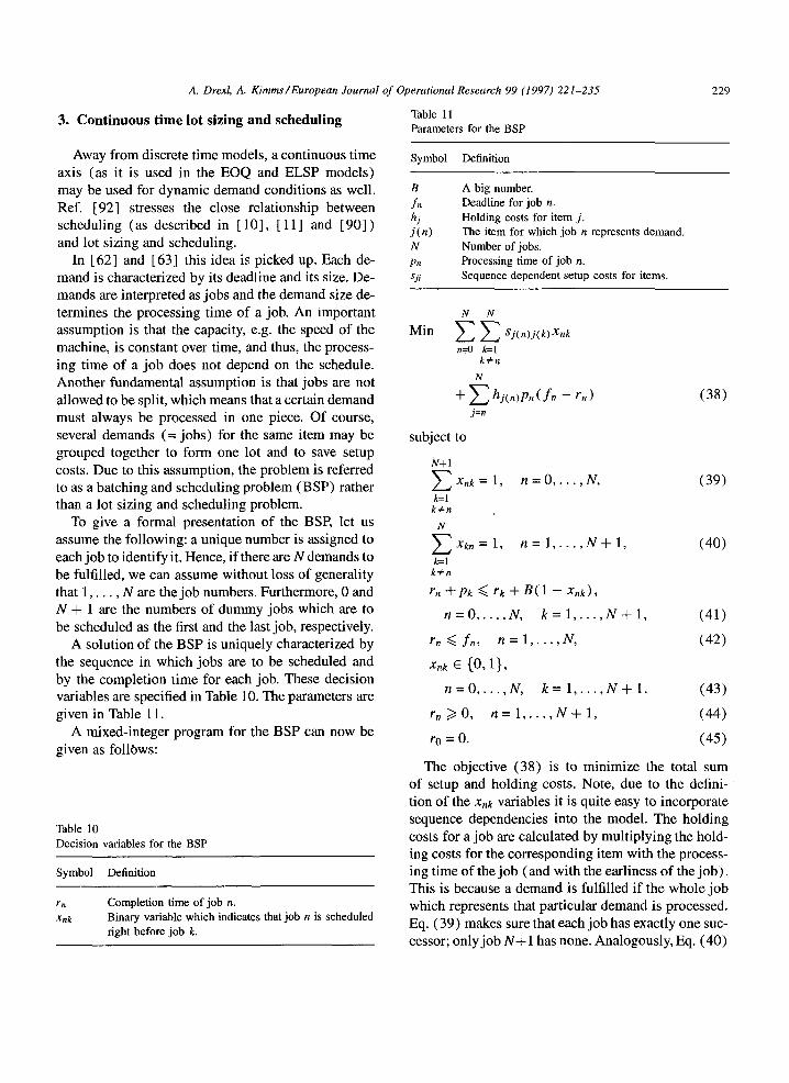
Away from discrete time models, a continuous time axis (as it is used in the EOQ and ELSP models) may be used for dynamic demand conditions as well. Ref. [92] stresses the close relationship between scheduling (as described in [ 10], [ 11] and [90]) and lot sizing and scheduling.

In [62] and [63] this idea is picked up. Each demand is characterized by its deadline and its size. De- mands are interpreted as jobs and the demand size de- termines the processing time of a job. An important assumption is that the capacity, e.g. the speed of the machine, is constant over time, and thus, the processing time of a job does not depend on the schedule. Another fundamental assumption is that jobs are not allowed to be split, which means that a certain demand must always be processed in one piece. Of course, several demands (= jobs) for the same item may be grouped together to form one lot and to save setup costs. Due to this assumption, the problem is referred to as a batching and scheduling problem (BSP) rather than a lot sizing and scheduling problem.

To give a formal presentation of the BSP, let us assume the following: a unique number is assigned to each job to identify it. Hence, if there are N demands to be fulfilled, we can assume without loss of generality that 1 . . . . . N are the job numbers. Furthermore, 0 and N + 1 are the numbers of dummy jobs which are to be scheduled as the first and the last job, respectively.

A solution of the BSP is uniquely characterized by the sequence in which jobs are to be scheduled and by the completion time for each job. These decision variables are specified in Table 10. The parameters are given in Table 11.

A mixed-integer program for the BSP can now be given as follows:

Table 10 Decision variables for the BSP

Symbol Definition

rn Completion time of job n. xnk Binary variable which indicates that job n is scheduled

right before job k.

Symbol Definition

B

fn hj j(n) N Pn sji

A big number. Deadline for job n. Holding costs for item j . The item for which job n represents demand. Number of jobs. Processing time of job n. Sequence dependent setup costs for items.

N N

Min ~ ~ Sj(n)j(k)Xnk n--0 k=l

kq:n

N

+ ~ hj(n)Pn(fn - rn) (38) j=n

subject to

N+I

Z x " k = l ' n = 0 . . . . . N, (39) k=l kg~n

N

~-~Xtn=l , n = l . . . . . N + I , (40) k=l

kg:n

rn +Pt <~ rk + B(1- - Xnk),

n = 0 . . . . . N, k = l . . . . . N + l , (41)

rn <~ fn, n= l . . . . . N, (42)

x.~ ~ {o, 1},

n = 0 . . . . . N, k = l . . . . . N + I , (43)

rn>/O, n = l . . . . . N + I , (44)

ro =0 . (45)

The objective (38) is to minimize the total sum of setup and holding costs. Note, due to the definition of the Xnk variables it is quite easy to incorporate sequence dependencies into the model. The holding costs for a job are calculated by multiplying the holding costs for the corresponding item with the processing time of the job (and with the earliness of the job). This is because a demand is fulfilled if the whole job which represents that particular demand is processed. Eq. (39) makes sure that each job has exactly one successor; only job N + 1 has none. Analogously, Eq. (40)


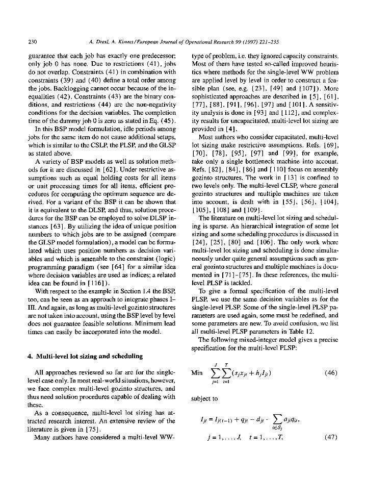
guarantee that each job has exactly one predecessor; only job 0 has none. Due to restrictions (41), jobs do not overlap. Constraints (41) in combination with constraints (39) and (40) define a total order among the jobs. Backlogging cannot occur because of the inequalities (42). Constraints (43) are the binary conditions, and restrictions (44) are the non-negativity conditions for the decision variables. The completion time of the dummy job 0 is zero as stated in Eq. (45).

In this BSP model formulation, idle periods among jobs for the same item do not cause additional setups, which is similar to the CSLP, the PLSP, and the GLSP as stated above.

A variety of BSP models as well as solution methods for it are discussed in [62]. Under restrictive assumptions such as equal holding costs for all items or unit processing times for all items, efficient procedures for computing the optimum sequence are de- rived. For a variant of the BSP it can be shown that it is equivalent to the DLSP, and thus, solution procedures for the BSP can be employed to solve DLSP instances [ 63 ]. By utilizing the idea of unique position numbers to which jobs are to be assigned (compare the GLSP model formulation), a model can be formulated which uses position numbers as decision variables and which is amenable to the constraint (logic) programming paradigm (see [64] for a similar idea where decision variables are used as indices; a related idea can be found in [ 116] ).

With respect to the example in Section 1.4 the BSP, too, can be seen as an approach to integrate phases I - III. And again, as long as multi-level gozinto structures are not taken into account, using the BSP level by level does not guarantee feasible solutions. Minimum lead times can easily be incorporated into the model.

4. Multi-level lot sizing and scheduling

All approaches reviewed so far are for the single- level case only. In most real-world situations, however, we face complex multi-level gozinto structures, and thus need solution procedures capable of dealing with these.

As a consequence, multi-level lot sizing has attracted research interest. An extensive review of the literature is given in [75].

Many authors have considered a multi-level WW-

type of problem, i.e. they ignored capacity constraints. Most of them have tested so-called improved heuristics where methods for the single-level WW problem are applied level by level in order to construct a feasible plan (see, e.g. [23], [49] and [107]). More sophisticated approaches are described in [ 5 ], [ 61 ], [77], [88], [91], [96], [97] and [101]. A sensitiv- ity analysis is done in [93] and [ 112], and complexity results for uncapacitated, multi-level lot sizing are provided in [4].

Most authors who consider capacitated, multi-level lot sizing make restrictive assumptions. Refs. [69], [70], [78], [95], [97] and [99], for example, take only a single bottleneck machine into account. Refs. [82], [84], [86] and [110] focus on assembly gozinto structures. The work in [ 13] is confined to two levels only. The multi-level CLSP, where general gozinto structures and multiple machines are taken into account, is dealt with in [55], [56], [104], [ 105], [ 108] and [ 109].

The literature on multi-level lot sizing and scheduling is sparse. An hierarchical integration of some lot sizing and some scheduling procedures is discussed in [24], [25], [80] and [106]. The only work where multi-level lot sizing and scheduling is done simulta- neously under quite general assumptions such as general gozinto structures and multiple machines is docu- mented in [71 ] - [75] . In these references, the multi- level PLSP is tackled.

To give a formal specification of the multi-level PLSP, we use the same decision variables as for the single-level PLSP. Some of the single-level PLSP parameters are used again, some must be redefined, and some parameters are new. To avoid confusion, we list all multi-level PLSP parameters in Table 12.

The following mixed-integer model gives a precise specification for the multi-level PLSP:

J T

Min EE(sjxj, +hjljt) (46) j=l t=l

subject to

I j t = I j ( t - l ) -+- qjt -- djt - E ajiqit, iESj

j = l . . . . . J, t = l . . . . . T, (47)


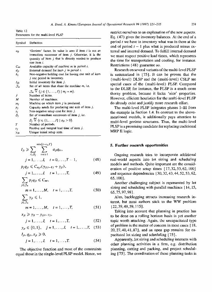
Table 12 Parameters for the multi-level PLSP

Symbol Definition

Cmt d j, hj

ljo ,7,,

J M mj Pj s: s:

T vj Yjo

'Gozinto' factor. Its value is zero if item i is not an immediate successor of item j . Otherwise, it is the quantity of item j that is directly needed to produce one item i. Available capacity of machine m in period t. External demand for item j in period t. Non-negative holding cost for having one unit of item j one period in inventory. Initial inventory for item j . Set of all items that share the machine m, i.e.

Jm de__f {j 6 {1 . . . . . J} I mj = m}.

Number of items. Number of machines. Machine on which item j is produced. Capacity needs for producing one unit of item j . Non-negative setup cost for item j . Set of immediate successors of item j , i.e.

Sj de__f{/ C {1 . . . . . J} [aji > 0}.

Number of periods. Positive and integral lead time of item j . Unique initial setup state.

restrict ourselves to an explanation of the new aspects. Eq. (47) gives the inventory balances. At the end of a period t we have in inventory what was in there at the end of period t - 1 plus what is produced minus external and internal demand. To fulfill internal demand we must respect positive lead times, which represents the time for transportation and cooling, for instance. Restrictions (48) guarantee so.

Research on several variants of the multi-level PLSP is summarized in [75]. It can be proven that the (multi-level) DLSP and the (multi-level) CSLP are special cases of the (multi-level) PLSE Compared to the DLSP, for instance, the PLSP is a much more thorny problem, because it lacks 'nice' properties. However, efficient heuristics for the multi-level PLSP do already exist and justify more research effort.

The multi-level PLSP integrates phases I-III from the example in Section 1.4. In contrast to the above- mentioned models, it additionally pays attention to multi-level gozinto structures. Thus, the multi-level PLSP is a promising candidate for replacing traditional MRP II logic.

nfin{ t+vj,T }

iGSj r=t+l

j = l . . . . . J, t = 0 . . . . . T - 1, (48)

pjqjt ~ Cm:(yj<t-l) + Yjt),

j = l . . . . . J, t = l . . . . . T, (49)

Z PJ q jr <<. Cmt, jcJ , ,

m = l . . . . . M, t = l . . . . . T, (50)

jeff , ,

m = l . . . . . M, t = l . . . . . T, (51)

Xjt ) Yjt -- Yj( t - - l ) ,

j = l . . . . . J, t = l . . . . . T, (52)

yjt E {O, 1}, j = l . . . . . J, t = l . . . . . T, (53)

]jt, qjt,Xjt >1 O,

j = l . . . . . J, t = l . . . . . T. (54)

The objective function and most of the constraints equal those in the single-level PLSP model. Hence, we

5. Further research opportunit ies

Ongoing research tries to incorporate additional real-world aspects into lot sizing and scheduling models and methods. Quite important are the consid- eration of positive setup times [ 17, 32, 53, 62, 100] and sequence dependencies [30, 32, 43, 44, 52, 53, 62, 6 5 , 1 0 0 ] .

Another challenging subject is represented by lot sizing and scheduling with parallel machines [ 14, 15, 65, 75, 97, 98].

Also, backlogging attracts increasing research interest, but most authors stick to the WW problem [22,39,49,59, 115].

Taking into account that planning in practice has to be done on a rolling horizon basis is yet another topic worth attacking. Again, the uncapacitated type of problem is the matter of concern in most cases [ 18, 20,27,40,41,87], and an open gap remains for capacitated lot sizing and scheduling [ 75 ].

Apparently, lot sizing and scheduling interacts with other planning activities in a firm, e.g. distribution planning, cutting and packing, and project scheduling [ 75 ] ~ The coordination of these planning tasks is

232 A. Drexl, A. Kimms/European Journa ! of Operational Research 99 (1997) 221-235

thus a mus t in order to avoid high transact ion costs. However, research has almost neglected the p rob lem of coord ina t ion and provides no advice (as an excep- t ion, see [ 19], where product ion and d i s t r ibu t ionp lan- n ing is coord ina ted) . S ince mak ing use o f cost sav- ing oppor tuni t ies is a vital aspect in the presence of compet i t ion , so lv ing coordina t ion problems is proba- b ly the mos t crucial goal for future work.

Acknowledgements

This work was done with partial support f rom the D F G project Dr 170/4-1 .

References

[ 1 ] Aggarwal, A., Park, J.K., Improved algorithms for economic lot-size problems, Operations Research 41 (1993) 549-571.

[2] Ahmadi, R.H., Dasu, S., Tang, C., The dynamic line allocation problem, Management Science 38 (1992) 1341- 1353.

[3] Andler, K., Rationalisierung der Fabrikation und Optimale LosgrOsse, Oldenbourg, Miinchen, 1929.

[4] Arkin, E., Joneja, D., Roundy, R., Computational complexity of uncapacitated multi-echelon production planning problems, Operations Research Letters 8 (1989) 61-66.

[5] Atkins, D.R., A simple lower bound to the dynamic assembly problem, European Journal of Operational Research 75 (1994) 462-466.

[6] Bahl, H.C., Ritzman, L.E, Gupta, J.N.D., Determining lot sizes and resource requirements: a review, Operations Research 35 (1987) 329-345.

[7] Barany, I., van Roy, T.J., Wolsey, L.A., Strong formulations for multi-item capacitated lotsizing, Management Science 30 (1984) 1255-1261.

[8] Bitran, G.R., Matsuo, H., Approximation formulations for the single-product capacitated lot size problem, Operations Research 34 (1986) 63-74.

[9] Bitran, G.R., Yanasse, H.H., Computational complexity of the capacitated lot size problem, Management Science 28 (1982) 1174-1186.

[10] BlaZewicz, J., Domschke, W., Pesch, E., The job shop scheduling problem: conventional and new solution techniques, European Journal of Operational Research 93 (1996) 1-33.

[ 11 ] Brucker, P., Scheduling Algorithms, Springer, Berlin, 1995. [ 12] Brtiggemann, W., Ausgew~ihlte Probleme der Produktions-

planung - Modellierung, Komplexit~it und Neuere Ltsungs- mtglichkeiten, Physica-Schriften zur Betriebswirtschaft, vol. 52, Physica, Heidelberg, 1995.

[13] Briiggemann, W., Jahnke, H., DLSP for 2-stage multi- item batch production, International Journal of Production Research 32 (1994) 755-768.

[ 14] Campbell, G.M., Using short-term dedication for scheduling multiple products on parallel machines, Production and Operations Management 1 (1992) 295-307.

[ 15 ] Can'eno, J.J., Economic lot scheduling for multiple products on parallel identical processors, Management Science 36 (1990) 348-358.

[16] Cattrysse, D., Maes, J., Set partitioning and column generation heuristics for capacitated dynamic lotsizing, European Journal of Operational Research 46 (1990) 38- 47.

[17] Cattrysse, D., Salomon, M., Kuik, R., van Wassenhove, L.N., A dual ascent and column generation heuristic for the discrete lotsizing and scheduling problem with setup-times, Management Science 39 (1993) 477-486.

[ 18] Chand, S., Morton, T.E., Proth, J.M., Existence of forecast horizons in undiscounted discrete-time lot size models, Operations Research 38 (1990) 884-892.

[19] Chandra, P., Fisher, M.L., Coordination of production and distribution planning, European Journal of Operational Research 72 (1994) 503-517.

[20] Chen, H.D., Hearn, D.W., Lee, C.Y., Minimizing the error bound for the dynamic lot size model, Operations Research Letters 17 (1995) 57-68.

[21] Chen, W.H., Thizy, J.M., Analysis of relaxations for the multi-item capacitated lot-sizing problem, Annals of Operations Research 26 (1990) 29-72.

[22] Choo, E.U., Chan, G.H., Two-way eyeballing heuristics in dynamic lot sizing with backlogging, Computers & Operations Research 17 (1990) 359-363.

[23] Coleman, B.J., McKnew, M.A., An improved heuristic for multilevel lot sizing in material requirements planning, Decision Sciences 22 (1991) 136-156.

[24] Dauz~re-Ptres, S., Lasserre, J.B., Integration of lotsizing and scheduling decisions in a job-shop, European Journal of Operational Research 75 (1994) 413-426.

[25] Dauz~re-PEres, S., Lasserre, J.B., An Integrated Approach in Production Planning and Scheduling, Lecture Notes in Economics and Mathematical Systems, vol. 411, Springer, Berlin, 1994.

]26] DeBoth, M.A., Gelders, L.E, van Wassenhove, L.N., Lot sizing under dynamic demand conditions: a review, Engineering Costs and Production Economics 8 (1984) 165-187.

[27] Denardo, E.V., Lee, C.Y., Error bound for the dynamic lot size model with backlogging, Annals of Operations Research 2 (1991) 213-228.

[28] Diaby, M., Bahl, H.C., Karwan, M.H., Zionts, S., A Lagrangean relaxation approach for very-large-scale capacitated lot-sizing, Management Science 38 (1992) 1329-1340.

[29] Diaby, M., Bahl, H.C., Karwan, M.H., Zionts, S., Capacitated lot-sizing and scheduling by Lagrangean relaxation, European Journal of Operational Research 59 (1992) 444-458.


[30] Dilts, D.M., Ramsing, K.D., Joint lot sizing and scheduling of multiple items with sequence dependent setup costs, Decision Sciences 20 (1989) 120-133.

[31] Dobson, G., The economic lot scheduling problem: achieving feasibility using time varying lot sizes, Operations Research 35 (1987) 764-771.

[32] Dobson, G., The cyclic lot scheduling problem with sequence-dependent setups, Operations Research 40 (1992) 736-749.

[33] Drexl, A., Haase, K., Proportional lotsizing and scheduling, International Journal of Production Economics 40 (1995) 73-87.

[ 34] Drexl, A., Haase, K., Sequential-analysis based randomized- regret-methods for lot-sizing and scheduling, Journal of the Operational Research Society 47 (1996) 251-265.

[35] Elmaghraby, S.E., The economic lot scheduling problem (ELSP): review and extensions, Management Science 24 (1978) 587-598.

[36] Eppen, G.D., Martin, R.K., Solving multi-item capacitated lot-sizing problems using variable redefinition, Operations Research 35 (1987) 832-848.

[37] Erlenkotter, D., Ford Whitman Harris and the economic order quantity model, Operations Research 38 (1990) 937- 946.

[38] Federgruen, A., Tzur, M., A simple forward algorithm to solve general dynamic lot sizing models with n periods in O(n log n) or O(n) time, Management Science 37 (1991) 909-925.

[39] Federgrnen, A., Tzur, M., The dynamic lot-sizing model with backlogging: a simple O(nlogn) algorithm and minimal forecast horizon procedure, Naval Research Logistics 40 (1993) 459-478.

[40] Federgrnen, A., Tzur, M., Minimal forecast horizons and a new planning procedure for the general dynamic lot sizing model: nervousness revisited, Operations Research 42 (1994) 456-468.

[41] Federgruen, A., Tzur, M., Fast solution and detection of minimal forecast horizons in dynamic programs with a single indicator of the future: applications to dynamic lotsizing models, Management Science 41 (1995) 874-893.

[42] Fleischmann, B., The discrete lot-sizing and scheduling problem, European Journal of Operational Research 44 (1990) 337-348.

[43] Fleischmann, B., The discrete lot-sizing and scheduling problem with sequence-dependent setup costs, European Journal of Operational Research 75 (1994) 395-404.

[44] Fleischmann, B., Meyr, H., The general lot-sizing and scheduling problem, Working Paper, University of Augsburg, 1996; OR Spektrum, to appear.

[45] Florian, M., Lenstra, J.K., Rinnooy Kan, A.H.G., Deterministic production planning: algorithms and complexity, Management Science 26 (1980) 669-679.

[46] Gallego, G., Joneja, D., Economic lot scheduling problem with raw material considerations, Operations Research 42 (1994) 92-101.

[47] Gelders, L.E, Maes, J., van Wassenhove, L.N., A branch and bound algorithm for the multi-item single level capacitated

dynamic lotsizing problem, in: Axs/iter, S., Schneeweiss, C., Silver, E. (Eds.), Multi-Stage Production Planning and Inventory Control, Lecture Notes in Economics and Mathematical Systems, vol. 266, Springer, Berlin, 1986, pp. 92-108.

[48] Gorenstein, S., Planning tire production, Management Science B 17 (1970) 72-82.

[49] Gupta, S.M., Brennan, L., Lot sizing and backordering in multi-level product structures, Production and Inventory Management Journal 33 (1) (1992) 27-35.

[50] Haase, K., Capacitated lot-sizing with linked production quantities of adjacent periods, Working Paper No. 334, University of Kiel, 1993.

[51] Haase, K., Lotsizing and Scheduling for Production Planning, Lecture Notes in Economics and Mathematical Systems, vol. 408, Springer, Berlin, 1994.

[52] Haase, K., Capacitated lot-sizing with sequence dependent setup costs, OR Spektrum 18 (1996) 51-59.

[53] Haase, K., Kimms, A., Lot sizing and scheduling with sequence dependent setup costs and times and efficient rescheduling opportunities, Working Paper No. 393, University of Kiel, 1996.

[54] Harris, EW., How many parts to make at once, Operations Research 38 (1990) 947-950 (reprint from Factory - The Magazine of Management 10 (1913) 135-136, 152).

[ 55 ] Helber, S., Kapazit/itsorientierte Losgr61]enplanung in PPS- Systemen, M & P, Stuttgart, 1994.

[56] Helber, S., Lot sizing in capacitated production planning and control systems, OR Spektrum 17 (1995) 5-18.

[57] Hindi, K.S., Solving the CLSP by a Tabu Search heuristic, Journal of the Operational Research Society 47 (1996) 151-161.

[58] van Hoesel, S., Kolen, A., A linear description of the discrete lot-sizing and scheduling problem, European Journal of Operational Research 75 (1994) 342-353.

[59] Hsieh, H., Lam, K.E, Choo, E.U., Comparative study of dynamic lot sizing heuristics with backlogging, Computers & Operations Research 19 (1992) 393-407.

[60] Hsu, W.L., On the general feasibility test of scheduling lot sizes for several products on one machine, Management Science 29 (1983) 93-105.

[61] Joneja, D., Multi-echelon assembly systems with non- stationary demands: heuristics and worst case performance bounds, Operations Research 39 ( 1991 ) 512-518.

[62] Jordan, C., Batching and Scheduling - Models and Methods for Several Problem Classes, Lecture Notes in Economics and Mathematical Systems, vol. 437, Springer, Berlin, 1996.

[631 Jordan, C., Drexl, A., Discrete lotsizing and scheduling by batch sequencing, Working Paper No. 343 (revised version), University of Kiel, 1994; Management Science, to appear.

[64] Jordan, C., Drexl, A., A comparison of constraint and mixed-integer programming solvers for batch sequencing with sequence-dependent setups, ORSA Journal on Computing 7 (1995) 160-165.

[65] Kang, S., Malik, K., Thomas, L.J., Lotsizing and scheduling on parallel machines with sequence-dependent setup costs, Working Paper No. 94-06, Cornell University, 1994.


[66] Karmarkar, U.S., Kekre, S., Kekre, S., The deterministic lotsizing problem with startup and reservation costs, Operations Research 35 (1987) 389-398.

[67] Karmarkar, U.S., Kekre, S., Kekre, S., Freeman, S., Lot- sizing and lead-time performance in a manufacturing cell, Interfaces 15 (2) (1985) 1-9.

[68] Karmarkar, U.S., Schrage, L., The deterministic dynamic product cycling problem, Operations Research 33 (1985) 326-345.

[69] Kimms, A., Multi-level, single-machine lot sizing and scheduling (with initial inventory), European Journal of Operational Research 89 (1996) 86-99.

[70] Kimms, A., Competitive methods for multi-level lot sizing and scheduling: Tabu Search and randomized regrets, International Journal of Production Research 34 (1996) 2279-2298.

[71] Kimms, A., Improved lower bounds for the proportional lot sizing and scheduling problem, Working Paper No. 414, University of Kiel, 1996.

[72] Kimms, A., A genetic algorithm for multi-level, multi- machine lot sizing and scheduling, Working Paper No. 415, University of Kiel, 1996.

[73] Kimms, A., Drexl, A., Some insights into proportional lot sizing and scheduling, Working Paper No. 406, University of Kiel, 1996.

[74] Kimms, A., Drexl, A., Proportional lot sizing and scheduling: some extensions, Working Paper No. 407, University of Kiel, 1996.

[75] Kimms, A., Multi-level Lot Sizing and Scheduling - Methods for Capacitated, Dynamic, and Deterministic Models, Physica, Heidelberg, 1997.

[76] Kirca, ¢3., Ktikten, M., A new heuristic approach for the multi-item dynamic lot sizing problem, European Journal of Operational Research 75 (1994) 332-341.

[77] Kuik, R., Salomon, M., Multi-level lot-sizing problem: evaluation of a simulated-annealing heuristic, European Journal of Operational Research 45 (1990) 25-37.

[78] Kuik, R., Salomon, M., van Wassenhove, L.N., Maes, J., Linear Programming, Simulated Annealing and Tabu Search heuristics for lotsizing in bottleneck assembly systems, liE Transactions 25 (1) (1993) 62-72.

[79] Kuik, R., Salomon, M., van Wassenhove, L.N., Batching decisions: structure and models, European Journal of Operational Research 75 (1994) 243-263.

[80] Lasserre, J.B., An integrated model for job-shop planning and scheduling, Management Science 38 (1992) 1201- 1211.

[81] Leachman, R.C., Gascon, A., Xiong, Z.K., Multi-item single-machine scheduling with material supply constraints, Journal of the Operational Research Society 44 (1993) 1145-1154.

[82] Maes, J., McClain, J.O., van Wassenhove, L.N., Multilevel capacitated lotsizing complexity and LP-based heuristics, European Journal of Operational Research 53 (1991 ) 131- 148.

[83] Maes, J, van Wassenhove, L.N., Multi-item single-level capacitated dynamic lot-sizing heuristics: a general review,

[100]

Journal of the Operational Research Society 39 (1988) 991-1004.

[84] Maes, J., van Wassenhove, L.N., Capacitated dynamic lotsizing heuristics for serial systems, International Journal of Production Research 29 (1991) 1235-1249.

[85] Magnanti, T.L., Vacchani, R., A strong cutting plane algorithm for production scheduling with changeover costs, Operations Research 38 (1990) 456-473.

[86] Mathes, H.D., Some valid constraints for the capacitated assembly line lotsizing problem, in: Fandel, G., Gulledge, Th., Jones, A. (Eds.), Operations Research in Production Planning and Control, Springer, Berlin, 1993, pp. 444-458.

[87] de Matta, R., Guignard, M., The performance of rolling production schedules in a process industry, IIE Transactions 27 (1995) 564-573.

[88] McKnew, M.A., Saydam, C., Coleman, B.J., An efficient zero-one formulation of the multilevel lot-sizing problem, Decision Sciences 22 (1991) 280-295.

[89] Oliff, M.D., Burch, E.E., Multiproduct production scheduling at Owens-Coming Fiberglas, Interfaces 15 (5) (1985) 25-34.

[90] Pinedo, M., Scheduling- Theory, Algorithms, and Systems, Prentice-Hall, Englewood Cliffs, NJ, 1995.

[91] Pochet, Y., Wolsey, L.A., Solving multi-item lot-sizing problems using strong cutting planes, Management Science 37 (1991) 53-67.

[92] Potts, C.N., van Wassenhove, L.N., Integrating scheduling with batching and lot-sizing: a review of algorithms and complexity, Journal of the Operational Research Society 43 (1992) 395-406.

[93] Richter, K., V/Srrs, J., On the stability region for multi- level inventory problems, European Journal of Operational Research 41 (1989) 169-173.

[94] Rogers, J., A computational approach to the economic lot scheduling problem, Management Science 4 (1958) 264- 291.

[95] Roll, Y., Karni, R., Multi-item, multi-level lot sizing with an aggregate capacity constraint, European Journal of Operational Research 51 (1991) 73-87.

[96] Roundy, R.O., Efficient, effective lot sizing for multistage production systems, Operations Research 41 (1993) 371- 385.

[97] Salomon, M., Deterministic Lotsizing Models for Production Planning, Lecture Notes in Economics and Mathematical Systems, vol. 355, Springer, Berlin, 1991.

[98] Salomon, M., Kroon, L.G., Kuik, R., van Wassenhove, L.N., Some extensions of the discrete lotsizing and scheduling problem, Management Science 37 (1991) 801-812.

[99] Salomon, M., Kuik, R., van Wassenhove, L.N., Statistical search methods for lotsizing problems, Annals of Operations Research 41 (1993) 453-468. Salomon, M., Solomon, M.M., van Wassenhove, L.N., Dumas, Y.D., Dauz~re-Prr~s, S., Solving the discrete lotsizing and scheduling problem with sequence dependent set-up costs and set-up times using the travelling salesman problem with time windows, European Journal of Operational Research 100 (3) (1997) to appear.


[ 101 ] Simpson, N.C., Erenguc, S.S., Improved heuristic methods for multiple stage production planning, Working Paper, State University of New York at Buffalo, 1994.

[102] Smith-Daniels, V.L., Smith-Daniels, D.E., A mixed- integer programming model for lot sizing and sequencing packaging lines in the process industries, IIE Transactions 18 (1986) 278-285.

[ 103] Sox, C.R., Gao, Y., The capacitated lot sizing problem with setup carry-over, Working Paper 96-07, Auburn University, 1996.

[ 104] Stadtler, H., Reformulations of the shortest route model for dynamic multi-item multi-level capacitated lotsizing, Working Paper, Technical University of Darmstadt, 1995.

[ 105] Stadtler, H., Mixed integer programming model formulations for dynamic multi-item multi-level capacitated lotsizing, European Journal of Operational Research 94 (1996) 561-581.

[ 106] Sum, C.C., Hill, A.V., A new framework for manufacturing planning and control systems, Decision Sciences 24 (1993) 739-760.

[107] Sum, C.C., Png, D.O.S., Yang, K.K., Effects of product structure complexity on multi-level lot sizing, Decision Sciences 24 (1993) 1135-1156.

[108] Tempelmeier, H., Derstroff, M., A Lagrangean-based heuristic for dynamic multi-level multi-item constrained lotsizing with setup times, Management Science 42 (1996) 738-757.

[ 109] Tempelmeier, H., Helber, S., A heuristic for dynamic multi- item multi-level capacitated lotsizing for general product structures, European Journal of Operational Research 75

(1994) 296-311. [110] Toklu, B., Wilson, J.M., A heuristic for multi-level lot-

sizing problems with a bottleneck, International Journal of Production Research 30 (1992) 787-798.

[ 111 ] Vickery, S.K., Markland, R.E., Multi-stage lot-sizing in a serial production system, International Journal of Production Research 24 (1986) 517-534.

[112] VtJr6s, J., Setup cost stability region for the multi- level dynamic lot sizing problem, European Journal of Operational Research 87 (1995) 132-141.

[ 113] Wagelmans, A., van Hoesel, S., Kolen, A., Economic lot sizing: an O(nlogn) algorithm that runs in linear time in the Wagner-Whitin case, Operations Research 40 (1992) S145-S156.

[114] Wagner, H.M., Whitin, T.M., Dynamic version of the economic lot size model, Management Science 5 (1958) 89-96.

[ 115] Webster, EM., A back-order version of the Wagner-Whitin discrete demand EOQ algorithm by Dynamic Programming, Production and Inventory Management Journal 30 (1989) 1-5.

[ 116] Woodruff, D.L., Spearman, M.L., Sequencing and batching for two classes of jobs with deadlines and setup-times, Production and Operations Management 1 (1992) 87-102.

[117] Z~-ipfel, G., Missbauer, H., New concepts for production planning and control, European Journal of Operational Research 67 (1993) 297-320.

[ 118] Zipkin, P., Computing optimal lot sizes in the economic lot scheduling problem, Operations Research 39 ( 1991 ) 56-63.

Documents

Lot sizing and scheduling - Survey and extensions - …homes.ieu.edu.tr/~aornek/ISE421_drexl_kimms.pdf · ELSEVIER European Journal of Operational Research 99 (1997) 221-235 EUROPEAN