Property-Liability Insurance Loss Reserve Ranges Based on Economic Value

by

*Stephen P. D’Arcy, Ph.D., FCAS

Alfred Au

and

Liang Zhang

University of Illinois

* Corresponding author.

Stephen P. D’Arcy Professor of Finance University of Illinois 340 Wohlers Hall 1206 S. Sixth St. Champaign, IL 61820 217-333-0772 s-darcy@uiuc.edu

The authors wish to thank the Actuarial Foundation and the Casualty Actuarial Society for financial support for this research. Comments and suggestions would be appreciated. Please do not copy without permission of the corresponding author.

1

Property-Liability Insurance Loss Reserve Ranges Based on Economic Value

ABSTRACT

A variety of methods to measure the variability of property- liability loss reserves have

been developed to meet the requirements of regulators, rating agencies and corporate

management. These methods focus on nominal, undiscounted reserves, in line with statutory

reserve requirements. Under these methods, scenarios with high inflation increase loss severity,

which in turn increases the loss payouts, whereas scenarios with low inflation reduce loss

severity, which in turn decreases the loss payouts. Thus, inflation volatility leads to large reserve

ranges based on nominal values. These techniques significantly overstate the economic value of

loss reserves. Insurers and regulators should be more concerned about the level and variability

of the economic value of loss reserves, which reflects how much needs to set aside today to settle

these claims, than with the sum of undiscounted future payments. The recognized correlation

between inflation and interest rates means that most high inflation environments which increase

loss payouts would be accompanied by high interest rates that would ameliorate the impact of the

economic cost of those payments for an insurer with an effective Asset Liability Management

(ALM) strategy. Reserve ranges on an economic value would be more meaningful than those

determined on a nominal basis and would be considerably smaller under most circumstances.

1. INTRODUCTION

Traditional loss reserving approaches in the property-casualty field produced a single

point estimate value. Although no one truly expects losses to develop at exactly the stated value,

the focus was on a single value for reserves that did not reflect the uncertainty inherent in the

process. As the use of stochastic models in the insurance industry grew, for Dynamic Financial

Analysis (DFA), for Asset Liability Management (ALM) and other advanced financial

2

techniques, loss reserve variability became an important issue. McClenahan (2003) describes the

history of interest in reserve variability and loss reserve ranges. Hettinger (2006) surveys the

different approaches used to establish reserve ranges. The CAS Working Party on Quantifying

Variability in Reserve Estimates (2005) provides a detailed description of the issue of reserve

variability, including an extensive bibliography and set of issues that still need to be addressed.

The conclusions of this Working Party are that despite extensive research on this area to date

there is no clear consensus within the actuarial profession as to the appropriate approach for

measuring this uncertainty, and that much additional work needs to be done in this area. All of

the approaches described in this report, and suggestions for future research, focus on measuring

uncertainty in statutory loss reserves. The direction of work then, if it follows these suggestions,

will likely lead to measuring with increasing accuracy the range of loss reserves on a nominal

basis rather than the true economic value of this liability. The culmination of this effort will be

that actuaries will be able to accurately measure an irrelevant value.

The Financial Accounting Standards Board (FASB) and the International Accounting

Standards Board (IASB) have proposed an alternative approach to valuing insurance liabilities,

including loss reserves. This approach, termed Fair Value, proposes that loss reserves in

financial reports be set at a level that reflects the value that would exist if these liabilities were

sold to another party in an arms length transaction. The relative infrequency with which these

exchanges actually take place, and the confidentiality surrounding most trades that do occur,

make this approach to valuation more of a theoretical exercise than a practical one, at least in the

current environment. However, Fair Value would reflect the time value of money, so the trend

would be, if these proposals are implemented, to set loss reserves at their economic rather than

nominal values. The issues involved, and financial implications, in Fair Value accounting are

3

covered extensively in the Casualty Actuarial Society report, Fair Value of P&C Liabilities:

Practical Implications (2004). However, despite the comprehensive nature of the papers

included in this report, little attention is paid to the impact the use of Fair Value accounting

would have on loss reserve ranges.

A final impetus for this project is the recent criticism of the casualty actuarial profession

over inaccurate loss reserves, and the profession’s response to these attacks. A Standard &

Poor’s report (2003) blamed the reserve shortfalls the industry reported in 2002 and 2003 on

actuarial “naivety or knavery.” The actuarial profession responded strongly to this criticism,

both with information and with investigation (Miller, 2004). The Casualty Actuarial Society

formed a task force to address the issues of actuarial credibility. The report of this Task Force

(2005) included the recommendation that actuarial valuations include ranges to indicate the level

of uncertainty in the reserving process, and that additional work be done to clarify what the

ranges indicate. Once again, the focus was on statutory loss reserve indications, rather than the

economic value.

The critical problem with setting reserve ranges based on nominal values is the impact of

inflation on loss development. Based on recent history (the 1970s) and current economic

conditions (increasing international demand for raw materials, vulnerable oil supplies, the U. S.

Federal Reserve response to the sub-prime credit crisis), high levels of inflation have to be

accorded some probability of occurring in the future by any actuary calculating loss reserve

ranges. As inflation will affect all lines of business simultaneously, the impact of sustained high

inflation would be to cause significant adverse loss reserve development for property-casualty

insurers. Loss reserve ranges based on nominal values would therefore include the high values

that would be caused by a significant rise in inflation. However, inflation and interest rates are

4

closely related, as first observed by Irving Fisher (1930) and confirmed by economists

consistently since. The loss reserves impacted by high inflation would most likely be

accompanied by high interest rates, so the economic value of those reserves would not be that

much higher than the economic value of the point estimate for reserves. Using economic values

to determine reserve ranges could also lead to narrower ranges and provide a clearer estimate of

the true financial impact of reserve uncertainty.

This project utilizes realistic stochastic models for interest rates, inflation and loss

development to determine loss reserve distributions and ranges on both a nominal and economic

basis, draws a comparison between the two approaches and explains why the appropriate

measure of uncertainty is based on the economic value. This work builds on prior work by

Ahlgrim, D’Arcy and Gorvett (2005) developing a financial scenario generator for the CAS and

SOA as well as research on the interest sensitivity of loss reserves by D’Arcy and Gorvett (2000)

and Ahlgrim, D’Arcy and Gorvett (2004).

This study measures the uncertainty in loss reserving that is based on process risk, the

inherent variability of a known stochastic process. In this analysis, both the distribution of losses

and the parameters of the distributions are given. Thus, unlike actual loss reserving applications,

there is no model risk or parameter risk. Setting loss reserves in practice involves more degrees

of uncertainty, and would therefore lead to greater variability in the underlying distributions of

ultimate losses and larger reserve ranges. This study is meant to illustrate the difference between

nominal and economic ranges, and starting with specified loss distributions clearly demonstrates

this effect.

5

2. REVIEW OF LOSS RESERVING METHODS

A primary responsibility of insurers is to ensure they have adequate capital to pay

outstanding losses. Much research has been done on methods to evaluate and set these loss

reserves. Berquist and Sherman (1977) and Wiser, Cockley and Gardner (2001) provide an

excellent description of the standard approaches used to obtain a point estimate for loss reserves.

Loss reserve ranges became an issue in the past two decades, and has also been addressed in

numerous papers. For example, Mack (1993) presented the chain- ladder estimates and ways to

calculate the variance of the estimate. Murphy (1994) offered other variations of the chain-

ladder method in a regression setting. Venter (2007) worked on improving the accuracy of these

estimates and reducing the variances of the ranges. Other contributors to loss reserve estimates

and discussions on the strengths and weaknesses of various evaluation models include Zehnwirth

(1994), Narayan and Warthen (1997) Barnett and Zehnwirth (1998), Patel and Raws (1998),

Kirschner, Kerley, and Isaacs (2002). These works typically deal with nominal, undiscounted

value of loss reserves, in line with statutory reserve requirements. Shapland (2003) explores the

meaning of “reasonable” loss reserves, emphasizing the need for models to take into account the

various risks involved along with “reasonable” assumptions. His paper points out that

reasonableness is subject to many aspects, such as culture, guidelines, availability of information,

and the audience; as such the paper concludes that more specific input is needed on what should

be considered “reasonable” in the actuarial profession.

Using nominal reserving methods allows for inflation to impact the reserve ranges.

Outstanding losses will be exposed to the impact of inflation until they are finally paid. During

periods with high inflation, loss severity will likely be high, leading to the need for large loss

reserves. Similarly, low inflation would likely lead to a lower severity, which would require

6

lower loss reserves. However, the true economic value of these losses, the amount the insurer

would need to set aside today to settle these claims in the future, is far less volatile than its

nominal counterpart suggests. Because inflation and interest rates are highly correlated, an

insurer with an effective Asset Liability Management (ALM) strategy for dealing with interest

rate risk can well alleviate the impact of changing inflation.

There have been reserving techniques that attempt to isolate the inflationary component

from the other effects, such as those proposed by Butsic (1981), Richards (1981), and Taylor

(1977). Butsic investigated the effect of inflation upon incurred losses and loss reserves, as well

as the inflation effect on investment income. For both increases and decreases in inflation, these

components are found to vary proportionally. As competitive pricing of the policy premium is

dependent on a combination of both claim costs and investment income, insurers are to a large

extent unaffected by unanticipated changes in inflation. Richards provides a simplified

technique to evaluate the impact of inflation on loss reserves by factoring out inflation from

historical loss data. Assumptions of future inflation can then be factored in to project possible

values of future loss reserves. Under the Taylor separation method, loss development is divided

into two components, inflation and real loss development. This method assumes the inflation

component affects all loss payments made in a given year by the same amount, regardless of the

original accident year. Essentially, any loss that is not paid will be fully sensitive to inflation.

An alternative to this assumption is the method proposed by D’Arcy and Gorvett (2000), which

allows loss reserves to gradually become “fixed” in value from the time of the loss to the time of

settlement. Inflation would only affect the unpaid losses that have not yet become fixed in value.

7

3. ASSET LIABILITY MANAGEMENT

Asset Liability Management is the management of the risk that assets and liabilities

respond differently to changes in interest rates or other economic conditions. If both assets and

liabilities change by the same amount when interest rates rise or fall, there will be no interest rate

risk for the firm. However, if they respond differently, the firm will be exposed to interest rate

risk. Prior to the 1970s, mismatches between assets and liabilities were not a significant concern.

Interest rates in the United States experienced only minor fluctuations, making any losses due to

asset- liability mismatch insignificant. However the late 1970s and early 1980s were a period of

high and volatile interest rates, making ALM a necessity for any financial institution. If interest

rates increase, fixed income bonds decrease in value and the economic value (the discounted

value of future loss payments) of the loss reserves decreases. The opposite occurs for both the

assets and liabilities when interest rates decrease. ALM uses effective duration and convexity to

match the change in value of assets and liabilities that changes in interest rates would keep the

surplus (assets minus liabilities) constant. Ahlgrim, D’Arcy and Gorvett (2004) go into detail on

the effective duration and convexity of liabilities for property- liability insurers under stochastic

interest rates. This ability to maintain surplus with changing interest rates reduces the impact of

inflation for any insurer with an effective ALM program.

4. ECONOMIC VALUE OF LOSS RESERVES

Recent developments by the Financial Accounting Standards Board (FASB) and the

International Accounting Standards Committee (IASC) have pushed for Fair Value accounting

measures. The Fair Value Task Force of the American Academy of Actuaries was created to

address the issue. The fair value of a financial asset or liability is its market value, or the market

8

value of a similar asset or liability plus some adjustments. If a market does not exist, the asset or

liability should be discounted to its present value at an appropriate capitalization rate depending

on the risk components it encompasses. The Fair Value report by AAA (2002) provides details

on the valuation principles. The promotion of Fair Value accounting, which considers both risk

and the time value of money, indicates a new trend towards economic valuation. Although there

has been much discussion on the meaning of fair value and its impact, little attention has been

given to the impact of fair value on loss reserve ranges.

The trend towards economic or market value based measurement of the balance sheet

replacing existing accounting measures is also seen in the European Union, where solvency

regulation is currently under reform. CEA (2007) describes how the new Solvency II project

takes an integrated risk approach which will better account for the risks an insurer is exposed to

than the current Solvency I regime. Solvency II introduces the use of a market-consistent

valuation of assets and liabilities and market consistent reserve valuation, much like those

proposed under Fair Value accounting in the United States.

The economic value of an insurer’s liabilities is determined by discounting expected

future cash flows emanating from the liabilities by their appropriate discount rate. Butsic (1988)

and D’Arcy (1987) explore discounting reserves using a risk-adjusted interest rate which reflects

the risk inherent in the outstanding reserve. Girard (2002) evaluates this using the company’s

cost of capital. Actuarial Standard of Practice No. 20 addresses issues actuaries should consider

in determining discounted loss reserves. This Standard suggests that possible discount factors

could be the risk-free interest rate or the discount rate used in asset valuation. The use of

nominal values for loss reserves is sometimes justified as providing a safety load, or risk margin,

over the true (economic) value of the reserves. However, risk margins determined in this way

9

would fluctuate with interest rates and vary by loss payout patterns. A more appropriate

approach, which is beyond the scope of this research, would be to establish risk margins based

on the risks inherent in the reserve estimation process, such as determining the risk margin based

on the difference between the expected economic value and the 75th percentile value.

5. TRENDS IN INFLATION – LEVEL AND VOLATILITY

Inflation as measured by the 12 month change in the Consumer Price Index has varied

widely, from declines of 11 percent to increases of 20 percent over the period 1922 through 2007

(Figure 1). Since the adoption of Keynesian economic policies in developed countries following

World War II, the general trend has been to avoid deflation at the cost of persistent inflation.

Rapid increases in oil prices in the 1970s and again in the 21st century have increased inflation

rates. Recent concern over the financial consequences of the sub-prime mortgage crisis has led

the U. S. Federal Reserve to lower the discount rate to shield the economy from a housing slump

and stabilize turbulence in the financial markets. However, lowering interest rates encourages

economic growth, which can fuel subsequent inflation. Falling prices of long-term government

debt after the recent rate drop suggests investors concern over inflation. Thus, the potential for

inflation to increase must be incorporated into any financial forecast.

10

Figure 1

Figure 2

Figure 2 shows the ten year moving average of inflation volatility. Inflation volatility

determines how accurately we are able to predict future inflation trends; the greater the volatility,

11

the lower the ability to forecast future inflation. Analyzing this volatility is important because it

affects the reliability of predictions on how future inflation will impact loss reserves.

Historically inflation volatility has reached high levels, so it is worth considering the risks

involved should inflation volatility increase to that level again. Both the level of inflation and its

volatility are important factors in determining loss reserve ranges, as will be described later.

6. THE MODELS

The loss reserving model used in this research invokes five different models: a loss

generation model for loss severity, a loss decay model for loss payout patterns, the two-factor

Hull-White model for real interest rates, the Ornstein-Ulenbeck model for inflation, and the

impact of inflation on unpaid claims model. A sensitivity analysis worksheet is also built in to

test the sensitivity of the parameters.

6.1 Loss generation model

The loss generation model generates aggregate claims based on the user’s input of the

number of cla ims, distribution of the claims, and their statistical mean and standard deviation.

The severity of claims can follow a normal, lognormal or Pareto distribution.

6.2 Loss decay model

These losses can be settled either at a fixed time or at a rate based on a decay model over

a number of years. If the claims are to be settled on a decaying basis, the decay model calculates

the proportion of losses to be settled each year given a decay factor. For simplicity, loss severity

is assumed to be independent of time to settlement. The decay model is of the following form:

tt XX *)1(1 α−=+ (6.1)

12

where Xi is the number of claims settled in year i, and a is the decay factor or the proportion of

claims settled each year.

6.3 Inflation model

A one-factor Ornstein-Uhlenbeck model is used to generate inflation paths. The

Ornstein-Uhlenbeck model uses a mean-reverting process with the current short-term inflation

reverting to the long term mean.

rrtrrt dzdtdtrdr σµκ +−= )( (6.2)

where t is the time, r is the current inflation, ? is the mean reversion speed, µ is the long-term

inflation mean, dt is the time step, s is the volatility and dz is a Weiner process.

6.4 Real interest rate model

A two-factor Hull-White model is used to generate real interest rate paths. The Hull-

White model uses a mean-reverting process with the short-term real interest rate reverting to a

long-term real interest rate, which is itself stochastic and reverting to a long term average level.

lltrlt

rrttrt

dzdtdtldl

dzdtdtrldr

σµκ

σκ

+−=

+−=

)(

)( (6.3)

where t is the time, r is the short-term rate, l is the long-term rate, ? is the mean reversion speed,

µ is the average mean reversion level, dt is the time step, s is the volatility and dz is a Weiner

process.

6.5 Impact of inflation on unpaid claims

Cash flows from unpaid claims are sensitive to inflation rate changes. Under the Taylor

(1977) model, inflation in a given year fully affects all claims that have not been settled. D’Arcy

and Gorvett (2000) propose a model that reflects the relationship between unpaid losses and

inflation. This model separates a portion of unpaid claims that are “fixed” in value from those

13

which are not. These fixed claims, once determined, will not be subject to future inflation; the

remaining unfixed claims continue to be exposed to inflation. To give an example, assume an

auto accident. The damage to the car can be quickly determined and its nominal value becomes

fixed from that point onwards. Similarly, medical treatment already received is fixed in value

when the service is provided. Any pain and suffering compensation, on the other hand, is

generally settled at a much later date. This portion of the claim will continue to be affected by

inflation until settled. As a result of only exposing partial segments to inflation, inflation’s

impact on the loss is greatly reduced. A representative function that displays these attributes is:

})/)(1{()( nTtmkktf −−+= (6.4)

where f(t) represents the proportion of ultimate paid claims “fixed” at time t, k = the proportion

of the claim that is fixed immediately, m = the proportion of the claim that will be fixed only

when the claim is settled, and T = the time at which the claim is fully and completely settled.

The exponent, n, can be divided into three cases: the linear case n = 1, when claim value

is fixed uniformly up to its ultimate settlement; the convex case n > 1, when the rate of fixing the

value of a claim increases over time, and the concave case n < 1, when the rate of fixing the

value of a claim increases quickly initially but slows down as time approaches the ultimate

settlement date. The greater the n, the more closely the fixed claim model will resemble the

Taylor model.

7. PARAMETERIZATION

Based on the ten year loss development data of the auto insurance industry from A. M.

Best’s Aggregate and Averages over the period 1980-1996, approximately one half of all

remaining losses of the total loss value are settled each year up to the ultimate settlement year.

14

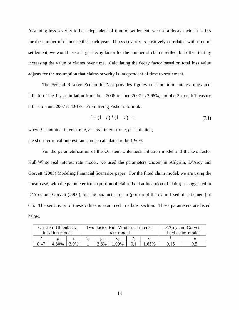
Assuming loss severity to be independent of time of settlement, we use a decay factor a = 0.5

for the number of claims settled each year. If loss severity is positively correlated with time of

settlement, we would use a larger decay factor for the number of claims settled, but offset that by

increasing the value of claims over time. Calculating the decay factor based on total loss value

adjusts for the assumption that claims severity is independent of time to settlement.

The Federal Reserve Economic Data provides figures on short term interest rates and

inflation. The 1-year inflation from June 2006 to June 2007 is 2.66%, and the 3-month Treasury

bill as of June 2007 is 4.61%. From Irving Fisher’s formula:

1)1(*)1( −++= πri (7.1)

where i = nominal interest rate, r = real interest rate, p = inflation,

the short term real interest rate can be calculated to be 1.90%.

For the parameterization of the Ornstein-Uhlenbeck inflation model and the two-factor

Hull-White real interest rate model, we used the parameters chosen in Ahlgrim, D’Arcy and

Gorvett (2005) Modeling Financial Scenarios paper. For the fixed claim model, we are using the

linear case, with the parameter for k (portion of claim fixed at inception of claim) as suggested in

D’Arcy and Gorvett (2000), but the parameter for m (portion of the claim fixed at settlement) at

0.5. The sensitivity of these values is examined in a later section. These parameters are listed

below.

Ornstein-Uhlenbeck inflation model

Two-factor Hull-White real interest rate model

D’Arcy and Gorvett fixed claim model

? µ s ?r µr s r ?l s l k m 0.47 4.80% 3.0% 1 2.8% 1.00% 0.1 1.65% 0.15 0.5

15

8. RUNNING THE MODEL

This model is available on the author’s website and will also be made available through

the CAS website so any interested reader can run the model to reproduce the results here or test

alternative parameters. The loss reserve model, which is designed in Microsoft Excel, begins

with an input worksheet for the user to enter the parameters for each model used and the number

of iterations to be made in the simulation. For each iteration, the model simulates a loss

distribution, a real interest rate path and an inflation path which are used to produce the nominal

and economic loss ranges. An output worksheet collects the values from each iteration and

calculates the mean, standard deviation, and reserve ranges for both the nominal and economic

value cases. Finally a summary sheet shows the key statistics, each parameter used, and the

number of iterations in the simulation in side-by-side columns for comparison.

The model is set to generate 1000 random lognormally distributed claims settled on a

decaying basis over 10 years. The mean and standard deviation of the losses are arbitrarily set to

1000 and 250 respectively. The decay model then calculates the proportion of these claims

settled at each time step up to the 10th year.

The generated losses are compounded at the inflation rate up to their time of settlement.

This is the nominal, undiscounted value of losses that insurers are statutorily required to have in

reserve. The interest rate model generates cumulative interest rate paths corresponding to each

time period up to settlement. The nominal values are then discounted back by this cumulative

interest rate factor to obtain the economic value of losses.

For a simplified example, assume a single claim of $1000 (based on the price level in

effect when the loss occurred) is settled at the end of 5 years, and the annual nominal interest rate

is 5% and inflation is 3% throughout the 5 years. The nominal value of the loss reserve would be

16

$1000 * (1+3%)5 = $1159.27. This nominal value is discounted back by the interest rate over the

5 years to get the economic value $1159.27 * (1+5%)-5 = $908.32. In economic terms, the

amount that should be reserved for handling this loss in today’s dollars is $908.32. But what

happens when the inflation rate changes by 2%? Assuming the real interest rate stays fixed, the

nominal rate will also change by approximately 2%. If the nominal rate is 7% and inflation is 5%,

the nominal value and economic value will be $1276.28 and $909.97 respectively. If the

nominal rate is 3% and inflation is 1%, the nominal value and economic value will be $1051.01

and $906.61 respectively. Thus, the nominal value range will be $1276.28 - $1051.01 = $225.27,

and the economic value range will be $909.97 - $906.61 = $3.36. The economic value range is

only 1.5% of the nominal value range. This is a simplified example illustrating three possible

values of one claim assuming real interest rates stay constant. This shows how much smaller

reserve ranges based on economic values would be then ranges based on nominal values.

Now consider book of 1000 such claims and allow real interest rates to vary

independently of inflation. The average nominal and economic values of these 1000 claims are

determined based on the interest rate and inflation paths generated for that simulation. This

claims generation process is repeated for 10,000 simulations, with each simulation generating a

different interest rate and inflation path for the 1000 claims of that iteration, and a distribution of

nominal and economic loss reserves are generated. The mean, standard deviation, minimum,

maximum, as well as the 5, 25, 75 and 95 percentile for both the nominal and economic loss

ranges are determined and compared. A confidence interval ratio is computed by dividing the

economic range confidence interval by the nominal range confidence interval for both a 50

percent (ranging from the 25th percentile to the 75th percentile) and 90 percent (ranging from the

17

5th percentile to the 95th percentile) confidence interval. These ratios will be a good indicator of

the difference in volatility between the economic loss ranges and nominal loss ranges.

9. RESULTS

For most cases, the 50 percent and 90 percent confidence interval ratios turn out to be

very close, so we will focus on the 90 percent confidence interval ratios here. The complete

results are available from the authors.

9.1 Constant versus stochastic real interest rate

We begin by running the model with a time step of 1 year assuming the Taylor model

(Case A). The real interest rate is held constant as in the example above. The economic reserve

range turns out to be approximately 15% of the nominal loss reserve range. This result differs

from the simple example in the previous section because inflation is not constant until settlement,

but instead it varies as it reverts to its long-term mean while experiencing random shocks. When

real interest rates are also allowed to vary (Case B), its volatility will be factored into the

nominal discount factor, increasing the volatility of the economic range. Notice that this does

not affect the nominal values so the nominal ranges are approximately the same. The results

differ based on process risk as a different sample of claims, interest rates and inflation rates are

generated for each case. The economic reserve range is approximately 38% of the nominal loss

reserve range.

18

Figure 3

Standard Percentiles 90% Confidence Confidence Case Mean Deviation 5th 95th Interval Interval Ratio

A nominal 1015699 51421 1001028 1171356 170328 A economic 946750 7962 933787 959642 25855 0.1518

B nominal 1085461 51265 1003123 1170281 167157 B economic 946546 19514 914699 978931 64232 0.3843

Table 1

9.2 Taylor versus fixed claim

Incorporating the fixed loss model suggested by D’Arcy and Gorvett (2000) significantly

changes the results (Case C). Because losses are only exposed to a portion of the full inflation

rate throughout its time to settlement, the impact of inflation is less than the previous case. This

drastically reduces the volatility of the nominal range. In case B, the effect of discounting the

nominal value to get the economic value is ameliorated by fully inflating the loss to its nominal

value. In fact, the economic value of loss reserves is just the loss discounted by the real interest

rate, ignoring inflation. Thus the volatility of the economic value is affected only by the

19

volatility of the real interest rate. But under the fixed claim model where the losses are not

inflated by the same amount as they are discounted, the volatility of the discount factor will be

the product of the real interest rate volatility and the volatility of inflation that was not used to

inflate the loss. Thus the volatility of the economic value will be larger. Putting it all together,

the fixed claim model uses a smaller volatility to compound the loss to its nominal value but a

larger volatility to discount it back to its economic value. This increases the ratio of the

economic to nominal confidence intervals to roughly 60%.

Figure 4

Standard Percentiles 90% Confidence Confidence Case Mean Deviation 5th 95th Interval Interval Ratio

B nominal 1016003 51265 1003123 1170281 167157 B economic 946546 19514 914699 978931 64232 0.3843

C nominal 1056597 35661 999931 1117435 117505 C economic 924688 21543 889718 960237 70519 0.6001

Table 2

20

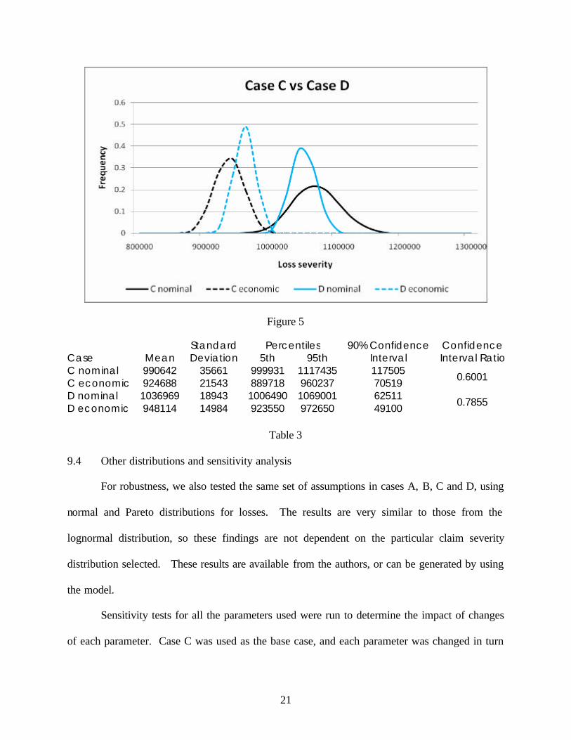
Case C will be the base case used to make comparisons with assumptions we made on the

time step, proportion of claim fixed when settled, and the significance of using an economic

value approach when inflation is high and volatile.

9.3 Time step

The time step determines the frequency at which changes in interest rates occur. When

we use a time step of 1/12th of a year, interest rates will be generated on a monthly basis (Case

D). For the Taylor model, the volatility of both the inflation and nominal rate decreases by

approximately the same amount, thus keeping the confidence interval ratio constant. However,

because losses are compounded by only a proportion of inflation in the fixed claim model, this

inflation volatility will decrease more than the nominal rate using the full inflation. Figure 5

shows that the nominal and economic have more similar shapes. Again, the relative volatility

change between the proportion inflation falls behind the volatility change in the nominal rate,

causing the confidence interval ratio to increase. The results with a time step of 1/12 year show

the confidence interval ratio increases to approximately 79%.

21

Figure 5

Table 3

9.4 Other distributions and sensitivity analysis

For robustness, we also tested the same set of assumptions in cases A, B, C and D, using

normal and Pareto distributions for losses. The results are very similar to those from the

lognormal distribution, so these findings are not dependent on the particular claim severity

distribution selected. These results are available from the authors, or can be generated by using

the model.

Sensitivity tests for all the parameters used were run to determine the impact of changes

of each parameter. Case C was used as the base case, and each parameter was changed in turn

Standard Percentiles 90% Confidence Confidence Case Mean Deviation 5th 95th Interval Interval Ratio C nominal 990642 35661 999931 1117435 117505 C economic 924688 21543 889718 960237 70519 0.6001

D nominal 1036969 18943 1006490 1069001 62511 D economic 948114 14984 923550 972650 49100 0.7855

22

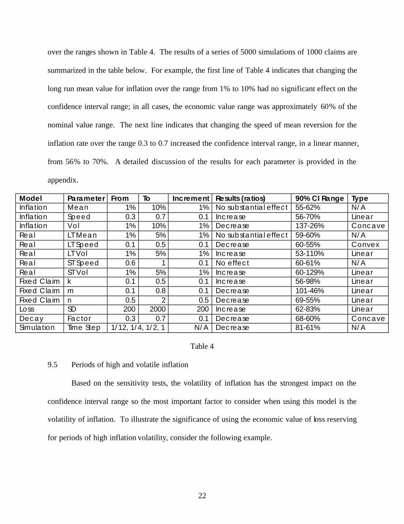
over the ranges shown in Table 4. The results of a series of 5000 simulations of 1000 claims are

summarized in the table below. For example, the first line of Table 4 indicates that changing the

long run mean value for inflation over the range from 1% to 10% had no significant effect on the

confidence interval range; in all cases, the economic value range was approximately 60% of the

nominal value range. The next line indicates that changing the speed of mean reversion for the

inflation rate over the range 0.3 to 0.7 increased the confidence interval range, in a linear manner,

from 56% to 70%. A detailed discussion of the results for each parameter is provided in the

appendix.

Model Parameter From To Increment Results (ratios) 90% CI Range Type Inflation Mean 1% 10% 1% No substantial effect 55-62% N/A Inflation Speed 0.3 0.7 0.1 Increase 56-70% Linear Inflation Vol 1% 10% 1% Decrease 137-26% Concave Real LT Mean 1% 5% 1% No substantial effect 59-60% N/A Real LT Speed 0.1 0.5 0.1 Decrease 60-55% Convex Real LT Vol 1% 5% 1% Increase 53-110% Linear Real ST Speed 0.6 1 0.1 No effect 60-61% N/A Real ST Vol 1% 5% 1% Increase 60-129% Linear Fixed Claim k 0.1 0.5 0.1 Increase 56-98% Linear Fixed Claim m 0.1 0.8 0.1 Decrease 101-46% Linear Fixed Claim n 0.5 2 0.5 Decrease 69-55% Linear Loss SD 200 2000 200 Increase 62-83% Linear Decay Factor 0.3 0.7 0.1 Decrease 68-60% Concave Simulation Time Step 1/12, 1/4, 1/2, 1 N/A Decrease 81-61% N/A

Table 4

9.5 Periods of high and volatile inflation

Based on the sensitivity tests, the volatility of inflation has the strongest impact on the

confidence interval range so the most important factor to consider when using this model is the

volatility of inflation. To illustrate the significance of using the economic value of loss reserving

for periods of high inflation volatility, consider the following example.

23

When inflation rates become high and volatile, nominal loss reserve ranges are drastically

impacted. To demonstrate this, we ran a simulation using a 10% current short term rate and 10%

volatility for the inflation model (Case E). (Using a 10% long term mean instead of 10% current

short term rate produces a similar result.) Unlike case B, the volatility of the nominal discount

factor is now being reduced by the relatively much lower volatility of the real interest rate and is

no longer larger than the compounded inflation factor. The nominal ranges are much larger

under this situation, with the 90% confidence interval increasing from $117,505 to $391,988.

The economic value range also increases, but not nearly as much, from $70,509 to $97,009. The

confidence interval ratio drops to 25%. Thus the problem of using nominal loss reserves to

determine reserve ranges is exacerbated in periods of volatile inflation. The higher the inflation

volatility, the more important it is that economic values be used to set reserves and ranges.

Figure 5

Standard Percentiles 90% Confidence Confidence Case Mean Deviation 5th 95th Interval Interval Ratio

24

C nominal 990642 35661 999931 1117435 117505 C economic 924688 21543 889718 960237 70519 0.6001

E nominal 1100972 119330 915452 1307440 391988 E economic 896529 30055 845077 942086 97009 0.2475

Table 5

9.6 Summary of results

Based on the many simulations run for this research, the economic mean is always

smaller than the nominal mean. Under most circumstances, the economic value reserve ranges

are smaller than the nominal value ranges. This is not always the case under the fixed claim

model, especially when the time steps are small and the claim values become fixed quickly. The

economic value range will be smaller than the nominal value ranges under all circumstances if a

large proportion of the claim is fixed in value at the end of the claim settlement process. During

periods of high inflation, nominal values become far more volatile than economic values, making

the economic value range confidence interval ratio much smaller than the nominal value range.

10. CONCLUSION

Property–liability insurance companies have traditionally valued their loss reserves on a

nominal basis due to statutory requirements. These requirements do not reflect the economic

value of the future payments and distort insurance company financial statements. Nominal loss

reserves overstate the impact of inflation on reserves, as they ignore the relationship between

inflation and nominal interest rates. The economic impact on loss reserves of a change in

inflation is commonly offset by a similar shift in the nominal interest rate. Loss reserve ranges

based on nominal values accentuate this problem. Recent proposal advocate the use of fair value

accounting for loss reserves, which would replace nominal values with economic values. In this

study a loss reserve model was developed to quantify the uncertainty introduced by stochastic

25

interest rates and inflation rates and to compare reserve ranges based on nominal and economic

values. The results demonstrate a variety of scenarios under which the reserve ranges based on

economic values can be either smaller or larger than the nominal value ranges. However, use of

economic values for loss reserves would better serve the insurance industry and its regulators.

The key reason for encouraging the use of economic value ranges is that they properly reflect the

true measure of the uncertainty involved in loss reserving. An additional benefit is that the

ranges are smaller in many circumstances, providing more credible values of the cost and

uncertainty of future loss payments. As the level and volatility of inflation increases, which

appears to occurring currently, the ratio of the reserve ranges based on economic values to the

nominal value ranges declines, increasing the importance of the use of economic values.

26

REFERENCES [1] Actuarial Standards Board, Actuarial Standard of Practice No. 20, “Discounting of

Property and Casualty Loss and Loss Adjustment Expense Reserves,” http://www.actuarialstandardsboard.org/pdf/asops/asop020_037.pdf

[2] Ahlgrim, Kevin, Stephen P. D'Arcy and Richard W. Gorvett, “The Effective

Duration and Convexity of Liabilities for Property-Liability Insurers Under Stochastic Interest Rates,” Geneva Papers on Risk and Insurance Theory, 2004, Vol. 29, No. 1, pp. 75-108.

[3] Ahlgrim, Kevin, Stephen P. D'Arcy and Richard W. Gorvett, “Modeling Financial

Scenarios: A Framework for the Actuarial Profession,” Proceedings of The Casualty Actuarial Society, Vol. XCII, 2005, pp. 60-98.

[4] American Academy of Actuaries, “Fair Valuation of Insurance Liabilities: Principles

and Methods,” 2002, http://www.actuary.org/pdf/finreport/fairval_sept02.pdf. [5] Barnett, Glen and Ben Zehnwirth, “Best Estimates for Reserves,” Casualty Actuarial

Society Forum, Fall 1998, pp. 1-54. [6] Berquist, James R. and Richard E. Sherman, “Loss Reserve Adequacy. Testing: A

Comprehensive, Systematic Approach,” Proceedings of The Casualty Actuarial Society, Vol. LXIV, 1977, pp. 123-184.

[7] Butsic, Robert P., “The Effect of Inflation on Losses and Premiums for Property-

Liability Insurers,” Casualty Actuarial Society Discussion Paper Program, 1981, pp. 58-102.

[8] Butsic, Robert P., “Determining the Proper Interest Rate for Loss Reserve

Discounting: An Economic Approach,” Casualty Actuarial Society Discussion Paper Program, Fall 1988, pp. 147-186.

[9] Casualty Actuarial Society, “Fair Value of P&C Liabilities: Practical Implications,”

2004, http://www.casact.org/pubs/fairvalue/FairValueBook.pdf. [10] Casualty Actuarial Society, “Task Force on Actuarial Credibility,” 2005,

http://www.casact.org/about/reports/tfacrpt.pdf.

[11] CAS Working Party on Quantifying Variability in Reserve Estimates, Casualty Actuarial Forum, Fall 2005, pp. 29-146.

[12] CEA Information Papers, “Solvency II: Understanding the process,” 2007,

http://www.cea.assur.org/cea/download/publ/article257.pdf.

27

[13] D'Arcy, Stephen P., “Revisions in Loss Reserving Techniques Necessary to Discount Property-Liability Loss Reserves” Proceedings of the Casualty Actuarial Society, Vol. 74, 1987, pp. 75-100.

[14] D'Arcy, Stephen and Richard W. Gorvett, “Measuring the Interest Rate Sensitivity of

Loss Reserves, Proceedings Of The Casualty Actuarial Society,” Vol. 87, 2000, pp. 365-400. http://www.casact.org/pubs/proceed/proceed00/00365.pdf.

[15] Federal Reserve Economic Data http://research.stlouisfed.org/fred2/. [16] Fisher, Irving, The Theory of Interest, Macmillan, 1930, Chapter 19. [17] Girard, Luke N., “An Approach to Fair Valuation of Insurance Liabilities Using the

Firm's Cost of Capital,” North American Actuarial Journal, 6:2, 2002, pp. 18–46. [18] Hettinger, Thomas, “What Reserve Ranges Makes You Comfortable,” Midwestern

Actuarial Forum Fall Meeting, 2006, http://www.casact.org/affiliates/maf/0906/hettinger.pdf.

[19] Kirschner, Gerald S., Colin Kerley, and Belinda Isaacs, “Two Approaches to

Calculating Correlated Reserve Indications Across Multiple Lines of Business,” Casualty Actuarial Society Forum, Fall 2002, pp. 211-246.

[20] Mack, Thomas, “Distribution-free Calculation of the Standard Error of Chain Ladder

Reserve Estimates,” AST1N Bulletin, 23:2, 1993, pp. 213-225. [21] McClenahan, Charles L., “Estimation and Application of Ranges of Reasonable

Estimates,” Casualty Actuarial Society Forum, Fall, 2003, pp. 213-230. [22] Miller, Mary Frances, “Are You Part of the Solution,” Actuarial Review, February,

2004, http://www.casact.org/pubs/actrev/feb04/pres.htm. [23] Murphy, Daniel M., “Unbiased Loss Development Factors,” PCAS LXXXI, 1994, pp.

154-222. [24] Narayan, Prakash and Thomas V. Warthen, “A Comparative Study of the

Performance of Loss Reserving Methods Through Simulation,” Casualty Actuarial Society Forum, Summer 1997, pp. 175-196.

[25] Patel, Chandu C. and Alfred Raws III, “Statistical Modeling Techniques for Reserve

Ranges: A Simulation Approach,” Casualty Actuarial Society Forum, Fall 1998, pp. 229-255.

[26] Richards, William F., “Evaluating the Impact of Inflation on Loss Reserves,”

Casualty Actuarial Society Discussion Paper Program, Fall 1981, pp. 384-400.

28

[27] Shapland, Mark R., “Loss Reserve Estimates: A Statistical Approach for Determining

“Reasonableness”,” Casualty Actuarial Society Forum, Fall 2003, pp. 321-360. [28] Standard & Poor’s, “Insurance Actuaries: A Crisis of Credibility,” 2003. [29] Taylor, Greg C., “Separation of Inflation and Other Effects from the Distribution of

Non-Life Insurance Claim Delays,” ASTIN Bulletin, 9:1-2, 1977, pp. 219-230. [30] Venter, Gary G., “Refining Reserve Runoff Ranges,” ASTIN Colloquium, Orlando,

Florida, 2007. [31] Wiser, Ronald F., Jo Ellen Cockley and Andrea Gardner, “Loss Reserving”

Foundations of Casualty Actuarial Science, Casualty Actuarial Society, 2001, Chapter 5, pp. 197-285.

[32] Zehnwirth, Ben, “Probabilistic Development Factor Models with Applications to

Loss Reserve Variability, Prediction Intervals, and Risk Based Capital,” Casualty Actuarial Society Forum, Spring 1994, pp. 447-606.

29

APPENDIX – SENSITIVITY ANALYSIS

For any stochastic model, the number simulations run in a study is an important

determinant. Too few simulations can lead to widely varying results and erroneous conclusions.

Running too many simulations wastes time and computer resources. For simple models,

statistical analysis can be used to determine the appropriate number of simulations to run.

However, in this project, which consists of five separate stochastic models, that approach is not

feasible. Instead, we ran the model multiple times for selected numbers of simulations and

claims and then calculated the variability of the key variable used in this study, the 90%

confidence interval ratio. (This value is the ratio of the 90 percent confidence interval based on

the economic value of loss reserves to the 90 percent confidence interval based on the nominal

value of loss reserves.) We wanted to determine the appropriate number of simulations to run as

well as the number of claims to use in each simulation, so we tried various combinations of the

two parameters. Each combination was run 20 times and the standard deviation of the

confidence interval ratios was calculated. We were looking for the point where the standard

deviation did not continue to decline when additional simulations or claims were used. The

starting point was 1000 simulations and 1000 claims, which generated a standard deviation of

2.38%. As shown below in Table 1-A, increasing the number of claims to 3000 and to 5000 had

little impact on the standard deviation. However, when the number of simulations was increased,

first to 2500, then 5,000 and 7,500, the standard deviation gradually declined to 0.60%. Running

10,000 simulations did not reduce the variability further, so this combination (10,000 simulations

of 1000 claims) was used to run the individual cases (A through E) described in the paper.

30

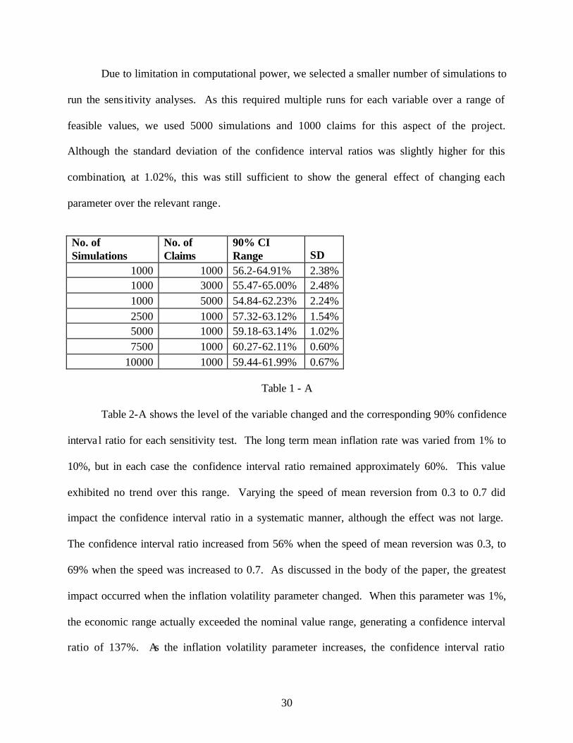
Due to limitation in computational power, we selected a smaller number of simulations to

run the sens itivity analyses. As this required multiple runs for each variable over a range of

feasible values, we used 5000 simulations and 1000 claims for this aspect of the project.

Although the standard deviation of the confidence interval ratios was slightly higher for this

combination, at 1.02%, this was still sufficient to show the general effect of changing each

parameter over the relevant range.

No. of Simulations

No. of Claims

90% CI Range SD

1000 1000 56.2-64.91% 2.38% 1000 3000 55.47-65.00% 2.48% 1000 5000 54.84-62.23% 2.24% 2500 1000 57.32-63.12% 1.54% 5000 1000 59.18-63.14% 1.02% 7500 1000 60.27-62.11% 0.60%

10000 1000 59.44-61.99% 0.67%

Table 1 - A

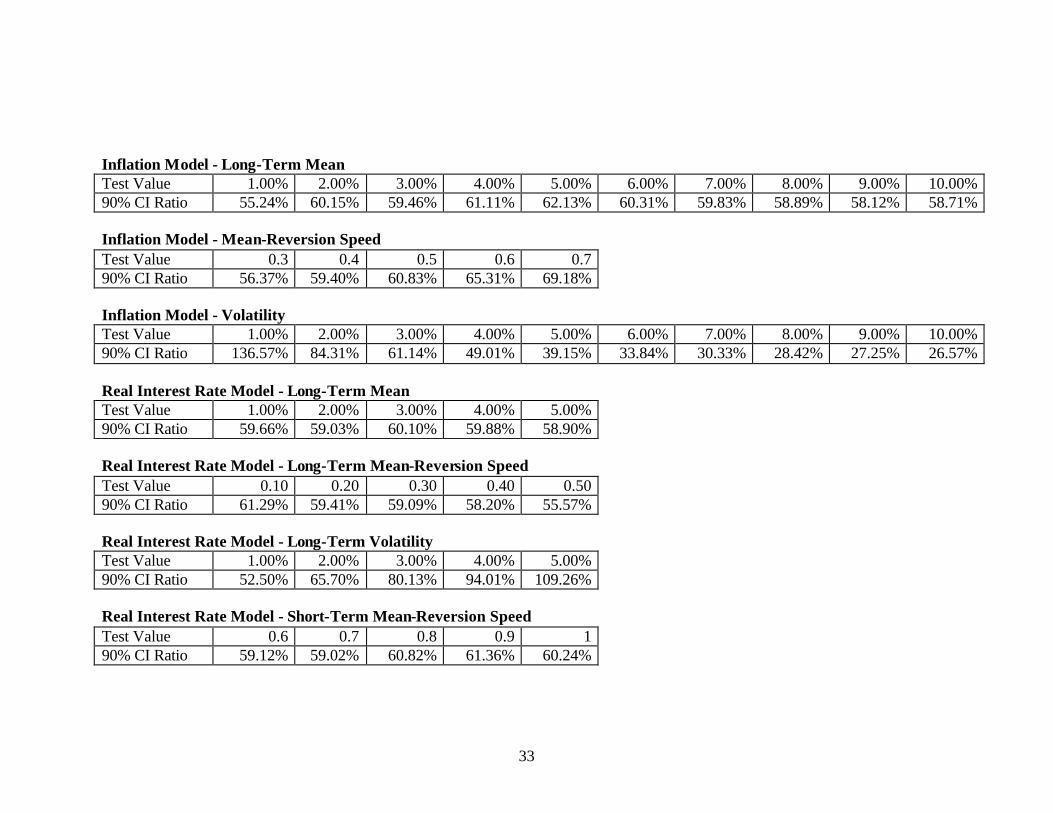
Table 2-A shows the level of the variable changed and the corresponding 90% confidence

interval ratio for each sensitivity test. The long term mean inflation rate was varied from 1% to

10%, but in each case the confidence interval ratio remained approximately 60%. This value

exhibited no trend over this range. Varying the speed of mean reversion from 0.3 to 0.7 did

impact the confidence interval ratio in a systematic manner, although the effect was not large.

The confidence interval ratio increased from 56% when the speed of mean reversion was 0.3, to

69% when the speed was increased to 0.7. As discussed in the body of the paper, the greatest

impact occurred when the inflation volatility parameter changed. When this parameter was 1%,

the economic range actually exceeded the nominal value range, generating a confidence interval

ratio of 137%. As the inflation volatility parameter increases, the confidence interval ratio

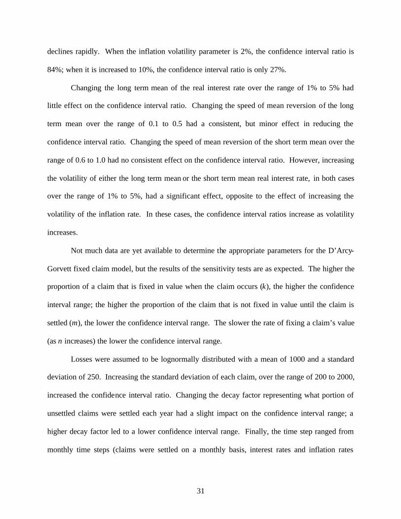
31

declines rapidly. When the inflation volatility parameter is 2%, the confidence interval ratio is

84%; when it is increased to 10%, the confidence interval ratio is only 27%.

Changing the long term mean of the real interest rate over the range of 1% to 5% had

little effect on the confidence interval ratio. Changing the speed of mean reversion of the long

term mean over the range of 0.1 to 0.5 had a consistent, but minor effect in reducing the

confidence interval ratio. Changing the speed of mean reversion of the short term mean over the

range of 0.6 to 1.0 had no consistent effect on the confidence interval ratio. However, increasing

the volatility of either the long term mean or the short term mean real interest rate, in both cases

over the range of 1% to 5%, had a significant effect, opposite to the effect of increasing the

volatility of the inflation rate. In these cases, the confidence interval ratios increase as volatility

increases.

Not much data are yet available to determine the appropriate parameters for the D’Arcy-

Gorvett fixed claim model, but the results of the sensitivity tests are as expected. The higher the

proportion of a claim that is fixed in value when the claim occurs (k), the higher the confidence

interval range; the higher the proportion of the claim that is not fixed in value until the claim is

settled (m), the lower the confidence interval range. The slower the rate of fixing a claim’s value

(as n increases) the lower the confidence interval range.

Losses were assumed to be lognormally distributed with a mean of 1000 and a standard

deviation of 250. Increasing the standard deviation of each claim, over the range of 200 to 2000,

increased the confidence interval ratio. Changing the decay factor representing what portion of

unsettled claims were settled each year had a slight impact on the confidence interval range; a

higher decay factor led to a lower confidence interval range. Finally, the time step ranged from

monthly time steps (claims were settled on a monthly basis, interest rates and inflation rates

32

could vary each month) to annual time steps. Changing this parameter had a significant effect on

the confidence interval ratio. The longer the time step, the lower the ratio. Under monthly time

steps, the confidence interval ratio was 81%; for annual time steps this ratio was 61%.

The purpose of the sensitivity analysis is to indicate which of the many parameters used

in this model have the greatest impact on the results and the conclusions of this paper. In almost

all cases, the conclusion that the use of economic values to determine loss reserves would lead to

smaller reserve ranges is supported. Attention should be focused on measuring the parameters

with the greatest impact on determining loss reserves and their ranges under either nominal or

economic values. Thus, measures of interest rate and inflation volatility and the fixed claim

parameters should be studied closely.

33

Inflation Model - Long-Term Mean Test Value 1.00% 2.00% 3.00% 4.00% 5.00% 6.00% 7.00% 8.00% 9.00% 10.00% 90% CI Ratio 55.24% 60.15% 59.46% 61.11% 62.13% 60.31% 59.83% 58.89% 58.12% 58.71% Inflation Model - Mean-Reversion Speed Test Value 0.3 0.4 0.5 0.6 0.7 90% CI Ratio 56.37% 59.40% 60.83% 65.31% 69.18% Inflation Model - Volatility Test Value 1.00% 2.00% 3.00% 4.00% 5.00% 6.00% 7.00% 8.00% 9.00% 10.00% 90% CI Ratio 136.57% 84.31% 61.14% 49.01% 39.15% 33.84% 30.33% 28.42% 27.25% 26.57% Real Interest Rate Model - Long-Term Mean Test Value 1.00% 2.00% 3.00% 4.00% 5.00% 90% CI Ratio 59.66% 59.03% 60.10% 59.88% 58.90% Real Interest Rate Model - Long-Term Mean-Reversion Speed Test Value 0.10 0.20 0.30 0.40 0.50 90% CI Ratio 61.29% 59.41% 59.09% 58.20% 55.57% Real Interest Rate Model - Long-Term Volatility Test Value 1.00% 2.00% 3.00% 4.00% 5.00% 90% CI Ratio 52.50% 65.70% 80.13% 94.01% 109.26% Real Interest Rate Model - Short-Term Mean-Reversion Speed Test Value 0.6 0.7 0.8 0.9 1 90% CI Ratio 59.12% 59.02% 60.82% 61.36% 60.24%

34

Real Interest Rate Model - Short-Term Volatility Test Value 1.00% 2.00% 3.00% 4.00% 5.00% 90% CI Ratio 59.94% 79.05% 92.99% 116.16% 128.98% Fixed Claim Model - Fixed Portion at time 0 (k) Test Value 0.1 0.2 0.3 0.4 0.5 90% CI Ratio 56.17% 63.73% 71.53% 83.70% 97.76% Fixed Claim Model - Portion unknown until settlement (m) Test Value 0.1 0.2 0.3 0.4 0.5 0.6 0.7 0.8 90% CI Ratio 101.19% 87.83% 74.94% 68.49% 60.75% 56.43% 50.99% 45.73% Fixed Claim Model - Speed of Settlement (n) Test Value 0.5 1 1.5 2 90% CI Ratio 69.02% 61.01% 58.08% 55.20% Loss Model - Standard Deviation Test Value 200 400 600 800 1000 1200 1400 1600 1800 2000 90% CI Ratio 61.61% 63.45% 67.70% 68.40% 74.50% 77.50% 79.91% 81.07% 80.82% 83.39% Decay Model - Decay Factor Test Value 0.3 0.4 0.5 0.6 0.7 90% CI Ratio 67.52% 63.08% 60.57% 60.74% 60.29% Simulation - Time Step Test Value 0.083 0.250 0.500 1.000 90% CI Ratio 80.95% 78.19% 75.17% 61.46%

Table 2-A