Bank of Canada staff working papers provide a forum for staff to publish work-in-progress research independently from the Bank’s Governing Council. This research may support or challenge prevailing policy orthodoxy. Therefore, the views expressed in this paper are solely those of the authors and may differ from official Bank of Canada views. No responsibility for them should be attributed to the Bank. ISSN 1701-9397 ©2020 Bank of Canada

Staff Working Paper/Document de travail du personnel — 2020-56

Last updated: December 23, 2020

Losing Contact: The Impact of Contactless Payments on Cash Usage by Marie-Hélène Felt

Currency Department Bank of Canada, Ottawa, Ontario, Canada K1A 0G9

mfelt@bank-banque-canada.ca

i

Acknowledgements I am grateful to Kim Huynh, Marcel Voia, Fumiko Hayashi, David Drukker and Jeffrey Wooldridge for insightful comments and discussions. I also thank numerous colleagues from the Bank of Canada, in particular Heng Chen, Janet Jiang and Maarten van Oordt, for their feedback. I acknowledge the collaborative efforts of Michael Hsu (Ipsos Reid) for the ongoing development of the section on methods of payment in the Canadian Financial Monitor survey. The views expressed in this paper are mine. No responsibility for them should be attributed to the Bank of Canada.

ii

Abstract I investigate the impact of contactless credit cards (CTCs) on cash use in Canada, using panel data between 2010 and 2017. I show that ignoring unobserved heterogeneity would lead to overstating the impact of CTCs on cash usage in a linear model. Using finite mixture modelling, I provide evidence of the differential impacts of CTCs on the extensive versus intensive margins of cash usage. I use a two-part model, with an exclusion restriction for better identification, to model both margins separately. I obtain that CTC use negatively influences the intensive margin of cash usage but not its extensive margin. There is no clear evidence of an S-curve pattern in the impact of CTCs on cash usage over the sample period.

Topics: Bank notes; Digital currencies and fintech; Econometric and statistical methods; Financial services JEL codes: C33, D12, E41

1 Introduction

In many developed countries, transactional usage of cash is falling or already very low

(Khiaonarong and Humphrey, 2019). At the same time, contactless payments are becom-

ing more prevalent around the globe (see, e.g., Bounie and Camara, 2020). As they mimic

some desirable features of cash, such as speed and ease of use, and are typically used for

smaller value transactions, contactless cards can be posited as a competitive alternative to

cash. This study investigates whether contactless payments are an important contributor to

the decline in transactional usage of cash, based on Canadian evidence. It is important for

central banks to understand the displacement of cash by other payments methods as they

are responsible for issuing and distributing currency and are also increasingly investigating

the possibility of issuing digital currency. More widely, this question is also of interest to

other participants in the payments market such as card processors and merchants.

In Canada and elsewhere, aggregate trends point toward a substitution from cash (on the

decline) to contactless payment methods (on the rise). However, these global trends may be

mistakenly interpreted as evidence of a causal impact of these recent payment innovations on

cash. Regression analyses of micro data provide little evidence that such a causal relationship

exists, in particular when endogeneity issues are properly taken care of using panel data or

randomized experiments. Using panel data from the 2010-2012 Canadian Financial Monitor

(CFM) survey to control for unobserved heterogeneity, Chen et al. (2017) find little or no

reduction in cash usage resulting from the use of contactless credit cards (CTCs).1 Trutsch

(2020) finds evidence that contactless credit and debit cards exert no statistically significant

effect on cash usage, after controlling for unobserved heterogeneity in cash usage using U.S.

panel data for the period 2009-2013. Finally, using more-recent data from a quasi-random

experiment in Switzerland for 2015-2018, Brown et al. (2020) find only a moderate average

reduction in the cash share of payments (0.6 percentage points relative to an average cash

1They find no significant impact in the 2010-2011 two-year panel or the 2010-2012 three-year panel, andonly a 3 percent reduction in the cash share in value in the 2011-2012 two-year panel.

1

share of 68 percent) following the receipt of contactless debit cards.

In this paper I explore panel data on methods of payment obtained from the CFM

survey for the 2010-2017 period to investigate the impact of CTCs on transactional cash

usage. My main contributions are the following: (i) I update available estimates of the

effect of payment innovations on cash usage, using recent data; (ii) I make use of a unique

panel data set that covers a period of eight years and assess how these estimates may have

varied over the sample period; (iii) I investigate heterogeneity in the impact of CTCs on cash

usage across households, using finite mixture modelling (FMM); (iii) instead of the linear

panel model typically used in the aforementioned literature, I motivate employing a two-part

model that properly takes into account the corner-solution nature of the dependent variable

“cash share.”

In Canada, the share of cash in overall retail payments has decreased continuously over

the past 20 years. While an overwhelming majority of Canadian consumers now have access

to debit or credit cards, they can also choose from a wide set of retail payment innovations

to use at the point of sale ( see, e.g., Arango et al., 2012; and Henry et al., 2018). One such

innovation is near-field communication-enabled payment cards. These contactless cards allow

consumers to make payments below a certain value by waving their card in front of a payment

terminal (“tap-and-go”), without entering a personal identification number (PIN).

CTCs were first introduced in Canada in 2006 (MasterCard’s PayPass) and 2007 (Visa’s

payWave). The diffusion of CTCs among cardholders happened gradually, in conjunction

with the replacement of previous magnetic stripe cards with chip credit cards over the 2007-

2015 period. Concurrent to these developments on the consumer side was the gradual de-

ployment of contactless payment terminals at merchants, driving the increased acceptance

of contactless payments. According to Technology Strategies International (2017), over the

period 2013-2018, the number of contactless-enabled payment terminals grew on average by

24 percent yearly. In fact, contactless terminals are now the default option when acquiring

a new device and if merchants do not want to accept contactless payments, then they must

2

disable this function.

More recently, Interac debit cards with a contactless payment feature (Flash) entered

the retail payment market. They were first introduced by a limited number of financial

institutions in the autumn of 2011. Although the rollout of contactless debit cards (CTDs)

is well underway, as all main financial institutions now offer them, ownership of Interac Flash

enabled cards is dependent on banks’ rate of replacing their customers’ older debit cards with

new contactless ones.

The remainder of the paper is organized as follows. Section 2 describes the data set.

Section 3 provides descriptive statistics on CTC and cash usage over the 2010-2017 period.

Section 4 presents estimation results, using a standard linear panel model, for the impact

of CTCs on cash usage. Section 5 presents an FMM analysis that motivates the separate

modelling of the extensive and intensive margins of cash usage. In Section 6, using a corner-

solution model, I estimate the differential impact of CTCs on the extensive and intensive

margins of cash usage. Section 7 concludes.

2 Canadian Financial Monitor panel data

The CFM is an annual survey of Canadian households’ finances, which Ipsos Reid has been

conducting since 1999. A module concerning methods of payment usage was introduced by

the Bank of Canada in the CFM questionnaire in 2009. This module uses recall questions

to collect information on payment choices and cash management. Respondents are invited

to assess their past or “typical” behaviour with respect to the methods of payments they

use for making purchases, the frequencies and amounts of their cash withdrawals, and their

cash holdings. The methods-of-payment module and, in particular, the questions on cash

usage underwent major changes between 2009 and 2010, and 2017 and 2018. To avoid major

breaks in the data series, I use the CFM data for 2010-2017 for the present analysis.2

2The recall question for cash purchases was changed from the past month to the past week in January 2010and changed back to the past month in January 2018. The paper-based household CFM was discontinued

3

The annual size of the CFM sample is approximately 12,000 households. The sampling

and weighting procedures aim to obtain annual representations of the Canadian population.

A household can receive only one CFM questionnaire in each 12-month period. However,

because past participants are re-invited to participate in following years, the data has a

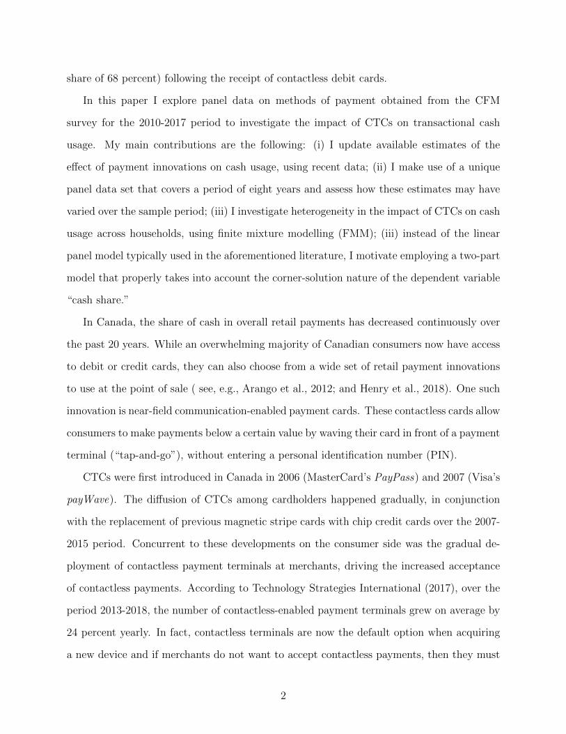
panel dimension. Figure 1 presents the participation patterns of households over the 2010-

2017 period. In total, 40,448 households participated at least once over the 8-year period,

approximately half of which participated more than once, contributing to 94,155 household-

year observations. However, only 1,449 households participated 8 years in a row. This implies

that working on the balanced 8-year panel would severely reduce the sample size. Also, the

households that stayed in the sample over the whole period differ substantially from others

that participated less regularly.

Attrition is less severe when shorter panels are considered. For example, among the

approximately 12,000 households that participated in a given year, about 50 percent par-

ticipated again in the following year while only about 30 percent did so again in the two

following years. To take advantage of the available panel dimension but limit the impact of

attrition, in my analysis I exploit the seven consecutive two-year panels between 2010 and

2017: 2010-2011, 2011-2012, through to 2016-2017.3 This approach also introduces flexibil-

ity in my model as its allows the impact of CTCs on cash usage to vary over time. Indeed,

regression coefficients as well as individual fixed effects terms are assumed constant over

two-year periods instead of the whole eight-year observation period.

3 Cash and contactless credit card usage over the years

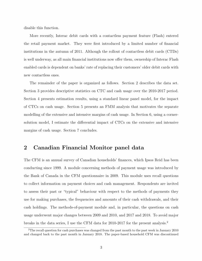
Figure 2 presents methods of payment market shares, by volume, as measured in the Cana-

dian Financial Monitor. The volume share of a given method of payment is the number

of purchases made with that method over the total number of purchases made in a given

in December 2018 and replaced by an online survey (see Felt and Laferriere, 2020).3Chen et al. (2017) find that attrition correction has little effect on estimates for the impact of CTCs on

cash obtained on two-year panels.

4

reference period.4 The figure shows a downward trend in the share of cash usage at the

point of sale over the observation period. Most of the loss in the market share of cash went

to credit cards and CTCs in particular, with a quadrupling of the volume share of CTC

transactions for the period 2010-2017. While the share of overall debit card transactions was

relatively stable over the period, we observe an uptake in the use of CTDs in later years. To

illustrate the concurrent increase in the acceptance of contactless payments, Figure 2 also

reports estimates of the number of contactless terminals deployed in Canada, as published

in Technology Strategies International (2017).

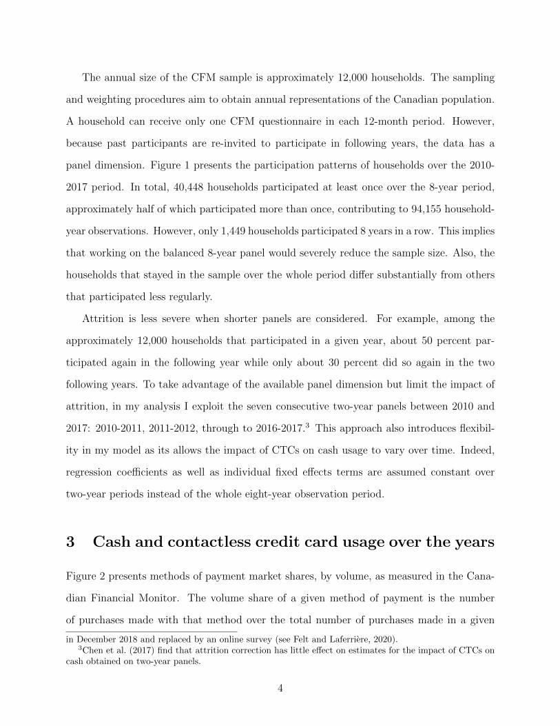
Overall, aggregate trends point toward a substitution from cash to CTCs. Additional

evidence that CTC use leads to a reduction in cash usage is shown in Figure 3, which depicts

the average cash shares, in volume and value, of CTC users and non-users for the period

2010-2017. A CTC user is a household that used a CTC at least once in the past month.

Equivalent to the volume share (defined above), the cash value share is the ratio of the total

value of cash purchases to the total value of all purchases made over the same period. Cash

usage is more prevalent in terms of volume than value, given that cash is mainly used for

small-value transactions. In 2017, the average CTC non-user household paid in cash for

around 31 percent of the total volume of their purchases and 22 percent of the total value

of their purchases. These numbers are down from 42 percent and 28 percent, respectively,

in 2010. CTC users spend on average relatively less cash than non-users. It is interesting to

note that the difference in the cash shares of CTC users and non-users remains at around 10

percentage points over the observation period, despite the increasing intensity of CTC use

by the CTC users observed in Figure 4.

Figure 4 provides statistics on the share of CTC users as well as their mean usage in

terms of volume and value over the 2010-2017 period. For all three measures, we observe

slow growth in the first half of the period and a clear inflexion point in the middle of the

4As cash is mainly used for small-value transactions, the adoption of new modes of payment shouldpredominantly affect cash shares in volume rather than in value. Therefore, in this paper I focus on explainingcash shares by volume.

5

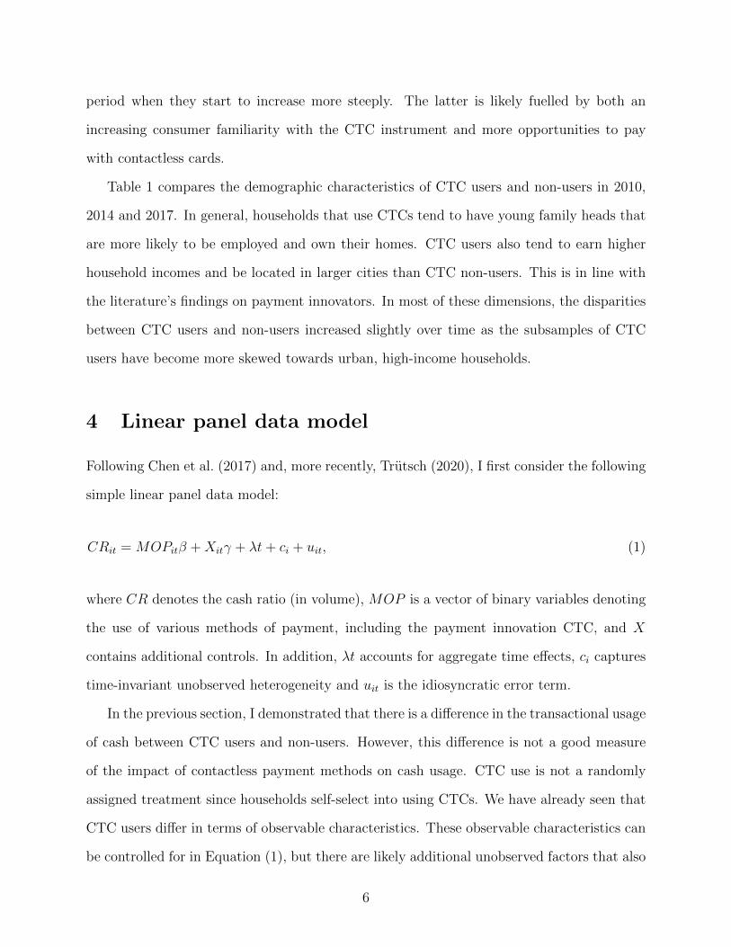
period when they start to increase more steeply. The latter is likely fuelled by both an

increasing consumer familiarity with the CTC instrument and more opportunities to pay

with contactless cards.

Table 1 compares the demographic characteristics of CTC users and non-users in 2010,

2014 and 2017. In general, households that use CTCs tend to have young family heads that

are more likely to be employed and own their homes. CTC users also tend to earn higher

household incomes and be located in larger cities than CTC non-users. This is in line with

the literature’s findings on payment innovators. In most of these dimensions, the disparities

between CTC users and non-users increased slightly over time as the subsamples of CTC

users have become more skewed towards urban, high-income households.

4 Linear panel data model

Following Chen et al. (2017) and, more recently, Trutsch (2020), I first consider the following

simple linear panel data model:

CRit = MOPitβ +Xitγ + λt+ ci + uit, (1)

where CR denotes the cash ratio (in volume), MOP is a vector of binary variables denoting

the use of various methods of payment, including the payment innovation CTC, and X

contains additional controls. In addition, λt accounts for aggregate time effects, ci captures

time-invariant unobserved heterogeneity and uit is the idiosyncratic error term.

In the previous section, I demonstrated that there is a difference in the transactional usage

of cash between CTC users and non-users. However, this difference is not a good measure

of the impact of contactless payment methods on cash usage. CTC use is not a randomly

assigned treatment since households self-select into using CTCs. We have already seen that

CTC users differ in terms of observable characteristics. These observable characteristics can

be controlled for in Equation (1), but there are likely additional unobserved factors that also

6

influence CTC and cash usage. For example, households that are tech savvy may tend to

adopt CTCs more easily but, regardless of whether they adopt this payment method, they

may also tend to dislike cash and use it less intensively than other households. Instead of

comparing cash shares across different households, a better measure of the impact of CTCs

is obtained by assessing how much households’ cash ratios change after they start or stop

using CTCs. Although all concerns about potential sources of bias do not disappear, they

are strongly mitigated by comparing within-household variations. Of course, this requires

panel data.

Once transformed to difference out the unobserved heterogeneity term ci, Model (1)

becomes

∆CRit = ∆MOPitβ + ∆Xitγ + λ+ ∆uit. (2)

I estimate Equation 2 separately on the seven consecutive two-year panels for the period 2010-

2017. This allows for time-varying coefficients, which is especially relevant in the context of

the rapidly changing retail payment landscape that prevails over the period. In particular,

the process of innovation diffusion has an uneven time pattern that is often described using

S-curves. One may therefore expect CTCs to have different effects on cash at different stages

of the innovation dissemination among consumers and merchants.

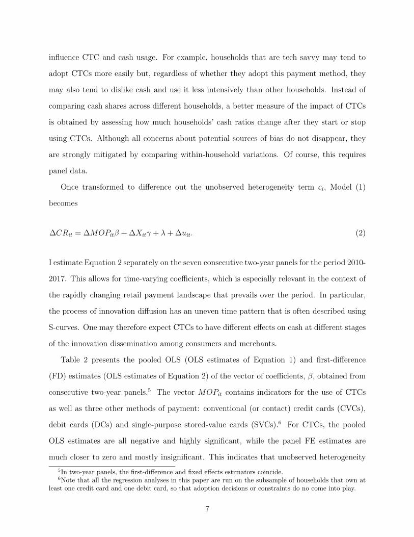
Table 2 presents the pooled OLS (OLS estimates of Equation 1) and first-difference

(FD) estimates (OLS estimates of Equation 2) of the vector of coefficients, β, obtained from

consecutive two-year panels.5 The vector MOPit contains indicators for the use of CTCs

as well as three other methods of payment: conventional (or contact) credit cards (CVCs),

debit cards (DCs) and single-purpose stored-value cards (SVCs).6 For CTCs, the pooled

OLS estimates are all negative and highly significant, while the panel FE estimates are

much closer to zero and mostly insignificant. This indicates that unobserved heterogeneity

5In two-year panels, the first-difference and fixed effects estimators coincide.6Note that all the regression analyses in this paper are run on the subsample of households that own at

least one credit card and one debit card, so that adoption decisions or constraints do no come into play.

7

drives the results obtained from the pooled data and confirms previous findings by Chen

et al. (2017) and Trutsch (2020) about the importance of controlling for it.7 Bias correction

also goes in the same direction for CVCs but in the opposite direction for DCs and SVCs:

the estimates of the latter’s effects on cash usage tend to be more negative when unobserved

heterogeneity is controlled for. This implies that unobserved factors lead a household to use

(i) credit cards more (both CTCs and CVCs) and cash less and (ii) DCs, SVCs and cash

less. Such factors could for example be attitudes towards technology or card rewards. When

significant, the impact of CTCs on cash is around 2 percent and therefore much smaller

than the impact of CVCs (about 10 percent) or even DCs (about 5 percent). This result

is in the same order of magnitude to what was found by Chen et al. (2017) on CFM data

for 2010-2012. In short, after controlling for unobserved heterogeneity in order to mitigate

endogeneity issues, the estimated impact of CTCs on cash usage is very small.

Notice that β in Equation 2 is identified by households with ∆MOP 6= 0 (“switchers”).8

More specifically, the variance of the CTC parameter estimate is inversely proportional to

the number of CTC switchers, including new users with ∆CTC = 1 and stopped users with

∆CTC = −1. The large standard errors of the FE estimates for CTCs could therefore stem

from the small number of CTC switchers in the data. Figure 5 shows the number of CTC,

CVC, DC and SVC switchers and non-switchers in three two-year panels. There are more

CTC switchers than CVC or DC switchers in the data; however, there are slightly more SVC

switchers (especially stopped users). This indicates that the small statistical significance of

the FE parameter estimates for CTCs does not originate from a lack of switchers in the data.

7Unobserved heterogeneity is systematically controlled for in all subsequent models estimated in thispaper. In linear models, time invariant terms are differenced out. For the non-linear two-part model ofSection 6, the Chamberlain-Mundlak device is used to model unobserved heterogeneity; see Equation (5).

8To be precise, given that CVC use is also controlled for, the identification of the impact of CTCs relieson households that switch their CTC but not their CVC use. The latter are mostly those who always useCVCs, both at t− 1 and t. The use of CVCs must be controlled for, otherwise the impact of CTCs could beconfounded with the impact of using credit cards and this would bias the results.

8

5 Exploratory analysis using finite mixture modelling

The analysis in the previous section shows that when estimating the impact of CTCs on

cash usage, it is crucial to allow for household-specific intercept terms. However, Model (2)

assumes complete slope homogeneity. This homogeneity assumption is easily violated if

important interactions are missing from the model. For instance, if they have various levels

of technology preferences, then different new users of CTCs could modify their cash usage

differently. In this section I investigate more-flexible modelling assumptions that allow for

unobserved slope heterogeneity–meaning that the source of the slope heterogeneity is not

observed or not known a priori.

Complete slope heterogeneity (when each cross-sectional unit has its own coefficients) can

be permitted in the context of panel data with a long enough time dimension. Alternatively,

group heterogeneity assumes that cross-sectional units can be classified into a small number

of groups with homogeneous slopes within each group and heterogeneity across groups, but

both the number of groups and the individual memberships in each group are unknown.

I use finite mixture modelling to explore group heterogeneity.9 Each household is assumed

to belong to one of several latent groups, each of which has its own distribution. As a result,

the data is generated by a weighted sum, or mixture, of the different groups’ distributions.

10 However, both the number of groups and the density of each one must be specified.

I first normalize the distribution of the cash ratio variable by applying the inverse hy-

perbolic sine transformation ihs(y) = log(y + (y2 + 1)1/2). This transformation is close to

the log transformation as ihs(y) ' log(2y), but it has the advantage of being defined at zero

(ihs(0) = 0). I then use a normal mixture model applied to first-differenced data, thus still

controlling for time-invariant unobserved heterogenenity.

9The reader is referred to McLachlan et al. (2019) for a short and recent review of finite mixture modelsand to McLachlan and Peel (2004) for a more thorough treatment.

10The finite mixture approach is semi-parametric inasmuch as it does not require any distributional as-sumptions for the underlying mixing distribution (mixing probabilities or weights). Finite mixture modelscan also be viewed as nonparametric approximations to more general mixture models (see, e.g., Laird, 1978;Lindsay, 1983; and Heckman and Singer, 1984). Alternative approaches based on machine learning clusteringtechniques also exist; see Wang et al. (2018) and references therein.

9

Formally, for group g ∈ {1, ..., G}, where G is the number of components in the mixture

(the number of groups among the population),

∆ihs(CRit) = ∆MOPitβg + ∆Xitγg + λg + ∆ugit, (3)

where ∆ugit is assumed to be normally distributed with variance Σg. The density of ∆ihs(CRit)

is given by

f(∆ihs(CRit)|∆MOPit,∆Xit, β, γ) =G∑

g=1

πgfg(∆ihs(CRit)|∆MOPit,∆Xit, β, γ),

where πg denotes the (prior) probability for the gth latent group and fg(.) is its density.

For each consecutive two-year panel, I fit finite mixture models with G = 1, G = 2

and G = 3 groups via maximum-likelihood estimation. Slope heterogeneity is evidenced

and, based on Akaike’s and Schwarz’s Bayesian information criteria (AIC and BIC), the

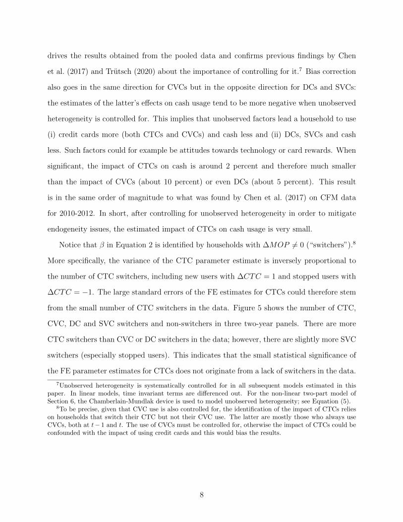
two-component model best suits the data.11 Table 3 presents the regression results of the

two-class model estimation.

For each two-year panel, the procedure identifies one group with large prior probabilities

(between 0.78 and 0.62) and small variances (labelled “Group 1”), and one group with small

prior probabilities (between 0.22 and 0.38) and much larger variances (labelled “Group 2”).

Households in the two FMM groups differ in terms of the impact of CTCs on cash: For

households in Group 1, the CTC parameter estimates are negative with relatively small

standard errors, while for households in Group 2, the CTC parameter estimates are positive

with large standard errors. I estimate that CTC use significantly decreases the cash usage

of households in Group 1, at the 10 percent significance level, in all but two of the seven

two-year panels. In fact, all of the methods-of-payment indicators included in MOP tend to

have significant negative parameter estimates for households in Group 1; but for households

11When run with three latent classes, the maximum-likelihood estimation based on the EM algorithm doesnot always converge.

10

in Group 2, only the CVC coefficients are statistically different from zero.

Having estimated the parameters of the regression mixture, for each household I compute

the posterior probability of belonging to each group and I assign each household to one of

the two FMM groups. A household is assigned to Group 1 if the posterior probability of

belonging to Group 1 is greater than 0.5; it is assigned to Group 2 otherwise. The stacked

histograms in Figure 6 show how each group contributes to the distribution of the dependent

variable ∆ihs(CRit) for the 2010-2011 and 2016-2017 panels. Group 1 models the centre of

the distribution, while Group 2 covers the two long tails of the empirical distribution. More

precisely, Group 1 is mainly composed of households with zero cash ratios at both t− 1 and

t or with positive cash ratios at both t− 1 and t.12 These households experience no change

in the extensive margin of cash usage; only the intensive margin is at play–when there is any

change at all in cash usage. By contrast, Group 2 is mainly composed of households with

CRi(t−1) > 0 and CRit = 0 (in the left tail of the empirical distribution) or CRi(t−1) = 0 and

CRit > 0 (in the right tail of the empirical distribution). In other words, these households

experience a change in cash usage that involves the extensive margin.

These observations lead me to hypothesize that the estimated differential impacts of

CTCs on the two groups of households, using the FMM analysis, in fact reflect the differential

impacts of CTCs on the extensive and intensive margins of cash usage. Figure 7 hints at the

possibility that CTCs have different effects on the extensive and intensive margins of cash

usage. This figure shows the proportion of CTC users by level of cash ratios, where positive

CR values are grouped into five quintile-based bins. It can be observed that, although the

average rate of CTC users increases as cash usage becomes less intensive, this apparent

linear relationship breaks at zero. The next section presents a formal investigation of the

differential effects of CTCs on the extensive and intensive margins of cash usage.

12To be precise, for two years in a row, these households stated they used no (resp. some) cash in thepast week. In the CFM, the recall question on cash purchases concerns the past week: “In the past week,did your household use cash to make purchases?” Questions relative to other methods of payment refer tousage during the past month.

11

6 Corner-solution panel data model

6.1 Modelling cash shares using a two-part model

An important feature of the cash ratio distribution, as can be observed in Figure 8, is the

large mass at zero. In fact, the proportion of zeros in the data gradually increased over

the years, to reach almost one quarter of the sample in 2017. The high incidence of zero

usage, together with a roughly continuous distribution over (0, 1], makes the cash share a

corner-solution outcome.

This type of outcome is often modelled using two-part models that are based on the

statistical decomposition of their densities in separate processes that generate zeros and

positive values; see, for example, Deb and Norton (2018) and Wooldridge (2010), where a

thorough treatment of the econometrics of corner solutions can be found. By modelling

the “participation” (the first-part binary decision) and “amount” (the second-part value

decision, if positive) separately, these models allow for heterogeneous effects of covariates on

the extensive and intensive margins of the decision-making process. One reason why zero

and non-zero values of the cash ratio may arise through two different mechanisms is the

existence of fixed costs that affect “participation.” In the case of cash usage, cash must

necessarily be obtained before it can be spent. The shoe-leather costs of going to the bank

teller or the ATM to withdraw cash as well as potential banking and withdrawal fees are

fixed costs that must therefore be incurred before cash can be used to pay for items at the

point of sale.

Table 4 shows the difference in cash management behaviours across households with zero

and non-zero cash ratios in the past week. Households that reported using some cash for

making purchases in the past week also held more cash in their wallets or purses, made more

cash withdrawals in the past month and reported withdrawals that were typically larger in

size than households that used no cash to make purchases in the past week. In addition,

they were much more likely to be cashless in one of the following ways: holding no cash in

12

their wallets or purses right now, making no ATM withdrawals in the past month or making

no withdrawals from any source in the past month.

These cash management practices further reveal that households with zero and non-zero

cash ratios in the past week face different costs for obtaining cash. In the classic Baumol-

Tobin cash inventory model, consumers optimize their cash management behaviour so as to

minimize the sum of the cost of holding money and the cost of withdrawing cash (including

the opportunity cost of the travel and banking time and banking fees). This model predicts

that the optimal withdrawal frequency decreases with the relative withdrawal cost (i.e., the

cost per dollar spent), while both the withdrawal size to cash consumption ratio (W/c) and

the average cash holdings to cash consumption ratio M/c increase with that cost.13 The

latter two ratios cannot be measured at t for households with CRt = 0. But by making use

of the panel dimension of the data set, I can evaluate these ratios at t− 1 on the subsample

of households with CRt−1 > 0. These values are reported in the last two rows of Table 4.

My results indicate that households with zero cash ratios in year t have fewer withdrawal

frequencies (at time t) and larger W/c and M/c ratios (when defined at time t − 1) than

households with positive cash ratios in year t. This implies that the former households

behaved as if they faced higher cash withdrawal costs than the latter. So withdrawal costs

could indeed play a role in the mechanisms leading to zero and non-zero values of the cash

ratio.

To reformulate the cash ratio equation in the framework of a two-part model, I write

CRit = qit · CR∗it, where qit is a binary variable equal to one if CRit > 0, zero if CRit = 0;

and CR∗it is a continuous, nonnegative, latent variable that is observed only when qit =

1. Different parametric specifications of the two-part model have been proposed in the

literature. Following Cragg (1971) and Duan et al. (1984), I specify the binary variable qit

using a probit model and the latent variable CR∗it using a log-normal distribution. This

model is sometimes referred to as the log-normal hurdle model. The observed variable CRit

13Details of the derivations are available in the Appendix.

13

can then be expressed as

CRit = 1[MOPitβ1 +Xitγ1 + c1i + u1it > 0] exp(MOPitβ2 +Xitγ2 + c2i + u2it), (4)

where u1it|(MOPi, Xi, c1i) ∼ Normal(0, 1) and u2it|(MOPi, Xi, c2i) ∼ Normal(0, σ2u2). As for

the notation, Xi denotes a vector that contains Xit for all t (in my case, for each two-period

panel, t takes only two different values).

In this non-linear model, the unobserved heterogeneity terms c1i and c2i cannot simply

be differentiated out. The correlated random effects (CRE) approach, which dates back

to Mundlak (1978) and Chamberlain (1980), consists in modelling the conditional distribu-

tion of heterogeneity, given the observable covariates. This allows some dependence between

cki and Wi = (MOPi, Xi), for k = 1, 2, which is contrary to the random effects assump-

tions. Wooldridge (2010) applies the CRE approach to various panel data models, including

corner-solution models. Let cki = ψk +W iηk + ak for k = 1, 2, where W i = T−1∑T

r=1Wir is

the vector of the time averages, and ak|Wi ∼ Normal(0, σ2ak). I can rewrite Equation 4 as

CRit = 1[MOPitβ1 +Xitγ1 +W iη1 + v1it > 0] exp(MOPitβ2 +Xitγ2 +W iη2 + v2it), (5)

where v1it|Wi ∼ Normal(0, σ2a1), v2it|Wi ∼ Normal(0, σ2

a2 + σ2u2), and v1i and v2i are indepen-

dent conditional on Wi.

Even though it does not crucially depend on it, the identification of Model 5 is stronger

with an exclusion restriction; i.e., a variable that appears in the participation equation but

not in the amount equation. Due to their physical nature, bank notes and coins must be

obtained before they can be spent. Canadians’ main sources of cash are automated banking

machines (ABM) and bank teller withdrawals, each of which has associated per-transaction

costs. These include shoe-leather costs, which are the travel costs to the source of cash.

Because they are fixed costs, shoe-leather costs should affect the binary participation

decision on whether to use cash as a method of payment via the necessary preliminary

14

decision of whether to obtain cash. However, these costs should be less relevant for explaining

the weekly amount of cash spent. This exclusion restriction is pertinent, given the context

of low and stable inflation, low interest rates and the low risk of holding cash that prevailed

in Canada during the period of analysis.14 In such an environment, where consumers can

carry cash at very low cost, the amount of cash spent (if cash is withdrawn) should mainly

depend on personal preferences and merchant-side factors, rather than on withdrawal cost

considerations.15

Geography is important for explaining consumer banking and cash management choices.

Allen et al. (2008) and, more recently, Choi and Loh (2019) find that a reduction in retail

branch density or an increase in the travel distance to ABMs encourage online banking

adoption and usage.16 Lippi and Secchi (2009) find that, for a given value of cash purchases,

a higher density of bank branches and ABM networks reduces consumers’ average cash

holdings, implying an increase in their withdrawal frequency. Using a more-precise measure

of travel costs to bank branches, Chen et al. (2020) also show that consumers who face

shorter travel distances tend to withdraw more frequently.

I use as an exclusion-restriction variable a distance-based measure of shoe-leather costs,

the distance to the closest bank branch, calculated by Chen and Strathearn (2020); see the

Appendix for details. A potential concern is that consumers’ distance to the closest branch

may not be exogenous to the consumers’ decisions about withdrawing and using cash: local

bank branching decisions could be at least partly driven by local consumers’ payment and

cash management behaviours. For instance, branch closures could very well follow decreases

in consumers’ branch visits due to consumers going cashless. In the context of online banking

adoption, Allen et al. (2008) show evidence that branch closures encourage rather than

14Canadians consider cash as secure to hold and use for payments; see Henry et al. (2018) for assessmentsand objective measures of fraud and security risks for cash and other methods of payments.

15However, for a given amount of cash spending, the fixed withdrawal costs should affect the averageamount withdrawn.

16As online banking substitutes for offline banking, consumers visit branches less frequently. In Alvarezand Lippi’s 2009 generalization of the Baumol-Tobin model, this would correspond to a decrease in theprobability of free (or low-cost) withdrawal opportunities.

15

follow changes in consumer behaviour. Also, considering the potential sluggishness in bank

branching processes, the short time horizon of the analysis (working on two-year panels)

lessens the concern that observed changes in travel distance happen in response to coincident

observed changes in consumers’ behaviour.17

6.2 Differential impacts of contactless credit cards on the exten-

sive and intensive margins of cash usage

The CRE log-normal hurdle model in Equation 5 is estimated using maximum likelihood,

and cluster robust inference is applied to account for serial correlation. Table 5 presents

the estimation results. It reports the marginal effects of CTCs and other payment methods

on (i) the probability of using cash Pr(CR ≥ 0|W,Z) (the extensive margin), (ii) the mean

of the latent amount variable E(CR∗|W ) (the intensive margin), and (iii) the mean of the

observed outcome variable E(CR|W,Z) (the overall effect). Also displayed are the marginal

effects of the instrument, the log-transformed distance to the closest branch, on (i) and (iii).

I find that CTCs affect the intensive margin more than the extensive margin of cash usage.

This payment method’s marginal effects on the probability of using cash are positive, with

large standard errors, while on the latent amount variable they tend to be negative and often

significant (at the 10 percent significance level). It is notable that the three other methods

of payment controlled for also play no significant role in explaining the extensive margin of

cash usage. By contrast, the shoe-leather cost variable matters. As can be observed in the

last panel of Table 5, an increase in the distance to the closest branch significantly decreases

the probability of using cash.

Although the estimates fluctuate a bit over time and are not significant in each two-year

panel, there is clear evidence that CTC use negatively influences the intensive margin of cash

usage. This finding supports the hypothesis formulated before that the significant impact

17An ideal instrument would be completely exogenous, such as a natural disaster that destroys physicalbank branches.

16

of CTCs on cash revealed by the FMM analysis for one sub-group of the population in fact

reflects the effect of CTCs on the intensive margin of cash usage.

The “unconditional” mean of the corner-solution response E(CR|W ) stems from the

combined effects of the extensive and intensive margins of cash usage. As reported in Table 5,

I estimate that CTCs negatively and highly significantly influence the final corner-solution

outcome on most of the seven two-year panels. These estimates are slightly more negative

than the fixed effect estimates of the linear panel model. Still, the estimated impact of CTCs

on E(CR|W ) are relatively low, at about 3 percent.

Overall, the estimates obtained are rather unstable over time. In search of an S-curve

pattern in the impact of CTCs on cash (intensive margin), it can be observed that the

most negative estimates are obtained on the 2015-2016 panel. Next, in the 2016-2017 panel,

the magnitude of the measured CTC impact falls suddenly by half but remains significant.

More-recent data would be needed to confirm whether the years 2015-2016 really mark an

inflection point and delineate an S-curve in the time profile of the impact of CTCs on cash

usage.

7 Conclusion

Understanding the decline in cash use at the point of sale is important for central banks as

well as private stakeholders. In this paper, I investigate the impact of CTCs on cash usage

in Canada by exploring panel data on methods of payment for the period 2010-2017. My

approach differs from previous research in that I employ a corner-solution model to analyze

cash share. My findings can be summarized as follows:

First, unobserved heterogeneity matters when assessing the impact of CTCs on cash us-

age. I control for time-invariant unobserved heterogeneity by exploiting the panel dimension

of the data and show that ignoring this heterogeneity would lead to overstating the impact

of CTCs.

17

Second, CTCs have different effects on the extensive versus the intensive margins of cash

usage. Exploratory analysis based on FMM finds differential impacts of CTCs for two groups

of households, depending on whether they experience changes in the extensive or intensive

margins of their cash usage.

Third, although the estimates are not very stable over time, there is clear evidence that

CTC use negatively influences the intensive margin of cash usage but not its extensive

margin. To model both margins separately, I use a two-part model that properly takes into

account the corner-solution nature of the outcome variable cash share, together with an

exclusion restriction for better identification.

Fourth, the overall impact of CTCs on the transactional usage of cash in Canada is very

small over the 2010-2017 period. While estimates from the two-part model are slightly more

negative than those from the linear panel model, their magnitude is still very small, at about

3 percent.

My results are in line with previous findings for Canada (Chen et al., 2017) and also

findings for the U.S. for the period 2009-2013 (Trutsch, 2020) and Switzerland for 2015-2018

(Brown et al., 2020). Further research is required to unfold which displacement effects are

actually taking place between cash, conventional payment cards and contactless payments.

For example, Brown et al. (2020) show that access to contactless debit cards increases the

overall use of debit cards, especially for small-value payments, but leave cash usage almost

unaffected.

18

References

Allen, J., C. R. Clark, and J.-F. Houde (2008). Market structure and the diffusion of e-commerce: Evidence from the retail banking industry. Working Paper No. 2008-32, Bankof Canada.

Alvarez, F. and F. Lippi (2009). Financial innovation and the transactions demand for cash.Econometrica 77 (2), 363–402.

Arango, C., K. Huynh, B. Fung, and G. Stuber (2012). The changing landscape for retailpayments in Canada and the implications for the demand for cash. Bank of CanadaReview 2012 (Autumn), 31–40.

Baumol, W. J. (1952). The transactions demand for cash: An inventory theoretic approach.The Quarterly Journal of Economics 66 (4), 545–556.

Bounie, D. and Y. Camara (2020). Card-sales response to merchant contactless paymentacceptance. Journal of Banking & Finance 119, Article 105938.

Brown, M., N. Hentschel, H. Mettler, and H. Stix (2020, May). Financial innovation, pay-ment choice and cash demand–causal evidence from the staggered introduction of contact-less debit cards. Working Papers 230, Oesterreichische Nationalbank (Austrian CentralBank).

Chamberlain, G. (1980). Analysis of covariance with qualitative data. The Review of Eco-nomic Studies 47 (1), 225–238.

Chen, H., M.-H. Felt, and K. P. Huynh (2017). Retail payment innovations and cash usage:accounting for attrition by using refreshment samples. Journal of the Royal StatisticalSociety: Series A (Statistics in Society) 180, 503–530.

Chen, H. and M. Strathearn (2020). A spatial panel model of bank branches in Canada.Staff Working Paper No. 2020-4, Bank of Canada.

Chen, H., M. Strathearn, and M. Voia (2020). Bank branch network and consumer cashmanagement behaviour: A Canadian perspective. Mimeo, Bank of Canada.

Choi, H.-S. and R. Loh (2019). Physical frictions and digital banking adoption.

Cragg, J. G. (1971). Some statistical models for limited dependent variables with applicationto the demand for durable goods. Econometrica (pre-1986) 39 (5), 829.

Deb, P. and E. C. Norton (2018). Modeling health care expenditures and use. Annual reviewof public health 39, 489–505.

Duan, N., W. G. Manning, C. N. Morris, and J. P. Newhouse (1984). Choosing betweenthe sample-selection model and the multi-part model. Journal of Business & EconomicStatistics 2 (3), 283–289.

19

Felt, M.-H. and D. Laferriere (2020). 2017 Sample Calibration of the Online CFM Survey.Technical Report No. 118, Bank of Canada.

Heckman, J. and B. Singer (1984). A method for minimizing the impact of distributionalassumptions in econometric models for duration data. Econometrica: Journal of theEconometric Society 52 (2), 271–320.

Henry, C. S., K. Huynh, and A. Welte (2018). 2017 Methods-of-Payment survey report. StaffDiscussion Paper No. 2018-17, Bank of Canada.

Khiaonarong, M. T. and D. Humphrey (2019). Cash use across countries and the demandfor central bank digital currency. IMF Working Paper No. 19/46, International MonetaryFund.

Laird, N. (1978). Nonparametric maximum likelihood estimation of a mixing distribution.Journal of the American Statistical Association 73 (364), 805–811.

Lindsay, B. G. (1983). The geometry of mixture likelihoods: a general theory. The annalsof statistics 11 (1), 86–94.

Lippi, F. and A. Secchi (2009). Technological change and the households demand for cur-rency. Journal of Monetary Economics 56 (2), 222–230.

McLachlan, G. and D. Peel (2004). Finite mixture models. John Wiley & Sons.

McLachlan, G. J., S. X. Lee, and S. I. Rathnayake (2019). Finite mixture models. Annualreview of statistics and its application 6, 355–378.

Mundlak, Y. (1978). On the pooling of time series and cross section data. Econometrica:journal of the Econometric Society 46 (1), 69–85.

Stango, V. (2000, August). Competition and pricing in the credit card market. Review ofEconomics and Statistics 82 (3), 499–508.

Technology Strategies International (2017). Canadian Payments Forecast 2019. Technicalreport, Technology Strategies International (TSI).

Tobin, J. (1956). The interest-elasticity of transactions demand for cash. The review ofEconomics and Statistics 38 (3), 241–247.

Trutsch, T. (2020). The impact of contactless payment on cash usage at an early stage ofdiffusion. Swiss Journal of Economics and Statistics 156 (1), 1–35.

Wang, W., P. C. Phillips, and L. Su (2018). Homogeneity pursuit in panel data models:Theory and application. Journal of Applied Econometrics 33 (6), 797–815.

Wooldridge, J. M. (2010). Econometric analysis of cross section and panel data. MIT press.

20

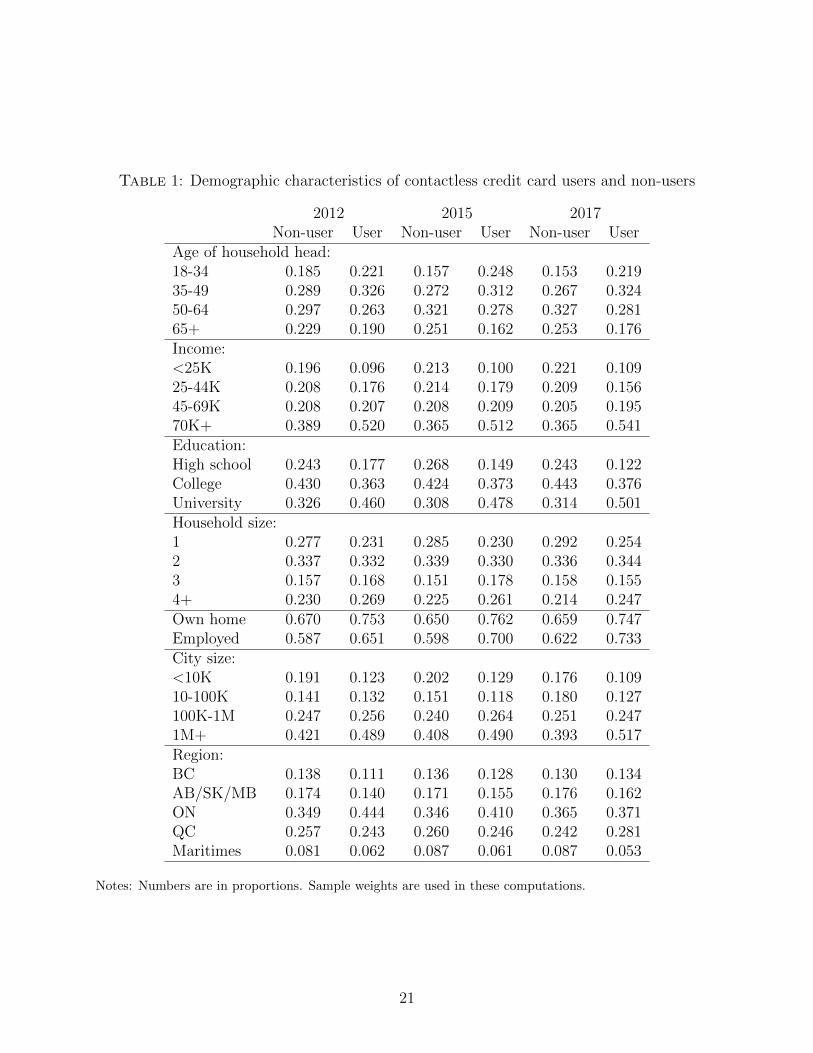
Table 1: Demographic characteristics of contactless credit card users and non-users

2012 2015 2017Non-user User Non-user User Non-user User

Age of household head:18-34 0.185 0.221 0.157 0.248 0.153 0.21935-49 0.289 0.326 0.272 0.312 0.267 0.32450-64 0.297 0.263 0.321 0.278 0.327 0.28165+ 0.229 0.190 0.251 0.162 0.253 0.176Income:<25K 0.196 0.096 0.213 0.100 0.221 0.10925-44K 0.208 0.176 0.214 0.179 0.209 0.15645-69K 0.208 0.207 0.208 0.209 0.205 0.19570K+ 0.389 0.520 0.365 0.512 0.365 0.541Education:High school 0.243 0.177 0.268 0.149 0.243 0.122College 0.430 0.363 0.424 0.373 0.443 0.376University 0.326 0.460 0.308 0.478 0.314 0.501Household size:1 0.277 0.231 0.285 0.230 0.292 0.2542 0.337 0.332 0.339 0.330 0.336 0.3443 0.157 0.168 0.151 0.178 0.158 0.1554+ 0.230 0.269 0.225 0.261 0.214 0.247Own home 0.670 0.753 0.650 0.762 0.659 0.747Employed 0.587 0.651 0.598 0.700 0.622 0.733City size:<10K 0.191 0.123 0.202 0.129 0.176 0.10910-100K 0.141 0.132 0.151 0.118 0.180 0.127100K-1M 0.247 0.256 0.240 0.264 0.251 0.2471M+ 0.421 0.489 0.408 0.490 0.393 0.517Region:BC 0.138 0.111 0.136 0.128 0.130 0.134AB/SK/MB 0.174 0.140 0.171 0.155 0.176 0.162ON 0.349 0.444 0.346 0.410 0.365 0.371QC 0.257 0.243 0.260 0.246 0.242 0.281Maritimes 0.081 0.062 0.087 0.061 0.087 0.053

Notes: Numbers are in proportions. Sample weights are used in these computations.

21

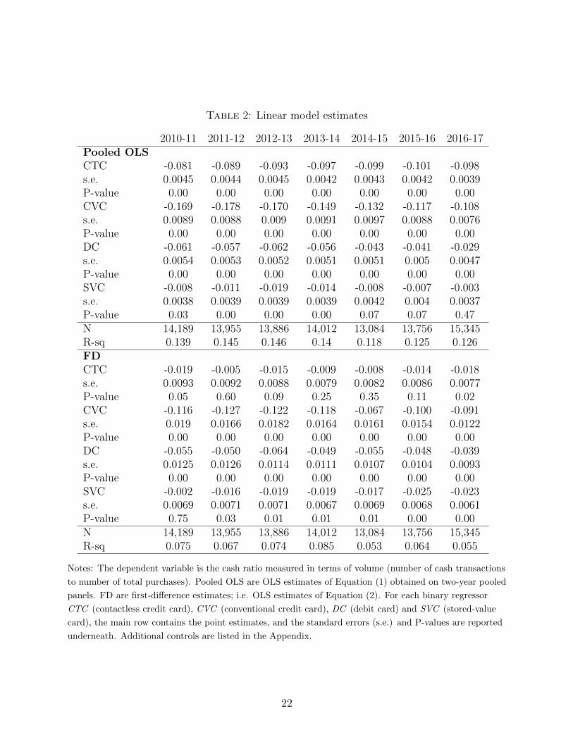
Table 2: Linear model estimates

2010-11 2011-12 2012-13 2013-14 2014-15 2015-16 2016-17Pooled OLSCTC -0.081 -0.089 -0.093 -0.097 -0.099 -0.101 -0.098s.e. 0.0045 0.0044 0.0045 0.0042 0.0043 0.0042 0.0039P-value 0.00 0.00 0.00 0.00 0.00 0.00 0.00CVC -0.169 -0.178 -0.170 -0.149 -0.132 -0.117 -0.108s.e. 0.0089 0.0088 0.009 0.0091 0.0097 0.0088 0.0076P-value 0.00 0.00 0.00 0.00 0.00 0.00 0.00DC -0.061 -0.057 -0.062 -0.056 -0.043 -0.041 -0.029s.e. 0.0054 0.0053 0.0052 0.0051 0.0051 0.005 0.0047P-value 0.00 0.00 0.00 0.00 0.00 0.00 0.00SVC -0.008 -0.011 -0.019 -0.014 -0.008 -0.007 -0.003s.e. 0.0038 0.0039 0.0039 0.0039 0.0042 0.004 0.0037P-value 0.03 0.00 0.00 0.00 0.07 0.07 0.47N 14,189 13,955 13,886 14,012 13,084 13,756 15,345R-sq 0.139 0.145 0.146 0.14 0.118 0.125 0.126FDCTC -0.019 -0.005 -0.015 -0.009 -0.008 -0.014 -0.018s.e. 0.0093 0.0092 0.0088 0.0079 0.0082 0.0086 0.0077P-value 0.05 0.60 0.09 0.25 0.35 0.11 0.02CVC -0.116 -0.127 -0.122 -0.118 -0.067 -0.100 -0.091s.e. 0.019 0.0166 0.0182 0.0164 0.0161 0.0154 0.0122P-value 0.00 0.00 0.00 0.00 0.00 0.00 0.00DC -0.055 -0.050 -0.064 -0.049 -0.055 -0.048 -0.039s.e. 0.0125 0.0126 0.0114 0.0111 0.0107 0.0104 0.0093P-value 0.00 0.00 0.00 0.00 0.00 0.00 0.00SVC -0.002 -0.016 -0.019 -0.019 -0.017 -0.025 -0.023s.e. 0.0069 0.0071 0.0071 0.0067 0.0069 0.0068 0.0061P-value 0.75 0.03 0.01 0.01 0.01 0.00 0.00N 14,189 13,955 13,886 14,012 13,084 13,756 15,345R-sq 0.075 0.067 0.074 0.085 0.053 0.064 0.055

Notes: The dependent variable is the cash ratio measured in terms of volume (number of cash transactions

to number of total purchases). Pooled OLS are OLS estimates of Equation (1) obtained on two-year pooled

panels. FD are first-difference estimates; i.e. OLS estimates of Equation (2). For each binary regressor

CTC (contactless credit card), CVC (conventional credit card), DC (debit card) and SVC (stored-value

card), the main row contains the point estimates, and the standard errors (s.e.) and P-values are reported

underneath. Additional controls are listed in the Appendix.

22

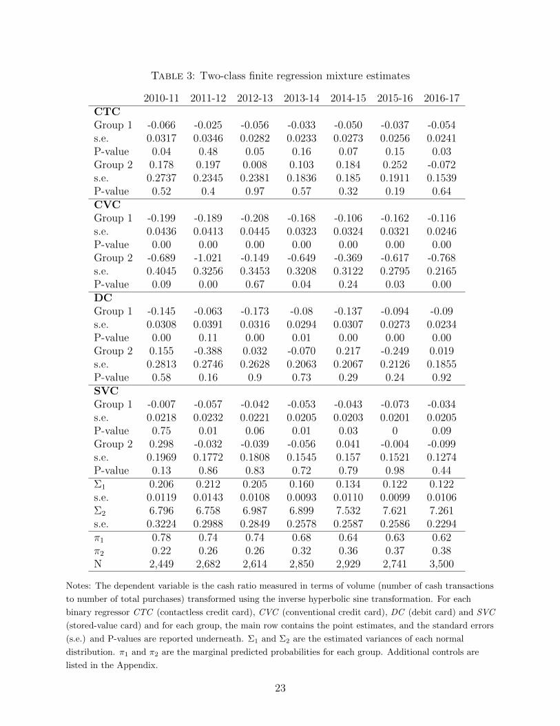
Table 3: Two-class finite regression mixture estimates

2010-11 2011-12 2012-13 2013-14 2014-15 2015-16 2016-17CTCGroup 1 -0.066 -0.025 -0.056 -0.033 -0.050 -0.037 -0.054s.e. 0.0317 0.0346 0.0282 0.0233 0.0273 0.0256 0.0241P-value 0.04 0.48 0.05 0.16 0.07 0.15 0.03Group 2 0.178 0.197 0.008 0.103 0.184 0.252 -0.072s.e. 0.2737 0.2345 0.2381 0.1836 0.185 0.1911 0.1539P-value 0.52 0.4 0.97 0.57 0.32 0.19 0.64CVCGroup 1 -0.199 -0.189 -0.208 -0.168 -0.106 -0.162 -0.116s.e. 0.0436 0.0413 0.0445 0.0323 0.0324 0.0321 0.0246P-value 0.00 0.00 0.00 0.00 0.00 0.00 0.00Group 2 -0.689 -1.021 -0.149 -0.649 -0.369 -0.617 -0.768s.e. 0.4045 0.3256 0.3453 0.3208 0.3122 0.2795 0.2165P-value 0.09 0.00 0.67 0.04 0.24 0.03 0.00DCGroup 1 -0.145 -0.063 -0.173 -0.08 -0.137 -0.094 -0.09s.e. 0.0308 0.0391 0.0316 0.0294 0.0307 0.0273 0.0234P-value 0.00 0.11 0.00 0.01 0.00 0.00 0.00Group 2 0.155 -0.388 0.032 -0.070 0.217 -0.249 0.019s.e. 0.2813 0.2746 0.2628 0.2063 0.2067 0.2126 0.1855P-value 0.58 0.16 0.9 0.73 0.29 0.24 0.92SVCGroup 1 -0.007 -0.057 -0.042 -0.053 -0.043 -0.073 -0.034s.e. 0.0218 0.0232 0.0221 0.0205 0.0203 0.0201 0.0205P-value 0.75 0.01 0.06 0.01 0.03 0 0.09Group 2 0.298 -0.032 -0.039 -0.056 0.041 -0.004 -0.099s.e. 0.1969 0.1772 0.1808 0.1545 0.157 0.1521 0.1274P-value 0.13 0.86 0.83 0.72 0.79 0.98 0.44Σ1 0.206 0.212 0.205 0.160 0.134 0.122 0.122s.e. 0.0119 0.0143 0.0108 0.0093 0.0110 0.0099 0.0106Σ2 6.796 6.758 6.987 6.899 7.532 7.621 7.261s.e. 0.3224 0.2988 0.2849 0.2578 0.2587 0.2586 0.2294π1 0.78 0.74 0.74 0.68 0.64 0.63 0.62π2 0.22 0.26 0.26 0.32 0.36 0.37 0.38N 2,449 2,682 2,614 2,850 2,929 2,741 3,500

Notes: The dependent variable is the cash ratio measured in terms of volume (number of cash transactions

to number of total purchases) transformed using the inverse hyperbolic sine transformation. For each

binary regressor CTC (contactless credit card), CVC (conventional credit card), DC (debit card) and SVC

(stored-value card) and for each group, the main row contains the point estimates, and the standard errors

(s.e.) and P-values are reported underneath. Σ1 and Σ2 are the estimated variances of each normal

distribution. π1 and π2 are the marginal predicted probabilities for each group. Additional controls are

listed in the Appendix.

23

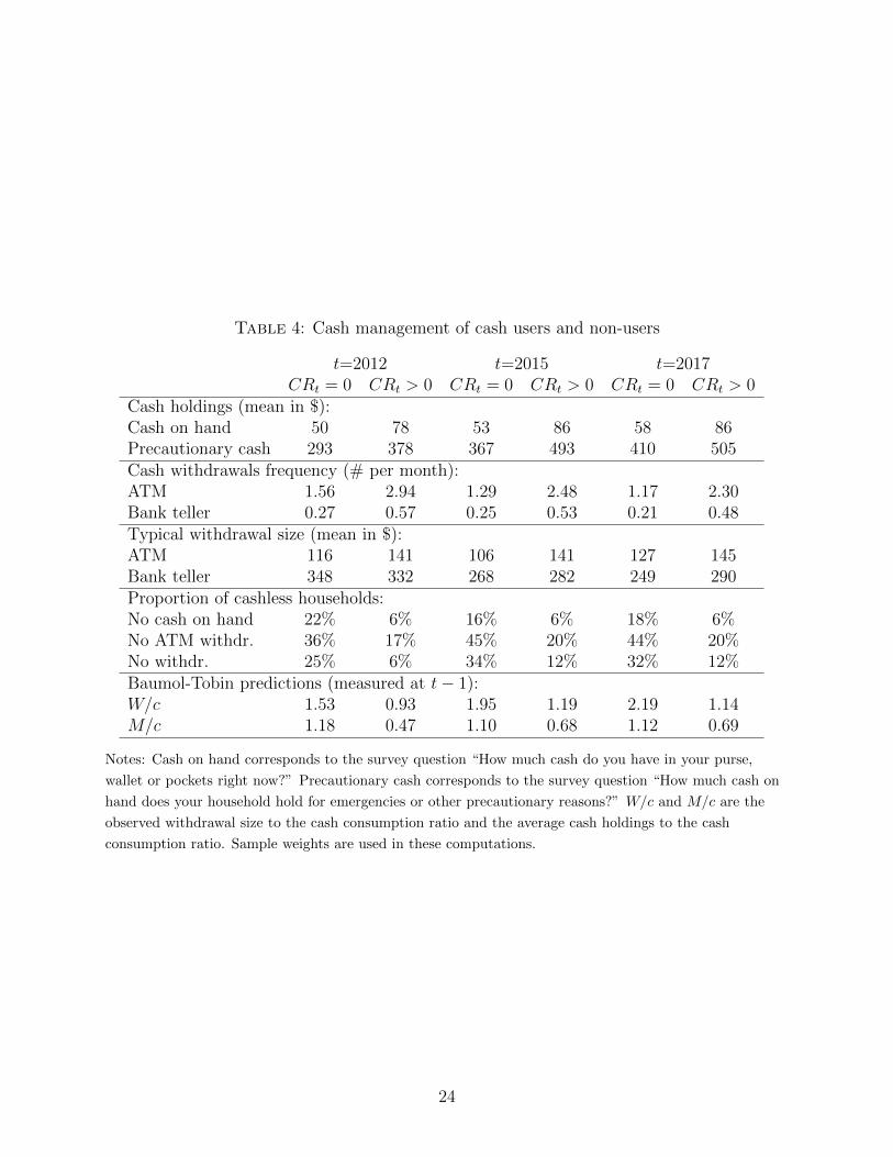
Table 4: Cash management of cash users and non-users

t=2012 t=2015 t=2017CRt = 0 CRt > 0 CRt = 0 CRt > 0 CRt = 0 CRt > 0

Cash holdings (mean in $):Cash on hand 50 78 53 86 58 86Precautionary cash 293 378 367 493 410 505Cash withdrawals frequency (# per month):ATM 1.56 2.94 1.29 2.48 1.17 2.30Bank teller 0.27 0.57 0.25 0.53 0.21 0.48Typical withdrawal size (mean in $):ATM 116 141 106 141 127 145Bank teller 348 332 268 282 249 290Proportion of cashless households:No cash on hand 22% 6% 16% 6% 18% 6%No ATM withdr. 36% 17% 45% 20% 44% 20%No withdr. 25% 6% 34% 12% 32% 12%Baumol-Tobin predictions (measured at t− 1):W/c 1.53 0.93 1.95 1.19 2.19 1.14M/c 1.18 0.47 1.10 0.68 1.12 0.69

Notes: Cash on hand corresponds to the survey question “How much cash do you have in your purse,

wallet or pockets right now?” Precautionary cash corresponds to the survey question “How much cash on

hand does your household hold for emergencies or other precautionary reasons?” W/c and M/c are the

observed withdrawal size to the cash consumption ratio and the average cash holdings to the cash

consumption ratio. Sample weights are used in these computations.

24

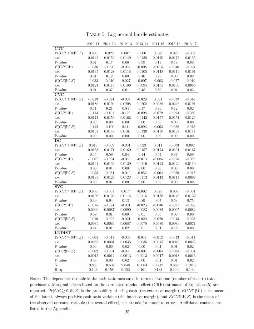
Table 5: Log-normal hurdle estimates

2010-11 2011-12 2012-13 2013-14 2014-15 2015-16 2016-17CTCPr(CR ≥ 0|W,Z) 0.000 0.020 0.007 0.000 0.026 0.023 -0.002s.e. 0.0143 0.0150 0.0149 0.0135 0.0170 0.0173 0.0155P-value 0.97 0.17 0.66 0.99 0.13 0.18 0.88E(CR∗|W ) -0.036 -0.020 -0.034 -0.008 -0.015 -0.046 -0.024s.e. 0.0135 0.0128 0.0118 0.0105 0.0118 0.0119 0.0101P-value 0.01 0.12 0.00 0.46 0.20 0.00 0.02E(CR|W,Z) -0.033 -0.010 -0.027 -0.007 -0.003 -0.027 -0.019s.e. 0.0124 0.0114 0.0109 0.0095 0.0105 0.0105 0.0086P-value 0.01 0.37 0.01 0.48 0.80 0.01 0.03CVCPr(CR ≥ 0|W,Z) -0.019 -0.024 -0.004 -0.029 0.001 -0.039 -0.046s.e. 0.0186 0.0194 0.0208 0.0208 0.0239 0.0246 0.0191P-value 0.31 0.21 0.84 0.17 0.96 0.12 0.02E(CR∗|W ) -0.114 -0.101 -0.126 -0.098 -0.079 -0.094 -0.080s.e. 0.0171 0.0150 0.0162 0.0142 0.0157 0.0151 0.0123P-value 0.00 0.00 0.00 0.00 0.00 0.00 0.00E(CR|W,Z) -0.112 -0.100 -0.114 -0.096 -0.063 -0.088 -0.078s.e. 0.0167 0.0146 0.0161 0.0139 0.0150 0.0137 0.0111P-value 0.00 0.00 0.00 0.00 0.00 0.00 0.00DCPr(CR ≥ 0|W,Z) 0.013 -0.009 -0.001 0.023 0.011 -0.003 0.002s.e. 0.0168 0.0171 0.0169 0.0157 0.0174 0.0191 0.0167P-value 0.45 0.59 0.94 0.14 0.54 0.87 0.89E(CR∗|W ) -0.067 -0.034 -0.055 -0.070 -0.085 -0.075 -0.062s.e. 0.0141 0.0136 0.0129 0.0119 0.0122 0.0129 0.0110P-value 0.00 0.01 0.00 0.00 0.00 0.00 0.00E(CR|W,Z) -0.055 -0.034 -0.049 -0.052 -0.064 -0.059 -0.047s.e. 0.0133 0.0128 0.0123 0.0113 0.0113 0.0114 0.0096P-value 0.00 0.01 0.00 0.00 0.00 0.00 0.00SVCPr(CR ≥ 0|W,Z) 0.009 -0.001 0.017 -0.002 0.025 0.009 -0.004s.e. 0.0106 0.0109 0.0115 0.0115 0.0136 0.0146 0.0132P-value 0.39 0.94 0.13 0.89 0.07 0.53 0.75E(CR∗|W ) -0.015 -0.024 -0.031 -0.023 -0.036 -0.021 -0.028s.e. 0.0090 0.0087 0.0090 0.0083 0.0085 0.0095 0.0082P-value 0.09 0.01 0.00 0.01 0.00 0.03 0.00E(CR|W,Z) -0.010 -0.022 -0.021 -0.020 -0.020 -0.013 -0.023s.e. 0.0085 0.0083 0.0087 0.0078 0.0080 0.0083 0.0071P-value 0.24 0.01 0.02 0.01 0.01 0.12 0.00LNDISTPr(CR ≥ 0|W,Z) -0.005 -0.011 -0.008 -0.011 -0.012 -0.013 -0.011s.e. 0.0032 0.0031 0.0035 0.0035 0.0045 0.0049 0.0046P-value 0.09 0.00 0.02 0.00 0.01 0.01 0.02E(CR|W,Z) -0.002 -0.004 -0.003 -0.004 -0.004 -0.005 -0.004s.e. 0.0013 0.0012 0.0013 0.0013 0.0017 0.0018 0.0016P-value 0.09 0.00 0.02 0.00 0.01 0.01 0.02N 9,885 10,534 9,848 10,684 10,442 9,688 11,813R-sq 0.143 0.158 0.152 0.161 0.133 0.140 0.144

Notes: The dependent variable is the cash ratio measured in terms of volume (number of cash to total

purchases). Marginal effects based on the correlated random effect (CRE) estimates of Equation (5) are

reported. Pr(CR ≥ 0|W,Z) is the probability of using cash (the extensive margin), E(CR∗|W ) is the mean

of the latent, always positive cash ratio variable (the intensive margin), and E(CR|W,Z) is the mean of

the observed outcome variable (the overall effect); s.e. stands for standard errors. Additional controls are

listed in the Appendix.25

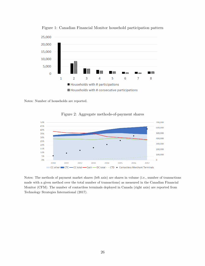
Figure 1: Canadian Financial Monitor household participation pattern

Notes: Number of households are reported.

Figure 2: Aggregate methods-of-payment shares

Notes: The methods of payment market shares (left axis) are shares in volume (i.e., number of transactions

made with a given method over the total number of transactions) as measured in the Canadian Financial

Monitor (CFM). The number of contactless terminals deployed in Canada (right axis) are reported from

Technology Strategies International (2017).

26

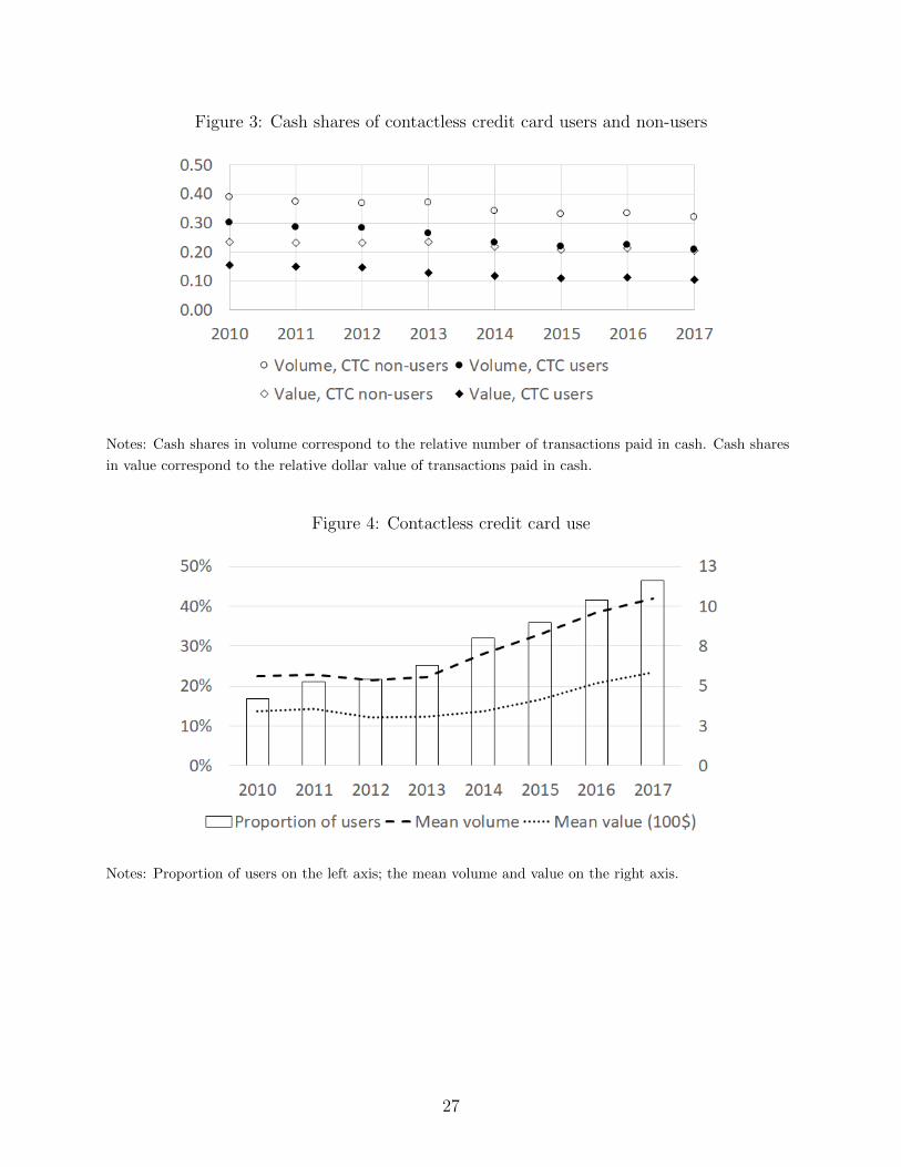
Figure 3: Cash shares of contactless credit card users and non-users

Notes: Cash shares in volume correspond to the relative number of transactions paid in cash. Cash shares

in value correspond to the relative dollar value of transactions paid in cash.

Figure 4: Contactless credit card use

Notes: Proportion of users on the left axis; the mean volume and value on the right axis.

27

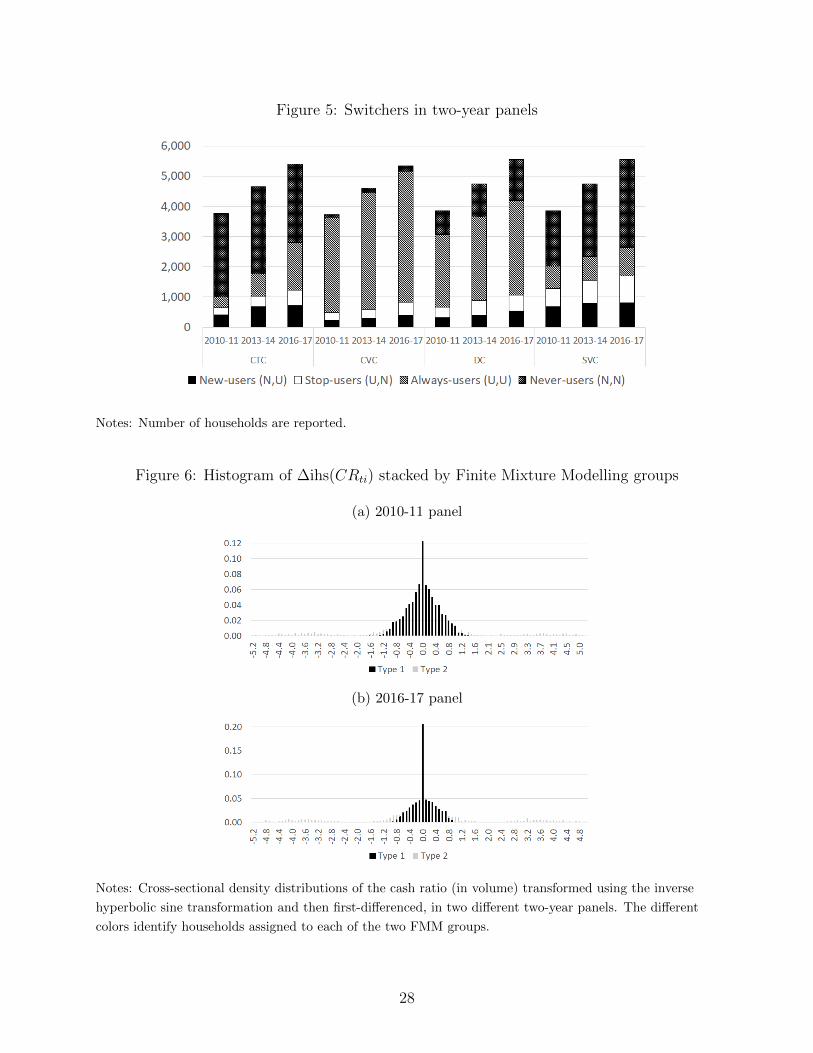
Figure 5: Switchers in two-year panels

Notes: Number of households are reported.

Figure 6: Histogram of ∆ihs(CRti) stacked by Finite Mixture Modelling groups

(a) 2010-11 panel

(b) 2016-17 panel

Notes: Cross-sectional density distributions of the cash ratio (in volume) transformed using the inverse

hyperbolic sine transformation and then first-differenced, in two different two-year panels. The different

colors identify households assigned to each of the two FMM groups.

28

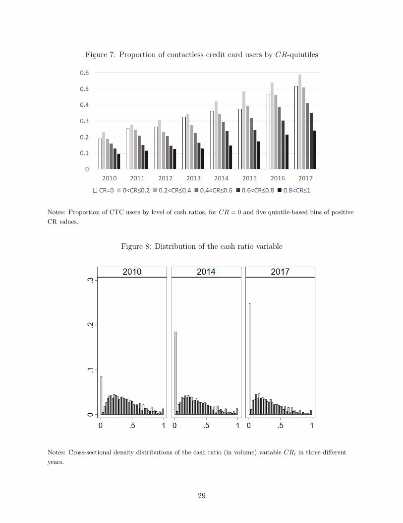
Figure 7: Proportion of contactless credit card users by CR-quintiles

Notes: Proportion of CTC users by level of cash ratios, for CR = 0 and five quintile-based bins of positive

CR values.

Figure 8: Distribution of the cash ratio variable

Notes: Cross-sectional density distributions of the cash ratio (in volume) variable CRi in three different

years.

29

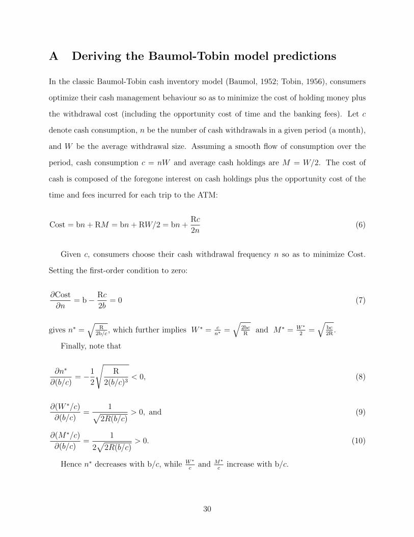
A Deriving the Baumol-Tobin model predictions

In the classic Baumol-Tobin cash inventory model (Baumol, 1952; Tobin, 1956), consumers

optimize their cash management behaviour so as to minimize the cost of holding money plus

the withdrawal cost (including the opportunity cost of time and the banking fees). Let c

denote cash consumption, n be the number of cash withdrawals in a given period (a month),

and W be the average withdrawal size. Assuming a smooth flow of consumption over the

period, cash consumption c = nW and average cash holdings are M = W/2. The cost of

cash is composed of the foregone interest on cash holdings plus the opportunity cost of the

time and fees incurred for each trip to the ATM:

Cost = bn+ RM = bn+ RW/2 = bn+Rc

2n(6)

Given c, consumers choose their cash withdrawal frequency n so as to minimize Cost.

Setting the first-order condition to zero:

∂Cost

∂n= b− Rc

2b= 0 (7)

gives n∗ =√

R2b/c

, which further implies W ∗ = cn∗ =

√2bcR

and M∗ = W ∗

2=

√bc2R

.

Finally, note that

∂n∗

∂(b/c)= −1

2

√R

2(b/c)3< 0, (8)

∂(W ∗/c)

∂(b/c)=

1√2R(b/c)

> 0, and (9)

∂(M∗/c)

∂(b/c)=

1

2√

2R(b/c)> 0. (10)

Hence n∗ decreases with b/c, while W ∗

cand M∗

cincrease with b/c.

30

B Measuring the distance to the closest bank branch

I use a measure of the distance to the closest branch developed in Chen and Strathearn (2020)

and graciously shared by the authors. Using Payments Canada’s Financial Institutions File

for the period 2008-2018, these authors first geocode all bank branches locations in Canada.

Then, they (i) create an evenly spaced fine grid of points for each forward sortation area

(FSA) (this corresponds to the first three characters of the postal code); (ii) calculate the

Haversine distance between each grid point and the nearest branch; (iii) compute the average

distance across all grid points within that FSA. This measure represents, on average, how

far an individual would need to travel to reach the closest bank branch. This measure varies

at the year and FSA level. I refer the reader to Chen and Strathearn (2020) for additional

details. For my analysis I use yearly measures for the period 2010-2017.

31

C Variables description

This section describes the variables from the Canadian Financial Monitor used in my analysis.

• Payment method indicators CTC, CVC, DC and SVC : these are dummy variables

that indicate whether any member of the household used a given payment method to

make purchases in the past month.

• CC revolver: this is a dummy variable indicating whether any member of the household

revolved their credit card balance in the past month.

• Number of credit cards in the household.

• Number of debit cards in the household.

• Internet user: a dummy variable indicating whether any member of the household uses

the Internet.

• Household income for the past year before taxes.

• Month of survey participation.

• Dummy variable indicating whether the respondent is a head of a household.

• Dummy variable indicating the gender of the respondent.

• Time in Canada: less than 10 years, over 10 years, born in Canada.

• Education level: High school or below, college, university.

• City size: less than 10K, between 10 and 100K, over 100K.

• Region: BC, AB/SK/MB, ON, QC or Maritimes.

• Attitudes: see explanations below.

• Types of expenditure: see explanations below.

32

Types of expenditure: To avoid potential endogeneity issues, household expenditures in

various categories are measured as ratios relative to the average within the individual’s de-

mographic stratum (defined according to age and income group), following Stango (2000).

Expenditure categories considered are: groceries, including beverages; food and beverages

at restaurants/clubs/bars; snacks and beverages from convenience stores; recreation; auto-

mobile maintenance/gas. For each household, I calculate the share of expenditures made in

each category in the past month relative to the total value of purchases made in the past

month.

Attitudes: Using Likert scales, the CFM collects information on attitudes of the male

and/or female heads of households toward various statements related to their financial sit-

uations or decisions. Throughout the paper, I include as controls in the regressions these

heads of households’ attitudes towards the following statements (regrouped here by theme):

• Level of indebtedness/financial situation: “I have difficulty paying off my debt”; “I

am comfortable with the amount of debt that I am carrying”; “I feel confident that I

will have enough money to retire comfortably”; “I am satisfied with my household’s

current financial situation”; “Financially, I am better off now than a year ago”; “A

year from now, I will be financially better off than I am today.”

• Risk: “I don’t like to invest in the stock market because it is too risky”; “I am willing

to take substantial risks to earn substantial returns.”

• Confidence/decision-making: “I wish I was more confident about making financial

decisions”; “I believe a financial advisor could help me in today’s economic situation”;

“I like to consult a professional investment advisor, but I make my own decisions about

my investments” (since 2013); “I am willing to pay for good financial advice”; “I like

talking to a professional when making important financial decisions.”

• Forward-lookingness/financial planning: “Being able to retire in comfort is a constant

concern for me”; “I need to work with a professional financial advisor on a financial

33

plan for the future.”

• Technology: “I prefer to deal with people when I bank” (since 2013); “There are so

many financial products and services that I sometimes find it confusing” (since 2013).

34