L4-13653

Approved forpublic release;distribution is unlimited.

Comparison among Five Hydrodynamic Codes

with a Diverging-Converging

Nozzle Experiment

Los AlamosNATIONAL LABORATORY

Los Alamos Nafional .haborafoq is operafed by fhe University of Cal~orniafor theUnited Stafes Department of &x?rgy under con fract W-7405-ENG-36.

Edited by Patricia W. Mendius, Grou~ ClC-l

An A+j%mative Action/Equal Opportunity Employer

This report was prepared as an account of work sponsored by an agency of the United StatesGovernment. Neither The Regents of the University of Cal#ornia, the United StatesGovernment nor any agency thereofi nor any of their employees, makes any warranty, expressor implied, or assumes any legal liabilify or responsibility for the accuracy, completeness,oruseyfdnessof any information, apparatus, producf, or processdisclosed,or represents fhaf ifsuse would not infringe privately owned rights. Referenceherein to any specz$ccommercialproduct, process, or service by trade name, trademark, rrcanufacfurer,or otherwise, does notnecessarily constitute or imply its endorsernent,recommendafion, orfavoring by The Regentsof the University of Calz~ornia,the Unifed Sfates Government, or any agency thereo~ Theviews and opinions of authors expressed herein do not necessarilystafe or reject thoseofThe Regenfs of fhe University of Cal~ornia, the Unifed Stafes Government, or any agencythereo$ Los A[amos National tiboratoy strongly supports academicfreedom and aresearcher’srzghf fo publish; as an irzstitufion, however, fhe Laboratorydoes nof endorse fhevieurpoinf oja publication or guaranfee its techniad correctness.

DISCLAIMER

Portions of this document may be illegiblein electronic image products. Images areproduced from the best available originaldocument.

LA-13653

Issued: September 1999

Comparison among Five Hydrodynamic Codes

with a Diverging-Converging

Nozzle Experiment

L. E. Thode

M. C. Cline

B. G, DeVolder

M. S. Sahota

D. K. Zerkle

Los AlamosNATIONAL LABORATORY

Los Alamos, New Mexico 87545

COMPARISON AMONG FIVE HYDRODYNAMIC CODES WITHA DIVERGING-CONVERGING NOZZLE EXPERIMENT

byL. E. Thode, M. C. Cline, B. G. DeVolder, M. S. Sahota, and D. K. Zerkle

Abstract

A realistic open-cycle gas-core nuclear rocket simulation model must be capable of a self-consistent nozzle calculation in conjunction with coupled radiation and neutron transportin three spatial dimensions. ‘As part of the development effort for such a model, fivehydrodynamic codes were used to compare with a converging-diverging nozzleexperiment. The codes used in the comparison are CHAD, FLUENT, KIVA2,RAMPANT, and VNAP2. Solution accuracy as a function of mesh size is importantbecause, in the near term, a practical three-dimensional simulation model will requirerather coarse zoning across the nozzle throat. In the study, four different grids wereconsidered. 1) coarse, radially uniform grid, 2) coarse, radially nonuniform grid, 3) fine,radially uniform grid, and 4) fine, radially nonuniform grid. The study involves codeverification, not prediction. In other words, we know the solution we want to match, sowe can change methods and/or modify an algorithm to best match this class of problem.In this context, it was necessary to use the higher-order methods in both FLUENT andRAMPANT. Ih addition, KIVA2 required a modification that allows significantly moreaccurate solutions for a converging-diverging nozzle. From a predictive point of view,code accuracy with no tuning is an important result. The most accurate codes on a coarsegrid, CHAD and VNAP2, did not require any tuning. Our main comparison among thecodes was the radial dependence of the Mach number across the nozzle throat. All fivecodes yielded a very similar solution with fine, radially uniform and radially nonuniformgrids, However, the codes yielded significantly different solutions with coarse, radiallyuniform and radially nonuniform grids. For all the codes, radially nonuniform zoningacross the throat significantly increased solution accuracy with a coarse mesh. None ofthe codes agrees in detail with the weak shock located downstream of the nozzle throat,but all the codes indicated the presence of a weak downstream shock.

-1-

Introduction

The concept of an open-cycle gas-core nuclear rocket (OCGCNR) was studied

extensively during the 1970s. 1>2Although many small-scale experiments were reported, a

self-consistent computational treatment of the engine was not possible. More recently, a

computational model for the OCGCNR was reported by Poston-Kammash (PK).3

Although the PK model couples hydrodynamics with radiation diffusion and neutron

transport, the model assumes an axisymmetric geometry. Moreover, the PK model does

not treat the engine nozzle in a self-consistent fashion, which appears to lead to a

sensitive dependence of the uranium plasma confinement upon rocket acceleration.

With the advent of large-scale massively parallel computers, a realistic OCGCNR

simulation appears possible. Given this capability, a scoping study

determine the requirements for a comprehensive OCGCNR model!

was performed to

From the scoping

study, a realistic OCGCNR model must be capable of a self-consistent nozzle calculation

in conjunction with coupled radiation transport and neutron transport in three spatial

dimensions. The importance of a self-consistent nozzle calculation leads to the issue of

hydrodynamic algorithm accuracy for a converging-diverging nozzle. In particular,

solution accuracy as a function of the mesh size is important because a practical

OCGCNR calculation will require rather coarse zoning across the nozzle throat.

A converging-diverging nozzle is an important problem with much broader

interest than just OCGCNR model development. So, a few validation calculations turned

into a modest comparison study of five hydrodynamic codes with an experiment. A

converging-diverging nozzle flow offers a rigorous test of computational fluid dynamic

methods because of the significant regions of subsonic, transonic, and supersonic flow. In

-2-

addition, the flow in the throat region exhibits large gradients due to the large wall

curvature and transonic speed. The experiment selected for this study is the converging-

diverging nozzle investigated by Cuffel et aL5 Previously, the experiment was calculated

by Prozan (as reported by Cuffel et al.5 and Saunders), Migdal et aL,7 LavaI,* Serra,9 and

Cline10 using time-dependent methods, and by Prozan and Kookerl 1 using a relaxation

procedure. A survey of nozzle methods can be found in Reference 12.

Summary of Hydrodynamic Codes

The codes CHAD,’3 FLUENT,14 KIVA2,’5 RAMPANT,14 and VNAP216 all differ

at a fundamental algorithm level. Moreover, the codes differ significwtly in their

approach to setup, execution, and solution analysis.

CHAD

CHAD13 solves the three-dimensional, time-dependent, compressible Navier-

Stokes equations for a turbulent, multimaterial fluid at all flow speeds employing an

unstructured mesh on massively parallel computing platforms. The turbulence calculation

uses a k-& model. CHAD is based on a node-centered, finite-volume method in which all

fluid variables are located at computational nodes. CHAD utilizes a variable

explicit/implicit upwind method for convection that improves computational efficiency in

flows that have large velocity Courant number variations due to velocity or mesh size

variations. Strong shocks are handled through the use of a tensor form for the artificial

viscosity.

FLUENT

FLUENT is

dimensional coupled

a product of Fluent Incorporated. 14 The code solves the three-

equations for mass, momentum, energy, and chemical species using

-3-

a control volume based finite-difference scheme with the SIMPLE algorithm (Semi-

Implicit Method for Pressure-Linked Equations). To facilitate calculations on complex

geometry, the equations are discretized on a curvilinear grid. We employed the four-level

multigrid convergence accelerator option. In this study, a cylindrical coordinate system

was used. The code has a large number of options that can be selected by the user for the

interpolation and solution methods. Finally, FLUENT offers a steady-state option, which

we used to obtain an initial guess for the time-dependent calculations. In all cases, the

steady-state and time-dependent solutions were essentially the same.

KIVA2

The KIVA215 code solves the three-dimensional, time-dependent, compressible

Navier-Stokes equations for the motion of a turbulent, chemically reactive mixture of

ideal gases, coupled to the equations for a single-component vaporizing fuel spray. The

gas-phase solution procedure is based on the ALE (Arbitrary Lagrangian Eulerian) finite-

volume method. The arbitrary structured mesh can conform to curved boundaries. The

diffhsion terms as well as the terms associated with pressure wave propagation are

difference implicitly using a method similar to the SIMPLE algorithm. The convection

terms are difference using an explicit quasi-second-order upwind scheme that is

subcycled.

RAMPANT

RAMPANT is a product of Fluent Incorporated.14 The code solves the coupled

three-dimensional equations for mass, momentum, and energy in complex geometry using

a finite-volume scheme on an unstructured mesh. We employed the four-level multigrid

convergence accelerator option. As in FLUENT, there are a large number of options that

-4-

can be selected by the user for the interpolation and solution methods. Again, as in

FLUENT, RAMPANT offers a steady-state option, which we used to obtain an initial

guess for the time-dependent calculations. In all cases, the steady-state and time-

dependent solutions were essentially the same.

VNAP2

The VNAP216 code solves the two-dimensional, time-dependent, compressible

Navier-Stokes equations for the motion of a turbulent, ideal gas. Problems can be solved

in either a Cartesian or a cylindrical coordinate system. The grid is nonuniform with

body-fitted coordinates in one direction. The unsplit, explicit MacCormack scheme is

used to solve the finite-difference equations in the interior of the mesh and a reference-

plane characteristic scheme is employed at the boundaries. Artificial viscosity can be used

to control algorithm stability.

Code Options

The study is one of code verification, not prediction. In other words, we know the

solution we are attempting to match, so we can change methods and/or modify an

algorithm to best match this class of problem. Jn this context, several different code

options were considered for both FLUENT and KIVA2. A summary of the different code

options is listed in Table I.

In Table I, CHAD denotes the standard code which is fully implicit with in

internal time step calculation. In all cases, the code was run with the Eulerian option.

Three FLUENT options were considered. The Graphics User Interface (GUI) path

for the three options is given in Table I. The options reflect differences in the order of the

discretization scheme associated with the mass, momentum, and energy equations as well

-5-

as in the interpolation scheme. In all cases, we were able to reduce the residuals by about

six orders-of-magnitude in the steady-state mode. So, the differences among the options

are not due to different levels of convergence, rather they reflect the differences in the

algorithms. In option FLUENT-1, the higher-order schemes are turned off and the

“power-law” interpolation scheme is used. In option FLUENT-2, the higher-order

schemes are turned on and the “2nd order upwind” option is used. In option FLUENT-3,

the higher-order schemes are turned on and the “quick” (quadratic interpolation) option is

used.

We considered four options for KIVA2. In Table I, the option KIVA2-1 denotes

the standard code using the internally calculated time step. This time step results in at

least fifteen explicit subcycles of the convection terms, resulting in a

coupled solution. The option KIVA2-2 denotes the standard code using the

less accurate

same explicit

time step employed in the VNAP2 calculation, a time step that is significantly smaller

than the time step calculated internally by KIVA2. As a result, the solution accuracy was

greatly improved with only three explicit subcycles of the convection terms required.

Finally, the cases KIVA2-3 and IUVA2-4 denote the internally calculated and explicit

WAP2 time steps, respectively, but with a modified version of KIVA2. The code

modification consisted of changing the coefficients of the DUAL, DUAF, and DUAB

terms in subroutine UFINIT from 0.125 to 0.250. This modified value was actually in the

original version of KIVA2, but the coefficient was changed to 0.125 in later versions of

the code.

Based upon the FLUENT results, RAMPANT was only run with a higher-order

scheme. The basic GUI path for the higher-order option is given in Table I. In all cases,

-6-

the RAMPANT solutions were solved with second-order spatial discretization of the

conservation equations (finite-volume scheme) ‘ind an explicit multi-stage Runge-Kutta

time integrator.

The VNAP2 code performed the coarse-uniform and coarse-nonuniform mesh

solutions without any explicit artificial viscosity. However, the truncation error

smoothing inherent to the method was so small on the fine,

radially nonuniform meshes that a small amount of artificial

radially uniform and. fine,

viscosity was required for

algorithm stability.

Flow Model, Initial Conditions, and Boundary Conditions

The fluid-flow model was assumed to be two-dimensional, axisymmetric, and

inviscid.

For the time-dependent codes CHAD, KIVA2, and VNAP2, the initial conditions

consisted of one-dimensional, isentropic, variable-area flow. The two velocity

components were adjusted so that the velocity magnitude remained constant at the one-

dimensionaI value and the local flow direction was tangent to the nozzle wall and

centerline. Between the wall and centerline, the local flow direction varied linearly. For

the time-dependent options with FLUENT and RAMPANT, the initial conditions were

obtained from the steady-state options.

For CHAD, KIVA2, and VNAP2, the inlet boundary conditions were the

specification of static pressure, density, and flow direction. The one-dimensional values

were used for the pressure and density while the inlet flow direction was assumed to be

parallel to the centerline. For FLUENT and RAMPANT, the inlet boundary conditions

-7-

were stagnation pressure, stagnation temperature, and inlet flow direction. Because the

initial conditions at the exit were supersonic, the various procedures used by the five

codes should have little effect on the results. The outer wall was a free-slip

condition for velocity and an adiabatic boundary condition for energy transfer.

Computational Mesh

boundary

A stringent test for algorithm accuracy is to compare the code solutions

number of different meshes. For such a comparison to be meaningful, each code

on a

must

solve the same problem on the same mesh. Thus, even though CHAD and RAMPANT

are unstructured mesh codes, we used a structured, nonuniform mesh with body-fitted

coordinates in the radial direction for all the calculations. For the study, VNAP2 was

modified to generate a grid file for CHAD, FLUENT and RAMPANT, and KIVA2.

For the comparison among the five codes we investigated four different grids.

These four grids are summarized in Table II. The first column indicates if the mesh is

coarse or fine and radially uniform or radially nonuniform. Column 2 gives the number of

axial and radial cells for each mesh. At the throat, the minimum radial zone, which occurs

at the nozzle wall, and the maximum radial zone, which occurs at the nozzle centerline,

are indicated in columns 3 and 4.

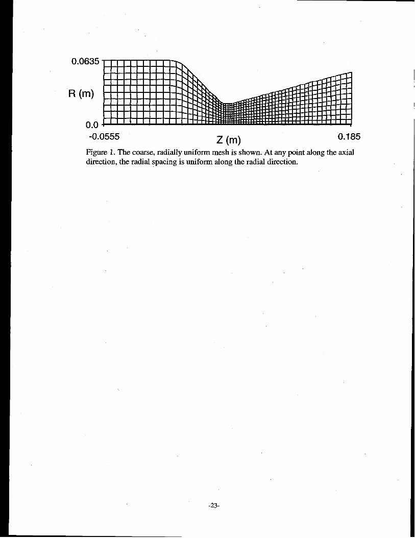
The coarse, radially uniform mesh was 61 axial cells by 10 radial cells. At any

point along the axial direction, the radial spacing is uniform along the radial direction.

But the uniform radial spacing varies with axial position in one-to-one correspondence

with the nozzle wall. Along the axial direction, the axial spacing was adjusted to maintain

approximately square cells throughout the entire computational regime. As an example,

the coarse, radially uniform mesh is shown in Fig. 1.

-8-

The coarse, radially nonuniform mesh also was 61 axial cells by 10 radial cells

with the same axial spacing as the coarse, radially uniform mesh. At each axial position,

the radial spacing was stretched to produce a cell at the nozzle wall about one-fourth that

of the coarse, radially uniform mesh. Since the number of cells was the same, the radial

spacing on the centerline was then about twice the coarse, radially uniform mesh.

The fine, radially uniform mesh was 244 axial cells by 40 radial ceils, making the

fine-mesh cell size about one-fourth the coarse-mesh cell size. Again, along the axial

direction, the axial spacing was adjusted to maintain approximately square cells

throughout the computational regime.

The fine, radially nonuniform mesh also was 244 axial cells by 40 radial cells with

the same axial spacing as the fine, radially uniform mesh. At each axial position, the

radial spacing was stretched to produce a cell at the nozzle wall about one-fourth of the

fine, radially uniform mesh. Again, because the number of cells was fried, this produced

radial spacing on the centerline that was about twice that of the fine, radially uniform

mesh.

Code-Experiment Error Estimate

Although it is possible to pick out trends from a visual comparison of the code

solutions with the experimental data, it is often quite difficult to determine the most

accurate solution. To provide a more definitive statement about solution accuracy, we

need some reference to make the comparisons. Since the experimental data are fixed, we

will use those data as a common reference. Then, our main comparison among the codes

is the Mach number as a function of radius at the nozzle throat. In particular, we calculate

the average error for each code as

“-9-

100 N lM;de-MTIaverage error(%) = ~ ~

z–1 MT ‘

where M,?xpis the experimental Mach number, h4,C0~eis the code Mach number, and N is

the number of experimental points.

One would expect, barring a fundamental implementation or setup error, that the

algorithms associated with all five codes would converge to the same solution for a

sufficiently fine mesh. Using this metric, all the codes did provide solutions that are quite

close on the fine, radially nonuniform mesh, the average difference between the solutions

being less than 0.5%.

Comparison Among Codes and Experiment

For an OCGCNR model, our main interest was code accuracy on a coarse mesh.

In three dimensions a fiie mesh calculation is not very practical, as the problem becomes

too large for scoping and/or prototype design calculations. Furthermore, with a coarse

mesh it is possible to calculate the coupled hydrodynamics, radiation transport, and

neutron transport on a common grid. As a result, there are more comparison calculations

with a coarse mesh than with a fine mesh.

In all cases, it should be understood that the mesh descriptor uniform

(nonuniform) means that the mesh is radially uniform (radially nonuniform) with the

radial spacing changing in one-to-one correspondence with the nozzle wall. In addition,

the axial spacing is adjusted to maintain approximately square cells throughout the

computational regime. For all the comparisons, the axial location is at the nozzle throat.

In the figures, the solid line represents the most accurate code solution and solid circles

-1o-

represent the experimental data. Finally, if we define r as the radial coordinate at the

throat and R as the throat radius, the dimensionless radius is r/R.

Coarse Uniform Mesh

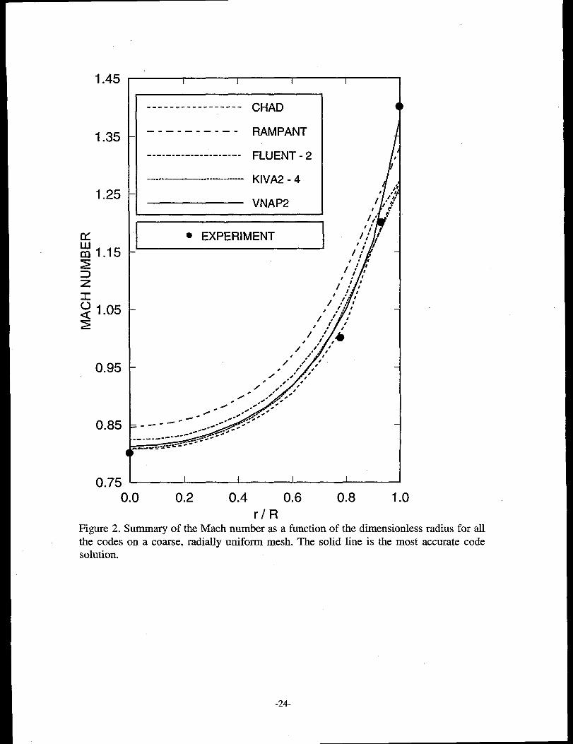
For the coarse uniform mesh, a summary of the Mach number as a function of the

dimensionless radius is shown in Fig. 2. Only the most accurate results from FLUENT

the most accurate solution

for all the code options are

and KIVA2 are included in Fig 2. The different options for FLUENT and KIVA2 are

summarized in Table I. In this case, the solid line represents

obtained from all the codes. The corresponding average errors

shown in Fig. 3.

With the coarse uniform mesh, VNAP2 provided the

seen in both Fig. 2 and Fig. 3. Except at the wall, both the FLUENT and RAMPANT

solutions are systematically high relative to the experimental data. Except at the wall,

most accurate solution, as

both CHAD and KIVA2 actually provided a more accurate solution than VNAP2. At the

wall, however, all the codes except VNAP2 provided a relatively poor solution relative to

the intefior experimental data points. With a coarse mesh, VNAP2 was expected to

provide a better wall solution because the code utilizes a special algorithm at the wall.

Because of this superior accuracy at the wall and despite the fact that CHAD and KIVA2

provided a more accurate solution at the interior points, VNAP2 provided the most

accurate solution for the entire Mach number profile. In other words, the VNAP2 solution

at the interior points was reasonable whereas the solution on the wall was much better

than dl the other codes.

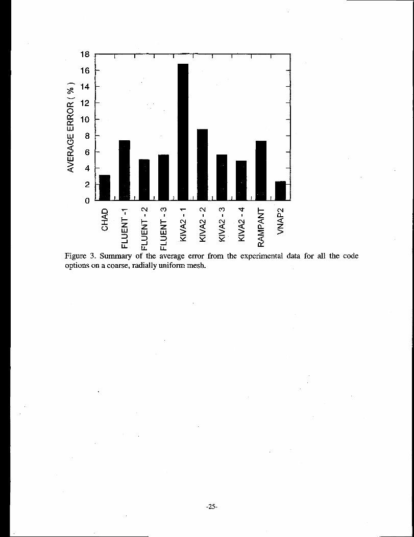
For the coarse uniform mesh there is significant variation among the different

code options, see Fig. 3. As expected, without some care one can obtain a rather poor

-11-

solution on a coarse mesh. Unless a large number of scoping calculations is done,

typically one would not compute on such a coarse mesh. However, the level of variation

among the code options was somewhat larger than we had expected. For the coarse

uniform mesh, VNAP2 provided the most accurate solution, followed by CHAD, KIVA2-

4, FLUENT-2, and RAMPANT.

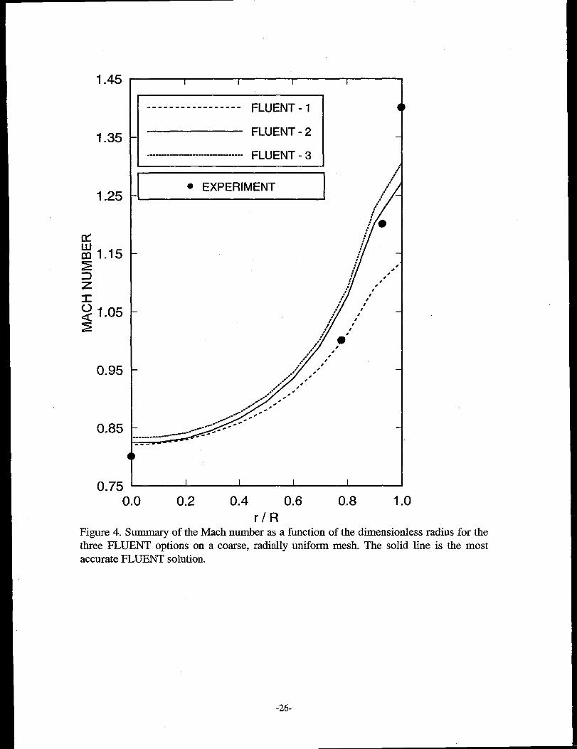
For the coarse uniform mesh, a summary of the Mach number as a function of the

dimerisionless radius for the three FLUENT options is shown in Fig. 4. In this figure, the

solid line is the most accurate FLUENT solution. All three options of the code provide a

relatively poor solution at the wall. The lowest order method appears to be especially

poor in the regions where the gradient of the Mach number with respect to radius is large.

In this respect, the higher-order interpolation options provide a significant improvement

over the lowest-order method.

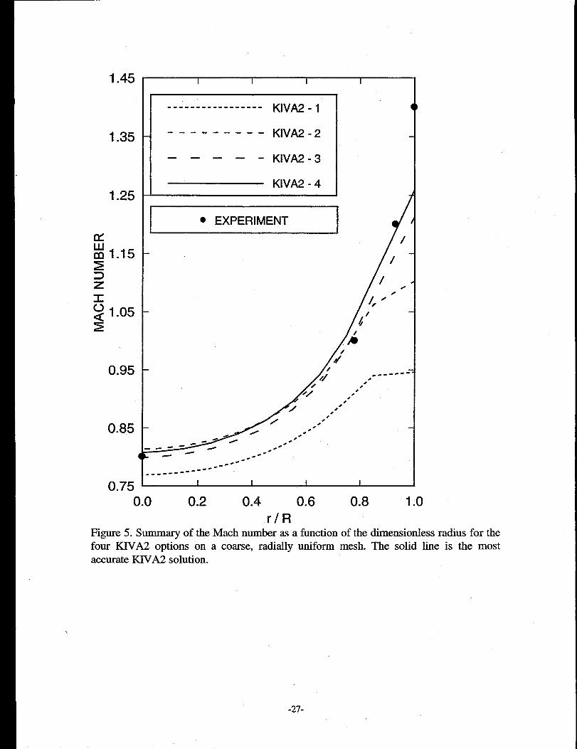
For the coarse uniform mesh, a summary of the Mach number as a function of the

dimensionless radius for the four KIVA2 options is shown in Fig. 5. In this figure, the

solid line is the most accurate KIVA2 solution. All four KIVA2 options provide a

relatively poor solution on the wall. Surprisingly, the least accurate solution is provided

by the standard KIVA2 version, which is the option KIVA2-1 in Table I. The impact of

the coefficient change is most significant when the hydrodynamic time-step is internally

calculated: compare the pairs KIVA2- 1 with KIVA2-3 and KIVA2-2 with KIVA2-4.

Basically, the. KIVA2-4 option was the only option that gave a reasonable solution. As a

result only the KIVA2-4 option was used in the remainder of the study.

-12-

Coarse Nonuniform Mesh

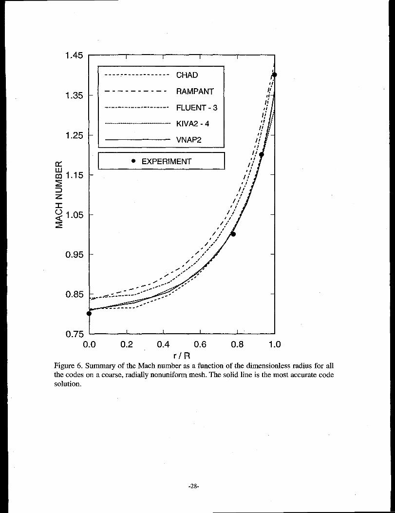
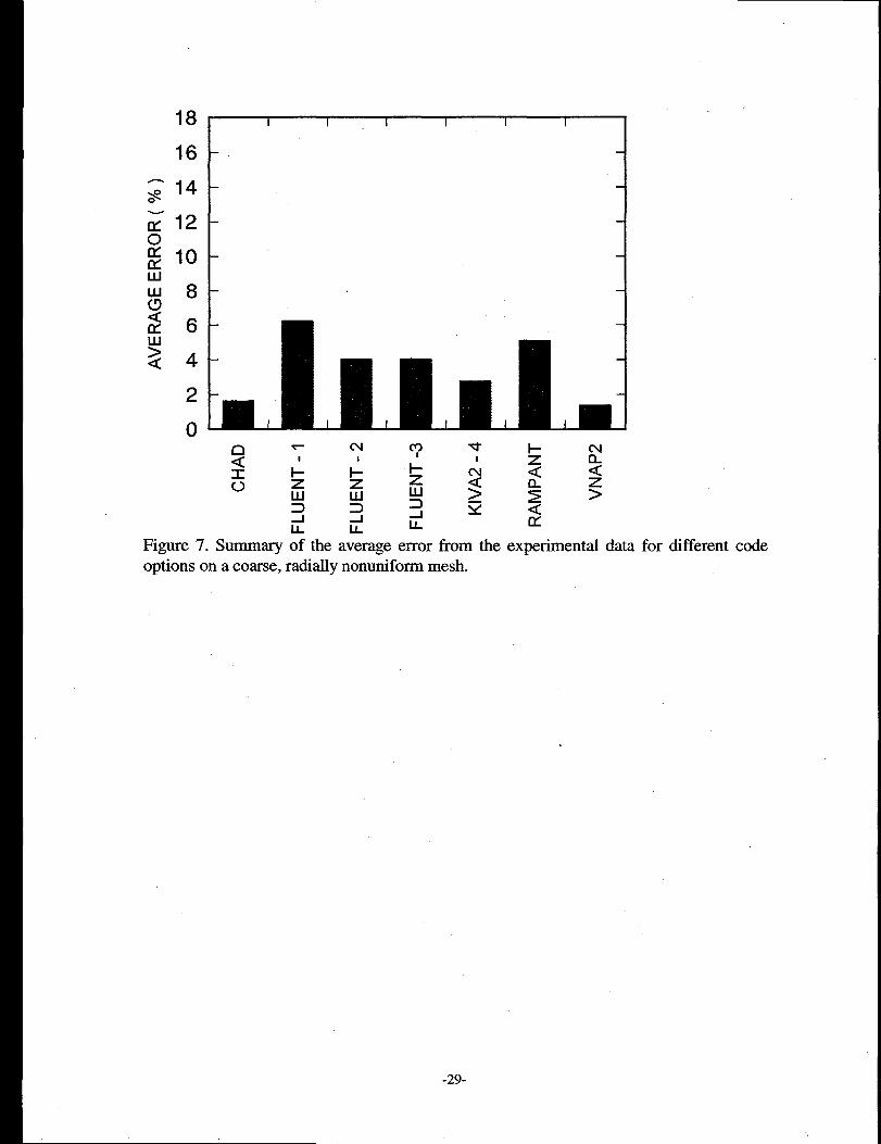
For the coarse nonuniform mesh, a summary of the Mach number as a function of

the dimensionless radius for all the codes is shown in Fig. 6. Only the most accurate

solution from FLUENT is shown in Fig. 6. The corresponding errors for all the codes and

some of the code options are shown in Fig. 7.

Consistent with the coarse uniform mesh results, Fig. 7 shows that VNAP2 again

provided the most accurate solution on the coarse nonuniform mesh. Except at the wall,

the FLUENT and ~PANT solutions remain systematically high relative to the

experimental data. For these two codes, the utilization of a nonuniform mesh provided a

mixed result at the interior points. The RAMPANT solution is slightly improved but the

FLUENT solution is somewhat worse. Furthermore, in contrast to the uniform mesh,

where the FLUENT-2 option provided the best overall solution, on the nonuniform mesh

the FLUENT-3 option

however, the difference

provided the least

between these two

average error solution. As seen in Fig. 7,

FLUENT options is insignificant. Except at

the wall, CHAD, KIVA2-4, and VNAP2 are now in close agreement with one another

and with the experimental data. For these three codes, the utilization of a nonuniform

mesh significantly improved the agreement with the interior experimental data, as can be

seen by comparing Fig. 2 with Fig. 6.

Despite these changes at the interior points, the real difference between the

uniform and nonuniform meshes occurred at the wall. With the nonuniform mesh, all the

code solutions showed a significant improvement with respect to the experimental data at

the wall. The RAMPANT solution is actually above the

the other solutions remain below the experimental data.

experimental data, whereas all

Given this trend, the observed

-13-

improvement in the average error is attributed mostly to the improved wall solution, as

can be seen by comparing Fig. 2 and Fig. 6.

Despite an improvement in the average error, Fig. 7 indicates that there still

remains a significant difference among the solutions on the coarse nonuniform mesh. For

the coarse nonuniform mesh, VNAP2 provided the most accurate solution, followed by

CHAD, KIVA2-4, FLUENT-3, and RAMPANT. Except for the change from FLUENT-2

to FHIENT-3, this code order is the same as the coarse, uniform mesh.

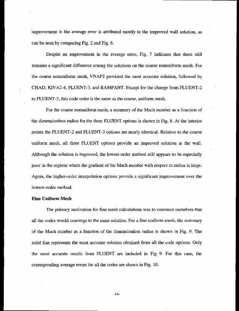
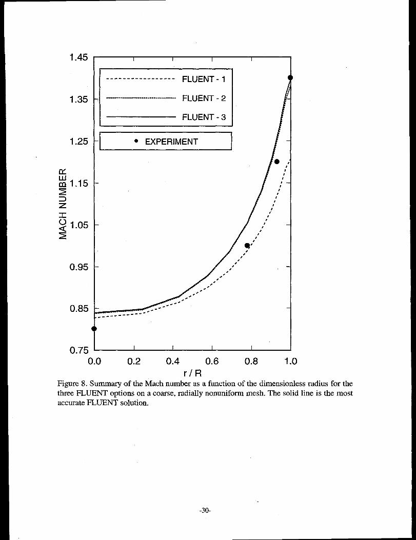
For the coarse nonuniform mesh, a summary of the Mach number as a function of

the dimensionless radius for the three FLUENT options is shown in Fig. 8. At the interior

points the FLUENT-2 and FLUENT-3 options are nearly identical. Relative to the coarse

uniform mesh, all three FLUENT options provide an improved solution at the wall.

Although the solution is improved, the lowest-order method still appears to be especially

poor in the regions where the gradient of the Mach number with respect to radius is large.

Again, the higher-order interpolation options provide a significant improvement over the

lowest-order method.

Fine Uniform Mesh

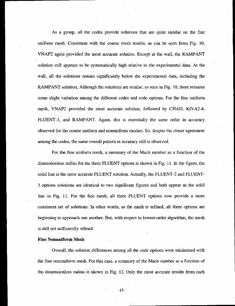
The primary motivation for fine mesh calculations was to convince ourselves that

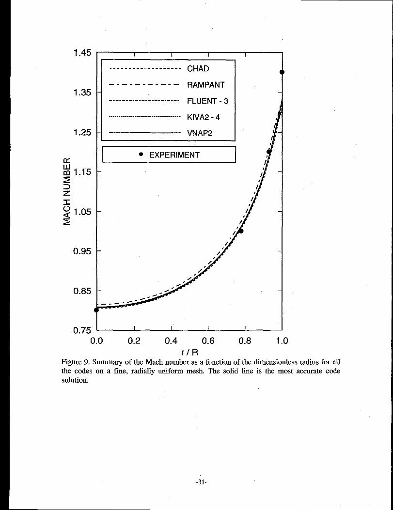
all the codes would converge to the same solution. For a fine uniform mesh, the summary

of the Mach number as a function of the dimensionless radius is shown in Fig. 9. The

solid line represents the most accurate solution obtained from all the code options. Only

the most accurate results from FLUENT are included in Fig 9. For this case, the

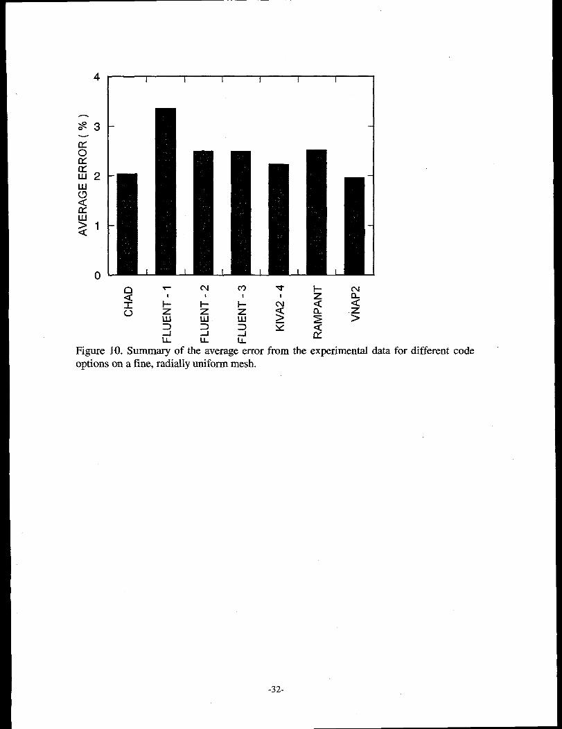
corresponding average errors for aIl the codes are shown in Fig. 10.

-14-

As a group, all the codes provide solutions that are quite similar on the fine

uniform mesh. Consistent with the coarse mesh results, as can be seen from Fig. 10,

VNAP2 again provided the most accurate solution. Except at the wall, the RAMPANT

solution still appears to be systematically high relative to the experimental data. At the

wall, all the solutions remain significantly below the experimental data, including the

RAMPANT solution. Although the solutions are similar, as seen in Fig. 10, there remains

some slight variation among the different codes and code options. For the fine uniform

mesh, VNAP2 provided the most accurate solution, followed by CHAD, KIVA2-4,

FLUENT-3, and RAMPANT. Again, this is essentially the same order in accuracy

observed for the coarse uniform and nonuniform meshes. So, despite the closer agreement

among the codes, the same overall pattern in accuracy still is observed.

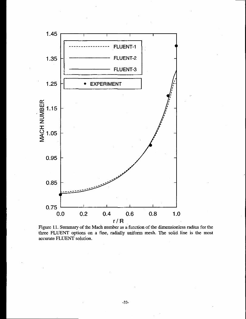
For the fine uniform mesh, a summary of the Mach number as a function of the

dimensionless radius for the three FLUENT options is shown in Fig. 11. In the figure, the

solid line is the most accurate FLUENT solution. Actually, the FLUENT-2 and FLUENT-

3 options solutions are identical to two significant figures and both appear as the solid

line in Fig. 11. For the fine mesh, all three FLUENT options now provide a more

consistent set of solutions. In other words, as the mesh is refined, all three options are

beginning to approach one another. But, with respect to lowest-order algorithm, the mesh

is still not sufficiently refined.

Fine Nonuniform Mesh

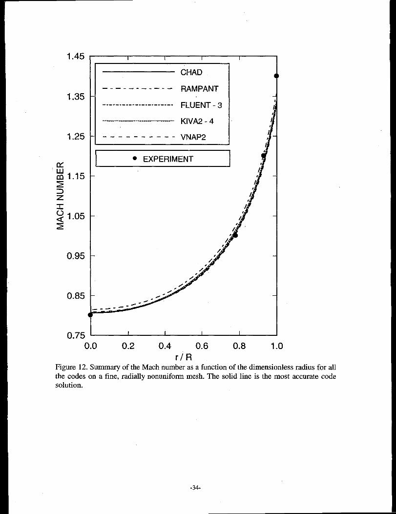
Overall, the solution differences among all the code options were minimized with

the fine nonuniform mesh. For this case, a summary of the Mach number as a function of

the dimensionless radius is shown in Fig. 12. Only the most accurate results from each

-15-

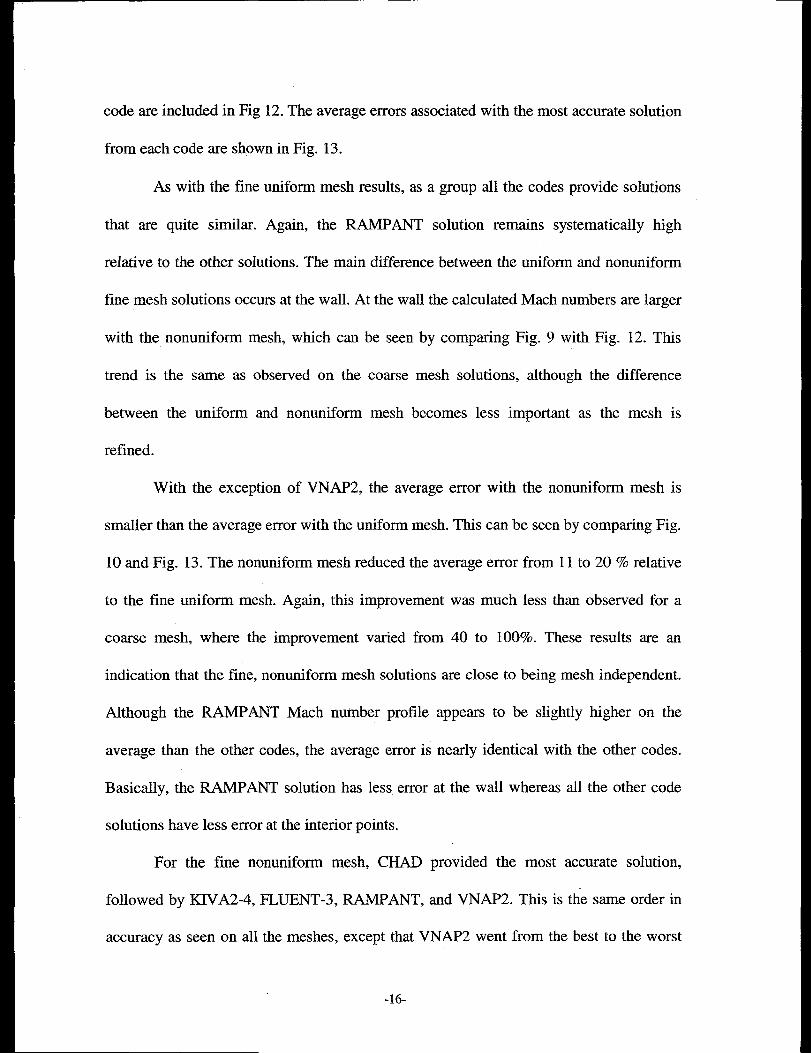
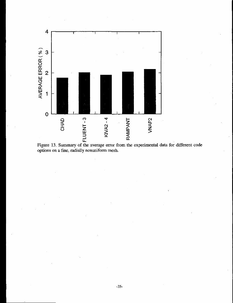
code are included in Fig 12. The average errors associated with the most accurate solution

from each code are shown in Fig. 13.

As with the fine uniform mesh results, as a group all the codes provide solutions

that are quite similar. Again, the RAMPANT solution remains systematically high

relative to the other solutions. The main difference between the uniform and nonuniform

fine mesh solutions occurs at the wall. At the wall the calculated Mach numbers are larger

with the nonuniform mesh, which can be seen by comparing Fig. 9 with Fig. 12. This

trend is the same as

between the uniform

refined.

observed on the coarse mesh solutions, although the difference

and nonuniform mesh becomes less important as the mesh is

With the exception of VNAP2, the average error with the nonuniform mesh is

smaller than the average error with the uniform mesh. This can be seen by comparing Fig.

10 and Fig. 13. The nonuniform mesh reduced the average error from 11 to 20 % relative

to the fine uniform mesh. Again, this improvement was much less than observed for a

coarse mesh, where the improvement varied from 40 to 100%. These results are an

indication that the fine, nonuniform mesh solutions are close to being mesh independent.

Although the RAMPANT Mach number profile appears to be slightly higher on the

average than the other codes, the average error is nearly identical with the other codes.

Basically, the RAMPANT solution has less error at the wall whereas all the other code

solutions have less error at the interior points.

For the fine nonuniform mesh, CHAD

followed by KIVA2-4, FLUENT-3, RAMPANT,

provided the most accurate solution,

and VNAP2. This is the same order in

accuracy as seen on all the meshes, except that VNAP2 went from the best to the worst

-16-

solution. At this point, however, the differences among the average errors have dropped

to less than 0.5%.

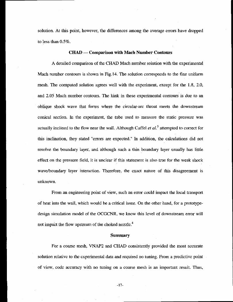
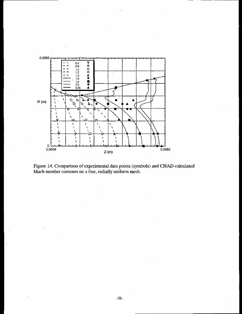
CHAD — Comparison with Mach Number Contours

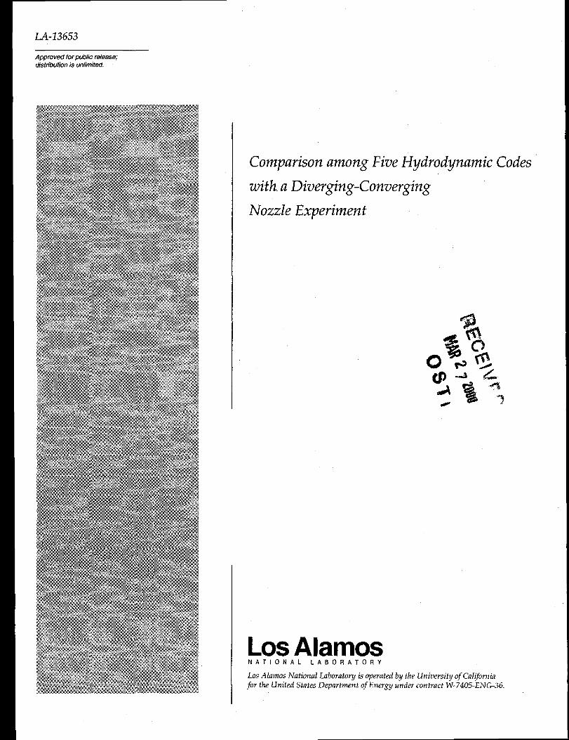
A detailed comparison of the CHAD Mach number solution with the experimental

Mach number contours is shown in Fig. 14. The solution corresponds to the fine ‘uniform

mesh. The computed solution agrees well with the experiment, except for the 1.8, 2.0,

and 2.05 Mach number contours. The kink in these experimental contours is due to an

oblique shock wave that forms where the circular-arc throat meets the downstream

conical section. In the experiment, the tube used to measure the static pressure was

actually inclined to the flow near the wall. Although Cuffel et aL5 attempted to correct for

this inclination, they stated “errors are expected.” In addition, the calculations did not

resolve the boundary layer, and although such a thin boundary layer usually has little

effect on the pressure field, it is unclear if this statement is also true for the weak shock

wave/boundary layer interaction. Therefore, the exact nature of this disagreement is

unknown.

From an engineering point of view, such an error could impact the local transport

of heat into the wall, which would be a critical issue. On the other hand, for a prototype-

design simulation model of the OCGCNR, we know this level of downstream error will

not impact the flow upstream of the choked nozzle.4

Summary

For a coarse mesh, VNAP2 and CHAD consistently provided the most accurate

solution relative to the experimental data and required no tuning.

of view, code accuracy with no tuning on a coarse mesh is an

From a predictive point

important result. Thus,

-17-

CHAD and VNAP2 can be expected to provide accurate solutions for a converging-

diverging nozzle. On the downside, however, both CHAD and VNAP2 are time-

dependent codes and are computationally intensive. In this respect, FLUENT and

RAMPANT were highly superior in computational efficiency because of a steady-state

option. However, the higher-order methods were required to obtain reasonable solution

accuracy. With the higher-order methods and a fine, radially nonuniform mesh, both the

FLUENT and RAMPANT solutions were as accurate as the CHAD and VNAP2

solutions. Finally, from a predictive point of view, one should be cautious with KIVA2

because of the required algorithm tuning needed to match the experimental data.

The solutions among the codes and code options varied significantly on a coarse

mesh. For the meshes considered, a radially nonuniform mesh produced a more accurate

solution than a radially uniform mesh with the same number of radial nodes. As would be

expected, however, the difference between uniform and nonuniform mesh solutions

became less important as the mesh was refined.

On the fine, radially nonuniform mesh, all the codes gave essentially the same

average error. Most of the error was associated with the nozzle wall, where the calculated

Mach number was consistently lower than the experimental Mach number. Despite the

same average error for a fine, radially nonuniform mesh, the calculated Mach number

profile across the nozzle throat predicted by RAMPANT remained slightly higher than

that calculated by the other codes.

For both fine meshes, all the codes agree well with the Mach number contours

measured upstream of the throat. However, none of the codes agrees well with the weak

shock located downstream of the throat, although all the codes did indicate the presence

-18-

of a weak shock. The exact nature of this disagreement is unknown. However, none of the

calculations resolves the boundary layer. While such a thin boundary layer usually has

little effect on the pressure field, it is unclear if this result also is true of the weak shock

wave/boundary layer interaction.

Acknowledgments

This research was jointly funded by the Office of Advanced Space Technology, Marshall

Space Flight Center, contract #H-28025, and the Department of Energy.

References

1.

2.

3.

4.

5.

6.

7.

8.

Thorn, K. and Scheider, R. T., Editors, “Proceedings of Symposium on Research onUranium Plasmas and their Technological Applications,” (Gainesville, FL, 1970)NASA SP-236 (1971).

Krishnan, M., Editor, “Proceedings of Partially Ionized Plasmas, including the ThirdSymposium on Uranium Plasmas, “ (Princeton University, NJ, September 1976)NASA-CR-157047 (1976).

Poston, D. I. and Kamash, T., “A Computational Model for an Open-Cycle GasCore Nuclear Rocket,” Nucl. Sci. Eng. 122,32 (1996).

Thode, L. E., Cline, M. C., and Howe, S. D., “Vortex Formation and Stability in aScaled Gas-Core Nuclear Rocket Configuration,” .I. Propulsion and Power 14,530(1998).

Cuffel, R. F., Back, L. H., and Massier, P. F., “Transonic Flowfield in a SupersonicNozzle with Small Throat Radius of Curvature,” AZAA Journai 7,1364 (July 1969).

Saunders, L. M., “Numerical Solution of the Flow Field in the Throat Region of aNozzle,” BSVD-P-66-TN-001 (NASA CR 82601), Aug. 1966, Brown EngineeringCo., Huntsville, AL.

Migdal, D., Klein, K., and Moretti, G., “Time-Dependent Calculations forTransonic Nozzle Flow,” xIL4AJournal 7,372 (Feb. 1969).

Laval, P., “Time-Dependent Calculation Method for Transonic Nozzle Flows,”Lecture Notes in P?zysics 8, 187 (Jan. 1971).

-19-

9.

10.

11.

12.

13.

14.

15.

16.

Serra, R. A., “The Determination of Internal Gas Flows by a Transient NumericalTechnique,” AMA Journal 10,603 (May 1972).

Cline, M. C., “The Computation of Steady Nozzle Flow by a Time-DependentMethod,” AMA Journal 12,419 (April 1974).

Prozan, R. J. and Kooker, D. E., “The Error Minimization Technique withApplication to a Transonic Nozzle Solution,” Journal of Fluid Mechanics 43, Pt.269 (Aug. 1970).

Brown E. F. and Hamilton, G. L., “Survey of Methods for Exhaust-Nozzle FlowAnalysis,” Journal of Aircraft 13,4 (Jan. 1976).

Sahota, M. S. and O’Rourke, P. J., “CHAD: Computational Hydrodynamics forAdvanced Design,” Los Alamos National Laboratory report in preparation.

Fluent Inco~orated, Centerra Resource Park, 10 Cavendish Court, Lebanon, NH03766.

2,

Amsden, A. A., O’Rourke, P. J., and Butler, T. D., “KIVA-Ik A Computer Programfor Chemically Reactive Flows with Sprays,” Los Alamos National Laboratoryreport LA-1 1560-MS (May 1989).

Cline, M. C., “VNAP2: A Computer Program for Computation of Two-Dimensional, Time-Dependent, Compressible, Turbulent Flow,” Los AlamosNational Laboratory report LA-8872 (August 1981).

-20-

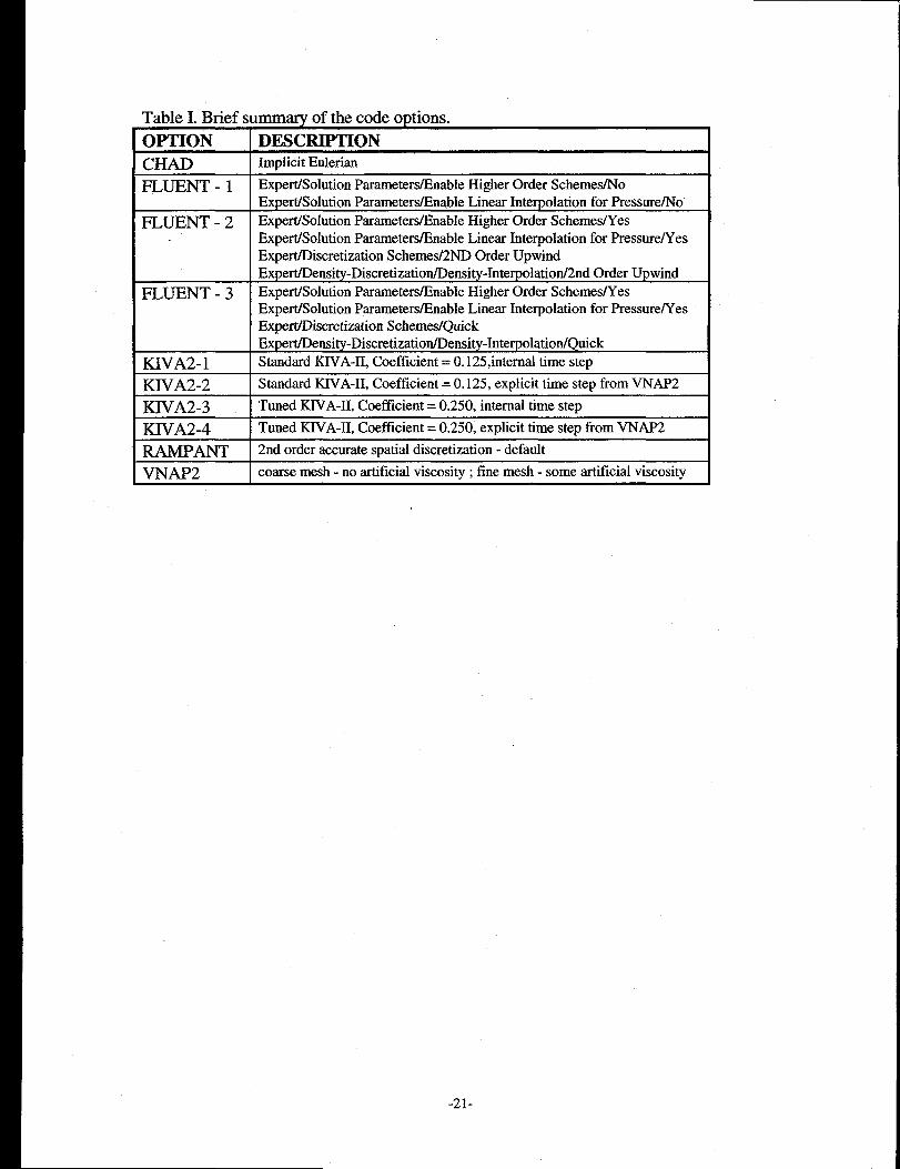
Table I. Briefs

OPTION

CHADFLUENT -1

FLUENT -2

FLUENT -3

KIVA2-1KIVA2-2

mlmaty of the code options.

DESCRIPTION IImplicit Eulerian IExpert/Solution Parameters/Enable H@er Order Schemes/NoExpert/Solution Parameters/Enable Linear Interpolation for Pressure/NoExpert/Solution Parameters/EnabIe Higher Order SchemesNesExpert/Solution Parameters/Enable Linear Interpolation for PressureNesExpertlDiscretization Schemes/2ND Order UpwindExpert/Density-Discretization/Density-Interpolation/2nd Order UpwindExpert/Solution Parameters/Enable Higher Order SchemesNesExpert/Solution Parameters/Enable Linear Interpolation for PressureNesExpert7Discretization Schemes/QuickExpe@ensity-Discretizatio~ensity-Inte~olatiotiQuickStandard KIVA-11,Coetlicient = O.125,interna1 time step

Standard KIVA-H, Coefficient= 0.125, explicit time step from VNAP2

KIVA2-3 Tuned KIVA-11,Coefficient= 0.250, internal time step

KIVA2-4 Tuned KIVA-11,Coefficient= 0.250,explicittime step fromVNAP2

RAMPANT 2nd order accurate spatial discretization - default

VNAP2 coarsemesh- no artificialviscosity; tine mesh- someartificialviscosity

-21-

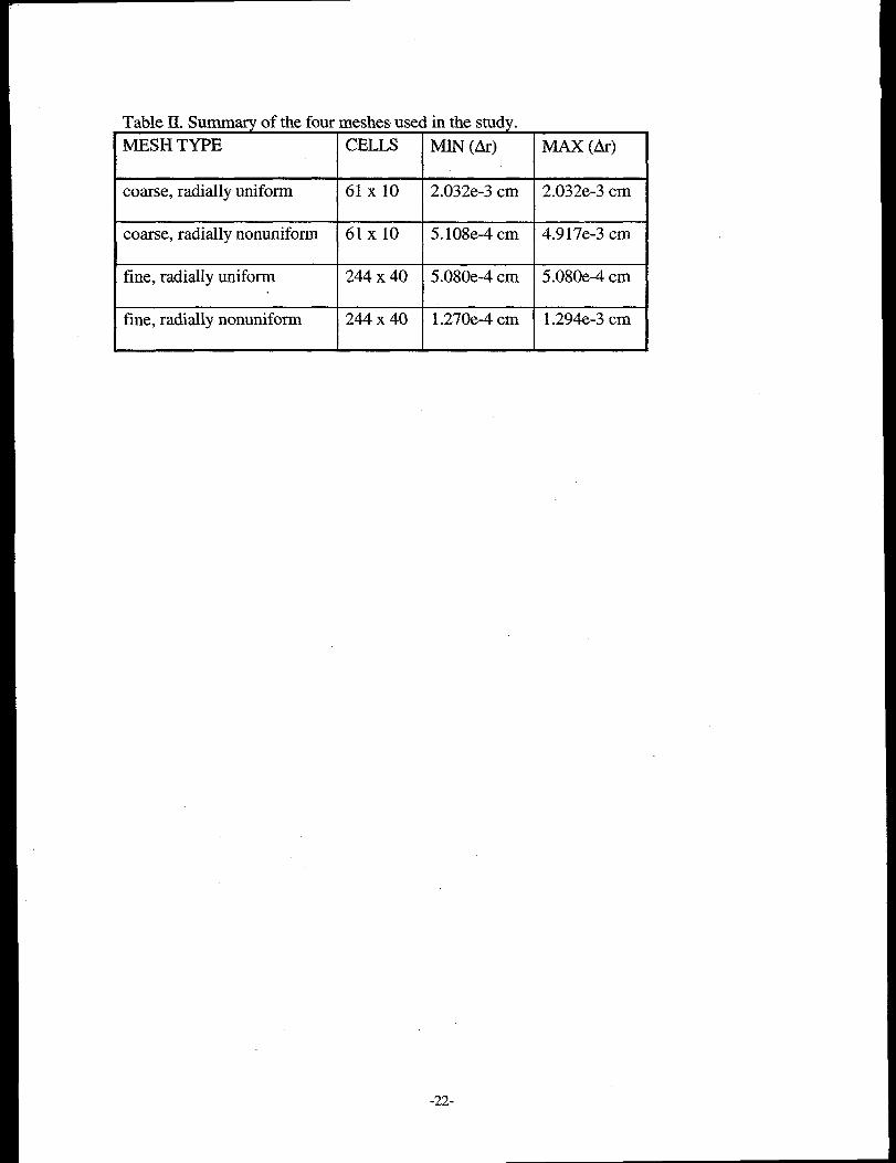
T-hla Tl Cmnm.mw nf tha fn,,r m(achnc. ,xca.-l ;n tha cti,rlwx Uulw u. UUIAIIIXLU y w. .lIU Lvul lIIVOXIUO Uovu .tLx Ulv C.LUUJ .

MESH TYPE CELLS MIN {AI’) MAX (Ar)

coarse, radially uniform 61 X 10 2.032e-3 cm 2.032e-3 cm

coarse, radially nonuniform 61 X 10 5. 108e-4 cm 4.917e-3 cm

fine, radially uniform 244 x 40 5.080e-4 cm 5.080e-4 cm

fine, radially nonuniform 244 x 40 1.270e-4 cm 1.294e-3 cm

-22-

0.0635

R (m)

0.0-0.0555 Z (m) 0.185

Figure 1. The coarse, radially uniform mesh is shown. At any point along the axialdirection, the radial spacing is uniform along the radial direction.

-23-

I

1.45

1.35

1.25

1.05

0.95

0.85

0.750.0

----------------- CHAD

—- —-— ----- RAMPANT I-------------------- FLUENT -2

--------------------------------KIVA2 -4

c EXPERIMENT

#*

0/

*/ 0+0“-/----- .--~.-.-.-,------

0.2 0.4r/R

0.6 0.8 1.0

Figure 2. Summary of the Mach number as a function of the dimensionless radius for allthe codes on a coarse, radially uniform mesh. The solid line is the most accurate codesolution.

-24-

-

-ClzoCLKw

18

16

14

12

10

8

6

4

2

0 L 11

Figure 3. Summary of the average error from the experimental data for all the codeoptions on a coarse, radially uniform mesh.

-25-

1.45

1.35

1.25

0.95

0.85

0.75

----------------- FLUENT- 1

FLUENT -2

--------------------------------FLUENT -3

● EXPERIMENT ,’”.*’

0.0 0.2 0.4 0.6 0.8 1.0r/R

Figure 4. Summary of the Mach number as a function of the dimensionless radius for thethree FLUENT options on a coarse, radially uniform mesh. The solid line is the mostaccurate FLUENT solution.

-26-

1.45

1.35

1.25

z

0.95

0.85

(

0.75

.------ ------- ---

---- ---- -

——— —-

KIVA2 -1

KIVA2 -2

KIVA2 -3

KIVA2 -4

● EXPERIMENT 4

------!

-.--

--

-----

------

0.0 0.2 0.4r/R

0.6 0.8 1.0

Figure 5. Summary of the Mach number as a function of the dimensionless radius for thefour KIVA2 options on a coarse, radially uniform mesh. The solid line is the mostaccurate K.IVA2 solution.

-27-

1.45

1.35

1.25

0.95

0.85

0.75

----------------- CHAD

—.—- —-—- —- RAMPANT

-------------------- FLUENT-3

----------------------------------KIVA2-4

VNAP2

0.0 0.2 0.4 0.6 0.8 1.0r/R

Figure 6. Summary of the Mach number as a function of the dimensionless radius for allthe codes on a coarse, radially nonuniform mesh. The solid line is the most accurate codesolution.

-28-

18

16

2

0

data for different code

t I I I I I

n Y CN m d- 1- al

Figure 7. Sumrnaryof the average error from the experimentaloptions on a coarse, radially nonuniform mesh.

-29-

1.45

1.35

1.25

z

0.95

0.85

0.75

<

----------------- FLUENT- 1

--------------------------------FLUENT -2

● EXPERIMENT

------- -

0.0 0.2 0.4 0.6 0.8 1.0r/R

Figure 8. Summary of the Mach number as a function of the dimensionless radius for thethree FLUENT options on a coarse, radially nonuniform mesh. The solid line is the mostaccurate FLUENT solution.

-30-

1.45

1.35

.25

.1’5

~ 1.05z

0.95

0.85

0.75

------------------- CHAD ~

--—- —--- —-— RAMPANT

---------------------- FLUENT -3

------------------------------------KIVA2 -41

VNAP2

/

1’#

● EXPERIMENT/’

1’

/’

1’

1’

0

0

*

#

.

—--

0.0 0.2 0.4 0.6 0.8 1.0r/R

Figure.9. Summary of the Mach number as a function of the dimensionless radius for allthe codes on a fine, radially uniform mesh. The solid line is the most accurate codesolution.

-31-

CKw

4

3

2

1

0 -L J- L L .1- J_

Figure 10. Summary of the average error from the experimental data foroptions on a fine, radially uniform mesh.

different code

-32-

CLLu

5!2

1.45

1.35

1.25

1.15

0.95

0.85

0.75

----------------- FLUENT-1

-------------------------------”FLUENT-2

FLUENT-3

● EXPERIMENTi

0.0 0.2 0.4 0.6 0.8 1.0r/R

Figure 11. Summary of the Mach number as a function of the dimensionless radius for thethree FLUENT options on a fine, radially uniform mesh. The solid line is the mostaccurate FLUENT solution.

-33-

1.45

Ifl:z

1.35

1.25

1.15

0.95

0.85

4

0.75

CHAD

—.—- --—- —-- RAMPANT

---------------------- FLUENT -3

-------------------------------------KIVA2 -4

---- ---- -- VNAP2

● EXPERIMENT

#

.------

0.0 0.2 0.4r/R

0.6 0.8 1.0

Figure 12. Summary of the Mach number as a function of the dimensionless radius for allthe codes on a fine, radially nonuniform mesh. The solid line is the most accurate codesolution.

-34-

4

%3w(YotYuIU2UJo2:1

0na5

Figure 13.options on

-L 1

an<z>

Summary of the average error from the experimental data for different codea fine, radially nonuniform mesh.

-35-

0.0356

R (m)

o0.0559

Z (m)0.0965

Figure 14. Comparison of experimental data points (symbols) and CHAD-calculatedMach number contours on a fine, radially uniform mesh.

-36-