Embed Size (px)
Citation preview

LA-13721-TThesis
The Chain-Length Distribution in
Subcritical Systems
LosN A T I O N A L L A B O R A T O R Y
AlamosLos Alamos National Laboratory is operated by the University of Californiafor the United States Department of Energy under contract W-7405-ENG-36.
Approved for public release;distribution is unlimited.

This thesis was accepted by the Department of Nuclear Engineering,Texas A & M University, College Station, Texas, in partial fulfillment ofthe requirements for the degree of Doctor of Philosophy. The text andillustrations are the independent work of the author and only the frontmatter has been edited by the CIC-1 Writing and Editing Staff to conformwith Department of Energy and Los Alamos National Laboratorypublication policies.
An Affirmative Action/Equal Opportunity Employer
This report was prepared as an account of work sponsored by an agency of the United StatesGovernment. Neither The Regents of the University of California, the United StatesGovernment nor any agency thereof, nor any of their employees, makes any warranty, expressor implied, or assumes any legal liability or responsibility for the accuracy, completeness, orusefulness of any information, apparatus, product, or process disclosed, or represents that itsuse would not infringe privately owned rights. Reference herein to any specific commercialproduct, process, or service by trade name, trademark, manufacturer, or otherwise, does notnecessarily constitute or imply its endorsement, recommendation, or favoring by The Regentsof the University of California, the United States Government, or any agency thereof. Theviews and opinions of authors expressed herein do not necessarily state or reflect those ofThe Regents of the University of California, the United States Government, or any agencythereof. Los Alamos National Laboratory strongly supports academic freedom and aresearcher's right to publish; as an institution, however, the Laboratory does not endorse theviewpoint of a publication or guarantee its technical correctness.

The Chain-Length Distribution inSubcritical Systems
Steven Douglas Nolen
LA-13721-TThesis
Issued: June 2000
LosN A T I O N A L L A B O R A T O R Y
AlamosLos Alamos, New Mexico 87545
v
ACKNOWLEDGMENTS
This research reflects the efforts and impact of many individuals. The author
would like to thank Dr. Theodore Parish for serving as the committee chair, and
moreover, for his understanding, support, and constant encouragement throughout this
research. The author would also like to express sincere appreciation to Dr. Gregory
Spriggs of the Los Alamos National Laboratory for serving as the principal advisor to
this dissertation. His infectious vision and vast experience with subcritical experiments
at the LANL Pajarito site have made this research a continually rewarding and
informative process. I would also like to thank the other members of my committee,
Drs. Marvin Adams, Yassin Hassan, Dante DeBlassie and Paulette Beatty for their
commitment of time and energy.
I would like to thank a number of people at Los Alamos National Laboratory
who contributed to this dissertation. First, I would like to thank each of the many group
leaders that have lent their support. I am profoundly grateful to Stephen Lee who first
envisioned MC++, who taught me C++, and who encouraged me to take the long, hard
road to a Ph.D. I am also grateful for the Monte Carlo knowledge obtained during
numerous conversations with Dr. Art Forster and Dr. Forrest Brown. I would like to
thank Julian Cummings and the Blanca code team for their advice and assistance in
working out the technical details of a production code.
Dr. Bob Busch at the University of New Mexico also has my appreciation for
providing access to their university’s AGN reactor.

vi
A special thanks goes to my colleagues and peers at the laboratory including
Chris Gesh, Kelly Thompson, Jon Dahl, and David Court. In addition to their
unswerving friendship and encouragement, I have benefited from their example proving
that this graduate degree can be achieved.
I am truly grateful for the love and support of my entire family. My parents,
Cecil and Lynette, have always stood by me, trusted me, and provided a home with
unconditional love. My sister and brother-in-law, Cindy and Alan, have always had an
open door for me even during the tough times. They were there many times with my
nephew and niece, Jarrett and Connor, to give me a break and a smile. My brother,
Greg, was probably my closest supporter and confidant. I can never thank him enough
for running the numerous errands when I was away from campus and for the solid
support I found in him. April’s parents, Dick and Judy, provided some much needed
financial support and some even more needed encouragement that comes from
experience. My wife, April, I mention last though she has been through the most. Her
ability to adapt and press on during these years still amazes me. In the midst of it all, she
still found time to impact peoples’ lives for Christ, and mine was not the least.
My final and most ardent thanks belongs to my Lord and Savior, Christ, who has
been my comfort and compass.
vii
TABLE OF CONTENTS
Page
ACKNOWLEDGMENTS..................................................................................................v
TABLE OF CONTENTS ................................................................................................ vii
LIST OF FIGURES .......................................................................................................... ix
LIST OF TABLES.......................................................................................................... xiii
ABSTRACT .....................................................................................................................xv
CHAPTER
I INTRODUCTION ............................................................................................1
II THEORY ..........................................................................................................7
A. Definition of a Fission Chain...................................................................7 B. Chain-Length Distribution.....................................................................14 C. Neutron Number Distribution................................................................16 D. Probability of Short Chains ...................................................................20 E. Galton-Watson Process..........................................................................24 F. Rossi and Feynman................................................................................26 G. Definition of Subcritical Multiplication ................................................29 H. Equivalent Fundamental-Mode Source .................................................31 I. Neutron Noise Analysis.........................................................................33 J. Correlated Pairs .....................................................................................37
III COMPUTATIONAL APPROACH ...............................................................41
A. Chain......................................................................................................41 B. MC++.....................................................................................................45 C. Analytic Cross Sections.........................................................................51 D. Noise Analysis in MC++ .......................................................................53 E. Handling the Background Noise............................................................54
IV NUMERICAL RESULTS ..............................................................................57
A. Code Validation.....................................................................................58 B. Effects of Prompt Multiplication Factor, K...........................................59 C. Effects of Multiplicity Distribution .......................................................67
viii
CHAPTER Page
D. Effects of Average Prompt Multiplicity, pν .........................................71 E. Effects of the Initial Source ...................................................................75 F. Effect on Noise Analysis .......................................................................80 G. Chain Time Dependence .......................................................................86 H. Time Analysis of the Prompt Fission Chains ........................................88 I. Spatial Harmonics..................................................................................93 J. Overall Detection Efficiency Considerations ........................................97
V CONCLUSIONS ..........................................................................................101
A. Summary..............................................................................................101 B. Future Work.........................................................................................102
REFERENCES ...............................................................................................................105
VITA...............................................................................................................................111

ix
LIST OF FIGURES
FIGURE Page 1 Example of prompt fission chains. .........................................................................4
2 Neutron activity vs. time in a multiplying system................................................11
3 Neutron activity vs. time in a non-multiplying system. .......................................12
4 Chain-length distribution for a K=0.99. ...............................................................16
5 Comparison of Frehaut distribution with binary (analog MCNP) distribution. ...20
6 Branching potential for a typical neutron in a multiplying system. .....................21
7 Chain-length distributions for Frehaut and binary distributions at 2.42pν = ......25
8 Propagation of two prompt fission chains. ...........................................................35
9 Determining neutron interaction correlations.......................................................36
10 Resolving the background noise threshold. ..........................................................56
11 Chain-length distributions for select values of K. ................................................61
12 Integral of the chain-length distribution showing its relationship to the subcritical prompt multiplication, Mp. ..................................................................65
13 Differential subcritical prompt multiplication contribution of chain lengths L>1 for various K..................................................................................................66
14 Effect of neutron multiplicity on the chain-length distribution in a highly subcritical system. (K=0.5 and pν =2.268.) ..........................................................68
15 Effect of neutron multiplicity on the chain-length distribution in a highly subcritical system. (K=0.5 and pν =3.2076) .........................................................69
16 Effect of neutron multiplicity on the chain-length distribution in a slightly subcritical system. (K=0.99 and ν =2.268.) .........................................................70
17 Effect of neutron multiplicity on the chain-length distribution in a slightly subcritical system. (K=0.99 and pν =3.2076) .......................................................71

x
FIGURE Page 18 pν effects on the chain-length distribution at K=0.5.............................................73
19 pν effects on the chain-length distribution at K=0.99...........................................74
20 pν effects on the integral subcritical prompt multiplication. ...............................75
21 Spatial effects on the chain-length distribution caused by the source configuration. (K=0.7) ..........................................................................................77
22 Spatial effects on the chain-length distribution caused by the source configuration (K=0.99) .........................................................................................78
23 Source configuration effect on system subcritical prompt multiplication calculation (K=0.7). ..............................................................................................79
24 Source configuration effect on the system multiplication calculation (K=0.99)................................................................................................................80
25 Theoretical maximum number of correlated pairs of neutrons per source neutron from an EFM source................................................................................82
26 Expected number of correlated pairs from a capture detector with an efficiency of 100% for various K. .......................................................................84
27 Expected number correlated pairs using a capture detector with an efficiency of 10% for various K. ...........................................................................................85
28 Average duration of a fission chain vs. prompt neutron lifetime. ........................87
29 Ratio of fission chain duration to the prompt neutron lifetime vs. K ...................88
30 Bare, enriched uranium slab reactor. ....................................................................89
31 Results for a simulated Rossi-α measurement performed on a bare enriched uranium slab. ........................................................................................................90
32 Enriched uranium reactor with water reflector.....................................................91
33 Dual decay mode Rossi-α curve in reflected slab reactor. ...................................92
34 Expanded view of Rossi-α curvature. ..................................................................93
35 Spatial harmonics appearing in bare slab geometry. ............................................94

xi
FIGURE Page 36 Bare slab with enriched uranium showing harmonics..........................................96
37 Effect of population type sampled on Rossi-α data. ............................................99
38 Signal degradation due to decreasing detector efficiency. .................................100

xii

xiii
LIST OF TABLES
TABLE Page I Statistical analysis of neutron population shown in Figures 2 and 3....................13
II Frehaut’s fitting parameters..................................................................................17
III Frehaut's original and corrected distributions......................................................19
IV Analytic cross section set corresponding to Pu. ..................................................53
V Comparison of analytic solution and point model Monte Carlo Solution for K=0.3 with pν =2.268 for chain lengths 1 through 7. ...........................................59
VI Comparison of analytic solution and point model Monte Carlo solution for K=0.99 with pν =3.2076 for chain lengths 1 through 7. .......................................59
VII Multiplication obtained during various Chain simulations. ................................63
VIII Parameters for dual Rossi-α curve fit..................................................................93
IX Parameters for regression fit of harmonic data....................................................95
X Parameters for dual exponential regression fit of bare enriched slab. .................97
XI Detector efficiency effect on fastest decay mode estimate..................................98

xiv

xv
ABSTRACT
The Chain-Length Distribution in Subcritical Systems. (May 2000)
Steven Douglas Nolen, B.S., Texas A&M University;
M.S., Texas A&M University
Chair of Advisory Committee: Dr. Theodore Parish
The individual fission chains that appear in any neutron multiplying system
provide a means, via neutron noise analysis, to unlock a wealth of information regarding
the nature of the system. This work begins by determining the probability density
distributions for fission chain lengths in zero-dimensional systems over a range of
prompt neutron multiplication constant (K) values. This section is followed by showing
how the integral representation of the chain-length distribution can be used to obtain an
estimate of the system’s subcritical prompt multiplication (MP). The lifetime of the
chains is then used to provide a basis for determining whether a neutron noise analysis
will be successful in assessing the neutron multiplication constant, k, of the system in the
presence of a strong intrinsic source. A Monte Carlo transport code, MC++, is used to
model the evolution of the individual fission chains and to determine how they are
influenced by spatial effects. The dissertation concludes by demonstrating how
experimental validation of certain global system parameters by neutron noise analysis
may be precluded in situations in which the system K is relatively low and in which
realistic detector efficiencies are simulated.

xvi

1
CHAPTER I
INTRODUCTION
Criticality safety is vitally important in the nuclear industry. If there were any
doubts about this, these should have disappeared after the accident in Tokai-mura, Japan
last year.1 On September 30, 1999, three workers were seriously injured when they
inadvertently created a super-critical configuration of uranyl nitrate solution at a fuel-
reprocessing plant. As with any industrial process, there are always some associated
risks in the nuclear industry, but these risks can be minimized with continued research
and development in the area of operational safety. This assertion is particularly valid in
the field of criticality safety where there has been an obvious need to develop accurate
and reliable techniques to provide continuous monitoring of the subcriticality of nuclear
processing and storage facilities. These types of monitoring systems differ from the
current criticality alarm systems found in most plants that trip at setpoints that indicate
that criticality has already occurred. Had a continuous monitoring system been in place
in Tokai-mura rather than a criticality alarm system, this accident might have been
averted.
Presently, there are several techniques for measuring the effective neutron
multiplication constant, k, in reactor systems operating near delayed critical. However,
as systems become more and more subcritical, only a few of these techniques are general
enough that they can be adapted to perform in-situ subcriticality measurements in
This dissertation follows the style and format of Nuclear Science and Engineering.

2
process and storage facilities. Of these techniques, neutron noise analysis is certainly an
attractive option. For highly subcritical systems, however, the neutron noise signal
becomes complex, and its interpretation becomes somewhat more difficult.
Accordingly, a better understanding of neutron noise techniques and their relation to
important system parameters, such as k, is needed to increase our ability to accurately
unfold signals from subcritical systems. Armed with additional understanding, it may be
possible to develop new monitoring systems that will provide nuclear workers with early
warning systems if criticality safety limits are being approached.
Traditionally, two distinct research areas have carried the label neutron noise
analysis. The first of these deals with observing fluctuations in a reactor’s power level
and correlating these changes with naturally occurring or mechanically induced physical
disturbances occurring elsewhere in the reactor system. Examples of such disturbances
include the growth and collapse of bubbles in the core of a boiling water reactor, the
opening and closing of a relief valve, or the rotation of a special rod oscillator at some
prescribed frequency. Unlike that due to the stochastic nature of individual prompt
fission chains, this type of neutron noise is inherently deterministic with respect to the
response of the neutron population. While it will not receive further attention here, there
are a number of books on power reactor noise theory by Thie and others.2,3
The second type of research termed neutron noise analysis deals with the
observation of individual prompt fission chains and the correlation of the resulting
microscopic fluctuations of the neutron population with physical parameters of the
system. This type of neutron noise analysis was first performed by researchers at the

3
Los Alamos National Laboratory (LANL) while experimenting with zero-power,
critical-mass assemblies.4-8 They noted that the neutron leakage flux exhibited larger-
than-expected random fluctuations. Bruno Rossi proposed that these fluctuations
corresponded to sharp changes in the neutron population as individual prompt fission
chains spawned and then died-out on a time scale characterized by the neutron lifetime
of the system.8 In systems in which the mean time between source neutron births is
significantly greater than the average life span of a prompt fission chain, the neutrons in
the system appear in brief bursts, or clumps. As these clumps of neutrons die-out, the
neutron population temporarily dips to zero until another prompt fission chain begins to
spawn. The analysis of the observed statistical fluctuations in the neutron population has
been explored by a number of researchers.9-15 An example of the clumping phenomena
is illustrated in Figure 1 which shows the neutron reaction rate as the number of
observed events that occur within 0.125 µsec. wide intervals.

4
Time [sec]
0.00000 0.00002 0.00004 0.00006 0.00008 0.00010
Neu
tron
Rea
ctio
n R
ate
0
100
200
300
400
500
Fission Chains Source Neutrons
Figure 1. Example of prompt fission chains.
In this example, note that the neutron population is zero for a significant portion
of the time. The exact length of time over which the population is zero depends highly
on the strength of the driving source, the prompt neutron multiplication factor, K, and the
prompt neutron lifetime, τ. The prompt neutron multiplication factor is defined as
( )1eff effK k β= − , where keff is the effective neutron multiplication factor and βeff is the effective delayed
neutron fraction. The zero-population intervals are quite evident in the bare, metal
Godiva assembly because of its very short neutron lifetime. If the assembly is driven
5
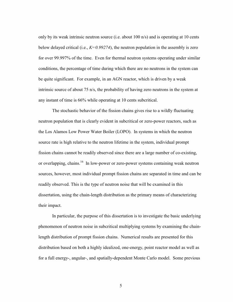
only by its weak intrinsic neutron source (i.e. about 100 n/s) and is operating at 10 cents
below delayed critical (i.e., K=0.99274), the neutron population in the assembly is zero
for over 99.997% of the time. Even for thermal neutron systems operating under similar
conditions, the percentage of time during which there are no neutrons in the system can
be quite significant. For example, in an AGN reactor, which is driven by a weak
intrinsic source of about 75 n/s, the probability of having zero neutrons in the system at
any instant of time is 66% while operating at 10 cents subcritical.
The stochastic behavior of the fission chains gives rise to a wildly fluctuating
neutron population that is clearly evident in subcritical or zero-power reactors, such as
the Los Alamos Low Power Water Boiler (LOPO). In systems in which the neutron
source rate is high relative to the neutron lifetime in the system, individual prompt
fission chains cannot be readily observed since there are a large number of co-existing,
or overlapping, chains.16 In low-power or zero-power systems containing weak neutron
sources, however, most individual prompt fission chains are separated in time and can be
readily observed. This is the type of neutron noise that will be examined in this
dissertation, using the chain-length distribution as the primary means of characterizing
their impact.
In particular, the purpose of this dissertation is to investigate the basic underlying
phenomenon of neutron noise in subcritical multiplying systems by examining the chain-
length distribution of prompt fission chains. Numerical results are presented for this
distribution based on both a highly idealized, one-energy, point reactor model as well as
for a full energy-, angular-, and spatially-dependent Monte Carlo model. Some previous

6
work in this area has been preformed by Mihalczo et al. using KENO-NR in which they
calculated the chain-length distribution for a BWR operating at a k=0.9.17,18 The aim of
this dissertation is to extend this work by increasing the resolution of the chain-length
distribution and by examining a K range from 0.3 to 0.999. Results will also be present
for the chain-length distributions produced by a variety of neutron source distributions
and including various spatial effects that occur in single and multi-region systems.
Moreover, the role of the overall detector efficiency in neutron noise measurements will
be examined to demonstrate how low detector efficiencies can preclude the accurate
estimation of system parameters when using neutron noise-based techniques in highly
subcritical systems.

7
CHAPTER II
THEORY
In this chapter, the fundamental concepts of neutron noise theory are presented
beginning with the definition of a fission chain and a demonstration of how it
characterizes the behavior of a neutron multiplying system. Next, the chain-length
distribution is introduced and a description is provided on how the neutron multiplicity
and the source distribution determine its form. The introduction of the chain-length
distribution concept is followed by a mathematical representation of the noise problem
based on a point kinetics model. Finally, the chapter concludes by showing how neutron
noise can be used to reveal some global parameters that characterize the subcritical
neutron multiplying system.
A. Definition of a Fission Chain
The term fission chain refers to any neutrons that appear in a system that are
related to a common ancestor or initiating source neutron. In determining the total
number of neutrons in a chain, only the source neutron and the prompt fission neutrons
are considered. In a multiplying system, the source neutrons originate in a variety of
ways including: 1) external sources (i.e., special reactor components such as Pu-Be
startup sources), 2) intrinsic sources, where the neutrons are emitted from spontaneous
fission events occurring randomly throughout the nuclear fuel, and 3) delayed neutron
sources that arise from the radioactive decay of certain fission products. Although
delayed neutron precursors are generated from fission events that occur as a part of a
8
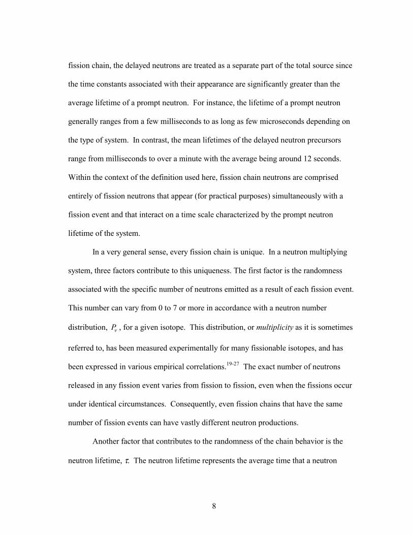
fission chain, the delayed neutrons are treated as a separate part of the total source since
the time constants associated with their appearance are significantly greater than the
average lifetime of a prompt neutron. For instance, the lifetime of a prompt neutron
generally ranges from a few milliseconds to as long as few microseconds depending on
the type of system. In contrast, the mean lifetimes of the delayed neutron precursors
range from milliseconds to over a minute with the average being around 12 seconds.
Within the context of the definition used here, fission chain neutrons are comprised
entirely of fission neutrons that appear (for practical purposes) simultaneously with a
fission event and that interact on a time scale characterized by the prompt neutron
lifetime of the system.
In a very general sense, every fission chain is unique. In a neutron multiplying
system, three factors contribute to this uniqueness. The first factor is the randomness
associated with the specific number of neutrons emitted as a result of each fission event.
This number can vary from 0 to 7 or more in accordance with a neutron number
distribution, Pν , for a given isotope. This distribution, or multiplicity as it is sometimes
referred to, has been measured experimentally for many fissionable isotopes, and has
been expressed in various empirical correlations.19-27 The exact number of neutrons
released in any fission event varies from fission to fission, even when the fissions occur
under identical circumstances. Consequently, even fission chains that have the same
number of fission events can have vastly different neutron productions.
Another factor that contributes to the randomness of the chain behavior is the
neutron lifetime, τ. The neutron lifetime represents the average time that a neutron

9
exists before it undergoes some event that removes it from the system (i.e., an absorption
or leakage). Similarly to the randomness in the number of neutrons emitted per fission,
the actual time between removal events varies even for neutrons with identical starting
conditions. The exact time of removal is distributed exponentially in time,
( )t dtp t dt e τ
τ−
= ,
where τ is the neutron removal lifetime, and ( )p t dt is the probability that a neutron will
survive until time, t, and then be removed from the system in the time interval dt about t.
The final factor that contributes to the randomness of the chain behavior is the
probability that an event of a particular type will occur. In any neutron multiplying
system, a neutron can interact with surrounding medium by means of a large number of
nuclear reactions. These include fission, parasitic absorption, elastic and inelastic
scattering, leakage, and so forth. For this research, the probability for causing a fission
event, fP , is the most important.
Because of these three random factors, it is impossible to predict the exact
behavior of any given fission chain. Nevertheless, when a large number of chains are
sampled, the aggregate behavior of the fission chains becomes quite predictable. This
situation is analogous to the rolling of a single die. It is impossible to predict which
number will appear on any given roll, but, on an average, it is possible to show that each
number has an equal probability of 1/6th for appearing. Similarly, neutron noise theory
is based on predicting the average behavior of a large number of individual, random
chains.

10
To further understand the concept of a fission chain and its inherent randomness,
a detector’s response to a neutron multiplying system has been simulated for a small
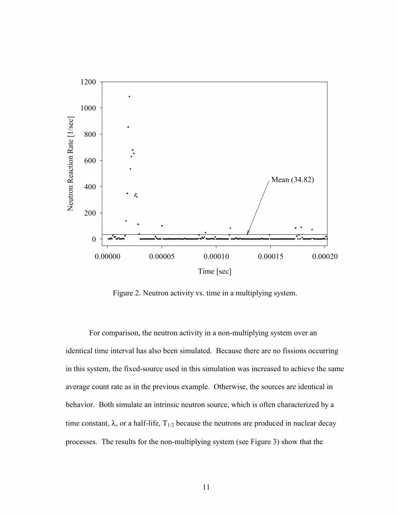
interval of time. These results are shown in Figure 2. The prompt neutron
multiplication factor, K, for this system was 0.99, which in accordance with the source
multiplication equation,
11pM
K=
− , (II.1)
yields a prompt subcritical multiplication, Mp, of 100. For this simulation, 100 source
neutrons were randomly put into the system at a rate of 55 10 secn⋅ . The source
neutrons then spawned several fission chains producing a total of 6,934 fission neutrons
over a simulated run time of about 0.2 msec. When divided into equal channel widths of
1 µsec, the average number of reactions appearing per channel was calculated to be
34.82. However, because of the tight groupings of the neutrons within the fission
chains, most of the channels recorded zero events. In fact, the majority of the observed
events (roughly 80% of the total counts over the counting interval) came from a single
fission chain, which only lasted about ~13 µsec. This illustrates what the Los Alamos
researchers observed as fluctuations in the neutron intensity.4
11
Time [sec]
0.00000 0.00005 0.00010 0.00015 0.00020
Neu
tron
Rea
ctio
n R
ate
[1/s
ec]
0
200
400
600
800
1000
1200
Mean (34.82)
Figure 2. Neutron activity vs. time in a multiplying system.
For comparison, the neutron activity in a non-multiplying system over an
identical time interval has also been simulated. Because there are no fissions occurring
in this system, the fixed-source used in this simulation was increased to achieve the same
average count rate as in the previous example. Otherwise, the sources are identical in
behavior. Both simulate an intrinsic neutron source, which is often characterized by a
time constant, λ, or a half-life, T1/2 because the neutrons are produced in nuclear decay
processes. The results for the non-multiplying system (see Figure 3) show that the

12
counts per 1 µsec channel are randomly distributed about the mean value of 34.82 as
expected from a Poisson type distribution. Because there are no fission chains, there is
no clustering of neutrons.
Time [sec]
0.00000 0.00005 0.00010 0.00015 0.00020
Neu
tron
per C
hann
el [1
/sec
]
0
10
20
30
40
50
60
70
80
90
100
Mean (34.82)
Figure 3. Neutron activity vs. time in a non-multiplying system.
As expected from the results shown in Figures 2 and 3, the variance of the counts
per channel is significantly different for the two cases (see Table I). The increase in the
variance for the multiplying system is a result of the clustering of the neutrons during the
prompt fission chains. For the non-multiplying system shown in Figure 3, the counts per
channel reflect the randomness of the source and are distributed about the mean value in

13
a Poisson fashion. That is, 99.7% of the channel counts should fall within 3 standard
deviations about the mean. As can be noted from Table I, 100% of all the counts in this
simulation fell within this tolerance. For the multiplying system shown in Figure 2, this
is clearly not the case. Over half of the channels contain zero counts, and a select few
have a very large number of pulses due the fission chains.
TABLE I
Statistical analysis of neutron population shown in Figures 2 and 3.
K Total Neutrons
Total Duration
µµµµsec
Average Channel Counts
Variance2σ Max Min
0.00 7034 201.57 34.8218 38.9 53 190.99 7034 201.35 34.8218 18,765.2 1087 0
The variance of the channel counts clearly indicates a phenomenon that cannot
be adequately described using deterministic methods. The stochastic nature of the
prompt fission chains has been previously studied by numerous authors who have noted
that the average behavior of the neutron population can be a secondary factor as
compared to the behavior of the individual neutrons in these systems.6,28-39 For this
reason, each fission chain is propagated independently in energy, angle, and space rather
than estimating the chain’s behavior based on an approximation of the average chain.

14
B. Chain-Length Distribution
The evolution of a fission chain can be summarized as follows. Counting the
single source neutron (i.e., external, intrinsic, or delayed neutron) that acts as an initiator,
the exact number of neutrons spawned within a particular fission chain will be purely a
matter of chance. Each neutron in the chain will either induce a fission event in the
system, resulting in additional neutrons in the chain’s population, or it will disappear
from the system due to leakage or parasitic absorption. (Note scattering events do not
remove neutrons from the chain because the chain population does not depend on
neutron energy or direction in the system.) As might be expected, the conglomeration of
random events results in the appearance of chains with varying total neutron populations
(i.e. lengths). Furthermore, chains with identical lengths may also differ with respect to
the number and types of events occurring within them. Rather than identifying each
chain according to the exact series of events that occurs during the chain’s evolution, the
chains will be classified according to their total neutron population hereafter referred to
as their final length, L. Further, ( )P L is defined as the probability per source neutron
for observing a fission chain of length L. It is also worth emphasizing that L can only

15
take on discrete values, i.e., integers. The chain-length distribution discussed herein, is
just a set of lengths, L, and their associated probabilities, ( )P L , that uniquely
characterize the multiplying system.
Provided the multiplying system can be characterized by known or measurable
global parameters, such as K and pν , the corresponding chain-length distribution is
highly predictable and can be readily determined using Monte Carlo techniques. An
example of a chain-length distribution is shown below in Figure 4. The figure shows the
probability that a source neutron will spawn a fission chain of a specified length. As
expected from Figure 2, the shortest chain length, comprised of only the source neutron,
is the most frequently occurring. With the exception of the shorter chains, the
probability decreases almost monotonically with increasing length. Although longer
chain lengths may occur, the longest length shown represents a chain containing several
hundred thousand neutrons, and it would be expected to occur only once per 1014 source
neutrons ( )( )5 145 10 10P L −= ⋅ � . A more in-depth treatment explaining the shape of
the distribution including its tails appears in the following sections.

16
Chain Length
100 101 102 103 104 105 106
Prob
abili
ty o
f Obs
ervi
ng a
Cha
in o
f Len
gth
L
10-1510-1410-1310-1210-1110-1010-910-810-710-610-510-410-310-210-1100
Figure 4. Chain-length distribution for a K=0.99.
C. Neutron Number Distribution
To better understand the nature of the chain’s behavior, it is useful to begin with
an examination of the multiplicity distribution of the fission neutrons, ( )P ν . In almost
every book on neutron or reactor physics, the only value mentioned in regard to this
distribution is its mean value designated as ν or for prompt neutrons pν . Because ν is
the property that commonly appears in deterministic equations used to describe the
fission neutron source in a multiplying system, it is also the parameter included in

17
typical neutron cross section files as the product of fν Σ . The full distribution for the
prompt component was first studied by researchers at the Los Alamos Scientific
Laboratory, such as Richard Feynman, who were intensely curious about the actual
shape of the distribution.6 Diven and Leachman measured the first ( )P ν distributions
for several isotopes basing their work on the kinetic energy of the fission fragments.20,21
They determined that the distributions appeared to have a binomial form. As the
distributions were revised over the years by various investigators for an ever-increasing
range of isotopes, the predicted shape began to change as well.22-27 In 1988, Frehaut
proposed a single distribution that sufficiently captured the multiplicity distributions for
a number of major isotopes.27 The distribution, which is expressed as a function of pν ,
provides a much better approximation than earlier relationships. In Frehaut’s ( )P ν
function, the fitting constants, a and b, are parameters associated with a particular ν .
The values associated with these parameters appear in Table II.
( )2
12
2
p
baP eb
ν ν
νπ
−� �− � �
� �= (II.2)
TABLE II
Frehaut’s fitting parameters
ν 0 1 2 3 4 5 6 >7
b 0.94 1.13 1.22 1.295 1.16 1.222 1.226 1.235a 2.827 1.073 1.075 1.095 0.953 0.958 1.048 1.000

18
While this distribution provides a means to model the multiplicity for a variety of
isotopes, there are some caveats. Frehaut mentioned that the fit was unsatisfactory for
thorium isotopes. Furthermore, the distribution is not normalized to 1.0, which means
that the pν used to construct the distribution is not the average value that would be
obtained from the final distribution. This lack of consistency can be understood because
Frehaut was more interested in matching his curves to the experimental data rather than
insuring that they were sufficient for a Monte Carlo type simulation. As an example of
these inconsistencies, the neutron number distribution for 2.42pν = has been calculated
(see Table III). The values appearing in the last column of Table III arise from a
modification to Frehaut’s original distribution necessitated by the need to normalize the
distribution and preserve pν . The adjustment was performed so as to have the least
impact on the most likely portion of the Frehaut distribution’s shape.
Besides using the Frehaut distribution, another more common approach for
specifying the multiplicity is to assume that the number of prompt neutrons emerging
from a fission is limited to the integers bounding pν . For example, if 2.5pν = , then it is
assumed that 50% of the fissions yield two neutrons, and the other 50% yield three
neutrons. This binary-distribution approach has proven to be suitable for calculations in
which the macroscopic behavior of the system is of primary interest. For example,
MCNP uses this technique when it is run in analog mode.40 To reduce the variance
when performing k-eigenvalue calculations, however, Monte Carlo packages generally
run in a nonanalog mode and use the value of pν or ν directly. Figure 5 shows the

19
Frehaut distribution as compared to the multiplicity distribution associated with binary
sampling.
TABLE III
Frehaut's original and corrected distributions.
Frehaut
νννν Binary Original Normalized Corrected 0 0.0 0.0436 0.0428 0.0425 1 0.0 0.1720 0.1685 0.1685 2 0.58 0.3313 0.3246 0.3246 3 0.42 0.3051 0.2990 0.2990 4 0.0 0.1296 0.1270 0.1270 5 0.0 0.0337 0.0330 0.0330 6 0.0 0.0048 0.0047 0.0047 7 0.0 0.0003 0.0003 0.0006
Total 1.00 1.0205 1.0000 1.0000
2.42 2.4680 2.4184 2.4200 Correction 0.0016

20
ν
0 1 2 3 4 5 6 7
P(ν)
0.0
0.1
0.2
0.3
0.4
0.5
0.6
Analog MCNPFrehaut
Figure 5. Comparison of Frehaut distribution with binary (analog MCNP) distribution.
D. Probability of Short Chains
The choice of the distribution can have a significant impact on the modeling of a
system when the microscopic behavior is important, as when analyzing the neutron
noise. The multiplicity distribution directly influences the way the neutrons start a
branching process during fission events. Ignoring the time dependence for a moment, a
probability tree can be constructed for each source neutron. The terminations, or leaves
of the probability tree, are comprised of the probability of not causing a fission and the
probability of causing a fission that does not release any neutrons. In the same way that

21
fissions that release zero neutrons terminate a branch; all other fissions create a number
of branches equal to the number of neutrons released. Figure 6 shows the beginnings of a
probability tree that represents the branching potential of a typical neutron in a
multiplying system.
P0
P1
P2
P3
P4
P5
P6
P7
Pf
1-Pf
Pf
1-Pf
Pf
1-Pf
Pf
1-Pf
1st
2nd
P0
P1
P2
P3
P4
P5
P6
P7
P0
P1
P2
P3
P4
P5
P6
P7
P0
P1
P2
P3
P4
P5
P6
P7
Figure 6. Branching potential for a typical neutron in a multiplying system.

22
In Figure 6, fP is the probability that a neutron will cause a fission, and nP is the
probability that a fission event will produce n neutrons. Using the probability-tree
approach, it is possible to compile the complete set of paths that result in a fission chain
of any specified length. While this is straightforward for short chains ( )7L ≤ , the
remaining chain-lengths become increasingly complex to account for as the potential
paths increase with increasing length. Tracing the paths for some of the shorter chains
has yielded the following observations.
There are actually three ways that a chain can have a length of 1. The most
obvious ways in which this may happen occur when the source neutron leaks out of the
system or is parasitically absorbed. Noting that either of these must happen if the source
neutron does not induce a fission, the total probability of their occurrence is simply
( )1 fP− . A slightly less obvious way to have a chain length of 1 occurs when the source
neutron causes a fission from which no neutrons are emitted. In this case, the fission
probability must be multiplied by the probability that the fission event produces zero
neutrons (i.e., 0fP P ). Hence, the probability of obtaining a chain of length equal to 1,
( )1P , from all three ways is
( ) ( ) 01 1 f fP P P P= − + . (II.3) Due to its recurrence in formulating the probabilities for chains with lengths greater than
1, the probability for a non-fission event, ( )1 fP− , and the probability for a fission event

23
producing zero neutrons, ( )0fP P , are combined into a single probability hereafter
denoted as the loss probability, lP . In addition to being the probability of observing a
chain with length equal to 1, lP is also the probability that any branch terminates.
( ) 01l f fP P P P= − + (II.4) To further simplify the following notation, it is useful to define the product of the fission
probability and the probability for releasing n neutrons as
fn f nP P P= . (II.5) Using this notational convention, the following relations can be used to calculate the
probability of a source neutron initiating chains with lengths of 2 through 7.
( ) 12 f lP P P= (II.6)
( ) 2 22 13 f l f lP P P P P= + (II.7)
( ) 3 2 33 1 2 14 3f l f f l f lP P P P P P P P= + + (II.8)
( ) ( )4 2 3 2 2 44 1 3 2 1 2 15 4 2 6f l f f f l f f l f lP P P P P P P P P P P P= + + + + (II.9)
( ) ( ) ( )5 4 2 2 3
5 2 3 1 4 1 3 1 2
3 2 51 2 1
6 5 10
10f l f f f f l f f f f l
f f l f l
P P P P P P P P P P P P P
P P P P P
= + + + +
+ + (II.10)
( ) ( )( ) ( )
6 2 56 2 4 1 5 3
2 3 4 3 2 31 2 3 1 4 2 1 3 1 2
4 2 61 2 1
7 6 6 3
30 15 5 20 30
15
f l f f f f f l
f f f f f f l f f f f l
f f l f l
P P P P P P P P P
P P P P P P P P P P P P
P P P P P
= + + +
+ + + + +
+ +
(II.11)
( ) 778 f lP P P= +� .
For even longer chain lengths, similar expressions can be written following the pattern
established above although the process becomes increasingly complex. Regardless of
the magnitude of K, the numerical solution of ( )P L obtained using Monte Carlo
techniques can be benchmarked against the analytic solutions given above for chain
24
lengths 1 through 7. As K nears 1.0, the numerical solution can also be benchmarked
against the asymptotic solution previously obtained for the Galton-Watson problem
described in Harris.41
E. Galton-Watson Process
When nuclear researchers first began to study the propagation of fission chains in
subcritical systems, they recognized that this problem was akin to an older problem that
had been studied since the 1800’s.41,42 Around this time, Francis Galton, a
mathematician, and the Reverend H. W. Watson, an amateur mathematician and
sociologist, were studying the fate of prominent families in Europe. In particular, they
were seeking to determine the probability of a particular surname disappearing from a
population given that each generation has an equal probability for having a specified
number of male progeny. Using census data, Galton and Watson constructed a
probability distribution of having 0, 1, 2, etc. sons for each of several generations and
found that the distributions were roughly constant across the generations. This type of
process later became known as a Markov process and is the predecessor of the
mathematics field of branching processes.
As in the Galton-Watson branching study, the choice of multiplicity distributions
can have a profound effect on the probability of observing fission chains of certain
lengths. Using the binary distribution given in Table III for 2.42pν = , it follows that a
chain length of 2 can never occur. If the original source neutron is parasitically absorbed
or leaks from the system, then the chain length will be 1. If, on the other hand, the

25
source neutron induces a fission, then either 2 or 3 neutrons will be produced, which
means the next possible chain contains at least 3 neutrons. Similarly, if pν =3.5, the
lengths of 2, 3 and 6 are prevented. The exclusion of these common fission chains can
be seen by observing how a system’s chain-length distribution is affected by the two
different multiplicity distributions.
Chain Length
100 101 102 103 104 105 106
Prob
abili
ty o
f a c
hain
of l
engt
h, L
10-1510-1410-1310-1210-1110-1010-910-810-710-610-510-410-310-210-1100101
Binary DistributionFrehaut Distribution
Figure 7. Chain-length distributions for Frehaut and binary distributions at 2.42pν = .
Using the binary distribution leads to significant differences as compared to the
Frehaut distribution at short chain lengths. As the chain lengths increase, the differences

26
become less noticeable. However, since the area under each chain-length distribution is
the same, the probability of observing longer chains is also affected (see Figure 7).
F. Rossi and Feynman
Bruno Rossi has been credited with recognizing that the larger-than-expected
oscillations in the neutron count rates observed in the Low-Power Water-Boiler Reactor
(LOPO) at Los Alamos were caused by the spawning and dying out of individual, fission
chains.4,8 Evidence for the fission chain theory was further provided by experiments
conducted by Wimmett et al. on the research reactor Godiva-II.43 They performed a
series of measurements in which they brought the bare, uranium-fueled reactor to $0.05
above prompt critical numerous times. The objective was to observe the time that it took
to reach a reference power level following the reactivity insertion. Immediately
following the reactivity insertion, the system was, of course, super-prompt critical.
However, for a measurable time after the reactivity insertion, the power level remained
roughly constant at the level of the intrinsic source because the vast majority of the
fission chains in the system would spawn and subsequently die out. The reactor power
would not increase dramatically until a persistent fission chain emerged. The times that
elapsed from insertion to power excursion were tabulated, and it was observed that the
scatter in the elapsed times could be explained only by a phenomenon like Rossi’s
fission chains. This experiment also showed that the system behaved in a stochastic
manner prior to the power excursion. Only after a chain reached a sufficiently large size

27
could a deterministic reactor model adequately represent the time-dependent behavior of
the system.
Of course, Rossi provided his own proof, too. He theorized that the random
behavior of the fission chains was actually governed by the properties of the multiplying
system.5 Conversely, the key to measuring these properties would depend on the ability
to detect and quantify the clumping phenomena (shown earlier in Figure 2). From the
power peaks observed in the LOPO, Rossi postulated that the neutrons from a single
chain evolved on a faster time scale, and as such, were more highly correlated in time
than the intrinsic source neutrons. Rossi’s proposal concerning the importance of the
fission chains and their time correlation intrigued his associate Feynman, who developed
much of the early background theory and equations describing neutron noise analysis.6
In addition to deriving the Rossi-α formula, Feynman also proposed his variance-to-
mean technique. In this technique, the ratio of the signal’s variance to its mean is
computed. If this ratio is significantly greater than 1.0, it implies that the signal arose
from phenomena other than a completely random distribution and that fission chains
must be present.
In developing the point-kinetic model for neutron noise, Feynman started with a
simple conservation equation,
�
1
Change Rate Loss Rate Gain Rate
peff
f
dN N N Sdt
ντ τ
= − + +��� �����
, (II.12)

28
where τ is the neutron removal lifetime, N is the neutron population, pν is the average
number of prompt neutrons emitted per fission, and τf is the neutron lifetime for fission.
As previously discussed, neutrons from external sources, the intrinsic source, and decay
of the delayed neutron precursors are considered to be part of the fixed-source term, Seff.
Rearranging (II.12) yields
1eff
dN K N Sdt τ
−= + (II.13)
where K is the prompt neutron multiplication factor defined as
p
f
Kν ττ
= . (II.14)
The ratio of the two lifetimes is significant since it is identically equal to the probability
for fission,
ff
Pττ
= . (II.15)
Combining Eqs. (II.14) and (II.15) yields the important result
fp
KPν
= . (II.16)
The solution of the homogeneous portion of Eq. (II.13) is
( )1
0
K tN t N e τ
−
= , (II.17) where the coefficient appearing in the exponent is commonly referred to as the prompt
decay constant, α, and is defined by the following relationship,
1Kατ−= . (II.18)

29
The decay constant, α, is one of the fundamental parameters describing the time-
dependent behavior of the fission chains. As such, it is one of the primary quantities
measured in a neutron noise experiment. Moreover, in a reactor system operating near
delayed critical, α measurements are very useful in establishing an independent
reactivity scale, as well as for providing a measure of the neutron removal lifetime, and
the effective delayed neutron fraction.
G. Definition of Subcritical Multiplication
Another fundamental parameter that has a direct bearing on the prompt fission
chains is the subcritical multiplication, M. This quantity is the ratio of the neutron
production rate per source neutron added to the system. That is,
production rateMS
= , (II.19)
where S is the external/intrinsic source. As opposed to effS from earlier, S does not
contain the delayed neutron contribution. In a multiplying system, the total neutron
production rate is comprised of the external/intrinsic sources and the fission source.
Making this substitution yields,
fS dEdVM
Sν φ+ Σ
= �� , (II.20)
where ν is the average number of neutrons emerging from fission, fΣ is the
macroscopic cross section for fission, and φ is the scalar flux. Another way to

30
determine M is by the definition of the multiplication factor, k, which is the neutron
production rate divided by the neutron loss rate at steady-state. That is,
f
f
dEdVk
S dEdV
ν φ
ν φ
Σ=
+ � �� �
. (II.21)
Subtracting 1 from Eq. (II.21) and inverting provides the more common form
11
Mk
=−
. (II.22)
Using either of these definitions, the subcritical multiplication factor is
interpreted as the average number of neutrons produced per source neutron entering the
system. A similar relationship also exists for the subcritical prompt multiplication, pM ,
where pν is specified in place of ν in Eq. (II.21), and K replaces k in Eqs. (II.22) and
(II.21). pM ’s relation to the prompt fission chains becomes apparent when one looks at
the average of the chain-length distribution. Suppose that each chain length, L, has some
associated probability for occurring, ( )P L , where ( )P L is normalized such that
( )1
1L
P L∞
=
=� .
It is possible to then define the average chain length, L , as
( )
( )( )1
1
1
L
L
L
L P LL L P L
P L
∞
∞=
∞=
=
⋅= = ⋅�
��
. (II.23)
Since L is the average number of neutrons in a chain, it is essentially the average
number of prompt neutrons produced per source neutron, and this is also the exact

31
definition of the subcritical prompt multiplication ( )i.e., pM L= . However, this
derivation is strictly true only if the source and fission neutrons are distributed
identically in energy, angle, and space.
H. Equivalent Fundamental-Mode Source
The neutron source driving a subcritical experiment is seldom distributed in a
fashion that resembles the fission source unless the delayed neutron contribution is quite
significant. Generally, the neutron source is either a point source or a uniformly
distributed intrinsic source and, as such, differs significantly from the fission source
distribution associated with the fundamental-mode flux. (The neutron flux density’s
shape in a finite sized, neutron multiplying system can be expressed in terms of an
infinite series of spatial modes. The fundamental mode is the asymptotic flux shape that
remains after all higher-order spatial modes have died away.44) This difference in
distribution can result in a system multiplication that deviates significantly from the
value obtained by Eq. (II.22). To obtain the multiplication predicted by that equation,
the source neutrons must be distributed identically to the fundamental-mode fission
source. A source that is distributed as the fundamental mode is called an equivalent
fundamental-mode (EFM) source, and the multiplication that it produces is called the
fundamental-mode multiplication, MEFM. For non-fundamental-mode sources (such as
point sources or uniformly distributed intrinsic sources, etc.), one would like to retain the
ability to express the system subcritical multiplication, M, in terms of the k-eigenvalue.
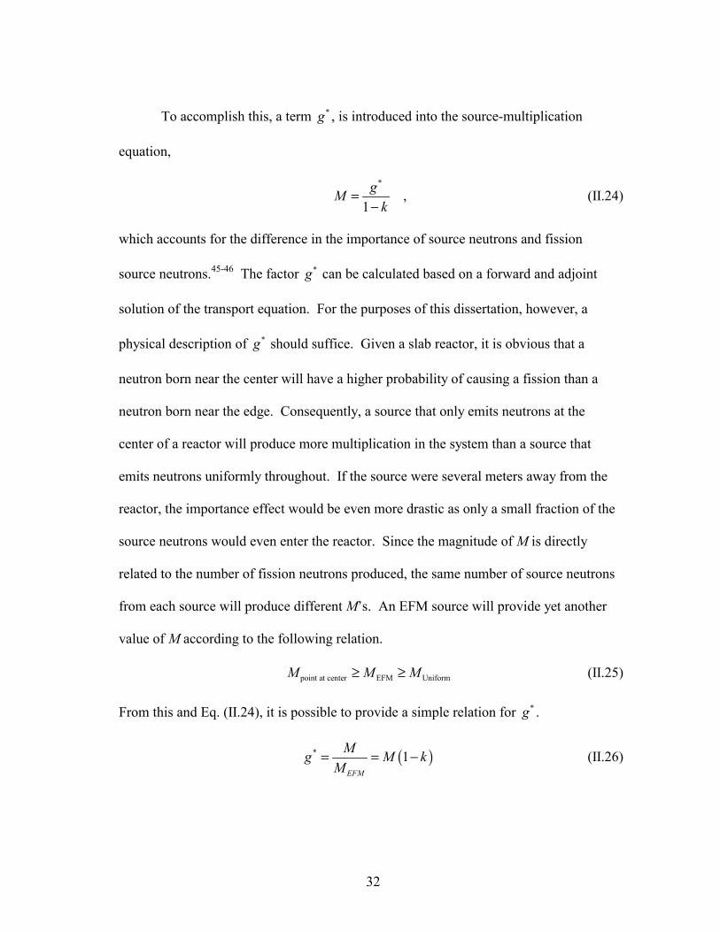
32
To accomplish this, a term *g , is introduced into the source-multiplication
equation,
*
1gM
k=
− , (II.24)
which accounts for the difference in the importance of source neutrons and fission
source neutrons.45-46 The factor *g can be calculated based on a forward and adjoint
solution of the transport equation. For the purposes of this dissertation, however, a
physical description of *g should suffice. Given a slab reactor, it is obvious that a
neutron born near the center will have a higher probability of causing a fission than a
neutron born near the edge. Consequently, a source that only emits neutrons at the
center of a reactor will produce more multiplication in the system than a source that
emits neutrons uniformly throughout. If the source were several meters away from the
reactor, the importance effect would be even more drastic as only a small fraction of the
source neutrons would even enter the reactor. Since the magnitude of M is directly
related to the number of fission neutrons produced, the same number of source neutrons
from each source will produce different M’s. An EFM source will provide yet another
value of M according to the following relation.
point at center EFM UniformM M M≥ ≥ (II.25) From this and Eq. (II.24), it is possible to provide a simple relation for *g .
( )* 1EFM
Mg M kM
= = − (II.26)

33
In the bare, spherical, uranium system studied by Spriggs, the value of *g varied as a
function of k and ranged from approximately 1.0 to 1.8 for a point source located in the
center of the assembly.
Because of the equivalence between the system subcritical prompt multiplication,
Mp, and the average chain length, L , the *g factor must also be considered when
comparing the chain-length distribution for various source configurations. For example,
to compare the chain-length distribution associated with a point source and a uniformly-
distributed source in a system operating at the same K, it is necessary to divide the
prompt system multiplication through by *g . This, in effect, allows us to compare the
chain-length distribution per EFM source (i.e., the area under each curve will be
normalized to the same value of MP).
I. Neutron Noise Analysis
The Rossi-α technique mentioned earlier is only one of many neutron noise
techniques that rely on a time-series analysis of the fluctuation in the neutron population
density. Others include the variance-to-mean, interval-distribution, zero-probability
technique etc.47-58 All of these techniques depend on quantifying the degree of
correlation associated with a stream of pulses generated by a detector. The pulses
caused by neutrons originating from a common ancestor are spaced tightly in time and
result in some number of correlated counts. Instead of describing each time-series
technique in detail, the focus here is on the Rossi-α technique, which is probably the
best known. It will be shown how the correlations arise in neutron multiplying system,

34
how they then lead to an estimate of the subcritical decay constant, α, and other global
parameters, and how the detection of correlated pairs depends on the length of the fission
chains (i.e., the chain-length distribution). It will also be shown how the detector
efficiency and a reactor’s background noise negatively effect the estimate of α.
As shown earlier, a neutron multiplying system is marked by the presence of
fission chains, whose evolution can be followed by observing the rate at which neutrons
from a common chain interact with the underlying system. The characteristic clumping
of the fission chains in time is expected to correspond to a proportionate increase in
observed events. For example, Figure 8 shows the propagation of two separate chains
over an arbitrary span of time. In this figure, the vertical lines represent the lifetimes of
the neutrons, the horizontal lines correspond to the occurrence of fission events, and the
number of tracks emerging represents the number of neutrons produced. The
terminating lines correspond to loss event whether from parasitic absorption or leakage
from the system. A fission termination would be represented by a horizontal line from
which there are no emerging lines.

35
Chain 1
Chain 2t0
t1
t1 +∆
t2
t2 +∆B C
A
Figure 8. Propagation of two prompt fission chains.
For a Rossi-α measurement to be successful, the algorithm for analyzing the
detector’s pulse stream must be able to differentiate between the pulses generated by
separate chains. In Figure 8, signals or pulses are generated whenever the branches of
the chains terminate. The events labeled A and B are detectable interactions caused by
neutrons generated in Chain 1. As such, the corresponding detector pulses provide a
single, correlated pair for the analysis. The event/pulse labeled C occurs within the same
time span as B, but it arises from a separate chain and should be recognized as an
uncorrelated, or accidental, addition to the signal. Although counts such as C cannot be
altogether eliminated, their contribution must be accounted for by knowing the average
count rate in the system. In Figure 8, the uncorrelated counts arise because the two

36
fission chains overlapped during the observed time interval. Avoiding this in an
experiment can reduce the number of accidentally correlated counts. Such a reduction
can be achieved by decreasing the rate at which the chains are initiated, by decreasing
the average chain length, or by increasing the rate at which the chains propagate.
Ignoring the uncorrelated counts for a moment, the first step towards analyzing a
detector signal requires determining the likelihood of detecting two pulses from the same
chain. Feynman, de Hoffmann, and Serber first approached this problem in 1944 during
their work on the LOPO reactor at Los Alamos.4-8 They began by assuming that a
fission event occurs at t0 and then by calculating the probability for seeing two neutrons
from that fission. After the fission, they follow the remaining pν neutrons until one
interacts in t∆ about t1. Assuming this neutron is lost from the system, only 1pν −
neutrons are then left to interact in t∆ about t2 (see Figure 9).
t0 t1 t2
∆t
A B
ν-1ν
∆t ∆t
Figure 9. Determining neutron interaction correlations.
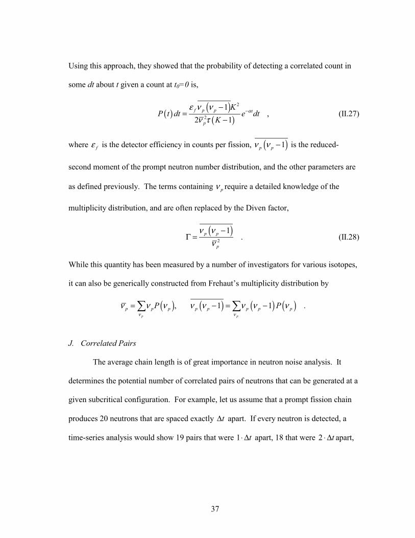
37
Using this approach, they showed that the probability of detecting a correlated count in
some dt about t given a count at t0=0 is,
( ) ( )( )
2
2
12 1f p p t
p
KP t dt e dt
Kαε ν ν
ν τ−−
=−
, (II.27)
where fε is the detector efficiency in counts per fission, ( )1p pν ν − is the reduced-
second moment of the prompt neutron number distribution, and the other parameters are
as defined previously. The terms containing pν require a detailed knowledge of the
multiplicity distribution, and are often replaced by the Diven factor,
( )
2
1p p
p
ν νν
−Γ = . (II.28)
While this quantity has been measured by a number of investigators for various isotopes,
it can also be generically constructed from Frehaut’s multiplicity distribution by
( ) ( ) ( ) ( ), 1 1p p
p p p p p p p pP Pν ν
ν ν ν ν ν ν ν ν= − = −� � .
J. Correlated Pairs
The average chain length is of great importance in neutron noise analysis. It
determines the potential number of correlated pairs of neutrons that can be generated at a
given subcritical configuration. For example, let us assume that a prompt fission chain
produces 20 neutrons that are spaced exactly t∆ apart. If every neutron is detected, a
time-series analysis would show 19 pairs that were 1 t⋅ ∆ apart, 18 that were 2 t⋅ ∆ apart,
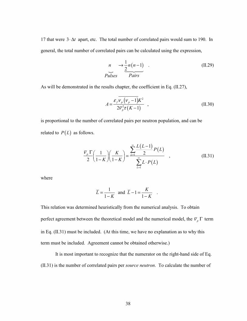
38
17 that were 3 t⋅ ∆ apart, etc. The total number of correlated pairs would sum to 190. In
general, the total number of correlated pairs can be calculated using the expression,
�
( )1 12
n n n
PairsPulses
→ −�����
. (II.29)
As will be demonstrated in the results chapter, the coefficient in Eq. (II.27),
( )
( )2
2
12 1f p p
p
KA
Kε ν ν
ν τ−
=−
, (II.30)
is proportional to the number of correlated pairs per neutron population, and can be
related to ( )P L as follows.
( ) ( )
( )1
1
11 2
2 1 1p L
L
L LP L
KK K L P L
ν∞
=∞
=
−Γ � �� � =� �� �− −� �� � ⋅
�
� , (II.31)
where
1 and 11 1
KL LK K
= − =− −
.
This relation was determined heuristically from the numerical analysis. To obtain
perfect agreement between the theoretical model and the numerical model, the pν Γ term
in Eq. (II.31) must be included. (At this time, we have no explanation as to why this
term must be included. Agreement cannot be obtained otherwise.)
It is most important to recognize that the numerator on the right-hand side of Eq.
(II.31) is the number of correlated pairs per source neutron. To calculate the number of
39
correlated pairs per neutron population, one simply divides through by the multiplication
of the system, which is the denominator on the right-hand side of Eq. (II.31).
The remaining terms contained in the Rossi-α coefficient are related to the rate at
which the correlated pairs are expected to be detected and the detector efficiency.
Because it is impossible to design an experiment in which one detects every neutron
(and hence, every correlated pair), observing the maximum number of correlated pairs
can never be achieved. Figure 8 shows a system in which only two of 12 neutrons from
the first fission chain are detected. Obviously, the detector efficiency does not change
the chain-length distribution, but it will limit the amount of information that a given
chain length provides. This will be demonstrated in the following chapter.

40

41
CHAPTER III
COMPUTATIONAL APPROACH
Because a generally applicable solution cannot be obtained analytically for
modeling the fission chain phenomena, the next best option is to examine the fission
chain process as simulated in numerical experiments. In this case, the experiments were
carried out on a computer using Monte Carlo-type simulations. The results presented
were drawn from the application of two codes that were developed to study different
dependencies of the chain-length distribution. The first code, Chain, models simple
zero-dimensional (i.e., point kinetic) systems, and the second code, MC++, models more
complex, three-dimensional systems. The following discussion focuses on the
capabilities of the two codes followed by a brief section outlining when one would
choose to use one code as opposed to the other.
A. Chain
This section begins with a description of the point-kinetic, Monte Carlo code,
Chain. To produce a chain-length distribution with this code, a user specifies the global
parameters, K and pν . Using the input global parameters, the code propagates each
chain according to a straightforward application of the previous section’s equations.
Beginning with each source neutron, the code determines a terminating event for each
neutron whether it fissions or is lost (via a parasitic absorption or a leakage). This

42
determination is accomplished by generating a random number and then determining
whether that number falls within the interval 0 to fP , where fP is defined as,
fp
KPν
= .
If the random number falls within that interval, then a fission event occurs. If, however,
the random number falls within the interval fP to 1.0, then a loss event occurs. The
event probabilities are taken to be identical for every neutron because the code assumes
that each neutron, including each source neutron, has the same distribution as an EFM
neutron. Following each fission event, another random number is generated to
determine how many neutrons were released.
The creation of each source neutron is accompanied by the creation of a new
queue that stores all of the neutrons in the chain until their terminating events have been
determined. If the terminating event is a fission event, the pν distribution is sampled,
and the resulting fission neutrons are inserted at the end of the queue. Whether the
neutron causes a fission or is lost, it is removed from its position at the front of the
queue, and the process repeats with the next neutron in the queue. When the queue is
empty, the chain has expired and its final length is registered, along with the time
interval over which the chain spawned (i.e., its duration). Because Chain is a point
model, the entire process is very efficient computationally as compared to a more
detailed simulation that tracks each neutron in energy, space, and angle. The approach
in Chain requires, at most, two random numbers per event. The first random number

43
determines the event type, and the second random number determines the number of
neutrons produced by a fission event from sampling the multiplicity distribution.
At the end of the simulation, the chain-length data, which includes the number of
neutrons in the chain, its duration, and the number of times it occurred, is written to disk.
A separate script sorts the chain length data produced by Chain into a series of
logarithmically spaced bins. The bin widths are restricted to integer increments to match
the purely integer lengths of the chains. The probability that a particular chain length
occurs is found by summing the number of chains that fall within a particular bin and
then dividing this number by the total number of chains (i.e. the number of source
neutrons tracked) and by the width of bin. The chain length associated with each
probability is taken to be the midpoint of the bin. The script with its logarithmic binning,
also works with the chain length distribution produced by MC++.
Although the logarithmic binning increases the complexity of the analysis, it is
essential because the long chains appear so infrequently. Moreover, as the chain lengths
become increasingly long, the probability of having multiple chains of the exactly the
same length decreases even faster. Increasing the bin’s width at higher values of L
increases the potential number of counts per bin by including neighboring lengths.
When the total number of counts in a given bin is divided by its width, the resulting
probability becomes the probability of seeing a chain with a range of lengths centered
about the mid-point of that bin. In addition to smoothing the estimate of observing the
long chains, this binning technique also results in the ability to observe probabilities that
can be significantly less than the inverse of the number of chains in a simulation.
44
Chain also provides a means for simultaneously running a number of neutron
noise analysis techniques while the chains are evolving. When a particular time-series
technique, such as the Rossi-α, is specified in the input file, the code also records the
time at which each event in the chain occurs. The addition of time dependent behavior
requires the generation of another random number to determine an interaction time, tevent.
Based on a user-supplied value for the neutron lifetime τ, eventt is randomly sampled
using
( )( )0 lneventt t τ ξ= + − ⋅ , (III.1) where ξ is a uniformly distributed value on the unit interval (0,1). The time of birth, 0t ,
is either the time at which a source neutron is injected into the system, or the time at
which a fission occurred that produced the current neutron. The exponential distribution
was chosen because of its close approximation to the actual time behavior of a neutrons
propagating in a single material system. All the event times in a chain are elapsed times
relative to the birth time of the initiating source neutron. In Chain, each source neutron
enters the simulation at t=0 to prevent comparison of pulses from different fission
chains. As the last neutron dies out of a chain, the event times generated by that chain
are immediately passed to the analysis routines. The event times are effectively
converted to detector pulses by applying filters that simulate the detector response.
These filters can discriminate based on event type, detector efficiency, and detector
dead-time effects. The remaining pulses from a particular chain are then analyzed, and
the analysis statistics are accumulated. The result is a very clean signal with a theoretical

45
background that does not include a contribution from overlapping chains. If the time-
series technique is the variance-to-mean, the user supplies a source rate, which is used to
space the chains out in time.
Even using the efficient techniques described, the analysis of many individual
fission chains can require large amounts of computational time if the user desires to
sample chain lengths with low probabilities of occurrence. To expedite the calculation,
Chain has been written to take advantage of multiple processor machines. Chain divides
the requested number of source neutrons evenly among the available processors. The
chain-length and noise analysis data are only collected after each processor completely
propagates its assigned source neutrons. Limiting the communication to the very start
and very end provides for an almost perfectly linear speed-up.
B. MC++
The second code presented is the production code, MC++,59-61 which has been
modified to generate chain-length distributions and analyze neutron noise signals.
MC++ is a Monte Carlo-based code designed to solve the neutron transport equation in
any arbitrary geometry. The ability to model a problem is somewhat limited by the fact
that MC++ only tracks on an Eulerian mesh. One complication encountered with this
type of mesh arises when two materials share an interface within a cell. Rather than
devising a scheme for averaging the material properties, the interface is modeled by a
plane passing through the cell. The original volumes are preserved in the approximation
along with the orientation of the materials. The algorithm allows for an indefinite
46
number of distinct materials within a cell. Even with this correction, a graphical view of
the mesh reveals that a spherical object is faceted rather than smooth. As such, most of
the test cases run involved slab type geometries since these are represented perfectly
with as few or as many cells as are desired.
Unlike Chain, a description of MC++ cannot be separated from its parallelism.
The parallel implementation was included in the original design and directly impacts the
manner in which it performs the propagation and analysis of the chains. While Chain’s
design dictates that each chain must initiate and evolve entirely on a single processor,
MC++ does not have this luxury. MC++ is built upon a generic physics framework
called Tecolote62 which is in turn based on the POOMA63,64 framework. One of the early
design considerations of these packages was to allow for highly resolved hydrodynamic
problems in an Eulerian mesh. Because these types of problems generally involve
altering the state of a physical system due to internal and external forces, the problem
decomposition for a parallel implementation was chosen such that the mesh cells
assigned to a processor corresponded to a contiguous portion of the modeled system.
While the scheme works well for hydrodynamic applications, it poses a serious
drawback for a Monte Carlo application. For these applications, having the full problem
domain split among the processors is counterintuitive as opposed to having an exact
copy of the problem on each processor as most Monte Carlo codes attempt to guarantee.
Tecolote’s prescribed decomposition scheme limits the efficiency of MC++
because the neutrons from a specific chain stream through the problem domain and may
terminate on processors other than the one from which the source neutron originated.

47
The spreading is magnified as the chains increase in length and the neutron flux begins
to distribute itself in the fundamental mode. Even in an isotropic, one-group problem
with all source neutrons starting from a single point in space, the fission neutrons will
eventually spread throughout all of the processors as they spread out in space. When a
particle moves from the mesh space of one processor to that of another, its attributes
must be communicated to the new processor, hampering the parallel efficiency. As
might be expected, the problem is exacerbated in modeled systems that are dominated by
particle streaming.
The decrease in efficiency, of MC++, is more than compensated for by its
versatility, and by the ease with which it can be customized. For example, MC++ can
model several different source configurations. This very important feature allows for a
realistic simulation since in most real systems, the initial source distribution rarely
resembles the fundamental-mode source. Most systems are driven by an intrinsic source
or an external point, both of which can have a significant impact on the chain-length
distribution. Hence, the ability to model these real-world distributions is a very
important feature of MC++.
For this reason, a user of MC++ can specify a variety of spatial distributions.
These distributions include 1) a point source at any arbitrary location internal or external
to the system, 2) a uniformly distributed source bounded within specified geometric
surfaces, or 3) a uniformly distributed source within any present fissile material, such as
an intrinsic source. The initial energy options for the source configuration include 1) a
constant value, 2) sampling from a fission spectrum, or 3) sampling from the

48
spontaneous fission spectrum for a variety of isotopes. The direction component also
provides a few sampling schemes, but the most common is a simple isotropic scheme.
Additional options can be specified for an MC++ run by setting appropriate
input parameters on the input file. For example, if the chain-length distribution is sought
during a MC++ run, each source neutron is tagged with a random number. MC++ uses
this number to identify each fission chain uniquely. As the source neutrons cause
fissions in the system, the identifier is passed along to the progeny insuring that each
neutron can be traced back to the original source neutron. If a noise analysis is required,
the tag is ignored, and instead, each source neutron is assumed to be uniformly spaced in
time according to the specified source strength. The tag is not required in this case
because each source neutron is associated with a unique “birth time” which simulates the
time it appeared in the system relative to the other source neutrons, and a “track time”
which stores the amount of time the neutron exists until it leaves the system. The first
source neutron on the master processor begins at time, t=0 and the last neutron on the
last processor will be set to t=tlast where
10
Number of Total Sources
sec
last
eff
tnS � �
� �� �
� . (III.2)
The source strength, Seff, may be specified in the input file or selected from a store of
spontaneous fission decay constants for a variety of isotopes. Naturally, the two run
types are not mutually exclusive and result in neutrons with unique identifiers and the
appropriate birth times.
49
Once the neutrons have been placed within the simulation environment, they and
any fission neutrons they produce will either leave the current cell, leak from the
problem, or collide with the cell material during each transport cycle in MC++. A
transport cycle involves determining which of the events occurs for each of the neutrons
that are active in the system. This decision is made after comparing the distances along
the particle’s flight path to the nearest cell boundary, material interface plane, and
collision site. The shortest distance determines the event chosen. If the collision
distance happens to be the shortest, the incident neutron is either scattered, parasitically
absorbed, or absorbed in a reaction leading to fission. In the first case, the neutron has
its energy and angle appropriately adjusted and continues its flight. The second case
results in a the neutron being completely removed from the system unless there is the
possibility for an (n,xn) reaction. The fission event terminates the incident neutron and
adds to the neutron population the number of neutrons sampled from the neutron number
distribution (i.e., which has been specified to be the modified version of Frehaut’s
distribution discussed in an earlier chapter).
To remain faithful to the physics of the simulation, all the collisions are treated in
an analog Monte Carlo fashion. As such, there are currently no variance reduction
techniques employed to improve statistics. However, given the nature of the problem, it
is not yet clear how such techniques could be applied while preserving the underlying
stochastic phenomena.
Consequently, Chain requires system-averaged parameters such as K , pν , and τ,
but in MC++, the collision physics are based on the nuclear cross sections requested in
50
the input file. (For the current version of MC++ the cross sections must be in a multi-
group format as the continuous energy cross sections have not been fully implemented.)
During the problem setup stage, the total microscopic cross section for each material is
computed from the constituent isotopes. The probability of interaction per unit path
length is found by multiplying the microscopic cross section by the material density
stored in the local mesh cell. The particular isotope chosen is based on a random
number and the relative contribution of each of the individual isotopes to the total cross
section. Another step required during the setup is to construct a Frehaut distribution table
for each energy group’s pν for each isotope.
The computational process is slightly different and more complicated if the user
desires to produce a chain length distribution for a particular system. In this case, the
unique identifier of the source neutron is passed to each neutron that it produces from
fission or inelastic scattering. After each event that produces neutrons, the counter
associated with the initiating neutron’s identifier is incremented. At the end of each
transport sweep, the list of chain lengths is passed through. Of course, as nature would
have it, as K nears 1.0, the probability for seeing nearly infinite-length chains becomes
more distinct. However, the MC++ simulation is constrained by the memory available
on the executing host. For this reason, a maximum chain length is specified. Any chain
that exceeds this value is recorded, and the currently present members of this chain are
removed from the simulation. This process has been separated from the noise analysis
(although they can be run simultaneously) because of the large amount of

51
communication required after each sweep for the code to know exactly how many
neutrons are still “alive” in each chain.
C. Analytic Cross Sections
An important goal of this work is to compare the results from the zero-
dimensional and three-dimensional codes. Given the obvious difference in their
handling of spatial effects, a valid comparison of results from two such codes hinges on
the ability to construct problems that are as physically similar as possible. This objective
implies constructing a three-dimensional system for MC++ that has identical system
parameters to those supplied to Chain. Of the parameters of interest, the chain-length
distribution and the *g calculation are sensitive to differences in the system’s K. In
Chain, this value is supplied directly, but in MC++, it must be computed.
As is the case with any Monte Carlo code, MC++’s determination of the neutron
multiplication factor is actually dependent on many individual collisions and neutron
tracks occurring over a series of independent transport cycles. The energy and angular
dependence of the solution appear as a result of the nuclear data used to sample the
collisions. The data also determines the appropriate interpretation of the multiplication
factor. If the data provides promptν , the factor is the prompt multiplication factor, K,
whereas totalν yields the traditional k. The location of materials within the problem and
the density of the collisions determine the spatial dependence. As might be expected,
the sampling of the individual events leads to an estimate for the neutron multiplication
factor that has an associated uncertainty whose magnitude is determined by the number
52
of histories compiled. Similar to reducing the variance in the multiplicity, using a single
energy group reduces the variance in a k-eigenvalue solution, but reducing the variance
associated with the spatial effects is considerably harder. As such, it would be difficult,
ad hoc, to construct a problem that has a K exact to many decimal places.
For this reason, the reference problems have been constructed according to the
specifications that accompany a set of analytical cross sections.65 The analytical cross
sections were specifically formulated for use with analytical benchmark problems to be
solved using deterministic and stochastic transport codes that compute static k-
eigenvalues. Based on analytic solutions of the transport equation, these cross sections
make it possible to compare the zero-dimensional and three-dimensional codes. In the
simple geometries for which they are valid, these cross sections provide k-eigenvalues of
exactly 1.00000. These problems include both bare and water-reflected systems
comprised of infinite cylinders, spheres, and right circular cylinders. Although MC++ is
capable of modeling any of these geometries, the infinite slab case has been selected
because it can be exactly modeled in the computational mesh available in MC++. The
curved surfaces associated with the other geometries require a large number of mesh
cells to reduce the effects cause by the resulting faceted surfaces. The majority of the
MC++ runs were done with cross sections from the mock plutonium set with the pν
adjusted as necessary to obtain a range of analytic K’s less than 1.0. The plutonium data
appears in Table IV.

53
TABLE IV
Analytic cross section set corresponding to Pu.
ν fΣ cΣ sΣ tΣ
3.24 0.0816 0.019584 0.225216 0.8264
D. Noise Analysis in MC++
The neutron sources are divided into a series of batches. This option has been
adopted to avoid memory limitations encountered when following millions of neutrons
through the simulation. By batching, the limitation shifts to how long it takes to run a
sufficient number of batches to acquire the required statistical uncertainties. To
faithfully reproduce the signal in a detector, the source neutrons in a batch are randomly
spaced in time according to the source rate.
When there are no longer any neutrons in the simulation, the processors
communicate their pulses to the master processor (Node 0). The pulses represent the
simulated detector response to the neutron events that occurred on a processor, and they
are stored as a list of times at which the detected events occurred. The events
themselves may represent fissions, captures, or escapes depending on the simulated
detector type. The master processor sorts the pulses in ascending order in time. It then
divides the total number of pulses by the number of processors in the simulation. What
happens next depends on the type of noise analysis technique desired. Even in an actual
Rossi-α experiment, it is impossible to know beforehand exactly when each chain begins

54
and ends. If two or more chains happen to overlap, there is no ideal way to differentiate
the beginning of a particular chain. For this reason, each processor receives a nearly
complete copy of the pulse stream from the master processor. The only difference is that
each processor receives a chain that begins farther along the sequence. In this way, all
the processors have access to the downstream pulses required to construct the most
possible correlated pairs. This elaborate scheme would not be necessary for a simulation
of a pulsed neutron experiment since the pulses are only compared against their
neighbor. Splitting the pulses across the N-processors would only result in the loss of N-
1 pulse comparisons.
E. Handling the Background Noise
Although the conglomeration of each chain’s contribution into a single pulse
stream is identical to what happens in actual experiments, it adds another element of
complexity to interpreting the signal. The resulting pulse stream contains a potentially
high number of uncorrelated pulses that arise from comparison of pulses from separate
chains. Fortunately, this background noise can be handled by MC++ in the same fashion
that it is handled in an actual experiment. In both cases, its magnitude can be found by
taking the total number of counts recorded in the detector and dividing by the total time
spent counting.
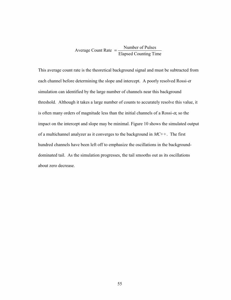
55
Number of PulsesAverage Count Rate Elapsed Counting Time
=
This average count rate is the theoretical background signal and must be subtracted from
each channel before determining the slope and intercept. A poorly resolved Rossi-α
simulation can identified by the large number of channels near this background
threshold. Although it takes a large number of counts to accurately resolve this value, it
is often many orders of magnitude less than the initial channels of a Rossi-α, so the
impact on the intercept and slope may be minimal. Figure 10 shows the simulated output
of a multichannel analyzer as it converges to the background in MC++. The first
hundred channels have been left off to emphasize the oscillations in the background-
dominated tail. As the simulation progresses, the tail smooths out as its oscillations
about zero decrease.

56
Time [sec]
5.0e-6 1.0e-5 1.5e-5 2.0e-5
Cou
nt P
roba
bilit
y [1
/sec
]
-1e+7
0
1e+7
2e+7
3e+7
4e+7
5e+7
6e+7
7e+7
6 M26 M 65 M 133 M
Theoretical Background
Figure 10. Resolving the background noise threshold.

57
CHAPTER IV
NUMERICAL RESULTS
The purpose of this chapter is to present the results of some chain-length
distribution calculations performed by Chain and MC++ for a variety of prompt neutron
multiplication factors and source configurations. However, to lend credence to the
results, the point model code is validated by showing that the chain-length distribution
produced by Chain yields the correct subcritical prompt multiplication, Mp, for a
specified prompt multiplication constant, K. Validation of the more complex three-
dimensional code, MC++, will be performed by making a direct comparison to results
from the point model code, Chain. Following this validation, it will be shown how the
contribution of the longest chain lengths becomes negligible when estimating the
subcritical prompt multiplication and when performing neutron noise analysis. A series
of chain-length distributions have been generated to identify the factors that have the
greatest effect on the distributions. After illustrating the general form and sensitivities of
the chain-length distribution to the most important factors, the critical role that the
fission chains play in common neutron noise analysis techniques is examined. This
chapter concludes by showing how MC++ reproduces the multiple prompt decay modes
that arise because of harmonic effects in highly subcritical systems and because of
spatial effects in finite multi-region subcritical systems. It will be shown that detailed
information regarding the fission chains is an essential key to understanding and
predicting the neutron noise signal that might be observed in subcritical experiments.

58
A. Code Validation
Although MC++ has been benchmarked against the widely used Monte Carlo
code, MCNP, the comparisons have been limited to static k and α eigenvalue problems.60
The current version of MCNP does not follow individual fission chains and, as such,
precludes any direct comparison of the chain-length distribution calculated by the two
codes. Nevertheless, the chain propagation algorithms in MC++ have been
benchmarked against the chain-length distribution calculated by the zero-dimensional
code, Chain. Furthermore, the analytic cross sections have been used to verify the
particle interaction physics in MC++ with regards to k-eigenvalue calculations.
Because Chain is a point model, it is assumed that the source neutrons are
distributed as an EFM source, and consequently, they have a common probability for
inducing fission. If one follows the branching chains shown in Figure 6, it is possible to
construct a family of branches that result in a single chain length. Several of the shorter
paths have been combined with the results from Frehaut’s multiplicity distribution to
construct an analytical benchmark for problems with known chain-length distributions.
Tables V and VI show that the chain-length distributions generated by Chain are
accurate regardless of the initial K or pν .
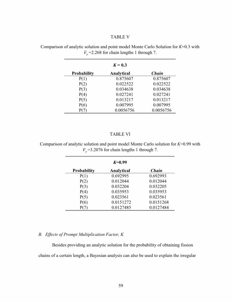
59
TABLE V
Comparison of analytic solution and point model Monte Carlo Solution for K=0.3 with pν =2.268 for chain lengths 1 through 7.
K = 0.3
Probability Analytical Chain P(1) 0.875607 0.875607 P(2) 0.022522 0.022522 P(3) 0.034638 0.034638 P(4) 0.027241 0.027241 P(5) 0.013217 0.013217 P(6) 0.007995 0.007995 P(7) 0.0056756 0.0056756
TABLE VI
Comparison of analytic solution and point model Monte Carlo solution for K=0.99 with pν =3.2076 for chain lengths 1 through 7.
K=0.99
Probability Analytical Chain P(1) 0.692995 0.692993 P(2) 0.012044 0.012044 P(3) 0.032204 0.032205 P(4) 0.035953 0.035953 P(5) 0.023561 0.023561 P(6) 0.0151272 0.0151268 P(7) 0.0127485 0.0127484
B. Effects of Prompt Multiplication Factor, K
Besides providing an analytic solution for the probability of obtaining fission
chains of a certain length, a Bayesian analysis can also be used to explain the irregular

60
behavior observed in the chain-length distributions plotted in Figure 11. In this figure,
plots are shown for the chain-length distributions associated with a variety of K and
2.268pν = . Although the portion of the distribution associated with the shorter chain
lengths appears discontinuous and inconsistent with the remainder of the distribution, the
probabilities match exactly with the results predicted by the Bayesian analysis. As
predicted, the most probable chain length is 1.0, which corresponds to a source neutron
that does not produce any subsequent fission neutrons. Similarly, the dip at L=2 is
expected since a chain length of two can only occur if the source neutron undergoes a
fission in which only a single neutron is released. According to Frehaut’s multiplicity
distribution, the likelihood of this happening is slightly less than a fission event in which
2 or more neutrons are released.
The tails of the distributions are not so easy to describe analytically since the
potential number of paths becomes very large, making an analytic solution derived from
Bayesian statistics impractical. Nevertheless, there is some confidence that certain
characteristics of the chain-length distribution can be inferred without the benefit of an
analytic solution. For example, it is noteworthy that as K increases, each distribution
exhibits an asymptotic behavior at the longer chain lengths. Although the distribution
does not indicate the presence of an absolute maximum chain length, it does indicate that
that chain lengths farther along the asymptotic tail are highly improbable. For K=0.3,
the probability of seeing a chain length of 105 neutrons is 131 10 .−⋅ For K=0.999, this
same probability is associated with a much longer chain length of approximately 73 10⋅
neutrons. Although the probabilities for very long chain lengths are difficult to

61
determine accurately because of their rarity, this rarity corresponds to a vanishingly
small effect on the system performance.
Chain Length
100 101 102 103 104 105 106 107 108
P(L)
100
10-2
10-4
10-6
10-8
10-10
10-12
10-14
K=0.3 K=0.5 K=0.7 K=0.9 K=0.99 K=0.999 Galton-Watson
P(L) = 0.29 L-1.5
Figure 11. Chain-length distributions for select values of K.
Figure 11 also shows that as K increases, the probability for observing all chains
with lengths greater than 1 increases. As expected, as 1.0K → , the average chain
length approaches infinity. The reason why the probability of observing a chain length
of L=1 decreases as K increases can be easily seen from the analytical solution for ( )1P ,

62
( ) 01 1p p
K KP Pν ν
� �= − +� �� �� �
.
As K increases, it is also apparent from the above Figure 11 that larger portions
of each distributions follow the Galton-Watson approximation, which predicts that the
probability of obtaining a chain of length L varies as,
( ) 1.5P L C L−= ⋅ .
The particular solution of the Galton-Watson problem corresponds to the case in which
K=1.00, and implies that a prompt-critical system will have a finite probability
generating a chain of nearly infinite length. As observed in the numerical solutions, the
quantity C in this equation is slightly dependent on K. However, to a first
approximation, C can be taken to be approximately equal to 0.29.
Unless otherwise noted, the figures in this section are based on results from a
series of Chain runs that are described in Table VII. The decrease in the number of
source neutrons was an unavoidable consequence of the 6-hour runlimit imposed on the
ASCI Blue Mountain computer at Los Alamos National Laboratory. In Chain, the
majority of the computation time is expended calling the random number function.
Consequently, a limit on the total computation time directly limits the total number of
neutrons that can be tracked and not the number in the source itself. With this in mind,
each run was designed to last 5 hours running on 1008 processors except for the case
with K=0.5 in which the number of processors was doubled. The 5-hour limit was
chosen because the queuing system on the machine terminates any process that exceeds
the current 6-hour limit. The limitation on the runtime resulted in chain-length

63
distributions at higher K that are not as thoroughly sampled as are those at lower values
of K. The lack of resolution in the chain-length distribution is readily apparent in the
increasing uncertainty in the estimate for the subcritical prompt multiplication. Even
with the just-noted limitations, all of the runs were able to follow a large number of
chains revealing much of the structure in the low-probability tail. Later in this chapter,
the chain-length distributions resulting from these Chain runs will be presented as plots
labeled as EFM.
TABLE VII
Multiplication obtained during various Chain simulations.
K #Sources Tracked Analytic M Computed M 0.3 1.08e13 1.54e13 1.4285714 1.428571723 0.5 1.50e13 3.00e13 2.0 2.000000157 0.7 5.00e12 1.66e13 3. 333 3.333334098 0.9 1.66e12 1.66e13 10.0 10.00001108 0.99 1.66e11 1.66e13 100.0 100.0016458 0.999 1.66e10 1.66e13 1000.0 1000.135725
As mentioned in the previous section, the chain-length distribution is directly
related to the subcritical prompt multiplication of the system. Figure 12 shows that the
integral of the chain-length distribution asymptotically becomes equal to pM of the
system. Because of the binning technique used, which was described in a previous
chapter, the integration to obtain the integral chain length was performed according to
Eq. (IV.1).

64
0
NumBins
p i i ii
M P L BinWidth=
= ⋅ ⋅� (IV.1)
Moreover, the subcritical prompt multiplication predicted by the above integral chain
length can be compared to the subcritical prompt multiplication computed analytically
from the user supplied K in order to verify the algorithm performance. For this reason,
the K values were chosen such that their corresponding M’s are whole integers that are
easily identifiable on the plots presented in Figure 12.
The plots in Figure 12 also reveal an interesting property related to the
importance of the integral contributions of the chain lengths located along the
asymptotic tail. Without exception, each of the curves reached the final subcritical
prompt multiplication value (to a first approximation) without inclusion of the last
decade or so of lengths in the integral. From this observation, it can be concluded that
although the longest chains considered had lots of neutrons in them, their presence does
not significantly effect the multiplication of the system since they so rarely occur. In
addition, inclusion of even longer chain lengths will have negligibly small effects on the
computed subcritical prompt multiplication.

65
Chain Length
100 101 102 103 104 105 106 107 108
Inte
gral
Pro
mpt
Sub
criti
cal M
ultip
licat
ion
1
10
100
1000
K=0.5 K=0.9K=0.99K=0.999
Figure 12. Integral of the chain-length distribution showing its relationship to the
subcritical prompt multiplication, Mp.
The lack of importance of the longest chains to these calculations is also apparent
in Figure 13, which provides another way to look at the contribution of the longest chain
lengths, i.e., those located in the tail of the chain-length distribution. Instead of looking
at the integral contribution of all of the chains, in Figure 13 the chain length, L, has been
multiplied by the probability of its occurrence. In this figure, it is possible to readily see
which chains contribute the most to the subcritical prompt multiplication process. There
are two conclusions that can be drawn from Figure 13. First, the vast majority of the

66
subcritical prompt multiplication of a system is produced by small-to-intermediate
length chains that occur with relatively high probability. And, in accordance with
previous conclusion, the longest chains in the distribution simply do not affect the
subcritical prompt multiplication due to their rarity. Although the chain lengths at
K=0.99 extend past a length of 105 neutrons, ignoring the contribution of the chains past
a length of 104 neutrons would only result in a 2% error in the final estimate of the
subcritical prompt multiplication.
Chain Length
100 101 102 103 104 105
Diff
eren
tial S
ubcr
itica
l Pro
mpt
Mul
tiplic
atio
n
0.00
0.02
0.04
0.06
0.08
0.10
0.12
0.14
0.16
0.18
K=0.3K=0.7K=0.99
Figure 13. Differential subcritical prompt multiplication contribution of chain lengths
L>1 for various K.

67
C. Effects of Multiplicity Distribution
As briefly mentioned earlier, the type of neutron multiplicity employed to
generate the fission chains has a significant impact on the chain-length distribution. The
influence is most noticeable for the shorter chain lengths because of the limited number
of paths a chain may take. Any perturbations at either end of the chain-length
distribution must be compensated elsewhere to keep the subcritical prompt
multiplication constant. Thus, a non-physical representation of the neutron multiplicity
can have an unusual effect, the magnitude of which depends on the value of K. In Figure
14, one chain-length distribution was computed using a binary distribution (i.e., either 2
or 3 neutrons are released per fission as assumed in analog MCNP), and the other
distribution was computed using the more realistic Frehaut distribution. For both cases,
K=0.5 and 2.268pν = . The former chain-length distribution shows some initial
oscillations for the chain lengths around 7-10 neutrons, which are quickly damped.
Because the prompt multiplication constant, K, of the system was specified to be
identical in both cases, the area under the two curves must also be identical.
Consequently, an increase in the chain length probabilities at one end of the chain-length
distribution must be offset by a decrease in the probabilities at the opposite end. In
conclusion, when simulating the evolution of fission chains using Monte Carlo
techniques, one should strive to model the neutron multiplicity as accurately as possible
in order to avoid skewing the resulting chain-length distribution.
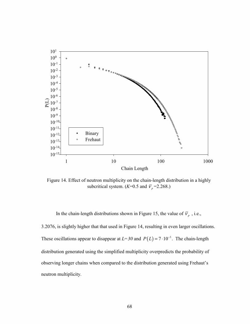
68
Chain Length1 10 100 1000
P(L)
10-1510-1410-1310-1210-1110-1010-910-810-710-610-510-410-310-210-1100101
BinaryFrehaut
Figure 14. Effect of neutron multiplicity on the chain-length distribution in a highly
subcritical system. (K=0.5 and pν =2.268.)
In the chain-length distributions shown in Figure 15, the value of pν , i.e.,
3.2076, is slightly higher that that used in Figure 14, resulting in even larger oscillations.
These oscillations appear to disappear at L=30 and ( ) 37 10P L −= ⋅ . The chain-length
distribution generated using the simplified multiplicity overpredicts the probability of
observing longer chains when compared to the distribution generated using Frehaut’s
neutron multiplicity.

69
Chain Length1 10 100 1000
P(L)
10-1510-1410-1310-1210-1110-1010-910-810-710-610-510-410-310-210-1100101
BinaryFrehaut
Figure 15. Effect of neutron multiplicity on the chain-length distribution in a highly
subcritical system. (K=0.5 and pν =3.2076)
When the value of K is increased, the effect on the chain-length distribution
appears to be minimal though it is nevertheless observable (see Figure 16). In this case,
the distribution appears to overpredict the mid-range chain lengths while it under
predicts the longest values. Similar to the previous example that used the lower value of
pν , the oscillations die out quickly.
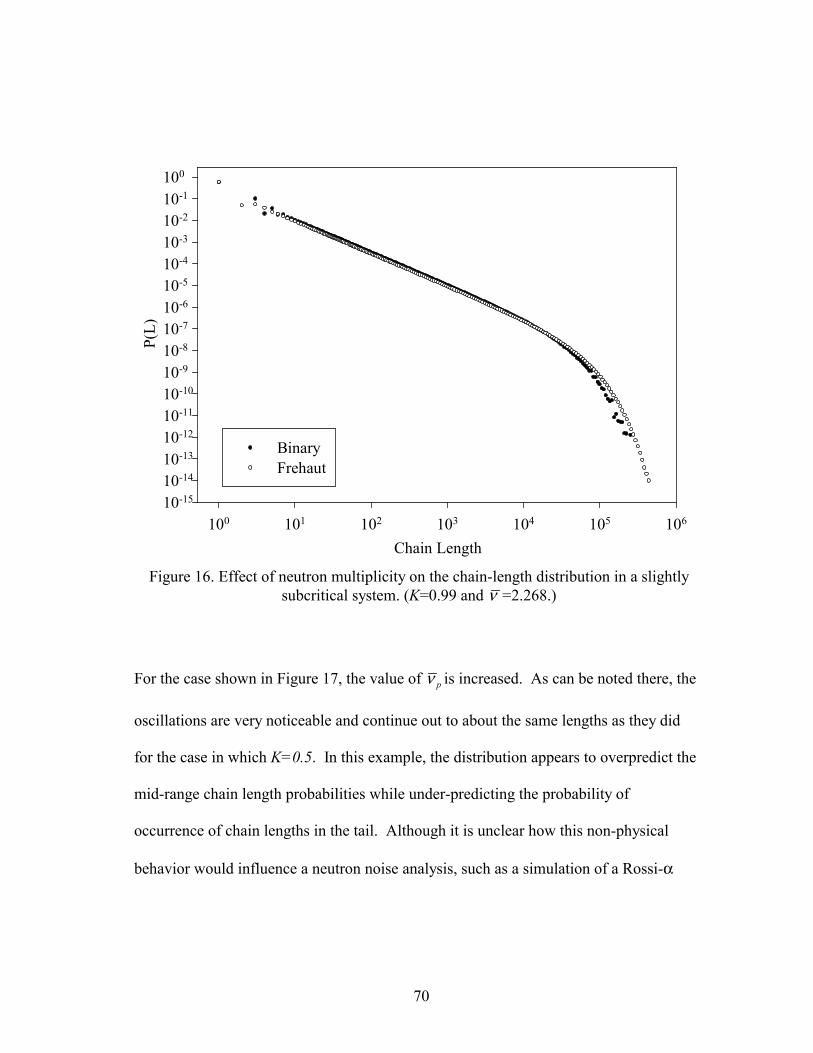
70
Chain Length100 101 102 103 104 105 106
P(L)
10-1510-1410-1310-1210-1110-1010-910-810-710-610-510-410-310-210-1100
BinaryFrehaut
Figure 16. Effect of neutron multiplicity on the chain-length distribution in a slightly
subcritical system. (K=0.99 and ν =2.268.)
For the case shown in Figure 17, the value of pν is increased. As can be noted there, the
oscillations are very noticeable and continue out to about the same lengths as they did
for the case in which K=0.5. In this example, the distribution appears to overpredict the
mid-range chain length probabilities while under-predicting the probability of
occurrence of chain lengths in the tail. Although it is unclear how this non-physical
behavior would influence a neutron noise analysis, such as a simulation of a Rossi-α

71
measurement, its alteration of the fission chain length variance may have a noticeable
effect in techniques such as the Feynman’s variance-to-mean method.
Chain Length100 101 102 103 104 105 106
P(L)
10-1510-1410-1310-1210-1110-1010-910-810-710-610-510-410-310-210-1100101
BinaryFrehaut
Figure 17. Effect of neutron multiplicity on the chain-length distribution in a slightly
subcritical system. (K=0.99 and pν =3.2076)
D. Effects of Average Prompt Multiplicity, pν
In addition to the effect on the chain-length distribution resulting from the
neutron multiplicity, the magnitude of pν has a substantial impact on the chain-length
distribution curve. In Figure 18, the resulting chain-length distributions are compared

72
for a K=0.5 with pν equal to 2.268 and 3.2076. As expected, the fP for each EFM
neutron decreases with increasing pν . That is,
fp
KPν
= .
Because the probability of a neutron loss varies as ( )1 fP− , it then follows that the
probability of observing chains with lengths of 1 (L=1) will increase with an increase in
pν . Furthermore, while P(1) increases, the numerical simulation simultaneously
predicts that the probability of seeing short chains (i.e., 2, 3, 4, etc.) decreases as
pν increases. The longer chains are more likely in this case because the number of
neutrons per fission is increasing resulting in slightly longer chains. When the chain-
length distributions for the two different values of pν are compared, it is noted that for
the case with the higher value of pν the probability of spawning chains with long lengths
is higher than for the case with the lower value of pν . This increase must occur in order
to offset the differences in the chain-length distribution at low values of L (i.e., the areas
under both curves are identical). A more physical way of expressing this idea is to see
that in both cases the total number of fissions is roughly constant. For a fixed value of
K, a higher pν results in more neutrons being released per fissions, but this is offset by
the decrease in the probability that they will cause other fissions.

73
Chain Length
1 10 100 1000
P(L)
10-15
10-14
10-13
10-12
10-11
10-10
10-9
10-8
10-7
10-6
10-5
10-4
10-3
10-2
10-1
100
101
νp = 2.268νp = 3.2076
Figure 18. pν effects on the chain-length distribution at K=0.5.
When cases with a higher K and the two values of pν are considered, it reveals a
noteworthy trend in the chain-length distributions at the intermediate lengths (see Figure
19). Keeping in mind that the prompt multiplication, K, is identical for both cases, one
might expect that the higher value of pν would show higher probabilities for all but the
shortest chain lengths. However, Figure 19 shows that for the majority of the chain
lengths, the higher pν actually results in lower probability of occurrence values, ( )P L ,
except near the tail of the distribution at large chain lengths. In this case, the

74
probabilities of occurrence for the chain lengths in the tail of the distributions are
expected to have discernable impacts on the subcritical prompt multiplication
calculations.
Chain Length
100 101 102 103 104 105 106
P(L)
10-15
10-14
10-13
10-12
10-11
10-10
10-9
10-8
10-7
10-6
10-5
10-4
10-3
10-2
10-1
100
101
νp = 2.268
νp = 3.2076
Figure 19. pν effects on the chain-length distribution at K=0.99.
Although, it might not be clear from Figure 19 how the tail contribution could be
sufficient to guarantee the same subcritical prompt multiplication, the similarity becomes
evident in Figure 20. The integral of the distributions is shown there, and it
demonstrates that the distribution corresponding to 2.268pν = reaches its asymptotic

75
value sooner than the distribution corresponding to 3.2076pν = . In this representation,
it can be concluded that it is essential to sample the entire chain-length distribution,
including the very long chain length values to insure the accuracy of the parameters of
interest.
Chain Length
100 101 102 103 104 105 106
Inte
gral
Mul
tiplic
atio
n
1
10
100
νp = 2.268
νp = 3.2076
Figure 20. pν effects on the integral subcritical prompt multiplication.
E. Effects of the Initial Source
The data appearing in the preceding figures were all produced using Chain,
which is a zero-dimensional model and, as such, is unable to predict spatial effects.

76
Nevertheless, spatial effects are always present in any real experiment, and their
inclusion is indispensable to accurate computational simulations. In order to study
spatial effects on the chain-length distribution, the three-dimensional Monte Carlo code,
MC++, described in Chapter IV was used. In this section, it is shown how the chain-
length distribution changes as a function of the source configuration that drives a multi-
dimensional system. Three different source configurations were studied: 1) a point
source, 2) a uniformly-distributed, volumetric source, and 3) an equivalent fundamental-
mode (EFM) source. The results that are associated with the EFM source generally have
smaller statistical uncertainties than the results for the volumetric and point sources since
it was possible to sample a greater number of particles in a fixed amount of time when
the simpler, EFM model was used. Each of the cases presented in this section was run
for a homogeneous, slab reactor. A set of analytical, one-energy group, cross sections
was adjusted to match the K for the slab to that used in Chain.
Figure 21, the first in this series, shows the results for a K=0.7 and focuses on a
representative portion of the chain-length distribution. This plot shows the ( )P L
distributions for a point source, EFM source and a volumetric source. The ( )P L
corresponding to the point source lies above the other two, which is expected since the
source neutrons are born at the center of the slab, and, as such, have a higher probability
for causing a fission before leaking from the system. The next highest line corresponds
to the EFM distribution. Because the fundamental mode in a slab reactor resembles a
chopped cosine function, most of the EFM source neutrons are born near the center of
the reactor, but there are a significant number of births near the edge of the slab. The

77
lowest curve belongs to the volumetric source which has even fewer source neutrons
started near the center of the slab and more born near the edges.
Chain Length10 100
P(L)
10-5
10-4
10-3
10-2
EFM VolumetricPoint
Figure 21. Spatial effects on the chain-length distribution caused by the source
configuration. (K=0.7)
When K is increased to 0.99, the same relative positions of the three chain-length
distribution are observed (see Figure 22).

78
Chain Length101 102 103
P(L)
10-5
10-4
10-3
10-2
EFMVolumetricPoint
Figure 22. Spatial effects on the chain-length distribution caused by the source
configuration (K=0.99)
Unlike the results presented in the previous sections that demonstrated the effects
on the chain-length distribution associated with changes in pν and the neutron
multiplicity, the subcritical prompt multiplication of the slab is not identical for the three
different source configurations. This difference is readily apparent when one integrates
the chain-length distribution produced by the three source configurations (see Figure
23). As can be seen there, each source distribution leads to a different asymptotic value
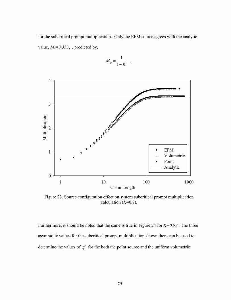
79
for the subcritical prompt multiplication. Only the EFM source agrees with the analytic
value, Mp=3.333… predicted by,
11pM
K=
− .
Chain Length1 10 100 1000
Mul
tiplic
atio
n
0
1
2
3
4
EFMVolumetricPointAnalytic
Figure 23. Source configuration effect on system subcritical prompt multiplication
calculation (K=0.7).
Furthermore, it should be noted that the same is true in Figure 24 for K=0.99. The three
asymptotic values for the subcritical prompt multiplication shown there can be used to
determine the values of *g for the both the point source and the uniform volumetric

80
source. As long as the actual prompt multiplication factor, K, is known, this technique
can be used to determine *g from the measured multiplication of the system, M.
Chain Length100 101 102 103 104 105 106
Mul
tiplic
atio
n
1
10
100
EFMVolumetricPointAnalytic
Figure 24. Source configuration effect on the system multiplication calculation (K=0.99).
F. Effect on Noise Analysis
As mentioned in the previous chapter, a Rossi-α analysis can provide a great deal
of information about the neutronic characteristics of a multiplying system. Because the
Rossi-α technique is based on the detection of correlated pairs of counts, it is of interest
to determine the maximum number of correlated pairs that can be expected at a certain

81
value of K. This number can be readily calculated from the chain-length distribution as
follows.
( )0
1Num Pairs 12
NumBins
i i i ii
P L L BinWidth=
= ⋅ − ⋅� (IV.2)
Figure 25 shows the integral contribution of different chain lengths to the total number
of correlated of pairs for several values of K. The maximum value of attained by each
curve corresponds to the actual number of pairs expected per source neutron. However,
when performing a Rossi-α experiment, the quantity measured is the number of
correlated pairs per neutron population. Consequently, the expected number of pairs is
higher than the value from Eq. (IV.2) by a factor of Mp. Further, if one takes the
asymptotic value for the number of correlated pairs shown in Figure 25 and multiplies
this by the effective source rate driving the system (i.e. the fixed source plus the delayed
neutron source), the maximum number of correlated pairs expected per second can be
obtained. Similarly to the previous results, it is observed that the contribution from the
longest chain lengths is minimal due to their low probability of occurrence.

82
Chain Length
100 101 102 103 104 105 106 107 108
Inte
gral
Exp
ecte
d C
orre
late
d Pa
irs p
er E
FM S
ourc
e
10-2
10-1
100
101
102
103
104
105
106
107
108
109
1010
K=0.3K=0.5K=0.7K=0.9K=0.99K=0.999
Figure 25. Theoretical maximum number of correlated pairs of neutrons per source
neutron from an EFM source.
Because the plots shown in Figure 25 were generated with a numerical
simulation, several factors are not accounted for that would affect an actual experimental
measurement. When Chain and MC++ tally the neutrons that appear in each chain, the
neutrons are counted regardless of their final location, energy, or type of terminating
event. In practice, detectors are generally more sensitive to certain types of events or to
prescribed energy ranges and their responses are always affected by their location
relative to the configuration of the neutron multiplying system. From an experimental

83
viewpoint, it is always desirable to use a detection system that does not significantly
alter the fundamental parameters that are to be measured. For example, placing a plastic
scintillation detector in the middle of a small, fast reactor, such as Godiva, would
probably result in a significant change in the neutron lifetime. Hence, a measured
lifetime obtained by a Rossi-α measurement would not be characteristic of the lifetime
in the same system without the detector. Therefore, experiments should be designed and
executed in ways that do not unduly influence the natural evolution of fission chain
propagation.
Although it is feasible to locate a detector such that it does not induce an
unwanted perturbation in the chain-length distribution, location and other factors
invariably affect the detector’s overall efficiency, which is the efficiency that appears in
the analysis equations. These efficiency considerations affect the portion of the fission
chain events in the neutron multiplying system that are sampled. Even under the best of
circumstances, efficiency considerations must be dealt with for real systems along with
their potentially drastic effects on the values derived from a neutron noise analysis. To
demonstrate this necessity, the Chain code’s estimate for the number of correlated pairs
per source neutron can be considered again this time when certain events are ignored.
The number of expected pairs drops significantly simply by limiting the detector’s
sensitivity to those neutrons that leak or are parasitically absorbed (~40%). In the real
world, a large loss in the number of detectable pulses might need to be offset in some
manner such as by using more detectors.

84
Chain Length
100 101 102 103 104 105 106 107 108
Inte
gral
Exp
ecte
d C
orre
late
d Pa
irs p
er E
FM S
ourc
e
10-2
10-1
100
101
102
103
104
105
106
107
108
109
K=0.3K=0.5K=0.7K=0.9K=0.99K=0.9991 pair/source
Figure 26. Expected number of correlated pairs from a capture detector with an
efficiency of 100% for various K.
The horizontal line in Figure 26 shows the level at which the total number of
correlated pairs produced per source neutron is less than 1.0. This level is also shown in
Figure 27 with the detector efficiency taken into account. In making Figure 27, the
efficiency has been arbitrarily set to 10%, and this value reduces the number of expected
correlated pairs by a factor of 100. This sensitivity to the detector efficiency arises
because the chain length is squared in Eq. (IV.2). Even with these considerations, it is

85
clear that the higher K values will still provide a substantial number of correlated pairs
per source neutron.
Chain Length100 101 102 103 104 105 106 107 108
Inte
gral
Exp
ecte
d C
orre
late
d Pa
irs p
er E
FM S
ourc
e
10-4
10-3
10-2
10-1
100
101
102
103
104
105
106
107
108
K=0.3K=0.5K=0.7K=0.9K=0.99K=0.9991 pair/source
Figure 27. Expected number correlated pairs using a capture detector with an efficiency
of 10% for various K.
Experience has shown that the decay curve obtained during a Rossi-α experiment
cannot be sufficiently resolved without a large number of correlated pulses. The exact
number needed is unique to each experiment because it depends on the magnitudes of
both α and the background noise. In general, the optimal number of correlated pulses is
quite large-being on the order of 109. Obviously, for low values of K, it would take a

86
substantial number of source neutrons to produce enough pairs to provide a statistically
reliable Rossi-α curve. If the neutron source is relatively weak, the experiment could
require a considerable amount of counting time. Although a strong source reduces the
counting time required, the allowed strength is limited by the reactor noise threshold.16
G. Chain Time Dependence
The reactor noise threshold is essentially a measure of the counting equipment’s
ability to distinguish between successive prompt fission chains. As such, another factor
that influences this value is the average duration of a fission chain. If the average
duration is longer than the average time between emission of the source neutrons, a
significant fraction of the chains will overlap. The overlapping is particularly
problematic for those chains that are longer than the average. As mentioned in Chapter
II, the overlapping will appear as an increase in the uncorrelated background. Avoiding
this increase requires understanding how the average duration of a fission chain is
affected by the prompt neutron lifetime and K and comparing the average chain duration
to an estimate for the total source rate.
To explore this relationship, a series of runs were executed using Chain in which
the average duration of the fission chains was measured while the value of the prompt
neutron lifetime was increased. Even over several orders of magnitude, it is apparent
that the relationship between the average duration of the fission chains and the value of
the prompt neutron lifetime is linear (see Figure 28). For K=0.3, the average duration of
the fission chains is 1.221 times larger than the prompt neutron lifetime, which means

87
that the average chain only has one event or two events before expiring. Consequently,
the average duration of a chain is close to the prompt neutron lifetime.
Prompt Neutron Lifetime [sec]
10-9 10-8 10-7 10-6 10-5 10-4 10-3 10-2 10-1 100
Ave
rage
Cha
in D
urat
ion
[sec
]
10-9
10-8
10-7
10-6
10-5
10-4
10-3
10-2
10-1
100
101
K=0.3K=0.5K=0.7K=0.9K=0.99274
Figure 28. Average duration of a fission chain vs. prompt neutron lifetime.
In Figure 29, the ratio of the fission chain duration to the prompt neutron lifetime
is shown for a range of K. As K increases, the average chain length also increases which
results in a longer duration in comparison to the lifetime. Obviously, the most important
quantity is the average number of events per chain since this number roughly
corresponds to the number of lifetimes involved.

88
K0.2 0.4 0.6 0.8 1.0 1.2
Rat
io o
f Dur
atio
n to
Life
time
1
2
3
4
5
Figure 29. Ratio of fission chain duration to the prompt neutron lifetime vs. K.
H. Time Analysis of the Prompt Fission Chains
Besides providing the capability to generate accurate chain-length distributions
for any combination of multiplication factors and source configurations, Chain and
MC++ can also analyze the time dependence of the fission chains using a variety of
neutron noise analysis techniques. In particular, MC++ with its spatial dependence can
be used to simulate actual noise experiments, thus providing a new tool to interpret
experimental results. As a demonstration of this capability, MC++ has been used to
model an infinite slab reactor fueled with enriched uranium. Both a bare reactor case
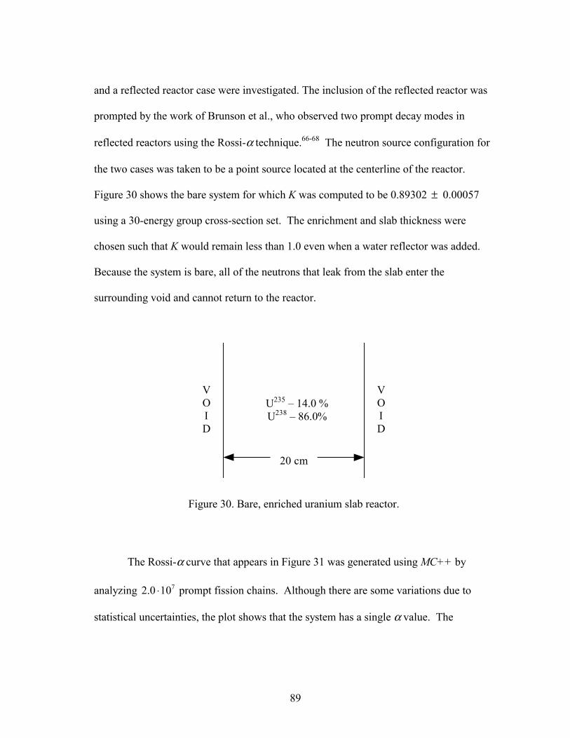
89
and a reflected reactor case were investigated. The inclusion of the reflected reactor was
prompted by the work of Brunson et al., who observed two prompt decay modes in
reflected reactors using the Rossi-α technique.66-68 The neutron source configuration for
the two cases was taken to be a point source located at the centerline of the reactor.
Figure 30 shows the bare system for which K was computed to be 0.89302 ± 0.00057
using a 30-energy group cross-section set. The enrichment and slab thickness were
chosen such that K would remain less than 1.0 even when a water reflector was added.
Because the system is bare, all of the neutrons that leak from the slab enter the
surrounding void and cannot return to the reactor.
U235 – 14.0 %U238 – 86.0%
VOID
VOID
20 cm
Figure 30. Bare, enriched uranium slab reactor.
The Rossi-α curve that appears in Figure 31 was generated using MC++ by
analyzing 72.0 10⋅ prompt fission chains. Although there are some variations due to
statistical uncertainties, the plot shows that the system has a single α value. The

90
measured α corresponds to a prompt neutron lifetime of ~30 nanoseconds which is
reasonable for a thin, fast system.
Time [sec]
0.0 2.0e-7 4.0e-7 6.0e-7 8.0e-7 1.0e-6 1.2e-6 1.4e-6 1.6e-6
Cou
nt P
roba
bilit
y [1
/sec
]
106
107
108 A = 2.26431e8α = -3.37429e6R2 = 0.9990
Figure 31. Results for a simulated Rossi-α measurement performed on a bare enriched
uranium slab.
In the reflected reactor case, some neutrons re-enter the reactor due to scattering events
occurring in a 2.5 cm thick water region on either side of the reactor (see Figure 32).
The reflector increases the prompt neutron multiplication factor to K=0.96955 ±
0.00082. Although the addition of the reflectors produces only a modest increase in K,
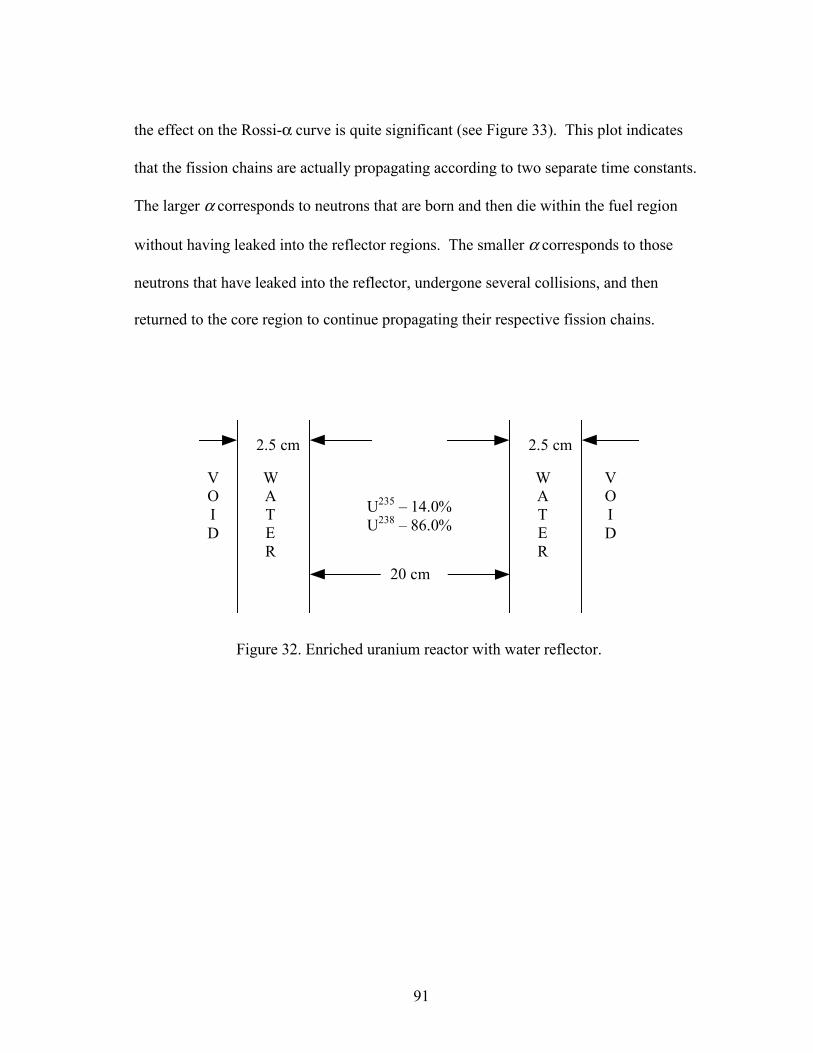
91
the effect on the Rossi-α curve is quite significant (see Figure 33). This plot indicates
that the fission chains are actually propagating according to two separate time constants.
The larger α corresponds to neutrons that are born and then die within the fuel region
without having leaked into the reflector regions. The smaller α corresponds to those
neutrons that have leaked into the reflector, undergone several collisions, and then
returned to the core region to continue propagating their respective fission chains.
WATER
WATER
VOID
VOID
U235 – 14.0%U238 – 86.0%
20 cm
2.5 cm 2.5 cm
Figure 32. Enriched uranium reactor with water reflector.

92
Time [sec]
0.0 2.0e-5 4.0e-5 6.0e-5 8.0e-5 1.0e-4 1.2e-4
Cou
nt P
roba
bilit
y [1
/sec
]
106
107
108
Figure 33. Dual decay mode Rossi-α curve in reflected slab reactor.
The data plotted in Figure 33 can be represented using two exponential terms. The
highly curved portion of the plot is shown in more detail in Figure 34. This data is
identical to the former except that the channel width has been decreased by a third. The
parameters appear in Table VIII.
1 21 2
t ty A e A eα α− −= + (IV.3)

93
TABLE VIII
Parameters for dual Rossi-α curve fit.
Exponential Term 1 Term 2 R2 A 82.1667 10⋅ 75.7001 10⋅ Dual α 6-1.1015 10⋅ 44.0012 10− ⋅
0.999563
Time [sec]
0 1e-6 2e-6 3e-6 4e-6 5e-6
Cou
nt P
roba
bilit
y [1
/sec
]
107
108
Figure 34. Expanded view of Rossi-α curvature.
I. Spatial Harmonics
Analytic solutions predict that there are an infinite number of α’s associated with
any given configuration of a multiplying system. However, when the system is very

94
near delayed critical, the fundamental mode completely dominates the solution, giving
the impression that there is only one decay mode. However, as the system becomes
increasingly subcritical, other harmonics can be resolved that have their own unique
prompt decay modes.69 For example, if the enriched uranium fuel in the slab reactor
shown in Figure 30 is exchanged for natural uranium, K drops to 0.67603 ± 0.00071.
Then, as a Rossi-α simulation with MC++ reveals in Figure 35, other modes become
observable.
Time [sec]
0.0 2.0e-7 4.0e-7 6.0e-7 8.0e-7 1.0e-6 1.2e-6 1.4e-6 1.6e-6
Cou
nt P
roba
bilit
y [1
/sec
]
101
102
103
104
105
106
107
108
Regression All Events
Figure 35. Spatial harmonics appearing in bare slab geometry.

95
A regression analysis performed on these data suggested that 3 exponential terms are
necessary to fit the data. The results appear in Table IX.
31 2
1 2 3tt ty A e A e A e αα α −− −= + + (IV.4)
TABLE IX
Parameters for regression fit of harmonic data.
Term 1 Term 2 Term 3 R2
A 2.4621x10⁷ 1.8068x10⁷ 9.7697x10⁶
αααα 5.6386x10⁷ 2.18658x10⁷ 8.2731x10⁶ 0.99999911

96
Time [sec]
0.0 2.0e-7 4.0e-7 6.0e-7 8.0e-7 1.0e-6 1.2e-6 1.4e-6 1.6e-6
Cou
nt P
roba
bilit
y [1
/sec
]
106
107
108
Figure 36. Bare slab with enriched uranium showing harmonics
Harmonics can also be resolved in systems with relatively high values of K. As
proof, a Rossi-α experiment has been simulated using the enriched uranium slab. The
results are plotted in Figure 36. The significance of this figure is the slight curvature of
the data points associated with the shortest bin widths. To verify whether the curve can
be attributed to the presence of another decay constant, the data were fit with single and
double exponential curves. The results of these fits are presented in Table X. Note that
the α’s and the amplitudes of the dual-exponential terms differ by an order of
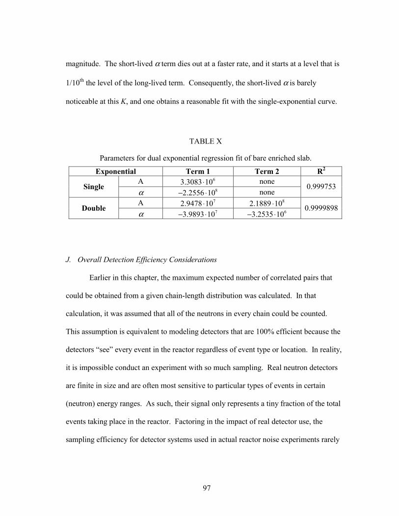
97
magnitude. The short-lived α term dies out at a faster rate, and it starts at a level that is
1/10th the level of the long-lived term. Consequently, the short-lived α is barely
noticeable at this K, and one obtains a reasonable fit with the single-exponential curve.
TABLE X
Parameters for dual exponential regression fit of bare enriched slab.
Exponential Term 1 Term 2 R2 A 63.3083 10⋅ none
Single α 82.2556 10− ⋅ none
0.999753
A 72.9478 10⋅ 82.1889 10⋅ Double
α 73.9893 10− ⋅ 63.2535 10− ⋅ 0.9999898
J. Overall Detection Efficiency Considerations
Earlier in this chapter, the maximum expected number of correlated pairs that
could be obtained from a given chain-length distribution was calculated. In that
calculation, it was assumed that all of the neutrons in every chain could be counted.
This assumption is equivalent to modeling detectors that are 100% efficient because the
detectors “see” every event in the reactor regardless of event type or location. In reality,
it is impossible conduct an experiment with so much sampling. Real neutron detectors
are finite in size and are often most sensitive to particular types of events in certain
(neutron) energy ranges. As such, their signal only represents a tiny fraction of the total
events taking place in the reactor. Factoring in the impact of real detector use, the
sampling efficiency for detector systems used in actual reactor noise experiments rarely

98
exceeds 10-4. Fortunately, this sampling efficiency is adequate for a Rossi-α
measurement when the system is operating near delayed critical. In highly subcritical
systems, however, low detector efficiencies may preclude any type of analysis within a
reasonable counting time. The Rossi-α curves in this section were computed by MC++
for the natural uranium slab reactor described in the previous section. Table XI shows
the effects on the estimate of the fastest decay mode as the detector becomes less
sensitive to certain event types. As the sensitivity decreases, the intercept of the curve
drops as the amount of data under the curve decreases (see Figure 37). This decrease
should be expected because the coefficient of the Rossi-α equation is directly
proportional to the detector efficiency. However, the difference no longer appears to be
constant when the leakage neutrons alone are available for sampling.
TABLE XI
Detector efficiency effect on fastest decay mode estimate.
Fission + Loss Loss Leakage only
A 2.447x10⁷ 1.287x10⁷ 1.291x10⁶
αααα 5.665x10⁷ 4.473x10⁷ 5.769x10⁶
R2 0.99999916 0.99999933 0.99999928

99
Time [sec]
0.0 2.0e-7 4.0e-7 6.0e-7 8.0e-7 1.0e-6 1.2e-6 1.4e-6 1.6e-6
Cou
nt P
roba
bilit
y [s
ec-1
]
101
102
103
104
105
106
107
108
Fission + LossLossLeakage only
Figure 37. Effect of population type sampled on Rossi-α data.
Figure 38 shows the predicted response of a family of leakage detectors with different
detector efficiencies. Leakage detectors (ex-core detector) were selected for simulation
since they have the least impact on the natural fission chain propagation. The only
difference between the α curves is the amount of data analyzed. The number of neutrons
entering the detector is identical, as is the simulated duration of the experiment. It is
clear that the detector with the highest efficiency, which captures every leaking neutron,
produces the smoothest curve. As the efficiency drops to a more realistic value of 410− ,

100
only one data point appears on the chart as being significantly above the background
noise. While the inefficiency of the detector does not preclude eventually obtaining a
reasonable α curve, it will take approximately 10,000 times longer to obtain the same
accuracy as it would with the detector with the perfect efficiency.
Time [sec]
0.0 2.0e-7 4.0e-7 6.0e-7 8.0e-7 1.0e-6 1.2e-6 1.4e-6 1.6e-6
Cou
nt P
roba
bilit
y [1
/sec
]
100
101
102
103
104
105
106
107
108
100%10%1%0.01%
Figure 38. Signal degradation due to decreasing detector efficiency.

101
CHAPTER V
CONCLUSIONS
A. Summary
Two codes, MC++ and Chain, have been developed that use analog Monte Carlo
techniques to simulate the spawning and propagation of fission chains. The codes
simulate the stochastic nature of fission chain formation with sufficient detail to provide
accurate chain-length distributions. The codes also provide a means for simulating a
variety of reactor configurations, source distributions, and detector types with
efficiencies. Both codes perform a variety of neutron noise analyses ranging from a
straightforward pulse-neutron die-away simulation to the time-series analysis of the
Rossi-α technique, and as such, provide a new means for simulating and re-examining
previous neutron noise experiments.
From basic theory and the use of these codes, it has been shown that neutron
noise analysis techniques are sensitive to the value of the average chain length for a
system. Depending on K, the average chain length determines the average number of
correlated pairs expected from a source neutron. While the noise signal arising from
systems with very low values of K can generally be simulated in a computer
environment, the number of source neutrons tracked must be very large to produce a
sufficient number of correlated pulses. In similar, real-world systems, it was shown that
measurements could require prohibitively long counting times depending on the source
rate. As MC++ demonstrates, the neutron source rate can only be increased until the
fission chains begin overlapping. If a detector with a low efficiency is used, the

102
probability of detecting several neutrons from the same fission chain is significantly
reduced. The loss of information must be compensated for with even longer counting
times to observe a sufficient number of correlated counts.
In addition to being a function of K, it has been shown that the chain-length
distribution is also sensitive to the type of multiplicity distribution employed in the
simulation and to the properties of the fixed neutron source that drives the problem.
The relationship, pM L= , provides an effective means for validating the average
chain length calculated with computer codes. Furthermore, it has been shown how this
value can be used to find the value of *g for a multiplying system. Finally, it has been
demonstrated that the coefficient that appears in many time-series techniques is directly
related to the chain-length distribution through the relationship,
( ) ( )
( )1
1
11 2
2 1 1L
L
L LP L
KK K L P L
ν
∞
=∞
=
−Γ � � � � =� � � �− −� � � � ⋅
�
� .
B. Future Work
MC++ can provide a means for studying topics that were beyond the scope of
this work. Specifically, MC++ could be used to study spatial-dependent reactor
kinetics. A major goal of this effort would be to fully describe the phenomena, which
produce the multiple decay modes observed in multi-region systems. Transport models
could then be developed to determine the multiple decay constants in terms of more
fundamental quantities, such as the neutron lifetimes in the various regions.

103
Chain, because of its ability to determine the asymptotic behavior of the chain-
length distributions, could also have a role in future investigations. Due to its ability to
run a much larger number of neutrons in a simulation, this code provides an excellent
means for exploring the low-probability portion of the chain-length distribution.
Currently, it is not clear whether there exists an absolute maximum chain length for a
specified K and ν , but there is a definite L which approaches infinity as 1.0K → .
What appears more likely is that the tail approaches some asymptotic value that is itself
a function of the two parameters.
Both codes would also be useful for evaluating the limitations of existing neutron
noise techniques and for developing newer ones that might be better suited to particular
applications. Although only a handful of noise analysis techniques have been
programmed into the two codes, others could be added in the future. This capability
would be most beneficial in studying the sensitivity of various noise analysis techniques
to factors like detector dead-time, efficiency, location, etc. Future work should also
include a more detailed simulation of the delayed neutron contribution.
Although the current analog Monte Carlo technique used to simulate the prompt
fission chains produces realistic results, it greatly reduces the runtime efficiency of the
two codes. One way to improve the computational efficiency might be to employ
variance reduction techniques such as those employed in other Monte Carlo packages.
While implementation of these would require only a modest coding effort, the drawback
is that these techniques must not interfere with the truly stochastic nature of the fission
chain propagation process. For any variance reduction method applied, it must be

104
determined whether its reduction of the statistical uncertainty warrants the increased
computational time and loss of fidelity in the physical model.

105
REFERENCES
1. V. L. PUTMAN, “30 September 1999 Criticality Accident, Summary to Date (991130),” INEEL/MIS-1999-1139 update, Idaho National Engineering and Environmental Laboratory (1999).
2. J. THIE, Power Reactor Noise, American Nuclear Society, La Grange Park, Illinois (1981).
3. M. M. R. WILLIAMS, Random Processes in Nuclear Reactors, Pergamon Press, New York (1974).
4. F. DE HOFFMANN, “Statistical Fluctuations in the Water Boiler and the Dispersion of Neutrons Exited Per Fission,” LA-101, Los Alamos Scientific Laboratory (1944).
5. F. DE HOFFMANN, “Intensity Fluctuations of a Neutron Chain Reactor,” LA-256, Los Alamos Scientific Laboratory (1944).
6. R. FEYNMAN, “Statistical Behavior of Neutron Chains,” LA-591, Los Alamos Scientific Laboratory (1946).
7. F. DE HOFFMANN, The Science and Engineering of Nuclear Power, Vol. II, pp. 103-109, Addison Wesley Press, Cambridge, Mass. (1949).
8. J. D. ORNDOFF, “Prompt Neutron Periods of Metal Critical Assemblies,” Nucl. Sci. Eng., 2, 450 (1957).
9. E. D. COURANT and P. R. WALLACE, “Fluctuations of the Number of Neutrons in a Pile,” Physical Review, 72, 1038 (1947).
10. C. E. COHN, “A Simplified Theory of Pile Noise,” Nucl. Sci. Eng., 7, 472 (1960).
11. W. MATTHES, “Statistical Fluctuations and Their Correlation in Reactor Neutron Distributions,” Nukleonik, 4, 213 (1962).
12. G. I. BELL, “Probability Distribution of Neutrons and Precursors in a Multiplying Assembly,” Ann. of Phys., 21, 243 (1963).
13. D. R. HARRIS, “Neutron Fluctuations in a Reactor of Finite Size,” Nucl. Sci. Eng., 21, 369 (1965).
14. H. BORGWALDT and D. STEGMANN, “A Common Theory for Neutronic Noise Analysis Experiments in Nuclear Reactors,” Nukleonik, 7, 313 (1965).

106
15. R. A. RYDIN, J. A. BURKE, W. E. MOORE, and K. W. SEEMANN, “Noise and Transient Kinetics Experiments and Calculations for Loosely Coupled Cores,” Nucl. Sci. Eng., 46, 179 (1971).
16. G. SPRIGGS, “The Reactor Noise Threshold,” Nucl. Sci. Eng., 116, 67 (1994).
17. J. MIHALCZO, V. PARE, and E. BLAKEMAN, “Fission Chain Length Effects on Californium-Source-Driven Subcriticality Measurements,” International Conference on Advances in Mathematics, Computation, and Reactor Physics, American Nuclear Society, Pittsburgh, Pennsylvania, April 28 (1991).
18. J. MIHALCZO, E. BLAKEMAN, V. PARE, T. VALENTINE, and D. AUSLANDER, “Subcriticality of Two Uranyl Nitrate Flat Cylindrical Tanks Spaced in Air by 252Cf-Source-Driven Noise Analysis,” Nucl. Tech., 103, 346 (1993).
19. R. FEYNMAN, F. DE HOFFMANN, and R. SERBER, “Dispersion of the Neutron Emission in U-235 Fission,” J. Nucl. Energy, 3, 64 (1956).
20. R. B. LEACHMAN, “Emission of Prompt Neutrons from Fission,” Physical Review, 101, 1005 (1956).
21. B. C. DIVEN, H. C. MARTIN, R. F. TASCHEK, and J. TERRELL, “Multiplicities of Fission Neutrons,” Physical Review, 101, 1012 (1956).
22. J. TERRELL, “Distributions of Fission Neutron Numbers,” Physical Review, 108, 783 (1957).
23. J. TERRELL, “Fission Neutron Spectra and Nuclear Temperatures,” Physical Review, 113, 2, 527 (1958).
24. J. TERRELL, “Neutron Yields from Individual Fission Fragments,” Physical Review, 127, 880 (1962).
25. N. E. HOLDEN and M. S. ZUCKER, “Prompt Neutron Multiplicities for the Transplutonium Nuclides,” BNL-NCS-36379, International Conference on Nuclear Data for Basic and Applied Science, Santa Fe, NM (1985).
26. J. W. BOLDMAN and M. G. HINES, “Prompt Neutron Emission Probabilities Following Spontaneous and Thermal Neutron Fission,” Nucl. Sci. Eng., 91, 114 (1985).
27. J. FREHAUT, “Neutron Multiplicity Distribution in Fast Neutron-Induced Fission,” IAEA Consultants Meeting on Physics of Neutron Emission in Fission, May 1988, Mito, Japan (1989).

107
28. D. HAWKINS and S. ULAM, “Theory of Multiplicative Process, I,” LA-171, Los Alamos Scientific Laboratory (1944).
29. G. E. HANSEN, “Assembly of Fissionable Material in the Presence of a Weak Neutron Source,” Nucl. Sci. Eng., 8, 709 (1960).
30. H. HURWITZ, JR., “Kinetics of Low Source Reactor Startups. Part I,” Nucl. Sci. Eng., 15, 166 (1963).
31. H. HURWITZ, JR., “Kinetics of Low Source Reactor Startups. Part II,” Nucl. Sci. Eng., 15, 166 (1963).
32. G. I. BELL, “On the Stochastic Theory of Neutron Transport,” Nucl. Sci. Eng., 21, 369 (1965).
33. G. A. CAMPBELL, V. CHAN, and J. D. LEWINS, “An Exact Special Case Solution of the Neutron Stochastic Equations at Low Power,” Ann. Nucl. Energy, 8, 1 (1981).
34. F. C. DIFILIPPO, “Stochastic Processes in a Subcritical Nuclear Reactor in the Presence of a Fission Source,” Nucl. Sci. Eng., 90, 13 (1985).
35. J. D. LEWINS and G. T. PARKS, “An Exact Transient Stochastic Solution for Low-Power Neutron Multiplication,” Ann. Nucl. Energy, 12, 65 (1985).
36. L. RUBY and T. L. MCSWINE, “Approximate Solution to the Kolmogorov Equation for a Fission Chain-Reacting System,” Nucl. Sci. Eng., 94, 271 (1986).
37. J. MUNOZ-COBO, R. B. PEREZ, and G. VERDU, “Stochastic Neutron Transport Theory: Neutron Counting Statistics in Nuclear Assemblies,” Nucl. Sci. Eng., 95, 83 (1987).
38. R. SANCHEZ, “An Analysis of the Stochasticity of the Transport Equation,” Trans. Theory Stat. Phys., 26, 469 (1997).
39. I. PAZIT, and Y. YAMANE, “Theory of Neutron Fluctuations in Source-Driven Subcritical Systems,” Nucl. Inst. Meth. in Phys. Res. Sect. A, 403, 431 (1998).
40. J. BRIESMEISTER ed., “MCNP-A General Monte Carlo N-Particle Transport Code, Version 4B,” LA-12625-M, Version 4B Los Alamos National Laboratory (1997).
41. T. E. HARRIS, The Theory of Branching Processes, Dover Publications, Inc., New York (1989).
42. P. GUTTORP, Statistical Inference for Branching Processes, John Wiley & Sons, Inc., New York (1991).

108
43. T. F. WIMMETT, R. H. WHITE, W. R. STRATTON, and D. P. WOOD, “Godiva II—An Unmoderated Pulse-Irradiation Reactor,” Nucl. Sci. Eng., 8, 691 (1960).
44. J. DUDERSTADT and L. HAMILTON, Nuclear Reactor Analysis, John Wiley & Sons, New York (1976).
45. G. SPRIGGS, “Two Rossi-α Techniques for Measuring the Effective Delayed Neutron Fraction,” Nucl. Sci. Eng., 113, 161 (1993).
46. G. SPRIGGS, S. OKAJIMA, T. SAKURAI, and R. B. BUSCH, “The Equivalent Fundamental-Mode Source,” LA-UR-97-1, Los Alamos National Laboratory (1997).
47. R. E. UHRIG, Random Noise Techniques in Nuclear Reactor Systems, Ronald Press Co., New York (1970).
48. C. P. BAKER, “Time Scale Measurements by the Rossi Method,” LA-617, Los Alamos Scientific Laboratory (1947).
49. D. H. BRYCE, “Some Comments on the Rossi-α Experiment,” Nukleonik, 7, 428 (1965).
50. D. BABALA, “On the Theory of Rossi-Alpha Experiment in Reactor Noise Studies,” Nucl. Sci. Eng., 26, 418 (1966).
51. D. BABALA, “Point-Reactor Theory of Rossi-Alpha Experiment,” Nucl. Sci. Eng., 28, 237 (1967).
52. D. BABALA, “Interval Distributions in Neutron Counting Statistics,” Nucl. Sci. Eng., 28, 243 (1967).
53. T. IIJIMA, “A Remark on the Rossi-α Experiment,” Nukleonik, 10, 93 (1967).
54. N. PACILIO, “Reactor Noise Analysis in the Time Domain,” USAEC Critical Review Series, TID-24512 (1969).
55. T. MISAWA, H. UNESAKI, S. SHIROYA, and Y. YAMANE, “Study on Reactivity Measurement by the Feynman-α Method,” PHYSOR 96: International Conference on the Physics of Reactors, 16-20 Sep., Mito, Japan, (1996).
56. G. E. HANSEN, “The Rossi Alpha Method,” Workshop on Subcritical Reactivity Measurements, Aug. 1985, Albuquerque, N.M., 148, CONF-8508105 (1985).
57. S. OKAJIMA, M. NARITA, and K. KOBAYASHI, “Simple Determination of Low Power on Reflected Reactors Using the Feynman-α Experiment,” Ann. Nucl. Energy, 14, 673 (1987).

109
58. I. PAZSIT and Y. YAMANE, “The Variance-to-Mean Ratio in Subcritical Systems Driven by a Spallation Source,” Ann. Nucl. Energy, 25, 667 (1998).
59. S. R. LEE, “MC++: A Brief Overview of a Work in Progress,” LA-MEMO XTM:96-219(U), Los Alamos National Laboratory (1996).
60. S. R. LEE, J. C. CUMMINGS, and S. D. NOLEN, “Preliminary MC++ Timing and Physics Results,” X-Division Research Notes, XTM-RN(U)96-005, Los Alamos National Laboratory (1996).
61. S. R. LEE, J. C. CUMMINGS, and S. D. NOLEN, “MC++: Parallel, Portable, Monte Carlo Neutron Transport in C++,” 8th SIAM Conference on Parallel Processing for Scientific Computing, March 14 Minneapolis, MN (1997).
62. J. MARSHALL, S. CLANCY and L. ANKENY, “Tecolote: An Object-Oriented Framework for Physics Development,” European Conference for Object-Oriented Programming, Brussels, Belgium, LA-UR-98-2999, (1998).
63. J. REYNDERS, T. WILLIAMS, J. CUMMINGS, and S. HANEY, “POOMA: A Framework for Scientific Simulations on Parallel Architectures,” in G. WILSON and P. LU, eds., Parallel Programming using C++, MIT Press, Cambridge, MA, 553 (1996).
64. J. REYNDERS, “POOMA Homepage,” online: http://www.acl.lanl.gov/pooma, accessed: March 2000.
65. A. SNOOD, R. A. FORSTER, and D. K. PARSONS, “Analytical Benchmark Test Set for Criticality Code Verification,” LA-13511, Los Alamos National Laboratory (1999).
66. G. S. BRUNSON, R. N. CURRAN, J. M. GASIDLO and R. J. HUBER, “Neutron Die-Away Phenomena,” Trans. Amer. Nucl. Soci., 6, 56 (1963).
67. G. S. BRUNSON, R. N. CURRAN, J. M. GASIDLO and R. J. HUBER, “A Survey of Prompt-Neutron Lifetimes in Fast Critical Systems,” Argonne National Laboratory, ANL-6681 (1963).
68. G. S. BRUNSON and R. J. HUBER, “Two-Region Analysis of Pulsing Data in Fast Critical Systems,” Nucl. Instr. Methods, 128, 379 (1975).
69. T. IIJIMA, T. SUGI, H. EZURE, and M. KASAI, “Space-Dependent Effects in Rossi-Alpha Experiments,” Nucl. Sci. Eng., 33, 344 (1968).

110

111
VITA
Steven Douglas Nolen was born in Lubbock, Texas, in 1971. He earned a B.S. in
Nuclear Engineering at Texas A&M University in 1994. In December of 1997, he
earned a M.S. in Nuclear Engineering. During this time, he began his association with
Los Alamos National Laboratory’s X-Division which has culminated in the work
presented herein. He is currently a post-doctoral researcher at the laboratory. His
mailing address in 1990 40th St. Los Alamos, New Mexico 87544.

This report has been reproduced directly from thebest available copy. It is available electronically onthe Web (http://www.doe.gov/bridge).
Copies are available for sale to U.S. Department ofEnergy employees and contractors from—
Office of Scientific and Technical InformationP.O. Box 62Oak Ridge, TN 37831(423) 576-8401
Copies are available for sale to the public from—
National Technical Information ServiceU.S. Department of Commerce5285 Port Royal RoadSpringfield, VA 22616(800) 553-6847

LosN A T I O N A L L A B O R A T O R Y
AlamosLos Alamos, New Mexico 87545