Embed Size (px)
Citation preview

THE IMPACT OF TRAINING ON
PRODUCTIVITY AND WAGES:EVIDENCE FROM BRITISH PANEL DATA
Lorraine DeardenHoward Reed
John Van Reenen
THE INSTITUTE FOR FISCAL STUDIES
WP05/16

1
The Impact of Training on Productivity and Wages: Evidence from British Panel Data* LORRAINE DEARDEN,† HOWARD REED‡ AND JOHN VAN REENEN§ † Institute for Fiscal Studies (e-mail: [email protected]) ‡ Institute for Public Policy Research (e-mail: [email protected]) § Centre for Economic Performance, London School of Economics and CEPR; Houghton Street, London, WC1E 2AE (e-mail: [email protected]) Abstract It is standard in the literature on training to use wages as a sufficient statistic for productivity. This paper examines the effects of work-related training on direct measures of productivity. Using a new panel of British industries 1983-1996 and a variety of estimation techniques we find that work-related training is associated with significantly higher productivity. A one percentage point increase in training is associated with an increase in value added per hour of about 0.6% and an increase in hourly wages of about 0.3%. We also show evidence using individual level datasets that is suggestive of training externalities. JEL classification numbers J31; C23; D24 Keywords Productivity, training, wages, panel data
* Financial support from the Economic and Social Research Council and the Leverhulme Trust is gratefully acknowledged. We would like to thank Fernando Galindo-Ruedo, Amanda Gosling, Richard Layard, Lisa Lynch, Stephen Machin, Steve McIntosh, Alan Manning, Steve Pischke, two anonymous referees and participants in many seminars for helpful comments. We are grateful to the Office for National Statistics for supplying the Census of Production data and to the OECD for supplying the ISDB data. We would like to thank Martin Conyon for supplying the firm-level training data and Jonathan Haskel for providing us with some of the industry price indices used in the paper. Material from the Labour Force Survey is Crown Copyright, has been made available by the Office for National Statistics through the ESRC Data Archive and has been used by permission. Neither the ONS nor the Data Archive bears any responsibility for the analysis or interpretation of the data reported here. An earlier version of this paper (with a longer data description) has appeared as ‘Who gains when workers train’, Working Paper No. 00/04, Institute for Fiscal Studies.

2
I. Introduction
It is a widely-held view that Britain needs to increase work-related training to
improve long-term economic performance and address the ‘skills gap’.1
Despite the policy interest and the huge economics literature on human
capital, there are hardly any papers that examine the impact of work-related
training on direct measures of productivity. The primary contribution of our
paper is to provide such evidence for the first time in the UK and for the first
time anywhere over a long period (we have 14 years of data). Analysis of the
impact of training on productivity has focused almost entirely on estimating the
impact of training on wages. Most studies looking at the private return to work-
related training find that training results in workers receiving higher real
wages.2
Although these studies are informative, they only tell half the story as
they ignore the impact on the employer’s productivity. The relationship
between wage increases and productivity gains can vary according to the
structure of the labour and product markets and according to who actually
pays the costs of training. In the simplest neoclassical view of the labour
market where the market is perfectly competitive, wages will be equal to the
value of marginal product. Thus the wage can be taken as a direct measure of
productivity. This simple relationship can break down for many reasons. For
example, in Becker’s model of specific human capital, the employer will pay
for training, so there should be no effect of completed training spells on
observed wages even though there may be a large impact on productivity.3
1 See Green and Steedman (1997) or National Skills Task Force (1998). In the December 2003 Pre-Budget Report, the British Chancellor justified the extension of the Employer Training Pilots in order to help improve the skills gap and UK productivity. (http://www.hm-treasury.gov.uk/media//2E3BD/03_Meeting%20the%20Pro_EF.pdf) 2 See Greenhalgh and Stewart (1987), Booth (1991, 1993) or Blundell et al. (1996) for UK evidence. US studies using panel data include Lillard and Tan (1992), Lynch (1992), Blanchflower and Lynch (1992) and Bartel and Sicherman (1999). Winkelmann (1994) uses German data and Bartel (1995) looks within a large US manufacturing company. 3 There are many other reasons for a wedge between productivity and wage in a competitive labour market. First, employees may receive non-pecuniary benefits from training. Second, workers may implicitly pay the costs of a training scheme in the form of lower wages whilst being trained, which then rise after training is completed – so we might see a greater increase in observed wages than in productivity. Third, employees’ wages could be lower during training because they are not contributing to firm productivity whilst actually being trained. Fourth, there may be deferred compensation packages where the employee’s remuneration is ‘backloaded’ towards later post-training years as a means of ensuring loyalty and/or effort early in the employee’s tenure (e.g. Lazear, 1979).

3
If the labour market is characterised by imperfect competition then the
strict link between wages and productivity is usually broken. Employees can
find themselves being paid less (or more) than their marginal revenue product.
Nevertheless, it is still the case that conditional on a given degree of rent-
sharing or monopsony power; increases in wages have to be paid out of
productivity gains. Therefore we can assert the general principle that these
real wage increases should provide a lower bound on the likely size of
productivity increases. In practice, the productivity gains are likely to be higher
than this. For instance, in a labour market with frictions and some wage
compression (e.g. from a binding minimum wage), there will be productivity
gains even from general training that are not passed on to the employee in
terms of wages but are only reflected in direct measures of productivity.4
Similar results can be found in some bargaining models (e.g. Booth et al.,
1999).
There exist a small number of empirical papers that relate firm
productivity to a measure of training.5 Although a positive correlation is
generally found, it is very difficult to interpret because the training measures
are only measured at a single point of time and could be picking up many
unobservable firm-specific factors correlated with both training and
productivity. Black and Lynch (2001) used an establishment training survey at
two points of time. In the cross section, they identified some effects of the type
of training on productivity, but they found no significant association when they
controlled for plant-specific effects. Ichniowski et al. (1997) investigated what
factors influence productivity in a panel of US steel finishing mills. After
controlling for fixed effects, they found a role for training only in combination
with a large variety of complementary human resource practices. Carriou and
Jeger (1997), Ballot et al. (1998) and Delame and Kramarz (1997) used
French firm-level panel data to look at the effects of training on value added
and found positive and significant effects. Although these studies are broadly
4 See Acemoglu and Pischke (1999, 2003). 5 Black and Lynch (1996), Bartel (1994), Barrett and O’Connell (2001), de Koning (1994), Boon and van der Eijken (1997) and Ballot and Taymaz (1998) have objective productivity measures. Bartel (1995), Holzer (1990), Barron et al. (1989) and Krueger and Rouse (1998) use subjective measures of productivity. Holzer et al. (1993) do find effects of changes in productivity on changes in one measure of quality – the scrap rate.

4
consistent with our own, they do not fully exploit the potential of their panel
data by allowing training to be a choice variable.6
Our contribution in this paper is to advance the literature in at least
three ways. Black and Lynch (2001) emphasise the problems of trying to
identify the effects of training in a short panel (they have only two separate
training observations). Although unobserved heterogeneity can be controlled
for through fixed effects with only two periods, attenuation biases due to
measurement error are exacerbated. To address this, we build a panel that
contains up to 14 consecutive years of training data. Second, we explicitly
allow training to be a choice variable by using General Method of Moments
(GMM) estimators developed to deal with endogenous variables in production
functions. Third, we combine estimation of the productivity effects of training
with estimation of the wage effects of training. Although comparisons between
the production function and the wage equation are becoming more common
for other worker characteristics such as gender and human capital, this is the
first time the strategy has been used for training.7 In principle, this allows us to
examine whether trained workers are paid the value of their marginal product.
We conduct our main analysis of the effects of training at the industry
level (although we have also performed estimation at the firm and individual
level for comparative purposes). There is simply no alternative to this strategy
if one wishes to use long time series of training and productivity information.
The only publicly available firm-level panel data in the UK is a sample of about
119 firms in the late 1990s with only very basic training information (a concise
investigation of this is presented in Appendix B). Aggregation has pros and
cons that are discussed in the paper. On the positive side, if there are
important spillovers to training within an industry (e.g. through a faster rate of
innovation) then a firm-level analysis will potentially miss out these linkages
and underestimate the return to human capital.8 On the negative side, there
6 See Greenhalgh (2002) for a much more extensive review of the French and UK literature in this area. 7 Hellerstein et al. (1999), Hellerstein and Neumark (1999), Hægeland and Klette (1999) and Jones (2001) examine the differential impact of human capital and gender on wages and productivity. A recent study that utilises our methodology and looks at this question using a panel of French and Swedish firms is Ballot et al. (2002). They find that both French and Swedish firms appropriate a high proportion of the returns to training (82% and 67% respectively). 8 For example, O’Mahony (1998) finds that the coefficient on labour skills in a production function is more than twice that assumed by traditional growth accounting from relative wages. Other recent papers that have looked at the impact of human capital on directly measured productivity include Moretti (2004) on US data and Haskel et al. (2003) on UK data.

5
may be aggregation biases at the sectoral level that could lead to negative or
positive biases on the training coefficient. We follow Grunfeld and Griliches
(1960) in arguing that the pros of aggregation probably outweigh the cons.
The format of the paper is as follows. Section II describes the simple
economic models of productivity and wages that we will estimate and Section
III details the econometric strategy. The data are described in Section IV and
the results are presented in Section V. Section VI offers some concluding
comments. Appendix A contains more information on the data and some
additional experiments. Our main result is that we find a statistically and
economically significant effect of training on industrial productivity. A 1
percentage point increase in training is associated with about a 0.6% increase
in productivity and a 0.3% increase in hourly wages. The productivity effect of
training is twice as large as the wage effect, implying that existing studies
have underestimated the benefits of training by focusing on wages.
II. A model of training and productivity
To see our approach, assume that we can characterise a representative plant
in an industry by a Cobb–Douglas production function written in value added
form9 βα KALQ = (1)
where Q is value added, L is effective labour input allowing for quality and
quantity dimensions, K is capital and A is a Hicks neutral efficiency parameter.
We consider that trained workers are more productive than untrained
workers, so that effective labour input can be written as TU NNL γ+= (2)
where NU is the number of untrained workers, NT is the number of trained
workers and γ is a parameter which, if trained workers are more productive
than non-trained workers, will be greater than unity. The total number of
workers, N, is equal to the sum of trained and untrained workers. Substituting
equation (2) into equation (1) gives
[1 ( 1) ]Q A TRAIN N Kα α βγ= + − (3)
9 This should be viewed as a first-order approximation to a more complicated functional form. It is straightforward to generalise this to more complex functional forms such as translog and some experiments are included in the empirical results.
6
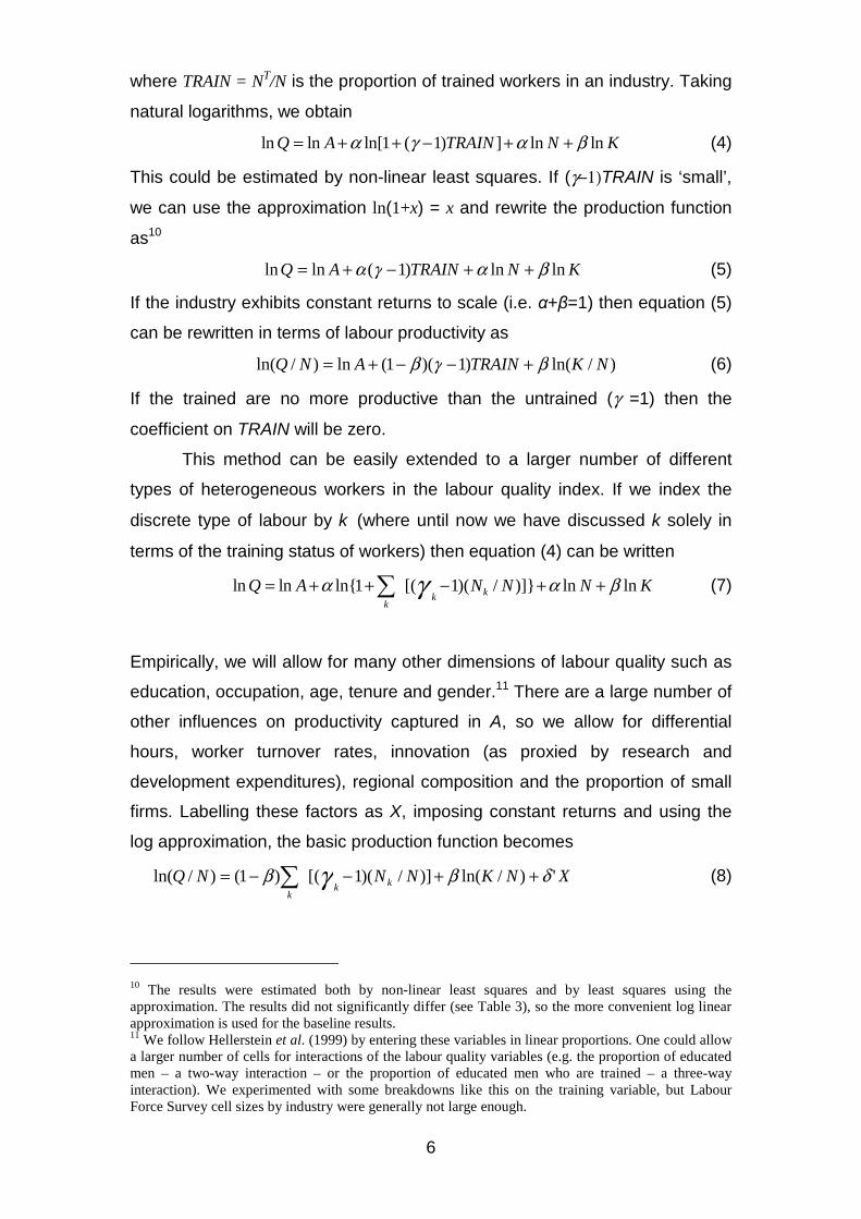
where TRAIN = NT/N is the proportion of trained workers in an industry. Taking
natural logarithms, we obtain
ln ln ln[1 ( 1) ] ln lnQ A TRAIN N Kα γ α β= + + − + + (4)
This could be estimated by non-linear least squares. If (γ−1)TRAIN is ‘small’,
we can use the approximation ln(1+x) = x and rewrite the production function
as10
KNTRAINAQ lnln)1(lnln βαγα ++−+= (5)
If the industry exhibits constant returns to scale (i.e. α+β=1) then equation (5)
can be rewritten in terms of labour productivity as
)/ln()1)(1(ln)/ln( NKTRAINANQ βγβ +−−+= (6)
If the trained are no more productive than the untrained (γ =1) then the
coefficient on TRAIN will be zero.
This method can be easily extended to a larger number of different
types of heterogeneous workers in the labour quality index. If we index the
discrete type of labour by k (where until now we have discussed k solely in
terms of the training status of workers) then equation (4) can be written
ln ln ln{1 [( 1)( / )]} ln lnkkk
Q A N N N Kα α βγ= + + − + +∑ (7)
Empirically, we will allow for many other dimensions of labour quality such as
education, occupation, age, tenure and gender.11 There are a large number of
other influences on productivity captured in A, so we allow for differential
hours, worker turnover rates, innovation (as proxied by research and
development expenditures), regional composition and the proportion of small
firms. Labelling these factors as X, imposing constant returns and using the
log approximation, the basic production function becomes
XNKNNNQ kkk
')/ln()]/)(1[()1()/ln( δββ γ ++−−= ∑ (8)
10 The results were estimated both by non-linear least squares and by least squares using the approximation. The results did not significantly differ (see Table 3), so the more convenient log linear approximation is used for the baseline results. 11 We follow Hellerstein et al. (1999) by entering these variables in linear proportions. One could allow a larger number of cells for interactions of the labour quality variables (e.g. the proportion of educated men – a two-way interaction – or the proportion of educated men who are trained – a three-way interaction). We experimented with some breakdowns like this on the training variable, but Labour Force Survey cell sizes by industry were generally not large enough.

7
The wage equation that we estimate parallels the productivity equation in (8).
We view the wage equation as more of a descriptive regression than the
structurally derived production function. Under competitive spot markets for
labour, relative wages should equal the relative marginal productivities of
workers of different types. This is because if the relative productivity of trained
workers, γ, exceeded the relative wages of trained workers then employers
would only employ trained workers (Hellerstein et al., 1999).
Consider the wage bill, W, for the representative plant in an industry.
Again, take the simplest model where there are only two types of workers:
trained workers paid average wage wT and untrained workers paid average
wage wNT. Relative wages are λ = wT /wNT. By definition,
W = wNT(N – NT) + λ wNTNT = wNT[N+(λ–1) NT] (9)
In logarithms, the average wage (w) is
ln ln( / ) ln[1 ( 1) ]w W N a TRAINλ= = + + − (10)
where a = ln(wNT).
Clearly, estimation of equation (10) can be used to recover the relative
wage mark-up associated with training, λ, and then compared to the relative
productivity effect of training, γ. Parallel to the productivity equation, we will
allow for multiple types of labour quality, capital and other factors to influence
wages. The empirical wage equation to be estimated is therefore12:
XKNNaw wwkk
k
'ln)]/)(1[(ln δβλ ++−+= ∑ (11)
III. Econometric modelling strategy
The basic equation we wish to estimate can be written in simplified form as
ititit uxy += θ (12)
where y is Q/N and x is a vector of (suspected endogenous) variables
including training. Subscript i indicates the representative firm in an industry, t
12 One could argue that firm variables such as capital intensity and R&D should be excluded from the wage equation under competitive labour markets. However, these variables are typically quite informative in wage equations, either because they are picking up some measure of unobserved labour quality (Hellerstein and Neumark, 1999) or because of departures from perfect competition. In either case, omitting such variables is likely to cause bias on the training variable and our baseline specifications will include them.

8
is time and θ is the parameter of interest. Assume that the stochastic error
term, uit, takes the form
ititit
ittiitu
υρωωωτη
+=++=
−1
(13)
The tτ represent macroeconomic shocks captured by a series of time
dummies, iη is an individual effect and itυ is a serially uncorrelated mean
zero error term. The other element of the error term, itω , is allowed to have an
AR(1) component (with coefficient ρ ), which could be due to measurement
error or slowly evolving technological change. Substituting (13) into (12) gives
us the dynamic equation
ittiitititit xxyy υτηπππ +++++= −−**
13211 (14)
The common factor restriction (COMFAC) is 321 πππ −= . Note that
t*τ = 1−− tt ρττ and *
iη = (1– ρ )ηi.
In our main results section, we present several econometric estimates
of production functions (random effects, within groups and GMM). The most
rigorous approach follows that recommended by Blundell and Bond (2000),
which uses a ‘system GMM’ approach to estimate equation (14) and then
imposes the COMFAC restrictions by minimum distance. We now turn to
describing the GMM approach in more detail.
How should equation (14) be estimated? If training is strictly exogenous
and there are no dynamics (i.e. ρ = 0) then the only problem with OLS
estimation of (12) is the presence of the individual effects, iη . If these
individual effects are uncorrelated with xit then the random-effects estimator is
unbiased and efficient. If the individual effects are correlated with xit but
remain strictly exogenous then although the random-effects estimator is
biased, the within-groups estimator will be unbiased.
If we allow training to be endogenous (i.e. allowing training decisions to
react to shocks to current productivity), we will require instrumental variables.
In the absence of any obvious natural experiments, we consider moment
conditions that will enable us to construct a GMM estimator for equation (14).
A common method would be to take first differences of (14) to sweep out the
fixed effects:

9
*1 1 2 3 1 tit it it it ity y x xπ π π τ υ− −∆ = ∆ + ∆ + ∆ + ∆ + ∆ (15)
Since itυ is serially uncorrelated, the moment condition
0)( 2 =∆− ititxE υ (16)
ensures that instruments dated t–2 and earlier13 are valid and can be used to
construct a GMM estimator for equation (14) in first differences (Arellano and
Bond, 1991). A problem with this estimator is that variables with a high degree
of persistence over time (such as capital) will have very low correlation
between their first difference ( itx∆ ) and the lagged levels being used as
instruments (e.g. 2−itx ). This problem of weak instruments can lead to
substantial bias in finite samples.
Blundell and Bond (1998) point out that under a restriction on the initial
conditions, another set of moment conditions are available:14
0))(( 1 =+∆ − itiitxE υη (17)
This implies that lags of the first differences of the endogenous variables can
be used to instrument the levels equation (14) directly. The econometric
strategy is then to combine the instruments implied by the moment conditions
(16) and (17). We stack the equations in differences and levels, i.e. (14) and
(15). We can obtain consistent estimates of the coefficients and use these to
recover the underlying structural parameters in (12).
The estimation strategy assumes the absence of serial correlation in
the levels error terms ( itυ ).15 We report serial correlation tests in addition to
the Sargan-Hansen test of the over-identifying restrictions in all the GMM
results below.16
13 Additional instruments dated t–3, t–4, etc. become available as the panel progresses through time. 14 The restrictions are that the initial change in productivity is uncorrelated with the fixed effect
0)( 2 =∆ iiyE η and that initial changes in the endogenous variables are also uncorrelated with the
fixed effect 0)( 2 =∆ iixE η . 15 If the process is MA(1) instead of MA(0) then the moment conditions in (16) and (17) no longer
hold. Nevertheless 0)( 3 =∆− ititxE υ and 0))(( 2 =+∆ − itiitxE υη remain valid, so earlier-dated
lags could still be used as instruments. This is the situation empirically with the wage equations. 16 These are based on the first-differenced residuals, so we expect significant first-order serial correlation but require zero second-order serial correlation for the instruments to be valid. If there is significant second-order correlation, we need to drop the instruments back a further time period (this happens to be the case for the wage equation in the results below).

10
This GMM ‘system’ estimator has been found to perform well in Monte
Carlo simulations (Blundell and Bond, 1998) and in the context of the
estimation of production functions (Blundell and Bond, 2000). The procedure
should also be a way of controlling for transitory measurement error (the fixed
effects control for permanent measurement error). Random measurement
error has been found to be a problem in the returns to human capital
literature, typically generating attenuation bias (see Card, 1999).
In order to assess the importance of biases associated with fixed
effects and endogeneity, we will estimate random-effects, within-groups and
GMM estimates in the results section.
Finally, consider two more issues which are harder to deal with:
aggregation and training stocks vs. training flows. Estimation at the three-digit
industry level has advantages but also disadvantages relative to micro-level
estimation. The production function in equation (1) at the firm level describes
the private impact of training on productivity. However, many authors,
especially in the endogenous growth literature (e.g. Aghion and Howitt, 1998),
have argued that there will be externalities to human capital acquisition. For
example, workers with higher human capital are more likely to generate new
ideas, which may spill over to other firms.17 If spillovers are industry specific,
this implies that there should be additional terms added to equation (5)
representing training in other firms (e.g. the mean number of trained workers
in the industry). In this case, the coefficient on training in an industry-level
production function should exceed that in a firm-level production function.18
Second, grouping by industry may smooth over some of the measurement
error in the micro data and therefore reduce attenuation bias.
On the negative side, there may be aggregation biases in industry-level
data. A priori it is not possible to unambiguously sign these biases. We expect
that the fixed effects will control for some of the problem. For example, we are
taking logs of means and not the means of logs in aggregating equation (4),
but so long as the higher-order moments of the distributions are constant over
time in an industry then they will be captured by a fixed effect.19 If the
17 Although there are many papers that examine externalities of R&D (e.g. see the survey by Griliches, 1992) and a few that look at human capital (Acemoglu and Angrist, 2000; Moretti, 2004), there are none that focus on training spillovers. 18 For the same argument in the R&D context, see Griliches (1992). 19 If they evolve at the same rate across industries, they will be picked up by the time dummies.

11
coefficients are not constant across firms in equation (4), but are actually
random, this will also generate higher-order terms at the industry level. In the
empirical results, we experiment with including higher-order moments and
allowing the coefficients to vary across cross-sectional units.
Turning to the problem of training stocks and flows, note that the model
in equation (1) assumes that we know the stocks of trained workers in an
industry. What we actually have in the data is an estimate of the proportion of
workers in an industry who received training in a given four-week period (the
training flow). Since individuals are sampled randomly over time in the Labour
Force Survey (LFS), this should be an unbiased estimate of the proportion of
people in training in a given industry in a given year.20 As an alternative to
using the flow, we calculate a stock of training in an analogous way to using
investment flows to calculate a capital stock through the perpetual inventory
method (the main form of depreciation is the turnover rate). This is described
in Appendix A.
IV. Data description
The database we construct combines several sources (see Appendix A for full
details). The critical individual-level source is the individual-level UK Labour
Force Survey, which contained about 60,000 households per year. Most
importantly, the LFS has a consistent training measure since 1984 as well as
detailed information on skills, demographics, hours worked, tenure and
wages. We work with this information aggregated by broadly three-digit
industries. The LFS only started asking questions on wages at two points of
time in 1997 (and at one point of time in 1992 when the panel was set up). We
present some individual-level panel wage regressions at the end of Section V
for comparison.
The second major dataset we use is the Annual Census of Production
(ACOP). This gives production statistics on capital, wages, labour and output,
for industries in the production sector (manufacturing, mining and utilities). For
the services industries, we drew on the OECD’s ISDB data.
20 If there are many multiple training spells in the month, we will underestimate the proportion of employees who are being trained. If Spring (the LFS quarter we use) is a particularly heavy training season then we will overestimate the proportion being trained in a year. These biases are likely to be small and offsetting.

12
There was a change in SIC classification in 1992 which forced us to
aggregate some of the industries and prevented us from using some of the
industries after the change. Additionally, we insisted on having at least 25
individuals in each cell in each year. After matching the aggregated individual
data from LFS, we were left with 94 industry groupings over (a maximum of)
14 years.
The main LFS training question was ‘over the 4 weeks ending Sunday
… have you taken part in any education or training connected with your job, or
a job that you might be able to do in the future?’.21 The average proportions of
employees undertaking training grew steadily from about 8% in 1984 to 14%
in 1990 where it stabilised for the next six years. Most of this growth was
upgrading within industry rather than between industries.22
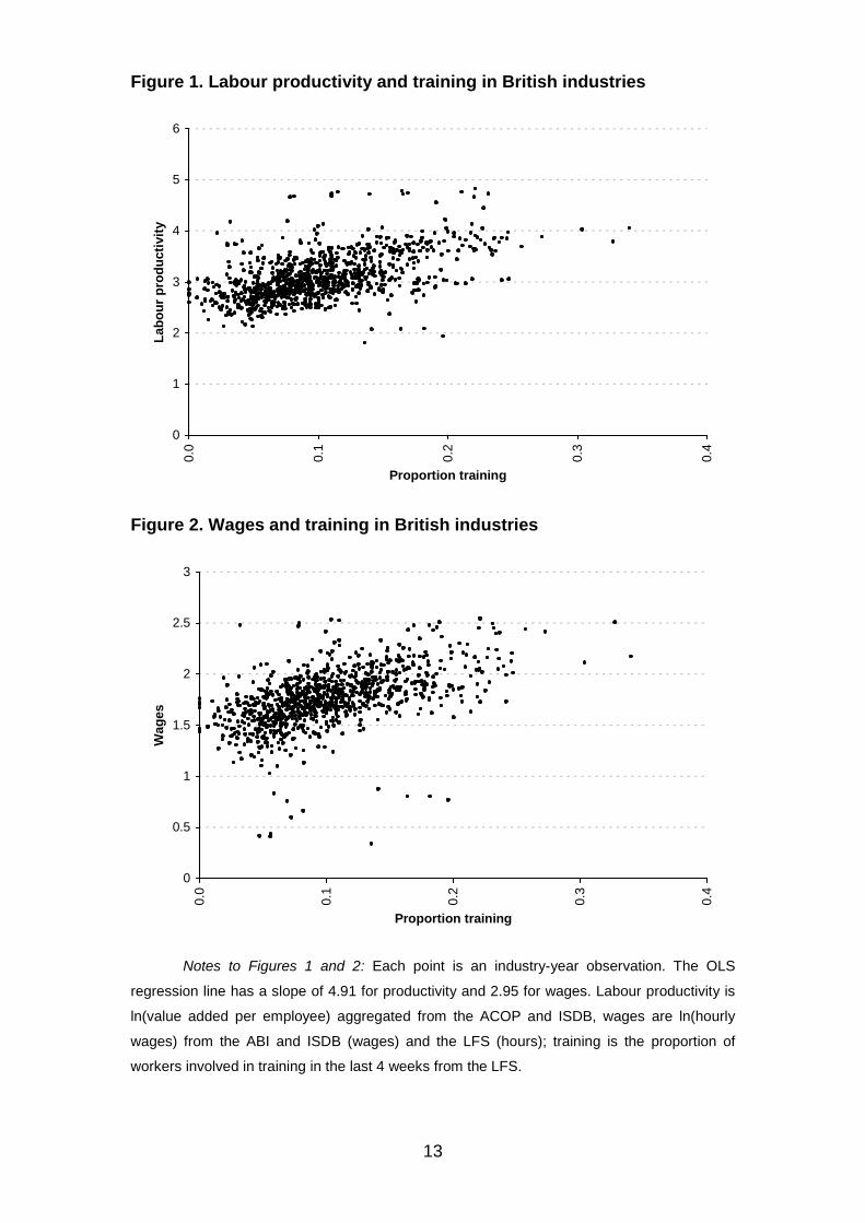
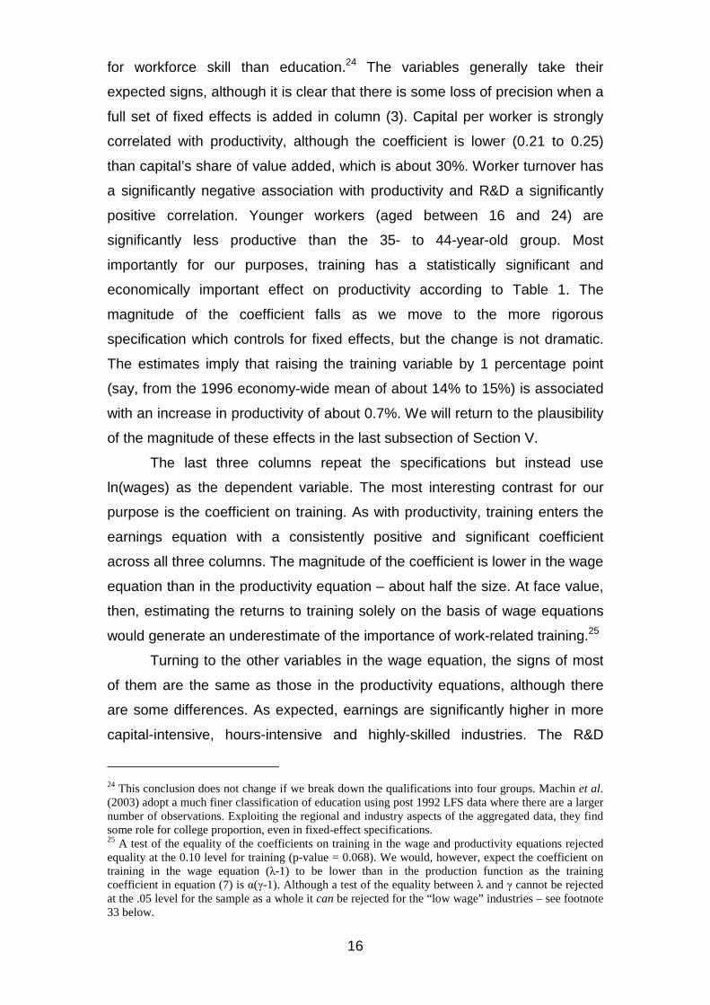
Figure 1 gives the scatterplot of labour productivity (log real value
added per worker) against training propensity and Figure 2 repeats the
exercise for log hourly wages. Not surprisingly, training has a strong positive
correlation with both variables, but the association is somewhat weaker for
wages than for productivity.
The outliers in both graphs tend to be in the service sector.
Unfortunately, the published series for real value added and capital stocks are
rather unreliable in the service sector. For example, in banking and financial
services, measured real value added per person declined every year between
1983 and 1996. Given the poor quality of the service sector production data,
we reluctantly decided to focus the econometric part of the analysis on the
production side of the economy. This is still a substantial share of the
economy – about 50% of private sector net output in 1986.23 Until robust
measures of service sector productivity are developed, there is simply no
alternative to the empirical strategy of focusing on the production sector.
21 Unfortunately, it is not possible to separate out ‘education’ from ‘training’. 22 There is also a question on the length of the training spell, but this was only asked in particular years and there were too many missing values to use it as a separate regressor. Median spell length was two weeks and the mean higher. 23 This led to the loss of only 91 observations and the results are robust to including the service sector in the unweighted regressions. We generally weight the regressions by the number of LFS observations in order to reduce sampling variability. In the weighted regressions, including the service sector does have more substantial effects on the results because of its large employment shares. Full sets of these results are available on request from the authors.
13
Figure 1. Labour productivity and training in British industries
0
1
2
3
4
5
6
0.0
0.1
0.2
0.3
0.4
Proportion training
Lab
ou
r p
rod
uct
ivit
y
Figure 2. Wages and training in British industries
0
0.5
1
1.5
2
2.5
3
0.0
0.1
0.2
0.3
0.4
Proportion training
Wag
es
Notes to Figures 1 and 2: Each point is an industry-year observation. The OLS
regression line has a slope of 4.91 for productivity and 2.95 for wages. Labour productivity is
ln(value added per employee) aggregated from the ACOP and ISDB, wages are ln(hourly
wages) from the ABI and ISDB (wages) and the LFS (hours); training is the proportion of
workers involved in training in the last 4 weeks from the LFS.

14
Care must be taken in interpreting the scatterplots presented in Figures
1 and 2 as they say nothing about the causal impact of training on productivity
or wages. High-training industries are characterised by higher fixed capital
intensity, more professional workers, more educated workers and higher R&D
(see Table A1 in Appendix A). We need to turn to an explicit econometric
model to investigate whether there is a causal effect of training on
productivity, and this forms the focus of the rest of the paper.
V. Results
Baseline industry results
In Table 1, we present the basic results for the industry-level regressions
treating all variables as exogenous. The first three columns have productivity
(log real value added per head) as the dependent variable and the last three
columns have wages as the dependent variable.

15
TABLE 1
Training, productivity and wages
(1) (2) (3) (4) (5) (6) ln(value added per worker) ln(wages) Random effects Random effects Within groups Random effects Random effects Within groups Training .788
(.168) .700
(.169) .696
(.201) .425
(.117) .344
(.119) .365
(.157) ln(capital/worker) .252
(.020) .244
(.019) .212
(.053) .058
(.012) .051
(.012) .069
(.035) ln(hours/worker) .184
(.181) .196
(.181) .275
(.207) .274
(.123) .272
(.126) .310
(.116) Lagged R&D intensity
1.628 (.430)
1.390 (.428)
1.251 (.662)
–.212 (.284)
–.356 (.281)
–.942 (.717)
Worker turnover –.632 (.206)
–.683 (.207)
–.430 (.332)
.132 (.143)
.070 (.145)
.163 (.202)
Occupations: base group is manual workers Managers .487
(.123) .282
(.131) .324
(.084) .195
(.099) Clerical .366
(.174) –.076 (.190)
.161 (.121)
–.126 (.121)
Personal/security –.049 (.355)
–.522 (.371)
.504 (.250)
.204 (.223)
Sales people .443 (.276)
–.078 (.281)
–.037 (.191)
–.328 (.190)
No qualifications –.251 (.096)
–.036 (.109)
.107 (.096)
–.145 (.065)
–.033 (.075)
.101 (.069)
Experience: base group is age 35–44 Age 16–24 –.579
(.170) –.461 (.172)
–.390 (.175)
–.315 (.118)
–.259 (.121)
–.153 (.119)
Age 25–34 –.341 (.155)
–.282 (.158)
–.314 (.171)
–.198 (.109)
–.155 (.110)
–.196 (.111)
Age 45–54 –.058 (.158)
–.042 (.156)
–.104 (.160)
–.139 (.110)
–.148 (.111)
–.150 (.101)
Age 55–64 .178 (.190)
.244 (.192)
.142 (.237)
–.263 (.133)
–.263 (.136)
–.271 (.138)
Male .037 (.097)
.114 (.099)
–.116 (.128)
.293 (.064)
.364 (.065)
–.112 (.078)
Small firm .068 (.112)
.016 (.113)
.005 (.127)
–.118 (.076)
–.126 (.076)
–.056 (.074)
Observations 968 968 968 968 968 968 Estimation period 1984–96 1984–96 1984–96 1984–96 1984–96 1984–96
Notes: Standard errors (robust to heteroskedasticity) are given in parentheses under coefficients. In the first three columns the dependent variable is ln(value added per worker) and in the last three columns the dependent variable is ln(wages). Bold typeface indicates that the variable is significant at the 5% level. All regressions include a full set of regional dummies (10), time dummies (12) and tenure dummies (6). Observations are weighted by number of individuals in an LFS industry cell. Random effects are estimated by GLS. Within groups are estimated by least squares dummy variables (85 industries).
The first two columns are estimated by random effects; the only
difference is that column (1) does not include the occupational controls. This
omission makes some difference to the ‘no qualifications’ variable, which has
a significantly negative association with productivity in column (1) but is
insignificantly different from zero in column (2) – the occupational proportions
(especially the professional/managerial category) do a better job at proxying
16
for workforce skill than education.24 The variables generally take their
expected signs, although it is clear that there is some loss of precision when a
full set of fixed effects is added in column (3). Capital per worker is strongly
correlated with productivity, although the coefficient is lower (0.21 to 0.25)
than capital’s share of value added, which is about 30%. Worker turnover has
a significantly negative association with productivity and R&D a significantly
positive correlation. Younger workers (aged between 16 and 24) are
significantly less productive than the 35- to 44-year-old group. Most
importantly for our purposes, training has a statistically significant and
economically important effect on productivity according to Table 1. The
magnitude of the coefficient falls as we move to the more rigorous
specification which controls for fixed effects, but the change is not dramatic.
The estimates imply that raising the training variable by 1 percentage point
(say, from the 1996 economy-wide mean of about 14% to 15%) is associated
with an increase in productivity of about 0.7%. We will return to the plausibility
of the magnitude of these effects in the last subsection of Section V.
The last three columns repeat the specifications but instead use
ln(wages) as the dependent variable. The most interesting contrast for our
purpose is the coefficient on training. As with productivity, training enters the
earnings equation with a consistently positive and significant coefficient
across all three columns. The magnitude of the coefficient is lower in the wage
equation than in the productivity equation – about half the size. At face value,
then, estimating the returns to training solely on the basis of wage equations
would generate an underestimate of the importance of work-related training.25
Turning to the other variables in the wage equation, the signs of most
of them are the same as those in the productivity equations, although there
are some differences. As expected, earnings are significantly higher in more
capital-intensive, hours-intensive and highly-skilled industries. The R&D
24 This conclusion does not change if we break down the qualifications into four groups. Machin et al. (2003) adopt a much finer classification of education using post 1992 LFS data where there are a larger number of observations. Exploiting the regional and industry aspects of the aggregated data, they find some role for college proportion, even in fixed-effect specifications. 25 A test of the equality of the coefficients on training in the wage and productivity equations rejected equality at the 0.10 level for training (p-value = 0.068). We would, however, expect the coefficient on training in the wage equation (λ-1) to be lower than in the production function as the training coefficient in equation (7) is α(γ-1). Although a test of the equality between λ and γ cannot be rejected at the .05 level for the sample as a whole it can be rejected for the “low wage” industries – see footnote 33 below.

17
coefficient is surprisingly negative (although insignificantly different from zero),
but this turns out to be because of mis-specified dynamics – including longer
lags of R&D demonstrates there is actually a positive correlation of technology
with wages26.
An important concern with Table 1 is that we do not allow for the
endogeneity of training or other suspected endogenous variables. To deal
with this, we implemented the GMM approach described in Section III above.
Table 2 contains a summary of the main results.27 All the same variables are
included in these regressions as in Table 1, but we report only the key
coefficients to preserve space.
In column (1) we present the production function and in column (2) we
present the wage equation. The GMM estimates tell a similar story to the
within-groups estimates. Training has a positive and significant impact on both
productivity and wages, although the training coefficient in the production
function remains almost twice the size of the coefficient in the wage equation
(0.60 vs. 0.35). There are some minor changes to the other coefficients – the
coefficient on capital intensity has risen to 0.33 in the production function, the
R&D coefficient is positively signed in the wage equation and the coefficient
on hours is somewhat larger in magnitude than in Table 1.
26 Consistent with the findings of, inter alia, Bartel and Sicherman (1999). 27 Table B2 in Appendix B has more detailed results, and even more detailed specifications are available from the authors or in Dearden et al. (2000).

18
TABLE 2
Production functions and wage equations estimated by GMM
(1) (2) ln(real value added per worker) ln(wages) Training .602
(.181) .351
(.074)
ln(capital/worker) .327 (.016)
.106 (.011)
ln(hours/worker) .498 (.064)
.489 (.027)
Lagged R&D intensity 1.905 (.262)
.443 (.182)
Proportion of employees who are professionals or managers
.306 (.068)
.160 (.034)
Autocorrelation coefficient (ρ)
.741 (.015)
.797 (.013)
LM1(d.f.) [p-value]
–4.892(85) [0.00]
–6.053(85) [0.00]
LM2(d.f.) [p-value]
–.940(85) [.347]
–1.44(85) [.158]
Sargan(d.f.) 8.819(121) 11.83(146) Instruments (TRAIN)t–2,t–3, ln(Q/N)t–2,t–3,
ln(Hrs/N)t–2,t–3, ln(K/N)t–2,t–3 in differenced equations; ∆(TRAIN)t–1, ∆ln(Hrs/N)t–1, ∆ln(K/N)t–1 in levels equations
(TRAIN)t–3,..,t–5, ln(Q/N)t–3,..,t–5, ln(Hrs/N)t–3,..,t–5, ln(K/N)t–3,..,t–5 in differenced equations; ∆(TRAIN)t–2, ∆ln(Hrs/N)t–2, ∆ln(K/N)t–2 in levels equations
Estimation period 1984–96 1985–96 Observations 898 883 Notes: Estimation by GMM-SYS in Arellano and Bond (1998) DPD-98 package written in GAUSS; one-step robust estimates reported. All regressions include the current values of all the variables in columns (3) and (6) of Table 1 (i.e. turnover, other occupations, qualifications, age, tenure, gender, region, firm size and time dummies). Capital intensity, training, hours and lagged productivity are always treated as endogenous. The other variables are assumed weakly exogenous. One-step standard errors (robust to arbitrary heteroskedasticity and autocorrelation of unknown form) are given in parentheses under coefficients (variables significant at 5% level are in bold). LM1 (LM2) is a Lagrange Multiplier test of first- (second) -order serial correlation distributed N[1,0] under the null (see Arellano and Bond, 1991). Sargan is a Chi-squared test of the over-identifying restrictions. Observations are weighted by number of individuals in an LFS industry cell. Full details in Table B2 in Appendix B.
The diagnostics reported at the base of the table are also satisfactory –
there is no sign of second-order serial correlation (in the first-differences
residuals) and the Sargan test of over-identifying restrictions does not reject.
Note that the wage regression uses instruments dated t–3 and before in the
differenced equation (and dated t–2 in the levels equation). This is because
there were some signs of significant second-order serial correlation using t–2
dated instruments in the wage equation, which invalidates the IVs (we
dropped one period in order to be able to use the longer lags in estimation).

19
Using the (invalid) instruments on the longer time period gave a coefficient
(standard error) on training of 0.141 (0.067) in the wage equation.28
Robustness of the results
We conducted a large number of robustness tests on the models in Tables 1
and 2. Table 3 reports some of these. Given the similarity of the within-groups
and GMM results, we performed these tests on the within-groups
specifications of Table 1, column (3). The first row of Table 3 simply reports
the coefficient and standard error from that column. Using the stock of trained
employees instead of the flow (calculated allowing for depreciation due to
inter-firm turnover) results in very similar results in row 2.29 Keeping only
industries that had 14 continuous years of data (balanced panel) in row 3
means losing 40% of the observations; the coefficient falls, but the change is
not significant (cf. Nickell, 1981). The fourth row includes average wages on
the right-hand side of the production function as a measure of unobserved
worker quality; although wages have a positive coefficient, the training
association remains robust. In row 5 we include all the service sectors,
ignoring our concerns over data quality. The coefficient on training rises to
0.73 and remains significant.
28 Using the shorter time period with longer-dated instruments in the production function gave a coefficient (standard error) on training of 1.043 (0.325). See Table B2 in Appendix B for full details. 29 The non-fixed-effects results were significantly different, but the deviations around the fixed effect in the training stock are dominated by the flow, explaining the similarity of the results. In addition to using the empirical turnover rates, we assumed an exogenous depreciation of training at 40% per annum (see Appendix A). The coefficient was stable to reasonable changes in these parameters (e.g. increasing the depreciation rate to 50% p.a. increased the coefficient to 0.81, to 60% to 0.82; decreasing the depreciation rate to 30% reduced the coefficient to 0.70).

20
TABLE 3
Robustness tests of the production function
Row Robustness test Observations Training coefficient (standard error)
1 Original training coefficient in production sector, Table 1 column (3)
968 0.696(0.201)
2 Using ‘stock’ of trained workers instead of flows 968 0.775(0.189) 3 Using the balanced panel only 572 0.508(0.289) 4 Conditioning on wage in productivity regression (to control
for any residual unobserved worker quality) 968 Training:
0.659(0.219) Wage coeff.: 0.099(0.130)
5 Including service sectors 1,059 0.727(0.206) 6 Include union density (only available 1989–96) 547 Training:
0.604(0.266) Union: –0.177(0.183)
7 Allow all industries to have different training coefficients 968 Mean of heterogeneous coefficients: 0.505
8 Allow non-constant returns 968 0.725(0.201) 9 Estimating a translog production function 968 0.703(0.201) 10 Estimation by non-linear least squares 968 0.518(0.197) 11 Estimation on 1993–2001 data (region–industry cells) 1,873 0.436(0.188) Notes: These all use the specification in column (3) of Table 1 (unless otherwise specified). Estimation by within groups; robust standard errors in parentheses (except row 10). Bold typeface indicates that the variable is significant at the 5% level.
Since training is correlated with unionisation, we could be picking up
‘collective voice’ effects in the main results. Union membership is only
available in LFS since 1989. Despite the loss in sample in row 6, the training
effect is robust to inclusion of union density (density is insignificantly
negatively associated with productivity). In row 7 we allow the training effect to
be different in each of the 85 industries; the mean of these heterogeneous
coefficients is close to the pooled results. The next two rows allow for more
general functional forms, first relaxing constant returns (row 8) and then
estimating a translog production function (row 9); in both cases, the training
coefficient is essentially unchanged. Row 10 gives the results from a non-
linear least squares estimation of equation (8) again showing no significant
difference.
We also compared our results with a recent paper (Machin et al., 2003)
which has built up similar data to our own covering a more recent period and
exploiting the larger size of the LFS post-1992 to construct industry-by-region
cells. Against these advantages, their dataset has a shorter time-series
component (1993–2001) and lacks some of the covariates we use. Re-

21
estimating identical specifications on their dataset gives an estimate of the
training association with productivity of 0.436 with a standard error of 0.188
(see row 11 of Table 3). This is lower, but is still significant and remains well
within two standard errors of our main results.30 On our dataset, we tested
whether there was a tendency for the training coefficient to fall (or rise) over
time in the production function, but we found it to be stable.31
Does the ‘wedge’ between the wage and productivity effect of training
arise from specific human capital or imperfect competition? Under most forms
of imperfect competition, we conjectured that the wedge would be larger in
those industries where workers were earning less than would be implied by
their human capital (i.e. inter-industry wage premiums were low). This could
be because the ‘low-paying’ industries were monopsonistic with large search
frictions or because workers are more able to capture the quasi-rents from
training in the ‘high-paying’ industries.
In order to identify such industries, we used estimates of inter-industry
wage premiums taken from the US Current Population Survey (CPS).32 We
matched the US industries to the UK industries and split the sample at the
median sectoral wage premium. Allowing an interaction between training and
this industry split revealed that the wedge between the training effect on
productivity and the training effect on wages was solely within the ‘low-wage’
industries. To be precise, including an interaction in the wage equation
between training and low-wage industries gave a coefficient (standard error)
of –0.664 (0.196) on the interaction and 0.531 (0.113) on the linear training
effect. In the production function, the interaction was 0.332 (0.297) – positive
but insignificant (the linear training term took a coefficient of 0.612 with a
30 The specification is identical to column (3) of Table 1 except we drop the occupational proportions and R&D and include employment. On our data, this gives a coefficient (standard error) on TRAIN of 0.732 (0.205). 31 For example, interacting TRAIN with a trend in the production function gave a coefficient of 0.003 with a standard error of 0.044. 32 Estimating inter-industry wage premiums from UK wages would have been more problematic as these could reflect endogenous influences – US wage-setting will be driven by the structural characteristics of the industries in question. These US inter-industry wage premiums were generated from individual-level wage regressions from the 1986 CPS Merged Outgoing rotation files. The wage regressions included years of schooling, a quartic in experience, gender, marital status, gender×marriage interactions, race, Standard Metropolitan Statistical Area and regional dummies. The data were kindly provided by Steve Pischke (see Acemoglu and Pischke, 2003, for details).

22
standard error of 0.172)33. In other words, in the ‘high wage premium’
industries, there was no significant difference between the impact of training
on productivity and the impact of training on wages. The fact that our results
are driven by the wedge in low-paying sectors is tentative evidence in favour
of a monopsony/search interpretation.
This evidence is open to the critique that firm-specific training may be
systematically more prevalent in the low-wage sectors (although a priori the
usual view is that ‘good jobs’ are more likely to have more specific skills).
There are several questions in LFS that could be interpreted as general vs.
specific training, so we used them to see if the coefficients differed
significantly with training type – they did not. For example, there are questions
related to off-the-job training (more general) and on-the-job training (more
specific). The proportion of off-the-job training produced a coefficient
(standard error) of 0.005 (0.018) when added to the wage regression and a
coefficient (standard error) of 0.018 (0.029) when added to the production
function. We view this not as any rejection of specific human capital theory per
se, but rather as an indication the type of human capital is intrinsically difficult
to measure. Furthermore, the LFS questions are not asked in all years and
have many missing values.
Quantifying the effects of training
Our key qualitative conclusions are, first, that there is a significant impact of
training on productivity and, second, that the effects of training on productivity
are larger than the effects of training on wages. But, quantitatively, how
economically significant is the magnitude of the training effect?
Interpreting the magnitude of the coefficients is difficult, but the implied
effects are large. From Tables 1 and 2, we conservatively take the coefficient
on training in the productivity regressions to be about 0.6 and the coefficient
on training in the wage regressions to be about 0.3. This would imply that a 10
percentage point increase in the training measure is associated with a 6%
increase in productivity and a 3% increase in wages.
33 A test of the equality between the effects of training on wages (λ) and on productivity (γ) can be rejected at the .05 level for the “low wage” industries (p-value = 0.001), but cannot be rejected for the “high wage” industries (p-value = 0.752).

23
Relative to the returns-to-schooling literature, the training impacts
appear high34. Card (1999) puts the impact of a year of schooling on wages at
about 10%, so our baseline impact of 0.3 is about three times as large. Given
that the typical time in training during the four-week period is under a month
(the median is two weeks, the mean is higher), the returns to a month of
training appear even more impressive. For example, an increase in our key
variable, TRAIN, of 10% would imply a typical worker only spent 5% extra of
his time in training, if training spells were on average two weeks long.
Of course, there may be remaining econometric problems we have not
controlled for generating this difference. But assuming the training effect is not
a statistical artefact, there remain at least two possible explanations for the
training coefficients being larger than conventional estimates of the return to
schooling. First, work-related training may have a higher private return than
schooling as training is more directed at raising productivity in employment.
Training is also likely to have a faster rate of depreciation than schooling, so it
requires a higher year-on-year return in order to give incentives for
investment.35 Second, there may be externalities associated with training that
are missed in the conventional schooling literature, which focuses on private
returns whereas we look at returns to the industry as a whole (cf. Moretti,
2004).
To investigate the externality issue, we estimated some individual-level
wage regressions on the LFS panel. If the private returns to training are higher
than the social returns, we might expect to see a similarly high coefficient in
the individual-level wage regression. We used the individual-level equivalents
of the variables in the industry-level regressions. To construct the proportion
of the year spent in training, we used the LFS panel which follows individuals
for five quarters and asks individuals the training question in each quarter. We
defined a dummy variable (TRAIND4) indicating whether the individual had
been involved in some training in all of the previous four quarters. We also
defined dummies for if the individual had been in training for three quarters
(TRAIND3), two quarters (TRAIND2), one quarter (TRAIND1) or not at all
34 Compared with existing UK estimates of the training effects on wages (e.g. Booth, 1993 and Blundell et al., 1996), our estimates are actually lower (see Dearden et al., 2000, for a detailed comparison). 35 See Heckman et al. (2003) for a recent discussion of interpretation of the schooling coefficient in wage regressions.

24
(TRAIND0). Using TRAIND0 as the omitted base, the results we obtained
from a typical regression were36:
ln( ) 0.165(0.033) 4 0.092(0.023) 3
0.125(0.019) 2 0.078(0.015) 1 controls
wage TRAIND TRAIND
TRAIND TRAIND
= ++ + +
Longer lengths of time in training are associated with significantly higher
wages37. The coefficient on receiving training in all four quarters is 0.165; this
is comparable with the industry-level coefficient of 0.350. Taken literally, this
would suggest that about half of the impact of training on wages at the
industry level is attributable to externalities.
If we include a set of industry dummies (which will include potential
spillovers), the coefficient on TRAIND4 falls from 0.16 to 0.13. If we also
include the initial wage in the first quarter (to control for unobserved
heterogeneity), the coefficient falls even further to 0.079. So these impacts of
a ‘year’ of training are rather similar to the conventional impacts of the returns
to a year in school.
Our conclusion from this exercise is that the larger magnitude of the
training effects in this paper primarily reflects our strategy of estimating at a
level above the individual worker. This was forced upon us by the absence of
adequate data on firm productivity and training, but also because of our desire
to incorporate externalities. The results are therefore consistent with a story
that stresses externalities to training.
Even if there remain econometric problems that have caused us to
overestimate the impact of training at the industry level, it is hard to see why
this would not also bias upwards the training coefficient in the production
function and wage equation to a similar extent. Therefore, even if one
disputes the exact quantitative magnitude of the training effect, our key
qualitative conclusion that the productivity impact of training is greater than
the wage impact should still be valid (this is also a feature of the firm-level
results in Appendix B).
36 Estimation was by OLS; robust standard errors are given in parentheses. Controls include gender, age, areas (20), employer size, occupational dummies (8), no qualification dummy, and a dummy for part-time status. Results are for the production sector only. The quarterly LFS panel 1997–8 was used as two wage observations per individual did not exist in the LFS prior to this. There were 3,998 observations. Full results are available on request from the authors. 37 The training effects are not monotonic. There is even a perverse fall in the coefficient on being in training three relative to two quarters, although the coefficients are not significantly different.

25
VI. Conclusions
In this paper, we have examined the issue of the impact of private sector
training on productivity. Rather than simply use wages as a measure of
productivity, we have presented (for the first time) estimates of the impact of
training on productivity over a long time period. We have assembled a dataset
that aggregates individual-level data on training and establishment data on
productivity and investment into an industry panel covering 1983–96. We
controlled for unobserved heterogeneity and the potential endogeneity of
training using a variety of methods including GMM system estimation.
Using these new data, we have identified a statistically and
economically significant effect of training on productivity in the UK. An
increase of 1 percentage point in the proportion of employees trained is
associated with about a 0.6% increase in productivity and a 0.3% increase in
wages. The impact of training on productivity is robust to a large number of
robustness tests.
We argued that the methodologies in the existing literature may
underestimate the importance of training. The focus on wages as the only
relevant measure of productivity ignores the additional productivity benefits
the firm may capture. The coefficient of training in the production function was
around twice as large as the coefficient in the wage equation. This result could
occur even under standard specific human capital theory. But it could also
arise for a number of other reasons due to imperfect competition in the labour
market (and we have presented some evidence consistent with this
hypothesis). Clearly, further research is needed to distinguish between these
theories.
Finally, a comparison between the industry- and individual-level wage
regressions suggests that our industry-level analysis may capture externalities
from training that are missed out in the micro-level studies. An important
avenue of future research would include probing the returns to training by
combining enterprise data with industry-level data to investigate the
externalities story in greater detail.

26
References
Acemoglu, D. and Angrist, J. (2000). ‘How large are the social returns to education? Evidence from compulsory schooling laws’, NBER Macroeconomics Annual, pp. 9–59.
Acemoglu, D. and Pischke, S. (1999). ‘The structure of wages and investment in general training’, Journal of Political Economy, Vol. 107, pp. 539–572.
Acemoglu, D. and Pischke, S. (2003). ‘Minimum wages and on the job training’, Research in Labor Economics, Vol. 22, pp. 159–202.
Aghion, P. and Howitt, P. (1998). Endogenous Growth Theory, MIT Press, Cambridge, MA.
Arellano, M. and Bond, S. (1991). ‘Some tests of specification for panel data: Monte Carlo evidence and an application to employment equations’, Review of Economic Studies, Vol. 58, pp. 277–297.
Arellano, M. and Bond, S. (1998). ‘Dynamic panel data estimation using DPD for GAUSS’, mimeo, Institute for Fiscal Studies.
Ballot, G. and Taymaz, E. (1998), ‘Firm sponsored training and performance. A comparison Between French and Swedish Firms’, mimeo, ERMES, Paris.
Ballot, G., Fakhfakh, F. and Taymaz, E. (1998). ‘Formation continue, recherche et développement, et performance des entreprises’, Formation Emploi, Vol. 64, pp. 43–55.
Ballot, G., Fakhfakh, F. and Taymaz, E. (2002). ‘Who benefits from training and R&D: the firm or the workers?’, Economic Research Center Working Papers in Economics 02/01, Middle East Technical University, Ankara, Turkey.
Barron, J. M., Black, D. A. and Loewenstein, M. A. (1989). ‘Job matching and on-the-job training’, Journal of Labour Economics, Vol. 7, pp. 1–19.
Bartel, A. P. (1994). ‘Productivity gains from the implementation of employee training programmes’, Industrial Relations, Vol. 33, pp. 411–425.
Bartel, A. P. (1995). ‘Training, wage growth, and job performance: evidence from a company database’, Journal of Labour Economics, Vol. 13, pp. 401–425.
Bartel, A. and Sicherman, N. (1999). ‘Technological change and wages: an inter-industry analysis’, Journal of Political Economy, Vol. 107(2), pp. 285–325.
Barrett, A. and O’Connell, P. (2001). ‘Does training generally work? The returns to in-company training’, Industrial and Labor Relations Review, Vol. 54, pp. 647–683.
Black, S. E. and Lynch, L. M. (1996). ‘Human-capital investments and productivity’, American Economic Review, Vol. 86, pp. 263–267.
Black, S. E. and Lynch, L. M. (2001). ‘How to compete: the impact of workplace practices and information technology on productivity’, Review of Economics and Statistics, Vol. 83, pp. 434–445.

27
Blanchflower, D. and Lynch, L. M. (1992). ‘Training at work: a comparison of US and British youths’, Discussion Paper No. 78, Centre for Economic Performance, London School of Economics.
Blundell, R. and Bond, S. (1998). ‘Initial conditions and moment restrictions in dynamic panel data models’, Journal of Econometrics, Vol. 87, pp. 115–143.
Blundell, R. and Bond, S. (2000). ‘GMM estimation with persistent panel data: an application to production functions’, Econometric Reviews, Vol. 19, pp. 321–340.
Blundell, R., Dearden, L. and Meghir, C. (1996). The Determinants of Work-Related Training in Britain, Institute for Fiscal Studies, London.
Boon, M. and van der Eijken, B. (1997). ‘Employee training and productivity in Dutch manufacturing firms’, Research paper no. 9716, Department of Statistical Methods, Statistics Netherlands, Voorburg.
Booth, A. (1991). ‘Job-related formal training: who receives it and what is it worth?’, Oxford Bulletin of Economics and Statistics, Vol. 53, pp. 281–294.
Booth, A. (1993). ‘Private sector training and graduate earnings’, Review of Economics and Statistics, Vol. 75, pp. 164–170.
Booth, A., Francesconi, M. and Zoega, G. (1999). ‘Training, rent sharing and unions’, mimeo, University of Essex.
Card, D. (1999). ‘The causal effect of education on earnings’, in O. Ashenfelter and D. Card (eds), Handbook of Labour Economics, Elsevier, Amsterdam.
Carriou, Y. and Jeger, F. (1997). ‘La formation continue dans les entreprises et son retour sur investissement’, Economie et Statistique, Vol. 303, pp. 45–58.
Dearden, L., Reed, H. and Van Reenen, J. (2000). ‘Who gains when workers train? Training and corporate productivity in a panel of British industries’, Working Paper No. 00/04, Institute for Fiscal Studies.
De Koning, J. (1994). ‘Evaluating training at the company level’, in R. McNabb and K. Whitfield (eds), The Market for Training, Avebury, Aldershot.
Delame, E. and Kramarz, F. (1997). ‘Entreprises et formation continue’, Economie et Prevision, Vol. 127, pp. 63–82.
Green, F. and Steedman, H. (1997). Into the Twenty First Century: An Assessment of British Skill Profiles and Prospects, Special Report, Centre for Economic Performance, London School of Economics, London.
Greenhalgh, C. (2002). ‘Adult vocational training in France and Britain’, Fiscal Studies, Vol. 23, pp. 223–263.
Greenhalgh, C. and Stewart, M. (1987). ‘The effects and determinants of training’, Oxford Bulletin of Economics and Statistics, Vol. 49, pp. 171–189.
Griliches, Z. (1992). ‘The search for R&D spillovers’, Scandinavian Journal of Economics, Vol. 94, pp. S29–S47.
Grunfeld, D. and Griliches, Z. (1960). ‘Is aggregation necessarily bad?’, Review of Economics and Statistics, Vol. 42, pp. 1–13.

28
Hægeland, T. and Klette, T. (1999). ‘Do higher wages reflect higher productivity? Education, gender and experience premiums in a matched plant-worker data set’, in J. Haltiwanger, J. Lane, J. R. Spletzer, J. Theeuwes and K. Troske (eds), The Creation and Analysis of Employer–Employee Matched Data, Amsterdam, North Holland.
Haskel, J., Hawkes, D. and Pereira, S. (2003). ‘Skills, productivity in the UK using matched establishment, worker and workforce data’, Ceriba, Discussion Paper, May.
Heckman, J., Lochner, L. and Todd, P. (2003). ‘Fifty years of Mincer earnings regressions’, National Bureau of Economic Research, Working Paper No. 9732.
Hellerstein, J. and Neumark, D. (1999). ‘Sex, wages and productivity: an empirical analysis of Israeli firm level data’, International Economic Review, Vol. 40, pp. 95–123.
Hellerstein, J., Neumark, D. and Troske, K. (1999). ‘Wages, productivity and worker characteristics: evidence from plant level production functions and wage equations’, Journal of Labor Economics, Vol. 17, pp. 409–446.
Holzer, H. (1990) ‘The determinants of employee productivity and earnings’, Industrial Relations, Vol. 29, pp. 403–422.
Holzer, H., Block, R., Cheatham, M. and Knott, J. (1993). ‘Are training subsidies for firms effective?’, Industrial and Labor Relations Review, Vol. 46, pp. 625–636.
Ichniowski, C., Shaw, K. and Prennushi, G. (1997). ‘The effects of human resource management practices on productivity’, American Economic Review, Vol. 87, pp. 291–313.
Jones, P. (2001). ‘Are educated workers really more productive?’, Journal of Development Economics, Vol. 64, pp. 57–79.
Krueger, A. and Rouse, C. (1998). ‘The effects of workplace education on earnings, turnover and job performance’, Journal of Labor Economics, Vol. 16, pp. 61–94.
Lazear, E. (1979). ‘Why is there mandatory retirement?’, Journal of Political Economy, Vol. 87, pp. 1261–1284.
Lillard, L. A. and Tan, H. W. (1992). ‘Private sector training: who gets it and what are its effects?’, Research in Labour Economics, Vol. 13, pp. 1–62.
Lynch, L. M. (1992). ‘Private sector training and the earnings of young workers’, American Economic Review, Vol. 82, pp. 299–312.
Machin, S., Vignoles, A. and Galindo-Rueda, F. (2003). Sectoral and Area Analysis of the Economic Effects of Qualifications and Basic Skills, Research Report No. RR465, Department for Education and Skills, London
Moretti, E. (2004). ‘Workers’ education, spillovers and productivity: evidence from Plant-Level Production Functions’, American Economic Review, Vol. 94, pp. 656–690.
National Skills Task Force (1998). Towards a National Skills Agenda, Department for Education and Employment, Sudbury.

29
Nickell, S. J. (1981). ‘Biases in dynamic models with fixed effects’, Econometrica, Vol. 49, pp. 1417–1426.
O’Mahony, M. (1998). ‘Anglo-German productivity differences: the role of broad capital’, Bulletin of Economic Research, Vol. 50, pp. 19–36.
Winkelmann, R. (1994). ‘Training, earnings and mobility in Germany’, Discussion Paper No. 982, Centre for Economic Policy Research.

30
Appendix A. Data
Data construction for industry panel
The database we construct combines several sources. The critical individual-
level source is UK Labour Force Survey (LFS). LFS is a large-scale
household interview-based survey of individuals in the UK which has been
carried out on varying bases since 1975.38 Around 60,000 households have
been interviewed per survey since 1984. The LFS data are useful for our
purposes as they contain detailed information on:
• the extent and types of training undertaken by employees in the survey;
• personal characteristics of interviewees (e.g. age, sex, region);
• the skills of individuals (educational qualifications and occupation);
• some basic workplace characteristics (e.g. employer size, industry);
• job characteristics of employees (e.g. job tenure, hours of work).
We work with this information aggregated into proportions and/or
averages by (broadly) three-digit SIC80 industry. Our sample includes all
employed men and women aged between 16 and 64 inclusive (i.e. employees
plus the self-employed) for whom there was information on the industry under
which their employment was classified.
The main training question asked to employees in the Labour Force
Survey between 1983 and 1996 was ‘over the 4 weeks ending Sunday …
have you taken part in any education or training connected with your job, or a
job that you might be able to do in the future … ?’. Figure A1 presents the
average proportions of employees undertaking training in each year of the
LFS sample and shows a reasonably steady increase in the 1980s.39 From
1990 onwards, the proportion of employees receiving training stabilises at
around 14% and stays at or around this level for the rest of the sample period.
38 Between 1975 and 1983, the survey was conducted every two years. From 1984 until 1991, it was conducted annually. Since 1992, the Labour Force Survey has been conducted every three months in a five-quarter rolling panel format. 39 It should be noted that the figure of around 5% for 1983 is almost certainly an underestimate because in 1983 the four-week training question was only asked of employees under 50, whereas in all subsequent years it was asked of employees over 50 and under 65 as well. However, even if the training measure is calculated as the proportion of employees aged under 50 receiving training in every year, the figure for 1983 is still lower than that for 1984.

31
Figure A1. Overall training incidence, Labour Force Survey, 1983–96
0
0.05
0.1
0.15
0.2
1983
1984
1985
1986
1987
1988
1989
1990
1991
1992
1993
1994
1995
1996
Year
Pro
po
rtio
n r
ecei
vin
g t
rain
ing
in la
st 4
wee
ks
We did some simple decomposition analyses to investigate whether the
increase in aggregate training was due to the growth in size of industries that
are (and always have been) relatively more training intensive. It turns out that
this is only a minor factor: over 95% of the increase in aggregate training is
due to an increase within a large number of different sectors.40 This is
consistent with the findings of other papers, which have found that the
aggregate growth of education or occupational skills is essentially a within-
industry phenomenon (e.g. Machin and Van Reenen, 1998).
LFS also has further information on the type of training received
(although not all of the questions on this are asked in each year). For
example, the questionnaire distinguishes between ‘on-the-job’ training (e.g.
learning by example and practice while doing the job) and ‘off-the-job’ training
(training conducted as a formal training course). Whilst the incidence of on-
the-job training reported in LFS has been more or less constant since the mid-
1980s, the proportion of workers receiving some off-the-job training in the four
weeks prior to being surveyed rose from about 5% in 1984 to 8% in the early
40 The change of training propensity over a given period can be decomposed into a within-industry and
a between-industry component: ii
iii
i STTST ∑∑ ∆+∆=∆ where Ti = proportion of workers in
industry i undertaking training, S = share of industry i in total employment, a bar denotes a mean over time and delta is the difference over the given period.

32
1990s. Other indicators of training (not asked in every year) include the
duration of training, whether it was employer funded and whether it was
completed or still ongoing. We examined whether there were differential
productivity effects for all these different types of training, but could find no
significantly different coefficients.41
The second major dataset we use is the Annual Census of Production
(ACOP). This gives production statistics on capital, labour and output for
industries in the manufacturing, energy and water sectors (collectively known
as the production sector of the economy). It is based on the ARD (Annual
Respondents Database), which is a survey of all production establishments
(plants) in the UK with 100 or more employees, plus a subset of
establishments with less than 100 employees. We use the ACOP data on
value added, gross output, investment, employment and wages for industries
in the manufacturing sector and the energy and water industries.
Capital stocks were calculated using the perpetual inventory method
drawing on NIESR’s estimates of initial capital stocks (see O’Mahony and
Oulton, 1990). All the nominal measures were deflated with three-digit
industry price indices from the ONS. For the services industries, we drew on
the ISDB (InterSectoral DataBase) compiled by the OECD.
There was a change in SIC classification in 1992 which forced us to
aggregate some of the industries and prevented us from using some of the
industries after the change. Additionally, we insisted on having at least 25
individuals in each cell in each year. After matching the aggregated individual
data from LFS, we were left with 94 industry groupings over (a maximum of)
14 years (85 in the production sectors).42
Means of the variables are given in Table A1 broken down by high- and
low-training industries.
41 The measure of training used takes no account of the intensity or length of the training course (except in so far as a longer training course is more likely to fall within the four-week period prior to the survey). There is some evidence that the length of training has been falling since the later 1980s (for a detailed analysis, see Felstead et al., 1997). However, when we estimate training effects separately for each year of the LFS sample, the magnitude of the training effect does not differ significantly over time. One might expect a decrease in the productivity effect of the training measure for the later years if the average quality of training courses had declined (there was no evidence of this in our data). 42 Full details on how the data were constructe can be obtained from the authors or in Dearden et al. (2000).

33
Calculating the training stock
The main results use the flow in training, but we also report some experiments
with an estimate of the stock of trained workers in an industry. If we define the
stock of people who have been trained in the industry at time t as NTt and the
flow as MTt then if the stock evolves according to the standard perpetual
inventory formula, it can be expressed as
NTt = MT
t + (1–δ) NTt–1
where δ is the rate at which the stock of effectively trained workers at time t
decay in their productive usefulness by time t+1. This training depreciation
rate represents several things. First, individuals will move away from the
industry, so their training can no longer contribute to the industry’s human
capital stock. Second, the usefulness of training will decline over time as old
knowledge becomes obsolete and people forget (e.g. knowledge of the DOS
operating system). Third, to the extent that training is firm specific, turnover
between firms in the same industry may reduce industry productivity. Although
we obtain some measures of turnover using the LFS, the second element of
depreciation is essentially unknown. Because of this uncertainty, our baseline
results simply use the proportion of workers trained in an industry (TRAIN in
equation (3) in Section II). This will be equal to the stock when δ=1.
Nevertheless, we also estimate the training stock. We use the average worker
turnover rate as one element of depreciation and then add an extra
‘exogenous element’ varying between 0.2 and 0.6. We also need to make an
assumption about the initial stock in 1983. We assume that the steady-state
growth, rate of the training stock g is 2% per annum, which enables a first-
year approximation of the stock as MT83/(g+δ). The qualitative results are quite
robust over different measures.43
Firm-level data
The firm-level data are based on the ‘Survey on Human Resource Practices
and Corporate Value in the Modern Corporation’ conducted in 1996 by Martin
Conyon (see Conyon and Reed, 1999). The relevant training variable was
q23f: ‘How have the following training strategies used by your company

34
changed between 1990 and 1995 … The percentage of company sales
turnover spent on training has increased/decreased/not changed’. The
number of firms giving some response to this question was 135. We matched
this survey to company accounting data from Datastream (data between 1968
and 1997). We discarded firms with missing values on the training and
accounting variables, leaving us with a sample of 119 companies.
Productivity was measured by real sales (Datastream Item 104) per
worker (Item 219). Capital is the historical book value (Item 330) and wages
were estimated as total remuneration (Item 215) divided by the number of
workers (Item 219). All accounts are consolidated.
43 See the discussion around row 2 of Table 3 in the main text. We also considered looking at the inflows of trained workers from other industries to improve the stock measure, but the LFS sample of industry switchers was too small to construct the full three-digit flow matrix.

35
TABLE A1
Means of variables by high- and low-training industries
Variable Mean, low-training industries
Mean, high-training industries
Proportion of male employees 62.4% 80.9% Proportion aged: 16–24 22.7% 15.5% 25–34 24.5% 25.4% 35–44 22.2% 24.0% 45–54 19.1% 22.1% 55–64 11.1% 12.8% Proportion in occupation: professional/managerial 14.7% 27.1% Clerical 8.5% 10.9% personal/security 1.9% 1.6% salesforce/technical 3.4% 2.5% other occupations 71.5% 58.0% Highest qualification: degree 2.6% 7.3% sub-degree level 3.7% 9.2% A level / equivalent 15.5% 22.5% O level / equivalent 15.6% 14.3% other/none/missing 62.7% 46.7% Tenure in current job: less than 6 months 10.9% 7.1% 6 months – 1 year 8.4% 5.8% 1 year – 2 years 11.1% 8.0% 2 years – 5 years 21.6% 17.8% 5 years – 10 years 18.8% 19.7% 10 years – 20 years 18.0% 24.3% more than 20 years 9.0% 16.5% Proportion in small firm 21.2% 12.6% Average ln(capital–labour ratio) 2.22 3.02 Average ln(real value added per worker) 2.76 3.19 Average ln(gross output per worker) 3.80 4.27 Average ln(hourly wages) 1.56 1.84 Average hours worked 39.1 40.2 Average R&D spend as proportion of output 0.52 2.99 Note: ‘High-training’ industries are those that trained on average more than 8.7% of employees (the sample median).
Appendix B. Additional results
Some firm-level results
As a preliminary investigation of the impact of training on productivity, we
turned to the only UK dataset we know of that combines training data and
objective productivity measures at the firm level. We constructed this by
combining a firm survey with company accounting data from Datastream (see
Appendix A for details). We estimated an OLS production function in long
differences with results summarised in Table B1. The drawback of the firm-
level training data is that we only know whether a firm increased the

36
percentage of turnover allocated to training over this time period and not the
actual quantitative change, so the table is simply illustrative.
Columns (1) and (2) of Table B1 give results for productivity and
columns (3) and (4) have the results for wages. Columns (2) and (4) condition
on industry dummies. In columns (1) and (3), the indicator for the change in
training is positively and significantly associated with both productivity
changes and with wage changes. Interestingly, the magnitude of the
association with productivity is about twice as large as the magnitude of the
association with wages. We uncovered a similar finding when we examined
the industry-level data.44 A second feature of Table B1 is that much of the
association between training, productivity and wages is due to industry-level
(growth) effects. When sector dummies are added, the coefficient on training
falls by half in the productivity regression (second column) and by three-
quarters in the wage equation (fourth column). The training effects are no
longer significant. This implies that a substantial element of the training
correlation is due to industry growth effects. It is these changes over a much
longer time period that we exploited in the main part of the paper.45
More detailed industry results
Table B2 reports the unrestricted coefficient estimates underlying Table 2 in
the main text and the restricted estimates of the production function
parameters after imposing the COMFAC restrictions. If we took the
unrestricted coefficients, our preferred models in columns (1) and (4) would
suggest a larger magnitude of the long-run impact of training on productivity46
(2.289) than of training on wages (1.529). The qualitative finding that the
productivity effect is twice the size of the wage effect remains unaltered.
44 Given the size of the sample, it is not surprising that the difference in training coefficients is not significant (p-value=0.23, allowing for cross-equation correlation of the errors through SUR). 45 In the spirit of looking for complementarities (Ichniowski et al., 1997), we investigated allowing for interactions between changes in training and changes in many other features of the firm – merit pay across four different skill groups, employee involvement, retention, flexibility, three types of delayering, share options, teamwork, competition, etc. With the exception of merit pay for managers (which was significant at the 10% level), none of these interactions was statistically significant. It is worth noting that neither Black and Lynch (1997) nor Bartel (1995) find strong evidence of such interactions in their data. 46 i.e. using )1/()( 132 πππ −+ in the context of equation (14) in Section III.

37
TABLE B1
Training, productivity and wages at the firm level (long differences, 1995 - 1990)
(1) (2) (3) (4)
Dependent variable: Mean change in ln(sales per worker) Mean change in ln(average wage)
Growth in training as a percentage of turnover
.021 (.009)
.010 (.010)
.012 (.006)
.003 (.007)
Mean change in ln(capital per worker)
.139 (.045)
.159 (.049)
.066 (.032)
.103 (.033)
Sector dummies (32) No Yes No Yes
Observations 119 119 119 119
R2 .41 .62 .22 .63
Notes: Estimation by OLS in long differences (average 1995 - 1990); robust standard errors under coefficients. Bold typeface indicates that the variable is significant at the 5% level. All regressions include controls for the growth in employment and whether there was an increase in the proportion of skills (four groups: managers, clerical, skilled manual, unskilled manual), of females and of part-timers. These are all continuous variables. ‘Growth in training as a percentage of turnover’ is a dummy variable indicating whether training grew as a percentage of turnover between 1990 and 1995.

38
TABLE B2
Detailed GMM results (1) (2) (3) (4)
ln(real value added per worker) ln(wages) Constrained – COMFAC imposed Training .602
(.181) 1.043 (.182)
.141 (.067)
.351 (.074)
ln(capital/worker) .327 (.016)
.325 (.017)
.188 (.006)
.106 (.011)
ln(hours/worker) .498 (.064)
.519 (.062)
.518 (.031)
.489 (.027)
Lagged R&D intensity
1.905 (.262)
1.538 (.340)
.226 (.159)
.443 (.182)
Proportion of employees who are professionals or managers
.306 (.068)
.337 (.074)
.230 (.028)
.160 (.034)
Years 1984–96 1985–96 1984–96 1985–96 NT 898 833 898 883 Autocorrelation coefficient (ρ)
.741 (.015)
.758 (.014)
.822 (.009)
.797 (.013)
LM1(d.f.) [p-value]
–4.892(85) [0.00]
–4.513(85) [0.00]
–5.444(85) [0.00]
–6.053(85) [0.00]
LM2(d.f.) [p-value]
–.940(85) [.347]
–.674(85) [.500]
–2.003 [.045]
–1.44(85) [.158]
Sargan (d.f.) 8.819(121) 6.605(146) 11.03(121) 11.83(146) Instruments (TRAIN)t–2,t–3,
ln(Q/N)t–2,t–3, ln(Hrs/N)t–2,t–3, ln(K/N)t–2,t–3 in differenced equations; ∆(TRAIN)t–1, ∆ln(Hrs/N)t–1, ∆ln(K/N)t–1 in levels equations
(TRAIN)t–3,..,t–5, ln(Q/N)t–3,..,t–5, ln(Hrs/N)t–3,..,t–5, ln(K/N)t–3,..,t–5 in differenced equations; ∆(TRAIN)t–2, ∆ln(Hrs/N)t–2, ∆ln(K/N)t–2 in levels equations
(same as column 1) (TRAIN)t–2,t–3, ln(Q/N)t–2,t–3, ln(Hrs/N)t–2,t–3, ln(K/N)t–2,t–3 in differenced equations; ∆(TRAIN)t–1, ∆ln(Hrs/N)t–1, ∆ln(K/N)t–1 in levels equations
(same as column 2) (TRAIN)t–3,..,t–5, ln(Q/N)t–3,..,t–5, ln(Hrs/N)t–3,..,t–5, ln(K/N)t–3,..,t–5 in differenced equations; ∆(TRAIN)t–2, ∆ln(Hrs/N)t–2, ∆ln(K/N)t–2 in levels equations
Unconstrained – COMFAC not imposed Lagged dependent variable
.543 (.058)
.599 (.063)
.707 (.035)
.624 (.045)
Trainingt .930 (.465)
.652 (.412)
.248 (.165)
.303 (.149)
Trainingt–1 .116 (.241)
–.969 (.648)
–.085 (.134)
.272 (.289)
ln(capital/worker)t .278 (.073)
.323 (.056)
.120 (.051)
.028 (.037)
ln(capital/worker)t–1 –.156 (.063)
–.104 (.063)
–.078 (.044)
.020 (.033)
ln(hours/worker)t .495 (.165)
.434 (.123)
.359 (.064)
.480 (.079)
ln(hours/worker)t–1 –.422 (.231)
–.397 (.169)
–.189 (.114)
–.362 (.100)
R&D intensityt–1 1.248 (.605)
1.137 (.669)
.549 (.323)
.551 (.334)
R&D intensityt–2 –1.157 (.673)
–.671 (.740)
–.493 (.311)
.592 (.354)
Managerial proportiont
.446 (.129)
.392 (.136)
.125 (.056)
.113 (.070)
Managerial proportiont–1
–.148 (.129)
–.173 (.113)
–.044 (.087)
–.054 (.088)

39
Notes: This table reports a fuller set of results than those in Table 2 (which correspond to columns (1) and (4) of Table B2). Estimation by GMM-SYS in Arellano and Bond (1998) DPD-98 package written in GAUSS. All regressions include the current values of all the variables in columns (3) and (6) of Table 1 (i.e. turnover, other occupations, qualifications, age, tenure, gender, region, firm size and time dummies). Capital intensity, training, hours and lagged productivity are always treated as endogenous. The other variables are assumed weakly exogenous. One-step standard errors (robust to arbitrary heteroskedasticity and autocorrelation of unknown form) are given in parentheses under coefficients. LM1 (LM2) is a Lagrange Multiplier test of first- (second-)order serial correlation distributed N[1,0] under the null (see Arellano and Bond, 1991). Sargan is a Chi-squared test of the over-identifying restrictions. Observations are weighted by number of individuals in an LFS industry cell.