Stockholm2004-02-06

MASTER THESIS

Mathematical statisticsAnd

Numerical analysis

Longstaff and Schwartz models for American Options

By

Göran Svensson

Department of mathematicsRoyal Institute of TechnologyS-100 44 Stockholm, Sweden

2

Abstract

This thesis consists of two parts. In the first part the Longstaff and Schwartz least squaresmethod (a Monte-Carlo method) for pricing American type options is investigated. Themethod is based on valuation through a comparison between the value of early exercise and theconditional expected value of continued possession. The result is regressed on a set of basisfunctions. In this paper the functions are simple polynomials. The results is compared to theresults from a finite difference scheme and proves to be reliable.In the second part of the thesis a finite element model is implemented to solve a two factorpartial differential equation model, known as the Longstaff and Schwartz two factorequilibrium model. The implementation is first tested against an analytical solution for asimple bond and is then used to price a floorlet (as an example).The model is then expanded with a successive over relaxation solver that can handle obstacleproblems to price American type derivatives. An American put option on a bond is priced andcompared with the value of a European put option on the same bond and with the samematurity.

3

INDEX

1 Introduction 41.1 Some interest rate derivatives 4

2 A least square Monte-Carlo method for the pricing of American options 62.1.1 L-S one factor model for pricing American options 62.1.2 The LSM algorithm 72.1.3 Convergence results 82.2 Implementation of a one-factor model 82.2.1 Implementation 82.2.2 Results and validation 10

3 L-S two factor equilibrium model 133.1.1 Model 133.1.2 The Longstaff and Schwartz PDE 143.2 Implementation of the finite element method163.2.1 Boundary conditions 163.2.2 The analytical solution for Bonds and European derivatives 183.2.3 Numerical solution using FEM 193.2.4 The grid 213.2.5 Implementation of the model and simple validations 223.2.6 Comparison between analytical and FEM models for the price of a bond 233.2.7 Limitations of the implemented model 253.3 Results 263.3.1 Floors and floorlets 263.3.2 American and European put option on a bond 27

4 Discussion 29Appendix A 30Bibliography 31

4

1 Introduction

One of the fastest growing markets in recent years has been the interest rate derivativesmarket. This makes it more and more important to develop accurate models for pricing thesetypes of financial instruments. Many models in use are one factor models. The problem withthese models is that they sometimes fail to capture the complexities of interest rate behaviour.Therefore the importance of generating good multifactor models has increased. The main goalof this thesis is to study and implement one such model, the Longstaff and Schwartz (L-S)two factor interest rate equilibrium model.

It is somewhat harder to price interest rate derivatives than similar stock derivatives becauseof several reasons. Firstly the pay-off is not always as simple to model as for stocks, since itoften is done at several times during the life time of the option. For example a floor has anumber of periodic pay-off dates. Another factor is the dependence on the whole termstructure for the interest rate. These factors are addressed by L-S in their model, which usesthe short term interest rate and the volatility of the short term rate as the two factors. It is anequilibrium model which has been derived from an idealised economy. It can however betransformed into an arbitrage free model with a few simple manipulations [7].

In this thesis the L-S two factor model (TFM) is implement and studied. The implementationhas been done by using a finite element method (FEM) to compute a numerical solution. Thischoice is motivated by the variational calculus that is well suited to calculate the price for bothEuropean and American contracts. First for a simple bond and then for a floorlet. There areanalytical solutions for the bond which makes it easy to verify if the model produces correctresults. As a natural expansion of the implementation a solver that can handle obstacleproblems is included. This allows for the pricing of American type derivatives. For Americanoptions there exist no analytical solution, therefore other tests are necessary.

The first part of this project will have the form of a smaller study treating the efficiency of theL-S least square method (LSM) for pricing American options. This method uses conditionalexpectation of the value of continued possession of the option versus the immediate exercisevalue. One of the main advantages of this method is that it is a Monte-Carlo method which canhandle American options. This valuation method could be extended to handle TFM and then itwould be possible to test the results from the obstacle solver of the FEM model (which is notdone due to lack of time).

1.1 Some interest rate derivatives

As stated above, this paper mainly treats interest rate contingent claims. Below is a short listof some major types of interest rate derivatives.

Bond optionsA bond option gives the owner the right to buy or sell a particular bond at a certain price at

5

specific points in time. One common occurrence of bond options are in an embedded form.That means that the buyer of a bond also receives a bond option. Pricing European bond

options is normally straight forward and can be done analytically with a plethora of models.To accommodate American (Bermudan) style options, numerical methods are normally used.An American put option on a bond will be priced later on.

SwaptionsWhich is short for swap options. This is an increasingly popular form of options on interestrates. It is an option that gives the holder the right to enter into a swap with a specific interestrate, at certain times in the future. They can be traded both as European or American(Bermudan) options. For the former there exists several analytical models for evaluation whileone needs to resort to other methods to price the latter.

Caps/FloorsAn interest rate cap protects the holder from floating interest rising above a certain level. Thecap works in the following manner, the cap comes with a cap rate which is periodicallycompared to the floating rate i.e. London inter bank offered rates (LIBOR). If the floating rateis greater than the cap rate then the option pays the difference times the principal. Thepayment is received at the end of the period, just at the time of the next comparison. Thesetime periods are called tenors and the option for just one tenor is known as a caplet. The floorworks in the same manner as the cap but it pays money when the floating rate goes below thefloor rate, it offers protection against low floating rates. The option for one such tenor isknown as a floorlet. If one can price a caplet or a floorlet it is straight forward to extend it toany cap or floor (each caplet/floorlet has to be priced separately). One interest rate derivativethat will be priced in this paper is a floorlet. To accomplish this, initial conditions andboundary conditions will be needed. In the following section one set of boundary conditionswill be explored.

6

2 A least square Monte-Carlo method for the pricing of American options

L-S uses a LSM and conditional expectations to price American contingent claims. The basicvaluation framework is the general derivative pricing model put forth by Black, Scholes andMerton (and others), according to L-S [10].

2.1.1 L-S one factor model for pricing American options

First we need to introduce the state space, W, which is the set of all possible states of thestochastic economy in the finite time period [0, T]. A specific sample path is represented byw. Let ¡ be the sigma field of distinguishable events at time T and let P be the probabilitymeasure defined on ¡. Then we have a complete probability space (W, ¡, P) and on top of thiswe assume the existence of an equivalent martingale measure Q.

The value of an American option equals the maximized value of the discounted cash flowsfrom the option, where the maximum is taken over all discernible stopping times as given bythe filtration F = {¡t; t Œ [0, T]}, that is the Snell envelope. Introduce the following notation;C(w, s; t, T) to denote different paths generated by the option which has not been exercisedprior to or at time t. It is also assumed that the holder of the option follows the optimalstopping strategy for all s, t < s £ T.

The objective of the L-S least squares pricing method is to approximate the optional stoppingrule for each path that maximizes the value of the option. To make simulation possible letthere be K discrete exercise times, 0 < t1 £ t2 £ ... £ tK = T and consider the optimal stoppingrule at each date. In reality American type derivatives are often continuously exercisable; theLSM algorithm can approximate this fact if K is taken to be sufficiently large. At theexpiration date the owner receives the final pay-off from the option as usual. At other allowedexercise times the owner needs to choose between continued possession of the option andearly exercise.

At each time tj (j = 1, 2, ..., K-1) the value of immediate exercise is known by the holder whilethe value of continuation is not know. From standard no-arbitrage valuation theory we knowthat the value of holding on to the option is given by the expected value of the discounted cashflows up to time T, that is C(w, s; tj, T), with respect to the risk-neutral measure Q. At time tj

the value of continuation, F(w; tj) can be expressed as [10]

)1.2(|),;,(),(exp);(1 ˙

˙˚

˘

ÍÍÎ

È¡˜

˜¯

ˆÁÁË

Ê-= Â Ú

+=

K

jk

t

t

t

jjk

k

j

Qj TttCdssrEtF www

where r is the riskless discount rate and at each time tj the expectation is taken conditionallyon the filtration ¡t(j). If, at any given exercise date, the value of immediate exercise is higher

7

than the conditionally expected value of continuation, that option should be taken.

2.1.2 The LSM algorithm

It is apparent from the name that this method uses a least squares approach to approximatethe conditional expectation function at times tj (j = 1, 2, ..., K-1). In the solution process, onestarts at the final value and work our way backwards through the different cash flows, C(w, s;t, T). At tK-1 it is assumed that the unknown functional form of F(w; tK-1) in equation (2.1) canbe represented by a linear combination of the countable set of ¡t(K-1)-measurable basicfunctions. The assumption is justified when the conditional expectation is an element in L2.Since L2 is a Hilbert space it has a countable orthonormal basis and so the conditionalexpectation can be represented as a linear function of the elements in this basis. Whenapplying this to a real problem one has to limit oneself to a finite number of basis functions.Let M < • be the number of basis functions in the chosen orthonormal basis [10].

At the final exercise date tK, the path-wise cash-flows of the option are known, which makesit possible to calculate C(w, s; tK-1, T), the cash-flows after time tK-1

1. Then approximate F(w; tK-1) using least squares and an orthonormal basis. This is done by regressing the cash-flows C(w, s; tK-1, T) on the M basis functions for the in-the-money paths. Then this value iscompared with the value of immediate exercise to decide on the optimal stopping rule for timetK-1. Once this has been calculated the value at time tK-1 is known which makes it possible todo it all over again for the time tK-2. By repeating this procedure one will gain optimalstopping rules for all times and trajectories. By discounting all cash-flows in the final cash-flow matrix C(w, s; 0, T) and averaging over all paths gives an approximation of the value ofthe option [10].

Main algorithm;

i) Simulate N paths wi of the state variables.

ii) Calculate the value of the option at expiry for all paths wi .

iii) Use the cash flow matrix C(wi, s; tK-1, T) to find an estimate of the conditional expected value of continuation (find an estimate of F(w, tK-1)). Only consider in-the-money paths.

iv) Compare with the value of immediate exercise to get a stopping rule (when to stop foroptimal results).

v) Determine the new cash flow matrix C(wi, s; tK-2, T), using the above exercise decisions.

1 We are only interested in paths that are in-the-money. The reasons for including only in-the-money cash flowsare as L-S state "We use only in-the-money paths since it allows us to better estimate the conditional expectationfunction in the region where exercise is relevant and significantly improves the efficiency of the algorithm" [10].

8

vi) Do this recursively for all exercise dates

vii) Sum all discounted cash flows and average them to approximate the option value.

2.1.3 Convergence results

L-S show that the LSM-algorithm is convergent, this is done via two propositions which theyprove [10]. Intuitively their results state that with a sufficient number of basis functions, M,and a large number of random samples, N -> •, the LSM-algorithm converges to the solutionwith any desired level of accuracy e.

2.2 Implementation of a one-factor model

The intent is to use the L-S LSM method to price American types of derivatives on interestrate in a two factor framework. Before using this method as a basis for comparison it shouldbe tested to see if it really generates believable results and to investigate what kind of basisfunctions are to be used. This study will be based entirely on numerical results for the onedimensional case. In their article (Longstaff and Schwartz, "Valuing American Options bySimulation: A Simple Least-Squares Approach", 1999) L-S claim that numerical tests showthat the pricing method is convergent for basis functions as simple as powers of the statevariables (simple polynomials). In the next section a polynomial of the state variable (X) willbe picked and examined to see if the results are good enough to approximate the value of anAmerican option.

2.2.1 Implementation

The implementation of the LSM-algorithm described above is done in Matlab and can best beunderstood through a schematic overview of the solution process2 (see schematic on nextpage). First the matrix with the random samples is created. After that the cash flow matrix isinitialised with the terminal date pay-offs. Then the process of recursive valuation (whilegoing back in time) is started. The first step is always to find the value of the underlyingcommodity (stock in this case) and from that information calculate which trajectories are to beused (that is which paths are in-the-money) in the regression. If there are any trajectories in-the-money the regression process is started so that the conditional expectation value ofcontinued possession can be calculated and compared to the value of immediate exercise.Then the cash flow matrix is updated with any new cash flows. This process continues untilthe initial date of the contract is reached. Then the discounts that corresponds to the differentcash flow times are calculated and applied. The final step is to average over all trajectories to

2 For a good numerical example see [10].

9

obtain the approximate value of the option.

Schematic for the lsm program

Create matrix with monte carlo paths

t(i)=t(n)=T

Initialize the Cash-flow matrix with final date pay-offst(i)=t(n-1)

Calculate underlying values for all trajectories

Find the trajectories that are in-the-money (IDM), their position and their value

If IDM > 0 if IDM=0

Make regression on chosen basisfunction (chosen polynomial)

t(i)=t(i-1)

Calculate the maximum expectedvalue and determine the optimal

exercise time. If earlyexercise record the value

if t(i)>0Update the cash-flow matrix with optimal values

if t(i) = 0

Find all discounts and apply them

Calculate the final value by averaging over all trajectories

Where the terminal time T = t(n) and the initial time t = t(0) is the time when the recursiveprocess is stopped and all results are added.

Study of polynomialsL-S chose the three first terms of the Laguerre polynomial as basis function. This choice willbe compared with simple polynomials of the form

10

( ) 2210 XaXaaXP ++=

and3

32

210)( XaXaXaaXP +++=

and with a finite difference solution.

2.2.2 Results and validation

First one needs to decide on the basis function to use for regression. As stated above mainlybasis functions in the form of polynomials will be used. Firstly some test results usingdifferent degrees of polynomials and different numbers of random trajectories is show in table1.Table 1.

Number oftrajectories

polynomialdegree 1

polynomialdegree 2

polynomialdegree 3

polynomialdegree 4

polynomialdegree 5

10 7.78 8.67 7.87 7.02 8.35

100 6.21 6.88 5.74 6.50 7.49

500 6.15 6.09 6.32 6.41 6.59

1000 6.34 5.97 5.93 5.80 6.51

5000 6.07 6.07 5.96 6.00 6.08

10000 5.96 6.05 6.13 6.08 6.09

Price of an American put with strike price of K=40, expiry date T=1 (that is one year from today), the volatilityof the stock is 40% and the interest rate is considered fixed at 6% (continuous). The number of exercice dateswas 50 and the initial stock price used was 38.

As can be seen from table 1, the solutions become more and more convergent towards thebottom right corner. The price seems to be approximately 6.10 for this option. Which is closeto both the finite difference solution and the Laguerre polynomial solution.A comparison with another basis function (the first three Laguerre polynomials) but with thesame method is done in table 2. The same American put option is also evaluated using a finitedifference scheme (in the Black and scholes framework).

Table 2.

S0 Finite diff. Laguerre 2:nd order 3:rd order

36 7.17 7.09 6.87 6.97

38 6.19 6.13 6.05 6.13

40 5.33 5.31 5.11 5.16

42 4.63 4.59 4.41 4.51

44 3.97 3.97 3.89 3.94

Price of an American put with strike price of K=40, expiry date T=1 (that is one year from today), the volatility

11

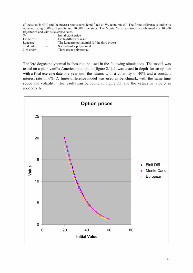
of the stock is 40% and the interest rate is considered fixed at 6% (continuous). The finite difference solution isobtained using 1000 grid points and 10.000 time steps. The Monte Carlo solutions are obtained via 10.000trajectories and with 50 exercise dates.S0 - Initial stock priceFinite diff. - Finite difference resultLaguerre - The Laguerre polynomial (of the third order)2:nd order - Second order polynomial3:rd order - Third order polynomial

The 3:rd degree polynomial is chosen to be used in the following simulations. The model wastested on a plain vanilla American put option (figure 2.1). It was tested in depth for an optionwith a final exercise date one year into the future, with a volatility of 40% and a constantinterest rate of 6%. A finite difference model was used as benchmark, with the same timescope and volatility. The results can be found in figure 2.1 and the values in table 3 inappendix A.

Option prices

0

5

10

15

20

25

0 20 40 60 80

Initial Value

Val

ue Finit Diff

Monte Carlo

European

12

Figure 2.1 Comparison between the results from a finite difference scheme, using 1000 grid-points and 10000time-steps, and the Monte-Carlo based simulation used 10000 trajectories with 50 exercise opportunities. Thevolatility of the underlying stock was 40%, the strike-price of 40, the maturity of one year and the interest wasset at 6% (continuous). Also a plain European put option is shown, with the same maturity, interest rate andvolatility. The values for the European option was calculated using the Black and Scholes formula.

The two models are in fairly good agreement. The Monte Carlo model seems to under valuethe option somewhat, which is what the L-S paper predicts. A few other tests where made,with fewer initial values for the underlying stock. The results were similar to the ones obtainedabove. It is concluded that this could be used as a test for American type options (it wasmeant to be used as a test for the model implemented in the next chapter, but time was notsufficient to make the comparison in a meaningful way).

13

3 L-S two factor equilibrium model

In many cases the one factor interest rate models fail to accurately describe the interest ratedynamics. Then it can be necessary to turn to multifactor models for better precision. Thechoice of factors depends on what kind of financial instrument is being priced. Generally thefirst factor in interest rate models is the spot rate (short term interest rate). L-S chose thevariance of the interest rate as the second factor of their model. This will not affect bondpricing to any great extent but does have a significant impact on option pricing. The followingaccounts observed option pricing [6]

( )( )2.3),,(

1.3),(),,(

2

1

dzdttVrdV

dztrVdttVrdr

VV

r

sm

m

+=

+=

There are two stochastic processes, dz1 and dz2, involved. Here r is the short term interestrate, V the volatility of r and the m:s are the drift factors. This is the way the L-S model workswhen applied to pricing. The background for the model is however an idealised economy. Themodel of the L-S economy is in itself not useful or realistic. It is intended for the calculation ofinterest rate derivatives rather than to calculate term structures and the prices of bonds(according to R. Rebonato) [12].

3.1.1 Model

The idealised L-S economy [6] consists of identical companies that produce a single good. Ateach point in time the participants of this economy can choose between investing orconsuming the good. All investors are considered rational and interested in maximizing theirutility of the single good produced. Let C(t) be the consumption at time t, then all participantsin the economy try to maximize, subject to budget constraints, his/her additive preferences ofthe form

( ) ( )3.3)(ln)exp( ˙̊˘

ÍÎÈ -Ú

•

tt dssCsE r

where r is the utility discount function from s to present day t. A consumer maximizes thisexpectation based on the available information up to time t, of the value of future discountedconsumption. This means is that some part of the amount of the single good an investorpossesses today can be reinvested to gain even more amounts in the future or it can beconsumed to receive "happiness" today. L-S assume a logarithmic utility function. Then it ispossible to represent the change in wealth as

( )4.3dtCQ

dQWdW -=

14

where the returns of investments in the production process is given by (dQ/Q) andconsumption of goods is represented by -Cdt. W is the current wealth invested. The returns

from an investment is not certain and is therefore represented by a stochastic differentialequation of the form

( )5.3)( 1dzYdtYXQ

dQsqm ++=

where dz1 is the normal increment of a Brownian motion, m, q and s are constants. X and Yare state variables of the economy model chosen so that X is unrelated to the productionuncertainty (dz1) and Y is the factor that is correlated to the production process. X and Y areWiener processes and can be described by the following stochastic differential equations [6]

( )( )7.3)(

6.3)(

3

2

dzYfdteYddY

dzXcdtbXadX

+-=

+-=

where a, b, c, d, e ,f > 0, and z2 and z3 are scalar Wiener processes. z2 is independent from z1

and z3. These stochastic processes do not represent any obvious phenomena in the real world.Their use is justified by the fact that they make the model tractable.

If one accepts rW as the optimal consumption one obtains the following stochastic equationdescribing the wealth process

( )8.3)( 1dzYWdtWYXdW srqm +-+=

3.1.2 The Longstaff and Schwartz PDE

W,X and Y form a joint Markov process, the values of these variables completely describe thegiven economy and the future returns on investments. If one rescale the state variables so thatx = c-2X and y = f--2Y and let H(x, y, t) denote the value process of the contingent claim withmaturity t. L-S use the following PDE [6]

( )9.3)),()(()(22 2

2

2

2

t

HrH

y

HYWCov

J

Jy

x

Hx

y

Hy

x

Hx

W

WW

∂

∂=-

∂

∂---+

∂

∂-+

∂

∂+

∂

∂xhdg

where g = a c-2, x = e, d = b, h = d f--2, r is the instantaneous riskless rate and Cov(W,Y) is theinstantaneous covariance of changes in W with respect to changes in Y. The investor derivedutility of the wealth function is partially separable and has the form

15

( ) ( ) ( )10.3),,(lnexp

),,,( tYXGWt

tYXWJ +-

=r

r

The market price of risk is connected to the utility dependent term in the coefficient of Hy

which in turn is dependent on the production uncertainty of Y. Because of the separable form

of the derived utility of the wealth function it can be shown that

( )11.3),( yYWCovJ

J

W

WW l=˜̃¯

ˆÁÁË

Ê -

where l is constant and l represents the market price of risk. The risk premium is determinedinside the model, depending on the model parameters, which are in some way obtained fromthe real world. Thus the price of risk is set endogenously and therefore the model is consistentwith non-arbitrage models [7]. A separation of variables results in an analytical solution forEuropean type derivatives which can be priced once the initial rate r, boundary- and initial-conditions have been determined. Equation (3.9) becomes

( )12.3)()(22 2

2

2

2

t

HrH

y

Hy

x

Hx

y

Hy

x

Hx

∂

∂=-

∂

∂-+

∂

∂-+

∂

∂+

∂

∂uhdg

where n = x + l.

Unfortunately the prices are set in terms of the state variables of x and y and not in observablevariables. With some manipulation of the model one can however transform the price so thatthe price can be expressed in terms of two realistic variables, such as the short term interestrate, r and the variance thereof, V.

To relate the short term interest rate to the expected change in marginal utility one can useBreeden (1986), according to L-S [6]. Because of the logarithmic structure of the utility of thewealth function, the short term interest rate is simply the expected return minus the varianceof production returns. Which takes the following form in the L-S framework

( )13.3yxr ba +=

where a = mc2 and b = (q - s2)f2. The variance of the riskless interest rate can then becalculated to be

( )14.322 yxV ba +=

where both r and V are positive for all feasible state variables. provided that a and b are notequal the system has an unique solution in terms of the state variables x and y. By invertingthe two equations above one obtains

16

( )( )15.3

abab

-

-=

Vrx

( )( )16.3

abba-

-=

rVy

This mapping allows the transformation from r and V to x and y.

3.2 Implementation of the finite element method

The pay-off structure of interest rate derivatives are dependent on the level of some interestrate. Since these types of contingent claims are becoming both more popular and morespecialized, the task of pricing them has become more important. The pricing procedure ofinterest rate instruments is made more complex due to several factors. One of the moreimportant ones is the discounting procedure, since interest is both used for discounting and todefine the pay-off. To value many products the whole yield structure must be modeled andalong the yield curve the volatility can vary significantly. This is one reason for using a modelwith two parameters, one which represents the short term interest and the other thatcorresponds to the volatility of the interest.

3.2.1 Boundary conditions

The use of Blacks model to obtain boundary conditions is somewhat naive, but the boundariesare complex due to the transformation of variables and due to the fact that the implementationin this thesis does not accept state variables that are negative (see figure 3.1 or section 3.2.7for a more complete description of the problem).

The pay-off from a floorlet corresponding to the rate observed at time tk and paid at time tk+1

is

( ) ( )17.30,max kXk RRL -d

where RX is the floor rate and Rk is the floating rate. L is the principal (L = 1 will be used inthis paper) and dk = tk+1 - tk. Then Blacks model states that the value of a floorlet will be [3]

( ) ( ) ( )[ ] ( )18.3,0 121 dNRdNRtPL kXkk ---+d

where P(0,tk+1) is the zero coupon bond paying 1 unit at time tk+1. The zero coupon for a floorwill be constructed step by step as each floorlet is priced. To obtain the final result onesimply has to add the price (present value) of all the floorlets to get the price of the completefloor. N(.) is the cumulative probability distribution function for a variable that is normallydistributed with a mean of zero and a variance of one. And finally

17

( ) ( )19.32ln 2

1

kk

kkXk

t

tRRd

s

s+=

( )20.312 kk tdd s-=

where dk is the volatility for the period tk to tk+1. RX and Rk are expressed with compoundingfrequency corresponding to the tenor length.

European Boundary ConditionsThe boundary conditions for European contingent claims are the Black prices, obtained via themodel described above and the plug in of the interest rate and the volatility at the point on theboundary in question, i.e. if one point on the boundary corresponds to an interest rate of 6%and a volatility of 2% then those values are put into Blacks formula to obtain the boundaryvalue at that point. These boundary conditions are used on boundaries 1-3 in figure 3.1. Onthe fourth boundary a Dirichlet condition has been used.

18

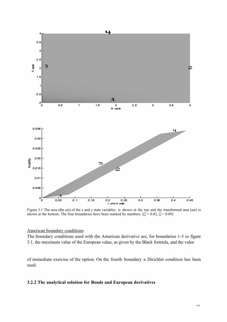
Figure 3.1 The area (the set) of the x and y state variables is shown at the top and the transformed area (set) isshown at the bottom. The four boundaries have been marked by numbers. (a = 0.02, b = 0.09)

American boundary conditionsThe boundary conditions used with the American derivative are, for boundaries 1-3 in figure3.1, the maximum value of the European value, as given by the Black formula, and the value

of immediate exercise of the option. On the fourth boundary a Dirichlet condition has beenused.

3.2.2 The analytical solution for Bonds and European derivatives

19

To price interest rate derivatives it is necessary to model the basic interest rate. This isnormally done in one of two ways. One category of models are the non-arbitrage models,where all prices are calculated using risk neutral evaluation (under different measures). Theother type of models are the so called equilibrium models. Both these types have advantagesand disadvantages. The L-S model is an equilibrium model but can be transformed into anarbitrage free model as L-S shows in their article "A two-factor interest rate model andcontingent claims valuation" [7]. In this article they also show how one can price differentinterest rate derivatives in an analytical fashion. The basis for the analytical model is equation3.12 which is solved by separation of variables. This gives a powerful tool for valuation.

The value of a European interest contingent claim is equal to its forward price multiplied bythe value of a unit-discount bond with the same maturity. Both the contingent claim and thezero coupon bond must obey equation 3.12. The general pay-off function at maturity will be

( ) ( ) ( )21.3,0,, yxGyxH =

One can divide the value function H(x,y,t) into two parts,

( ) ( ) ( ) ( )22.3,,,,,, tyxMtyxFtyxH ¥=

where F(x,y,t) is the unit-discount bond (zero coupon bond). Since F(.) will be equal to one atthe terminal date, what is left is

( ) ( ) ( )23.3,0,, yxGyxM =

Which can be solved using a separation of variables approach according to L-S [6,7].

If M is taken to be one then all that is left is the zero coupon bond and an analytical solutioncan be found [6]

( ) ( ) ( ) ( ) ( )( ) ( )24.3exp,, 22 VtDrtCttBtAtVrF ++= khg

where

( )( ) ( )( )

( )25.321exp

2

fffdf

+-+=

ttA

( )( ) ( )( )

( )26.321exp

2

yyyuy

+-+=

ttB

( ) ( )( ) ( ) ( )( ) ( )( )

( )27.31exp1exp

abfy

fbyyaf

-

---=

tAttBttC

( ) ( )( ) ( ) ( )( ) ( )( )

( )28.31exp1exp

abfy

yffy

-

---=

tBttAttD

20

and

( )29.3lxu +=

( )30.32 2daf +=

( )31.32 2uby +=

( ) ( ) ( )32.3yuhfdgk +++=

This explicit formula will be used to validate the FEM model, to check for convergence. Onehas to ask what the advantages are of a numerical model compared to the analytical? The mostobvious one is that the analytical model does not allow for pricing of American typeinstruments while the numerical model can be extended by an obstacle solver to handleAmerican options. In this paper a successive over relaxation solver is implemented [5]. Thisextension of the model will make it possible to price American options.

3.2.3 Numerical solution using FEM

To numerically solve a partial differential equation (PDE) one needs to use a method that isrobust and reliable. The finite element method is such a method, it is well suited to diffusion-advection problems. First the variational form of the main equation has to be constructed usingan appropriate test function. Using Galerkins [5] method to choose the approximation used.Since it is a two factor model it will correspond to a two dimensional implementation of theFEM. This will be done using triangular elements on an unstructured grid. To finally obtainresults one needs to input initial conditions (e.g. terminal pay-off from a given instrument) andto find appropriate boundary conditions.

The main equation is (3.12)

( )12.3)()(22 2

2

2

2

t

HrH

y

Hy

x

Hx

y

Hy

x

Hx

∂

∂=-

∂

∂-+

∂

∂-+

∂

∂+

∂

∂uhdg

which is given us in the state-space of x and y. Assume that H belongs to the subspace P

( )33.3),,( PŒtyxH

then introduce a test function, g, that is of the same subspace as H

( )34.3),( PŒyxg

21

Which leads to the variational form

( )35.30)()(22 2

2

2

2

ÚÚ =˙˚

˘ÍÎ

È

∂

∂--

∂

∂-+

∂

∂-+

∂

∂+

∂

∂

t

HrH

y

Hy

x

Hx

y

Hy

x

Hxgdydx uhdg

Partially integrate to remove the equation of the second derivatives and then introduce thelinear FEM approximation with

( ) ( )36.3,),(1Â =

=N

j jj yxhyxH f

( ){ } ( )37.3,,1,),( Niyxyxg i K="Πf

where hj is the value of H(x,y,t) in that specific grid point at time t. This is the Galerkin choiceof a test function. The space discretisation is then combined with a partly implicit timediscretisation

( )38.3)()1()( tSttSt

hh tj

ttj qq -+D+=

D

-D+

( )39.31,2

1˙̊˘

ÍÎ

ÈŒq

Where Dt is the time step and S(t+Dt) and S(t) are the discretized equations on the grid at thecorresponding times. The complete discretized FEM equation then takes the following form

( ) ( ) ( ) ( )( ) ( ) ( ) +—-—+——ÍÎ

ÈÁË

Ê +—+——Â ÚÚ jxijyijyiyj jxijxix

yxdydx fgfffffffff

2

1

22

1

2

( ) ( ) ( ) ) ] =+D++—+—-—+ D+ ttjjijijijyijyijxi htyxyx ffqffbffaffnfhfffd

( ) ( ) ( ) ( )( ) ( ) ( )Â ÚÚÍ

Î

È—+—-——-Á

Ë

Ê —-——-=j

jxijyijyiyjxijxix

yxdydx fgfffffffff

2

1

22

1

2

( ) ( ) ( ) )( ) ] ( )40.31 tjjijijijyijyijxi htyxyx ffqffbffaffnfhfffd +D---—-—+—-

where —i is the partial derivative with respect to the variable i. In short one can write this inmatrix form and obtain

( )41.3tjij

ttjij hBhA =D+

22

In the implementation of the model the integrals are calculated with quadratures on anunstructured triangular grid.

The quadratures used to approximate the integrals over the triangular grid are

( ) ( )42.30rfAfdS totªÚ

D

( ) ( ) ( )( ) ( )43.3

3

1321Ú

D

++ª qfqfqfAfdS tot

( ) ( ) ( )[ ] ( )44.32783

60

10Ú Â Â

D

++ªi j jitot rfqfpfAfdS

Where Atot is the total area over the triangular element. Equation (3.42) integrates exactly overlinear problems, equation (3.43) integrates exactly over quadratic problems and where equation(3.44) integrates exactly over cubic problems. This means that terms like rH are the mostcomplex to solve (they become cubic integrals).

3.2.4 The grid

The area is divided into triangular elements over which the equation is solved. The grid isgenerated with Matlabs grid generator (in the PDE toolbox). The grid in x and y state variableslook as follows

23

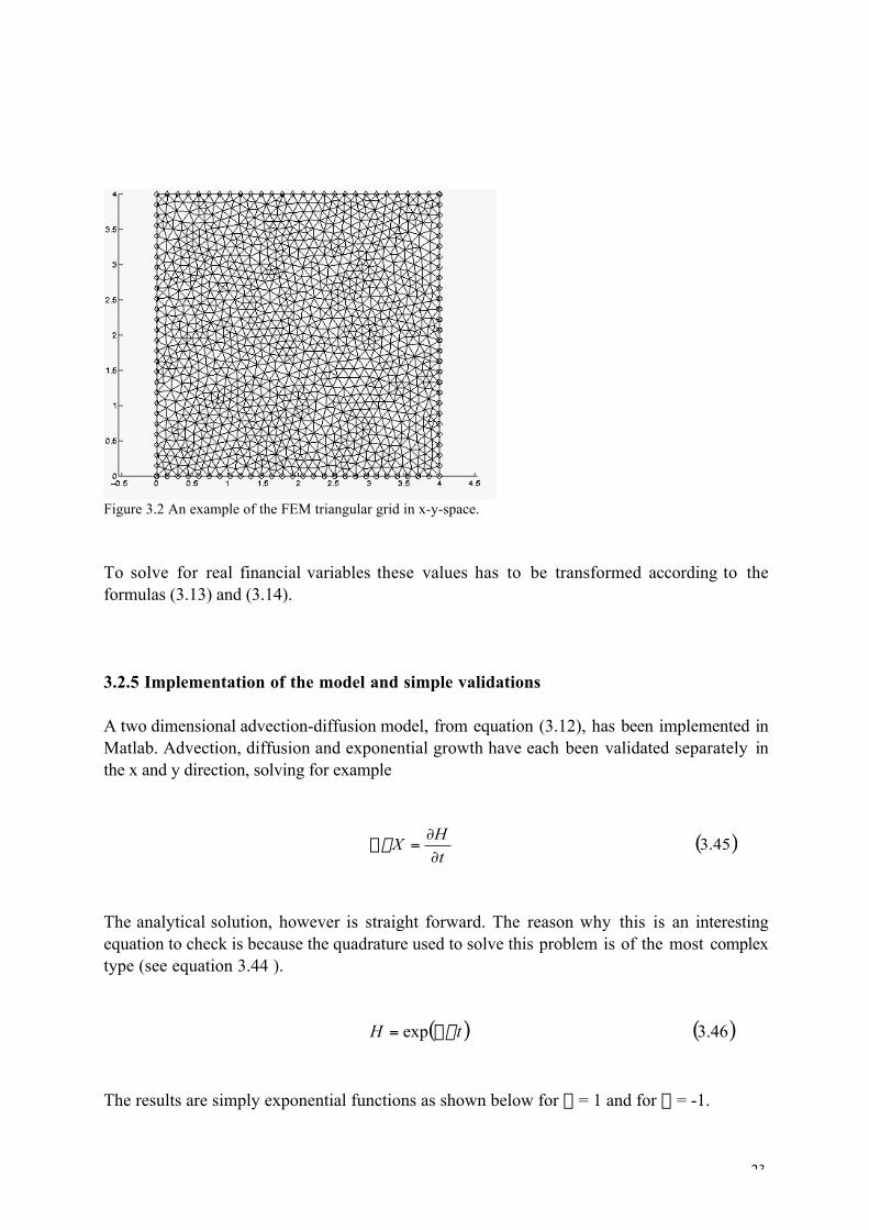
Figure 3.2 An example of the FEM triangular grid in x-y-space.

To solve for real financial variables these values has to be transformed according to theformulas (3.13) and (3.14).

3.2.5 Implementation of the model and simple validations

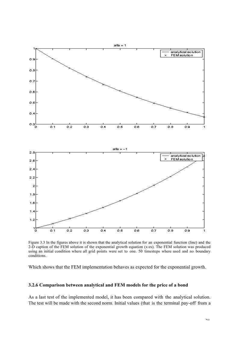
A two dimensional advection-diffusion model, from equation (3.12), has been implemented inMatlab. Advection, diffusion and exponential growth have each been validated separately inthe x and y direction, solving for example

( )45.3

t

HX

∂

∂=-a

The analytical solution, however is straight forward. The reason why this is an interestingequation to check is because the quadrature used to solve this problem is of the most complextype (see equation 3.44 ).

( ) ( )46.3exp tH a-=

The results are simply exponential functions as shown below for a = 1 and for a = -1.

24

Figure 3.3 In the figures above it is shown that the analytical solution for an exponential function (line) and the2-D caption of the FEM solution of the exponential growth equation (x:es). The FEM solution was producedusing an initial condition where all grid points were set to one. 50 timesteps where used and no boundaryconditions.

Which shows that the FEM implementation behaves as expected for the exponential growth.

3.2.6 Comparison between analytical and FEM models for the price of a bond

As a last test of the implemented model, it has been compared with the analytical solution.The test will be made with the second norm. Initial values (that is the terminal pay-off from a

25

zero coupon bond) for the computer model are 1, since that is the risk-free amount that willbe paid at the last date of the zero coupon bond. The boundary conditions are calculated usingthe analytical solution at all points on the boundary. See figure 3.4 for convergence results.

Figure 3.4 Which shows the 2-norm vs. (number of elements)-1 . The 2-norm was calculated as

ÂÂ -22

analyticalFEManalytical

As can be seen in figure 3.4, the size of the error decreases as more elements are included in themodel, which is the desired behaviour. One slight worry is that the result does not seem to go

26

down to zero, only to a small number. It could perhaps be explained with the differentsolution methods (separation of variables versus FEM)..

3.2.7 Limitations of the implemented model

As mentioned above the model is built around the two state-variables, x and y. Equation (3.12)is solved in the x and y-space in the L-S model (of the short term interest rate). The x and yvariables can be transformed into the observable variables r and V, which corresponds to theshort term interest rate and the volatility thereof. This transformation is dependent on the aand b parameters. These parameters are obtained from either historical data analysis or fromthe implications of existing option prices. This means that the transformation from x and y tor and V is determined by factors in the financial market. Which limits the domain over which itis possible to calculate option prices with the model implemented in this paper (see fig. 3.1 foran illustration).

Can this limitation be overcome? The most obvious way to try to overcome this problem is toextend the domain in x and y-space to include negative numbers as well. This would thenextend the domain in r and V-space to include all possible values for the short interest rate andthe volatility thereof. It is however clear that negative x and y result in anti-diffusion and theFEM quickly becomes unstable. This is a serious limitation to the implemented FEM model.It does limit both the areas where the financial variables are calculable and it forces artificialboundary conditions on the FEM (see boundary conditions in section 3.2.1).

27

3.3 Results

The model is built around two state-variables, x and y, which do not correspond to anymeasurable financial data but can be transformed into real world observables. This leads tosome limitations applicability of the model. The boundary conditions have to match the state-variables which limits the values obtained if the boundary conditions are not well chosen.After having implemented the FEM of the L-S short term interest rate model, it is applied tothe valuation of a floorlet (as an example). The solution procedure can then be extended toprice a floor of any length by multiple uses of the implemented model (and knowledge aboutdiscount rates). This is done by simply adding the results from all payment periods (tenors).The model parameters will then be changed to demonstrate the effects on the price underdifferent circumstances. Finally the model is extended to include a solver which handlesAmerican style contingent claims. As an example a plain vanilla put option on a bond will bevalued.

3.3.1 Floors and floorlets

Having implemented the model and decided on the initial and boundary conditions to use, it istime to start using the model to obtain values (prices) under different circumstances. Theinitial conditions, pay-offs, are particularly important for the pricing of derivatives. For stockoptions the pay-off functions are straight forward and can easily be handled, but for interestrate derivatives the pay-off function normally consists of several cash-flows at different times.To successfully price such instruments one need a full set of discount rates (zero couponbonds or similar sources that corresponds to the term structure). The pricing process willinvolve adding the discounted prices for all reset periods of the derivative.

In the following section a floorlet with a three month tenor will be studied. The period that isexamined is the period that begins three months into the future, when the floating interest ratefor that tenor is set. At the end of the second tenor the payment is due. The volatility is fixedat 2.5%, while the short rate is allowed to vary and is shown on the x-axis. To produce thegraphical results from the FEM implementation the value at the centre of each triangularelement in the path of the chosen volatility (that is elements that lies on the fixed volatilityline) has been used.

The prices of different products with the same maturities depend strongly on the parametersthat are plugged into the model. These parameters can be obtained via implied calculation orfrom historical data [6,8,12]. Large d and n tend to make the FEM implementation unstable,particularly at the boundaries. Large in this case means d > 2 and n > 1. These terms have astrong effect on the solutions obtained. For low values of d and n the value of thecorresponding derivative becomes high even though the volatility is low (see fig. 3.5). Figure3.5 shows the price of two different floorlets. The boundary conditions are as described insection 3.2.1 under European boundary conditions.

28

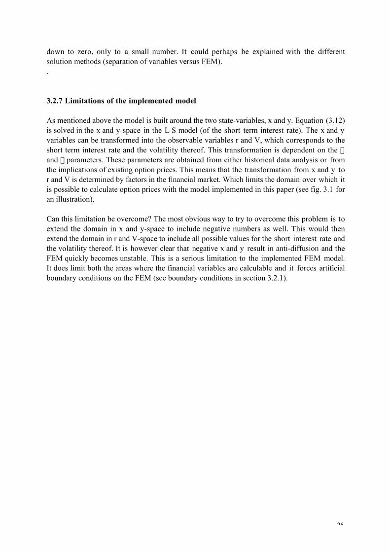
Figure 3.5 Two different sets of parameters on floorlets with the same maturities and strike prices. The floorletshave a three month tenor when the floating interest rate is fixed and payment occurs at the end of the secondthree month tenor. The strike price K=0.06. Solution one corresponds to the following set of parameters a =0.02, b = 0.09, g = 1.2, d = 0.008, h = 0.20, n = 0.0008, q = 0.50 ,while solution 2 corresponds to a = 0.02,b = 0.09, g = 0.0560, d = 0.30648, h = 0.23017, n = 0.2689, q = 0.50, volatility = 0.0025. Number of time-steps used for both solutions where 25.

It can clearly be seen that different parameter values have a great impact on the solution. Thisis one of the strengths of the model, a wide variety interest rate behaviours can be described. Italso makes parameter estimation extremely important.

3.3.2 American and European put option on a bond

29

The final product that will be studied is a plain bond option but of an American type, whichmeans that it can not be priced in an analytical fashion. In the implementation of the L-Smodel a solver for obstacle problems has been included. It is (as mentioned above) a successiveover relaxation (SOR) solver (implemented from [5]).American bond options are not traded on open markets (nor are European ones) but they areoften included in other over-the-counter (OTC) contracts. Loans and deposits often containembedded bond options. A deposit that can be redeemed without penalty at any time (after acertain time) contains an American (Bermudan) put option on a bond [3]. Similarly the loancommitment from a financial institution (bank or other) is an American put option on a bond.

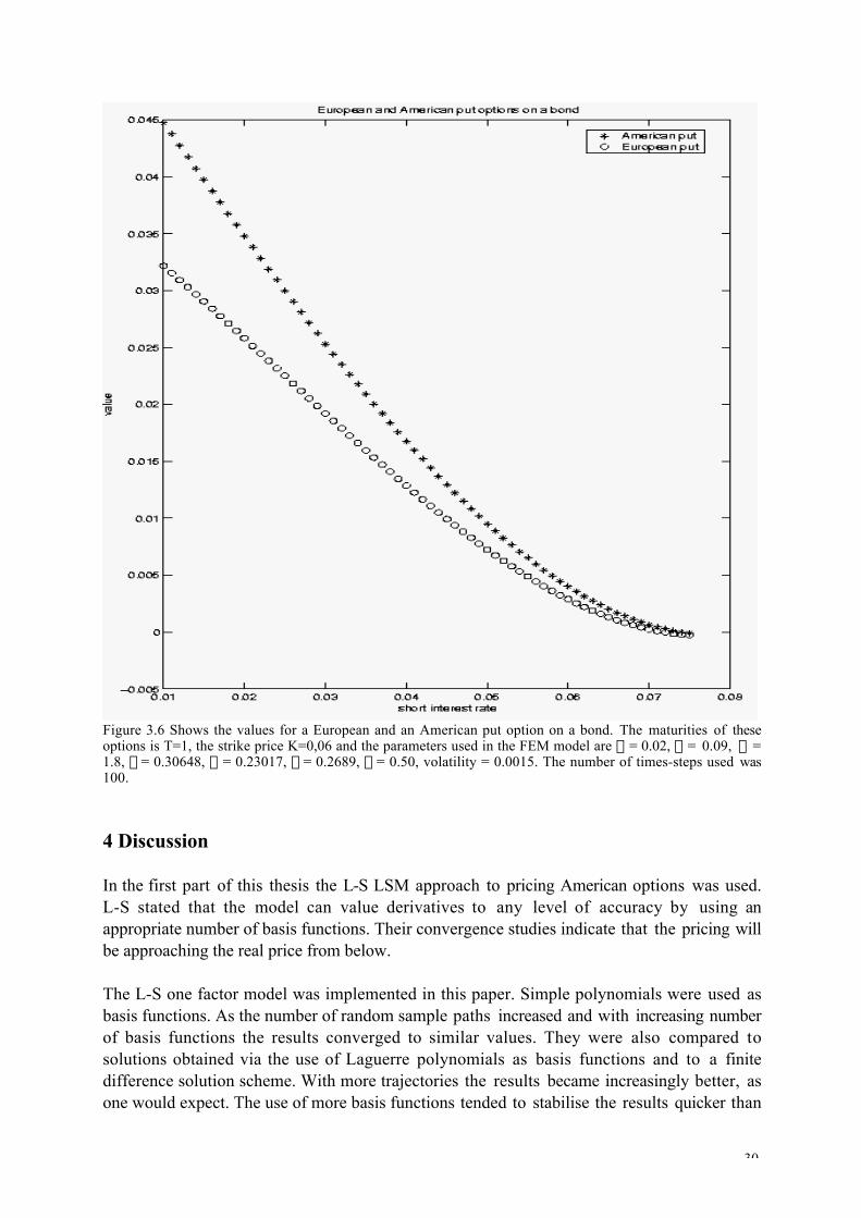
Since these types of loans, mortgages and deposits are very common it is good to be able tovalue these embedded options. Another nice feature is that they also have simple pay-offstructures, which makes it easier to price them via a PDE model such as the L-S two factormodel. In figure 3.6 a comparison is made between an American and a European put option onthe same bond. The maturity of the option is one year into the future and the discount rate isapproximated by the today's short interest rate (in reality a known discount factor should beused). The boundary conditions are as described in section 3.2.1 under European andAmerican boundary conditions.

30

Figure 3.6 Shows the values for a European and an American put option on a bond. The maturities of theseoptions is T=1, the strike price K=0,06 and the parameters used in the FEM model are a = 0.02, b = 0.09, g =1.8, d = 0.30648, h = 0.23017, n = 0.2689, q = 0.50, volatility = 0.0015. The number of times-steps used was100.

4 Discussion

In the first part of this thesis the L-S LSM approach to pricing American options was used.L-S stated that the model can value derivatives to any level of accuracy by using anappropriate number of basis functions. Their convergence studies indicate that the pricing willbe approaching the real price from below.

The L-S one factor model was implemented in this paper. Simple polynomials were used asbasis functions. As the number of random sample paths increased and with increasing numberof basis functions the results converged to similar values. They were also compared tosolutions obtained via the use of Laguerre polynomials as basis functions and to a finitedifference solution scheme. With more trajectories the results became increasingly better, asone would expect. The use of more basis functions tended to stabilise the results quicker than

31

the ones with fewer.

The L-S TFM in itself have some nice qualities, first and foremost it is possible to price allEuropean types of derivatives in an analytical manner. With the two factor dependence it canalso describe a wide variety of different term structures and pay-offs. When the analyticalmodel is complemented by a numerical model for solving equation (3.12), such as a FEM, itbecomes a powerful tool for pricing derivatives based on the short interest rate. The numericalsolver can be made even more versatile if an obstacle solver is included, since this enables themodel to handle American style contingent claims as well. Another advantage is that the modelcan be transformed into an arbitrage free model.

The observations stated above are true for the implementation done in this paper as well.There are also a couple of limiting factors about the implementation that has been done (in thisthesis). One of the biggest is the problems that arise from parameter estimation. If theparameters that are plugged into the model are of low quality the results will also be poor (formore information about parameter estimation see articles by F.Longstaff and E.Schwartz or"Interest-rate option models" by R.Rebonato). As noted before the FEM becomes unstablefor d > 2 and n > 1. These parameters are affecting the advection process in the x and ydirections. Low values lead to high values in derivatives despite low volatility.

Another important limitation that caused problems in this work was the transformationbetween the x and y state variables to the real world financial variables of short interest rateand the volatility thereof. The model that was implemented here could only handle positive xand y which lead to a limited range of results in the financial variables. Black model was usedfor determination of the boundary conditions on the transformed area, which is a simplifiedapproach. In this paper these problems are not thoroughly investigated, merely pointed out.

Another problem is that the pay-off structures of interest rate derivatives are normally rathercomplex and therefore requires a full set of discount rates, which means that the whole termstructure has to be recreated before the implementation can be used.

The code in itself could also be improved, an adaptive grid could be implemented to increasethe speed of the solution process. The convergence rate could probably be improved as well.

32

#Appendix A

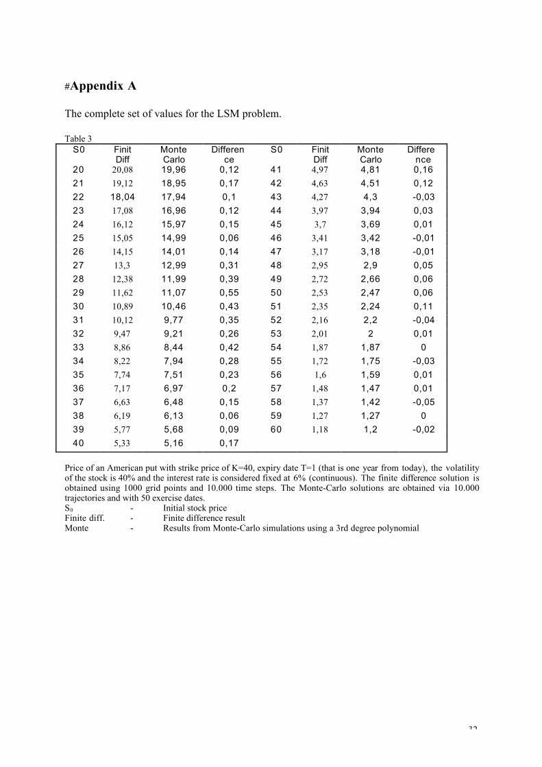
The complete set of values for the LSM problem.

Table 3S0 Finit

DiffMonteCarlo

Difference

S0 FinitDiff

MonteCarlo

Difference

20 20,08 19,96 0,12 41 4,97 4,81 0,16

21 19,12 18,95 0,17 42 4,63 4,51 0,12

22 18,04 17,94 0,1 43 4,27 4,3 -0,03

23 17,08 16,96 0,12 44 3,97 3,94 0,03

24 16,12 15,97 0,15 45 3,7 3,69 0,01

25 15,05 14,99 0,06 46 3,41 3,42 -0,01

26 14,15 14,01 0,14 47 3,17 3,18 -0,01

27 13,3 12,99 0,31 48 2,95 2,9 0,05

28 12,38 11,99 0,39 49 2,72 2,66 0,06

29 11,62 11,07 0,55 50 2,53 2,47 0,06

30 10,89 10,46 0,43 51 2,35 2,24 0,11

31 10,12 9,77 0,35 52 2,16 2,2 -0,04

32 9,47 9,21 0,26 53 2,01 2 0,01

33 8,86 8,44 0,42 54 1,87 1,87 0

34 8,22 7,94 0,28 55 1,72 1,75 -0,03

35 7,74 7,51 0,23 56 1,6 1,59 0,01

36 7,17 6,97 0,2 57 1,48 1,47 0,01

37 6,63 6,48 0,15 58 1,37 1,42 -0,05

38 6,19 6,13 0,06 59 1,27 1,27 0

39 5,77 5,68 0,09 60 1,18 1,2 -0,02

40 5,33 5,16 0,17

Price of an American put with strike price of K=40, expiry date T=1 (that is one year from today), the volatilityof the stock is 40% and the interest rate is considered fixed at 6% (continuous). The finite difference solution isobtained using 1000 grid points and 10.000 time steps. The Monte-Carlo solutions are obtained via 10.000trajectories and with 50 exercise dates.S0 - Initial stock priceFinite diff. - Finite difference resultMonte - Results from Monte-Carlo simulations using a 3rd degree polynomial

33

___________________________________________________________________________

Bibliography___________________________________________________________________________

[1] N.H.Bingham, Rüdiger Kiesel. "Risk-Neutral Valuation", Springer Finance, 1998 [2] B.Djehiche. "Stochastic Calculus, An Introduction with Applications", Kungliga

tekniska högskolan, institutionen för matematik, 2000[3] J.C.Hull. "Options, futures & other derivatives". 4th edition, Prentice Hall, 2000[4] A.Jaun. "Hedging your portfolio: Options, swaps and derivatives",

http://www.lifelong-learners.com/opt[5] A.Jaun. "Numerical methods for partial differential equations",

http://www.lifelong-learners.com/pde[6] F.Longstaff, E.Schwartz. "Interest Rate Volatility and the Term Structure: A Two-

Factor General Equilibrium Model", from The journal of finance, September 1992, vol. 47, 1259-1282.

[7] F.Longstaff, E.Schwartz. "A two-factor interest rate model and contingent claims valuation", from The journal of fixed income, December 1992, vol. 3, 16-23.

[8] F.Longstaff, E.Schwartz. "Implementation of the Longstaff-Schwartz interest rate model", form The journal of fixed income, September 1993, 7-14

[9] F.Longstaff, E.Schwartz. "Comments on "A note on parameter estimation in the two-factor Longstaff and Scwartz model"", from The journal of fixed income, March 1994, 101-102

[10] F.Longstaff, E.Schwartz. "Valuing American Options by Simulation: A Simple Least-Squares Approach", form The review of financial studies, Spring 2001 vol. 14, 113-147

[11] D.G.Luenberger. "Investment science", Oxford university press, 1998[12] R.Rebonato. "Interest-rate option models". 2nd edition, John Wiley and sons, 1998[13] R.Westergren. "Mathematics handbook for science and engineering", studentlitteratur,

1995