Nonlinear Dyn (2021) 103:3489–3513https://doi.org/10.1007/s11071-020-05912-z

ORIGINAL PAPER

Longitudinal–transversal internal resonances inTimoshenko beams with an axial elastic boundary condition

S. Lenci · F. Clementi · L. Kloda ·J. Warminski · G. Rega

Received: 19 April 2020 / Accepted: 20 August 2020 / Published online: 3 September 2020© The Author(s) 2020

Abstract The internal resonances between the longi-tudinal and transversal oscillations of a forced Timo-shenko beam with an axial end spring are studied indepth. In the linear regime, the loci of occurrence of1 : ir , ir ∈ N, internal resonances in the parametersspace are identified. Then, by means of the multipletime scales method, the 1 : 2 case is investigated inthe nonlinear regime, and the frequency response func-tions and backbone curves are obtained analytically,and investigated thoroughly. They are also compared

S. Lenci (B) · F. ClementiDepartment of Civil and Buildings Engineering andArchitecture, Polytechnic University of Marche, ViaBrecce Bianche, 60131 Ancona, Italye-mail: lenci@univpm.it

F. Clementie-mail: francesco.clementi@univpm.it

L. Kloda · J. WarminskiDepartment of Applied Mechanics, Lublin University ofTechnology, Nadbystrzycka 36, 20-618 Lublin, Polande-mail: l.kloda@pollub.pl

J. Warminskie-mail: j.warminski@pollub.pl

G. RegaDepartment of Structural and Geotechnical Engineering,Sapienza University of Rome, Via A. Gramsci 53, 00197Rome, Italye-mail: giuseppe.rega@uniroma1.it

with finite element numerical simulations, to provetheir reliability. Attention is paid to the system responseobtained by varying the stiffness of the end spring,and it is shown that the nonlinear behaviour instanta-neously jumps from hardening to softening by crossingthe exact internal resonance value, in contrast to the sin-gular (i.e. tending to infinity) behaviour of the nonlin-ear correction coefficient previously observed (withoutproperly taking the internal resonance into account).

Keywords Internal resonance · Timoshenko beam ·Multiple time scales method · Nonlinear oscillations ·Hardening/softening

1 Introduction

The dependence of the nonlinear transversal behaviourof beams on different axial boundary conditions isan interesting topic that has been studied by variousauthors. In [1], it was shown that a beam is hardeningif the axial displacement is constrained at the boundaryand is softening if the boundary is free to move axially.These findings were confirmed in [2], where a refinedreduced order model analysis was performed, and theeffect of the axial inertia and inextensibility was inves-tigated.

A fully continuous model was considered in [3],where the multiple time scales method is applieddirectly to the partial differential equations of motion.The results were also compared with some experi-

123

3490 S. Lenci et al.

ments. On the same line of investigation, [4] consideredan axial (i.e. parametric) excitation, and developed theasymptotic analysis up to the fifth order, i.e. one ordermore than what is usually done. Also some experimen-tal results were reported.

In fact, it is known that axial inertia contributesto softening, while the geometrical stiffness, which isstrongly affected by the axial constraint, contributes tohardening. Thewhole behaviour depends onwhich oneof these two opposite phenomena predominates. Thus,it is possible to foresee that introducing at the boundarya spring, of stiffness κ , which allows us to regulate theaxial constraint and thus the geometrical nonlinearity,permits to control the hardening/softening behaviour,passing from softening when κ = 0 (no constraint) tohardening when κ → ∞ (full constraint), that are thelimit cases reported in the earlier literature [1,2].

Although a boundary axial spring is present in [3]and [4], its effect on the softening/hardening behaviouris not fully investigated there. This has been done,instead, in [5], where the dependence of the nonlin-ear correction coefficient ω2 (ω2 > 0 gives hardening,ω2 < 0 provides softening) upon κ is deeply investi-gated. There, also the effects of the axial and rotationalinertia have been studied, as well as those of the shearstiffness and slenderness. A Timoshenko beam modelwas considered to have reliable results also for thickbeams.

Starting from [6], where the equations of motionswere firstly derived and initially analyzed by means ofthe Poincaré–Lindstedt method, and [5], the authorshave done many studies on this topic. In [7], theapproximate analytical results have been comparedwith numerical simulations to check their reliability.In these papers, attention was focused on the transver-sal oscillations, and the axial vibrations are set equalto zero to the first order and appear only to the sec-ond order because of the nonlinear coupling. Actually,this hypothesis has been relaxed in [8], where the axialvibrations to the first order have been considered, too,and the coupling between axial and transversal oscilla-tions is deeply investigated. Interesting, and complex,behaviour charts have been reported, showing that cou-pled and uncoupled solutions can coexist or not, bothbeing hardening or softening.

The difference obtained by considering alternativedefinitions of the curvature (geometric, i.e. dθ

dS , vsmechanical, i.e. dθ

dZ , dS and dZ being the infinitesimal

elements of the deformed and undeformed configura-tions, respectively) in the constitutive behaviour hasbeen the subject of [9] and [10]. It has been shown thatthe difference is of the order of some percents for thickbeams and is totally negligible for slender beams.

While in the previous authors’ work free vibra-tions have been considered, in [11] and [12] the forcedvibrations have been investigated. In [11], the mul-tiple time scales method has been used, and againthe attention was focused on the dependence of thehardening/softening response on the spring stiffness κ .Analytical results have been compared with numerical(FEM) results, showing a good agreement up tomoder-ately largedisplacements, according to the fact that ana-lytical solution is valid only up to the third order. Theappearance of some superharmonic and internal reso-nances has been observed in the numerical simulations.Still in the forced regime, the comparison betweennumerical and experimental resultswas instead the goalof [12], where a very goodmatching has been observed.

The frequency response curves of higher order res-onances have been discussed in [13], where, amongother, it has been stressed that the nonlinear behaviourmay strongly depend on the mode order, for examplethe first mode can be hardening and the second soften-ing.

Within this wide body of research, one aspect hasnot yet been investigated, namely the internal reso-nance between axial and transversal modes. Indeed, in[8] it was assumed that axial and transversal modeswere far away from internal resonance, so that theaxial–transversal coupling was only due to the nonlin-ear effects occurring in kinematically non-condensedstructural models (e.g. [14]). Here, on the contrary, thishypothesis is relaxed, and the internal resonance is fullyinvestigated, both in the linear and nonlinear regimes.In addition to its theoretical and practical effects, thisalso permits to explain a singularity of the nonlinearcorrection coefficient observed in [5] and in [11]. Asdiscussed in more detail in Sect. 2.1 forward, a similarsingular behaviour of the nonlinear correction coeffi-cient, associated with the transition from hardening tosoftening and due to an internal resonance, has beenearlier highlighted in shallow cables [15,16] and inshells [17,18], where only transversal dynamics havebeen studied.

A transition fromhardening to softening, due to 1 : 2internal resonance and not necessarily related to a sin-gular behaviour, has been observed also in a pipe con-

123

Longitudinal–transversal internal resonances in Timoshenko beams 3491

veying fluid [19], where the varying parameter was thefluid velocity, and in a double beam with a tip couplingspring andmagnetic interaction [20], where the drivingparameters were the amplitude of the excitation and thedamping.

Internal resonance, or modal interactions [21], havebeen deeply investigated in the past [22–24], sincethis event can be dangerous (if not properly detected[25]) or useful (if properly exploited, for example inthe field of energy harvesting [26]). However, it seemsthat few attention has been paid to the internal reso-nance between longitudinal and flexural modes. Axial–transversal internal resonances of cables have beeninvestigated, for example, in [27,28], ofmoving belts in[29], while for beams this phenomenon has been inves-tigated in [30], again in the field of axially moving sys-tems. Very few investigations of internal longitudinal–transversal resonance seem to be available for non-moving beams [31].

The paper is organized as follows. The mechanicalmodel is illustrated in Sect. 2, including a summaryof previous results (Sect. 2.1) where the singularity ofthe nonlinear frequency ω2 is highlighted. The occur-rence of various axial–transversal internal resonancesin the slenderness-spring stiffness parameters space isinvestigated in Sect. 3 in the linear regime. Then (Sect.4), attention is focused on 1:2 internal resonance, butnow a nonlinear dynamic analysis is developed withthe multiple time scales method. The main results arereported in Sect. 5, while a comparison of analyticaland numerical outcomes is presented in Sect. 6. Thepaper ends with some conclusions and suggestions forfurther developments (Sect. 7).

2 The mathematical model

We consider the Timoshenko beam illustrated in Fig. 1.Its rest configuration is rectilinear, along the Z direc-tion, it is made of a linearly elastic and homogeneousmaterial, and its cross section is constant. W (Z , T ),U (Z , T ) and θ(Z , T ) are the axial and transversal dis-placements of the beam axis, and the rotation of thecross section. Z is the spatial coordinate in the refer-ence (straight) configuration, measuring the physicaldistance from the left boundary, and T is the time.

The axial, shear and bending stiffnesses are E A,GAand E J , respectively. The axial and transversal massper unit length is ρA, while the rotational inertia is ρ J .

Fig. 1 Timoshenko beam with axial end spring

κ is the stiffness of the linear spring at the right-endof the beam (Fig. 1), which acts in the Z (axial) direc-tion. CW , CU and Cθ are the (linear) damping coef-ficients along the respective directions. The beam isexcited by a dead load PU (Z , T ) = F(Z , T ) acting inthe X direction, which is perpendicular to Z . Introduc-ing axial, PW (Z , T ), and rotational, Pθ (Z , T ), loads isconceptually easy but will not be pursued to limit thecomputational efforts.

The kinematically exact equations of motion havebeen derived in [6] (see also [5,8,11]) and are givenby:

{E A[

√(1 + W ′)2 +U ′2 − 1] 1 + W ′√

(1 + W ′)2 +U ′2

+GA

[θ − arctan

(U ′

1 + W ′

)]U ′√

(1 + W ′)2 +U ′2

}′

= ρA W + CW W ,{E A[

√(1 + W ′)2 +U ′2 − 1] U ′√

(1 + W ′)2 +U ′2

−GA

[θ − arctan

(U ′

1 + W ′

)]1 + W ′√

(1 + W ′)2 +U ′2

}′

= ρA U + CUU + F(Z , T ),[E J

θ ′√(1 + W ′)2 +U ′2

]′

− GA

[θ − arctan

(U ′

1 + W ′

)] √(1 + W ′)2 +U ′2

= ρ J θ + Cθ θ , (1)

where the prime denotes derivative with respect to Zand dot derivative with respect to T .

The boundary conditions in the transversal directionare:

U (0, T ) = 0, M(0, T ) = 0,

U (L , T ) = 0, M(L , T ) = 0, (2)

123

3492 S. Lenci et al.

where M is the bending moment,

M = E Jdθ

dS= E J

dθ

dZ

dZ

dS

= E Jθ ′

S′ = E Jθ ′√

(1 + W ′)2 +U ′2 , (3)

i.e. the geometrical curvature is considered. A possiblealternative is to use themechanical curvature, assumingM = E J dθ

dZ [9,10].The boundary conditions in the axial direction are:

W (0, T ) = 0, Ho(L , T ) + κW (L , T ) = 0, (4)

where Ho(Z , T ) is the internal horizontal force in theZ direction and is given by

Ho = E A

√(1 + W ′)2 +U ′2 − 1√

(1 + W ′)2 +U ′2 (1 + W ′)

+GAθ − arctan

(U ′

1+W ′)

√(1 + W ′)2 +U ′2U

′. (5)

2.1 Previous results

By applying the Poincaré–Lindstedt method (in [5,6])and the multiple time scales method (in [11]), and byconsidering only the transversal displacements up tothe first order, the following approximate solution waspreviously obtained for the free oscillations:

W (Z , T ) = 0 + · · · ,

U (Z , T ) = Ua sin

(n π Z

L

)sin(ω f T ) + · · · ,

θ(Z , T ) = Ua

L

(n π − ω2

0

n π z l2

)

× cos

(n π Z

L

)sin

(ω f T

) + · · · , (6)

where Ua is the amplitude of the transversal motion,n ∈ N the mode number, and where, most importantly,

ω f = ω f 0 +(Ua

L

)2

ω f 2 + · · ·

= 1

L2

√E J

ρA

[ω0 +

(Ua

L

)2

ω2 + · · ·]

(7)

is the nonlinear frequency of the free motion.In (7), ω0 is the dimensionless natural (linear) fre-

quencyof the transversalmotion,whileω2 is the dimen-sionless nonlinear correction coefficient, also known as“nonlinear frequency correction”, whichmeasures howthe nonlinear frequency is affected by the amplitudeof the motion. It was the most important result, sinceit summarizes the nonlinear behaviour of the system:hardening for ω2 > 0, softening for ω2 < 0.

For the boundary conditions (2), it is possible tocompute

ω0 = l

2

√zl2 + n2π2(1 + z) −

√z2l4 + 2zn2π2(1 + z)l2 + n4π4(1 − z)2, (8)

where n ∈ N is the order of the transversal (flexural)natural frequency and the following three dimension-less parameters are introduced:

l = L

√E A

E J, z = GA

E A= 1

2(1 + ν)χ, κh = L3

E Jκ,

(9)

(l is the slenderness of the beam, ν the Poisson coeffi-cient and χ the shear correction factor) so that

E A = E J

L2 l2, ρ J = ρA L2

l2, GA = E J

L2 l2z. (10)

κh is the dimensionless stiffness of the axial spring atZ = L , that will be used in the rest of the paper. Weconsider ν = 0.3 and χ = 1.17, namely z = 0.3287,so that the unique parameters are l and κh, together withthe order n of the natural frequency.

For the sameboundary conditions, the nonlinear cor-rection coefficient is

ω2 = c1ω2a + c2 sin (2ω0/ l) ω2b + ω2c

ω2d, (11)

where the parameters appearing in (11) are reported in“Appendix”.

For κh = 50 and n = 1, the function ω2(l) is plottedin Fig. 2, which corresponds to Fig. 10b of [5].

123

Longitudinal–transversal internal resonances in Timoshenko beams 3493

Fig. 2 The function ω2(l) for κh = 50 and n = 1

For the scope of the present work, the most relevantproperty of Fig. 2 is that ω2(l) has a singular point forlsing = 8.149112. It has also a zero point at lzero =11.379729. When crossing these points, the sign of ω2

changes, and, for increasing l, we pass from hardeningto softening and again to hardening.

The singular and zero points are not specific of theconsidered value of κh, but they persist, as shown inFig. 3, corresponding to Fig. 12c of [5].

In [5], eq. (27), looking at the expressions of ω2, itwas noted that the singular points occur when

κh = −2 l ω0cos (2ω0/ l)

sin (2ω0/ l), (12)

namely when the denominator of c2 is zero. This phe-nomenon was also observed in [11], and in [32] itis mentioned that it is due to an internal resonancebetween axial and transversal modes. Confirming thisproperty in the considered mechanical system, andstudying in depth the internal resonances, is the maingoal of this paper.

Before to proceed, we note that the singular pointsin Fig. 3 occur for quite low values of the slenderness(thick beams, but still compatible with the Timoshenkobeam theory). Actually, for n = 2 the singular pointshappen for larger values of l (in the realm of slenderbeams), as shown by the example of Fig. 4, which cor-responds to Fig. 3 of [11] (but note that a different

Fig. 3 The zero (continuous line) and singular (dash line) valuesof ω2 for n = 1. The dots are the points corresponding to Fig. 2,where κh = 50

Fig. 4 The function ω2(κh) for l = 10√12 = 34.6410 and

n = 2

rescaling of the spring stiffness is used there) and toa beam with square cross section and length equal to10 times the thickness. Here, κh,sing = 1661.24 andκh,zero = 2122.32.

For n = 2, the zero and singular points are reportedin Fig. 5. Note that in this parameters window there aretwo singularities and zeros. The lowest zero and sin-

123

3494 S. Lenci et al.

Fig. 5 The zero (continuous lines) and singular (dash lines) val-ues of ω2 for n = 2. The dots are the points corresponding toFig. 4, where l = 10

√12 = 34.6410

gular curves almost coincide. If one would enlarge theview, more singular and zero branches would appear.

Although the motivation of the present paper comesmainly from the authors’ previous work summa-rized above, it is worth mentioning that the singularbehaviour of the nonlinear correction coefficient in cor-respondence of internal resonances, and in particular1 : 2 internal resonance, has been previously observedfor different mechanical systems in the framework ofthe reduction methods evaluation.

In [15], the singularity has been reported for the firstin-plane (vertical) mode of a suspended cable. Here,the varying parameter is an elasto-geometric parametertaking into account stiffness and sag-to-span ratio, andthe singularity is due to the breakdown ofmodal expan-sions not explicitly considering the internal resonance.For the same structure, a similar, but deeper, analysishas been reported in [16], where also the out-of-planebehaviour has been considered. Here, it is shown thatdiscretized approaches, where the Galerkin reductionmethod is applied before theMTS, fail to detect the sin-gular behaviour if a sufficiently large number of modesis not considered.

Using nonlinear normal modes to highlight harden-ing/softening behaviour of nonlinear systems [33], thesingular behaviour of the nonlinear correction coeffi-cient for a free-edge shallow spherical shell has been

shown in [17], where the driving parameter is the aspectratio, which is governed by the geometrical propertiesof the system. Within a study of the effect of the num-ber of retained modes in a Galerkin reduction, manycurves similar to Figs. 2 and 4 have been reported. Itis remarked that only 1 : 2 internal resonance of cer-tain modes are able to generate the singular behaviour,while other modes and other resonances (e.g. 1 : 3)do not have this effect. In [18], it has been shownthat the addition of damping will smooth the singularbehaviour, while keeping the large (but finite) valuesof ω2 for small values of damping.

In the previous papers, the singular behaviour, andthe 1 : 2 internal resonance lurking in the background,have been reported. However, a detailed asymptoticexpansion considering the internal resonance is not car-ried out. This analysis has been done in [19,20], where,however, no singular behaviour is observed in the back-ground. In the present work, we complete, and some-how connect, the two groups of works, while referringto the longitudinal–transverse coupling in the mechan-ical system of our interest.

3 Longitudinal–transversal internal resonance:linear analysis

The occurrence of the longitudinal–transversal internalresonance in the parameters space (κh,l) can be detectedin the linear regime, where the two modal problemsare independent from each other (since the beam isrectilinear). This constitutes the aim of this section. Thenonlinear coupling in the neighbourhood of internalresonances will be investigated in the next section.

The transversal natural frequency ω f 0 is given (indimensionless form) by (8). The axial natural frequencyωa0, the solution of

E Aw′′(Z) + ω2a0 ρAw(Z) = 0,

w(0) = 0, E Aw′(L) + κ w(L) = 0, (13)

can be easily computed by standard methods (see alsoSect. 4.1) and is given by

ωa0 = x

L

√E A

ρA= x l

L2

√E J

ρA, (14)

x being the solution of

123

Longitudinal–transversal internal resonances in Timoshenko beams 3495

x l2 cos(x) + sin(x)κh = 0. (15)

The associated mode shape is w(Z) = sin(x Z/L).Note that for very small values of κh/ l2 the solutions of(15) are xm ∼= π/2+(m−1)π ,m ∈ Nbeing the order ofthe axial natural frequency, while for very large valuesof κh/ l2 the solutions of (15) are xm ∼= mπ . Thus,for varying κh/ l2 ∈ [0,∞[ the following bounds hold:π/2 + (m − 1)π ≤ xm ≤ mπ .

The expression (15) can be rewritten as

κh = −l2 xcos(x)

sin(x). (16)

When x = 2ω0/ l, namely when ωa0 = 2ω f 0, equa-tion (16) is identical to (12), and this clearly shows thatthe singular points of ω2 are due to the 1 : 2 internalresonance between transversal and axial modes.

Reasoning in a similar fashion, it is not difficult toforesee that singular points of ω4 (the next term in thedevelopment (7)) will be due to a 1:4 internal resonancebetween transversal and axial modes and so on. Thisaspect will not be pursued here and is left for futureworks.

To generalize the previous considerations, we inves-tigate the 1 : ir internal resonances, those such thatωa0

ω f 0= ir, ir ∈ N. (17)

The study of other internal resonances, for example2ωa0 = ω f 0, is left for future works.

Combining (7), (8), (14), (16) and (17), it is easy toobtain

κh,ir (l) = −l ir ω0cos(ir ω0/ l)

sin(ir ω0/ l). (18)

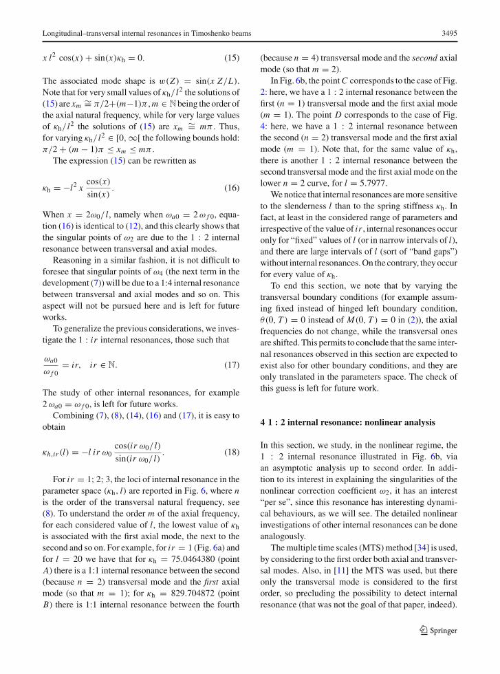
For ir = 1; 2; 3, the loci of internal resonance in theparameter space (κh, l) are reported in Fig. 6, where nis the order of the transversal natural frequency, see(8). To understand the order m of the axial frequency,for each considered value of l, the lowest value of κhis associated with the first axial mode, the next to thesecond and so on. For example, for ir = 1 (Fig. 6a) andfor l = 20 we have that for κh = 75.0464380 (pointA) there is a 1:1 internal resonance between the second(because n = 2) transversal mode and the first axialmode (so that m = 1); for κh = 829.704872 (pointB) there is 1:1 internal resonance between the fourth

(because n = 4) transversal mode and the second axialmode (so that m = 2).

In Fig. 6b, the pointC corresponds to the case of Fig.2: here, we have a 1 : 2 internal resonance between thefirst (n = 1) transversal mode and the first axial mode(m = 1). The point D corresponds to the case of Fig.4: here, we have a 1 : 2 internal resonance betweenthe second (n = 2) transversal mode and the first axialmode (m = 1). Note that, for the same value of κh,there is another 1 : 2 internal resonance between thesecond transversal mode and the first axial mode on thelower n = 2 curve, for l = 5.7977.

Wenotice that internal resonances aremore sensitiveto the slenderness l than to the spring stiffness κh. Infact, at least in the considered range of parameters andirrespective of the value of ir , internal resonances occuronly for “fixed” values of l (or in narrow intervals of l),and there are large intervals of l (sort of “band gaps”)without internal resonances.On the contrary, theyoccurfor every value of κh.

To end this section, we note that by varying thetransversal boundary conditions (for example assum-ing fixed instead of hinged left boundary condition,θ(0, T ) = 0 instead of M(0, T ) = 0 in (2)), the axialfrequencies do not change, while the transversal onesare shifted. This permits to conclude that the same inter-nal resonances observed in this section are expected toexist also for other boundary conditions, and they areonly translated in the parameters space. The check ofthis guess is left for future work.

4 1 : 2 internal resonance: nonlinear analysis

In this section, we study, in the nonlinear regime, the1 : 2 internal resonance illustrated in Fig. 6b, viaan asymptotic analysis up to second order. In addi-tion to its interest in explaining the singularities of thenonlinear correction coefficient ω2, it has an interest“per se”, since this resonance has interesting dynami-cal behaviours, as we will see. The detailed nonlinearinvestigations of other internal resonances can be doneanalogously.

Themultiple time scales (MTS)method [34] is used,by considering to the first order both axial and transver-sal modes. Also, in [11] the MTS was used, but thereonly the transversal mode is considered to the firstorder, so precluding the possibility to detect internalresonance (that was not the goal of that paper, indeed).

123

3496 S. Lenci et al.

(a) (b)

(c) (d)

Fig. 6 The loci of internal resonance. a ir = 1 (i.e. ω f 0 : ωa0 = 1 : 1), b ir = 2 (i.e. ω f 0 : ωa0 = 1 : 2), c and d ir = 3 (i.e.ω f 0 : ωa0 = 1 : 3). n is the order of the transversal frequency. (Color figure online)

Axial and transversal modes to the first order are alsoconsidered in [8], but there it is implicity assumed thatthey are not in internal resonance, since the aim wasto detect the axial–transversal nonlinear coupling in ageneral fashion, and not only around specific values ofthe parameters where internal resonance occurs.

With the MTS method, the solution is sought afterin the asymptotic form

W (Z , T ) = εW1(Z , T0, T1) + ε2W2(Z , T0, T1) + · · · ,

U (Z , T ) = εU1(Z , T0, T1) + ε2U2(Z , T0, T1) + · · · ,

θ(Z , T ) = εθ1(Z , T0, T1) + ε2θ2(Z , T0, T1) + · · · , (19)

where ε is a bookeeping small parameter introducedto stress that we are studying moderate displacementsand rotation around the rest position. T0 = T is thephysical (fast) time, and Ti = εi T , i ≥ 1 are the slowtimes.

123

Longitudinal–transversal internal resonances in Timoshenko beams 3497

It is further assumed that the excitation is harmonicin time (with frequency ), and that damping and loadscale according to

CW = εcW , CU = εcU ,

Cθ = εcθ , F(Z , T ) = ε2 f (Z) cos(T ). (20)

Inserting the expressions (19)–(20) in the asymp-totic expansion of the governing equations (1), andequating to zero the coefficients of εi , a sequence oflinear problems is derived. They are investigated in thenext subsections.

4.1 First-order problem

The first-order equations read

E AW ′′1 − ρA

∂2W1

∂T 20

= 0,

GA(θ ′1 −U ′′

1 ) + ρA∂2U1

∂T 20

= 0,

E J θ ′′1 − GA(θ1 −U ′

1) − ρ J∂2θ1

∂T 20

= 0, (21)

and the related boundary conditions are (the depen-dence on time is omitted for simplicity)

W1(0) = 0, E AW ′1(L) + κ W1(L) = 0,

U1(0) = 0, θ ′1(0) = 0,

U1(L) = 0, θ ′1(L) = 0. (22)

The solution of (21), (22) is given by (the over barstands for complex conjugate and I is the imaginaryunit)

W1(Z , T0, T1) = W1a(Z)[B(T1)eIωa0T0

+ B(T1)e−Iωa0T0 ],

U1(Z , T0, T1) = U1a(Z)[A(T1)eIω f 0T0

+ A(T1)e−Iω f 0T0 ],

θ1(Z , T0, T1) = θ1a(Z)[A(T1)eIω f 0T0+

+ A(T1)e−Iω f 0T0 ], (23)

where the functions W1a(Z), U1a(Z) and θ1a(Z) arereported in “Appendix”, and A(T1) and B(T1) are com-plex amplitudes of the transversal and axial oscilla-tions, respectively. ωa0 is given by (14) (with x given

by (15)), while ω f 0 is given by (7) with ω0 given by(8).

Note that in [5–7,9,11], but not in [8], itwas assumedW1a(Z) = 0.

4.2 Second-order problem

The second-order equations read

E AW ′′2 − ρA

∂2W2

∂T 20

= cW∂W1

∂T0+ 2 ρA

∂2W1

∂T0T1

−[(E A/2 − GA)U ′2

1 + GAU ′1θ1

]′,

GA(θ ′2 −U ′′

2

) + ρA∂2U2

∂T 20

= −cU∂U1

∂T0− 2 ρA

∂2U1

∂T0T1+ f (Z) cos(T0) + (E A − GA)(U ′

1W′1)

′,

E J θ ′′2 − GA(θ2 −U ′

2) − ρ J∂2θ2

∂T 20

= cθ

∂θ1

∂T0

+ 2 ρ J∂2θ1

∂T0T1+ GAW ′

1θ1 + E J (W ′1θ

′1)

′, (24)

and the related boundary conditions are (the depen-dence on time is omitted for simplicity)

W2(0) = 0, E AW ′2(L) + κ W2(L)

= −(E A/2 − GA)U ′21 (L) − GAU ′

1(L)θ1(L),

U2(0) = 0, θ ′2(0) = 0,

U2(L) = 0, θ ′2(L) = 0. (25)

It is now necessary to introduce the 1 : 2 internalresonance condition,

ωa0 = 2ω f 0 + εσi → ωa0T0 = 2ω f 0T0 + σi T1, (26)

together with the external resonance,

= ω f 0 + εσe → T0 = ω f 0T0 + σeT1, (27)

123

3498 S. Lenci et al.

where σi and σe are the detuning parameters measuringthe distance (in the frequency) from the perfect internaland external resonances, respectively. Note that, com-bining (26) and (27), we have

2 = ωa0 + ε(2σe − σi ), (28)

so that the detuning between 2 and ωa0 is given by(2σe − σi ).

The particular solution of (24) is given by

W2(Z , T0, T1) = W2a(Z , T1)eIωa0T0

+ W2a(Z , T1)e−Iωa0T0

+ W2b(Z , T1),

U2(Z , T0, T1) = U2a(Z , T1)eIω f 0T0

+ U2a(Z , T1)e−Iω f 0T0

+U2b(Z , T1)e3Iω f 0T0

+ U2b(Z , T1)e−3Iω f 0T0 ,

θ2(Z , T0, T1) = θ2a(Z , T1)eIω f 0T0

+ θ2a(Z , T1)e−Iω f 0T0

+ θ2b(Z , T1)e3Iω f 0T0

+ θ2b(Z , T1)e−3Iω f 0T0 . (29)

It is worth to note that the homogenous solution of (24),that adds to (29), is not needed in this work.

Inserting (29) in (24), and in the boundary condi-tions, we obtain the following problems for W2a(Z),U2a(Z) and θ2a(Z):

E AW ′′2a + ω2

a0 ρAW2a

= − f ′We−Iσi T1 A(T1)

2

+ Iωa0W1a

[2ρA

dB

dT1(T1) + cW B(T1)

],

W2a(0) = 0, E AW ′2a(L) + κW2a(L)

= − fW (L)e−Iσi T1 A(T1)2,

− GA(U ′2a − θ2a)

′ − ω2f 0 ρAU2a

= − f ′Ue

Iσi T1 A(T1)B(T1)

− Iω f 0U1a

[2 ρA

dA

dT1(T1) + cU A(T1)

]+ f (Z)

2eIσeT1 ,

E Jθ ′′2a + GA

(U ′2a − θ2a

)+ ω2

f 0 ρ J θ2a

= [ f ′θ + GAW ′

1a θ1a)]eIσi T1 A(T1)B(T1)

+ Iω f 0 θ1a

[2 ρ J

dA

dT1(T1) + cθ A(T1)

],

U2a(0) = U2a(L) = θ ′2a(0) = θ ′

2a(L) = 0, (30)

where the functions fW , fU and fθ are reported in“Appendix”.

4.3 Frequency response curves

The solvability conditions for the second-order prob-lems (30) are

Iωa0

[2 ρA r1

dB

dT1(T1) + cW r1B(T1)

]+ r2 e

−Iσi T1 A(T1)2 = 0,

Iω f 0

[2 (ρA r3 + ρ J r4)

dA

dT1(T1)

+ (cU r3 + cθ r4) A(T1)

]+ r5 e

Iσi T1 A(T1)B(T1) = r6eIσeT1 , (31)

where theparameters r1, . . . , r6 are reported in “Appendix”.Note that the load is accounted for in r6. Rememberingthat x = x(κh, l,m), we observe that the other coeffi-cients depend on l, κh, z (that is kept fixed in this work)and the order of transversal (n) and axial (m) naturalfrequencies.

As customary [34], the solution of (31) is soughtafter in the polar form

A(T1) = a(T1)

2e−I [σeT1+βa(T1)],

B(T1) = b(T1)

2e−I [(2σe−σi )T1+βb(T1)], (32)

where a(T1) and b(T1) are real value amplitudes of thetransversal and axial (first order) motions, respectively,and βa(T1) and βb(T1) are real value phase differences.In fact, rearranging (23) we obtain

W1 = b(T1) cos[2T + βb(T1)]W1a(Z),

U1 = a(T1) cos[T + βa(T1)]U1a(Z),

θ1 = a(T1) cos[T + βa(T1)]θ1a(Z). (33)

Inserting (32) in (31) and separating real from imag-inary parts, we obtain, after some algebra,

123

Longitudinal–transversal internal resonances in Timoshenko beams 3499

da

dT1= −1

2

cU r3 + cθ r4ρA r3 + ρ J r4

a

+ r5 sin (2βa − βb)

4ω f 0(ρA r3 + ρ J r4)a b

− sin(βa)

ω f 0(ρA r3 + ρ J r4)r6,

dβa

dT1= −σe + r5 cos(2βa − βb)

4ω f 0 (ρA r3 + ρ J r4)b

− cos(βa)

ω f 0 (ρA r3 + ρ J r4)

r6a

,

db

dT1= −1

2

cWρA

b − r2 sin (2βa − βb)

4ωa0 ρA r1a2,

dβb

dT1= −2σe + σi + r2 cos (2βa − βb)

4ωa0 ρA r1

a2

b. (34)

that are commonly known as modulation equations.Here, the dependence on T1 is omitted for brevity.

Because of (33), steady oscillations of the beam cor-respond to equilibrium points of (34). Setting equal tozero the derivatives in (34), we obtain an algebraic sys-tem in the four unknowns a, b, βa and βb, that are nowconstant.

From the third and fourth equations, we obtain

b = r2

2ωa0r1√4(2 σe − σi )2(ρA)2 + c2W

a2,

tan (2 βa − βb) = − cW2(2σe − σi )ρA

. (35)

Using (35) in the first and second equations of (34),we obtain

tan(βa) =4(cU r3 + cθ r4)ω f 0 + r2 r5cW

ωa0r1[4(2 σe−σi )

2(ρA)2+c2W]a2

8 (ρA r3 + ρ J r4) σeω f 0 − 2 r2 r5ρAωa0r1

[4(2 σe−σi )

2(ρA)2+c2W]a2 .

(36)

and the equation

r22 r25

64 r21ω2a0

[4(2 σe − σi )2(ρA)2 + c2W

]a6− r2 r5 ω f 0 [4ρA σe (2σe − σi ) (ρA r3 + ρ J r4) − cW (cU r3 + cθ r4)]

8 r1ωa0[4(2 σe − σi )2(ρA)2 + c2W ] a4

+ ω2f 0

[4 σ 2

e (ρA r3 + ρ J r4)2 + (cU r3 + cθ r4)2]

4a2 = r26 , (37)

which is third order in the unknown y = a2,so that its closed form solution is known. Oncea(l, κh, n,m, cW , cU , cθ , r6,) has been determined,b,βa andβb can be computed from (35) and (36).Whenall parameters are fixed, and only the external excitation is varied, the searched frequency response curves(FRCs) are obtained.

Equation (37) is cubic in a2. Thus, there alwaysexists a real solution. Furthermore, it may happen thatthree real solutions exist. This occurs in particular inthe neighbourhood of resonance, as we will see in thefollowing.

In the very special case of perfect internal (σi = 0)and external (σe = 0) resonances, i.e. ωa0 = 2ω f 0 =2, Eq. (37) reduces to

a

∣∣∣∣ 116 r2 r5 a2

r1cWω f 0+ 1

2ω f 0(cU r3 + cθr4)

∣∣∣∣ = |r6|. (38)

In this case, the asymptotic development of the solutionwith respect to cW is given by

a = 3

√16 r1 r6 ω f 0

r2 r53√cW + · · · ,

b = 3

√4 r2 r26

r1 r25 ω f 0

1

cW+ · · · , (39)

which shows that for cW → 0 we have b → ∞. Thishighlights the role played by cW in the resonance.

The stability of the solutions previously obtainedcan be determined by computing the eigenvalues of theJacobian of the right-hand side of (34) at each equilib-rium point. If all the four eigenvalues have negative realpart, the solution is stable; otherwise, it is unstable. Inparticular, if there is a real positive eigenvalue, the solu-tion is a saddle, while if there is a complex eigenvaluewith positive real part, the solution is a source.

123

3500 S. Lenci et al.

By varying the parameters, if a real eigenvaluepasses from negative to positive, we have a saddle–node bifurcation, while if a complex eigenvalue passesfrom negative real part to positive, we have a Neimark–Sacker, or secondary Hopf, bifurcation, and a quasi-periodic solution is born in the mechanical system.Because of their geometrical properties, saddle–nodebifurcations can be detected by looking for the zeros ofthe discriminant of Eq. (37), where we pass from 1 to3 real solutions.

4.4 Backbone curves

In the absence of excitation, r6 = 0, and damping,cW = cU = cθ = 0, the beam undergoes a freemotion,of frequency (see 33). In this case, (37) simplifies to

r22 r25

256 r21ω2a0 (2 σe − σi )

2 (ρA)2a6

− r2 r5 ω f 0 σe (ρA r3 + ρ J r4)

8 r1ωa0(2 σe − σi )ρAa4

+ ω2f 0 σ 2

e (ρA r3 + ρ J r4)2a2 = 0, (40)

which can be rewritten as

a2(

r2 r516 r1 ωa0 (2 σe − σi ) ρA

a2

−ω f 0 σe (ρA r3 + ρ J r4))2 = 0. (41)

Thus, excluding the trivial solution a = 0, we have

a2 = 16r1 ρA (ρA r3 + ρ Jr4)

r2 r5ωa0 ω f 0σe (2 σe − σi ) ,

(42)

and then (the sign function is sign(y) = y/|y|)

b = 4ρA r3 + ρ J r4

r5ω f 0 σe sign (2 σe − σi ) . (43)

They represent the analytical expressions for the so-called BackBone Curves (BBCs) of coupled oscilla-tors, which give the amplitudes of the oscillation as afunction of the vibration frequency . As it happensfor the BBCs of uncoupled oscillators [34], they arealso the loci of maximum points of frequency responsecurves, as we will see in the next section.

When all parameters but are fixed, only σe is vary-ing in (42) and (43), so that a(σe) ∼ √

σe(2 σe − σi )

and b(σe) ∼ σe sign(2 σe − σi ), this being a prop-erty that helps to understand the behaviour of theBBCs. In particular, we note that a(σe) exists onlywhen σe /∈ [min{0, σi/2};max{0, σi/2}], and locallyit behaves like a square root. b(σe) exists in the samerange, where it is (piecewise) linear.

In the very special case of perfect resonance, σi = 0and ωa0 = 2ω f 0, the previous expressions simplify to

a = 8

√r1 ρA (ρA r3 + ρ Jr4)

r2 r5ω f 0 |σe|,

b = 8(ρA r3 + ρ J r4)

r5ω f 0|σe|, (44)

and both curves become proportional to |σe| (see forth-coming Fig. 9d).

5 Results

Although the analysis of the solution can be done indimensionless form, to refer to a real case and to com-pare the results with those obtained by numerical sim-ulations, we prefer to deal with a dimensional case.

We choose a beam of 0.05 × 0.05 m2 square crosssection,made of steel (E = 2.1×1011 N/m2,ρ = 7850kg/m3, ν = 0.3), of length L = 0.5 m. We then havel = 10

√2 = 34.6410 and z = 0.3287, so that we

are exactly in the case of Fig. 4. We also have ω f 0 =11089.77 rad/s (the period is 5.66 × 10−4 sec) andωa0 = 10344.39 x rad/s. For this case, the perfect 1 :2 internal resonance between the second transversalmode (n = 2) and the first axial mode (m = 1) isobtained at κh,ir = 1661.24, see point “D” in Fig. 6b.We will vary κh around this value.

We further assume CW = CU = 50 N sec/m2 andCθ = 1.5 N sec. The load is a concentrated force Qapplied at L/4 (in order to excite the second transversalmode), so that r6 = Q sin(n π/4)/2 = Q/2 N (sincen = 2). Any other distribution of load providing thesame r6 is equivalent to the present one. For comparisonwith the forthcoming dynamical case, we note that thetransversal static displacement in the point where theforce is applied is,within the small displacements lineartheory, U (L/4) = (3/256)(Q L3/E J ) = 0.0134 mmfor Q = 1000 N.

123

Longitudinal–transversal internal resonances in Timoshenko beams 3501

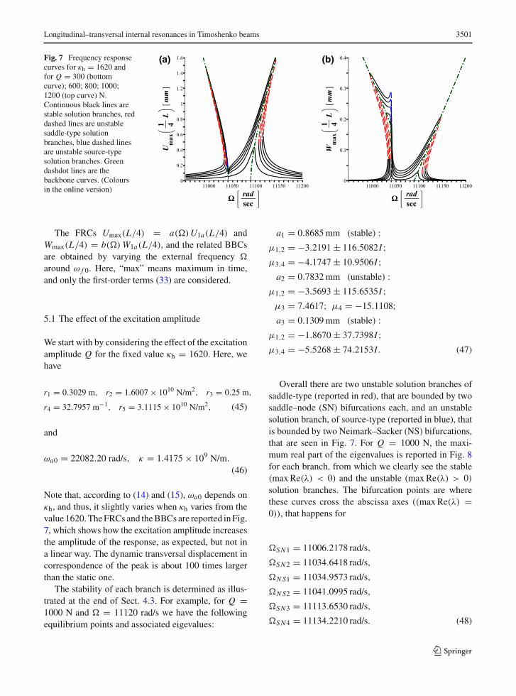
Fig. 7 Frequency responsecurves for κh = 1620 andfor Q = 300 (bottomcurve); 600; 800; 1000;1200 (top curve) N.Continuous black lines arestable solution branches, reddashed lines are unstablesaddle-type solutionbranches, blue dashed linesare unstable source-typesolution branches. Greendashdot lines are thebackbone curves. (Coloursin the online version)

(a) (b)

The FRCs Umax(L/4) = a()U1a(L/4) andWmax(L/4) = b()W1a(L/4), and the related BBCsare obtained by varying the external frequency

around ω f 0. Here, “max” means maximum in time,and only the first-order terms (33) are considered.

5.1 The effect of the excitation amplitude

We start with by considering the effect of the excitationamplitude Q for the fixed value κh = 1620. Here, wehave

r1 = 0.3029 m, r2 = 1.6007 × 1010 N/m2, r3 = 0.25 m,

r4 = 32.7957 m−1, r5 = 3.1115 × 1010 N/m2, (45)

and

ωa0 = 22082.20 rad/s, κ = 1.4175 × 109 N/m.

(46)

Note that, according to (14) and (15), ωa0 depends onκh, and thus, it slightly varies when κh varies from thevalue 1620.TheFRCs and theBBCsare reported inFig.7, which shows how the excitation amplitude increasesthe amplitude of the response, as expected, but not ina linear way. The dynamic transversal displacement incorrespondence of the peak is about 100 times largerthan the static one.

The stability of each branch is determined as illus-trated at the end of Sect. 4.3. For example, for Q =1000 N and = 11120 rad/s we have the followingequilibrium points and associated eigevalues:

a1 = 0.8685mm (stable) :μ1,2 = −3.2191 ± 116.5082I ;μ3,4 = −4.1747 ± 10.9506I ;a2 = 0.7832mm (unstable) :

μ1,2 = −3.5693 ± 115.6535I ;μ3 = 7.4617; μ4 = −15.1108;a3 = 0.1309mm (stable) :

μ1,2 = −1.8670 ± 37.7398I ;μ3,4 = −5.5268 ± 74.2153I. (47)

Overall there are two unstable solution branches ofsaddle-type (reported in red), that are bounded by twosaddle–node (SN) bifurcations each, and an unstablesolution branch, of source-type (reported in blue), thatis bounded by two Neimark–Sacker (NS) bifurcations,that are seen in Fig. 7. For Q = 1000 N, the maxi-mum real part of the eigenvalues is reported in Fig. 8for each branch, from which we clearly see the stable(maxRe(λ) < 0) and the unstable (maxRe(λ) > 0)solution branches. The bifurcation points are wherethese curves cross the abscissa axes ((maxRe(λ) =0)), that happens for

SN1 = 11006.2178 rad/s,

SN2 = 11034.6418 rad/s,

NS1 = 11034.9573 rad/s,

NS2 = 11041.0995 rad/s,

SN3 = 11113.6530 rad/s,

SN4 = 11134.2210 rad/s. (48)

123

3502 S. Lenci et al.

Fig. 8 The maximum real part of the eigenvalues for κh = 1620and Q = 1000 N. Continuous black lines are stable solutionbranches, red dashed lines are unstable saddle-type solutionbranches, blue dashed lines are unstable source-type solutionbranches. (Colours in the online version)

The source-type unstable solution branch is quite nar-row. For low values of the load (Q = 300 N), there isa unique stable solution branch, having peaks in corre-spondence of the resonances.

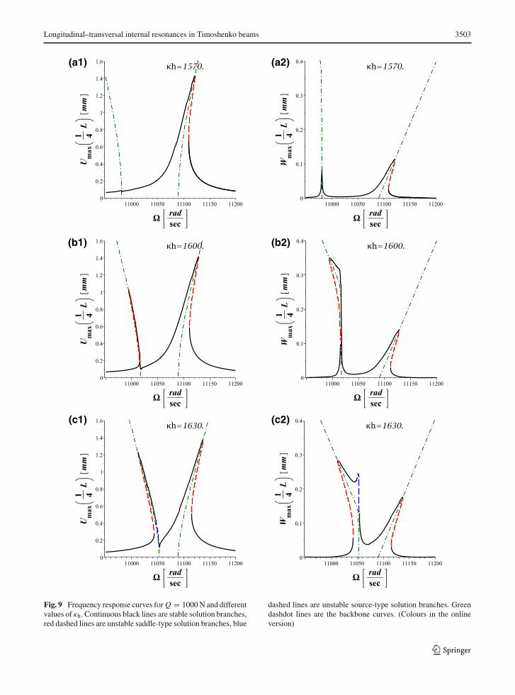
5.2 The transition from hardening to softening

The transition from hardening to softening is illus-trated in Fig. 9 to show what really happens throughthe (apparent) singularity of Fig. 4. For κh quite belowκh,ir (Fig. 9a),we are far from the internal resonance. Incorrespondence of ωa0/2, there is no amplification onU , because the excitation is not in primary resonancewith the transversal mode, while we have a classicalresonance curve in W , which is practically vertical.Here, the resonance mechanism is the following: (1)the external excitation induces small vibration on thetransversal displacement; (2) the weak nonlinear cou-pling from U to W , illustrated in [8], induces smalloscillations on the axial displacement; (3) since theexternal excitation is just in order-2 superharmonic res-onance with the axial mode, there is a resonance ampli-fication, linear because the transversal mode transfersonly a small amount of energy to the axial one. In turn,around ω f 0, the FRC of U is hardening (in agreement

with ω2 > 0 in Fig. 4), and that of W behaves simi-larly, due again to the mere nonlinear coupling awayfrom internal resonance [8]. Note that the transversaldisplacement (directly excited) is about 15 times largerthan the axial one.

Increasing κh (Fig. 9b), the major change is that asoftening resonance curve is observed in bothW andUaround ωa0/2. The meaningful nonlinear effect of theinternal resonance is apparent in the left peaks, the Wone beingmuchmore important than the correspondinghardening peak aroundω f 0 which represents the nearlyunchanged effect from U to W due to the nonlinearcoupling. Note also the clearly visible piecewise linearbehaviour of the BBCs of b in Fig. 9b2.

By further increasing κh (Fig. 9c), thus getting closerto the exact internal resonance, the softening FRCaround ωa0/2 becomes more important, both in termsof U and W . In W , a third peak appears exactly atωa0/2, suggesting a further second-order coupling-induced effect fromU toW ; however, this peak belongsto the unstable solution branch. The hardening branchof the FRC around ω f 0 is still practically unchanged.

For κh = 1660 (Fig. 9d), i.e. practically in the per-fect resonance, the left softening and the right hard-ening cusps become symmetrical with respect to theline = ω f 0 = ωa0/2, and thus, they reach the sameimportance. The third, unstable,W -peak is clearly evi-dent in Fig. 9d2. Here, the coupling due to the inter-nal resonance is maximum, and the two BBCs, onehardening and one softening, ensue from ω f 0, and arepiecewise linear, as found in (44).

The increment of κh (Fig. 9e) implies that the FRCbranch associatedwithω f 0 becomes the left one,whichis softening, while its hardening branch (associatedwith ωa0/2) becomes slightly less important in termsof U , but more important in terms of W . Indeed, notethat Fig. 9e is “specular” to Fig. 9c. This trend is con-firmed by Fig. 9f, which is “specular” to Fig. 9d, andby Fig. 9g, which is “specular” to Fig. 9a.

The conclusion is that, taking properly into accountthe internal resonance, there is no singularity in thehardening to softening transition by varying κh. Thereis, instead, a sudden (discontinuous) jump, of finitemagnitude, from hardening to softening, and in the dis-continuity point κh,ir , where exact internal resonanceoccurs, the BBCs are linear instead of proportional toa square root.

Finally, we report in Fig. 9h the behaviour for muchlarger values of κh, away from internal resonance, to

123

Longitudinal–transversal internal resonances in Timoshenko beams 3503

(a1) (a2)

(b1) (b2)

(c1) (c2)

Fig. 9 Frequency response curves for Q = 1000N and differentvalues of κh. Continuous black lines are stable solution branches,red dashed lines are unstable saddle-type solution branches, blue

dashed lines are unstable source-type solution branches. Greendashdot lines are the backbone curves. (Colours in the onlineversion)

123

3504 S. Lenci et al.

(d1) (d2)

(e1) (e2)

(f1) (f2)

Fig. 9 continued

123

Longitudinal–transversal internal resonances in Timoshenko beams 3505

(g1) (g2)

(h1) (h2)

Fig. 9 continued

show how the softening behaviour decreases (the Ucurve becomes almost vertical, and thus, the nonlinearcorrection coefficient almost zero). This is in agreementwith the behaviour illustrated in Fig. 4, and it is some-how surprising, since the present analysis is expectedto be reliable only in a rather strict neighbourhood ofκh,ir .

5.3 An isolated branch of solution

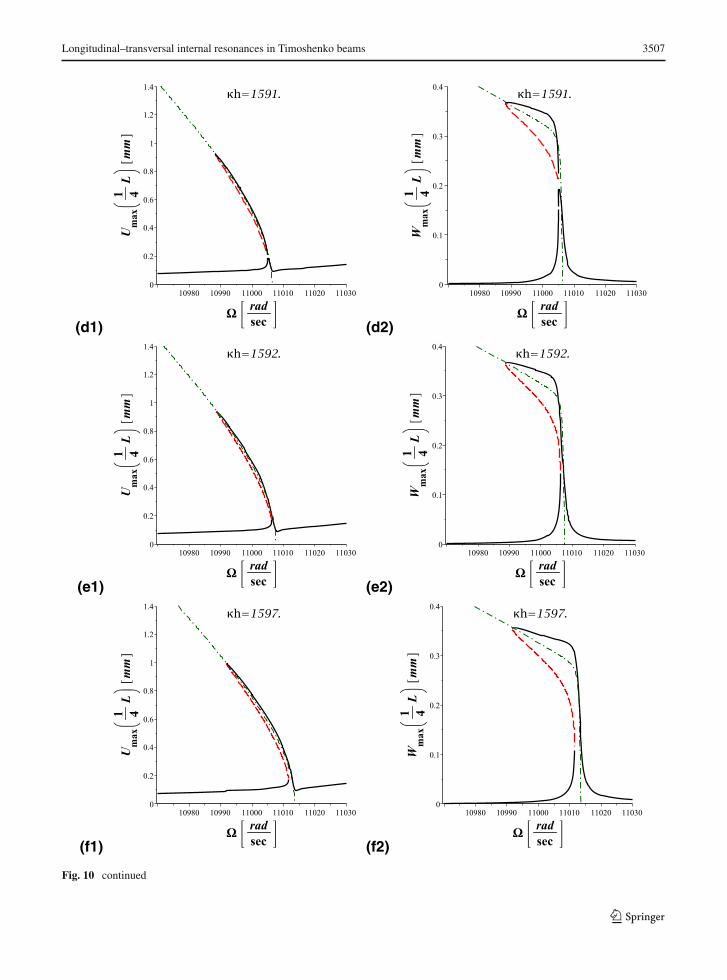
The born of the left resonance curve (see Fig. 9b) isactually more involved than expected, and interesting.An isolated branch of solution, also termed as “isola”,

is born at about κh = 1580 (Fig. 10a, b). By increasingκh , this closed branch enlarges (Fig. 10c, d) and finallytouches, at about κh = 1591.5 (Fig. 10d, e), the non-resonant, small amplitude, branch. Then, a classicalresonant (softening) FRC is observed (Fig. 10f). Thesame phenomenon has been observed, for example, in[35] (see their Fig. 6) and in [36] (see their Fig. 2).

It is just for isolated branches that analytical meth-ods, even approximate, are necessary: here multipletime scales are used, but in other papers (e.g., [37]) iso-las havebeendetectedby the harmonic balancemethod.In fact, they cannot be obtained by a path followingalgorithm starting from themain solution branch unless

123

3506 S. Lenci et al.

(a1) (a2)

(b1) (b2)

(c1) (c2)

Fig. 10 Frequency response curves for Q = 1000 N and dif-ferent values of κh. Continuous black lines are stable solutionbranches, red dashed lines are unstable saddle-type solution

branches, blue dashed lines are unstable source-type solutionbranches. Green dashdot line is the backbone curve ensuing fromωa0/2. (Colours in the online version)

123

Longitudinal–transversal internal resonances in Timoshenko beams 3507

(d1) (d2)

(e1) (e2)

(f1) (f2)

Fig. 10 continued

123

3508 S. Lenci et al.

varying another parameter (for example, the stiffnessof the spring), besides the excitation frequency, whichmay allow to reach isolas in an extended parameterspace. If varying only the excitation frequency, theycan be found numerically only via a suitable and luckychoice of initial values in either the original governingequations or the reduced (e.g., modulated) ones, andthen possibly characterized systematically by build-ing basins of attraction, which is however difficult anddemanding, especially for high dimensional systems.

Detecting stable isolated solutions is not only impor-tant from a theoretical point of view. In fact, even ifthese attractors may have a small basin of attraction,and thus be considered “minor” or “rare”, itmayhappenthat their basins strongly erode, by fractality, the basinof the main attractor (the one used in applications), thatthus loses robustness and reduces its safety, leading toinstability for moderately large perturbations, even ifthe attractor is stable in the Lyapunov sense [38].

6 Numerical simulations

To confirm the previous analytical findings, finite ele-ments method (FEM) simulations are performed. Thesame beam illustrated in Sect. 5 is considered.

The commercial software Abaqus_CAE © is used.The beam is discretized using 100 B21-type elements.An explicit direct time integration is used, with timestep �T = (2π)/( × 80) sec and, to give up thetransient vibration, each excitation lasts 2500 periods.Furthermore, in the solver a double precision is usedtogether with full nodal output precision.

Relatively small changes in (1 rad/s) are used inthe frequency sweeping (both forward and backward),and the solution (shape deformation and rotation angle)obtained in the previous step is used as initial condition,as done in [11].

Axial and transversal dampings proportional to themass matrices are considered, with the same values ofthe damping coefficients used in Sect. 5.

To further confirm our results, we have done com-putations also with another commercial software,Midas_GEN©, but since the outcomes are comparablewe do not report these simulations.

First, the axial and transversal natural frequencieshave been computed in the linear regime, verifyingthat they perfectly match those computed analytically.Then, the FRCs have been obtained in the geometri-

cally nonlinear regime, i.e. with large displacements.Since a brute force following algorithm has been usedto determine the numerical FRC, for increasing anddecreasing frequencies, only the stable branches havebeen detected. To draw also the unstable branches, acontinuation algorithm should have been used, whichis, however, out of the scope of the present work.

The comparison between analytical and numericalresults is reported in Fig. 11, for a fixed value of κ andfor increasing values of Q. We conclude that an excel-lent agreement is obtained on the main (i.e. primaryresonance) stable solution branches. Surprisingly, thepeaks of the numerical curves are higher than those ofthe analytical ones, this being likely due to a differ-ent fine tuning of the damping, that has large effects onthe peak value. Note that no tuning of damping is done,and the nominal values are considered in numerical andanalytical simulations.

Around ωa0/2, we observe that the numerical solu-tion is not able to catch the upper, resonant, stablebranch. This is due to the source-type unstable solutionbranch that breaks the main resonant solution branchand leads to a jump of the theoretical solution. Thenumerical jump is not observed, likely because the solu-tions have very small basins of attraction.

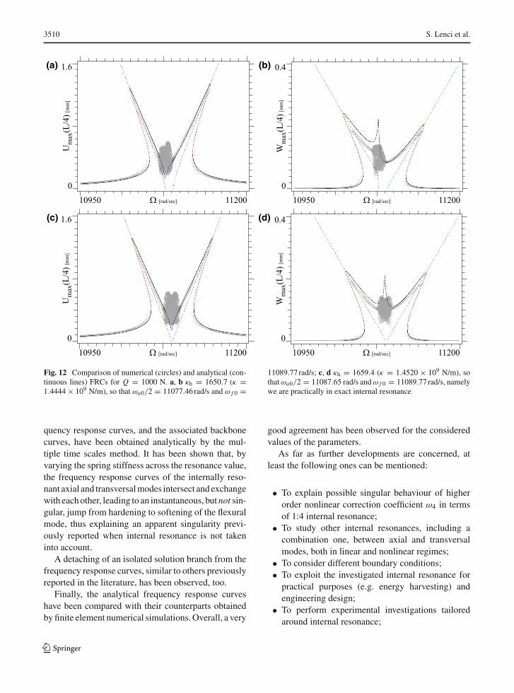
Keeping Q = 1000 N fixed, and varying thespring stiffness, the comparison between analytical andnumerical results is reported in Fig. 12. In additionto the overall excellent agreement, with some minorquantitative differences on W (which can be reducedby tuning the damping), the most important result isthat through the Neimark–Sacker bifurcation a quasi-periodic attractor is born, according to what the theorypredicts for this event [39]. It is highlighted by the cloudof points obtained for each frequency by sampling themaximum amplitudes of the last 500 periods of theexcitation, to give rid of the transient behaviour.

This is a further confirmation of the reliability of theproposed analysis.

7 Conclusions and further developments

The internal resonance between axial and bendingmodes in a Timoshenko beam with a boundary axialspring has been investigated, with the aim (1) of study-ing the ensuing modal interaction in a further mechani-cal system, (2) of explaining a singular behaviour previ-ously reported in the literature, and (3) of investigating

123

Longitudinal–transversal internal resonances in Timoshenko beams 3509

(a)

0

1.6

1120010950 rad/sec

U(L/4)

max

[mm]

(b)

0

0.4

1120010950 rad/sec

W(L/4)

max

[mm]

(c)

0

1.6

1120010950 rad/sec

U(L/4)

max

[mm]

(d)

0

0.4

1120010950 rad/sec

W(L/4)

max

[mm]

(e)

0

1.6

1120010950 rad/sec

U(L/4)

max

[mm]

(f)

0

0.4

1120010950 rad/sec

W(L/4)

max

[mm]

Fig. 11 Comparison of numerical (circles) and analytical (continuous lines) FRCs for κh = 1620 (κ = 1.4175 × 109 N/m). In thiscase, ωa0/2 = 11041.10 rad/s is slightly lesser than ω f 0 = 11089.77 rad/s. a, b Q = 800 N; c, d Q = 1000 N; e, f Q = 1200 N

the transition from softening to hardening through the1 : 2 internal resonance by varying the axial springstiffness.

It has been shown that internal resonance, whilestructurally unstable, is a robust phenomenon, since it

occurs for all values of the end stiffness, and for “any”value of the resonance ratio ir . It is only needed toproperly select the beam length.

Attention has then been paid to the nonlinearbehaviour around the 1 : 2 internal resonance. The fre-

123

3510 S. Lenci et al.

(a)

0

1.6

1120010950 rad/sec

U(L/4)

max

[mm]

(b)

0

0.4

1120010950 rad/sec

W(L/4)

max

[mm]

(c)

0

1.6

1120010950 rad/sec

U(L/4)

max

[mm]

(d)

0

0.4

1120010950 rad/sec

W(L/4)

max

[mm]

Fig. 12 Comparison of numerical (circles) and analytical (con-tinuous lines) FRCs for Q = 1000 N. a, b κh = 1650.7 (κ =1.4444 × 109 N/m), so that ωa0/2 = 11077.46 rad/s and ω f 0 =

11089.77 rad/s; c, d κh = 1659.4 (κ = 1.4520 × 109 N/m), sothatωa0/2 = 11087.65 rad/s andω f 0 = 11089.77 rad/s, namelywe are practically in exact internal resonance

quency response curves, and the associated backbonecurves, have been obtained analytically by the mul-tiple time scales method. It has been shown that, byvarying the spring stiffness across the resonance value,the frequency response curves of the internally reso-nant axial and transversalmodes intersect and exchangewith eachother, leading to an instantaneous, butnot sin-gular, jump from hardening to softening of the flexuralmode, thus explaining an apparent singularity previ-ously reported when internal resonance is not takeninto account.

A detaching of an isolated solution branch from thefrequency response curves, similar to others previouslyreported in the literature, has been observed, too.

Finally, the analytical frequency response curveshave been compared with their counterparts obtainedbyfinite element numerical simulations.Overall, a very

good agreement has been observed for the consideredvalues of the parameters.

As far as further developments are concerned, atleast the following ones can be mentioned:

• To explain possible singular behaviour of higherorder nonlinear correction coefficient ω4 in termsof 1:4 internal resonance;

• To study other internal resonances, including acombination one, between axial and transversalmodes, both in linear and nonlinear regimes;

• To consider different boundary conditions;• To exploit the investigated internal resonance forpractical purposes (e.g. energy harvesting) andengineering design;

• To perform experimental investigations tailoredaround internal resonance;

123

Longitudinal–transversal internal resonances in Timoshenko beams 3511

• To demonstrate that the coupled backbones tend totheir uncoupled counterparts when getting far fromthe resonance.

Acknowledgements The authors thank both anonymousReviewers for bringing to their attention interesting works andfor useful comments. LK and JW would like to acknowledgethe Financial support by grant 2019/33/N/ST8/02661 from theNational Science Centre, Poland. The work of SL and FC is apart of the activities of the “Dipartimento di Eccellenza” of theDICEA, Polytechnic University of Marche.

Funding Open access funding provided by Università Politec-nica delle Marche within the CRUI-CARE Agreement.

Compliance with ethical standards

Conflict of interest SL isAssociate Editor ofNonlinearDynam-ics, although, of course, he has not been involved in themanagingof this work. The authors declare that they have no other conflictsof interest.

Open Access This article is licensed under a Creative Com-mons Attribution 4.0 International License, which permits use,sharing, adaptation, distribution and reproduction in anymediumor format, as long as you give appropriate credit to the originalauthor(s) and the source, provide a link to the Creative Com-mons licence, and indicate if changes were made. The images orother third partymaterial in this article are included in the article’sCreative Commons licence, unless indicated otherwise in a creditline to thematerial. If material is not included in the article’s Cre-ative Commons licence and your intended use is not permitted bystatutory regulation or exceeds the permitted use, you will needto obtain permission directly from the copyright holder. To viewa copy of this licence, visit http://creativecommons.org/licenses/by/4.0/.

Appendix

In this appendix, we report some formulas which arereferred to in the text.

Parameters used in (11):

c1 = −n2π2l2

8

2 zα1 − 2 z + 1

l2 + κh,

c2 = n2π2l2

8

× (2 zα1 − 2 z + 1)(π2l2n2 − 2ω2

0

)(π2l2n2 − ω0

2)[2 cos (2ω0/ l) l ω0 + sin (2ω0/ l) κh]

,

α1 = l4z

π2l2n2 + l4z − ω02 ,

ω2a = −32 l2π2n2(π2n2α2

1

− α21 l

2z + l2z − l2) (

π2n2l2 − ω20

),

ω2b = 16 l4π2n2[π4n4α2

1

− (α21 z − z + 1

) (π2n2l2 − 2ω2

0

)],

ω2c = −π4n4l2{6π2n2

(α31 z

2 − α21 z

2

− α21 z − α1z

2 + z2 + z − 1)l4+

+ [− (4α3

1 z2 − 4α2

1 z2 − 7α2

1 z − 4α1z2

− 2α1z + 4z2 + 9z − 7)ω20+

+ 6π4n4α21 (α1z − z + 1)

]l2

− π2n2α21ω

20 (4α1z − 4z + 5)

},

ω2d = 64ω0(π2n2l2 − ω2

0)(π2n2α2

1 + l2). (49)

Functions used in (23):

W1a(Z) = sin

(x Z

L

),

U1a(Z) = sin

(n π Z

L

),

θ1a(Z) = 1

L

(n π − ω2

0

nπ zl2

)cos

(nπ Z

L

). (50)

Functions used in (30):

fW =(E A

2− GA

)U ′21a + GAU ′

1aθ1a,

fU = (GA − E A)U ′1aW

′1a,

fθ = E J θ ′1aW

′1a . (51)

Parameters used in (31):

r1 =∫ L

0W 2

1adZ = L

2

x − sin(x) cos(x)

x,

r2 =(E A

2− GA

) ∫ L

0W ′

1aU′21adZ

+ GA∫ L

0W ′

1aU′1aθ1adZ =

= E J

L4

sin(x)

2

(2n2π2 − x2)(n2π2l2 − 2ω20)

4n2π2 − x2,

r3 =∫ L

0U 21adZ = L

2,

r4 =∫ L

0θ21adZ =

(n2π2l2z − ω2

0

)22Ln2π2l4z2

,

r5 = −(GA − E A)

∫ L

0W ′

1aU′21adZ

− E J∫ L

0W ′

1aθ′21adZ + GA

∫ L

0W ′

1aθ21adZ

123

3512 S. Lenci et al.

= E J

L4

sin(x)

4n2π2 − x2

[ω20

(2n2π2l2z − ω2

0

)

× 2n4π4 − 2n2π2l2z + l2x2z

n2π2l4z2

−n2π2(2n4π4 − 2n2π2l2 + l2x2

)],

r6 = 1

2

∫ L

0f (Z)U1a(Z)dZ . (52)

References

1. Atluri, S.: Nonlinear vibrations of hinged beam includingnonlinear inertia effects. ASME J. Appl. Mech. 40, 121–126 (1973). https://doi.org/10.1115/1.3422909

2. Luongo, A., Rega, G., Vestroni, F.: On nonlinear dynamicsof planar shear indeformable beams. ASME J. Appl. Mech.53, 619–624 (1986). https://doi.org/10.1115/1.3171821

3. Lacarbonara, W., Yabuno, H.: Refined models of elasticbeams undergoing large in-planemotions: theory and exper-iments. Int. J. Solids Struct. 43, 5066–5084 (2006). https://doi.org/10.1016/j.ijsolstr.2005.07.018

4. Araumi, N., Yabuno, H.: Cubic-quintic nonlinear para-metric resonance of a simply supported beam. Nonlin-ear Dyn. 90, 549–560 (2017). https://doi.org/10.1007/s11071-017-3680-1

5. Lenci, S., Clementi, F., Rega, G.: A comprehensive anal-ysis of hardening/softening behaviour of shearable pla-nar beams with whatever axial boundary constraint. Mec-canica 51(11), 2589–2606 (2016). https://doi.org/10.1007/s11012-016-0374-6

6. Lenci, S., Rega, G.: Nonlinear free vibrations of planar elas-tic beams: a unified treatment of geometrical andmechanicaleffects. Proc. IUTAM 19, 35–42 (2016). https://doi.org/10.1016/j.piutam.2016.03.007

7. Clementi, F., Lenci, S., Rega, G.: Cross-checking asymp-totics and numerics in the hardening/softening behaviour ofTimoshenko beams with axial end spring and variable slen-derness. Arch. Appl. Mech. 87(5), 865–880 (2017). https://doi.org/10.1007/s00419-016-1159-z

8. Lenci, S., Rega, G.: Axial-transversal coupling in the freenonlinear vibrations of Timoshenko beams with arbitraryslenderness and axial boundary conditions. Proc. R. Soc. A472, 20160057 (2016). https://doi.org/10.1098/rspa.2016.0057

9. Lenci, S., Clementi, F., Rega, G.: Comparing nonlinear freevibrations of Timoshenko beams with mechanical or geo-metric curvature definition. Proc. IUTAM 20, 34–41 (2017).https://doi.org/10.1016/j.piutam.2017.03.006

10. Babilio, E., Lenci, S.: On the notion of curvature and itsmechanical meaning in a geometrically exact plane beamtheory. Int. J. Mech. Sci. 128–129, 277–293 (2017). https://doi.org/10.1016/j.ijmecsci.2017.03.031

11. Kloda, L., Lenci, S., Warminski, J.: Nonlinear dynamicsof a planar beam-spring system: analytical and numeri-

cal approaches. Nonlinear Dyn. 94(3), 1721–1738 (2018).https://doi.org/10.1007/s11071-018-4452-2

12. Kloda, L., Lenci, S., Warminski, J.: Hardening vs soften-ing dichotomy of a hinged-simply supported beam with oneend axial linear spring: experimental and numerical studies.Int. J. Mech. Sci. 178, 1–8 (2020). https://doi.org/10.1016/j.ijmecsci.2020.105588

13. Kloda, L., Lenci, S., Warminski, J.: Nonlinear dynamicsof a planar hinged-simply supported beam with one endspring: higher order resonances. In: Kovacic, I., Lenci,S. (eds.) IUTAM Symposium on Exploiting NonlinearDynamics for Engineering Systems, IUTAM Bookseriesvol. 37, pp. 155–165, Springer (2019). https://doi.org/10.1007/978-3-030-23692-2_14

14. Srinil, N., Rega, G.: The effects of kinematic condensationon internally resonant forced vibrations of shallow hori-zontal cables. Int. J. Nonlinear Mech. 42, 180–195 (2007).https://doi.org/10.1016/j.ijnonlinmec.2006.09.005

15. Rega G., Lacarbonara W., Nayfeh A.H.: Reduction meth-ods for nonlinear vibrations of spatially continuous sys-tems with initial curvature. In: Van Dao, N., Kreuzer, E.J.(eds.) IUTAMSymposiumonRecentDevelopments inNon-linear Oscillations ofMechanical Systems, SolidMechanicsand Its Applications, vol. 77, pp. 235–246. Springer (2000).https://doi.org/10.1007/978-94-011-4150-5_24

16. Arafat, H.N., Nayfeh, A.H.: Non-linear responses ofsuspended cables to primary resonance excitations. J.Sound Vib. 266, 325–354 (2003). https://doi.org/10.1016/S0022-460X(02)01393-7

17. Touzé, C., Thomas, O.: Non-linear behaviour of free-edgeshallow spherical shells: effect of the geometry. Int. J. Non-linear Mech. 41, 678–692 (2006). https://doi.org/10.1016/j.ijnonlinmec.2005.12.004

18. Touzé, C., Amabili, M.: Nonlinear normal modes fordamped geometrically nonlinear systems: Application toreduced-order modelling of harmonically forced structures.J. SoundVib. 298, 958–981 (2006). https://doi.org/10.1016/j.jsv.2006.06.032

19. Chen, L.-Q., Zhang, Y.-L., Zhang, G.-C., Ding, H.: Evolu-tion of the double-jumping in pipes conveying fluid flowingat the supercritical speed. Int. J. Nonlinear Mech. 58, 11–21(2014). https://doi.org/10.1016/j.ijnonlinmec.2013.08.012

20. Chen, L.-Q., Zhang, G.-C., Ding, H.: Internal resonance inforced vibration of coupled cantilevers subjected to mag-netic interaction. J. SoundVib. 354, 196–218 (2015). https://doi.org/10.1016/j.jsv.2015.06.010

21. Nayfeh, A.H., Balachandran, B.: Modal interactions indynamical and structural systems. ASME Appl. Mech. Rev.42, S175–S201 (1989). https://doi.org/10.1115/1.3152389

22. Bajaj, A.K., Davies, P., Chang, S.I.: On internal resonancesin mechanical systems. In: Kliemann, W. (ed.) NonlinearDynamics and Stochastic Mechanics, CRC Press (1995) (e-version 2018)

23. Manevich, A.I., Manevitch, L.I.: Mechanics of NonlinearSystems with Internal Resonances. Imperial College Press,London (2003)

24. Nayfeh, A.H., Pai, P.F.: Linear and Nonlinear StructuralMechanics. Wiley, New York (2007)

25. Arioli, G., Gazzola, F.: A new mathematical explanationof what triggered the catastrophic torsional mode of the

123

Longitudinal–transversal internal resonances in Timoshenko beams 3513

Tacoma Narrows Bridge. Appl. Math. Modell. 39, 901–912(2015). https://doi.org/10.1016/j.apm.2014.06.022

26. Jiang, W.-A., Chen, L.-Q., Ding, H.: Internal resonance inaxially loaded beam energy harvesters with an oscillatorto enhance the bandwidth. Nonlinear Dyn. 85, 2507–2520(2016). https://doi.org/10.1007/s11071-016-2841-y

27. Leamy, M.J., Gottlieb, O.: Internal resonances in whirlingstrings involving longitudinal dynamics and material non-linearities. J. Sound Vib. 236(4), 683–703 (2000). https://doi.org/10.1006/jsvi.2000.3039

28. Srinil, N., Rega, G.: Nonlinear longitudinal/transversalmodal interactions in highly extensible suspended cables. J.Sound Vib. 310, 230–242 (2008). https://doi.org/10.1016/j.jsv.2007.07.056

29. Scurtu, P.R., Clark, M., Zu, J.W.: Coupled longitudinaland transverse vibration of automotive belts under longi-tudinal excitations using analog equation method. J. Vib.Control 18(9), 1336–1352 (2011). https://doi.org/10.1177/1077546311418866

30. Yang,X.-D.,Zhang,W.:Nonlinear dynamics of axiallymov-ing beam with coupled longitudinal-transversal vibrations.Nonlinear Dyn. 78, 2547–2556 (2014). https://doi.org/10.1007/s11071-014-1609-5

31. Ma, C., Cao, L., Li, L., Shao, M., Jing, D., Guo, Z.: Nonlin-ear behaviour of electrostatically actuated microbeams withcoupled longitudinal-transversal vibration. Micromachines10(5), 315 (2019). https://doi.org/10.3390/mi10050315

32. Kloda, L.: Coupled Longitudinal–Transversal Vibrations ofa Nonlinear Planar Timoshenko Beam with an Axial EndSpring. Polytechnic University of Marche, Ancona (2020).PhD Thesis

33. Touzé, C., Thomas, O., Chaigne, A.: Hardening/softeningbehaviour in non-linear oscillations of structural systemsusing non-linear normalmodes. J. SoundVib. 273(1–2), 77–101 (2004). https://doi.org/10.1016/j.jsv.2003.04.005

34. Nayfeh, A.: Introduction to Perturbation Techniques. Wiley,New York (2004)

35. Detroux, T., Noël, J.P., Virgin, L.N., Kerschen, G.: Experi-mental study of isolas in nonlinear systems featuring modalinteractions. PLoS ONE 13(3), e0194452 (2018). https://doi.org/10.1371/journal.pone.0194452

36. Mangussi, F., Zanette, D.H.: Internal resonance in a vibrat-ing beam: a zoo of nonlinear resonance peaks. PLoS ONE11(9), e0162365 (2016). https://doi.org/10.1371/journal.pone.0162365

37. Salles, L., Staples, B., Hoffmann, N., Schwingshackl, C.:Continuation techniques for analysis of whole aeroenginedynamicswith imperfect bifurcations and isolated solutions.Nonlinear Dyn. 86, 1897–1911 (2016). https://doi.org/10.1007/s11071-016-3003-y

38. Lenci, S., Rega, G.: Global Nonlinear Dynamics for Engi-neering Design and System Safety. Springer, New York(2019)

39. Wiggins, S.: Introduction to Applied Nonlinear DynamicalSystems and Chaos, 2nd edn. Springer, New York (2003)

Publisher’s Note Springer Nature remains neutral with regardto jurisdictional claims in published maps and institutional affil-iations.

123