Long time approximation and modi ed equations for SDEs

Long time approximation and modifiedequations for SDEs

Tony [email protected]

The University of Manchester

August 2011

1 / 1

Outline

1 Modified Equations

2 SDEs and long time approximation

3 Modified equations for SDEs

4 Modified equations and long time approximation

5 Conclusions and open problems

2 / 1

Outline






3 / 1

What is a modified equation?

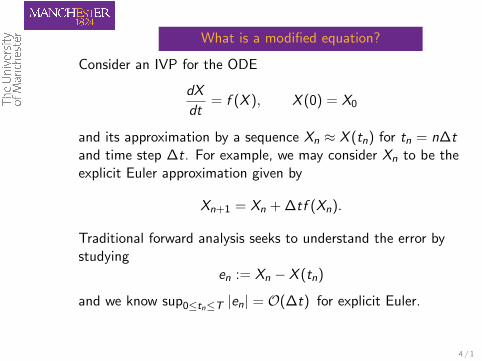
Consider an IVP for the ODE

dX

dt= f (X ), X (0) = X0

and its approximation by a sequence Xn ≈ X (tn) for tn = n∆tand time step ∆t. For example, we may consider Xn to be theexplicit Euler approximation given by

Xn+1 = Xn + ∆tf (Xn).

Traditional forward analysis seeks to understand the error bystudying

en := Xn − X (tn)

and we know sup0≤tn≤T |en| = O(∆t) for explicit Euler.

4 / 1

Backward error analysis

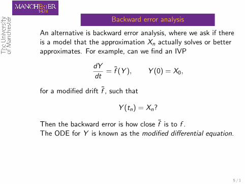
An alternative is backward error analysis, where we ask if thereis a model that the approximation Xn actually solves or betterapproximates. For example, can we find an IVP

dY

dt= f̃ (Y ), Y (0) = X0,

for a modified drift f̃ , such that

Y (tn) = Xn?

Then the backward error is how close f̃ is to f .The ODE for Y is known as the modified differential equation.

5 / 1

Simple example

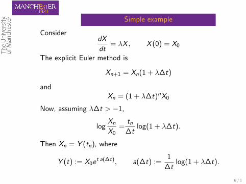
ConsiderdX

dt= λX , X (0) = X0

The explicit Euler method is

Xn+1 = Xn(1 + λ∆t)

andXn = (1 + λ∆t)nX0

Now, assuming λ∆t > −1,

logXn

X0=

tn∆t

log(1 + λ∆t).

Then Xn = Y (tn), where

Y (t) := X0et a(∆t), a(∆t) :=1

∆tlog(1 + λ∆t).

6 / 1

Continued.

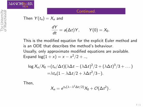
Then Y (tn) = Xn and

dY

dt= a(∆t)Y , Y (0) = X0.

This is the modified equation for the explicit Euler method andis an ODE that describes the method’s behaviour.Usually, only approximate modified equations are available.Expand log(1 + x) = x − x2/2 + ..,

log Xn/X0 =(tn/∆t)(λ∆t − (λ∆t)2/2 + (λ∆t)3/3 + . . . )

=λtn(1− λ∆t/2 + λ∆t2/3−).

Then,Xn = etn(λ−λ2∆t/2)X0 +O(∆t2) .

7 / 1

Continued.

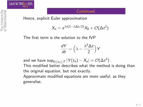
Hence, explicit Euler approximation

Xn = eλt(1−λ∆t/2)X0 +O(∆t2)

The first term is the solution to the IVP

dY

dt=(λ− λ2∆t

2

)Y

and we have sup0≤tn≤T |Y (tn)− Xn| = O(∆t2) .This modified better describes what the method is doing thanthe original equation, but not exactly.Approximate modified equations are more useful, as theygeneralise.

8 / 1

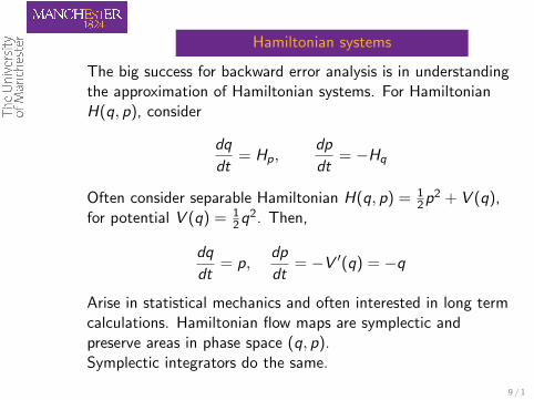
Hamiltonian systems

The big success for backward error analysis is in understandingthe approximation of Hamiltonian systems. For HamiltonianH(q, p), consider

dq

dt= Hp,

dp

dt= −Hq

Often consider separable Hamiltonian H(q, p) = 12 p2 + V (q),

for potential V (q) = 12 q2. Then,

dq

dt= p,

dp

dt= −V ′(q) = −q

Arise in statistical mechanics and often interested in long termcalculations. Hamiltonian flow maps are symplectic andpreserve areas in phase space (q, p).Symplectic integrators do the same.

9 / 1

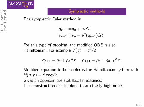
Symplectic methods

The symplectic Euler method is

qn+1 =qn + pn∆t

pn+1 =pn − V ′(qn+1)∆t

For this type of problem, the modified ODE is alsoHamiltonian. For example V (q) = q2/2

qn+1 = qn + pn∆t; pn+1 = pn − qn+1∆t

Modified equation to first order is the Hamiltonian system withH(q, p)−∆tpq/2.Gives an approximate statistical mechanics.This construction can be done to arbitrarily high order.

10 / 1

Outline






11 / 1

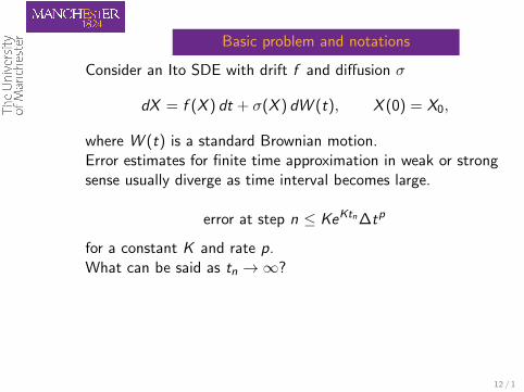
Basic problem and notations

Consider an Ito SDE with drift f and diffusion σ

dX = f (X ) dt + σ(X ) dW (t), X (0) = X0,

where W (t) is a standard Brownian motion.Error estimates for finite time approximation in weak or strongsense usually diverge as time interval becomes large.

error at step n ≤ KeKtn∆tp

for a constant K and rate p.What can be said as tn →∞?

12 / 1

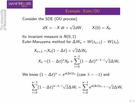
Example: Euler/OU

Consider the SDE (OU process)

dX = −X dt +√

2dW , X (0) = X0.

Its invariant measure is N(0, 1).Euler-Maruyama method for ∆Wn = W (tn+1)−W (tn),

Xn+1 =Xn(1−∆t) +√

2∆Wn

Xn =(1−∆t)nX0 +n−1∑i=0

(1−∆t)n−1−i√2∆Wi .

We know (1−∆t)n = ea(∆t)tn (case λ = −1) and

n−1∑i=0

(1−∆t)n−1−i√2∆Wi =n−1∑i=0

ea(∆t)tn−1−i√

2∆Wi

13 / 1

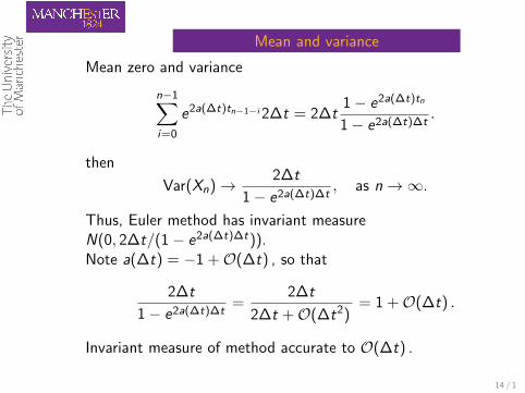
Mean and variance

Mean zero and variance

n−1∑i=0

e2a(∆t)tn−1−i 2∆t = 2∆t1− e2a(∆t)tn

1− e2a(∆t)∆t.

then

Var(Xn)→ 2∆t

1− e2a(∆t)∆t, as n→∞.

Thus, Euler method has invariant measureN(0, 2∆t/(1− e2a(∆t)∆t)).Note a(∆t) = −1 +O(∆t) , so that

2∆t

1− e2a(∆t)∆t=

2∆t

2∆t +O(∆t2)= 1 +O(∆t) .

Invariant measure of method accurate to O(∆t) .

14 / 1

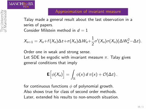
Approximation of invariant measure

Talay made a general result about the last observation in aseries of papers.Consider Milstein method in d = 1

Xn+1 = Xn+f (Xn)∆t+σ(Xn)∆Wn+1

2σ′(Xn)σ(Xn)(∆W 2

n−∆t).

Order one in weak and strong sense.Let SDE be ergodic with invariant measure π. Talay givesgeneral conditions that imply

E[φ(Xn)

]=

∫Rφ(x) d π(x) +O(∆t) .

for continuous functions φ of polynomial growth.Also shows true for class of second order methods.Later, extended his results to non-smooth situation.

15 / 1

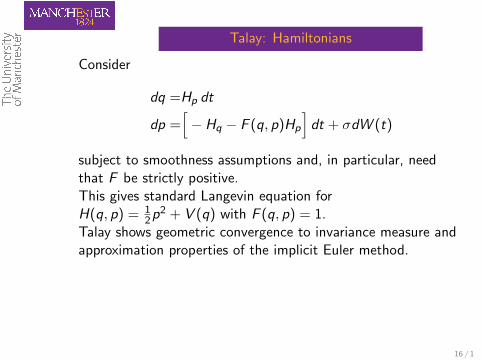
Talay: Hamiltonians

Consider

dq =Hp dt

dp =[− Hq − F (q, p)Hp

]dt + σdW (t)

subject to smoothness assumptions and, in particular, needthat F be strictly positive.This gives standard Langevin equation forH(q, p) = 1

2 p2 + V (q) with F (q, p) = 1.Talay shows geometric convergence to invariance measure andapproximation properties of the implicit Euler method.

16 / 1

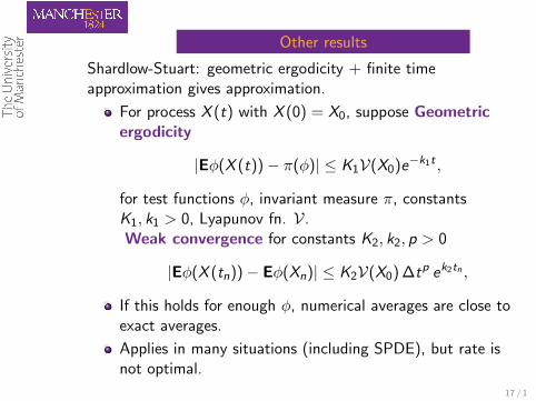
Other results

Shardlow-Stuart: geometric ergodicity + finite timeapproximation gives approximation.

For process X (t) with X (0) = X0, suppose Geometricergodicity

|Eφ(X (t))− π(φ)| ≤ K1V(X0)e−k1t ,

for test functions φ, invariant measure π, constantsK1, k1 > 0, Lyapunov fn. V.Weak convergence for constants K2, k2, p > 0

|Eφ(X (tn))− Eφ(Xn)| ≤ K2V(X0) ∆tp ek2tn ,

If this holds for enough φ, numerical averages are close toexact averages.

Applies in many situations (including SPDE), but rate isnot optimal.

17 / 1

Outline






18 / 1

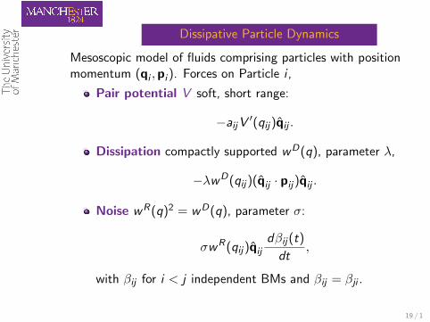
Dissipative Particle Dynamics

Mesoscopic model of fluids comprising particles with positionmomentum (qi ,pi ). Forces on Particle i ,

Pair potential V soft, short range:

−aijV′(qij)q̂ij .

Dissipation compactly supported wD(q), parameter λ,

−λwD(qij)(q̂ij · pij)q̂ij .

Noise wR(q)2 = wD(q), parameter σ:

σwR(qij)q̂ij

dβij(t)

dt,

with βij for i < j independent BMs and βij = βji .

19 / 1

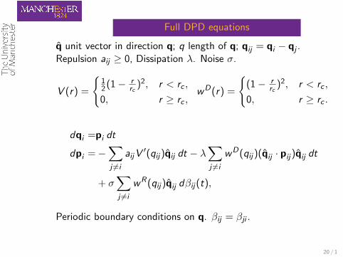
Full DPD equations

q̂ unit vector in direction q; q length of q; qij = qi − qj .Repulsion aij ≥ 0, Dissipation λ. Noise σ.

V (r) =

{12 (1− r

rc)2, r < rc ,

0, r ≥ rc ,wD(r) =

{(1− r

rc)2, r < rc ,

0, r ≥ rc .

dqi =pi dt

dpi =−∑j 6=i

aijV′(qij)q̂ij dt − λ

∑j 6=i

wD(qij)(q̂ij · pij)q̂ij dt

+ σ∑j 6=i

wR(qij)q̂ij dβij(t),

Periodic boundary conditions on q. βij = βji .

20 / 1

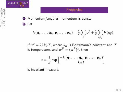
Properties

1 Momentum/angular momentum is const.

2 Let

H(q1, . . . ,qN ,p1, . . . ,pN) = 12

∑i

p2i + 1

2

∑i 6=j

V (qij)

If σ2 = 2λkBT , where kB is Boltzmann’s constant and Tis temperature, and wD = (wR)2, then

ρ =1

Zexp

[−H(q1, . . . ,qN ,p1, . . . ,pN)

kBT

]is invariant measure.

21 / 1

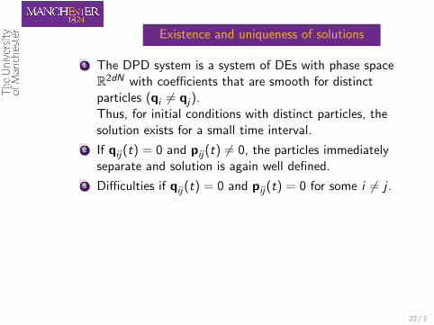
Existence and uniqueness of solutions

1 The DPD system is a system of DEs with phase spaceR2dN with coefficients that are smooth for distinctparticles (qi 6= qj).Thus, for initial conditions with distinct particles, thesolution exists for a small time interval.

2 If qij(t) = 0 and pij(t) 6= 0, the particles immediatelyseparate and solution is again well defined.

3 Difficulties if qij(t) = 0 and pij(t) = 0 for some i 6= j .

22 / 1

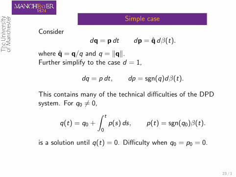
Simple case

Considerdq = p dt dp = q̂ dβ(t).

where q̂ = q/q and q = ‖q‖.Further simplify to the case d = 1,

dq = p dt, dp = sgn(q)dβ(t).

This contains many of the technical difficulties of the DPDsystem. For q0 6= 0,

q(t) = q0 +

∫ t

0p(s) ds, p(t) = sgn(q0)β(t).

is a solution until q(t) = 0. Difficulty when q0 = p0 = 0.

23 / 1

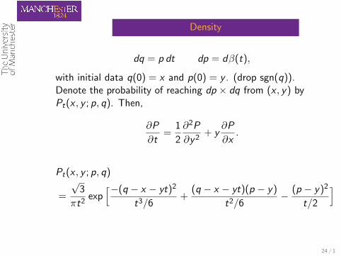
Density

dq = p dt dp = dβ(t),

with initial data q(0) = x and p(0) = y . (drop sgn(q)).Denote the probability of reaching dp × dq from (x , y) byPt(x , y ; p, q). Then,

∂P

∂t=

1

2

∂2P

∂y 2+ y

∂P

∂x.

Pt(x , y ; p, q)

=

√3

πt2exp

[−(q − x − yt)2

t3/6+

(q − x − yt)(p − y)

t2/6− (p − y)2

t/2

]

24 / 1

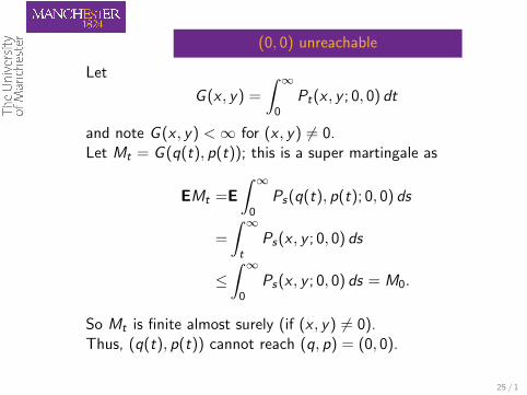
(0, 0) unreachable

Let

G (x , y) =

∫ ∞0

Pt(x , y ; 0, 0) dt

and note G (x , y) <∞ for (x , y) 6= 0.Let Mt = G (q(t), p(t)); this is a super martingale as

EMt =E

∫ ∞0

Ps(q(t), p(t); 0, 0) ds

=

∫ ∞t

Ps(x , y ; 0, 0) ds

≤∫ ∞

0Ps(x , y ; 0, 0) ds = M0.

So Mt is finite almost surely (if (x , y) 6= 0).Thus, (q(t), p(t)) cannot reach (q, p) = (0, 0).

25 / 1

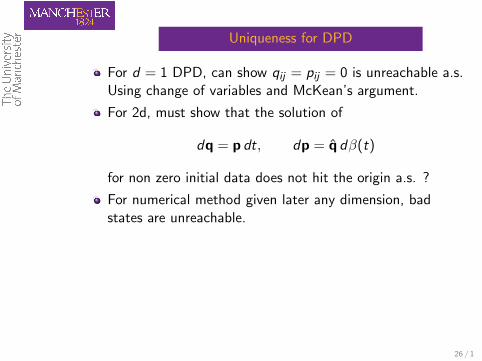
Uniqueness for DPD

For d = 1 DPD, can show qij = pij = 0 is unreachable a.s.Using change of variables and McKean’s argument.

For 2d, must show that the solution of

dq = p dt, dp = q̂ dβ(t)

for non zero initial data does not hit the origin a.s. ?

For numerical method given later any dimension, badstates are unreachable.

26 / 1

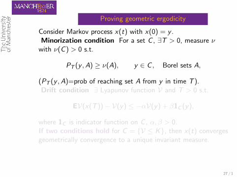
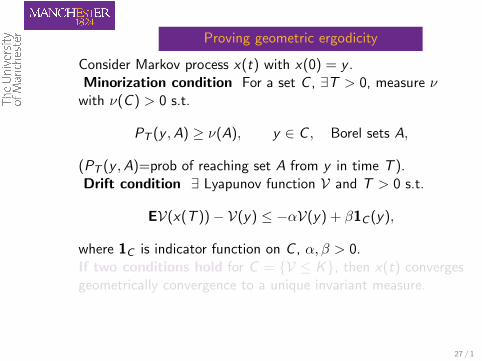
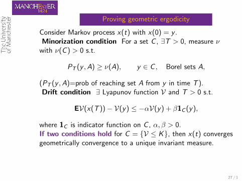
Proving geometric ergodicity

Consider Markov process x(t) with x(0) = y .Minorization condition For a set C , ∃T > 0, measure ν

with ν(C ) > 0 s.t.

PT (y ,A) ≥ ν(A), y ∈ C , Borel sets A,

(PT (y ,A)=prob of reaching set A from y in time T ).Drift condition ∃ Lyapunov function V and T > 0 s.t.

EV(x(T ))− V(y) ≤ −αV(y) + β1C (y),

where 1C is indicator function on C , α, β > 0.If two conditions hold for C = {V ≤ K}, then x(t) convergesgeometrically convergence to a unique invariant measure.

27 / 1






EV(x(T ))− V(y) ≤ −αV(y) + β1C (y),


27 / 1






EV(x(T ))− V(y) ≤ −αV(y) + β1C (y),


27 / 1

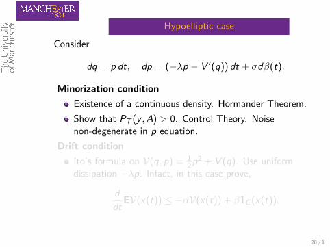
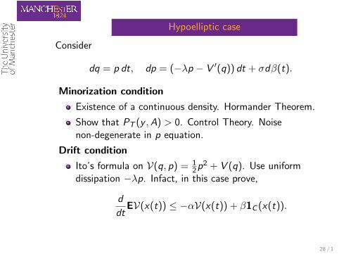
Hypoelliptic case

Consider

dq = p dt, dp = (−λp − V ′(q)) dt + σdβ(t).

Minorization condition

Existence of a continuous density. Hormander Theorem.

Show that PT (y ,A) > 0. Control Theory. Noisenon-degenerate in p equation.

Drift condition

Ito’s formula on V(q, p) = 12 p2 + V (q). Use uniform

dissipation −λp. Infact, in this case prove,

d

dtEV(x(t)) ≤ −αV(x(t)) + β1C (x(t)).

28 / 1

Hypoelliptic case

Consider

dq = p dt, dp = (−λp − V ′(q)) dt + σdβ(t).


Existence of a continuous density. Hormander Theorem.

Show that PT (y ,A) > 0. Control Theory. Noisenon-degenerate in p equation.

Drift condition

Ito’s formula on V(q, p) = 12 p2 + V (q). Use uniform

dissipation −λp. Infact, in this case prove,

d

dtEV(x(t)) ≤ −αV(x(t)) + β1C (x(t)).

28 / 1

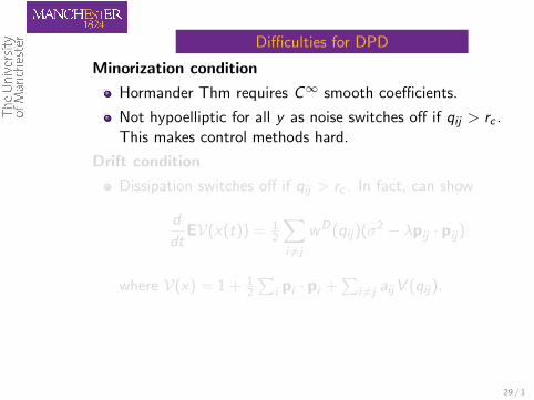
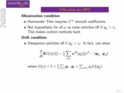
Difficulties for DPD


Hormander Thm requires C∞ smooth coefficients.

Not hypoelliptic for all y as noise switches off if qij > rc .This makes control methods hard.

Drift condition

Dissipation switches off if qij > rc . In fact, can show

d

dtEV(x(t)) = 1

2

∑i 6=j

wD(qij)(σ2 − λpij · pij)

where V(x) = 1 + 12

∑i pi · pi +

∑i 6=j aijV (qij).

29 / 1

Difficulties for DPD


Hormander Thm requires C∞ smooth coefficients.

Not hypoelliptic for all y as noise switches off if qij > rc .This makes control methods hard.

Drift condition

Dissipation switches off if qij > rc . In fact, can show

d

dtEV(x(t)) = 1

2

∑i 6=j

wD(qij)(σ2 − λpij · pij)

where V(x) = 1 + 12

∑i pi · pi +

∑i 6=j aijV (qij).

29 / 1

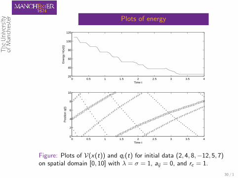
Plots of energy

0 0.5 1 1.5 2 2.5 3 3.5 420

40

60

80

100

120

Time t

Ene

rgy

H(x

(t))

0 0.5 1 1.5 2 2.5 3 3.5 40

2

4

6

8

10

Time t

Pos

ition

q(t

)

Figure: Plots of V(x(t)) and qi (t) for initial data (2, 4, 8,−12, 5, 7)on spatial domain [0, 10] with λ = σ = 1, aij = 0, and rc = 1.

30 / 1

Working with DPD

Drift condition

Prove that collisions of two particles gives rise togeometric decay on a time interval length dt.

Prove that collisions of particles happen sufficiently often.


Coefficients are smooth except at bad points qi = qj .Apply Hormander on a non-characteristic subdomain withabsorbing BCs (Cattiaux, 1991), to get lower bound ontransition density.

Assume domain length L < Nrc , then at least one pair willinteract and can start a control argument.

31 / 1

Working with DPD

Drift condition

Prove that collisions of two particles gives rise togeometric decay on a time interval length dt.

Prove that collisions of particles happen sufficiently often.


Coefficients are smooth except at bad points qi = qj .Apply Hormander on a non-characteristic subdomain withabsorbing BCs (Cattiaux, 1991), to get lower bound ontransition density.

Assume domain length L < Nrc , then at least one pair willinteract and can start a control argument.

31 / 1

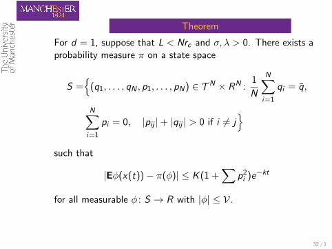
Theorem

For d = 1, suppose that L < Nrc and σ, λ > 0. There exists aprobability measure π on a state space

S ={

(q1, . . . , qN , p1, . . . , pN) ∈ T N × RN :1

N

N∑i=1

qi = q̄,

N∑i=1

pi = 0, |pij |+ |qij | > 0 if i 6= j}

such that

|Eφ(x(t))− π(φ)| ≤ K (1 +∑

p2i )e−kt

for all measurable φ : S → R with |φ| ≤ V.

32 / 1

In two/three dimensions?

Many difficulties:

Pathwise uniqueness.

Geometry harder, as particles may move parallel to oneanother and not collide.

A single pair interaction gives noise in one dimension. Soneed at least two pair interactions for noise to span thetwo dimensions of p.

33 / 1

Outline






34 / 1

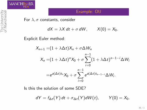
Example: OU

For λ, σ constants, consider

dX = λX dt + σ dW , X (0) = X0.

Explicit Euler method:

Xn+1 =(1 + λ∆t)Xn + σ∆Wn

Xn =(1 + λ∆t)nX0 + σ

n−1∑i=0

(1 + λ∆t)n−1−i∆Wi

=ea(∆t)tnX0 + σ

n−1∑i=0

ea(∆t)tn−1−i ∆Wi .

Is this the solution of some SDE?

dY = f∆t(Y ) dt + σ∆t(Y )dW (t), Y (0) = X0.

35 / 1

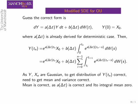
Modified SDE for OU

Guess the correct form is

dY = a(∆t)Y dt + b(∆t) dW (t), Y (0) = X0.

where a(∆t) is already derived for deterministic case. Then,

Y (tn) =ea(∆t)tnX0 + b(∆t)

∫ tn

0ea(∆t)(tn−s) dW (s)

=ea(∆t)tnX0 + b(∆t)n−1∑i=0

∫ ti+1

ti

ea(∆t)(tn−s) dW (s).

As Y , Xn are Gaussian, to get distribution of Y (tn) correct,need to get mean and variance correct.Mean is correct, as a(∆t) is correct and Ito integral mean zero.

36 / 1

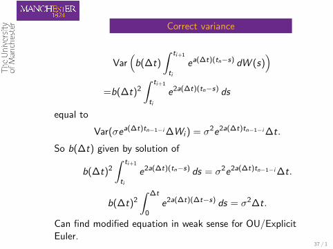
Correct variance

Var(

b(∆t)

∫ ti+1

ti

ea(∆t)(tn−s) dW (s))

=b(∆t)2

∫ ti+1

ti

e2a(∆t)(tn−s) ds

equal to

Var(σea(∆t)tn−1−i ∆Wi ) = σ2e2a(∆t)tn−1−i ∆t.

So b(∆t) given by solution of

b(∆t)2

∫ ti+1

ti

e2a(∆t)(tn−s) ds = σ2e2a(∆t)tn−1−i ∆t.

b(∆t)2

∫ ∆t

0e2a(∆t)(∆t−s) ds = σ2∆t.

Can find modified equation in weak sense for OU/ExplicitEuler.

37 / 1

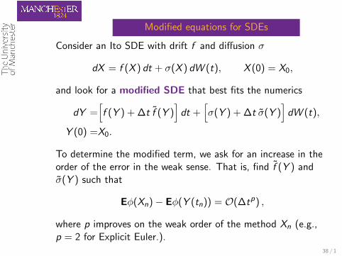
Modified equations for SDEs

Consider an Ito SDE with drift f and diffusion σ

dX = f (X ) dt + σ(X ) dW (t), X (0) = X0,

and look for a modified SDE that best fits the numerics

dY =[f (Y ) + ∆t f̃ (Y )

]dt +

[σ(Y ) + ∆t σ̃(Y )

]dW (t),

Y (0) =X0.

To determine the modified term, we ask for an increase in theorder of the error in the weak sense. That is, find f̃ (Y ) andσ̃(Y ) such that

Eφ(Xn)− Eφ(Y (tn)) = O(∆tp) ,

where p improves on the weak order of the method Xn (e.g.,p = 2 for Explicit Euler.).

38 / 1

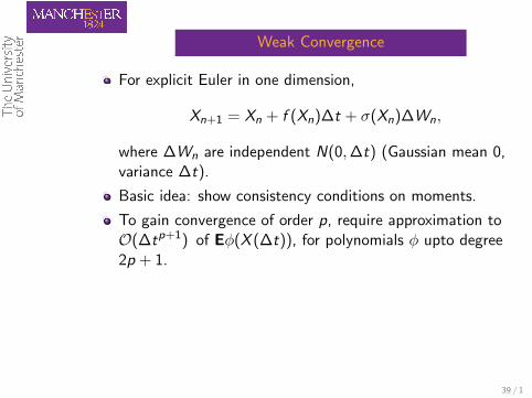
Weak Convergence

For explicit Euler in one dimension,

Xn+1 = Xn + f (Xn)∆t + σ(Xn)∆Wn,

where ∆Wn are independent N(0,∆t) (Gaussian mean 0,variance ∆t).

Basic idea: show consistency conditions on moments.

To gain convergence of order p, require approximation toO(∆tp+1) of Eφ(X (∆t)), for polynomials φ upto degree2p + 1.

39 / 1

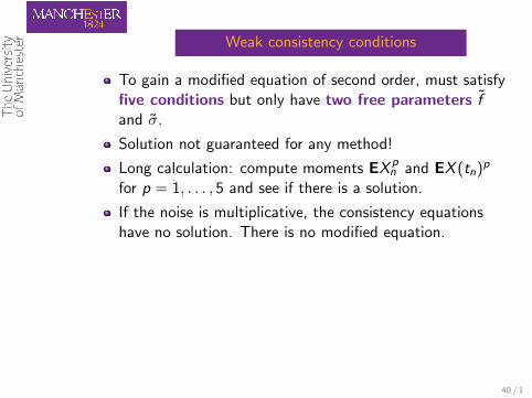
Weak consistency conditions

To gain a modified equation of second order, must satisfyfive conditions but only have two free parameters f̃and σ̃.

Solution not guaranteed for any method!

Long calculation: compute moments EX pn and EX (tn)p

for p = 1, . . . , 5 and see if there is a solution.

If the noise is multiplicative, the consistency equationshave no solution. There is no modified equation.

40 / 1

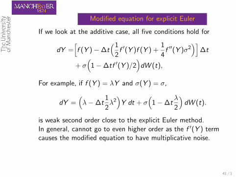
Modified equation for explicit Euler

If we look at the additive case, all five conditions hold for

dY =[f (Y )−∆t

(1

2f ′(Y )f (Y ) +

1

4f ′′(Y )σ2

)]∆t

+ σ(

1−∆tf ′(Y )/2)

dW (t),

For example, if f (Y ) = λY and σ(Y ) = σ,

dY =(λ−∆t

1

2λ2)

Y dt + σ(

1−∆tλ

2

)dW (t).

is weak second order close to the explicit Euler method.In general, cannot go to even higher order as the f ′(Y ) termcauses the modified equation to have multiplicative noise.

41 / 1

Extensions: explicit Euler

In R2, there are now twenty moments conditions.It is possible to find a second order modified SDE forexplicit Euler in this case.

∞-modified equation for Gaussian cases (like OU andexplicit Euler). Already derived.

Zygalakis, developed ∞ modified equation and introducesa technique based on the generator, which simplifiescalculations.

42 / 1

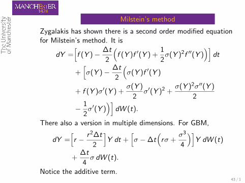
Milstein’s method

Zygalakis has shown there is a second order modified equationfor Milstein’s method. It is

dY =[f (Y )− ∆t

2

(f (Y )f ′(Y ) +

1

2σ(Y )2f ′′(Y )

)]dt

+[σ(Y )− ∆t

2

(σ(Y )f ′(Y )

+ f (Y )σ′(Y ) +σ(Y )

2σ′(Y )2 +

σ(Y )2σ′′(Y )

2

− 1

2σ′(Y )

)]dW (t).

There also a version in multiple dimensions. For GBM,

dY =[r − r 2∆t

2

]Y dt +

[σ −∆t

(rσ +

σ3

4

)]Y dW (t)

+∆t

4σ dW (t).

Notice the additive term.43 / 1

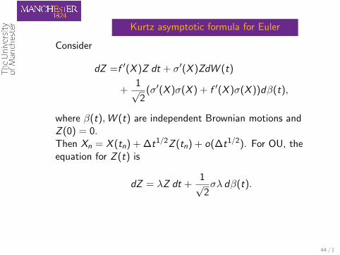
Kurtz asymptotic formula for Euler

Consider

dZ =f ′(X )Z dt + σ′(X )ZdW (t)

+1√2

(σ′(X )σ(X ) + f ′(X )σ(X ))dβ(t),

where β(t),W (t) are independent Brownian motions andZ (0) = 0.Then Xn = X (tn) + ∆t1/2Z (tn) + o(∆t1/2). For OU, theequation for Z (t) is

dZ = λZ dt +1√2σλ dβ(t).

44 / 1

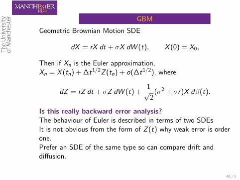
GBM

Geometric Brownian Motion SDE

dX = rX dt + σX dW (t), X (0) = X0,

Then if Xn is the Euler approximation,Xn = X (tn) + ∆t1/2Z (tn) + o(∆t1/2), where

dZ = rZ dt + σZ dW (t) +1√2

(σ2 + σr)X dβ(t).

Is this really backward error analysis?The behaviour of Euler is described in terms of two SDEsIt is not obvious from the form of Z (t) why weak error is orderone.Prefer an SDE of the same type so can compare drift anddiffusion.

45 / 1

Outline






46 / 1

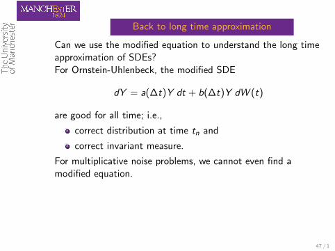
Back to long time approximation

Can we use the modified equation to understand the long timeapproximation of SDEs?For Ornstein-Uhlenbeck, the modified SDE

dY = a(∆t)Y dt + b(∆t)Y dW (t)

are good for all time; i.e.,

correct distribution at time tn and

correct invariant measure.

For multiplicative noise problems, we cannot even find amodified equation.

47 / 1

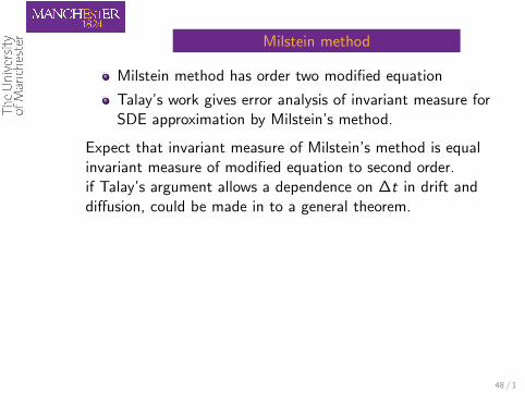
Milstein method

Milstein method has order two modified equation

Talay’s work gives error analysis of invariant measure forSDE approximation by Milstein’s method.

Expect that invariant measure of Milstein’s method is equalinvariant measure of modified equation to second order.if Talay’s argument allows a dependence on ∆t in drift anddiffusion, could be made in to a general theorem.

48 / 1

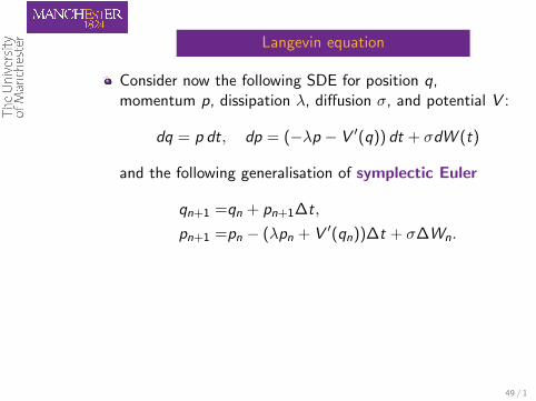
Langevin equation

Consider now the following SDE for position q,momentum p, dissipation λ, diffusion σ, and potential V :

dq = p dt, dp = (−λp − V ′(q)) dt + σdW (t)

and the following generalisation of symplectic Euler

qn+1 =qn + pn+1∆t,

pn+1 =pn − (λpn + V ′(qn))∆t + σ∆Wn.

49 / 1

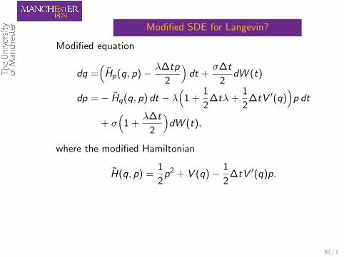
Modified SDE for Langevin?

Modified equation

dq =(

H̃p(q, p)− λ∆tp

2

)dt +

σ∆t

2dW (t)

dp =− H̃q(q, p) dt − λ(

1 +1

2∆tλ+

1

2∆tV ′(q)

)p dt

+ σ(

1 +λ∆t

2

)dW (t),

where the modified Hamiltonian

H̃(q, p) =1

2p2 + V (q)− 1

2∆tV ′(q)p.

50 / 1

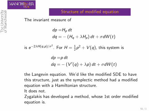
Structure of modified equation

The invariant measure of

dp =Hp dt

dq =− (Hq + λHp) dt + σdW (t)

is e−2λH(q,p)/σ2. For H = 1

2 p2 + V (q), this system is

dp =p dt

dq =− (V ′(q) + λp) dt + σdW (t)

the Langevin equation. We’d like the modified SDE to havethis structure, just as the symplectic method had a modifiedequation with a Hamiltonian structure.It does not.Zygalakis has developed a method, whose 1st order modifiedequation is.

51 / 1

Outline






52 / 1

Conclusions

1 Long time error analysis for SDEs well developed,especially Talay and coworkers.

2 Euler additive SDE, can write down modified equation tohigh order.

3 Milstein has second order modified equation.

4 For Langevin equation, symplectic Euler has modifiedequation but not appropriate structure. Zygalakis gives amethod where Langevin structure is found in modifiedequation.

5 Is there a pathwise modified equation? Certainly need tostep outside SDEs of the same type to do this.

6 Perhaps, use rough path space analysis to consider SDEsforced by some appropriate rough path?

7 Relate modifed equation to asymptotic analysis.

53 / 1

Documents

Long time approximation and modi ed equations for SDEs