Long-Term Investing Strategies in Private Wealth Management

July 2012

Noël AmencProfessor of Finance, EdhEc Business School and director, EdhEc-Risk Institute

Romain DeguestSenior Research Engineer, EdhEc-Risk Institute

Lionel MartelliniProfessor of Finance, EdhEc Business School and Scientific director, EdhEc-Risk Institute

Vincent Milhaudeputy Scientific director, EdhEc-Risk Institute

2

AbstractWe argue in this paper that improved long-term investing strategies can be designed for private wealth management. These dynamic allocation strategies exploit the presence of mean-reversion in interest rates, equity Sharpe ratio and equity volatility. The resulting asset allocation strategy is based on an industrialization of three key paradigms that have recently emerged in institutional money management: liability-driven investing (LdI), for taking into account private clients’ consumption objectives, life-cycle investing (LcI), for taking into account private clients’ horizon, and risk-control investing (RcI), for taking into account private clients’ risk budgets. Our Monte carlo experiments reveal a substantial benefit in terms of utility gains from using improved long-term investing strategies over existing industry standards.

JEL code: d91, G11

EdhEc is one of the top five business schools in France. Its reputation is built on the high quality of its faculty and the privileged relationship with professionals that the school has cultivated since its establishment in 1906. EdhEc Business School has decided to draw on its extensive knowledge of the professional environment and has therefore focused its research on themes that satisfy the needs of professionals.

EdhEc pursues an active research policy in the field of finance. EdhEc-Risk Institute carries out numerous research programmes in the areas of asset allocation and risk management in both the traditional and alternative investment universes.

copyright © 2012 EdhEc

31 - The EDHEC-Risk Institute survey on European Private Wealth Management Practices draws on responses from 159 private wealth managers (PWMs), whose clients include the mass affluent (financial assets of less than $1 million) as well as the so-called ultra-high-net-worth individuals, or UHNWIs (those with financial assets of more than $30 million). The survey targeted PWMs in Europe; those based in Switzerland account for nearly half of all respondents, reflecting the prominence of private wealth management in the country. The 159 respondents are mainly senior investment professionals working in private banks, asset management firms, and family offices; more than half represent organisations managing more than e1 billion of clients’ money (see Amenc et al. (2010) for more details).

1. Introduction: Asset-Liability Management in Private Wealth ManagementAsset-liability management (ALM) denotes the adaptation of the portfolio management process in order to handle the presence of various constraints relating to the commitments that represent the liabilities of an investor. Academic research has suggested that suitable extensions of portfolio optimization techniques used by institutional investors, e.g., pension funds, would be usefully transposed to the context of private wealth management because they have been precisely engineered to allow for the incorporation in the portfolio construction process of investors’ specific constraints, objectives and horizons, all of which can possibly be summarized in terms of a single state variable -the value of the “liability” portfolio (see Amenc et al. (2009) for a recent reference).

It should be noted at this stage that within the framework of private wealth management, we use a broad definition of “liabilities”, which encompasses any commitment or spending objective, typically self-imposed (as opposed to exogenously imposed as in a pension fund context), that investors are facing. Overall, it is not the performance of a particular fund nor that of a given asset class that will be the determinant factor in the ability to meet private investor’s expectations. The success or failure of the satisfaction of the investor’s long term objectives is fundamentally dependent on an ALM exercise that aims at determining the proper strategic inter-classes allocation as a function of the investor’s specific objectives and constraints, in addition to the investor’s time-horizon. In other words, what will prove to be the decisive factor is the ability to design an asset allocation solution that is a function of the risks to which the investor is exposed, as opposed to the market as a whole.

In a recent survey about best practices in private wealth management, Amenc et al. (2010) find that private asset-liability management is perceived as a promising concept for integrating client-specific objectives but it is still underused.1 More precisely, the survey reports that private wealth managers who are unfamiliar with ALM and those who are familiar with it (but do not use it) make up the majority of the respondents to the survey. A large majority of those who are familiar with ALM techniques but do not currently use them actually consider them useful, so the failure to adopt ALM in private wealth management as widely as in institutional investment management has more to do with unfamiliarity with the concept and with the perceived difficulty of using it than with sceptical views on its usefulness. Only 57% of the 52% of respondents who are familiar with ALM actually use it to allocate assets -a figure that means that, overall, only one-third of respondents actually use ALM. Private wealth managers focus mainly on general inflation rather than on inflation specific to client objectives, so ALM is largely seen as a way of hedging against “typical” liabilities; optimal practice would, in principle, emphasize investor-specific liabilities in the context of a fully customized approach.

The perfect solution for ultra-high-net-worth clients and large family offices are highly customized approaches. however, such methods cannot be implemented for all private investors. In this context, it appears more than appropriate for the asset management industry to work towards the design of semi-customized long-term investing strategies that can allow for the incorporation of a class of private investors’ horizon and objectives. currently available target-date fund products, mostly oriented towards retail clients, are not a satisfactory answer to the problem because they are based on simplistic allocation schemes leading to a deterministic decrease in equity allocation regardless of market conditions and current status of investors’ risk budgets.

We argue in this paper that improved long-term investing strategies can be designed for the private wealth management industry. These dynamic asset allocation benchmarks are based on an industrialization of three key paradigms that have recently emerged in institutional money management: liability-driven investing (LdI), for taking into account private clients’ consumptionobjectives; life-cycle investing (LcI), for taking into account private clients’ horizon; and risk-control

4

investing (RcI), for taking into account private clients’ risk budgets. Implementing such optimal strategies in a delegated money management context is a serious challenge, which requires a finer classification of private investors based on factors other than their age and risk-aversion. The challenge is in fact to design a parsimonious partition of the investors/states of nature that will allow for different allocation strategies. Broadly speaking, there are two sets of attributes that should be used to define the various categories of asset allocation decisions, namely the subjective attributes and the objective attributes. The subjective attributes are related to each particular investor, and include, in addition to age, which is the sole determinant in current (Target data Funds) products, risk aversion as well as the liabilities of the investor. Martellini and Milhau (2010) propose a partition of the age of investors and show that the opportunity cost of partitioning remains low.

In this study, we propose to analyze the opportunity cost related to objective attributes, which implies that asset allocation decisions will be a function of the following two state variables- the current (estimated) level of risk premium (typically proxied by a function of dividend yield or price-earning ratios) and the current volatility level. Note that a first attempt to extend deterministic TdF products was proposed by Lewis and Okunev (2009), where the authors design allocations that depend on current Value at Risk estimates.2 Typically, a discrete partition of the states of the world can be used for equity risk premium and equity volatility, with suitably defined high, median and low values.

One key element missing from the analysis presented so far, which can be usefully introduced in a private wealth management context, is the incorporation of short-term constraints to the design of allocation strategies. In fact, most private investors, even those with very long horizons, typically face a number of short-term performance constraints, including maximum drawdown constraints in particular. These constraints are managed not through diversification strategies, which are dedicated to the design of the performance-seeking portfolio, or hedging strategies, which are dedicated to immunizing the portfolio value against changes in key risk factors, but through insurance strategies, which are designed to limit the portfolio losses during significant financial turmoil. The practical implication of the introduction of short-term constraints is that optimal investment in a performance-seeking satellite portfolio (PSP) is a function not only of risk aversion but also of risk budgets (margin for error). In a nutshell, a pre-commitment to risk management allows one to adjust risk exposure in an optimal state-dependent manner and therefore to generate the highest exposure to the upside potential of the PSP while respectingrisk constraints.

From the technical standpoint, our approach builds upon an abundant literature on long-term investment decisions in the presence of a stochastic opportunity set. This stream of research was initiated by Merton (1971), who shows that when the opportunity set evolves stochastically over time, the optimal allocation differs from the mean-variance optimal allocation through intertemporal hedging demands. The set of factors that induce a hedging demand has then been limited , e.g. by detemple et al. (2003) and Nielsen and Vassalou (2006), who establish that investors only hedge against those factors that impact the short-term rate and market prices of risk. Many papers have provided closed-form solutions to the portfolio choice problem with only one stochastic state variable: the nominal interest rate in Sørensen (1999), Lioui and Poncet (2001), Bajeux-Besnainou et al. (2003) and Munk and Sørensen (2004), or the Sharpe ratio of the stock index in Kim and Omberg (1996), campbell and Viceira (1999) and Wachter (2002). Solving the optimization program with two or more stochastic variables is more challenging. An approximate solution is provided by campbell et al. (2003), who use a discrete-time VAR(1) model. In continuous time, approximate solutions can be obtained by numerically solving the hamilton-Jacobi-Bellman (hJB) partial differential equation obtained through dynamic programming, as in Brennan et al. (1997). Exact solutions can also be derived in the context of affine or quadratic

2 - Portfolio strategies could also be a function of the current interest rates. It turns out that when the nominal short-term rate follows the Vasicek model, optimal strategies do not depend on these quantities (see Proposition 1 below). This property is not general: as shown by Sangvinatsos and Wachter (2005), the optimal strategy is a function of the factors that drive the nominal term structure if prices of risk are affine in these factors.

models, by reducing the hJB equation to a system of ordinary differential equations (see Munk et al. (2004), Sangvinatsos and Wachter (2005) and Liu (2007)). A noticeable feature of this literature is that in most papers, the volatility of stocks is assumed to be constant, which can be explained by the fact that if volatility does not affect interest rate or prices of risk, it is not counted as a risk to hedge. Exceptions are chacko and Viceira (2005) and Liu (2007), where a hedging demand against volatility risk arises because the Sharpe ratio of the stock depends on volatility.

despite the fact that some optimal strategies proposed in the above literature remain deterministic, e.g. Liu (2007), many models show that the optimal allocation to stocks should depend on market conditions. For instance, in the presence of mean-reversion in the equity risk premium, the allocation to stocks is increasing in the current Sharpe ratio (Kim and Omberg, 1996). As pointed by Viceira and Field (2008), investors should take into account the time variation in expected returns, because this empirical fact is precisely what makes the volatility of stocks lower over the long run, a property often invoked to justify high allocations to stocks for young investors. Another reason supporting the fact that the allocation to stocks should not be deterministic is the presence of labor income, leading to an additional source of uncertainty in the portfolio allocation (see for example Viceira (2001), cocco et al. (2005), Benzoni et al. (2007) and Munk and Sørensen (2010)). Indeed, the weights become functions of the ratio of human capital to financial wealth, and therefore cannot simply be deterministic functions of time-to-horizon. As a matter of fact, standard forms of target date funds, which are based on deterministically decreasing allocations to stocks, have been shown to suffer from a number of shortcomings (see e.g. Viceira and Field (2008), Lewis and Okunev (2009), Bodie et al. (2009), Basu and Brisbane (2009) and Basu and drew (2009)). In a paper closely related to ours, cairns et al. (2006) find that the utility cost of taking a deterministic strategy as opposed to a stochastic one is substantial.

The main contribution of our paper is to show that the implementation of optimal long-term investing strategies in a delegated money management context is possible, using a parsimonious partition of market conditions. More precisely, we show that strategies based on such partitions are much closer to the truly optimal strategy in terms of expected utility than deterministic allocation schemes. On the technical front, our paper complements Munk et al. (2004) and Sangvinatsos and Wachter (2005) by deriving a quasi-analytical representation of the optimal portfolio in the presence of stochastic volatility and unspanned equity risk premium. having quasi-analytical expressions for the optimal strategy turns out to be very useful in the analysis of the suboptimality of allocation strategies embedded within target date funds. We confirm thatfor reasonable parameter values, the opportunity cost involved in focusing on a deterministic allocation scheme is very substantial.

Our results also show that the constraints related to limited customization -inherent to the private wealth management context -can be handled through the development of a series of dedicated long-term allocation benchmarks, as the natural way to implement ALM solutions for private clients. These long-term investing strategies are very good approximations for truly optimal allocation strategies that are designed to maximize the probability to achieve the client’s long-term objectives while meeting the client’s short-term constraints. They also imply an entirely new mode of relationship with the clients, based on a focus on the client’s needs, as opposed to a focus on a particular product’s performance in a particular sample period.

The rest of the paper is organized as follows. In Section 2, we analyze the technical challenges involved in the design of a formal optimal allocation model. We focus on a long-term investor with preferences expressed over real terminal wealth, using interest rates, as well as stochastic equity risk premium and equity volatility. Section 3 proposes an in-depth analysis of the implementation challenges related to designing long-term investing benchmarks in a private wealth management

5

6

context. In Section 4, we argue that the emergence of long-term investing benchmarks allows for an entirely new form of relationship and discussion with private investors. Section 5 concludes on the implications of the development of long-term investing benchmarks for the future of the private wealth management industry. Proofs of the main results are relegated to the appendix.

2. Technical ChallengesA proper analysis of long-term investment decisions requires a stochastic opportunity set in the sense of Merton (1973). This section presents a model for long-term investment decisions that incorporates several stochastic state variables, while still being analytically tractable. It is similar to the model of Munk et al. (2004), but it also includes stochastic volatility.

2.1 Stochastic Opportunity Set and LiabilitiesUncertainty in the economy is represented through a standard probability space (Ω, , ) endowed with a filtration such that . All processes relevant to decision-making are assumed to be progressively measurable with respect to this filtration. We consider an investor with finite horizon T, which can be thought of as the retirement date. Typical values for T are 10, 15, 20 or 30 years.

The nominal short-term interest rate is assumed to follow a mean-reverting process (see Vasicek (1977)): (2.1)

A locally risk-free asset exist, which we shall refer to as the bank account or cash, whosevalue is equal to the continuously compounded short-term rate. As shown by Vasicek (1977), if the market price of interest rate risk, λr, is constant, then the time t price of a zero-coupon bond paying $1 at date T is given by:

(2.2)

In particular, the dynamics of the price is:

Note that the parameter λr must be negative for the expected excess return on the bond over the risk-free rate to be positive. We also denote with Bt the value of a bond with constant maturity τ :

Any zero-coupon bond with decreasing time-to-maturity can be replicated by dynamically trading in the bond and in cash.

The investor can also trade in a stock S, that has stochastic Sharpe ratio and volatility:

(2.3)

7

The Sharpe ratio follows a mean-reverting process (see Kim and Omberg (1996) and Wachter (2002)): (2.4)

The correlation ρSλ is taken to be negative, so as to account for the fact that when realized returns are low, expected returns tend to be relatively high. As shown by campbell and Viceira (2005), this parametrization implies that the annualized volatility of stock returns is decreasing in the horizon, which contrasts with the flat term structure of risk that would be implied by the assumption of a constant risk premium.

Volatility is in general assumed to be constant in the related literature (notable exceptions being chacko and Viceira (2005) and Liu (2007)), but we deem it to be an important component of a long-term investment model, given the large amount of empirical evidence for time-variation in the volatility of stock returns. We follow heston (1993) in assuming that the conditional variance V =(σS)2 of stock returns follows a square-root process:

(2.5)

On the liability side, we will focus on the situation where the investor is preparing for retirement and wants to protect his purchasing power against erosion due to inflation. We model the price index as a geometric Brownian motion:

(2.6)

The value of the price index at the horizon date T can be replicated by an indexed zero-couponbond of maturity T. Under the assumption that the market price of inflation risk λΦ is constant,the price of this zero-coupon is given by:

(2.7)

with:

The model can of course accommodate other liabilities than inflation. For instance, an investorwho wants to purchase a house at horizon T would consider the real estate index as liabilities.

2.2 Market IncompletenessFor notational simplicity, it is convenient to rewrite the Brownian motions of the various stochastic processes as scalar products of the unit volatility vectors ρr, ρS, ρλ, ρV and ρΦ and a 5-dimensional Wiener process z:

Traded risks include interest rate risk, which is spanned by the bond, and stock price risk, which is spanned by the stock. Other risks (Sharpe ratio, volatility and inflation) may not be spanned, so the market may be incomplete. Incompleteness can be at least partially removed by assuming that the correlation between the stock and its Sharpe ratio is −1 (see Wachter (2002)), or that an inflation-indexed bond is traded. The unit volatility matrix of traded risks, denoted with ρ, is the

7

8

matrix whose columns are the unit volatility vectors of traded risks. The spanned market price of risk vector is defined as

where Λt is the vector of prices of traded risks. As shown by he and Pearson (1991), the other price of risk vectors are those processes of the form λ + ν, where ν is such that ρ'ν t = 0 for all date t. Each ν defines a pricing kernel M, through:

With these notations, the volatility vectors of the nominal and indexed bonds, that are obtained by applying Ito’s lemma to (2.2) and (2.7), can be expressed as:

(2.8)

If n assets are traded (n = 2 or 3 in this paper), the matrix of their volatility vectors can be factored as ρdt, where dt is a n×n matrix containing the loadings of the assets on the traded risks.

2.3 Base Case Parameter ValuesWe need a set of base case parameter values in order to compute the expected utilities and other performance statistics of various investment strategies. This base case is provided in table 2.

The base case parameters for the interest rate model have been obtained by maximizing the likelihood of French Government bond yields with maturities of 3 months, 1, 3, 5 and 10 years. Yields have been obtained from Bloomberg for the period dec. 1994 to Mar. 2011. The long-term mean has then be re-estimated as the average of the 3M yield, leading to b = 3.06%.

The volatility of the stock index is proxied as the sample volatility of daily returns over the last quarter. As will be clear from Proposition 1 below, optimal portfolio weights depend on the current value of volatility, but not on the parameters of the volatility process. These parameters will only be used to generate paths according to the dynamics (2.5) in the Monte-carlo analysis that we conduct in Section 3. Therefore, there is no requirement to estimate parameters from the time-series of historical volatility, so we can use the estimates reported by Ait-Sahalia and Kimmel (2007), who calibrate the heston model by maximizing the joint likelihood of returns on the S&P 500 and values of the VIX.

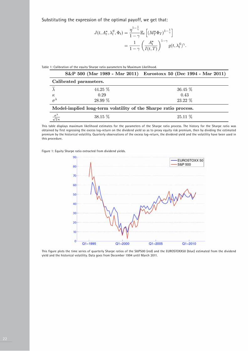
In contrast to those of the volatility process, parameters of the Sharpe ratio process appear in optimal portfolio weights (see Proposition 1), together with the current value of the Sharpe ratio. Their estimation is complicated by the fact that the Sharpe ratio is not observable. For the purpose of calibrating the model, we follow the literature (see e.g. campbell and Viceira (1999) and Munk et al. (2004)) in assuming that the equity risk premium follows a mean-reverting process and is an affine function of the dividend yield

(2.9)

We then estimate (2.9) by maximum likelihood, and extract the Sharpe ratio by dividing the implied risk premium by the volatility. Figure 1 displays the time series of implied Sharpe ratio for two indexes, Eurostoxx 50 and S&P 500. We retain as base case values for κ and the midpoints between the estimates for the two indexes, namely 35% and 40% respectively.

The anticipated inflation rate, π, is set to 1.58% per year, and the volatility of unexpected inflation to 0.57%. These values have been obtained by maximizing the likelihood of a Europeanconsumer Price Index over the period dec. 1994 to Mar. 2011.

We take the correlation between unexpected stock returns and innovations to the Sharpe ratio to be −1. This choice is empirically supported by various calibrations (see e.g. campbell and Viceira (1999) and Xia (2001)), and makes Sharpe ratio risk spanned by the stock itself. The correlation between unexpected stock returns and innovations to volatility is also set to a negative value ( − 76.7%) as in Ait-Sahalia and Kimmel (2007), to account for the fact that volatility tends to rise when stock returns go down. The correlation between the short-term rate and the price index is set to 13.80%, and the other correlations are set to zero. Finally, all mean-reverting parameters are initialized at their long-term mean.

2.4 Optimal Allocation in the General Settinghaving introduced the stochastic model for the economy, we can now obtain an analytical expression for expected utility-maximizing portfolio strategies.

2.4.1 Portfolio Strategies and ObjectiveLet wt denote the vector of weights allocated to the traded assets: nominal bond, stock and possibly the indexed bond. The budget constraint can be written as:

(2.10)

Throughout the paper, we let denote the investor’s constant Relative Risk Aversion (cRRA) utility function. In order to take liabilities into account, we assume that the investor has utility from his terminal nominal wealth rather than his terminal real wealth:

(2.11)

A similar problem has been solved by Brennan and Xia (2002), Munk et al. (2004) or Sangvinatsos and Wachter (2005), but in contrast with these papers, we allow for stochastic volatility and possibly unspanned Sharpe ratio risk.

2.4.2 A Four-Fund Separation ResultWe solve problem (2.11) using the martingale approach in incomplete markets of he and Pearson (1991). The solution is described in the next proposition. As is standard in the literature on dynamic portfolio choice, it is expressed as a linear combination of elementary portfolios (or blocks) that are independent from subjective characteristics (age and risk aversion).

Proposition 1 (Optimal Allocation In Possibly Incomplete Market) consider the optimization problem (2.11) subject to the budget condition (2.10). The optimal strategy is given by:

(2.12)

where:

• is the performance-seeking portfolio (PSP); and are its Sharpe ratio and volatility;

• is the liability-hedging portfolio (LhP), and is the beta of the indexed zero-coupon bond of maturity T with respect to the LhP;

• is the Sharpe ratio-hedging portfolio (SRhP), and is the beta of the Sharpe ratio with respect to the SRhP.

9

10 3 - In incomplete markets, Detemple and Rindisbacher (2010) price this zero-coupon under an investor-specific martingale measure known as the minimax martingale measure. In our decomposition, we price the zero-coupon under a different measure, such that the market price of inflation risk, λΦ, is constant. Were inflation risk spanned, these two prices would be equal.

The remainder of wealth is invested in cash (the fourth fund). The functions A1(·; γ), A2(·; γ) and A3(·; γ) are the solutions to a system of (coupled) ordinary differential equations (OdEs) given in Appendix A.1 with the initial conditions A1(0; γ) = A2(0; γ) = A3(0; γ) = 0.

Proof. See Appendix A.1.

If investment opportunities were constant, the optimal allocation of Proposition 1 would reduce to the PSP, which exhibits the highest Sharpe ratio by definition, and the cash, see (Merton, 1969). The composition of the PSP is continuously revised as a function of the Sharpe ratio and the volatility of the stock. The allocation to the PSP increases when the risk-return trade-off of this fund improves.

The second building block is the liability-hedging portfolio (LhP). It can be shown that it achieves the maximum correlation with an hypothetical indexed zero-coupon that pays off ΦT at date T, and which is the long-term risk-free asset for an investor concerned with the terminal real value of his portfolio. The maximum correlation of 1 is attained only if an indexed bond is traded. The allocation to this block is increasing in the risk aversion and in the beta of the hypothetical indexed bond with respect to the LhP.

The third building block, the SRhP, is the portfolio that hedges unexpected changes in the Sharpe ratio of the stock. The demand for this portfolio is non-zero, except in the following three situations: (i) the Sharpe ratio is constant (σλ = 0); (ii) the SRhP provides no hedge against Sharpe ratio risk (βSRhP = 0); (iii) the utility function of the investor is logarithmic. Moreover, the demand for the SRhP vanishes to zero as the investor gets closer to his horizon, since both A2 and A3

shrink to zero as the time-to-horizon goes to zero.

We note that there is no hedging demand against volatility risk, which is a special case of a more general property, stating that the agent will hedge only those state variables that impact the short-term interest rate r and the Sharpe ratio S (see detemple et al. (2003)). Overall, the above decomposition of the optimal portfolio is similar to the one introduced by detemple and Rindisbacher (2010).3

In Section 3, we will compare different strategies based on their expected utilities. The following proposition provides an expression for the expected utility associated with the optimal strategy, also known as indirect utility.

Proposition 2 (Maximal Expected Utility) The indirect utility function is:

Proof. See Appendix A.1.

2.4.3 differences Between Optimal Strategy and current Forms of TdFsIt is clear from Proposition 1 that the weights allocated to the bond and the stock are not only time-dependent, but also state-dependent, in contrast to the heuristic deterministic glide paths of existing life-cycle funds. In particular, the optimal allocation is a function of the Sharpe ratio and volatility of the stock. For this reason, it is very unlikely that the allocation to the stock will be a monotonic decreasing function of age. Only the allocation to the SRhP, which is fully invested in the stock if ρSλ = −1, shrinks to zero as the investor approaches retirement. This property comes from the fact that A2(0; γ) = A3(0; γ) = 0. But the optimal allocation to stocks also depends on the allocation to the PSP, which does not vanish even at maturity. For a young investor, the optimal allocation to the stock is larger than for an older one, but it is a function

of market conditions. In particular, it decreases when the stock market appears to be expensive in view of a low Sharpe ratio.4

Another important difference between the optimal strategy and current financial advice is that the weight of nominal bonds is not necessarily increasing over time. In fact, because the long-term risk-free asset is an indexed bond, nominal bonds do not play a particular role here. Indeed, they are risky in real terms, and are certainly not the best hedging instruments against inflation risk at maturity. A second issue with existing target-date funds is that they generally use constant-maturity nominal bonds. This approach is inconsistent with the optimal strategy, since as evidenced by the expression for the volatility vector of the indexed bond in (2.8), the optimal exposure to interest rate risk is decreasing over time, not constant.

2.5 Respecting Short-Term ConstraintsPrivate clients are also often concerned with drawdown: they do not want to lose more than a fraction δ of the maximum that their wealth has attained since the beginning of their investment.A drawdown constraint reads: , for all t, almost surely; (2.13)

where denotes the running maximum of wealth. Typical values for δ are 80%, 85% and 90%.

constraint (2.13) is satisfied if the portfolio is fully invested in cash.5 This observation suggests that the allocation to risky assets should shrink to zero as the risk budget shrinks to zero. An example of such allocations is:

(2.14)

where Add is the current wealth obtained by following the constrained strategy. Such strategies are of the same form as those considered in Grossman and Zhou (1993) and cvitanic and Karatzas (1995), who consider a slightly modified version of the drawdown constraint (2.13) by imposing that the discounted wealth stays above a fraction δ of its running maximum.

A related issue, that we do not discuss here, would be the imposition of a minimum level of wealth relative to liabilities at all dates (see deguest et al. (2011)).

3. Implementation ChallengesThe optimal strategy of Proposition 1 and the constrained strategy (2.14) are not directly implementable in practice, mainly for the following three reasons:• they assume continuous trading, while trading is possible only in discrete time;• they assume that short sales and leverage are permitted;• they assume a perfect knowledge of the current Sharpe ratio and volatility of the stock.

This assumption may be realistic as far as volatility is concerned, but is far too optimistic when it comes to the Sharpe ratio.

The first two issues are addressed in a standard way: it suffices to implement the strategy in discrete time and to resize the weights so as to rule out short positions and leverage. Addressing the non-observability of the Sharpe ratio is less straightforward. The solution that we propose below is based on a robust estimation of this quantity: rather than guessing its exact value, we pursue the more realistic objective of guessing whether it is low, medium or high.

11

4 - One can formally show that A3 is a positive increasing function of time-to-horizon, so that the weight allocated to the SRHP is always increasing in the Sharpe ratio, and the link between these two quantities loosens as time goes by.5 - Strictly speaking, the constraint can be violated even if the portfolio is entirely invested in cash, because negative interest rates are possible in the Vasicek model. Nevertheless such a situation is very unlikely, because the fact that δ < 1 allows for a slight decrease in the value of the bank account without it falling below the floor. Negative rates are problematic if they are persistent, but mean reversion towards a positive value avoids this undesirable effect.

12

By definition, taking into account the various implementation constraints will decrease the expected utility from terminal wealth. Our purpose in this section is to show that in fact the utility cost of these constraints, while being significant, is not dramatically high, and that it is anyway far lower than the utility cost of following a deterministic allocation scheme.

3.1 Description of Long-Term Investing StrategiesWe first describe the strategies used in the remainder of this paper. First, we assume that the investor has access to a perfect LhP, which is an inflation-linked bond expiring at time T. Second, we assume for simplicity mainly that the investor restricts his investment universe to stocks in the PSP. This assumption is motivated by the fact that (i) the PSP is built to maximize the Sharpe ratio over the investment universe, and would typicially involve a susbtantial investment in stocks, and (ii) the risky portfolio used in standard target date funds, which we use as benchmarks, is typically an equity index. These two assumptions imply that the investor does not invest in nominal bonds anymore since he reduces his investment vehicles to the perfect inflation-linked LhP and the stock index.

We represent the new portfolio strategies by a vector collecting the weights allocated to the stock and the perfect LhP. The weight allocated to cash is . We thus let . The LhP is fully invested in the indexed bond, so that , and under the assumption that ρSλ = −1, the SRhP is fully invested in the stock, so that . The beta of the Sharpe ratio with respect to the SRhP is thus .

Finally, in the absence of short-term constraints, we will consider strategies that retain the form of the optimal strategy in Proposition 1:

(3.1)

If drawdown constraints are imposed, we will consider strategies of the same form as in equation (2.14), namely:

with given by (3.1).

The vectors of weights and define a family of strategies to which we will refer as LTIB (Long-Term Investing Benchmarks). These strategies are parameterized by three subjective parameters: the initial time-to-horizon T, the relative risk aversion γ and the maximum acceptable drawdown 1 − δ. The parameter T is observable, and in the subsequent numerical results, we take it equal to 20 years unless otherwise stated. The risk aversion γ is not observable, so we will calibrate it in such a way that the average allocation to equity over the 20-year life of the fund is equal to a target of 10%, 20% or 30%. The three corresponding sub-families of LTIB will be referred to as defensive (γ = 55 leading to an average stock weight of 9.95%), moderate (γ = 23 leading to an average stock weight of 19.90%) and aggressive (γ = 12 leading to an average stock weight of 30.76%), respectively. It should be noted that the allocation to the stock at a given date can be substantially higher than the average allocation, especially at the beginning of the period. Finally, the values for the maximum drawdown 1 − δ will be discussed in Section 4.

3.2 Monetary Utility LossesIn this section, we present a measure of performance called Monetary Utility Losses (MUL) which quantifies the loss of expected utility of implementing a sub-optimal strategy as opposed to the optimal strategy.

Let denote the terminal wealth achieved by investing A0 at time 0 in some sub-optimal strategy. We also denote with the terminal wealth generated by program (2.11). The MUL is defined as the additional capital x that needs to be invested at time 0 in some suboptimal strategy in order to make its expected utility equal to the one generated by the optimal strategy:

(3.2)

We now show that an explicit expression for x can be obtained, when the sub-optimal strategy is rebalanced at the discrete dates , and that the weights for 1 ≤ i ≤ n do not depend on current wealth. We define as the vector of realized returns on risky assets (stock index and indexed zero-coupon bond) over the period [ti, ti +1], and as the realized return on the bank account. Over each time interval [ti, ti +1], the portfolio is left buy-and-hold, hence the wealth evolves as:

With the definition , this expression leads to:

hence is proportional to the initial capital, A0. In particular, we have:

Substituting this expression into (3.2) and using Proposition 2, we obtain:

hence, in order to practically compute the MUL, it suffices to estimate the expected utility of the sub-optimal strategy. We do this by simulating 10,000 outcomes for the payoff of this strategy for an initial wealth of $1.6

3.3 Discrete-Time Implementation of Long-Term Investing StrategiesThe optimal strategy (2.12) was derived under the assumption that trading takes place in continuous time. In practice, however, continuous trading is impossible because it would incur prohibitively high transaction costs. Therefore, all the strategies that we subsequently test are implemented at discrete dates with a constant time-step Δt = ti+1 − ti. We choose a quarterly rebalancing period.

Table 3 displays the Monetary Utility Losses of discretized sub-optimal strategies, implemented with a quarterly rebalancing frequency, and denoted LTIB(∞, ∞) (this notation will be explained below). This utility cost includes the sub-optimality coming from the approximation of the PSP by a portfolio of stock only, and from the discrete rebalancing. In order to assess the economic significance of these losses, we compare them to those incurred by strategies similar to currently available target-date funds. These strategies, which we shall refer to simply as TdFs, are rebalanced on an annual basis. At date 0, they allocate the weight wi to stocks and 1 − wi to constant-maturity bonds, and at the beginning of year T − 1, they allocate wf to stocks. At the beginning of year j, the weight of stocks is:

136 - In our Monte-Carlo simulations, we imposed bounds of = 10% and = 40% at each date to the volatility, and bounds of = 25% and = 75% to the Sharpe ratio.

14

We will consider a TdF that decreases the allocation to stocks from 60% to 20% in 20 years, and a more aggressive one, that goes from 90% to 60%. Table 3 shows that for all investor’s risk profiles, implementing a TdF causes a much higher utility loss than implementing a LTIB strategy. In other words, LTIB strategies are closer to the optimal strategy in terms of expected utility. This result confirms the findings of cairns et al. (2006), who show that stochastic lifestyling strategies outperform deterministic strategies.

3.4 Imposing Short-Sale Constraints on Asset HoldingsSince no short-sales constraints have been imposed ex-ante to the weights of the optimal strategy, there is no reason why all of them would fall between 0 and 1. however, short-selling is often not desired by practitioners of the retail industry, or even prohibited by regulators. Since there is no known closed-form expression for the optimal strategy in (2.11) with short-sales and leverage constraints, we resize the unconstrained weights in order to ensure that they are nonnegative and that their sum does not exceed 1:

where (x)+ denotes max(0, x). The weight allocated to cash is

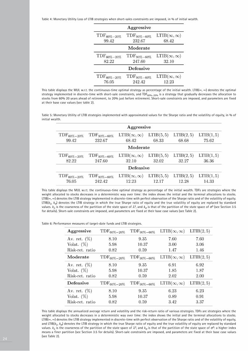
We compute in Table 4 the loss of utility that follows from the imposition of these constraints, and compare it to the MUL of the deterministic TdFs. Note that by construction, the two TdF strategies do not involve short positions, which implies that their MULs remain unchanged. On the other hand, we observe that the MUL of the LTIB(∞, ∞) increases when we impose the short-sale constraints. Nonetheless, it remains far below the MULs of the deterministic strategies, which shows that LTIB strategies remain superior even after short-sale constraints have been taken into account.

3.5 Introducing a Discrete Partition of the Set Market ConditionsSince the equity Sharpe ratio λS and the equity volatility σS are not directly observable, we will rely on estimation methods in order to estimate these two processes at all time. Following Martellini and Milhau (2010), we propose to discretize the state spaces of these two processes, using a finer grid mesh for the volatility because it is known that the Sharpe ratio is much harder to estimate than the volatility (see Merton (1980)). Since this discretization introduces a loss of optimality, we will quantify its impact in terms of utility loss through the computation of MULs.

The crudest possible partition of market conditions would involve replacing all realizations of λS by a constant, and all those of S by another constant. We choose these constants to be the midpoints between the lower bound and the upper bounds imposed during the simulations.

hence, at the first level of partition, all realizations of λS are replaced by , and all realizations of σS by .

The second partitioning level of the set of market conditions involves distinguishing betweenhigh, moderate and low risk premium levels, and therefore contains three buckets:

Each realization of λS is then replaced by one of the “standard values” , and . Moregenerally, one can construct partitions of any level k, such that for k ≥ 1. The kth partitioning level has 2k−1 + 1 standard values. In what follows, we will denote with kλ the index of the partition of the state space of values of σS, and kσ the index of the partition for the values of σS. Since the estimation of the Sharpe ratio is known to be difficult, we will work with very low partitioning levels (kλ = 1 or 2). On the other hand, the estimation of the volatility is easier, so we can consider very high values of kσ (possibly 5; which corresponds to 17 standard values). The strategy using kλ partitioning levels for S, and k partitioning levels for λS will be denoted by LTIB(kλ, kσ) in the sequel. For kλ = 0 and kσ = ∞, the true values of the Sharpe ratio and of the volatility are used in the expression of the strategy, so the strategy LTIB(∞, ∞) differs from the optimal strategy only by the discrete-time implementation and the imposition of short-sale constraints.

Table 5 summarizes the various MULs for the three risk aversions considered and various LTIB strategies. It is interesting to note that the marginal utility loss that occurs when one chooses strategy LTIB(2, 5) instead of LTIB(∞, ∞) is very low, almost negligible. This encourages us to estimate only three levels of equity Sharpe ratio in order to implement our LTIB strategies, since going beyond would not significantly improve expected utility. This seems to be feasible in practice since we only need to be able to say if the Sharpe ratio is high, medium or low.

3.6 Assessing Long-Term Performance of Life-Cycle StrategiesA natural indicator of long-term performance is the annualized expected log-real return on the strategy:

As explained in Section 3.2, the terminal value of the LTIB strategy is proportional to the initial capital invested, so that . Moreover, Φ0 is normalized to 1. hence the expected return, and more generally any indicator based on the real log-return, is independent from A0. Nonetheless, looking only at this quantity to assess the performances of a fund is very reductive since it completely disregards risk, both on the long run and on the short run.

A standard measure of long-term risk is the annualized standard deviation of the real log-return: In order to aggregate the risk and return dimensions, we compute a risk-return ratio, which measures the risk-adjusted excess expected return of the strategy:

where denotes the annualized expected log- real return on cash.

In Table 6, we compute all these quantities for different funds (our LTIB strategies and the two target-date funds). It turns out that the risk-return ratios of LTIB strategies are much higher than those of the deterministic strategies, which shows that LTIB strategies dominate TdFs not only in terms of expected utility (which was the bottom line of tables 3 through 5), but also in terms of risk-return ratio.

4. Communication ChallengesThe results we obtained in Section 3 confirm that existing forms of allocation strategies, such as those represented by balanced funds or target date funds, are strongly dominated by strategies

15

16

that are good approximations to truly optimal strategies and that satisfy realistic implementation constraints. In this section, we argue that deterministic strategies are also not consistent with the respect of private and retail clients’ long-term objectives and short-term constraints, while these objectives and constraints can be satisfactorily addressed by LTIB strategies. This approach to private or retail wealth management brings along an entirely different mode of relationship with the client. It is not based on an analysis expressed in terms of comparison of performances, but instead on an analysis expressed in terms of an assessment of the client’s ability to meet their various objectives and constraints. Therefore, this section will specifically emphasize on the four following aspects:• Performance Assessment;• Budgeting risk- and loss- aversion;• Impact of time-horizon;• Impact of liabilities.

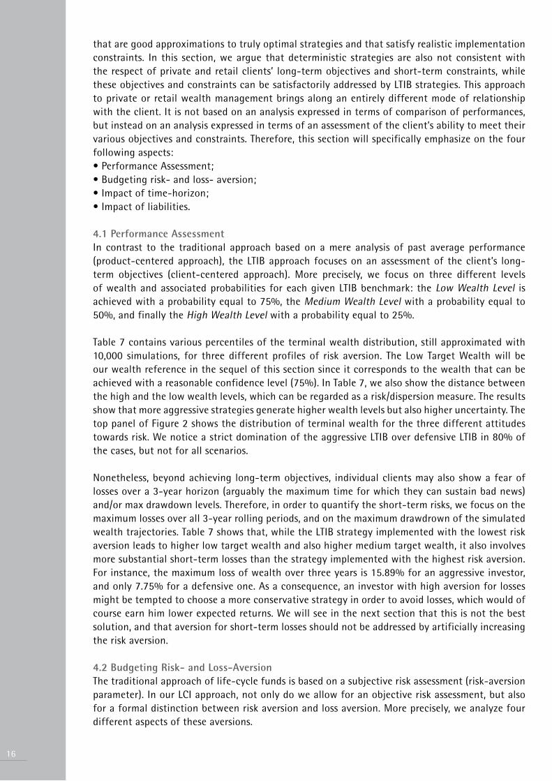
4.1 Performance AssessmentIn contrast to the traditional approach based on a mere analysis of past average performance (product-centered approach), the LTIB approach focuses on an assessment of the client’s long-term objectives (client-centered approach). More precisely, we focus on three different levels of wealth and associated probabilities for each given LTIB benchmark: the Low Wealth Level is achieved with a probability equal to 75%, the Medium Wealth Level with a probability equal to 50%, and finally the high Wealth Level with a probability equal to 25%.

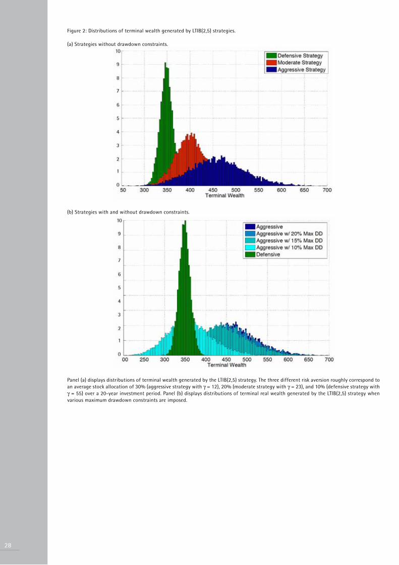
Table 7 contains various percentiles of the terminal wealth distribution, still approximated with 10,000 simulations, for three different profiles of risk aversion. The Low Target Wealth will be our wealth reference in the sequel of this section since it corresponds to the wealth that can be achieved with a reasonable confidence level (75%). In Table 7, we also show the distance between the high and the low wealth levels, which can be regarded as a risk/dispersion measure. The results show that more aggressive strategies generate higher wealth levels but also higher uncertainty. The top panel of Figure 2 shows the distribution of terminal wealth for the three different attitudes towards risk. We notice a strict domination of the aggressive LTIB over defensive LTIB in 80% of the cases, but not for all scenarios.

Nonetheless, beyond achieving long-term objectives, individual clients may also show a fear of losses over a 3-year horizon (arguably the maximum time for which they can sustain bad news) and/or max drawdown levels. Therefore, in order to quantify the short-term risks, we focus on the maximum losses over all 3-year rolling periods, and on the maximum drawdrown of the simulated wealth trajectories. Table 7 shows that, while the LTIB strategy implemented with the lowest risk aversion leads to higher low target wealth and also higher medium target wealth, it also involves more substantial short-term losses than the strategy implemented with the highest risk aversion. For instance, the maximum loss of wealth over three years is 15.89% for an aggressive investor, and only 7.75% for a defensive one. As a consequence, an investor with high aversion for losses might be tempted to choose a more conservative strategy in order to avoid losses, which would of course earn him lower expected returns. We will see in the next section that this is not the best solution, and that aversion for short-term losses should not be addressed by artificially increasing the risk aversion.

4.2 Budgeting Risk- and Loss-AversionThe traditional approach of life-cycle funds is based on a subjective risk assessment (risk-aversion parameter). In our LcI approach, not only do we allow for an objective risk assessment, but also for a formal distinction between risk aversion and loss aversion. More precisely, we analyze four different aspects of these aversions.

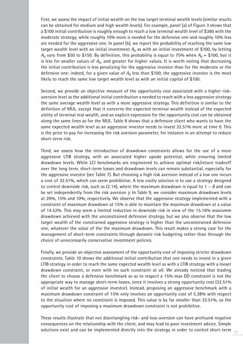
First, we assess the impact of initial wealth on the low target terminal wealth levels (similar results can be obtained for medium and high wealth levels). For example, panel (a) of Figure 3 shows that a $100 initial contribution is roughly enough to reach a low terminal wealth level of $380 with the moderate strategy, while roughly 10% more is needed for the defensive one and roughly 10% less are needed for the aggressive one. In panel (b), we report the probability of reaching the same low target wealth level with an initial investment A0 as with an initial investment of $100, by letting A0 vary from $50 to $150. By definition, this probability is equal to 75% when A0 = $100, but it is less for smaller values of A0, and greater for higher values. It is worth noting that decreasing the initial contribution is less penalizing for the aggressive investor than for the moderate or the defensive one: indeed, for a given value of A0 less than $100, the aggressive investor is the most likely to reach the same low target wealth level as with an initial capital of $100.

Second, we provide an objective measure of the opportunity cost associated with a higher risk-aversion level as the additional initial contribution x needed to reach with a less aggressive strategy the same average wealth level as with a more aggressive strategy. This definition is similar to the definition of MUL, except that it concerns the expected terminal wealth instead of the expected utility of terminal real wealth, and an explicit expression for the opportunity cost can be obtained along the same lines as for the MUL. Table 8 shows that a defensive client who wants to have the same expected wealth level as an aggressive investor needs to invest 32.51% more at time 0. This is the price to pay for increasing the risk aversion parameter, for instance in an attempt to reduce short-term risk.

Third, we assess how the introduction of drawdown constraints allows for the use of a more aggressive LTIB strategy, with an associated higher upside potential, while ensuring limited drawdown levels. While LcI benchmarks are engineered to achieve optimal risk/return tradeoff over the long term, short-term losses and drawdown levels can remain substantial, especially for the aggressive investor (see Table 7). But choosing a high risk aversion instead of a low one incurs a cost of 32.51%, which can seem prohibitive. A less costly solution is to use a strategy designed to control downside risk, such as (2.14), where the maximum drawdown is equal to 1 − δ and can be set independently from the risk aversion γ. In Table 9, we consider maximum drawdown levels at 20%, 15% and 10%, respectively. We observe that the aggressive strategy implemented with a constraint of maximum drawdown at 15% is able to maintain the maximum drawdown at a value of 14.52%. This may seem a limited reduction in downside risk in view of the 15.16% maxiumm drawdown achieved with the unconstrained defensive strategy, but we also observe that the low target wealth of the constrained aggressive strategy is higher than the unconstrained defensive one, whatever the value of the the maximum drawdown. This result makes a strong case for the management of short-term constraints through dynamic risk budgeting rather than through the choice of unnecessarily conservative investment policies.

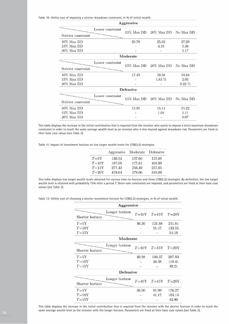
Finally, we provide an objective assessment of the opportunity cost of imposing stricter drawdown constraints. Table 10 shows the additional initial contribution that one needs to invest in a given LTIB strategy in order to reach the same expected wealth level as with a LTIB strategy with a looser drawdown constraint, or even with no such constraint at all. We already noticed that leading the client to choose a defensive benchmark so as to respect a 15% max dd constraint is not the appropriate way to manage short-term losses, since it involves a strong opportunity cost (32.51% of initial wealth for an aggressive investor). Instead, proposing an aggressive benchmark with a maximum drawdown constraint of 15% only involves an opportunity cost of 5.38% with respect to the situation where no constraint is imposed. This value is by far smaller than 32.51%, so the opportunity cost of imposing a maximum drawdown constraint is not prohibitive.

These results illustrate that not disentangling risk- and loss-aversion can have profound negative consequences on the relationship with the client, and may lead to poor investment advice. Simple solutions exist and can be implemented directly into the strategy in order to control short-term 17

18

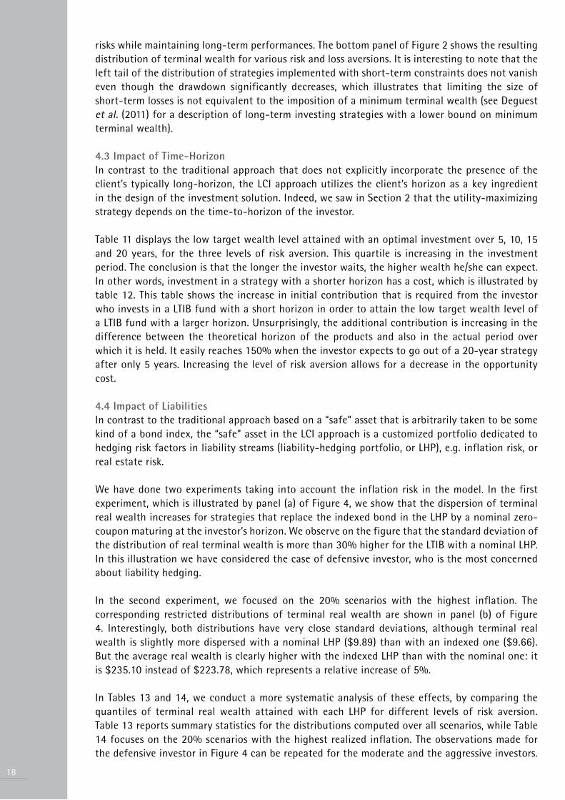
risks while maintaining long-term performances. The bottom panel of Figure 2 shows the resulting distribution of terminal wealth for various risk and loss aversions. It is interesting to note that the left tail of the distribution of strategies implemented with short-term constraints does not vanish even though the drawdown significantly decreases, which illustrates that limiting the size of short-term losses is not equivalent to the imposition of a minimum terminal wealth (see deguest et al. (2011) for a description of long-term investing strategies with a lower bound on minimum terminal wealth).

4.3 Impact of Time-HorizonIn contrast to the traditional approach that does not explicitly incorporate the presence of the client’s typically long-horizon, the LcI approach utilizes the client’s horizon as a key ingredient in the design of the investment solution. Indeed, we saw in Section 2 that the utility-maximizingstrategy depends on the time-to-horizon of the investor.

Table 11 displays the low target wealth level attained with an optimal investment over 5, 10, 15 and 20 years, for the three levels of risk aversion. This quartile is increasing in the investment period. The conclusion is that the longer the investor waits, the higher wealth he/she can expect. In other words, investment in a strategy with a shorter horizon has a cost, which is illustrated by table 12. This table shows the increase in initial contribution that is required from the investor who invests in a LTIB fund with a short horizon in order to attain the low target wealth level of a LTIB fund with a larger horizon. Unsurprisingly, the additional contribution is increasing in the difference between the theoretical horizon of the products and also in the actual period over which it is held. It easily reaches 150% when the investor expects to go out of a 20-year strategy after only 5 years. Increasing the level of risk aversion allows for a decrease in the opportunity cost.

4.4 Impact of LiabilitiesIn contrast to the traditional approach based on a “safe” asset that is arbitrarily taken to be some kind of a bond index, the “safe” asset in the LcI approach is a customized portfolio dedicated to hedging risk factors in liability streams (liability-hedging portfolio, or LhP), e.g. inflation risk, or real estate risk.

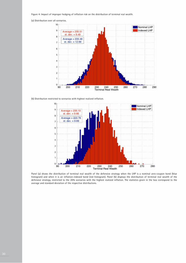
We have done two experiments taking into account the inflation risk in the model. In the first experiment, which is illustrated by panel (a) of Figure 4, we show that the dispersion of terminal real wealth increases for strategies that replace the indexed bond in the LhP by a nominal zero-coupon maturing at the investor’s horizon. We observe on the figure that the standard deviation of the distribution of real terminal wealth is more than 30% higher for the LTIB with a nominal LhP. In this illustration we have considered the case of defensive investor, who is the most concerned about liability hedging.

In the second experiment, we focused on the 20% scenarios with the highest inflation. The corresponding restricted distributions of terminal real wealth are shown in panel (b) of Figure 4. Interestingly, both distributions have very close standard deviations, although terminal real wealth is slightly more dispersed with a nominal LhP ($9.89) than with an indexed one ($9.66). But the average real wealth is clearly higher with the indexed LhP than with the nominal one: it is $235.10 instead of $223.78, which represents a relative increase of 5%.

In Tables 13 and 14, we conduct a more systematic analysis of these effects, by comparing the quantiles of terminal real wealth attained with each LhP for different levels of risk aversion. Table 13 reports summary statistics for the distributions computed over all scenarios, while Table 14 focuses on the 20% scenarios with the highest realized inflation. The observations made for the defensive investor in Figure 4 can be repeated for the moderate and the aggressive investors.

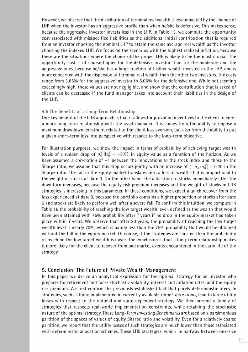
however, we observe that the distribution of terminal real wealth is less impacted by the change of LhP when the investor has an aggressive profile than when he/she is defensive. This makes sense, because the aggressive investor invests less in the LhP. In Table 15, we compute the opportunity cost associated with misspecified liabilities as the additional initial contribution that is required from an investor choosing the nominal LhP to attain the same average real wealth as the investor choosing the indexed LhP. We focus on the scenarios with the highest realized inflation, because these are the situations where the choice of the proper LhP is likely to be the most crucial. The opportunity cost is of course higher for the defensive investor than for the moderate and the aggressive ones, because he/she has a large fraction of his/her wealth invested in the LhP, and is more concerned with the dispersion of terminal real wealth than the other two investors. The costs range from 3.85% for the aggressive investor to 5.06% for the defensive one. While not seeming exceedingly high, these values are not negligible, and show that the contribution that is asked of clients can be decreased if the fund manager takes into account their liabilities in the design of the LhP.

4.5 The Benefits of a Long-Term RelationshipOne key benefit of the LTIB approach is that it allows for providing incentives to the client to enter a more long-term relationship with the asset manager. This comes from the ability to impose a maximum drawdown constraint related to the client loss aversion, but also from the ability to put a given short-term loss into perspective with respect to the long-term objective.

For illustration purposes, we show the impact in terms of probability of achieving target wealth levels of a sudden drop of in equity value as a function of the horizon. As we have assumed a correlation of −1 between the innovations to the stock index and those to the Sharpe ratio, we assume that this drop occurs jointly with an increase of in the Sharpe ratio. The fall in the equity market translates into a loss of wealth that is proportional to the weight of stocks at date 0. On the other hand, the allocation to stocks immediately after the downturn increases, because the equity risk premium increases and the weight of stocks in LTIB strategies is increasing in this parameter. In these conditions, we expect a quick recover from the loss experienced at date 0, because the portfolio contains a higher proportion of stocks after date 0 and stocks are likely to perform well after a severe fall. To confirm this intuition, we compute in Table 16 the probability of reaching the low target wealth level, defined as the wealth that would have been attained with 75% probability after T years if no drop in the equity market had taken place within T years. We observe that after 20 years, the probability of reaching the low target wealth level is nearly 70%, which is hardly less than the 75% probability that would be obtained without the fall in the equity market. Of course, if the strategies are shorter, then the probability of reaching the low target wealth is lower. The conclusion is that a long-term relationship makes it more likely for the client to recover from bad market events encountered in the early life of the strategy.

5. Conclusion: The Future of Private Wealth ManagementIn this paper we derive an analytical expression for the optimal strategy for an investor who prepares for retirement and faces stochastic volatility, interest and inflation rates, and the equity risk premium. We first confirm the previously established fact that purely deterministic lifecycle strategies, such as those implemented in currently available target-date funds, lead to large utility losses with respect to the optimal and state-dependent strategy. We then present a family of strategies that respects real-world implementation constraints, while retaining the stochastic nature of the optimal strategy. These Long-Term Investing Benchmarks are based on a parsimonious partition of the spaces of values of equity Sharpe ratio and volatility. Even for a relatively coarse partition, we report that the utility losses of such strategies are much lower than those associated with deterministic allocation schemes. These LTIB strategies, which lie halfway between one-size

19

20

fits-all solutions and do-it-yourself approaches, are thus very good approximations of the truly optimal allocation strategy. They also allow to meet the client’s short-term constraints, which are simply not taken into account by existing target-date funds. Finally, they imply an entirely new mode of relationship with the clients, based on a focus on the client’s needs, as opposed to a focus on a particular product’s performance in a particular sample period.

A. Proofs of the Main PropositionsA.1 Proof of Propositions 1 and 2As shown by he and Pearson (1991), program (2.11) is equivalent to the following “static” program:

(A.1)

where M* is the “minimax pricing kernel”. The optimal payoff is obtained by writing the first-order optimality condition with respect to the terminal wealth:

The time t value of the optimal portfolio is then obtained by discounting the optimal payoff with the minimax pricing kernel:

(A.2)

In what follows, we let:

Since the process M*A* is a martingale, its drift term must be zero. Applying Ito’s lemma, we can write this condition as:

(A.3)

Moreover, the volatility vector of A* must be spanned by the columns of the unit volatility matrix of traded risks . defining as the identity matrix matrix, and as the matrix of the residual of the orthogonal projection onto the columns of , we have:

Since and , this is equivalent to:

Substituting this back into (A.3), we obtain that g must solve the following partial differential equation (PdE):

(A.4)

where we have decomposed as and and are canonical unit vectors (note that is a canonical vector if the indexed bond is traded, and is zero otherwise). The terminal condition is g(T, λ) = 1.

It remains to solve (A.4). Let us try a solution of the form:

If we substitute back the first- and second-order partial derivatives of g into the right side of (A.4), we obtain a linear combination of 1, λ and λ2 with deterministically time-dependent coefficients. This linear combination must be zero for each value of λ, hence the three time-dependent coefficients must be zero at all dates. Writing each of these conditions leads to the following system of three coupled ordinary differential equations (OdEs):

(A.5)

In these equations, we have set

The optimal portfolio policy is given by:

where is the volatility vector of A*. Applying Ito’s lemma to (A.2), we get that:

We then define the four building blocks as in the proposition, and we let and denote the volatility and the Sharpe ratio of the PSP, denote the beta of the indexed bond of maturity T with respect to the LhP and denote the beta of the Sharpe ratio of the stock with respect to the SRhP. These definitions imply that:

The indirect utility function is defined by:

21

22

Substituting the expression of the optimal payoff, we get that:

Table 1: calibration of the equity Sharpe ratio parameters by Maximum Likelihood.

This table displays maximum likelihood estimates for the parameters of the Sharpe ratio process. The history for the Sharpe ratio was obtained by first regressing the excess log-return on the dividend yield so as to proxy equity risk premium, then by dividing the estimated premium by the historical volatility. Quarterly observations of the excess log-return, the dividend yield and the volatility have been used in this procedure.

Figure 1: Equity Sharpe ratio extracted from dividend yields.

This figure plots the time series of quarterly Sharpe ratios of the S&P500 (red) and the EUROSTOXX50 (blue) estimated from the dividend yield and the historical volatility. data goes from december 1994 until March 2011.

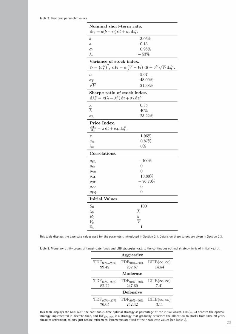
Table 2: Base case parameter values.

This table displays the base case values used for the parameters introduced in Section 2.1. details on these values are given in Section 2.3.

Table 3: Monetary Utility Losses of target-date funds and LTIB strategies w.r.t. to the continuous optimal strategy, in % of initial wealth.

This table displays the MUL w.r.t. the continuous-time optimal strategy as percentage of the initial wealth. LTIB(∞, ∞) denotes the optimal strategy implemented in discrete-time, and TdF60%−20% is a strategy that gradually decreases the allocation to stocks from 60% 20 years ahead of retirement, to 20% just before retirement. Parameters are fixed at their base case values (see Table 2).

23

24

Table 4: Monetary Utility Loss of LTIB strategies when short-sales constraints are imposed, in % of initial wealth.

This table displays the MUL w.r.t. the continuous-time optimal strategy as percentage of the initial wealth. LTIB(∞, ∞) denotes the optimal strategy implemented in discrete-time with short-sale constraints, and TdF60%−20% is a strategy that gradually decreases the allocation to stocks from 60% 20 years ahead of retirement, to 20% just before retirement. Short-sale constraints are imposed, and parameters are fixed at their base case values (see table 2).

Table 5: Monetary Utility of LTIB strategies implemented with approximated values for the Sharpe ratio and the volatility of equity, in % of initial wealth.

This table displays the MUL w.r.t. the continuous-time optimal strategy as percentage of the initial wealth. TdFs are strategies where the weight allocated to stocks decreases in a deterministic way over time: the index shows the initial and the terminal allocations to stocks. LTIB(∞, ∞) denotes the LTIB strategy implemented in discrete-time with perfect observation of the Sharpe ratio and of the volatility of equity. LTIB(kλ, kσ) denotes the LTIB strategy in which the true Sharpe ratio of equity and the true volatility of equity are replaced by standard values. kλ is the coarseness of the partition of the state space of λS, and kσ is that of the partition of the state space of σS (see Section 3.5 for details). Short-sale constraints are imposed, and parameters are fixed at their base case values (see Table 2).

Table 6: Performance measures of target-date funds and LTIB strategies.

This table displays the annualized average return and volatility and the risk-return ratio of various strategies. TdFs are strategies where the weight allocated to stocks decreases in a deterministic way over time: the index shows the initial and the terminal allocations to stocks. LTIB(∞, ∞) denotes the LTIB strategy implemented in discrete-time with perfect observation of the Sharpe ratio and of the volatility of equity, and LTIB(kλ, kσ) denotes the LTIB strategy in which the true Sharpe ratio of equity and the true volatility of equity are replaced by standard values. kλ is the coarseness of the partition of the state space of λS, and kσ is that of the partition of the state space of σS: a higher index means a finer partition (see Section 3.5 for details). Short-sale constraints are imposed, and parameters are fixed at their base case values (see Table 2).

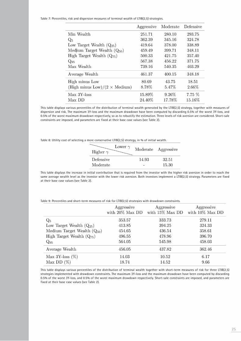
Table 7: Percentiles, risk and dispersion measures of terminal wealth of LTIB(2,5) strategies.

This table displays various percentiles of the distribution of terminal wealth generated by the LTIB(2,5) strategy, together with measures of dispersion and risk. The maximum 3Y-loss and the maximum drawdown have been computed by discarding 0.5% of the worst 3Y-loss, and 0.5% of the worst maximum drawdown respectively, so as to robustify the estimation. Three levels of risk aversion are considered. Short-sale constraints are imposed, and parameters are fixed at their base case values (see Table 2).

Table 8: Utility cost of selecting a more conservative LTIB(2,5) strategy, in % of initial wealth.

This table displays the increase in initial contribution that is required from the investor with the higher risk aversion in order to reach the same average wealth level as the investor with the lower risk aversion. Both investors implement a LTIB(2,5) strategy. Parameters are fixed at their base case values (see Table 2).

Table 9: Percentiles and short-term measures of risk for LTIB(2,5) strategies with drawdown constraints.

This table displays various percentiles of the distribution of terminal wealth together with short-term measures of risk for three LTIB(2,5) strategies implemented with drawdown constraints. The maximum 3Y-loss and the maximum drawdown have been computed by discarding 0.5% of the worst 3Y-loss, and 0.5% of the worst maximum drawdown respectively. Short-sale constraints are imposed, and parameters are fixed at their base case values (see Table 2).

25

26

Table 10: Utility cost of imposing a stricter drawdown constraint, in % of initial wealth.

This table displays the increase in the initial contribution that is required from the investor who wants to impose a strict maximum drawdown constraint in order to reach the same average wealth level as an investor who is less insured against drawdown risk. Parameters are fixed at their base case values (see Table 2).

Table 11: Impact of investment horizon on low target wealth levels for LTIB(2,5) strategies.

This table displays low target wealth levels obtained for various time-to-horizon and three LTIB(2,5) strategies. By definition, the low target wealth level is attained with probability 75% after a period T. Short-sale constraints are imposed, and parameters are fixed at their base case values (see Table 2).

Table 12: Utility cost of choosing a shorter investment horizon for LTIB(2,5) strategies, in % of initial wealth.

This table displays the increase in the initial contribution that is required from the investor with the shorter horizon in order to reach the same average wealth level as the investor with the longer horizon. Parameters are fixed at their base case values (see Table 2).

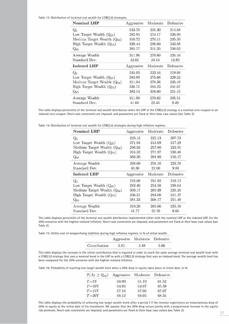
Table 13: distribution of terminal real wealth for LTIB(2,5) strategies.

This table displays percentiles of the terminal real wealth distribution when the LhP of the LTIB(2,5) strategy is a nominal zero-coupon or an indexed zero-coupon. Short-sale constraints are imposed, and parameters are fixed at their base case values (see Table 2).

Table 14: distribution of terminal real wealth for LTIB(2,5) strategies during high inflation regimes.

This table displays percentiles of the terminal real wealth distribution implemented either with the nominal LhP or the indexed LhP, for the 20% scenarios with the highest realized inflation. Short-sale constraints are imposed, and parameters are fixed at their base case values (see Table 2).

Table 15: Utility cost of misspecifying liabilities during high inflation regimes, in % of initial wealth.

This table displays the increase in the initial contribution that is required in order to reach the same average terminal real wealth level with a LTIB(2,5) strategy that uses a nominal bond in the LhP as with a LTIB(2,5) strategy that uses an indexed bond. The average wealth level has been computed for the 20% scenarios with the highest realized inflation.

Table 16: Probability of reaching low target wealth level when a 20% drop in equity takes place at initial date, in %.

This table displays the probability of achieving low target wealth levels after a period T if the investor experiences an instantaneous drop of 20% in equity at the initial date of his investment. We assume that the 20% drop occurs jointly with a proportional increase in the equity risk premium. Short-sale constraints are imposed, and parameters are fixed at their base case values (see Table 2).

27

28

Figure 2: distributions of terminal wealth generated by LTIB(2,5) strategies.

(a) Strategies without drawdown constraints.

(b) Strategies with and without drawdown constraints.

Panel (a) displays distributions of terminal wealth generated by the LTIB(2,5) strategy. The three different risk aversion roughly correspond to an average stock allocation of 30% (aggressive strategy with γ = 12), 20% (moderate strategy with γ = 23), and 10% (defensive strategy with γ = 55) over a 20-year investment period. Panel (b) displays distributions of terminal real wealth generated by the LTIB(2,5) strategy when various maximum drawdown constraints are imposed.

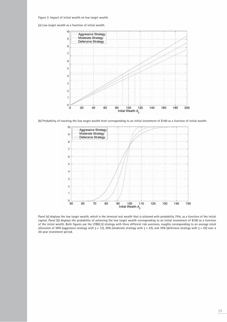
Figure 3: Impact of initial wealth on low target wealth.

(a) Low target wealth as a function of initial wealth.

(b) Probability of reaching the low target wealth level corresponding to an initial investment of $100 as a function of initial wealth.

Panel (a) displays the low target wealth, which is the terminal real wealth that is attained with probability 75%, as a function of the initial capital. Panel (b) displays the probability of achieving the low target wealth corresponding to an initial investment of $100 as a function of the initial wealth. Both figures use the LTIB(2,5) strategy with three different risk aversions, roughly corresponding to an average stock allocation of 30% (aggressive strategy with γ = 12), 20% (moderate strategy with γ = 23), and 10% (defensive strategy with γ = 55) over a 20-year investment period.

29

30

Figure 4: Impact of improper hedging of inflation risk on the distribution of terminal real wealth.

(a) distribution over all scenarios.

(b) distribution restricted to scenarios with highest realized inflation.

Panel (a) shows the distribution of terminal real wealth of the defensive strategy when the LhP is a nominal zero-coupon bond (blue histogram) and when it is an inflation-indexed bond (red histogram). Panel (b) displays the distribution of terminal real wealth of the defensive strategy, restricted to the 20% scenarios with the highest realized inflation. The statistics given in the box correspond to the average and standard deviation of the respective distributions.

References• Ait-Sahalia, Y. and R. Kimmel (2007). Maximum Likelihood Estimation of Stochastic Volatility Models. Journal of Financial Economics 83 (2), 413–452.

• Amenc, N., S. Focardi, F. Goltz, d. Schröder, and L. Tang (2010). Edhec-risk european private wealth management survey. EdhEc-Risk Institute Publication. Available at http://www.edhec-risk.com/edhec publications/all publications/RISKReview.2010-11-30.5229/attachments/EdhEc-Risk European Private Wealth Management Survey.pdf.

• Amenc, N., L. Martellini, V. Milhau, and V. Ziemann (2009). Asset-liability management in private wealth management. Journal of Portfolio Management 36 (1), 100–120.

• Bajeux-Besnainou, I., J. Jordan, and R. Portait (2003). dynamic Asset Allocation for Stocks, Bonds, and cash. The Journal of Business 76 (2), 263–287.

• Basu, A. and A. Brisbane (2009). Towards a dynamic asset allocation framework for target retirement funds: Getting rid of the dogma in lifecycle investing. Working Paper.

• Basu, A. and M. drew (2009). Portfolio size effect in retirement accounts: What does it imply for lifecycle asset allocation funds? The Journal of Portfolio Management 35 (3), 61–72.

• Benzoni, L., P. collin-dufresne, and R. Goldstein (2007). Portfolio choice over the life-cycle when the stock and labor markets are cointegrated. Journal of Finance 62 (5), 2123–2167.

• Bodie, Z., J. detemple, and M. Rindisbacher (2009). Life cycle finance and the design of pension plans. 1, 249–286. Annual Review of Financial Economics.

• Brennan, M., E. Schwartz, and R. Lagnado (1997). Strategic asset allocation. Journal of Economic dynamics and control 21 (8-9), 1377–1403.

• Brennan, M. and Y. Xia (2002). dynamic asset allocation under inflation. Journal of Finance 57 (3), 1201–1238.

• cairns, A., d. Blake, and K. dowd (2006). Stochastic lifestyling: Optimal dynamic asset allocation for defined contribution pension plans. Journal of Economic dynamics and control 30 (5), 843–877.

• campbell, J., Y. chan, and L. Viceira (2003). A multivariate model of strategic asset allocation. Journal of Financial Economics 67 (1), 41–80.

• campbell, J. and L. Viceira (1999). consumption and portfolio decisions when expected returns are time varying. Quarterly Journal of Economics 114 (2), 433–495.

• campbell, J. and L. Viceira (2005). The term structure of the risk-return trade-off. Financial Analysts Journal 61 (1), 34–44.

• chacko, G. and L. Viceira (2005). dynamic consumption and portfolio choice with stochastic volatility in incomplete markets. Review of Financial Studies 18 (4), 1369–1402.

• cocco, J., F. Gomes, and P. Maenhout (2005). consumption and portfolio choice over the life cycle. Review of Financial Studies 18 (2), 491–533.

• cvitanic, J. and I. Karatzas (1995). On portfolio optimization under “drawdown” constraints. IMA Volumes in Mathematics and Its Applications 65, 35–35.

• deguest, R., L. Martellini, and V. Milhau (2011). hedging versus insurance: Long-horizon investing with short-term constraints. Working Paper. EdhEc-Risk Institute.

• detemple, J., R. Garcia, and M. Rindisbacher (2003). A Monte carlo method for optimal portfolios. Journal of Finance 58 (1), 401–446.

• detemple, J. and M. Rindisbacher (2010). dynamic asset allocation: Portfolio decompositionformula and applications. Review of Financial Studies 23 (1), 25–100. 31

32

• Grossman, S. and Z. Zhou (1993). Optimal investment strategies for controlling drawdowns. Mathematical Finance 3 (3), 241–276.

• he, h. and N. d. Pearson (1991). consumption and portfolio policies with incomplete markets and short-sale constraints: The infinite dimensional case. Journal of Economic Theory 54 (2), 259–304.

• heston, S. (1993). A closed-form solution for options with stochastic volatility with applications to bond and currency options. Review of Financial Studies 6 (2), 327–343.

• Kim, T. and E. Omberg (1996). dynamic nonmyopic portfolio behavior. Review of Financial Studies 9 (1), 141–161.

• Lewis, N. and J. Okunev (2009). Using a Value at Risk to Enhance Asset Allocation in Life-cycle Investment Funds. Journal of Investing 18 (1), 87–91.

• Lioui, A. and P. Poncet (2001). On optimal portfolio choice under stochastic interest rates. Journal of Economic dynamics and control 25 (11), 1841–1865.

• Liu, J. (2007). Portfolio selection in stochastic environments. Review of Financial Studies 20 (1), 1–39.

• Martellini, L. and V. Milhau (2010). Towards the design of improved forms of target-date funds. Bankers, Markets and Investors (109), 6–24.

• Merton, R. (1969). Lifetime portfolio selection under uncertainty: The continuous-time case. Review of Economics and Statistics 51 (3), 247–257.

• Merton, R. (1971). Optimal portfolio and consumption rules in a continuous-time model. Journal of Economic Theory 3 (4), 373–413.

• Merton, R. (1973). An intertemporal capital asset pricing model. Econometrica 41 (5), 867–887.

• Merton, R. (1980). On estimating the expected return on the market: An exploratory investigation. Journal of Financial Economics 8 (4), 323–361.

• Munk, c. and c. Sørensen (2004). Optimal consumption and investment strategies with stochastic interest rates. Journal of Banking and Finance 28 (8), 1987–2013.

• Munk, c. and c. Sørensen (2010). dynamic asset allocation with stochastic income and interestrates. Journal of Financial Economics 96 (3), 433–462.

• Munk, c., c. Sørensen, and T. Vinther (2004). dynamic asset allocation under mean-reverting returns, stochastic interest rates and inflation uncertainty: Are popular recommendations consistent with rational behavior? International Review of Economics and Finance 13, 141–166.

• Nielsen, L. and M. Vassalou (2006). The instantaneous capital market line. Economic Theory 28 (3), 651–664.

• Sangvinatsos, A. and J. Wachter (2005). does the failure of the expectations hypothesis matter for long-term investors? Journal of Finance 60 (1), 179–230.

• Sørensen, c. (1999). dynamic asset allocation and fixed income management. Journal of Financial and Quantitative Analysis 34 (4), 513–531.

• Vasicek, O. (1977). An equilibrium characterization of the term structure. Journal of Financial Economics 5 (2), 177–188.

• Viceira, L. (2001). Optimal portfolio choice for long-horizon investors with nontradable labor income. Journal of Finance 56 (2), 433–470.

• Viceira, L. and S. Field (2008). Life-cycle funds. In A. Lusardi (Ed.), Overcoming the Saving Slump: how to Increase the Effectiveness of Financial Education and Saving Programs, chapter 5. University of chicago Press.

• Wachter, J. (2002). Optimal consumption and portfolio allocation under mean-reverting returns:An exact solution for complete markets. Journal of Financial and Quantitative Analysis 37, 63–91.

• Xia, Y. (2001). Learning about predictability: The effects of parameter uncertainty on dynamic asset allocation. Journal of Finance 56 (1), 205–246.

33

EDHEC-Risk Institute is part of EDHEC Business School, one of Europe’s leading business schools and a member of the select group of academic institutions worldwide to have earned the triple crown of international accreditations (AACSB, EQUIS, Association of MBAs). Established in 2001, EDHEC-Risk Institute has become the premier European centre for applied financial research.

In partnership with large financial institutions, its team of 80 permanent professors, engineers and support staff implements six research programmes and ten research chairs focusing on asset allocation and risk management in the traditional and alternative investment universes. The results of the research programmes and chairs are disseminated through the three EDHEC-Risk Institute locations in London, Nice, and Singapore.

EDHEC-Risk Institute validates the academic quality of its output through publications in leading scholarly journals, implements a multifaceted communications policy to inform investors and asset managers on state-of-the-art concepts and techniques, and forms business partnerships to launch innovative products. Its executive education arm helps professionals to upgrade their skills with advanced risk and investment management seminars and degree courses, including the EDHEC-Risk Institute PhD in Finance.

Copyright © 2012 EDHEC-Risk Institute

For more information, please contact: Carolyn Essid on +33 493 187 824 or by e-mail to: carolyn.essid@edhec-risk.com

EDHEC-Risk Institute393-400 promenade des AnglaisBP 311606202 Nice Cedex 3 - France

EDHEC Risk Institute—Europe10 Fleet Place - LudgateLondon EC4M 7RB - United Kingdom

EDHEC Risk Institute—Asia1 George Street - #07-02Singapore 049145

www.edhec-risk.com