Embed Size (px)
Citation preview

Atmos. Chem. Phys., 20, 12761–12793, 2020https://doi.org/10.5194/acp-20-12761-2020© Author(s) 2020. This work is distributed underthe Creative Commons Attribution 4.0 License.
Long-term historical trends in air pollutant emissions in Asia:Regional Emission inventory in ASia (REAS) version 3Junichi Kurokawa1 and Toshimasa Ohara2
1Asia Center for Air Pollution Research, 1182 Sowa, Nishi-ku, Niigata, Niigata, 950-2144, Japan2National Institute for Environmental Studies, 16-2 Onogawa, Tsukuba, Ibaraki, 305-8506, Japan
Correspondence: Junichi Kurokawa ([email protected])
Received: 4 December 2019 – Discussion started: 20 December 2019Revised: 6 September 2020 – Accepted: 13 September 2020 – Published: 4 November 2020
Abstract. A long-term historical emission inventory of airand climate pollutants in East, Southeast, and South Asiaduring 1950–2015 was developed as the Regional Emissioninventory in ASia version 3 (REASv3). REASv3 providesdetails of emissions from major anthropogenic sources foreach country and its sub-regions and also provides monthlygridded data with 0.25◦× 0.25◦ resolution. The average to-tal emissions in Asia during 1950–1955 and during 2010–2015 (growth rates in these 60 years estimated from thetwo averages) are as follows: SO2: 3.2 Tg, 42.4 Tg (13.1);NOx : 1.6 Tg, 47.3 Tg (29.1); CO: 56.1 Tg, 303 Tg (5.4); non-methane volatile organic compounds: 7.0 Tg, 57.8 Tg (8.3);NH3: 8.0 Tg, 31.3 Tg (3.9); CO2: 1.1 Pg, 18.6 Pg (16.5) (CO2excluding biofuel combustion 0.3 Pg, 16.8 Pg (48.6)); PM10:5.9 Tg, 30.2 Tg (5.1); PM2.5: 4.6 Tg, 21.3 Tg (4.6); black car-bon: 0.69 Tg, 3.2 Tg (4.7); and organic carbon: 2.5 Tg, 6.6 Tg(2.7). Clearly, all the air pollutant emissions in Asia increasedsignificantly during these 6 decades, but situations were dif-ferent among countries and regions. Due to China’s rapideconomic growth in recent years, its relative contribution toemissions in Asia has been the largest. However, most pol-lutant species reached their peaks by 2015, and the growthrates of other species were found to be reduced or almostzero. On the other hand, air pollutant emissions from In-dia showed an almost continuous increasing trend. As a re-sult, the relative ratio of emissions of India to that of Asiahas increased recently. The trend observed in Japan was dif-ferent from the rest of Asia. In Japan, emissions increasedrapidly during the 1950s–1970s, which reflected the eco-nomic situation of the period; however, most emissions de-creased from their peak values, which were approximately40 years ago, due to the introduction of control measures
for air pollution. Similar features were found in the Republicof Korea and Taiwan. In the case of other Asian countries,air pollutant emissions generally showed an increase alongwith economic growth and motorization. Trends and spatialdistribution of air pollutants in Asia are becoming compli-cated. Data sets of REASv3, including table of emissions bycountries and sub-regions for major sectors and fuel types,and monthly gridded data with 0.25◦× 0.25◦ resolution formajor source categories are available through the followingURL: https://www.nies.go.jp/REAS/index.html (last access:31 October 2020).
1 Introduction
With an increase in demand for energy, motorization, and in-dustrial and agricultural products, air pollution from anthro-pogenic emissions is becoming a serious problem in Asia,especially due to its impact on human health. In addition,a significant increase in anthropogenic emissions in Asia isconsidered to affect not only the local air quality, but also re-gional, inter-continental, and global air quality and climatechange. Therefore, reductions in air and climate pollutantemissions are urgent issues in Asia (UNEP, 2019). Short-lived climate pollutants (SLCPs), which are gases and par-ticles that contribute to warming and have short lifetimes,have been recently considered to play important roles in themitigation of both air pollution and climate change (UNEP,2019). SLCPs such as black carbon (BC) and ozone arewarming agents, which cause harm to people and ecosys-tems. A decrease in the emissions of BC and ozone pre-cursors from fuel combustion led to the decrease in other
Published by Copernicus Publications on behalf of the European Geosciences Union.

12762 J. Kurokawa and T. Ohara: Long-term historical trends in air pollutant emissions in Asia
particulate matter (PM) species, such as sulfate and nitrateaerosols. Even though this is a positive step for human health,it has a negative effect on global warming as sulfate and ni-trate aerosols act as cooling agents in the troposphere. There-fore, to find effective ways to mitigate both air pollution andclimate change, accurate understanding of the current statusand historical trends of air and climate pollutants are funda-mentally important.
Recently, Hoesly et al. (2018) developed a long-term his-torical global emission inventory from 1750 to 2014 usingthe Community Emission Data System (CEDS). This dataset is used as input data for the Coupled Model Intercom-parison Project Phase 6 (CMIP6). The Emission Databasefor Global Atmospheric Research (EDGAR) also providesglobal emissions data of both air pollutants and greenhousegases, with the current version 4.3.2 ranging from the pe-riod between 1970 and 2012 (Crippa et al., 2016). EDGARis used as the default data of input emissions for the TaskForce on Hemispheric Transport of Air Pollution phase 2(HTAPv2) (Janssens-Maenhout et al., 2015). For SLCPs, theEuropean Union’s Seventh Framework Programme projectECLIPSE (Evaluating the Climate and Air Quality Impact ofShort-Lived Pollutants) developed a global emission inven-tory based on the GAINS model. The current version 5 pro-vides gridded emissions for every 5 years from 1990 to 2030and also from 2040 to 2050 (Stohl et al., 2015). However,data from Asia in global emission inventories are generallybased on limited country-specific information. For the Asianregion, several project-based emission inventories have beendeveloped, such as Transport and Chemical Evolution overthe Pacific (TRACE-P) field campaigns (Streets et al., 2003a,b) and its successor mission, that is, Intercontinental Chemi-cal Transport Experiment-Phase B (INTEX-B) (Zhang et al.,2009). Recently, the MIX inventory (mosaic Asian anthro-pogenic emission inventory) was developed as input emis-sion data sets for the Model Intercomparison Study for Asia(MICS-Asia) Phase 3 by a mosaic of up-to-date regionalemission inventories. The MIX inventory is also a compo-nent of the HTAPv2 inventory (Li et al., 2017a). For nationalemission inventories, numerous studies, research papers, andreports have been published. MEIC (Multi-resolution Emis-sion Inventory for China) developed by Tsinghua Univer-sity is a widely used emission inventory database for China(Zhang et al., 2009; Li et al., 2014; Zheng et al., 2014; Liuet al., 2015) and is included in the MIX inventory. Zhao etal. (2011, 2012, 2013, 2014) developed recent and projectedemission inventories of air pollutants in China. In addition,research papers for regional emission inventories of Chinawere also published recently (Zhu et al., 2018; H. Zhenget al., 2019). In the case of India, Garg et al. (2006) devel-oped a historical emission inventory of air pollutants andgreenhouse gases from 1985 to 2005. For recent years, Sa-davarte and Venkataraman (2014) developed multi-pollutantemission inventories for the industry and transport sectors,and Pandey et al. (2014) developed the same for the do-
mestic and small industry sectors for the same time period,that is, 1996–2015. For Japan, several project-based emis-sion data sets were developed, such as the Japan Auto-OilProgram (JATOP) Emission Inventory-Data Base (JEI-DB)(JPEC, 2012a, b, c, 2014), East Asian Air Pollutant Emis-sion Grid Database (EAGrid) (Fukui et al., 2014), and emis-sion data sets for Japan’s Study for Reference Air QualityModeling (J-STREAM) (Chatani et al., 2018). In addition,there are studies for other countries and regions, such as theClean Air Policy Support System (CAPSS) for the Republicof Korea (Lee et al., 2011), Thailand (Pham et al., 2008), In-donesia (Permadi et al., 2017), and Nepal (Jayarathne et al.,2018; Sadavarte et al., 2019). However, these regional andnational emission inventories in Asia are available for a lim-ited period, with data of the past missing.
The authors of this study have been devoted to developingthe Regional Emission inventory in ASia (REAS) series. Thefirst version of REAS (REASv1.1) was developed by Oharaet al. (2007), which accounted for actual emissions during1980–2003 and projected ones in 2010 and 2020. Kurokawaet al. (2013) updated the inventory in REASv2.1, which fo-cused on the period between 2000 and 2008, when emissionsin China drastically increased. REASv2.1 is used as the de-fault data of the MIX inventory. In this study, a long historicalemission inventory in the Asian region from 1950 to 2015has been newly developed as REAS version 3 (REASv3).This study provides methodology, results, and discussion ofREASv3. Section 2 gives the basic methodology, includingcollecting activity data, settings of emission factors and re-moval efficiencies, and spatial and temporal allocation ofemissions to create monthly gridded data sets of REASv3.In Sect. 3.1, trends in air pollutant emissions in Asia are de-scribed in detail and effects of emission controls on emis-sions in China and Japan are discussed. Spatial and temporaldistributions are overviewed in Sect. 3.2. Section 3.3 com-pares the results of REASv3 with other emission inventories.Uncertainties in REASv3 are discussed in Sect. 3.4. Finally,summary and remarks are presented in Sect. 4.
2 Methodology and data
2.1 General description
Table 1 summarizes the general information of REASv3.Major updates from previous versions are as follows.
– Target years are from 1950 to 2015, covering muchlonger periods than REASv1.1 (1980–2003) andREASv2.1 (2000–2008).
– The long historical data sets of activity data were devel-oped by collecting international and national statisticsand related proxy data.
– Emission factors and information on emission controls,especially for China and Japan, were surveyed from re-
Atmos. Chem. Phys., 20, 12761–12793, 2020 https://doi.org/10.5194/acp-20-12761-2020
J. Kurokawa and T. Ohara: Long-term historical trends in air pollutant emissions in Asia 12763
search papers of emission inventories in Asia and re-lated literatures.
– Large power plants constructed after 2008 were addedas new point sources.
– Allocation factors for spatial and temporal distributionwere updated, although several emission inventories de-veloped by other research works were utilized (see Ta-ble 2).
– Emissions from Japan, the Republic of Korea, andTaiwan were originally estimated, except for non-methane volatile organic compound (NMVOC) evapo-rative sources (see Table 2).
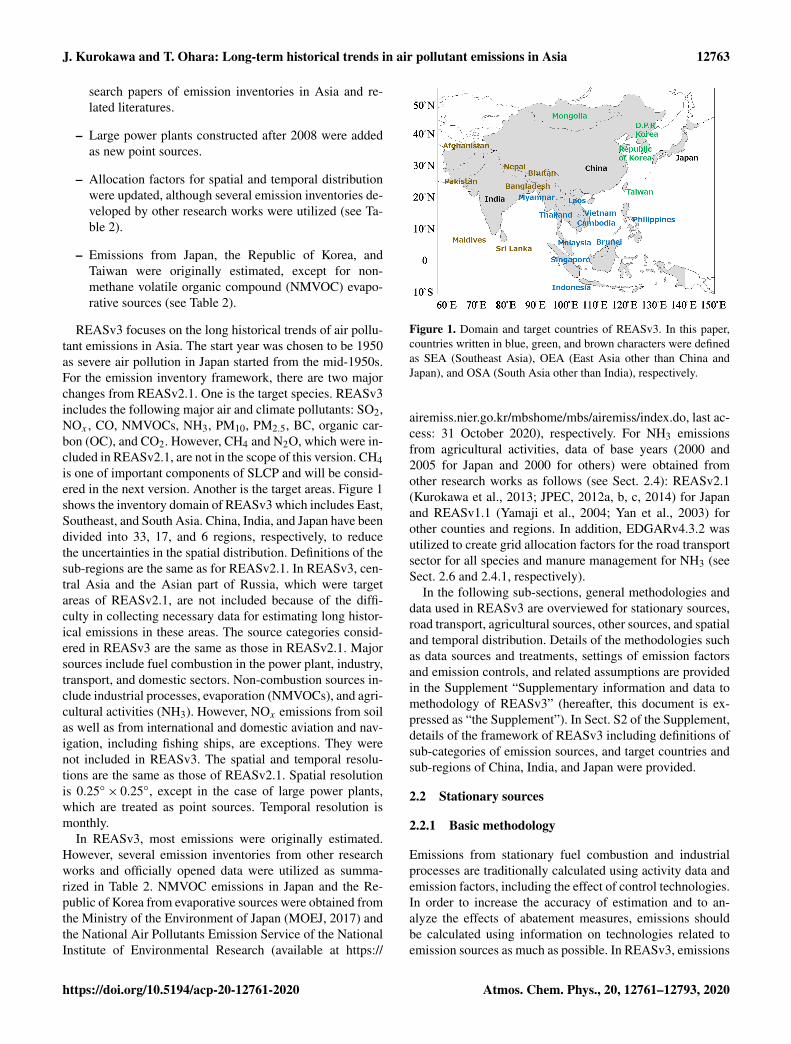
REASv3 focuses on the long historical trends of air pollu-tant emissions in Asia. The start year was chosen to be 1950as severe air pollution in Japan started from the mid-1950s.For the emission inventory framework, there are two majorchanges from REASv2.1. One is the target species. REASv3includes the following major air and climate pollutants: SO2,NOx , CO, NMVOCs, NH3, PM10, PM2.5, BC, organic car-bon (OC), and CO2. However, CH4 and N2O, which were in-cluded in REASv2.1, are not in the scope of this version. CH4is one of important components of SLCP and will be consid-ered in the next version. Another is the target areas. Figure 1shows the inventory domain of REASv3 which includes East,Southeast, and South Asia. China, India, and Japan have beendivided into 33, 17, and 6 regions, respectively, to reducethe uncertainties in the spatial distribution. Definitions of thesub-regions are the same as for REASv2.1. In REASv3, cen-tral Asia and the Asian part of Russia, which were targetareas of REASv2.1, are not included because of the diffi-culty in collecting necessary data for estimating long histor-ical emissions in these areas. The source categories consid-ered in REASv3 are the same as those in REASv2.1. Majorsources include fuel combustion in the power plant, industry,transport, and domestic sectors. Non-combustion sources in-clude industrial processes, evaporation (NMVOCs), and agri-cultural activities (NH3). However, NOx emissions from soilas well as from international and domestic aviation and nav-igation, including fishing ships, are exceptions. They werenot included in REASv3. The spatial and temporal resolu-tions are the same as those of REASv2.1. Spatial resolutionis 0.25◦× 0.25◦, except in the case of large power plants,which are treated as point sources. Temporal resolution ismonthly.
In REASv3, most emissions were originally estimated.However, several emission inventories from other researchworks and officially opened data were utilized as summa-rized in Table 2. NMVOC emissions in Japan and the Re-public of Korea from evaporative sources were obtained fromthe Ministry of the Environment of Japan (MOEJ, 2017) andthe National Air Pollutants Emission Service of the NationalInstitute of Environmental Research (available at https://
Figure 1. Domain and target countries of REASv3. In this paper,countries written in blue, green, and brown characters were definedas SEA (Southeast Asia), OEA (East Asia other than China andJapan), and OSA (South Asia other than India), respectively.
airemiss.nier.go.kr/mbshome/mbs/airemiss/index.do, last ac-cess: 31 October 2020), respectively. For NH3 emissionsfrom agricultural activities, data of base years (2000 and2005 for Japan and 2000 for others) were obtained fromother research works as follows (see Sect. 2.4): REASv2.1(Kurokawa et al., 2013; JPEC, 2012a, b, c, 2014) for Japanand REASv1.1 (Yamaji et al., 2004; Yan et al., 2003) forother counties and regions. In addition, EDGARv4.3.2 wasutilized to create grid allocation factors for the road transportsector for all species and manure management for NH3 (seeSect. 2.6 and 2.4.1, respectively).
In the following sub-sections, general methodologies anddata used in REASv3 are overviewed for stationary sources,road transport, agricultural sources, other sources, and spatialand temporal distribution. Details of the methodologies suchas data sources and treatments, settings of emission factorsand emission controls, and related assumptions are providedin the Supplement “Supplementary information and data tomethodology of REASv3” (hereafter, this document is ex-pressed as “the Supplement”). In Sect. S2 of the Supplement,details of the framework of REASv3 including definitions ofsub-categories of emission sources, and target countries andsub-regions of China, India, and Japan were provided.
2.2 Stationary sources
2.2.1 Basic methodology
Emissions from stationary fuel combustion and industrialprocesses are traditionally calculated using activity data andemission factors, including the effect of control technologies.In order to increase the accuracy of estimation and to an-alyze the effects of abatement measures, emissions shouldbe calculated using information on technologies related toemission sources as much as possible. In REASv3, emissions
https://doi.org/10.5194/acp-20-12761-2020 Atmos. Chem. Phys., 20, 12761–12793, 2020

12764 J. Kurokawa and T. Ohara: Long-term historical trends in air pollutant emissions in Asia
Table 1. General information on REASv3.
Item Description
Species SO2, NOx , CO, NMVOCs, NH3, CO2, PM10, PM2.5, BC, and OC
Years 1950–2015
Areas East, Southeast, and South Asia
Emission sources Fuel combustion in the power plant, industry, transport, and domestic sectors;industrial processes; agricultural activities (fertilizer application and livestock);and others (fugitive emissions, solvent use, human, etc.)
Spatial resolution 0.25◦ by 0.25◦
Temporal resolution Monthly
Data distribution https://www.nies.go.jp/REAS/index.html (last access: 31 October 2020)
Table 2. Emission inventories from other research works and officially opened data utilized in REASv3.
Other emission inventories and data sources How utilized in REASv3
VOC Emission Inventory in Japan (MOEJ, 2017) Evaporative emissions of NMVOCs in Japana
The National Air Pollutants Emission Service of theNational Institute of Environmental Research (https://airemiss.nier.go.kr/mbshome/mbs/airemiss/index.do,last access: 31 October 2020)
Evaporative emissions of NMVOCs in the Republic ofKoreaa
REASv2.1 (Kurokawa et al., 2013; JPEC, 2012a, b, c,2014)
NH3 emissions from agricultural sources in Japanb
REASv1.1 (Yamaji et al., 2004; Yan et al., 2003) NH3 emissions from agricultural sources in countriesand regions other than Japanb
REASv2.1 (Kurokawa et al., 2013; JPEC, 2012a, b, c,2014)
Grid allocation factors for the manure managementc
and road transportd sectors for Japan
EDGARv4.3.1 (Crippa et al., 2016) Grid allocation factors for the manure managementc
and road transportd sectors for countries and regionsother than Japan
a See Sect. S5.3 of the Supplement. b See Sect. 2.4. c See Sect. S9.1 of the Supplement. d See Sect. 2.6.
from stationary combustion and industrial processes are esti-mated based on the following equation:
E =∑
i
∑j
∑k,l{Ai,j ×Fi,j,k,l ×EFi,j,k × (1−Ri,j,l)}, (1)
where E represents emission, i is the type of activity data,j is the type of sector category, k is the type of technologyrelated to emission factor, l stands for the control technol-ogy after emission, A is the amount of activity data, EF isthe emission factor of each technology, R is the removal ef-ficiency of each technology, and F is the fraction rate of ac-tivity data for a combination of i, j , k, and l. When SO2emissions from combustion sources are estimated using sul-fur contents of fuels, EFi,j,k in Eq. (1) is calculated as fol-lows:
EFi,j,k = NCVi,j × Si,j × (1−SRi,j,k)× 2, (2)
where NCV is the net calorific value of fuel, S is the sulfurcontent of fuel, and SR is the sulfur retention in ash for acombination of i, j , and k; 2 is a factor to convert the valueof S to SO2.
Unfortunately, in the case of Asia, information availableon emission factors and removal efficiencies is limited. Eventhough there is information on the introduction rates of tech-nologies for both emission factors and removal efficiencies,they are available independently. Therefore, for most cases,an average of the removal efficiencies is calculated using thevalues of each abatement equipment and its penetration rate.Then, the average removal efficiencies are commonly used tocalculate the emission factors of each technology.
Note that several sub-sectors in stationary sources suchas coke production and the cement industry include both
Atmos. Chem. Phys., 20, 12761–12793, 2020 https://doi.org/10.5194/acp-20-12761-2020
J. Kurokawa and T. Ohara: Long-term historical trends in air pollutant emissions in Asia 12765
combustion and non-combustion emission sources. SeeSects. S2.4.1 and S2.4.2 of the Supplement for details.
2.2.2 Activity data
Fuel consumption is the core activity data of the emissioninventory of air pollutants and greenhouse gases. For mostcountries, the amount of energy consumption for each fueltype and sector was primarily obtained from the InternationalEnergy Agency (IEA) World Energy Balances (IEA, 2017).For China, province-level tables in the China Energy Sta-tistical Yearbook (CESY) (National Bureau of Statistics ofChina, 1986, 2001–2017) were used. For countries and re-gions whose energy data are not included in IEA (2017),fuel consumption data were taken from the United Nations(UN) Energy Statistics Database (UN, 2016) and the UNdata, which is a web-based data service of the UN (https://data.un.org/, last access: 31 October 2020). See Sect. S3.1.1of the Supplement for definitions of fuel types.
One major obstacle in this study was collecting activitydata for the entire target period of REASv3, that is, from1950 to 2015. IEA (2017) includes data from Japan dur-ing 1960–2015 and those from other countries during 1971–2015; however, for many countries, fuel types, and sectorcategories, the oldest years when data exist are more laterthan 1971. Furthermore, past data for sectors do not con-tain as many categories. For example, coal consumption datain detailed sub-categories of the industrial sector existed inIndonesia only after 2000, but corresponding data are onlyavailable for the industry total before 1999. In this case, rel-ative ratios of fuel consumption in detailed sub-categories tototal industry in 2000 were used to distribute the total in-dustry data to each sub-category for the years before 1999.This procedure is performed for similar cases for all sectorsand sometimes for total final consumption. In cases wheredata did not exist beyond a certain year, fuel consumptiondata were extrapolated using trends of related data for eachsub-category. For example, power generation and amount ofindustrial products were used to observe trends of fuel con-sumption in power plants and each industry’s sub-category,respectively. Data for long historical trends were obtainedfrom a variety of sources. For example, power generationdata and amounts of major industrial products were ob-tained from Mitchell (1998), and national and internationalstatistics as well as related literatures were surveyed. SeeSect. S3.1.2 of the Supplement for details of data sources offuel consumption and assumptions to estimate missing his-torical data. For China, data of CESY for each province wereavailable from 1985 to 2015. During 1950–1984, first, totalenergy data in China were developed based on IEA (2017),and then fuel consumption in each province was extrapo-lated using the total data of China in each fuel type and sec-tor category. See Sect. S3.1.3 of the Supplement for detailsof regional fuel consumption data in China. For countrieswhich used the Energy Statistics Database, fuel consumption
of each fuel and sector was taken from the UN data (avail-able at https://data.un.org/, last access: 31 October 2020) forthe period between 1990 and 2015 and was extrapolated us-ing the trend of total consumption of each fuel type obtainedfrom the UN Energy Statistics Database.
As described in Sect. 2.1, India and Japan have 17 and6 sub-regions, respectively. Therefore, for them, country to-tal data of IEA (2017) need to be divided for each sub-region. For Japan, energy consumption statistics of each pre-fecture that were obtained from the Agency for Natural Re-sources and Energy (available at https://www.enecho.meti.go.jp/statistics/energy_consumption/ec002/results.html, lastaccess: 31 October 2020) were used as default weight-ing factors to allocate country total data to the six re-gions. Similarly, for India, default weighting factors forregional allocation were estimated from the TERI (TheEnergy and Resources Institute) Energy & EnvironmentData Diary and Yearbook (TERI, 2013, 2018), Annual Sur-vey of Industries (Ministry of Statistics & Programme Im-plementation, available at http://www.csoisw.gov.in/cms/en/1023-annual-survey-of-industries.aspx, last access: 31 Oc-tober 2020), and Census of India (Chandramouli, 2011),among others. In general, details of these weighting factorsare less than those of the country’s total fuel consumption.In addition, these data are not available for all the yearsduring 1950–2015. Therefore, regional allocation factors forsome sectors were developed independently if correspond-ing proxy data were available. For the power plant sector,generation capacities of each region and year were calcu-lated as proxy data using the World Electric Power PlantsDatabase (WEPP) (Platts, 2018). For India, traffic volumes(see Sect. 2.3.1) and amount of industrial production in eachregion (see the last paragraph of this section) were used asproxy data. Details of regional fuel consumption data in In-dia and Japan were provided in Sect. S3.1.4. and S3.1.5, re-spectively.
Similarly to REASv2.1, large power plants are treatedas point sources in REASv3 and are updated based onthe REASv2.1 database. Before 2007, power plants thatwere classified as point sources were the same as those inREASv2.1, and their information, such as generating capaci-ties and start and retire years, was updated using WEPP. Dur-ing 2000 to 2007, fuel consumption data were the same asthose in REASv2.1. In REASv3, power plants whose startyears were after 2007 and generation capacities were largerthan 300 MW were added as new point sources. Fuel con-sumption of new power plants were estimated based on rela-tions between fuel consumption amounts and generation ca-pacities of the point data in REASv2.1. If the (A) total fuelconsumption of each power plant in a country was larger than(B) the corresponding data in the power plant sector, valuesof each power plant were adjusted by ratios of (B) per (A).If (B) was larger than (A), differences between (B) and (A)were treated as data of area sources. See also Sect. S3.1.6 ofthe Supplement for fuel consumption data in power plants.
https://doi.org/10.5194/acp-20-12761-2020 Atmos. Chem. Phys., 20, 12761–12793, 2020

12766 J. Kurokawa and T. Ohara: Long-term historical trends in air pollutant emissions in Asia
For emissions from industrial processes, activity data in-cluded the amount of industrial products. Correspondingdata were mainly obtained from related international statis-tics and national statistics. For example, iron and steel pro-duction data were taken from the Steel Statistical Year-book (World Steel Association, 1978–2016) and data fornon-ferrous metals and non-metallic minerals were obtainedfrom the United States Geological Survey (USGS) Miner-als Yearbook (USGS, 1994–2015). Brick production datawere obtained from a variety of sources, such as Zhang(1997), Maithel (2013), Klimont et al. (2017), and the UNdata. For China and India, the authors also used Internetdatabase services, namely China Data Online (https://www.china-data-online.com/, last access: 31 October 2020) andIndiastat (https://www.indiastat.com/, last access: 31 Octo-ber 2020), respectively, which provided both national andregional statistics. The USGS Minerals Yearbook (USGS,1994–2015) also provided information on plants in each sub-region of China, India, and Japan. Data in the aforementionedstatistics were not available for the early years of the targetperiod of REASv3. In such cases, data of Mitchell (1998)were used as factors to extrapolate the activity data until1950. Details of activity data related to industrial productionand other transformation were given in Sect. S4.1 of the Sup-plement.
2.2.3 Emission factors
Setting up emission factors and removal efficiencies for sta-tionary combustion and industrial processes is a difficult pro-cedure, especially for a long historical emission inventory.In this study, emission factors without effects of abatementmeasures were set, which were used for the entire targetperiod of REASv3. Then, effects of control measures wereset considering their temporal variations, both for abatementmeasures before emissions such as using low-sulfur fuels andlow-NOx burners and those after emissions such as flue gasdesulfurization (FGD) and electrostatic precipitator (ESP).These settings were done for each country and region basedon country- and region-specific information. However, suchinformation is still limited, especially in the Asian region.Therefore, default values of unabated emission factors wereselected, and default removal efficiencies were set to zero.Then, these default values were updated in case informationand the literature on each country and region were available.For default emission factors, the majority of settings werecontinuously used from REASv2.1, but some of them, in-cluding effects to control measures (net emission factors),were changed to unabated emission factors. Default emissionfactors were mainly obtained from Kato and Akimoto (1992)for SO2 and NOx ; Bond et al. (2004), Kupiainen and Klimont(2004), and Klimont et al. (2002, 2017) for PM species; the2006 IPCC Guidelines for National Greenhouse Gas Inven-tories (IPCC, 2006) for CO2; and the AP-42 (US EPA, 1995),the Global Atmospheric Pollution Forum Air Pollutant Emis-
sion Inventory Manual (Vallack and Rypdal, 2012), Shresthaet al. (2013), the EMEP/EEA emission inventory guidebook2016 (EEA, 2016), and other literatures for others (see thelast paragraph of this sub-section).
For country- and region-specific settings, in addition to lit-eratures used in REASv2.1 (see Kurokawa et al., 2013), newinformation, especially for technologies related to settings ofemission factors and removal efficiencies, was surveyed. Al-though such information is still limited in Asia, the volumeof accessible information on China is relatively large. Gen-eral information on China in recent years was mainly ob-tained from Li et al. (2017b) and Zheng et al. (2018). In-troduction rates of technologies were obtained from Hua etal. (2016) for cement, Wu et al. (2017) for iron and steel,Huo et al. (2012a) for coke ovens, and Zhao et al. (2013,2014, and 2015) for a variety of sources. For India, infor-mation for technology settings was mainly taken from Sa-davarte and Venkataraman (2014), Pandey et al. (2014), Gut-tikunda and Jawahar (2014), and Reddy and Venkataraman(2002a). For power plants, the WEPP database has elementsfor installed equipment to control SO2, NOx , and PM specieswhich were used for settings of emission factors and removalefficiencies of power plants treated as point sources. How-ever, these data are not available for most power plants, es-pecially in Asia. Therefore, in the case of South and South-east Asia, a variety of literatures, such as Sloss (2012) andUN Environment (2018), were referred to, to set emissionfactors and removal efficiencies. For Japan, introduction ofcontrol technologies for air pollutants was initiated earlierthan other countries in Asia. A lot of domestic reports forair pollution and control technologies in power and industryplants published in Japanese, such as MRI (2015), Shimoda(2016), Suzuki (1990), and Goto (1981), were referred to,to determine emission factors, removal efficiencies, and theirtemporal variations.
Details of emission factors and settings of emission con-trols for stationary combustion sources were provided inSect. S3.2 of the Supplement. Those for stationary non-combustion emissions from the industrial production andother transformation sectors were described in Sect. S4.2.Activity data and emission factors of NMVOCs from thechemical industry were obtained from Sect. S5.1.5 andS5.2.5, respectively. Those for NH3 emissions from indus-trial production were provided in Sect. S8.3.
2.3 Road transport
2.3.1 Basic methodology
The methodology for the road transport sector is the same asthat of REASv2.1. Equations to estimate hot and cold startemissions (except for SO2 and CO2) are as follows:
EHOT =∑
i{NVi ×ADTi ×EFHOTi}, (3)
Atmos. Chem. Phys., 20, 12761–12793, 2020 https://doi.org/10.5194/acp-20-12761-2020

J. Kurokawa and T. Ohara: Long-term historical trends in air pollutant emissions in Asia 12767
where EHOT is the hot emission, i is the vehicle type, NVis the number of vehicles in operation, ADT is the annualdistance traveled, and EFHOT is the emission factor. SO2emissions are calculated using sulfur contents in gasolineand diesel consumed in the road transport sector, assumingsulfur retention in ash is zero. CO2 emissions are estimatedby calculating the consumption amounts of fuels (gasoline,diesel, liquefied petroleum gas, and natural gas) and the cor-responding emission factors (IPCC, 2006). Details for SO2and CO2 from road transport were described in Sect. S6.2.3of the Supplement.
Cold start emissions (ECOLD) are estimated for NOx , CO,PM10, PM2.5, BC, OC, and NMVOCs using the followingequation:
ECOLD =∑
i{NVi ×ADTi ×EFHOTi ×βi(T )×Fi(T )}, (4)
where β is the fraction of distance traveled driven with a coldengine or with the catalyst operating below the light-off tem-perature, and F is the correction factor of EFHOT for coldstart emissions. β and F are functions of temperature T andare taken from EEA (2016) (see Sect. S6.2.1 of the Supple-ment for additional information on the settings). For Japan,the ratios of cold start and hot emissions for each vehicletype were estimated from the JEI-DB. Then, cold start emis-sions were calculated by hot emissions and the ratios for eachvehicle type. In REASv3, effects of regulations on cold startemissions were ignored and need to be considered in the nextversion.
For evaporation from gasoline vehicles, emissions (EEVP)were estimated using the following equation of Tier 1 of EEA(2016):
EEVP =∑
i{NVi ×EFEVPi(T )}, (5)
where EFEVP is the emission factor as a function of tem-perature. For Japan, evaporative emissions in 2000, 2005,and 2010 were obtained from the JEI-DB and those between2000 (2005) and 2005 (2010) were interpolated. For emis-sions before 2000 and after 2010, emissions from runningloss were extrapolated using trends of traffic volume, andthose from hot soak loss and diurnal breaking loss were ex-trapolated by trends of vehicle numbers. See Sect. S6.3 of theSupplement for the NMVOC evaporative emissions.
2.3.2 Activity data
Basic activity data of the road transport sector include thenumber of vehicles in operation for each type. Data on theregistered number of vehicles are available in the nationalstatistics of each country and the World Road Statistics (IRF,1990–2018). If these statistics did not contain data until1950, the numbers were extrapolated using trends of data foraggregated vehicle categories in Mitchell (1998). For China,data for each sub-region were obtained from the China Statis-tical Yearbook (National Bureau of Statistics of China, 1986–2016) and China Data Online. Those for India were taken
from the TERI Energy & Environment Data Diary and Year-book (TERI, 2013, 2018) and Indiastat. A problem that wasencountered was that registered vehicles were not always inoperation. For India, the number of vehicles obtained as reg-istered vehicles was corrected based on Baidya and Borken-Kleefeld (2009) and Prakash and Habib (2018). For othercountries, the number of registered vehicles was consideredto be those in operation due to a lack of information. In ad-dition, to estimate emissions, these numbers must be furtherdivided into vehicles based on each fuel type. However, suchinformation is not easily available in national statistics. Inthis study, settings of Streets et al. (2003a) and REASv2.1were used as the default and were updated if national in-formation was available, such as He et al. (2005), Yan andCrookes (2009), Sahu et al. (2014), and Malla (2014). If thenumber of LPG and CNG vehicles were available only forrecent years, data were extrapolated using amounts of fuelconsumption in the road transport sector in IEA (2017).
Emission factors of the road transport sector used in thisstudy were given as emission amounts per traffic volumes.Therefore, annual vehicle kilometers traveled (VKT) pereach vehicle type need to be set for each country. We useddata of Clean Air Asia (2012) for many countries. Clean AirAsia (2012) includes data for China and India, but data ofChina were estimated based on Huo et al. (2012b), and thoseof India were set following Prakash and Habib (2018) andPandey and Venkataraman (2014). For Japan, the total an-nual VKT for detailed vehicle types were obtained from re-ports of the Pollutants Release and Transfer Register pub-lished by the Ministry of Economy, Trade and Industry until2001 (METI, 2003–2017), which was originally estimatedfrom the Road Transport Census of Japan developed by theMinistry of Land, Infrastructure, Transport and Tourism. Be-fore 2001, the total annual VKT was extrapolated using dataof more aggregated vehicle categories in the Annual Reportof Road Statistics (MLIT, 1961–2016) until 1960 and fromthe Historical Statistics of Japan (Japan Statistical Associa-tion, 2006) until 1950.
Details of the number of vehicles and annual vehicle kilo-meters traveled were described in Sect. S6.1.1 of the Supple-ment.
2.3.3 Emission factors
For most countries, road transport is one of the major causesof air pollution. In many Asian countries, vehicle emissionstandards were introduced after the late 1990s and werestrengthened in phases (Clean Air Asia, 2014). Therefore, forroad vehicles, year-to-year variation of emission factors mustbe taken into account for a long historical emission inventory.In REASv3, emission factors of NOx , CO, NMVOCs, andPM species for exhaust emissions from road vehicles wereestimated by following procedures.
1. Emission factors of each vehicle type in a base yearwere estimated.
https://doi.org/10.5194/acp-20-12761-2020 Atmos. Chem. Phys., 20, 12761–12793, 2020

12768 J. Kurokawa and T. Ohara: Long-term historical trends in air pollutant emissions in Asia
2. Trends of the emission factors for each vehicle typewere estimated considering the timing of road vehicleregulations in each country and the ratios of vehicle pro-duction years.
3. Emission factors of each vehicle type during the targetperiod of REASv3 were calculated using those of baseyears and the corresponding trends.
The information on road vehicle regulations in each coun-try and region was taken from Clean Air Asia (2014). For theratios of vehicle production years, due to lack of informa-tion, data for Macau derived from Zhang et al. (2016) wereused for Hong Kong, the Republic of Korea, and Taiwan,and those from the Japan Environmental Sanitation Centerand Suuri Keikaku (2011) for Vietnam were used for othercountries and regions. Then, trends of emission factors wereestimated using the above data and information with val-ues of Europe and United States standards. Finally, emis-sion factors used to estimate emissions were calculated foreach vehicle type. For most countries, the years just be-fore the regulations for road vehicles began were set as baseyears, and non-controlled emission factors that were used inREASv1.1 and REASv2.1 were adopted for emission factorsof the base years. Countries for which information on reg-ulations was not obtained, the non-controlled emission fac-tors, were used for the entire target period of REASv3. ForChina and India, emission factors in 2010 were estimated asthe base year’s data using recently published papers, suchas Huo et al. (2012b), Xia et al. (2016), Mishra and Goyal(2014), and Sahu et al. (2014). For the Republic of Koreaand Taiwan, whose emissions were not originally estimatedin REASv2.1, emission factors were estimated with highuncertainties based on values of Europe and United Statesstandards, respectively. For Japan, emission factors for eachemission standard are available for several vehicle speeds(JPEC, 2012a). Combining these data with information forannual VKT of each vehicle speed, ratios of vehicle ages, andtime series of regulation standards, emissions of road trans-port in Japan were calculated. Details of emission factors ofexhaust emissions were provided in Sect. S6.2 of the Supple-ment.
2.4 Agricultural sources
REASv3 includes NH3 emissions from manure managementand fertilizer application in agricultural sources. Approachessimilar to REASv2.1 were adopted to estimate historicalemissions and develop monthly gridded data. First, annualemissions of each country and sub-region except for Japanand their gridded data for the year 2000 were selected fromREASv1.1 (Yamaji et al., 2004; Yan et al., 2003) as basedata. For Japan, corresponding base data were obtained fromREASv2.1 (Kurokawa et al., 2013: JPEC, 2012a, b, c, 2014)for the years 2000 and 2005. Second, trends of emissionsduring 1950–2015 were estimated for each country and sub-
region. Third, annual emissions for the period were calcu-lated using the trends and base data. Fourth, changes in spa-tial distribution from base years to target years and monthlyvariations in each country and sub-region were estimated.Finally, monthly gridded data of emissions were developedfor 1950–2015. For Japan, emission data during 2001–2004were interpolated between those in 2000 and 2005. Detailsfor manure management and fertilizer application are givenin Sect. 2.4.1 and 2.4.2, respectively.
2.4.1 Manure management
Trends in NH3 emissions from manure management of live-stock, except for its application as fertilizer, were estimatedbased on the Tier 1 method of EEA (2016). In this method,emissions are calculated based on the numbers of live-stock and the corresponding emission factors. Statistics onthe number of animals, such as broilers, dairy cow, andswine, are mainly obtained from FAOSTAT (available athttp://www.fao.org/faostat/en/, last access: 31 October 2020)of the Food and Agriculture Organization (FAO) of the UNfrom the period between 1961 and 2015. For the years be-fore 1960, data were obtained from Mitchell (1998). Nationalstatistics were surveyed for data on provinces, states, andprefectures in China, India, and Japan, respectively, to de-velop activity data for each sub-region. Emission factors areobtained from EEA (2016). For spatial distribution, changesin grid allocation for each country and sub-region from theyear 2000 were estimated using EDGARv4.3.2 from 1970 to2012. Grid allocation factors in 1970 and 2012 were used forthe period before and after 1970 and 2012, respectively. Fortemporal variations, monthly allocation factors are estimatedas a function of temperature by referring to the monthlyvariations of emissions in Japan based on the JEI-DB. De-tailed methodologies and data sources for manure manage-ment were provided in Sect. S8.1 in the Supplement.
2.4.2 Fertilizer
In most countries, fertilizer application is the largest sourceof NH3 emissions. Emission trends after the application ofmanure and synthetic N fertilizer were estimated using EEA(2016). Manure application is one of the processes of manuremanagement, whose emission trend was calculated based onthe number of animals and the corresponding emission fac-tor. For synthetic N fertilizer, trends of total consumptionof fertilizer were used in REASv2.1. However, this simpleapproach causes uncertainties because emission factors aredifferent among types of fertilizer (EEA, 2016). Therefore,in REASv3, emissions from each N fertilizer, such as am-monium phosphate and urea, were estimated separately, andtrends in total emissions were calculated. For spatial distri-bution, changes in grid allocation factors for each countryand sub-region from the year 2000 were estimated using ahistorical global N fertilizer application map during 1961–
Atmos. Chem. Phys., 20, 12761–12793, 2020 https://doi.org/10.5194/acp-20-12761-2020

J. Kurokawa and T. Ohara: Long-term historical trends in air pollutant emissions in Asia 12769
2010, developed by Nishina et al. (2017). Data for 1961 and2010 were used for the period before 1961 and after 2010, re-spectively. For seasonal variations, monthly factors of Chinaand Japan were determined based on Kang et al. (2016)and the JEI-DB, respectively. For other countries, data fromNishina et al. (2017) have monthly application amounts ineach grid. However, there are cases that some months havehigh factors, whereas the others have almost zero. Referringto Janssens-Maenhout et al. (2015), we adopted the conser-vative way such that the highest monthly factor was set at 0.2and the factors of all months were adjusted accordingly. SeeSect. S8.2 for details of methodologies and data sources foremissions from fertilizer application.
2.5 Other sources
NMVOC emissions from evaporative sources are increas-ing significantly in Asia along with economic growth. Ma-jor sources of NMVOC emissions include usage of solventsfor dry cleaning, degreasing operations, and adhesive appli-cation as well as for paint use. Fugitive emissions related tofossil fuels, such as extraction and handling of oil and gas, oilrefinery, and gasoline stations, are also important. However,statistics on activity data and information of emission fac-tors for these sources are often less available than those forfuel combustion and industrial processes. In this study, de-fault activity data and emission factors were obtained fromREASv2.1 and were updated if information was available inrecently published papers (such as Wei et al. 2011, for China,and Sharma et al., 2015, for India). In general, activity dataof the past years are not available, and, in such cases, proxydata are prepared for trend factors. For example, populationnumbers were used for dry cleaning and production numbersof vehicles were used for paint application for automobilemanufacturing. GDP was used for default trend factors. Foremission calculation, the same equation for stationary com-bustion was adopted. Details of activity data and emissionfactors for non-combustion sources of NMVOCs were pro-vided in Sect. S5 of the Supplement.
In addition to agricultural activities, latrines are an impor-tant source of NH3, especially in rural areas. Activity dataare population numbers in no sewage service areas estimatedreferring settings of REASv2.1 and emission factors werebased on EEA (2016) and Vallack and Rypdal (2012). Also,humans themselves are sources of NH3 emissions throughperspiration and respiration. For these sources, populationnumbers are activity data mainly taken from UN (2018) andemission factors are obtained from EEA (2016). The equa-tion to estimate emission is also the same as that of stationarycombustion. Additional data and information for emissionsfrom human and latrines were described in Sect. S8.4 andS8.5, respectively.
In REASv3, aviation and ship emissions, including fishingships, are not included, but emissions of fuel combustion inother transport sectors (namely, except for aviation, naviga-
tion, and road), such as railway and pipeline transport, wereestimated. Equation (1) is also used for estimating emissionsof these sources. See Sect. S7 of the Supplement for addi-tional data and information for other transport sectors.
2.6 Spatial and temporal distribution
Procedures for developing gridded emission data were thesame as those of REASv2.1. Large power plants were treatedas point sources, and longitude and latitude of each powerplant were provided. Positions of power plants were surveyedbased on detailed information, such as names of units, plants,and companies from WEPP (Platts, 2018). These weresearched on Internet sites, such as Industry About (https://www.industryabout.com/, last access: 31 October 2020) andGlobal Energy Observatory (http://globalenergyobservatory.org/, last access: 31 October 2020). Positions for newlyadded power plants in REASv3 as well as those in REASv2.1were surveyed because some of these services were not avail-able when REASv2.1 was developed. For cement, iron, andsteel plants (and non-ferrous metal plants in Japan), REASv3still did not treat them as point sources due to a lack of ac-tivity data. However, positions, production capacities, andstart and retire years for large plants were surveyed similarlyto power plants and used for developing allocation factorsfor corresponding sub-sectors. For the road transport sec-tor, REASv2.1 used coarse grid allocation data of REASv1.1with 0.5◦× 0.5◦ resolution. Therefore, in REASv3, grid al-location factors for each country and sub-region, exceptJapan, were updated using gridded emission data of the roadtransport sector of EDGARv4.3.2 during 1970–2012. Before1970 (after 2012), data for 1970 (2012) were used. For Japan,gridded emission data of the JEI-DB in 2000, 2005, and 2010were used to develop grid allocation factors. For the years be-tween 2000 (2005) and 2005 (2010), the JEI-DB data wereinterpolated. For years before 2000 (after 2010), the JEI-DBdata for 2000 (2010) were used. For the residential sectors,rural, urban, and total populations of HYDE 3.2.1 (KleinGoldewijk et al., 2017) with 5′× 5′ were used to create allo-cation factors. Data of HYDE 3.2.1 were available for 1950,1960, 1970, 1980, 1990, 2000, 2005, 2010, and 2015, andthe years between them were interpolated. Spatial distribu-tions of the total population were used for grid allocation ofall other sources. Detailed methodologies and data sourcesfor grid allocation were provided in Sect. S9.1 in the Supple-ment.
The methodology to estimate monthly emission data inREASv3 was the same as that of REASv2.1. In gen-eral, monthly emissions were estimated by allocating an-nual emissions to each month using monthly proxy data.Monthly generated power and production amounts of in-dustrial products were used as the monthly allocation fac-tors for the power plant sector and the corresponding in-dustry sub-sectors, respectively. Basically, monthly factorsof REASv2.1 during 2000–2008 were also used in REASv3
https://doi.org/10.5194/acp-20-12761-2020 Atmos. Chem. Phys., 20, 12761–12793, 2020

12770 J. Kurokawa and T. Ohara: Long-term historical trends in air pollutant emissions in Asia
and were extended if data existed before (after) 2000 (2008).For the years where surrogate data were unavailable, thedata of the oldest (newest) year were used before (after)the year. For brick production, monthly allocation factorsfor Southeast and South Asian countries were estimatedby referring to Maithel et al. (2012) and Maithel (2013).For the residential sector, monthly variations of emissionswere estimated using surface temperature in each grid cell,similarly to REASv2.1. Surface temperatures during 1950–2015 were taken from NCEP reanalysis data provided by theNOAA/OAR/ESRL PSD, Boulder, Colorado, USA (https://psl.noaa.gov/data/gridded/data.ncep.reanalysis.html, last ac-cess: 31 October 2020). For Thailand and Japan, mostmonthly factors were set based on country-specific informa-tion from Pham et al. (2008) and JPEC (2014), respectively.See Sect. S9.2 of the Supplement for details of monthly vari-ation factors.
3 Results and discussion
3.1 Trends of Asian and national emissions
Trends in air pollutant emissions from Asia, China, India,Japan, and other countries are described in this section,mainly focusing on SO2, NOx , and BC emissions as theyhave important roles in both air pollution and climate change.SO2 and NOx are precursors of sulfate and nitrate aerosols,respectively, which are the major components of secondaryPM2.5. NOx is also a precursor of ozone. Furthermore, BCis a major component of primary PM2.5. PM2.5 and ozonenot only harm human health and ecosystems, but also influ-ence climate change. BC and ozone have a warming effecton climate change, whereas sulfate and nitrate aerosols havea cooling effect. Note that all the air pollutant emissions frommajor countries and regions between 1950 and 2015 catego-rized based on major sectors and fuel types are provided inthe Supplement (Figs. S1–S12). CO2 emissions in REASv3include contribution from biofuel combustion unless other-wise indicated.
3.1.1 Asia
Table 3 summarizes the national emissions of each species in2015 and the total emissions from Asia in 1950, 1960, 1970,1980, 1990, 2000, and from 2010 to 2015. Figure 2 showsemissions of SO2, NOx , CO, NMVOCs, NH3, CO2, PM10,PM2.5, BC, and OC in China, India, Japan, Southeast Asia(SEA), East Asia other than China and Japan (OEA), andSouth Asia other than India (OSA) from 1950 to 2015. Av-erage total emissions in Asia during 1950–1955 and 2010–2015 (growth rates in these 60 years estimated from thetwo averages) are as follows: SO2: 3.2 Tg, 42.4 Tg (13.1);NOx : 1.6 Tg, 47.3 Tg (29.1); CO: 56.1 Tg, 303 Tg (5.4);NMVOCs: 7.0 Tg, 57.8 Tg (8.3); NH3: 8.0 Tg, 31.3 Tg (3.9);CO2: 1.1 Pg, 18.6 Pg (16.5) (CO2 excluding biofuel com-
bustion 0.3 Pg, 16.8 Pg (48.6)); PM10: 5.9 Tg, 30.2 Tg (5.1);PM2.5: 4.6 Tg, 21.3 Tg (4.6); BC: 0.69 Tg, 3.2 Tg (4.7); andOC: 2.5 Tg, 6.6 Tg (2.7). Clearly, all the air pollutant emis-sions in Asia increased significantly during these 6 decades.However, this increase was different among the aforemen-tioned species. Growth rates of emissions were relativelylarge for SO2, NOx , and CO2 because the major sources ofthese species are power plants, industries, and road transport,for which fuel consumption increased significantly alongwith economic development in Asia. SO2 increased beforethe other species because the majority of the emissions wereobtained from the combustion of coal, which is easier toobtain than oil and gas. SO2, NOx , and CO2 emissions in-creased keenly in the early 2000s along with rapid growthof emissions of these species in China. For NOx , combus-tion of oil fuels, especially by road vehicles, contributed toa large growth of emissions in the latter half of 1950–2015.Growth rates of NMVOCs have also increased recently dueto an increase in the emissions from road vehicles and evapo-rative sources, such as paint and solvent usage, in accordancewith economic growth of Asian countries. On the other hand,rates of growth of CO, PM10, PM2.5, BC, and OC are rela-tively small. One reason is that emissions of these species aremainly from incomplete combustion in low temperature, andthus emissions from power plants and large industry plantsare relatively small. Another reason is that a major sourceof these species is the combustion of coal and biofuels inthe residential sector, which dominated over other sectors inearlier times and was relatively large even in recent years inAsia. Recently, emissions of these species from industries,including combustion and non-combustion processes, havebeen increasing. In addition, gasoline and diesel vehicleshave contributed recently to the growth of CO and BC emis-sions, respectively. Agricultural activities, such as manuremanagement of livestock and fertilizer application, which aremajor sources of NH3, are rising to support a growing popu-lation in Asia. Although the growth rate of NH3 emissions issmaller than other species, it still shows an increasing trend.
Differences in the trends of emissions were also observedon the basis of countries and regions. SO2 and NOx emis-sions from Japan were relatively large in Asia during the1950s–1970s. Emissions from Japan in 1965 are compara-ble with and are larger than those of China for SO2 andNOx , respectively. In 2015, emissions of SO2 and NOx inJapan decreased greatly and contributed only about 1.5 %and 3.8 % of Asia’s total emissions, respectively. Similar ten-dencies were also observed in the case of other species. In2015, China was the largest contributor of emissions for allthe species. Recently, emissions of most species in Chinahave shown decreasing or stable trends. In the case of SO2,China contributed about 72 % of emissions in 2005 but about49 % in 2015. On the other hand, emissions and their relativeratios are increasing in the case of India. Actually, contribu-tion rates of SO2, NOx , and BC emissions in India increasedfrom 14 %, 16 %, and 23 % in 2005 to 30 %, 22 %, and 27 %
Atmos. Chem. Phys., 20, 12761–12793, 2020 https://doi.org/10.5194/acp-20-12761-2020

J. Kurokawa and T. Ohara: Long-term historical trends in air pollutant emissions in Asia 12771
Table 3. Summary of national emissions in 2015 for each species and total annual emissions in Asia in 1950, 1960, 1970, 1980, 1990, 2000,and 2010–2015 (Gg yr−1).
Country SO2 NOxa CO NMVOCs NH3 CO2b PM10 PM2.5 BC OC
China 18 404 24 318 165 133 28 189 14 063 11 941 (11 466) 15 501 11 342 1643 2860India 11 438 9969 64 366 14 286 9505 2959 (2290) 7213 5052 858 1868Japan 565 1687 3877 895 349 1300 (1269) 129 89 17 13Korea, D.P.R. 116 200 2663 134 92 29 (26) 106 56 11 18Korea, Rep of 336 1120 1931 960 170 689 (681) 139 114 19 34Mongolia 99 127 986 50 139 18 (17) 44 20 2.9 3.2Taiwan 124 371 1027 770 85 281 (279) 45 37 6.9 7.3Brunei 4.0 13 29 43 3.8 6.1 (6.1) 7.5 2.9 0.2 0.1Cambodia 55 61 1087 212 78 22 (8.5) 115 69 9.0 32Indonesia 2852 2463 20 517 6130 1591 655 (461) 1606 1160 196 556Laos 201 35 325 66 67 12 (7.8) 46 25 3.6 10Malaysia 233 613 1288 936 163 230 (225) 206 119 14 12Myanmar 154 121 2925 867 621 59 (23) 184 165 29 98Philippines 786 767 3292 898 388 134 (110) 284 183 38 61Singapore 87 89 76 302 6.4 46 (46) 81 62 1.2 0.5Thailand 341 1137 5436 1543 542 320 (250) 522 363 49 125Vietnam 436 507 6078 1552 747 250 (198) 587 362 59 146Afghanistan 24 97 404 93 251 9.4 (8.0) 18 14 6.9 4.4Bangladesh 171 305 2755 704 883 110 (77) 519 287 40 102Bhutan 3.3 6.8 269 55 9.5 4.7 (0.6) 29 19 3.0 10Maldives 3.1 4.1 9.4 3.7 0.4 0.8 (0.8) 0.2 0.2 0.1 0.0Nepal 42 64 2381 533 321 40 (7.0) 207 161 26 89Pakistan 1310 573 8576 2031 1772 273 (161) 1310 841 105 324Sri Lanka 92 187 1382 374 103 37 (20) 135 98 19 49
Asiac 1950 2540 1339 51 804 6551 7310 1005 (262) 5089 4162 630 2308Asiac 1960 9880 3639 81 220 8461 8968 2016 (1125) 11 405 7487 1040 3185Asiac 1970 15 287 7470 100 368 11 599 11 579 3117 (2076) 14 770 9217 1221 3629Asiac 1980 21 425 12 080 142 102 16 432 15 632 4550 (3288) 19 900 13 060 1680 4602Asiac 1990 29 721 18 481 182 418 22 670 21 035 6595 (5105) 25 427 17 542 2264 5574Asiac 2000 37 074 27 782 219 516 33 498 25 775 9083 (7536) 29 461 20 758 2626 5682Asiac 2010 43 635 46 368 302 562 52 711 30 621 17 055 (15 213) 29 880 21 220 3233 6757Asiac 2011 45 003 48 868 304 900 55 136 30 878 18 047 (16 237) 30 540 21 559 3266 6652Asiac 2012 44 227 48 962 304 396 57 285 31 283 18 496 (16 698) 30 414 21 526 3254 6587Asiac 2013 42 725 47 561 304 484 58 971 31 559 19 200 (17 427) 30 649 21 627 3227 6485Asiac 2014 40 864 46 970 302 718 60 801 31 770 19 447 (17 666) 30 469 21 475 3219 6478Asiac 2015 37 876 44 835 296 809 61 627 31 950 19 423 (17 639) 29 034 20 644 3155 6422
a Gg-NO2 yr−1. b Tg yr−1. Values in parentheses are CO2 emissions excluding biofuel combustion. c Asia in this table includes all target countries and sub-regionsin REASv3.
in 2015, respectively. C. Li et al. (2017) suggested that, in2016, SO2 emissions in India exceeded those in China. Re-cent increases in air pollutant emissions have also been ob-served in SEA and OSA. On the other hand, emissions fromOEA started to increase slightly later than Japan and then re-cently have shown decreasing trends mainly reflecting trendsof emissions from the Republic of Korea and Taiwan.
3.1.2 China
Growth rates of all pollutant emissions in China in these 60years estimated from averages during 1950–1955 and 2010–2015 are as follows: 21 % for SO2, 54 % for NOx , 7.0 %
for CO, 13 % for NMVOCs, 4.7 % for NH3, 28 % for CO2(105 % for CO2 excluding biofuel combustion), 6.8 % forPM10, 6.1 % for PM2.5, 5.5 % for BC, and 2.7 % for OC.It was observed that emissions of all pollutants increasedlargely during these 6 decades, but most species reached theirpeaks up to 2015, as shown in Fig. 2. Exceptions to this wereNMVOCs, NH3, and CO2; however, their growth rates areat least small or almost zero. Emission trends in China forall the pollutants in each sector and for each fuel type dur-ing 1950–2015 were presented in Figs. S1 and S2, respec-tively. Figure 3 shows recent trends in actual emissions (solidcolored areas) and reduced emissions by control measures(hatched areas) from each sector for SO2, NOx , and BC dur-
https://doi.org/10.5194/acp-20-12761-2020 Atmos. Chem. Phys., 20, 12761–12793, 2020

12772 J. Kurokawa and T. Ohara: Long-term historical trends in air pollutant emissions in Asia
ing 1990–2015 in China. The reduced emission by controlmeasures was the difference between emissions calculatedwithout effects of all control measures (such as FGD, ESP,using low-sulfur fuels, regulated vehicles) and actual emis-sions. Total CO2 emissions were also plotted for each panelof Fig. 3 as an indicator of energy consumption. Note thatreduced emissions here do not include effects of substitutionof fuel types, such as from coal to natural gas.
For SO2, most emissions in China were from coal combus-tion, which controlled trends of total emissions. SO2 emis-sions in China increased rapidly in the early 2000s but de-creased after 2006 and showed a continuous decline un-til 2015. Drastic changes in the 2000s were mainly causedby emissions from coal-fired power plants, which increasedrapidly along with large economic growth and later de-creased due to the introduction of FGD based on the 11thFive Year Plan of China. After 2011, control measures forlarge industry plants started to become effective and, as a re-sult, total emissions in 2015 became comparable with thosein 1990. Without effects of emission controls, emissions frompower plants and industry in 2015 would be 3.7 and 2.6times higher than those in 2000, respectively. In this study,the emissions in 2015 were estimated to be reduced by about90 % for power plants and 76 % for industry. On the otherhand, even without emission controls, SO2 emissions frompower plants were almost stable after 2010. The same ten-dencies were also found in CO2. One considerable reason isan increasing energy supply from nuclear power plants. Ac-cording to IEA (2017), the total primary energy supply fromnuclear power plants increased rapidly recently, and those in2015 were about 2.3 times higher than in 2010.
Similarly to SO2, NOx emissions increased rapidly fromthe early 2000s but continued to increase until 2011, and thenstarted to decline. In the 2000s, low-NOx burners to powerplants and regulation of road vehicles were introduced, buttheir effects were limited. From 2011, introduction of deni-trification technologies, such as selective catalytic reduction(SCR) to large power plants and regulations for road vehi-cles, were strengthened based on the 12th Five Year Plan ofChina. Three major drivers of NOx emissions in China arepower plants, the industry sector, and road transport. If noemission mitigation was considered, their emissions wouldbe increased by 3.6, 3.0, and 4.7 times from 2000 to 2010, re-spectively. In 2015, reduction rates of emissions due to emis-sion controls were about 61 %, 19 %, and 62 % for powerplants, industry, and road transport, respectively. As a result,in 2015, NOx emissions were about 81 % of their peak val-ues in 2011. In 2015, actual NOx emissions from the indus-try sector were larger than those from power plants and roadtransport, which were comparable with each other. Major in-dustries such as the iron and steel, chemical and petrochem-ical, and cement industries were large contributors of NOxemissions in China.
For BC, emissions also increased from the early 2000s, butgrowth rates were smaller than SO2 and NOx due to the ef-
fects of control equipment in the industrial sector. Actually,trends of BC emissions assuming no emission controls wereclose to those of CO2, and the BC emissions in 2015 were in-creased by 2.2 times from 2000. The emissions in 2015 werereduced by about 41 % by abatement measures in industryplants and 9 % by regulations, especially for diesel vehicles.In 2015, large contributors in the industry sectors were brickproduction, coke ovens, and coal combustion in other indus-try plants. Another reason for relatively small growth ratescould be that BC emission factors for coal-fired power plantsare originally low. Recently, BC emissions from the residen-tial sector as well as industrial sector show decreasing trends.In this study, the reductions in BC emissions in the residentialsector were mainly caused by a decrease in emissions frombiofuel combustion. During 2010 to 2015, consumptions ofprimary solid biofuels were reduced about 28 %, whereasconsumption of natural gas and liquefied petroleum gas in-creased about 62 % in the residential sector.
For CO, most emissions in the 1950s were from residen-tial sectors and gradually increased with increasing coal con-sumption in the industrial sector. CO emissions increasedlargely in the 2000s due to coal combustion and iron and steelproduction processes. Recently, CO emissions have seen adecline. A major reason for this declining trend is the de-crease in biofuel consumption in the residential sector andthe phasing out of shaft kilns with high CO emission fac-tors in the cement industry. NMVOC emissions increasedsignificantly from the early 2000s, similarly to other species.However, their major sources were different from others. Re-cent increasing trends are not caused by stationary combus-tion sources but by road transport and evaporative sources,such as paint and solvent use. In particular, emissions fromnon-combustion sources increased largely from 2000 to 2015(about 3.7 time), and as a result, their contribution rate in2015 was about 65 %. Growth rates of NMVOC emissionstended to slow down around 2015, but emissions increasedalmost monotonically after the 2000s. NH3 emissions weremostly from agricultural activities. In China, emissions fromfertilizer application showed a significant increase from theearly 1970s to the early 2000s. In recent years, NH3 emis-sions are almost stable. For PM10 and PM2.5, the majorityof the emissions are from the industrial sector, followed bythe residential sector and power plants. Emissions increasedlargely from the early 1990s mainly due to coal combustionand industrial processes, especially in cement plants. Com-pared to SO2 and NOx , growth rates of PM10 and PM2.5emissions during the early 2000s were small, and later de-creased due to the effects of control equipment in industrialplants. OC emissions were mostly from biofuel combustionin the residential sector. Contributions from the industrialsector have been increasing recently, but total OC emissionshave decreased due to reduced usage of biofuels. CO2 emis-sions were mainly controlled by coal combustion, and theirtrends were similar to those of SO2, NOx , and BC withoutemission controls as shown in Fig. 3. After 2011, CO2 emis-
Atmos. Chem. Phys., 20, 12761–12793, 2020 https://doi.org/10.5194/acp-20-12761-2020

J. Kurokawa and T. Ohara: Long-term historical trends in air pollutant emissions in Asia 12773
Figure 2. Trends of (a) SO2, (b) NOx , (c) CO, (d) NMVOCs, (e) NH3, (f) CO2, (g) PM10, (h) PM2.5, (i) BC, and (j) OC emissions in Asiaduring 1950–2015 for each region. See Fig. 1 for countries included in SEA, OEA, and OSA.
sions in China were found to be almost stable. As describedabove, one reason is a trend of emissions from power plants.In addition, emissions from coal combustion in industry sec-tors were slightly decreased from 2014 to 2015.
3.1.3 India
Growth rates of air pollutant emissions in India based on av-eraged values during 1950–1955 and 2010–2015 are as fol-lows: 19 % for SO2, 23 % for NOx , 4.2 % for CO, 5.3 % forNMVOCs, 3.1 % for NH3, 8.9 % for CO2 (29 % for CO2
excluding biofuel combustion), 4.8 % for PM10, 4.0 % forPM2.5, 4.8 % for BC, and 2.8 % for OC. Figures S3 and S4provide trends of emissions in India from each sector and fueltype for all the pollutants, respectively, from 1950 to 2015.In general, all the air pollutants show monotonous increasefrom 1950 to 2015 and growth rates (especially of recentyears) are larger for SO2, NOx , NMVOCs, and CO2, whichis similar to the case of Asia.
Figure 4 shows trends in emission of SO2, NOx , and BCfrom each fuel type as well as sectors with total CO2 emis-
https://doi.org/10.5194/acp-20-12761-2020 Atmos. Chem. Phys., 20, 12761–12793, 2020

12774 J. Kurokawa and T. Ohara: Long-term historical trends in air pollutant emissions in Asia
Figure 3. Emissions of (a) SO2, (b) NOx , and (c) BC from each major sector in China during 1990–2015. Solid colored areas are actualemissions, and hatched ones (–) are reduced emissions due to control measures. Red lines in the panels are total CO2 emissions.
sions during 1950–2015 in India. Clear differences wereseen in the structure of emissions in these species. For SO2,large parts of emissions were from coal combustion in powerplants and the industry sector. SO2 emissions in 2015 wereabout 3.3 times larger than those in 1990, and contributionrates of the increases from power plants and industry sec-tors were about 66 % and 33 %, respectively. Trends of totalNOx , emissions were close to those of SO2 and contributionsfrom coal-fired power plants were also large. In addition, forNOx , contribution from road transport especially diesel ve-hicles were comparable with those of power plants. Aroundthe year 2005, the contributions from road transport were al-most the same as or slightly larger than power plants. How-ever, from 2005 to 2015, growth rates of NOx emissions frompower plants were about twice as high than those of roadtransport emissions. For BC, contributions from the residen-tial sector and biofuel combustion were large, especially inthe 1950s–1960s. Contribution rates of the residential sectorwere 73 % in 1950 and 38 % in 2015, and those of biofuelcombustion, which were mainly used in the residential sec-tor and some parts used in the industry sector, were 86 % in1950 and 45 % in 2015. On the other hand, recent increasingtrends of BC emissions were also caused by growth of emis-sions from diesel vehicles and the industry sector. From 1990to 2015, contribution rates of increased emissions from theindustry, road transport, and residential sectors were 27 %,43 %, and 23 %, respectively. For recent trends, relative ra-tios of SO2 emissions from power plants were increased from43 % to 59 % during 1990–2015. For NOx , contribution ratesfrom both power plants and road transport were increasedand accounted for about 75 % of the total emissions in 2015.Even in 2015, about half of the BC emissions were from theresidential sector. However, as previously described, recentemission growths were mainly caused by the industrial sectorand road transport. These tendencies were similar to Japanand China during their rapid emission growth periods. Thesefeatures were consistent with trends of CO2 emissions. Be-fore the mid-1980s, the majority of CO2 emissions were frombiofuel combustion, and the trends were close to those of BC.Then, recently, contributions from fossil fuel combustion in-
creased greatly, and trends of CO2 became close to those ofSO2 and NOx , especially after the early 2000s.
Trends and structure of CO emissions were similar to thoseof BC, but contribution rates of the residential sector werelarger and those from road transport (mainly from gasolinevehicle) were smaller, as compared to BC. On the other hand,for recent trends, half (51 %) of increased emissions during2005 and 2015 were from the industry sector. A similar ten-dency was also found in OC; however, relative ratios of emis-sions from the residential sector were much larger (about71 % in 2015), and those of the industry and road transportsectors were much smaller. For PM10 and PM2.5, the major-ity of the emissions were from the residential and industrialsectors. Both amounts were almost comparable in PM10, andthose from residential sectors were larger in PM2.5. Differentfrom BC and OC, contributions from coal-fired power plantsexist in PM10 and PM2.5, whose contribution rates in 2015are about 20 % and 13 %, respectively. For NMVOCs, mostemissions were from biofuel combustion before the 1980s.Later, emissions from a variety of sources, such as road trans-port, extraction, and handling of fossil fuels, usage of paintand solvents, are increasing and are controlling recent trends.For increases in emissions from 1990 to 2015, about 52 %were from stationary combustion and road transport and therest were from stationary non-combustion sectors such aspaint and solvent use. Most NH3 emissions are from agricul-tural activities. Contributions from manure management andfertilizer use were comparable before the 1980s. However,emissions from fertilizer application have increased largely,which are now determining recent trends.
3.1.4 Japan
As described in Sect. 3.1.1, trends of air pollutant emissionsin Japan were different from other countries and regions inAsia. The trends from each sector and fuel type during 1950–2015 in Japan were shown in Figs. S5 and S6. Comparedto the rest of Asia, emissions of all species in Japan exceptCO2 were reduced significantly after reaching peak values. Inaddition, peak years were mostly 40 years ago (about 1960for PM10, PM2.5, and OC, 1970 for SO2 and CO, 1980 forNOx and NH3, 1990 for BC, and 2000 for NMVOCs). Fig-
Atmos. Chem. Phys., 20, 12761–12793, 2020 https://doi.org/10.5194/acp-20-12761-2020

J. Kurokawa and T. Ohara: Long-term historical trends in air pollutant emissions in Asia 12775
Figure 4. Emissions of (a, d) SO2, (b, e) NOx , and (c, f) BC from each major sector category (a, b, c) and fuel type (d, e, f) in India from1950 to 2015 (“Non comb”: non-combustion sources). Red lines in the panels are total CO2 emissions.
ure 5, similarly to Fig. 3, shows trends of actual emissions(solid colored areas) and reduced emissions by control mea-sures (hatched areas) from each sector for SO2, NOx , andBC during 1950–2015. Total CO2 emissions were also plot-ted to each panel of Fig. 5. CO2 emissions increased rapidlyin the 1960s and have generally continued to increase, butgrowth rates are much smaller than those in the 1960s, re-flecting trends of economic status of Japan.
SO2 emissions, especially from power plants and the in-dustry sector, increased significantly in the 1960s (reflect-ing the rapid economic growth) and caused severe air pol-lution in Japan. In the 1950s, more than half the emissionswere from coal combustion, and then contributions fromheavy fuel oil increased rapidly in the 1960s (more than 50 %around the peak year). In order to mitigate air pollution,first, regulation of sulfur contents, especially in heavy fueloil, was strengthened. Then, desulfurization equipment wasmainly introduced from the mid-1970s. As a result, about68 %, 84 %, and 93 % of the SO2 emissions were reduced byregulatory measures in 1975, 1990, and 2015, respectively.Furthermore, although coal consumption in power plants in-creased in the 1990s, SO2 emissions almost did not changedue to these measures. For trends of SO2 emissions assum-ing without emission controls and those of CO2, there areclear differences in the 1970s and after the 1980s. The causesof the differences in the 1970s were decreases in heavy fueloil consumption, whose contribution rates to SO2 were muchhigher than CO2. By contrast, causes of the differences in the1980s were increasing consumption of gas and light fuel oilwhose sulfur contents were small.
NOx emissions also increased rapidly from the 1960s,mainly by steep increases in traffic volumes and fossil fuel
combustion in power and large industry plants. The largestcontribution to NOx emissions during the peak periods wasfrom the road transport sector, that is, greater than 50 % oftotal emissions. Regulations for road vehicles became effec-tive from the late 1970s, but an increase in the number of ve-hicles partially cancelled the effects. For stationary sources,the number of introduced denitrification equipment increasedlargely in the 1990s. As a result, NOx emissions peaked later;furthermore, reduction rates after the peak were smaller com-pared to that of SO2. From 1975 to 2015, emissions assum-ing no emission mitigations would be increased by about 2.0times for power plants and 2.4 times for road transport. In2015, by emission abatement equipment for power plantsand control measures for road vehicles, the emissions werereduced by 77 % and 90 %, respectively. As a result, the re-duction rate of total NOx emissions in 2015 was 78 %, but itwas smaller than SO2 as described above.
For BC, contributing sectors changed during 1950–2015.In the 1950s, most emissions were from industries and theresidential sector, and their amounts were almost compara-ble. After the 1960s, both types of emissions declined, butreasons for declines were different. In the 1950s, coal andbiofuels, which have large BC emission factors were mainlyused in residential sectors. However, these fuels were sub-stituted for cleaner ones, such as natural gas and liquefiedpetroleum gas, which reduced BC emissions significantly.Emissions in industrial sectors decreased gradually after the1960s due to the introduction of abatement equipment forPM. Instead, emissions from the road transport sector fromdiesel vehicles increased from the late 1960s to around 1990.Then, regulations for road vehicles were strengthened andBC emissions were reduced largely from peak values. Before
https://doi.org/10.5194/acp-20-12761-2020 Atmos. Chem. Phys., 20, 12761–12793, 2020

12776 J. Kurokawa and T. Ohara: Long-term historical trends in air pollutant emissions in Asia
Figure 5. Emissions of (a) SO2, (b) NOx , and (c) BC from each major sector in Japan during 1950–2015. Solid colored areas are actualemissions, and hatched ones (–) are reduced emissions due to control measures. Red lines in the panels are total CO2 emissions.
1986, emission controls for BC were only considered for sta-tionary sources. In 1985, by effects of abatement equipmentto power and industrial plants, emissions were reduced byabout 58 % from those assuming no emission controls. Then,by introducing regulations for diesel vehicles, the reductionrates became about 91 % in 2015.
For CO and OC, most emissions in the 1950s werefrom biofuel combustion in the residential sector. CO andNMVOC emissions in road transport increased largely in the1960s and then decreased gradually, similarly to the caseof NOx . Recently, the majority of NMVOC emissions werefrom evaporative sources, such as paint and solvent use.These started to increase from the 1980s and then decreasedafter 2000. Emissions of CO and OC from the industrial sec-tor showed a similar increase before 1970, whereas OC emis-sions started to decrease due to control equipment for PMspecies and CO emissions were almost stable after 1970. Themajority of NH3 emissions in Japan were from agriculturalactivities, especially manure management; however, contri-butions from latrines were also large in the past years. Over-all, NH3 emissions increased from 1950 to the 1970s butshowed slightly decreasing trends after the 1990s. PM10 andPM2.5 emission trends were almost the same. The majorityof emissions were from the industrial sector, which grew dur-ing the 1950s but decreased largely in the 1970s due to theeffects of abatement equipment for PM. Contributions fromthe residential sector were relatively large from the 1950sto the 1960s. Furthermore, contributions from road transportincreased from the 1970s and started to decrease after 1990,similarly to BC.
3.1.5 Other regions
Similarly to India, air pollutant emissions in SEA and OSAtended to increase during these 6 decades. Figures S7 and S8(S11 and S12) provide trends for all the air pollutant emis-sions in SEA (in OSA) for each sector and fuel type, respec-tively, from 1950 to 2015. Figures 6 and 7 show emissiontrends of SO2, NOx , and BC for each sector category andcontribution rate of each country from 1950 to 2015 in SEAand OSA, respectively. Total CO2 emissions were also plot-ted in the upper panels of Figs. 6 and 7.
Contributing sources and their relative ratios in SO2, NOx ,and BC emissions are generally close between these regions.For both the regions, major sources of SO2 emissions arepower plants and the industry sector. For fuel types, contribu-tions from heavy fuel oil were large in the case of SO2 emis-sions in OSA and were almost comparable with those of coalin SEA during the 1990s. After 2010, emissions from coal-fired power plants in SEA increased rapidly which were dou-bled during 2010–2015. On the other hand, in OSA, heavyfuel consumption in power plants increased by 1.8 timesfrom 2005 to 2015 which mainly caused the large increasein SO2 emission. For NOx , the majority of the emissionswere from road transport, mainly diesel vehicles. This con-trolled the recent trends in both regions. Contributions fromgasoline vehicles were small in OSA but relatively large inSEA (about 16 % in 2015). On the other hand, NOx emis-sions from natural gas vehicles increased from the 2000sin OSA and contribution rates in the road transport sectorwere more than 15 % after the late 2000s. Recently, simi-larly to SO2, NOx emissions from power plants have beenincreasing by coal and heavy fuel oil combustion in SEA andOSA, respectively. From 2010 to 2015, increases in emis-sions were mainly caused by power plants in both regions(about 67 % for SEA and 82 % for OSA). Although trendsare almost stable, emissions from biofuel combustion in theresidential sector are relatively large in OSA. BC emissionsare mostly from biofuel combustion in the residential sector,especially in OSA. and increased constantly during the pe-riod of REASv3. After the late 2000s, BC emissions fromroad transport show decreasing trends due to effects of emis-sion regulations, especially in SEA. Relations between trendsof SO2, NOx , BC, and CO2 emissions were similar to thecase of India that trends of CO2 were close to those of BCbefore the 1980s and then those of SO2 and NOx after the1990s. In the case of country-wise emissions, currently, thelargest contributing countries are Indonesia and Pakistan inSEA and OSA, respectively. In 2015, the second and thirdhighest contributing countries in SEA were Philippines andVietnam for SO2, Thailand and Philippines for NOx , andVietnam and Thailand for BC. Relative ratios of SO2 emis-sions in Thailand were large in the early 1990s but decreased
Atmos. Chem. Phys., 20, 12761–12793, 2020 https://doi.org/10.5194/acp-20-12761-2020

J. Kurokawa and T. Ohara: Long-term historical trends in air pollutant emissions in Asia 12777
Figure 6. Emissions of (a) SO2, (b) NOx , and (c) BC from each major sector in SEA (a, b, c) and (d, e, f) relative ratios of emissions fromeach country in SEA (d, e, f) during 1950–2015. Red lines in the upper panels are total CO2 emissions.
Figure 7. Emissions of (a) SO2, (b) NOx , and (c) BC from each major sector in OSA (a, b, c) and (d, e, f) relative ratios of emissions fromeach country in OSA (d, e, f) from 1950 to 2015. Red lines in the upper panels are total CO2 emissions.
significantly due to the introduction of FGD in large coal-fired power plants. For OSA, the second highest contributingcountry is Bangladesh; Sri Lanka is ranked third for SO2 andNOx and Nepal for BC.
Emission trends in OEA from each sector during 1950–2015 were presented for all the air pollutants in Figs. S9and S10. Emission trends in the Republic of Korea and Tai-wan were similar to those of Japan. SO2 emissions increased
rapidly in the 1970s and reduced largely from their peak val-ues due to the introduction of low-sulfur fuels and FGD.NOx emissions started to increase steeply from the 1980s dueto emissions from road vehicles, in addition to those frompower and industry plants. Then, NOx emissions decreaseafter 2000 due to regulations related to road vehicles and theintroduction of control equipment to power plants. However,their rate of decrease was lower than that of SO2. BC emis-
https://doi.org/10.5194/acp-20-12761-2020 Atmos. Chem. Phys., 20, 12761–12793, 2020

12778 J. Kurokawa and T. Ohara: Long-term historical trends in air pollutant emissions in Asia
sion trends were similar to those of NOx until around theyear 2000, but the ratio of decrease after 2000 is much largerthan that of NOx . The differences of reduction rates of emis-sions between NOx and BC were caused by effects of emis-sion controls in the road transport sector. These features anddrivers of trends were generally similar to the case of Japan.For the Democratic People’s Republic of Korea, emissionsof SO2, NOx , CO2, and PM species decreased and those ofCO, NMVOCs, and NH3 were almost stable recently. The re-cent decreasing trends were mainly caused by coal consump-tion amounts in the industry sector. For Mongolia, emissionsof all the air pollutants, except PM species, show increasingtrends recently. The increasing trends were mainly caused bycoal-fired power plants for SO2 and CO2, road transport forNOx , CO, NMVOCs, and BC, and the domestic sector forOC. For PM10 and PM2.5, due to effects of abatement equip-ment in power plants, emissions were almost stabilized after2000. Note that information on these two countries is limited,and therefore uncertainties are large.
3.2 Spatial distribution and monthly variation
Figure 8 presents the emission map of SO2, NOx , CO,NMVOCs, NH3, PM2.5, BC, and OC in 1965 and 2015 at0.25◦× 0.25◦ resolution. Emission maps of CO2 and PM10are presented in Fig. S13. In 1965, high emission grids ap-peared in industrial areas of Japan, especially for NOx , SO2,and CO2. On the other hand, high emission grids were seenin wide areas in China and India for CO and PM species,especially OC. This is because emissions of these specieswere mainly from the residential sector and small industrialplants. In 2015, high emission areas for all species clearlyappeared in China and India, especially in the northeasternarea, around Sichuan Province and the Pearl River Deltafor China and the Indo-Gangetic Plain, around Gujarat, andsouthern areas for India. High emission areas of SO2 and PMspecies in Japan disappeared or shrank in 2015 compared to1965 but still remained in the NOx , CO, NMVOCs, and CO2maps. In SEA, high emission areas were seen in Java in In-donesia and around large cities, such as Bangkok (Thailand)and Hanoi (Vietnam). NH3 and OC emissions, whose majorsources were the agriculture and residential sectors, respec-tively, were found in relatively large areas of China, India,and SEA.
As described in Sect. 2.6, seasonality of emissions is takeninto account for sectors where proxy data for monthly pro-files were available or could be estimated. Monthly variationsof total emissions of SO2, NOx , BC, and NH3 are shown forChina, India, Japan, SEA, OEA, and OSA for the year 2015in Fig. 9. For SO2 and NOx , monthly variations were gen-erally small. In China, emissions were slightly larger in thesecond half of the year. Monthly factors of SO2 emissionsin OSA were high from December to May and low duringJuly and September due to the timings of brick production.For BC, emissions in winter season were relatively large,
especially in China and OEA. This seasonality was mainlydetermined by fuel consumption in the residential sectorfor the purposes of heating. Therefore, monthly variationsof BC emissions were smaller in SEA. For NH3, seasonal-ity of emissions was controlled by the seasonality of emis-sions from fertilizer application and manure management. InChina, Japan, and OEA, peaks of emissions appeared duringsummertime. Monthly variations of emissions in the wholeof SEA were small, but seasonality was different from eachcountry. Finally, it must be noted that monthly variations ofemissions in each grid were different to each other becausethey were determined by monthly profiles of major emissionsources in each grid cell.
3.3 Comparison with other inventories
In this section, estimated emissions of REASv3 were com-pared with other global, regional, and national bottom-up in-ventories and several top-down estimates. Figures 10 and 11compare the results of REASv3 with other studies for SO2,NOx , and BC emissions in China and India, respectively. Forother species, results based on comparison with China arepresented in Fig. S14, and those with India are shown inFig. S15. Furthermore, Figs. S16–S19 provide the compar-isons of emissions from Japan, SEA, OEA, and OSA, respec-tively. In Figs. 10, 11, and S14–S19, error bars were plottedin 2015, 1985, and 1955 of emissions in REASv3. These er-ror bars were based on uncertainties estimated in this studyfor corresponding emissions. See Sect. 3.4 for details aboutthe uncertainties in emissions in REASv3. Note that as de-scribed in Sect. 2.1, emissions from domestic and fishingships are not included in REASv3. Therefore, correspond-ing data need to be excluded from values of other inventoriesin the comparisons. This procedure was done for REAS se-ries, EDGARv4.3.2, CEDS, and several research works. Forother inventories where emissions from domestic ships werenot available independently, total emissions were plotted inthe figures. It was confirmed that other sources out of scopeof REASv3 such as open biomass burning were not includedin the other inventories.
3.3.1 China
For long historical trends of SO2 emissions in China, moststudies generally agreed with the trends of REASv3, al-though values of REASv3 during 1995 and 2005 wereslightly larger than other inventories. Emissions increasedalmost monotonically until around 1995 and became stableduring the late 1990s. Then, emission increased rapidly fromthe early 2000s and started to decrease from the late 2000s.However, the decreasing rates were different, especially af-ter 2010. Recent rapid decreasing tendency in REASv3was similar to that of Zheng et al. (2018), but decreasingrates of other studies such as Xia et al. (2016) and Sun etal. (2018) were smaller than REASv3. Values of REASv3
Atmos. Chem. Phys., 20, 12761–12793, 2020 https://doi.org/10.5194/acp-20-12761-2020

J. Kurokawa and T. Ohara: Long-term historical trends in air pollutant emissions in Asia 12779
Figure 8.
were slightly larger than REASv2.1 during 2000–2005, butthe discrepancies were reduced due to a larger decreasing rateof REASv3. For top-down estimates (Qu et al., 2019 (basedon retrieval products by National Aeronautics and Space Ad-ministration (NASA) standard (SP) and Belgian Institute forSpace Aeronomy – BIRA; Miyazaki et al., 2020), emissionamounts were smaller than most bottom-up inventories, butall top-down results showed large decreasing trends after thelate 2000s.
Variability of NOx emissions among estimations plottedin Fig. 10 was smaller than that of SO2. NOx emissionsin most results increased largely in the 2000s and then de-creased or stabilized. Growth rates of Sun et al. (2018) weresmaller than others after 2005 but showed similar decreas-ing trends after 2010. Values of CEDS were slightly largerthan other studies. Similarly to SO2, values of top-down es-timates (Ding et al., 2017, based on OMI and GOME-2;Itahashi et al., 2019; Miyazaki et al., 2020) were generally
https://doi.org/10.5194/acp-20-12761-2020 Atmos. Chem. Phys., 20, 12761–12793, 2020

12780 J. Kurokawa and T. Ohara: Long-term historical trends in air pollutant emissions in Asia
Figure 8. Grid maps of annual emissions of (a, b) SO2, (c, d) NOx , (e, f) CO, (g, h) NMVOCs, (i, j) NH3, (k, l) PM2.5, (m, n) BC, and (o,p) OC in 1965 (left panels) and 2015 (right panels).
smaller than those of bottom-up results, but top-down emis-sions showed similar tendencies that emission increased untilthe early 2010s and turned to decrease. Trends of Itahashi etal. (2019), where emissions in 2008 of REASv2.1 were usedas a priori data, were close to those of REASv3.
Compared to SO2 and NOx , relatively large discrepan-cies were observed in BC emissions among plotted results inFig. 10. Emissions of REASv3 increased until 1995, slightly
decreased during the late 1990s, increased from the early2000s, and then turned to decrease from the early 2010s. Thedecreasing rate in the late 1990s of Wang et al. (2012) wasmuch larger than that of REASv3. On the other hand, emis-sions of Klimont et al. (2017) increased from 1995 to 2000.The majority of results showed increasing trends during theearly 2000s, but the following trends were different. Emis-sions of CEDS increased constantly after 2005, but those of
Atmos. Chem. Phys., 20, 12761–12793, 2020 https://doi.org/10.5194/acp-20-12761-2020

J. Kurokawa and T. Ohara: Long-term historical trends in air pollutant emissions in Asia 12781
Figure 9. Monthly variations of (a) SO2, (b) NOx , (c) BC, and (d) NH3 emissions for each region of Asia in 2015. See Fig. 1 for definitionsof SEA, OEA, and OSA.
Wang et al. (2012) decreased after 2005 and then started toincrease slightly after 2010. BC emissions of both REASv3and Zheng et al. (2018) decreased from the early 2010s, butthe ratio of decrease was larger in Zheng et al. (2018). Val-ues of BC emissions of REASv3 were larger than those ofREASv2.1, especially in the early 2000s, but the differencein 2008 was small. For trends and emission amounts of PM10and PM2.5, tendencies of relationships among each resultwere similar. The majority of results showed clear decreasingtrends after 2005 except for REASv2.1, EDGARv4.3.1, andKlimont et al. (2017). For OC, most results decreased from1995 to 2000 and then increased from the early 2000s. After2005, trends of OC emissions were different among studies.
CO emission trends were relatively similar among moststudies. Increasing rates after the early 2000s are close ex-cept for EDGARv4.3.2, but emission amounts of REASv3were smaller than other studies before 2010. After 2010, themajority of results showed decreasing trends which agreedwith top-down estimates (Jiang et al., 2017 – A: MOPITTColumn, B: MOPITT Profile, and C: MOPITT Lower Pro-file; B. Zheng et al., 2019; Miyazaki et al., 2020). How-ever, before the late 2000s, the trends of CO emissions weremuch different between bottom-up inventories and top-downresults. For NMVOCs, most studies showed significant in-creasing trends after the early 2000s. Compared to bottom-up inventories, top-down estimates of Stavrakou et al. (2017)were almost stable between 2007 and 2012 but increasedrapidly after that. Values of REASv3 were generally smallerthan others before 2010. Differences among studies of NH3emissions were large not only in emission amounts, butalso in temporal variations. REAS inventories, CEDS, andEDGARv4.3.2 generally showed increasing trends. On theother hand, trends of MEICv1.2 and Zheng et al. (2018) were
almost stable after 2000 and the results of Kang et al. (2016)showed decreasing trends after the mid-2000s. Emissions ofREASv3 were also almost stable after 2010.
3.3.2 India
For SO2, emissions of most bottom-up inventories showedmonotonically increasing trends. However, after the 1990s,two different emission pathways were shown among stud-ies. The growth rates of REASv3 were close to those ofKlimont et al. (2013), CEDS (scaled to REASv2.1 for India;Hoesly et al., 2018), Streets et al. (2000), and REASv2.1.On the other hand, the increasing rates of national stud-ies by Garg et al. (2006), Pandey et al. (2014) and Sa-davarte and Venkataraman (2014) were smaller than thoseof REASv3. In 2005, top-down estimates of Qu et al. (2019)were close to results of Pandey et al. (2014) and Sadavarteand Venkataraman (2014). Another top-down emissions ofMiyazaki et al. (2020) were smaller than other inventories.Both bottom-up and top-down emissions after 2005 show in-creasing trends, but growth rates of bottom-up inventorieswere higher than those of top-down estimates.
NOx emissions of REASv3 also increased monotonicallyduring 1950–2015, and the majority of other bottom-up in-ventories generally agreed with the trends, including na-tional studies of Sahu et al. (2012). However, similarly toSO2, growth rates of Pandey et al. (2014) and Sadavarte andVenkataraman (2014) were smaller than REASv3, althoughemission amounts in 2000 and 2005 were almost compara-ble with each other. For the increasing rates, those of top-down estimates of Itahashi et al. (2019) using REASv2.1 asa priori emissions were close to those of REASv3. On theother hand, growth rates of another top-down results of Qu
https://doi.org/10.5194/acp-20-12761-2020 Atmos. Chem. Phys., 20, 12761–12793, 2020
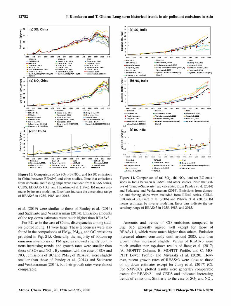
12782 J. Kurokawa and T. Ohara: Long-term historical trends in air pollutant emissions in Asia
Figure 10. Comparison of (a) SO2, (b) NOx , and (c) BC emissionsin China between REASv3 and other studies. Note that emissionsfrom domestic and fishing ships were excluded from REAS series,CEDS, EDGARv4.3.2, and Higashino et al. (1996). IM means esti-mates by inverse modeling. Error bars indicate the uncertainty rangeof REASv3 in 1955, 1985, and 2015.
et al. (2019) were similar to those of Pandey et al. (2014)and Sadavarte and Venkataraman (2014). Emission amountsof the top-down estimates were much higher than REASv3.
For BC, as in the case of China, discrepancies among stud-ies plotted in Fig. 11 were large. These tendencies were alsofound in the comparisons of PM10, PM2.5, and OC emissionsprovided in Fig. S15. Generally, the majority of bottom-upemission inventories of PM species showed slightly contin-uous increasing trends, and growth rates were smaller thanthose of SO2 and NOx . By contrast with the case of SO2 andNOx , emissions of BC and PM2.5 of REASv3 were slightlysmaller than those of Pandey et al. (2014) and Sadavarteand Venkataraman (2014), but their growth rates were almostcomparable.
Figure 11. Comparison of (a) SO2, (b) NOx , and (c) BC emis-sions in India between REASv3 and other studies. Note that val-ues of “Pandy+Sadavarte” are calculated from Pandey et al. (2014)and Sadavarte and Venkataraman (2014). Emissions from domes-tic and fishing ships were excluded from REAS series, CEDS,EDGARv4.3.2, Garg et al. (2006) and Paliwai et al. (2016). IMmeans estimates by inverse modeling. Error bars indicate the un-certainty range of REASv3 in 1955, 1985, and 2015.
Amounts and trends of CO emissions compared inFig. S15 generally agreed well except for those ofREASv1.1, which were much higher than others. Emissionincreased almost constantly until around 2005, and thengrowth rates increased slightly. Values of REASv3 weremuch smaller than top-down results of Jiang et al. (2017)(A: MOPITT Column, B: MOPITT Profile, and C: MO-PITT Lower Profile) and Miyazaki et al. (2020). How-ever, recent growth rates of REASv3 were close to thoseof top-down estimates except for Jiang et al. (2017) (C).For NMVOCs, plotted results were generally comparableexcept for REASv2.1 and CEDS and indicated increasingtrends of emissions. Similarly to the case of SO2 and NOx ,
Atmos. Chem. Phys., 20, 12761–12793, 2020 https://doi.org/10.5194/acp-20-12761-2020

J. Kurokawa and T. Ohara: Long-term historical trends in air pollutant emissions in Asia 12783
growth rates of REASv3 were smaller than those of Pandeyet al. (2014) and Sadavarte and Venkataraman (2014). ForNH3, a comparison of the emissions in Fig. S15 show sim-ilar increasing trends. Differences in emission amounts arealso relatively small, except for EDGARv4.3.2.
3.3.3 Other regions
Comparisons of emissions in Japan between REASv3 andother studies were provided in Fig. S16. For trends of SO2emissions in Japan, the majority of studies agreed with re-sults of REASv3 of rapid increases in the 1960s, keen de-creases in the 1970s, and gradually decreasing trends, exceptfor EDGARv4.3.2 and Streets et al. (2000), whose valueswere larger and smaller, respectively. For NOx , emissionsamounts of REASv3 were larger than those of most studiesespecially before 2000, except for CEDS (scaled to prelimi-nary historical data of REAS for Japan; Hoesly et al., 2018),Kannari et al. (2007), Zhang et al. (2009) based on Kannariet al. (2007) and Fukui et al. (2014). For PM species, the ma-jority of results in Fig. S16 agreed with decreasing trends ofREASv3 after 1990. On the other hand, emissions of BC andOC of CEDS increased almost monotonically until their peakaround 1990. These tendencies were much different fromREASv3. For CO, emission amounts of REASv3 were largerthan other results of especially REASv1, EDGARv4.3.2, andCEDS. However, after 2000, emissions and their decreas-ing trends of other studies were generally comparable withthose of REASv3. For NMVOCs, results of REASv3 after2000 generally agreed well with other studies which showedlarge decreasing trends, except for EDGARv4.3.2 and Zhanget al. (2009) based on Kannari et al. (2007). Trends ofNH3 emissions shown in Fig. S16 were similar except forEDGARv4.3.2 before the mid-1990s, which showed largergrowth rates. Emission amounts of REASv3 were smallerthan national inventories by Kannari et al. (2001) and Fukuiet al. (2014).
For SEA (see Fig. S17), increasing trends and amounts ofSO2 emissions of REASv3 agreed with other results exceptfor CEDS in the 1990s, Zhang et al. (2009), and Klimontet al. (2013). In CEDS, emissions decreased keenly duringthe late 1990s. A similar feature was also seen in REASv3,but its rate of decrease was much smaller. For NOx , all re-sults plotted in Fig. S17 indicated monotonically increasingtrends of emissions and agreed well until the early 2000s.After that, growth rates of REASv3 became larger thanEDGARv4.3.2 and smaller than CEDS (scaled to REASv2.1for SEA; Hoesly et al., 2018). For BC, REAS series andCEDS showed similar growth rates until around 2005. Onthe other hand, increasing rates of Klimont et al. (2017) andEDGARv4.3.2 after 1990 were much smaller and close tothose of REASv3 after 2005.
Most results of SO2 emissions in OEA in Fig. S18 showincreasing and decreasing trends from the late 1960s andthe early 1990s, respectively, although amounts in CEDS
from 1970 and 2000 were much smaller. For NOx , all resultsagreed well until the late 1980s, and REASv3, REASv1.1,and EDGARv4.3.2 showed similar increasing trends un-til around 2000. Emissions of CEDS became almost sta-ble after the late 1980s and started to decrease after 2005.The decreasing rates of REASv3 and CEDS are close after2005. On the other hand, emissions of EDGARv4.3.2 didnot change largely after around 2000. The similar tendencieswere shown in the case of SO2. BC emissions of REASv3and CEDS showed similar trends until 2000. Then, emissionsof REASv3 decreased almost monotonically, while thoseof CEDS were almost stable. Similarly, decreasing rates ofEDGARv4.3.2 after 2000 were much smaller than those ofREASv3.
For OSA, increasing trends and amounts of SO2 andNOx emissions were generally similar among studies plot-ted in Fig. S19. SO2 emissions of Streets et al. (2003a) andZhang et al. (2009) and NOx emissions of CEDS (scaledto REASv2.1; Hoesly et al., 2018) were higher than otherresults. For BC, discrepancies among studies were largerthan those of SO2 and NOx , but similar small monotonicallygrowth rates were shown in all results.
3.3.4 Relative ratios of emissions from each countryand region in Asia
Figure 12 compares trends of total emissions in Asia andrelative ratios of emissions from China, India, Japan, SEA,OEA, and OSA among REASv3, CEDS, and EDGARv4.3.2for SO2, NOx , and BC. Comparisons of other species arepresented in Fig. S20. From 1950 to the early 2000s, totalSO2 emissions in Asia of all inventories showed similar re-sults. For relative ratios, REASv3 and CEDS values weresimilar until the mid-2000s. Contributions from Japan wererelatively large from 1950 until around 1970 and then de-creased keenly. This was also found in EDGARv4.3.2, butthe rate of decrease was smaller than that of REASv3 andCEDS. Then, while emissions of REASv3 decreased largelyafter the mid-2000s, those of CDES and EDGARv4.3.2 con-tinued to increase. These discrepancies were mainly due todifferent trends of emissions from China. Actually, after themid-2000s, relative ratios of SO2 emissions in China werestable in CEDS and EDGARv4.3.2, but those in REASv3decreased significantly. Recently, increasing trends of rela-tive ratios of SO2 emissions in India are a common feature inREASv3, EDGARv4.3.2, and CEDS.
For NOx , Asia total emissions of REASv3 andEDGARv4.3.2 were close. Although emissions of CEDSwere larger than REASv3 and EDGARv4.3.2, trends weresimilar until early 2010. The different trends after 2010 be-tween REASv3 and CEDS were caused by those of emis-sions in China. For the contributing rates, REASv3 andCEDS generally showed similar temporal variations, al-though relative ratios of OSA were larger in CEDS. Contri-bution rates of Japan were large around 1970 and then grad-
https://doi.org/10.5194/acp-20-12761-2020 Atmos. Chem. Phys., 20, 12761–12793, 2020

12784 J. Kurokawa and T. Ohara: Long-term historical trends in air pollutant emissions in Asia
Figure 12. Comparison of trends of (a) SO2, (b) NOx , and (c) BC emissions in Asia and relative ratios of emissions from China, India, Japan,SEA, OEA, and OSA for (d, g, j) SO2, (e, h, k) NOx , and (f, i, l) BC among (d, e, f) REASv3, (g, h, i) CEDS, and (j, k. l) EDGARv4.3.2.Note that periods of CEDS and EDGARv4.3.2 shown here are during 1950–2014 and 1970–2012, respectively. See Fig. 1 for definitions ofSEA, OEA, and OSA.
ually decreased. Instead, those from China increased almostmonotonically until 2010. Similarly to the case of SO2, rela-tive ratios of China decreased recently in REASv3, but theywere almost stable in CEDS and EDGARv4.3.2. In addi-tion, contribution rates from India showed gradual increasingtrends in all the results.
For total Asia emissions of BC, trends of REASv3 andCEDS were similar until the late 1990s, but after 2000, whilegrowth rates of CEDS became larger, emissions of REASdid not change greatly and turned to decrease after 2010.Emission amounts and growth rates of EDGARv4.3.2 weresmaller than others until the mid-1990s, but after that thetrends were similar to those of REASv3. Compared to SO2and NOx , temporal variations of relative ratios of BC emis-sions from each country and regions were small in all the re-sults. In REASv3, contribution rates of Japan were large be-fore 1970 and then decreased afterwards. On the other hand,in CEDS, contribution rates of Japan after 1970 were largerthan those before 1970. After 2000, relative ratios of China inREASv3 were almost stable and showed a marginal decrease
after 2011. In CEDS and EDGARv4.3.2, contribution ratesof China increased during the first half of the 2000s and thenbecame almost stable. Similar tendencies were seen in OC.Compared to BC, relative ratios of China started to decreaseearlier only in REASv3.
For Asia total emissions of CO, although amounts ofCEDS were larger than others, trends of all results were closeuntil the early 2000s. After that, REASv3 showed large in-creases until 2010 and then started to decrease slightly. Thesetendencies were mainly controlled by emissions in China.Trends of the relative ratios were similar to those of BC,but contribution rates of China in REASv3 increased grad-ually until the mid-2000s and then decreased, while those inCEDS and EDGARv4.3.2 were almost stable. For NMVOCs,total emissions in Asia of REASv3 were smaller than others,but large increases in emissions were found from the early1990s. The corresponding feature was shown in contributionrates. Relative ratios of emissions from China in REASv3 in-creased largely during the 1990s and 2000s. Similar increas-ing trends were seen in EDGARv4.3.2, but growth rates of
Atmos. Chem. Phys., 20, 12761–12793, 2020 https://doi.org/10.5194/acp-20-12761-2020

J. Kurokawa and T. Ohara: Long-term historical trends in air pollutant emissions in Asia 12785
REASv3 were much larger. On the other hand, both tempo-ral variations and values of contribution rates of China wererelatively small in CEDS.
For NH3, trends of total emissions in Asia of REASv3were close to EDGARv4.3.2 and slightly larger than CEDSuntil around 2000. After that, growth rates of REASv3 wereclose to CEDS and those of EDGARv4.3.2 became larger.As a result, amounts of total Asia emissions of all invento-ries became almost the same after 2010. For relative ratiosof regions, contribution rates of China in REASv3 increasedgradually until the mid-2000s and then became almost stable,whereas those in CEDS and EDGARv4.3.2 show slightly de-creasing and increasing trends, respectively. In 2015, rela-tive ratios of NH3 emissions from China in REASv3 werebetween those of EDGARv4.3.2 and CEDS. Compared toEDGARv4.3.2 and CEDS, contribution rates of NH3 emis-sions from SEA region were relatively small in REASv3.
3.4 Uncertainty
In REASv3, uncertainties in emissions were estimated foreach country and region in 1955, 1985, and 2015 using basi-cally the same methodology as that of REASv2.1 (Kurokawaet al., 2013). First, uncertainties in all parameters used tocalculate emissions, such as activity data, emission factors,removal efficiencies, and sulfur contents of fuels, were esti-mated in the range of 2 %–150 %. In estimation of the uncer-tainties except for activity data, the following three causesneed to be considered: uncertainties in the data themselves,those caused by selections of the data, and those in settingsrelated to emission controls such as timing of introductionand penetration rates of abatement equipment. In this study,uncertainties in settings of emission controls were explicitlyconsidered only for removal efficiencies. The uncertaintiesin removal efficiencies were assumed to be zero for emissionsources where no emission controls were considered, whichmeans that uncertainties caused by neglecting emission con-trols were not considered. Furthermore, for emission sourceswhere introduction rates of abatement equipment were small,uncertainties caused by settings of emission controls were as-sumed to be small. Then, uncertainties in emissions from thepower plant, industry, road transport, other transport, domes-tic, and other sectors, as well as uncertainties in total emis-sions, were calculated for all the species. The uncertainties indifferent sub-sectors and activities were combined in quadra-ture assuming they were independent. On the other hand,for uncertainties in national emissions in China, India, andJapan, those in their sub-regions were added linearly. De-tails of the methodology and settings of uncertainties in eachcomponent were described in Sect. S10 of the Supplement.Similarly to REASv2.1, uncertainties in emissions that werenot originally developed in REASv3 (NH3 emissions frommanure management and fertilizer application, and NMVOCevaporative emissions from Japan and the Republic of Korea)were not evaluated in this study.
Table 4 summarizes the estimated uncertainties in totalemissions of each species for China, India, Japan, SEA,OEA, and OSA in 1955, 1985, and 2015. Uncertainties inemissions from each sector were provided in the Supplementtables (Table S1 for SO2, NOx , CO, CO2, PM10, PM2.5, BC,and OC, Table S2 for NMVOCs, and Table S3 for NH3).For most regions and years, uncertainties for SO2, NOx , andCO2 are smaller than other species. Major emission sourcesof these species are power plants and large industry sectors.Uncertainties in activity data of these species were assumedto be small because power plants and large industries are crit-ically important for each country and related statistics are ex-pected to be accurate. In addition, uncertainties in emissionfactors of combustion at high temperature in power plantsand large industries are considered to be small. For SO2emissions in China, uncertainties in 2015 were estimated tobe slightly larger than those in 1985 due to uncertainties forremoval efficiencies which were not considered in 1985. Thesame situation was found in uncertainties in NOx emissionsfrom power plants in China between 1985 and 2015. Lackof detailed information for changes in technologies such ascombustion burners and abatement equipment affects uncer-tainties in recent emission trends in Asia. For South andSoutheast Asia, uncertainties in SO2 emissions in 1985 wereslightly smaller than those in 2015. This is because settingsof sulfur contents in fuels were based on surveys conductedin 1990 (Kato and Akimoto, 1992), and thus the uncertaintiesin 1985 were assumed to be smaller than those in 2015. InREASv3, information on temporal variations of sulfur con-tents in fuels both by changes in fuel properties and by low-sulfur fuel regulations was limited, which were also causes ofuncertainties in emission trends. In general, uncertainties inemissions in REASv3 were smaller in recent years becauseactivity data of recent years are more accurate. However, de-tailed surveys for recent changes in technologies and infor-mation on emission controls are essential in future studies.
On the other hand, uncertainties in PM species are largecompared to other species for most regions and years. Formost countries in Asia, the majority of their emissions werefrom combustion at relatively low temperatures in small in-dustries and residential sectors. Accuracies of activity dataand emission factors for these sources are assumed to be low,especially for biofuel combustion. Therefore, uncertainties inOC emissions, mainly from biofuel combustion in Asia, arethe largest for most regions and years. Uncertainties in PM10are generally smaller than other PM species. This is becausefor PM10 emissions, contribution rates of power plants andindustry sectors are generally larger than those of other PMspecies. For CO and NMVOCs, in general, uncertainties inemission factors are assumed to be greater than SO2, NOx ,and CO2 but smaller than PM2.5, BC, and OC. Therefore,uncertainties in total CO and NMVOC emissions are gener-ally between those of other species. For Southeast and SouthAsia, uncertainties in CO and NMVOCs are comparable with
https://doi.org/10.5194/acp-20-12761-2020 Atmos. Chem. Phys., 20, 12761–12793, 2020
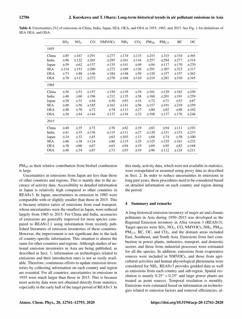
12786 J. Kurokawa and T. Ohara: Long-term historical trends in air pollutant emissions in Asia
Table 4. Uncertainties [%] of emissions in China, India, Japan, SEA, OEA, and OSA in 1955, 1985, and 2015. See Fig. 1 for definitions ofSEA OEA, and OSA.
SO2 NOx CO NMVOCs NH3 CO2 PM10 PM2.5 BC OC
1955
China ±85 ±167 ±291 ±277 ±174 ±133 ±253 ±315 ±334 ±365India ±96 ±122 ±265 ±295 ±161 ±116 ±257 ±294 ±277 ±314Japan ±59 ±62 ±157 ±135 ±141 ±49 ±94 ±117 ±170 ±270SEA ±134 ±153 ±260 ±272 ±169 ±126 ±291 ±307 ±323 ±317OEA ±73 ±88 ±146 ±184 ±148 ±59 ±120 ±157 ±157 ±262OSA ±70 ±112 ±272 ±270 ±168 ±110 ±219 ±281 ±310 ±345
1985
China ±36 ±53 ±157 ±150 ±139 ±39 ±101 ±129 ±182 ±250India ±40 ±60 ±196 ±212 ±135 ±58 ±160 ±201 ±191 ±259Japan ±30 ±31 ±44 ±50 ±93 ±14 ±72 ±71 ±53 ±67SEA ±40 ±56 ±185 ±162 ±141 ±56 ±157 ±191 ±218 ±259OEA ±48 ±70 ±72 ±78 ±113 ±27 ±80 ±82 ±88 ±102OSA ±36 ±44 ±144 ±137 ±134 ±33 ±108 ±137 ±176 ±248
2015
China ±40 ±35 ±73 ±76 ±82 ±19 ±83 ±94 ±111 ±193India ±41 ±35 ±136 ±115 ±111 ±27 ±120 ±151 ±133 ±233Japan ±34 ±32 ±45 ±63 ±103 ±13 ±68 ±74 ±58 ±100SEA ±46 ±38 ±124 ±86 ±115 ±25 ±125 ±155 ±161 ±232OEA ±38 ±60 ±67 ±63 ±94 ±19 ±69 ±85 ±82 ±168OSA ±40 ±34 ±87 ±73 ±93 ±19 ±96 ±112 ±124 ±211
PM10 as their relative contribution from biofuel combustionis large.
Uncertainties in emissions from Japan are less than thoseof other countries and regions. This is mainly due to the ac-curacy of activity data. Accessibility to detailed informationin Japan is relatively high compared to other countries inREASv3. In Japan, uncertainties in emission in 1985 werecomparable with or slightly smaller than those in 2015. Thisis because relative ratios of emissions from road transport,whose uncertainties were the smallest in Japan, were reducedlargely from 1985 to 2015. For China and India, accuraciesof emissions are generally improved for most species com-pared to REASv2.1 using information from recently pub-lished literatures of emission inventories of these countries.However, the improvement is not significant due to the lackof country-specific information. This situation is almost thesame for other countries and regions. Although studies of na-tional emission inventories in Asia are being published, asdescribed in Sect. 1, information on technologies related toemissions and their introduction rates is not as easily avail-able. Therefore, continuous efforts to update emission inven-tories by collecting information on each country and regionare essential. For all countries, uncertainties in emissions in1955 were much larger than those in 2015. This is becausemost activity data were not obtained directly from statistics,especially in the early half of the target period of REASv3. In
this study, activity data, which were not available in statistics,were extrapolated or assumed using proxy data as describedin Sect. 2. In order to reduce uncertainties in emissions inlong past years, these procedures need to be considered basedon detailed information on each country and region duringthe period.
4 Summary and remarks
A long historical emission inventory of major air and climatepollutants in Asia during 1950–2015 was developed as theRegional Emission inventory in ASia version 3 (REASv3).Target species were SO2, NOx , CO, NMVOCs, NH3, PM10,PM2.5, BC, OC, and CO2, and the domain areas includedEast, Southeast, and South Asia. Emissions from fuel com-bustion in power plants, industries, transport, and domesticsectors and those from industrial processes were estimatedfor all the species. In addition, emissions from evaporativesources were included in NMVOCs, and those from agri-cultural activities and human physiological phenomena wereconsidered for NH3. REASv3 provides gridded data as wellas emissions from each country and sub-region. Spatial res-olution is mainly 0.25◦× 0.25◦ and large power plants aretreated as point sources. Temporal resolution is monthly.Emissions were estimated based on information on technolo-gies related to emission factors and removal efficiencies, al-
Atmos. Chem. Phys., 20, 12761–12793, 2020 https://doi.org/10.5194/acp-20-12761-2020

J. Kurokawa and T. Ohara: Long-term historical trends in air pollutant emissions in Asia 12787
though available data and literatures are limited in the case ofAsia. Activity data for recent years were collected from inter-national and national statistics, and those of past years, whendetailed information was not available, were extrapolated us-ing proxy data for the target period of REASv3. Details ofmethodologies such as data sources and treatments, settingsof emission factors and emission controls, and related as-sumptions were provided in the Supplement document en-titled “Supplementary information and data to methodologyof REASv3”.
Total emissions in Asia averaged during 1950–1955 and2010–2015 (growth rates in these 60 years estimated fromthe two averages) are SO2: 3.2 Tg, 42.4 Tg (13.1); NOx :1.6 Tg, 47.3 Tg (29.1); CO: 56.1 Tg, 303 Tg (5.4); NMVOCs:7.0 Tg, 57.8 Tg (8.3); NH3: 8.0 Tg, 31.3 Tg (3.9); CO2:1.1 Pg, 18.6 Pg (16.5); PM10: 5.9 Tg, 30.2 Tg (5.1); PM2.5:4.6 Tg, 21.3 Tg (4.6); BC: 0.69 Tg, 3.2 Tg (4.7); and OC:2.5 Tg, 6.6 Tg (2.7). Clearly, all the air pollutant emissionsin Asia increased significantly during these 6 decades. How-ever, situations were different among countries and regions.In recent years, the relative contribution of air pollutant emis-sions from China was the largest along with rapid increasein economic growth, but most species have reached theirpeaks, and the growth rates of other species have becomeat least small or almost zero. For SO2 and NOx , introduc-tion of abatement equipment, especially for coal-fired powerplants such as FGD and SCR were considered to be effec-tive in reducing emissions. For PM species, in addition tocontrol equipment in industrial plants, emissions decreasedrecently due to reduced usage of biofuels. On the other hand,air pollutant emissions from India showed an almost contin-uous increase. Growth rates were larger for SO2 and NOx ,but their structures of emissions were different. Large partsof SO2 emissions were obtained from coal combustion inpower plants and the industrial sector, and the recent rapidincrease in SO2 emission was mainly from coal-fired powerplants. For NOx , contribution from road transport especiallydiesel vehicles were almost comparable with those of powerplants. For PM species, the majority of emissions were fromthe residential sector in the 1950s–1960s, and its contributionis still considered to be large. Recent increasing trends weremainly caused by emissions from power and industrial plantsand road vehicles. Trends in Japan were much different thanthose of the whole of Asia. Emissions increased rapidly alongwith economic growth during the 1950s–1970s, but those ofmost species were reduced largely from peak values. In ad-dition, peak years were mostly 40 years ago, reflecting thetime series of introduction of control measures to mitigateair pollution. Similar features were found in the Republic ofKorea and Taiwan. For other countries in Asia, emissions ofair pollutants generally showed increasing trends along witheconomic situation and motorization. As described above,trends and spatial distribution of air pollutants in Asia arenot simple and are becoming complicated.
Mitigation of air and climate pollutant emissions is an ur-gent issue in most Asian countries, but the situation is dif-ferent country-wise. In this study, detailed discussion on ef-fects of emission controls was conducted only for China andJapan due to limitation of information. Therefore, continuousefforts to develop and update emission inventories in Asiabased on country-specific information are essential, espe-cially for countries and regions other than China and Japan.On the other hand, there are inevitable uncertainties in pa-rameters required to develop emission inventories, such asactivity data and emission factors. In addition, it is funda-mentally impossible to develop a real-time emission inven-tory because there is a time lag in the publication of ba-sic statistics essential to estimate emissions. Recently, satel-lite observation data of air pollutants have become availableat a finer scale for many species, such as NOx , SO2, andNH3. Evaluations and improvements of REASv3 based onthese data as well as results of modeling studies, such as in-verse modeling, are more important next steps. Also, addi-tion of target species, especially CH4, which is one of the keyspecies in mitigating both air pollution and global warming,is another important task for future studies.
Data availability. Monthly gridded emission data sets at 0.25◦×0.25◦ resolution for major sectors and emission table data for ma-jor sectors and fuel types in each country and region during 1950–2015 developed in this study are available from https://www.nies.go.jp/REAS/index.html#REASv3.2 (Kurokawa and Ohara, 2020)in a data download site of REAS (https://www.nies.go.jp/REAS/index.html, last access: 31 October 2020). Note that data setsof REASv3.1 were released after a publication of Kurokawa etal. (2019) from December 2019. The data sets were revised andthe updated data are available as REASv3.2 together with a publi-cation of this paper. Differences between REASv3.2 and REASv3.1were presented and discussed in the Supplement document entitled“Differences between REASv3.2 and REASv3.1”.
Supplement. The supplement related to this article is available on-line at: https://doi.org/10.5194/acp-20-12761-2020-supplement.
Author contributions. JK and TO conducted the study design. JKcontributed to actual works for development of REASv3 such ascollecting data and information, settings of parameters, calculat-ing emissions, and creating final data sets. JK and TO analyzedand discussed the estimated emissions in REASv3. JK prepared themanuscript with contributions from TO.
Competing interests. The authors declare that they have no conflictof interest.
Acknowledgements. We appreciate Kazumasa Kawashima (Mit-subishi UFJ Research and Consulting Co., Ltd.) and Tetsuo Fukui
https://doi.org/10.5194/acp-20-12761-2020 Atmos. Chem. Phys., 20, 12761–12793, 2020

12788 J. Kurokawa and T. Ohara: Long-term historical trends in air pollutant emissions in Asia
(The Institute of Behavioral Sciences) for their great support incollecting activity data and survey information for settings of pa-rameters. We acknowledge Keiya Yumimoto (Kyushu University),Syuichi Itahashi (Central Research Institute of Electric Power In-dustry), Tatsuya Nagashima (National Institute for EnvironmentalStudies), and Takashi Maki (Meteorological Research Institute) fortheir valuable suggestions to improve REAS. We are grateful toDaisuke Goto (National Institute for Environmental Studies) forhis support to update the data download site of REAS. We thankYusuke Kiriyama (Asia Center for Air Pollution Research) for hishelp in drawing figures of gridded emission maps.
Financial support. This research has been supported by the En-vironmental Research and Technology Development Fund (grantno. S-12) of the Environmental Restoration and ConservationAgency of Japan and the Japan Society for the Promotion of Sci-ence, KAKENHI (grant no. 19K12303).
Review statement. This paper was edited by Qiang Zhang and re-viewed by two anonymous referees.
References
Baidya, S. and Borken-Kleefeld, J.: Atmospheric emissions fromroad transportation in India, Energy Policy, 37, 3812–3822,https://doi.org/10.1016/j.enpol.2009.07.010, 2009.
Bond, T. C., Streets, D. G., Yarber, K. F., Nelson, S. M., Woo, J.-H.,and Klimont, Z.: A technology-based global inventory of blackand organic carbon emissions from combustion, J. Geophys.Res., 109, D14203, https://doi.org/10.1029/2003JD003697,2004.
Chandramouli, C.: Census of India 2011, Tables on Houses, House-hold Amenities and Assets, the Indian Administrative ServiceRegistrar General & Census Commissioner, India, 2011.
Chatani, S., Yamaji, K., Sakurai, T., Itahashi, S., Shi-madera, H., Kitayama, K., and Hayami, H.: Overview ofmodel inter-comparison in Japan’s Study for ReferenceAir Quality Modeling (J-STREAM), Atmosphere, 9, 19,https://doi.org/10.3390/atmos9010019, 2018.
Clean Air Asia: Accessing Asia: Air Pollution and Greenhouse GasEmissions Indicators for Road Transport and Electricity, PasingCity, Philippines, 2012.
Clean Air Asia: Developments in the Asia-Pacific Region, the 10thGlobal Partnership Meeting of the Partnership for Clean Fuelsand Vehicles, 13 May 2014, Paris, 2014.
Crippa, M., Janssens-Maenhout, G., Dentener, F., Guizzardi, D.,Sindelarova, K., Muntean, M., Van Dingenen, R., and Granier,C.: Forty years of improvements in European air quality: re-gional policy-industry interactions with global impacts, Atmos.Chem. Phys., 16, 3825–3841, https://doi.org/10.5194/acp-16-3825-2016, 2016.
Ding, J., Miyazaki, K., van der A, R. J., Mijling, B., Kurokawa,J.-I., Cho, S., Janssens-Maenhout, G., Zhang, Q., Liu, F.,and Levelt, P. F.: Intercomparison of NOx emission invento-ries over East Asia, Atmos. Chem. Phys., 17, 10125–10141,https://doi.org/10.5194/acp-17-10125-2017, 2017.
EEA (European Environment Agency): EMEP/EEA air pol-lutant emission inventory guidebook 2016, EEA Report,21, available at: https://www.eea.europa.eu/publications/emep-eea-guidebook-2016 (last access: 1 August 2020), 2016.
Fukui, T., Kokuryo, K., Baba, T., and Kannari, A.: UpdatingEAGrid2000-Japan emissions inventory based on the recentemission trends (in Japanese), J. Jpn. Soc. Atmos. Environ., 49,117–125, https://doi.org/10.11298/taiki.49.117, 2014.
Garg, A., Shukla, P. R., Bhattacharaya, S., and Dadhwal, V. K.:Sub-region (district) and sector level SO2 and NOx emissionsfor India: assessment of inventories and mitigation flexibility,Atmos. Environ., 35, 703–713, https://doi.org/10.1016/S1352-2310(00)00316-2, 2001.
Garg, A., Shukla, P. R., and Kaphe, M.: The sectoral trends of multi-gas emissions inventory of India, Atmos. Environ., 40, 4608–4620, https://doi.org/10.1016/j.atmosenv.2006.03.045, 2006.
Goto, S: Progress of non-ferrous metal smelting in re-cent 10 years, J. Jpn. Mining Ind. Assoc., 97, 602–608,https://doi.org/10.2473/shigentosozai1953.97.1122_602, 1981(in Japanese).
Guttikunda, S. K. and Jawahar, P.: Atmospheric emis-sions and pollution from the coal-fired thermalpower plants in India, Atmos. Environ., 92, 449–460,https://doi.org/10.1016/j.atmosenv.2014.04.057, 2014.
Hao, J., Tian, H., and Lu, Y.: Emission Inventories ofNOx from Commercial Energy Consumption in China,1995–1998, Environ. Sci. Technol., 36, 552–560,https://doi.org/10.1021/es015601k, 2002.
He, K., Huo, H., Zhang, Q., He, D., An, F., Wang, M.,and Walsh, M. P.: Oil consumption and CO2 emissionsin China’s road transport: current status, future trends,and policy implications, Energy Policy, 33, 1499–1507,https://doi.org/10.1016/j.enpol.2004.01.007, 2005.
Higashino, H., Tonooka, Y., Yanagisawa, Y., and Ikeda, Y.: Emis-sion inventory of air pollutants in East Asia – Anthropogenicemissions of sulfur dioxide in China, J. Jpn. Soc. Atmos., 30,374–390, https://doi.org/10.11298/taiki1995.30.6_374, 1995 (inJapanese).
Higashino, H., Tonooka, Y., Yanagisawa, Y., and Ikeda, Y.: Emis-sion inventory of air pollutants in East Asia (II) – Focused onestimation of NOx and CO2 emissions in China, J. Jpn. Soc. At-mos., 31, 262–281, https://doi.org/10.11298/taiki1995.31.6_262,1996 (in Japanese).
Hoesly, R. M., Smith, S. J., Feng, L., Klimont, Z., Janssens-Maenhout, G., Pitkanen, T., Seibert, J. J., Vu, L., Andres, R.J., Bolt, R. M., Bond, T. C., Dawidowski, L., Kholod, N.,Kurokawa, J.-I., Li, M., Liu, L., Lu, Z., Moura, M. C. P.,O’Rourke, P. R., and Zhang, Q.: Historical (1750–2014) anthro-pogenic emissions of reactive gases and aerosols from the Com-munity Emissions Data System (CEDS), Geosci. Model Dev., 11,369–408, https://doi.org/10.5194/gmd-11-369-2018, 2018.
Hua, S., Tian. H., Wang, K., Zhu, C., Gao, J., Ma, Y., Xue,Y., Wang, Y., Duan, S., and Zhou, J.: Atmospheric emis-sion inventory of hazardous air pollutants from China’s ce-ment plants: Temporal trends, spatial variation characteris-tics and scenario projections, Atmos. Environ., 128, 1–9,https://doi.org/10.1016/j.atmosenv.2015.12.056, 2016.
Huo, H., Lei, Y., Zhang, Q., Zhao, L., and He, K.: China’scoke industry: Recent policies, technology shift, and implica-
Atmos. Chem. Phys., 20, 12761–12793, 2020 https://doi.org/10.5194/acp-20-12761-2020

J. Kurokawa and T. Ohara: Long-term historical trends in air pollutant emissions in Asia 12789
tion for energy and the environment, Energy Policy, 51, 397–404,https://doi.org/10.1016/j.enpol.2012.08.041, 2012a.
Huo, H., Zhang, Q., He, K., Yao, Z., and Wang, M.: Vehicle-useintensity in China: Current status and future trend, Energy Policy,43, 6–16, https://doi.org/10.1016/j.enpol.2011.09.019, 2012b.
IEA (International Energy Agency): World Energy Balances, IEA,Paris, 2017.
IPCC (Intergovernmental Panel on Climate Change): the NationalGreenhouse Gas Inventories Programme, edited by: Eggleston,H. S., Buendia, L., Miwa, K., Ngara, T., and Tanabe, K.,2006 IPCC Guidelines for National Greenhouse Gas Inventories,published by the Institute for Global Environmental Strategies(IGES), Hayama, Japan on behalf of the IPCC, available at: http://www.ipcc-nggip.iges.or.jp/public/2006gl/index.html (last ac-cess: 1 August 2020), 2006.
IRF (International Road Federation): World Road Statistics 1963–2015, International Road Federation, Geneva, 1990–2018.
Itahashi, S., Yumimoto, K., Kurokawa, J., Morino, Y., Nagashima,T., Miyazaki, K., Maki, T., and Ohara, T.: Inverse estimationof NOx emissions over China and India 2005–2016: contrast-ing recent trends and future perspectives, Environ. Res. Lett., 14,124020, https://doi.org/10.1088/1748-9326/ab4d7f, 2019.
Janssens-Maenhout, G., Crippa, M., Guizzardi, D., Dentener, F.,Muntean, M., Pouliot, G., Keating, T., Zhang, Q., Kurokawa,J., Wankmüller, R., Denier van der Gon, H., Kuenen, J. J.P., Klimont, Z., Frost, G., Darras, S., Koffi, B., and Li,M.: HTAP_v2.2: a mosaic of regional and global emissiongrid maps for 2008 and 2010 to study hemispheric trans-port of air pollution, Atmos. Chem. Phys., 15, 11411–11432,https://doi.org/10.5194/acp-15-11411-2015, 2015.
Japan Environmental Sanitation Center and Suuri Keikaku: Reportfor prevention of air pollution in East Asia Annex I: Emissioninventory in Vietnam and policy analysis for prevention of airpollution, 2011 (in Japanese).
Japan Statistical Association: Historical Statistics of Japan NewEdition Volume 3, Statistics Bureau, Ministry of Internal Affairsand Communications, 2006.
Jayarathne, T., Stockwell, C. E., Bhave, P. V., Praveen, P. S., Rath-nayake, C. M., Islam, Md. R., Panday, A. K., Adhikari, S., Ma-harjan, R., Goetz, J. D., DeCarlo, P. F., Saikawa, E., Yokel-son, R. J., and Stone, E. A.: Nepal Ambient Monitoring andSource Testing Experiment (NAMaSTE): emissions of particu-late matter from wood- and dung-fueled cooking fires, garbageand crop residue burning, brick kilns, and other sources, At-mos. Chem. Phys., 18, 2259–2286, https://doi.org/10.5194/acp-18-2259-2018, 2018.
Jiang, Z., Worden, J. R., Worden, H., Deeter, M., Jones, D. B.A., Arellano, A. F., and Henze, D. K.: A 15-year record ofCO emissions constrained by MOPITT CO observations, At-mos. Chem. Phys., 17, 4565–4583, https://doi.org/10.5194/acp-17-4565-2017, 2017.
JPEC (Japan Petroleum Energy Center): Emission inventory of roadtransport in Japan, JPEC Technical Report, JPEC-2011AQ-02-06, 136 pp., 2012a (in Japanese).
JPEC: Emission inventory of sources other than road transport inJapan, JPEC Technical Report, JPEC-2011AQ-02-07, 288 pp.,2012b (in Japanese).
JPEC: Speciation profiles of VOC, PM, and NOx emissions for at-mospheric simulations of PM2.5, JPEC Technical Report, JPEC-2011AQ-02-08, 69 pp., 2012c (in Japanese).
JPEC: Emission inventory of PM2.5 and profiles of emissionsources, Report of Ministry of Environment of Japan, 2014.
Kang, Y., Liu, M., Song, Y., Huang, X., Yao, H., Cai, X., Zhang,H., Kang, L., Liu, X., Yan, X., He, H., Zhang, Q., Shao, M.,and Zhu, T.: High-resolution ammonia emissions inventories inChina from 1980 to 2012, Atmos. Chem. Phys., 16, 2043–2058,https://doi.org/10.5194/acp-16-2043-2016, 2016.
Kannari, A., Baba, T, and Hayami, H.: Estimation of ammoniaemissions in Japan (in Japanese), J. Jpn. Soc. Atmos. Environ.,36, 29–38, https://doi.org/10.11298/taiki1995.36.29, 2001.
Kannari, A., Tonooka, Y., Baba, T., and Murano, K.: Develop-ment of multiple-species 1 km× 1 km resolution hourly basisemissions inventory for Japan, Atmos. Environ., 41, 3428–3439,https://doi.org/10.1016/j.atmosenv.2006.12.015, 2007.
Kato, N. and Akimoto, H.: Anthropogenic emissions of SO2 andNOx in Asia: emissions inventories, Atmos. Environ., 26, 2997–3017, https://doi.org/10.1016/0960-1686(92)90291-R, 1992.
Klein Goldewijk, K., Beusen, A., Doelman, J., and Stehfest, E.: An-thropogenic land use estimates for the Holocene – HYDE 3.2,Earth Syst. Sci. Data, 9, 927–953, https://doi.org/10.5194/essd-9-927-2017, 2017.
Klimont, Z., Cofala, J., Bertok, I., Amann, M., Heyes, C., andGyarfas, F.: Modeling particulate emissions in Europe: A frame-work to estimate reduction potential and control costs, IIASA,Interim Report IR-02-076, 2002.
Klimont, Z., Smith, S. J., and Cofala, J.: The last decade ofglobal anthropogenic sulfur dioxide: 2000–2011 emissions,Environ. Res., Lett., 8, 014003, https://doi.org/10.1088/1748-9326/8/1/014003, 2013.
Klimont, Z., Kupiainen, K., Heyes, C., Purohit, P., Cofala, J., Rafaj,P., Borken-Kleefeld, J., and Schöpp, W.: Global anthropogenicemissions of particulate matter including black carbon, Atmos.Chem. Phys., 17, 8681–8723, https://doi.org/10.5194/acp-17-8681-2017, 2017.
Kupiainen, K. and Klimont, Z.: Primary emissions of submicronand carbonaceous particles in Europe and the potential for theircontrol, IIASA, Interim Report IR-04-079, 2004.
Kurokawa, J. and Ohara, T.: Long-term historical trends in air pol-lutant emissions in Asia: Regional Emission inventory in ASia(REAS) version 3, available at: https://www.nies.go.jp/REAS/index.html#REASv3.2 (last access: 31 October 2020), 2020.
Kurokawa, J., Ohara, T., Morikawa, T., Hanayama, S., Janssens-Maenhout, G., Fukui, T., Kawashima, K., and Akimoto, H.:Emissions of air pollutants and greenhouse gases over Asian re-gions during 2000–2008: Regional Emission inventory in ASia(REAS) version 2, Atmos. Chem. Phys., 13, 11019–11058,https://doi.org/10.5194/acp-13-11019-2013, 2013.
Lee, D.-G., Lee, Y.-M., Jang, K.-W., Yoo, C., Kang, K.-H., Lee, J.-H., Jung, S.-W., Park, J.-M., Lee, S.-B., Han, J.-S., Hong, J.-H.,and Lee, S.-J.: Korean national emissions inventory system and2007 air pollutant emissions, Asian J. Atmos. Environ., 5, 278–291, https://doi.org/10.5572/ajae.2011.5.4.278, 2011.
Lei, Y., Zhang, Q., He, K. B., and Streets, D. G.: Primary anthro-pogenic aerosol emission trends for China, 1990–2005, Atmos.Chem. Phys., 11, 931–954, https://doi.org/10.5194/acp-11-931-2011, 2011.
https://doi.org/10.5194/acp-20-12761-2020 Atmos. Chem. Phys., 20, 12761–12793, 2020

12790 J. Kurokawa and T. Ohara: Long-term historical trends in air pollutant emissions in Asia
Li, M., Zhang, Q., Streets, D. G., He, K. B., Cheng, Y. F., Em-mons, L. K., Huo, H., Kang, S. C., Lu, Z., Shao, M., Su, H.,Yu, X., and Zhang, Y.: Mapping Asian anthropogenic emis-sions of non-methane volatile organic compounds to multiplechemical mechanisms, Atmos. Chem. Phys., 14, 5617–5638,https://doi.org/10.5194/acp-14-5617-2014, 2014.
Li, M., Zhang, Q., Kurokawa, J.-I., Woo, J.-H., He, K., Lu, Z.,Ohara, T., Song, Y., Streets, D. G., Carmichael, G. R., Cheng,Y., Hong, C., Huo, H., Jiang, X., Kang, S., Liu, F., Su, H.,and Zheng, B.: MIX: a mosaic Asian anthropogenic emissioninventory under the international collaboration framework ofthe MICS-Asia and HTAP, Atmos. Chem. Phys., 17, 935–963,https://doi.org/10.5194/acp-17-935-2017, 2017a.
Li, M., Liu, H., Geng, G., Hong, C., Liu, F., Song, Y., Tong, D.,Zheng, B., Cui, H., Man, H., Zhang, Q., and He, K.: Anthro-pogenic emission inventories in China: a review, National Sci-ence Review, 4, 834–866, https://doi.org/10.1093/nsr/nwx150,2017b.
Li, C., McLinden, C., Fioletov, V., Krotkov, N., Carn, S.,Joiner, J., Streets, D., He, H., Ren, X., Li, Z., and Dick-erson, R.: India is overtaking China as the world’s largestemitter of anthropogenic sulfur dioxide, Sci. Rep., 7, 14304,https://doi.org/10.1038/s41598-017-14639-8, 2017.
Liu, F., Zhang, Q., Tong, D., Zheng, B., Li, M., Huo, H.,and He, K. B.: High-resolution inventory of technologies, ac-tivities, and emissions of coal-fired power plants in Chinafrom 1990 to 2010, Atmos. Chem. Phys., 15, 13299–13317,https://doi.org/10.5194/acp-15-13299-2015, 2015.
Lu, Z., Streets, D. G., Zhang, Q., Wang, S., Carmichael, G.R., Cheng, Y. F., Wei, C., Chin, M., Diehl, T., and Tan,Q.: Sulfur dioxide emissions in China and sulfur trends inEast Asia since 2000, Atmos. Chem. Phys., 10, 6311–6331,https://doi.org/10.5194/acp-10-6311-2010, 2010.
Lu, Z., Zhang, Q., and Streets, D. G.: Sulfur dioxide andprimary carbonaceous aerosol emissions in China andIndia, 1996–2010, Atmos. Chem. Phys., 11, 9839–9864,https://doi.org/10.5194/acp-11-9839-2011, 2011.
Ma, Q., Cai, S., Wang, S., Zhao, B., Martin, R. V., Brauer, M., Co-hen, A., Jiang, J., Zhou, W., Hao, J., Frostad, J., Forouzanfar,M. H., and Burnett, R. T.: Impacts of coal burning on ambientPM2.5 pollution in China, Atmos. Chem. Phys., 17, 4477–4491,https://doi.org/10.5194/acp-17-4477-2017, 2017.
Maithel, S.: Evaluating energy conservation potential of brick pro-duction in India, Greentech Knowledge Solutions Pvt Ldt., NewDelhi, 2013.
Maithel, S., Lalchandani, D., Malhotra, G., Bhanware, P., Uma,R., Ragavan, S., Athalye, V., Bindiy, K. R., Reddy, S., Bond,T, Weyant, C., Baum, E., Kim Thoa, V. T., Thu Phuong, N.,and Kim Thanh, T.: Brick Kilns performance assessment: ARoadmap for Cleaner Brick Production in India, Shakti Sustain-able Energy Foundation and Climate Works Foundation Sup-ported Initiative, New Delhi, 2012.
Malla, S.: Assessment of mobility and its impact on en-ergy use and air pollution in Nepal, Energy, 69, 485–496,https://doi.org/10.1016/j.energy.2014.03.041, 2014.
METI (Ministry of Economy Trade and Industry of Japan): Reportsof Pollutants Release and Transfer Register (2001–2015), Chem-ical Management Policy Division, 2003–2017 (in Japanese).
Mitchell, B. R.: International historical statistics: Africa, Asia &Oceania, 1750–1993 3rd ed., Macmillan reference Ldt., 1998.
Mishra, D. and Goyal, P.: Estimation of vehicularemissions using dynamic emission factors: A casestudy of Delhi, India, Atmos. Environ., 98, 1–7,https://doi.org/10.1016/j.atmosenv.2014.08.047, 2014.
Miyazaki, K., Bowman, K., Sekiya, T., Eskes, H., Boersma, F., Wor-den, H., Livesey, N., Payne, V. H., Sudo, K., Kanaya, Y., Taki-gawa, M., and Ogochi, K.: Updated tropospheric chemistry re-analysis and emission estimates, TCR-2, for 2005–2018, EarthSyst. Sci. Data, 12, 2223–2259, https://doi.org/10.5194/essd-12-2223-2020, 2020.
MLTI (Ministry of Land, Infrastructure, Transport and Tourism ofJapan): Annual Report of Road Statistics (1960–2015), Informa-tion Policy Division, 1961–2016 (in Japanese).
MOEJ (Ministry of Environment of Japan): Report on Volatile Or-ganic Compound (VOC) Emission Inventory Compiled, avail-able at: http://www.env.go.jp/air/osen/voc/inventory.html (lastaccess: 1 August 2020), 2017 (in Japanese).
MRI (Mitsubishi Research Institute): Survey report for technologiesused to overcome industrial air pollution in Japan, Environment& Energy Research Division, Mitsubishi Research Institute, Inc.,2015 (in Japanese).
National Bureau of Statistics of China: China Statistical Yearbook(1985–2015), China Statistics Press, Beijing, 1986–2016.
National Bureau of Statistics of China: China Energy StatisticalYearbook (1985; 1995–2015), China Statistics Press, Beijing,1986, 2001–2017.
Nishina, K., Ito, A., Hanasaki, N., and Hayashi, S.: Reconstructionof spatially detailed global map of NH+4 and NO−3 applicationin synthetic nitrogen fertilizer, Earth Syst. Sci. Data, 9, 149–162,https://doi.org/10.5194/essd-9-149-2017, 2017.
Ohara, T., Akimoto, H., Kurokawa, J., Horii, N., Yamaji, K., Yan,X., and Hayasaka, T.: An Asian emission inventory of anthro-pogenic emission sources for the period 1980–2020, Atmos.Chem. Phys., 7, 4419–4444, https://doi.org/10.5194/acp-7-4419-2007, 2007.
Paliwal, U., Sharma, M., and Burkhart, J. F.: Monthly and spa-tially resolved black carbon emission inventory of India: un-certainty analysis, Atmos. Chem. Phys., 16, 12457–12476,https://doi.org/10.5194/acp-16-12457-2016, 2016.
Pandey, A. and Venkataraman, C.: Estimating emissions fromthe Indian transport sector with on-road fleet composi-tion and traffic volume, Atmos. Environ., 98, 123–133,https://doi.org/10.1016/j.atmosenv.2014.08.039, 2014.
Pandey, A., Sadavarte, P., Rao, A. B., and Venkataraman,C.: Trends in multi-pollutant emissions from a technology-linked inventory for India: II. Residential, agricultural andinformal industry sectors, Atmos. Environ., 99, 341–352,https://doi.org/10.1016/j.atmosenv.2014.09.080, 2014.
Permadi D. A., Sofyan, A., and Oanh, N. T. K.: Assess-ment of emissions of greenhouse gases and air pollutantsin Indonesia and impacts of national policy for eliminationof kerosene use in cooking, Atmos. Environ., 154, 82–94,https://doi.org/10.1016/j.atmosenv.2017.01.041, 2017.
Pham, T. B. T., Manomaiphiboon, K., and Vongmahadlek, C.:Development of an inventory and temporal allocation pro-files of emissions from power plants and industrial fa-
Atmos. Chem. Phys., 20, 12761–12793, 2020 https://doi.org/10.5194/acp-20-12761-2020

J. Kurokawa and T. Ohara: Long-term historical trends in air pollutant emissions in Asia 12791
cilities in Thailand, Sci. Total Environ., 397, 103–118,https://doi.org/10.1016/j.scitotenv.2008.01.066, 2008.
Platts: The UDI World Electric Power Plants Database, S & PGlobal Platts, 2018.
Prakash, J. and Habib, G.: A technology-based massemission factors of gases and aerosol precursor andspatial distribution of emissions from on-road trans-port sector in India, Atmos. Environ., 180, 192–205,https://doi.org/10.1016/j.atmosenv.2018.02.053, 2018.
Qu, Z., Henze, D. K., Li, C., Theys, N., Wang, Y., Wang,J., Wang, W., Han, J., Shim, C., Dickerson, R. R., andRen, X.: SO2 emission estimates using OMI SO2 retrievalsfor 2005–2017, J. Geophys. Res.-Atmos., 124, 8336–8359,https://doi.org/10.1029/2019JD030243, 2019.
Reddy, M. S. and Venkataraman, C.: Inventory of aerosol and sul-phur dioxide emissions from India: I – Fossil fuel combustion,Atmos. Environ., 36, 677–697, https://doi.org/10.1016/S1352-2310(01)00463-0, 2002a.
Reddy, M. S. and Venkataraman, C.: Inventory of aerosol and sul-phur dioxide emissions from India. Part II – biomass combustion,Atmos. Environ., 36, 699–712, https://doi.org/10.1016/S1352-2310(01)00464-2, 2002b.
Sadavarte, P. and Venkataraman, C.: Trends in multi-pollutantemissions from a technology-linked inventory for India: I. In-dustry and transport sectors, Atmos. Environ., 99, 353–364,https://doi.org/10.1016/j.atmosenv.2014.09.081, 2014.
Sadavarte, P., Rupakheti, M., Bhave, P., Shakya, K., and Lawrence,M.: Nepal emission inventory – Part I: Technologies and com-bustion sources (NEEMI-Tech) for 2001–2016, Atmos. Chem.Phys., 19, 12953–12973, https://doi.org/10.5194/acp-19-12953-2019, 2019.
Sahu, S. K., Beig, G., and Sharma, C.: Decadal growth of blackcarbon emissions in India, Geophys. Res. Lett., 35, L02807,https://doi.org/10.1029/2007GL032333, 2008.
Sahu, S. K., Beig, G., and Parkhi, N. S.: Emerging patternof anthropogenic NOx emission over Indian subcontinentduring 1990s and 2000s, Atmos. Pollut. Res., 3, 262–269,https://doi.org/10.5094/APR.2012.021, 2012.
Sahu, S. K., Beig, G., and Parkhi, N. S.: Critical emis-sions from the largest on-road transport network inSouth Asia, Aerosol Air Qual. Res., 14, 135–144,https://doi.org/10.4209/aaqr.2013.04.0137, 2014.
Sharma, S., Goel, A., Gupta, D., Kumar, A., Mishra, A.,Kundu, S., Chatani, S., and Klimont, Z.: Emission inven-tory of non-methane volatile organic compounds from an-thropogenic sources in India, Atmos. Environ., 102, 209–219,https://doi.org/10.1016/j.atmosenv.2014.11.070, 2015.
Shimoda: History of Cement Manufacturing Technology (inJapanese), Report of National Museum of Nature and Sciencefor systemization of technologies, 23, 1–115, 2016.
Shrestha, R. M., Kim Oanh, N. T., Shrestha, R. P., Rupakheti,M., Rajbhandari, S., Permadi, D. A., Kanabkaew, T., and Iyn-gararasan, M.: Atmospheric Brown Clouds (ABC) EmissionInventory Manual, United Nations Environment Programme,Nairobi, Kenya, 2013.
Sloss, L.: Mercury emissions from India and Southeast Asia, IEAClean Coal Centre, ISBN 978-92-9029-528-0, 2012.
Smith, S. J., van Aardenne, J., Klimont, Z., Andres, R. J.,Volke, A., and Delgado Arias, S.: Anthropogenic sulfur diox-
ide emissions: 1850–2005, Atmos. Chem. Phys., 11, 1101–1116,https://doi.org/10.5194/acp-11-1101-2011, 2011.
Stavrakou, T., Muller, J. F., Bauwens, M., De Smedt, I.: Sourcesand long-term trends of ozone precursors to Asian Pollution, AirPollution in Eastern Asia: an integrated perspective, edited by:Bouarar, I., Wang, X., and Brasseur, G., Springer internationalPublishing, 167–189, https://doi.org/10.1007/978-3-319-59489-7, 2017.
Stohl, A., Aamaas, B., Amann, M., Baker, L. H., Bellouin,N., Berntsen, T. K., Boucher, O., Cherian, R., Collins, W.,Daskalakis, N., Dusinska, M., Eckhardt, S., Fuglestvedt, J. S.,Harju, M., Heyes, C., Hodnebrog, Ø., Hao, J., Im, U., Kanaki-dou, M., Klimont, Z., Kupiainen, K., Law, K. S., Lund, M. T.,Maas, R., MacIntosh, C. R., Myhre, G., Myriokefalitakis, S.,Olivié, D., Quaas, J., Quennehen, B., Raut, J.-C., Rumbold, S.T., Samset, B. H., Schulz, M., Seland, Ø., Shine, K. P., Skeie, R.B., Wang, S., Yttri, K. E., and Zhu, T.: Evaluating the climateand air quality impacts of short-lived pollutants, Atmos. Chem.Phys., 15, 10529–10566, https://doi.org/10.5194/acp-15-10529-2015, 2015.
Streets, D. G., Tsai, N. Y., Akimoto, H., and Oka, K.: Sulfur diox-ide emissions in Asia in the period 1985–1997, Atmos. Environ.,34, 4413–4424, https://doi.org/10.1016/S1352-2310(00)00187-4, 2000.
Streets, D. G., Bond, T. C., Carmichael, G. R., Fernandes, S. D., Fu,Q., He, D., Klimont, Z., Nelson, S. M., Tsai, N. Y., Wang, M.Q., Woo, J.-H., and Yarber, K. F.: An inventory of gaseous andprimary aerosol emissions in Asia in the year 2000, J. Geophys.Res., 108, 8809, https://doi.org/10.1029/2002JD003093, 2003a.
Streets, D. G., Yarber, K. F., Woo, J.-H., and Carmichael, G.R.: Biomass burning in Asia: Annual and seasonal estimatesand atmospheric emissions, Global Biogeochem. Cy., 17, 1099,https://doi.org/10.1029/2003GB002040, 2003b.
Sun, W., Shao, M., Granier, C., Liu, Y., Ye, C. S., and Zheng,J. Y.: Long-term trends of anthropogenic SO2, NOx , CO, andNMVOCs emissions in China, Earth’s Future, 6, 1112–1133,https://doi.org/10.1029/2018EF000822, 2018.
Suzuki, T: Combustion technology in steel indus-try (in Japanese), Iron and Steel, 6, 807–816,https://doi.org/10.2355/tetsutohagane1955.76.6_807, 1990.
TERI (The Energy Resources Institute): TERI Energy & Environ-ment Data Diary and Yearbook (2012/13; 2016/17), New Delhi,TERI, 2013, 2018.
UN (United Nations): Energy Statistics Database, United NationsStatistics Division, New York, 2016.
UN: Department of Economic and Social Affairs, Population Divi-sion, World Urbanization Prospects: The 2018 Revision, OnlineEdition, 2018.
UN Environment: Reducing mercury emission from coal combus-tion in the energy sector in Thailand prepared by P. Watchalayannet al., Thammasat University, UN Environment: Chemical andWastes Branch, 2018.
UNEP (United Nations Environmental Programme): Air Pollutionin Asia and the Pacific: Science-based Solutions, ISBN: 978-92-807-3725-7, 2019.
US EPA (United States Environmental Protection Agency): Com-pilation of air pollutant emission factors (AP-42) Volume 1: Sta-tionary point and area sources, United States Environmental Pro-tection Agency, Research Triangle Park, NC, 1995.
https://doi.org/10.5194/acp-20-12761-2020 Atmos. Chem. Phys., 20, 12761–12793, 2020

12792 J. Kurokawa and T. Ohara: Long-term historical trends in air pollutant emissions in Asia
USGS (United States Geological Survey): Minerals Year-book, Volume III, Area Reports: International (1994–2015), available at: https://www.usgs.gov/centers/nmic/international-minerals-statistics-and-information (last access:1 August 2020), 1994–2015.
Vallack, H. and Rypdal, K.: The Global Atmospheric Pollution Fo-rum Air Pollutant Emission Inventory Manual, Stockholm Envi-ronment Institute, 2012.
Venkataraman, C., Brauer, M., Tibrewal, K., Sadavarte, P., Ma, Q.,Cohen, A., Chaliyakunnel, S., Frostad, J., Klimont, Z., Martin,R. V., Millet, D. B., Philip, S., Walker, K., and Wang, S.: Sourceinfluence on emission pathways and ambient PM2.5 pollutionover India (2015–2050), Atmos. Chem. Phys., 18, 8017–8039,https://doi.org/10.5194/acp-18-8017-2018, 2018.
Wang, R., Tao, S., Wang, W., Liu, J., Shen, H., Shen, G., Wang, B.,Liu, X., Li, W., Huang, Y., Zhang, Y., Lu, Y., Chen, H., Chen, Y.,Wang, C., Zhu, D., Wang, X., Li, B., Liu, W., and Ma, J.: BlackCarbon Emissions in China from 1949 to 2050, Environ. Sci.Technol., 46, 7595–7603, https://doi.org/10.1021/es3003684,2012.
Wang, S. X., Zhao, B., Cai, S. Y., Klimont, Z., Nielsen, C. P.,Morikawa, T., Woo, J. H., Kim, Y., Fu, X., Xu, J. Y., Hao, J.M., and He, K. B.: Emission trends and mitigation options forair pollutants in East Asia, Atmos. Chem. Phys., 14, 6571–6603,https://doi.org/10.5194/acp-14-6571-2014, 2014.
Wei, W., Wang, S., Hao, J., and Cheng, S.: Projection of anthro-pogenic volatile organic compounds (VOCs) emissions in Chinafor the period 2010–2020, Atmos. Environ., 45, 6863–6871,https://doi.org/10.1016/j.atmosenv.2011.01.013, 2011.
World Steel Association: Steel Statistical Yearbook (1978–2016), World Steel Association, Brussels, availableat: https://www.worldsteel.org/steel-by-topic/statistics/steel-statistical-yearbook.html (last access: 1 August 2019),1978–2016.
Wu, Q., Gao, W., Wang, S., and Hao, J.: Updated atmosphericspeciated mercury emissions from iron and steel productionin China during 2000–2015, Atmos. Chem. Phys., 17, 10423–10433, https://doi.org/10.5194/acp-17-10423-2017, 2017.
Xia, Y., Zhao, Y., and Nielsen, C. P.: Benefits of China’s ef-forts in gaseous pollutant control indicated by the bottom-upemissions and satellite observations 2000–2014, 136, 43–53,https://doi.org/10.1016/j.atmosenv.2016.04.013, 2016.
Yamaji, K., Ohara, T., and Akimoto, H.: Regional-specific emis-sion inventory for NH3, N2O, and CH4 via animal farming inSouth, Southeast, and East Asia, Atmos. Environ., 38, 7111–7121, https://doi.org/10.1016/j.atmosenv.2004.06.045, 2004.
Yan, X. and Crookes, R. J.: Reduction potentials of energy demandand GHG emissions in China’s road transport sector, Energy Pol-icy, 37, 658–668, https://doi.org/10.1016/j.enpol.2008.10.008,2009.
Yan, X., Akimoto, H., and Ohara, T.: Estimation of nitrous ox-ide, nitric oxide, and ammonia emissions from croplands in East,Southeast, and South Asia, Global Change Biol., 9, 1080–1096,https://doi.org/10.1046/j.1365-2486.2003.00649.x, 2003.
Zhang, Q., Streets, D. G., He, K., Wang, Y., Richter, A., Bur-rows, J. P., Uno, I., Jang, C. J., Chen, D., Yao, Z., and Lei, Y.:NOx emission trends for China, 1995–2004: The view from theground and the view from space, J. Geophys. Res., 112, D22306,https://doi.org/10.1029/2007JD008684, 2007.
Zhang, Q., Streets, D. G., Carmichael, G. R., He, K. B., Huo, H.,Kannari, A., Klimont, Z., Park, I. S., Reddy, S., Fu, J. S., Chen,D., Duan, L., Lei, Y., Wang, L. T., and Yao, Z. L.: Asian emis-sions in 2006 for the NASA INTEX-B mission, Atmos. Chem.Phys., 9, 5131–5153, https://doi.org/10.5194/acp-9-5131-2009,2009.
Zhang, S., Wu, Y., Huang, R., Wang, J., Yan, H., Zheng, Y.,and Hao, J.: High-resolution simulation of link-level vehicleemissions and concentrations for air pollutants in a traffic-populated eastern Asian city, Atmos. Chem. Phys., 16, 9965–9981, https://doi.org/10.5194/acp-16-9965-2016, 2016.
Zhang, Z.: Energy efficiency and environmental pollu-tion of brickmaking in China, Energy, 22, 33–42,https://doi.org/10.1016/S0360-5442(96)00078-3, 1997.
Zhao, Y., Nielsen, C. P., Lei, Y., McElroy, M. B., and Hao, J.:Quantifying the uncertainties of a bottom-up emission inven-tory of anthropogenic atmospheric pollutants in China, Atmos.Chem. Phys., 11, 2295–2308, https://doi.org/10.5194/acp-11-2295-2011, 2011.
Zhao, Y., Nielsen, C. P., McElroy, M. B., Zhang, L., and Zhang,J.: CO emissions in China: uncertainties and implications of im-proved energy efficiency and emission control, Atmos. Environ.,49, 103–113, https://doi.org/10.1016/j.atmosenv.2011.12.015,2012.
Zhao, Y., Zhang, J., and Nielsen, C. P.: The effects of recent con-trol policies on trends in emissions of anthropogenic atmosphericpollutants and CO2 in China, Atmos. Chem. Phys., 13, 487–508,https://doi.org/10.5194/acp-13-487-2013, 2013.
Zhao, Y., Zhang, J., and Nielsen, C. P.: The effects of energy pathsand emission controls and standards on future trends in China’semissions of primary air pollutants, Atmos. Chem. Phys., 14,8849–8868, https://doi.org/10.5194/acp-14-8849-2014, 2014.
Zhao, Y., Zhong, H., Zhang, J., and Nielsen, C. P.: Evaluatingthe effects of China’s pollution controls on inter-annual trendsand uncertainties of atmospheric mercury emissions, Atmos.Chem. Phys., 15, 4317–4337, https://doi.org/10.5194/acp-15-4317-2015, 2015.
Zheng, B., Huo, H., Zhang, Q., Yao, Z. L., Wang, X. T., Yang, X. F.,Liu, H., and He, K. B.: High-resolution mapping of vehicle emis-sions in China in 2008, Atmos. Chem. Phys., 14, 9787–9805,https://doi.org/10.5194/acp-14-9787-2014, 2014.
Zheng, B., Tong, D., Li, M., Liu, F., Hong, C., Geng, G., Li, H., Li,X., Peng, L., Qi, J., Yan, L., Zhang, Y., Zhao, H., Zheng, Y., He,K., and Zhang, Q.: Trends in China’s anthropogenic emissionssince 2010 as the consequence of clean air actions, Atmos. Chem.Phys., 18, 14095–14111, https://doi.org/10.5194/acp-18-14095-2018, 2018.
Zheng, B., Chevallier, F., Yin, Y., Ciais, P., Fortems-Cheiney, A.,Deeter, M. N., Parker, R. J., Wang, Y., Worden, H. M., andZhao, Y.: Global atmospheric carbon monoxide budget 2000–2017 inferred from multi-species atmospheric inversions, EarthSyst. Sci. Data, 11, 1411–1436, https://doi.org/10.5194/essd-11-1411-2019, 2019.
Zheng, H., Cai, S., Wang, S., Zhao, B., Chang, X., and Hao,J.: Development of a unit-based industrial emission inventoryin the Beijing–Tianjin–Hebei region and resulting improvementin air quality modeling, Atmos. Chem. Phys., 19, 3447–3462,https://doi.org/10.5194/acp-19-3447-2019, 2019.
Atmos. Chem. Phys., 20, 12761–12793, 2020 https://doi.org/10.5194/acp-20-12761-2020

J. Kurokawa and T. Ohara: Long-term historical trends in air pollutant emissions in Asia 12793
Zhu, C., Tian, H., Hao, Y., Gao, J., Hao, J., Wang, Y., Hua,S., Wang, K., and Liu, H.: A high-resolution emission in-ventory of anthropogenic trace elements in Beijing-Tianjin-Hebei (BTH) region of China, Atmos. Environ., 191, 452–462,https://doi.org/10.1016/j.atmosenv.2018.08.035, 2018.
https://doi.org/10.5194/acp-20-12761-2020 Atmos. Chem. Phys., 20, 12761–12793, 2020