ORI GIN AL PA PER

Long-term effects of family planningand other determinants of fertility on populationand environment: agent-based modeling evidencefrom Wolong Nature Reserve, China

Li An • Jianguo Liu

Published online: 19 May 2010

� Springer Science+Business Media, LLC 2010

Abstract The practice of family planning has a long history, but its environ-

mental implications have not often been considered. Using data from Wolong

Nature Reserve for the conservation of the world-famous giant pandas in China,

we employ a spatially explicit agent-based model to simulate how family-plan-

ning and other fertility-related decisions may affect human population, household

number, and panda habitat over time. Simulation results indicate that (1) popu-

lation size has the shortest time lag in response to changes in family-planning

decisions, and panda habitat has the longest time lag; (2) the amount of panda

habitat is more sensitive to factors affecting number of households than those

affecting population size; (3) although not large in quantity nor changing land-

scape fragmentation substantially, the associated changes in habitat are in good

areas for the panda. This study offers a novel approach to studying long-term

demographic and environmental effects of family-planning and fertility-related

decisions across space.

Keywords Family planning � Agent-based modeling � Human population �Multiscale and multidisciplinary integration � Giant pandas � Habitat conservation

L. An (&)

Department of Geography, San Diego State University, 5500 Campanile Dr., San Diego,

CA 92182-4493, USA

e-mail: lan@mail.sdsu.edu

J. Liu

Center for Systems Integration and Sustainability, Michigan State University,

1405 S. Harrison Road, Suite 115 Manly Miles Building, East Lansing, MI 48823-5243, USA

e-mail: jliu@panda.msu.edu

123

Popul Environ (2010) 31:427–459

DOI 10.1007/s11111-010-0111-3

Introduction

A recent article in the Bulletin of the World Health Organization (WHO) argues that

voluntary and rights-based family-planning programs are critical for developing

countries to slow population growth and conserve the environment because rapid

population growth and several other factors (e.g., climate change) may act

cumulatively to deteriorate the environment and increase the vulnerability of

humans to natural disasters (Bryant et al. 2009). Indeed, family planning has long

been used to achieve the desired fertility levels, as well as to manage the timing and

spacing of births (World Health Organization (WHO) 2009). However, the

connection between family planning and environmental change remains little

explored by the research community. This article provides a novel contribution that

explores how individual family-planning decisions could affect long-term human

dynamics and the associated environment through innovative application of spatial-

temporally explicit modeling. We do so within an environmentally significant

context—the Wolong Nature Reserve in rural China that was established to

conserve the world-famous endangered giant panda. Both the substantive findings

and the methodological approach yield advances in understanding the potential

linkages between family planning, fertility decision-making, and environmental

change.

Background

Population dynamics and land use

The world will soon be home to 7.0 billion people (Population Reference Bureau

(PRB) 2009), compared to a global population size of 2.5 billion in 1950 (U.S.

Census Bureau 2009). In regard to the effects of rapid population growth, debates

have long revolved around the role of mediating factors such as agricultural

intensification, technological advancement, cultural/institutional adaptation, and

market substitution in the population–environment relationship. In line with such

debates, empirical research has also been devoted to addressing questions such as

‘‘how much, and under what conditions, may such factors lessen the pressure of

population growth on the environment?’’ (e.g., Boserup 1965; Simon 1990). Despite

different opinions, many scholars believe rapid population growth, especially in a

fragile environment, contributes to socioeconomic and environmental problems

such as malnutrition, hunger, and ecosystem degradation (Vitousek 1994; Hempel

1997; Sinding 2000; Cohen 2003; Carr 2004; de Sherbinin et al. 2007). Some

scholars even argue that there exist positive feedback loops among resource

depletion, growing poverty, and high fertility, exemplifying what has been termed

the vicious circle model (VCM) (Marcoux 1999; Brown 2003). In this context, calls

to curb population growth, which can date back to Thomas Malthus’s Essay on thePrinciple of Population (Malthus 1798), have continued and risen sharply since

1960s (e.g., Ehrlich 1968; Meadows et al. 1972; Ehrlich and Ehrlich 2006).

Correspondingly, the last several decades have witnessed an increasing amount of

428 Popul Environ (2010) 31:427–459

123

scholarly inquiry into population–environment relationships (e.g., Vitousek 1994;

Pebley 1998; Carr et al. 2006a).

Although demographic dynamics include many dimensions, population size has

arguably received the most attention in population–environment research (e.g.,

Ehrlich and Holdren 1972; Bilsborrow and Dleargy 1991; Bongaarts 1996; Dietz

and Rosa 1997). Indeed, given a certain level of economy and technology,

population size could determine patterns and magnitudes of land cover and land use,

biodiversity and vegetation abundance, and consumption of other natural resources

(e.g., Cohen 1995, 329–355; Bongaarts 1996; for review see Hunter 2001).

According to a review article by de Sherbinin et al. (2007), a few milestone works

that look into the consequences of rapid population growth at the global scale are

worthy of mention: the report The Growth of World Population (U.S. National

Academy of Sciences 1963), the book The Population Bomb (Ehrlich 1968), and the

World Model by the Club of Rome (Meadows et al. 1972). At national, sub-national,

regional, or local levels, a large number of studies have been conducted to reveal

population–environment relationships in different topic or geographic areas, and

examples include the studies on food supply in developing countries (Bongaarts

1996), Brazilian Amazon deforestation (Wood and Skole 1998), and the effects of

population and affluence on CO2 emissions (Dietz and Rosa 1997) using the IPAT

framework (Ehrlich and Holdren 1972). In contrast to scholarship on population size

and its environmental effects, attention to the environmental effects of number of

households has been relatively less although it has been increasing recently. There is

empirical evidence showing that number of households may be more important than

population size in affecting the environment (e.g., Entwisle 2001; Liu et al. 2003a;

Walsh et al. 2005; Liu et al. 2007a, b; Yu and Liu 2007).

Aside from population quantities (i.e., population size and number of households)

as shown earlier, demographic composition and its dynamics have received

considerable attention in population–environment research. A vast amount of

research has been devoted to how demographic composition may affect the

environment, which may in turn affect demographic decisions and thus demo-

graphic composition (e.g., Rindfuss 1991; Liu et al. 1999a; Axinn and Ghimire

2007; VanWey et al. 2007). For instance, Liu et al. (1999a) argue that a higher

proportion of young people may cause more habitat loss or fragmentation in

Wolong Nature Reserve, China. Using data from Chitwan Valley, Nepal, Axinn and

Ghimire (2007) show that neighborhood age structure (measured as the proportion

of neighborhood population under age 15) has a significant inverse relationship with

percent of agricultural land, but a positive relationship with percent of land for

private buildings. The importance of demographic composition in affecting the

environment could be, as argued by Rindfuss (1991), that younger age structures,

corresponding to larger cohorts in the ‘‘demographically dense’’ period of life

(about age 15–30), may stimulate changes in life-history events (e.g., marriage,

childbearing, migration). Linking to environmental change, such demographic shifts

are likely to translate into larger population size, construction of infrastructure and

buildings, and conversion of forest into agricultural land (Moran et al. 2005).

Much of the research on population–environment relationships, no matter

focusing on population quantity or population composition, has been conducted at

Popul Environ (2010) 31:427–459 429

123

the macro level, including most of the studies mentioned earlier (e.g., Ehrlich and

Holdren 1972; Meadows et al. 1972; Bongaarts 1996; Dietz and Rosa 1997; Wood

and Skole 1998). To further population–environment research and complement such

macro-level research, many recent studies have operated at micro-levels such as

households or farms. Examples of micro-level research include the investigation of

the links between household lifecycle variables (e.g., age of household head,

duration of residence, and number of children) and environment in frontiers

(Murphy 2001; McCracken et al. 2002), relationships between fertility and farm

size/tenure (e.g., Stokes and Schutjer 1984; Clay and Johnson 1992; Carr et al.

2006b), and the role of local environment resources as a ‘‘safety net’’ or buffer in

times of death or illness of a household member (e.g., McSweeney 2004; Hunter

et al. 2007). Excellent reviews on micro-level population–environment research can

be found in Sutherland et al. (2004) and de Sherbinin et al. (2008). Focusing

specifically on land use, for instance, micro-level relationships and activities are

found to be significant in affecting emergent land-use patterns. In the Amazon

Basin, Moran et al. (2002) demonstrate that ‘‘trajectories of deforestation could be

better understood knowing the age and gender structure of households through time,

rather than just their aggregate number.’’ A more recent study also from the Amazon

shows that changes in the number of children and women, rather than the number of

adult men, exert most significant influences on local land use and land cover change

(VanWey et al. 2007).

The above studies, conducted at macro- or micro-levels, undoubtedly shed

important insights into population–environment relationships. In particular, the

studies at the micro (primarily household)-level provide insights that may be very

difficult, if not impossible, to obtain thorough macro-level studies alone. Clearly

this is a significant advancement in understanding population–environment linkages

and enriching the set of associated methodological approaches. However, the gender

and age differences between household members may give rise to divergent

preferences and decisions toward fertility, which may cause varying environmental

consequences. There exists striking empirical evidence in this regard (e.g., Birdsall

1988; Wilk 1990; Strauss and Thomas 1995) showing that ‘‘the idea of a unitary

household decision-making unit [can] be problematic’’ (de Sherbinin et al. 2008).

Consequently, intra-household processes, an important topic not explicitly

addressed in population–environment studies yet, should be examined to ‘‘link

[linking] household demographics and environment’’ (de Sherbinin et al. 2008). Our

research in this paper fills this gap by simulating intra-household processes and their

interactions with the environment.

Spatially explicit and feedback-informed research on fertility–environment

association

Intra-household processes, particularly those related to fertility decisions, obviously

play a central role in shaping demographic dynamics, which is likely to modify

household-level consumption and ultimately change the environment. A spectrum

of research has been devoted to exploring determinants and environmental

consequences of varying fertility decisions. As the focus of this paper is not on

430 Popul Environ (2010) 31:427–459

123

fertility determinants, we refer readers with interest in this topic to excellent reviews

on this topic by Carr et al. (2006b) and de Sherbinin et al. (2008). In terms of the

environmental consequences of fertility decisions, the vicious circle model (VCM)

is one of the most influential frameworks. This model hypothesizes that positive

feedback loops exist among resource depletion/environmental degradation, growing

poverty, and high fertility, contributing to a ‘‘downward spiral’’ (e.g., Marcoux

1999; Brown 2003). Empirical scholarship on fertility in relation to the environment

includes fertility impacts on forest transitions (Carr et al. 2006b), consumption of

resources such as vegetation (Fricke 1986), and the amount of land devoted to

different land-use types (Ghimire and Hoelter 2007; Axinn and Ghimire 2007).

However, little work has examined the micro-level fertility–environment

relationships in a spatially explicit manner although fertility processes vary among

specific places. Such places have spatially and temporally changing biophysical and

socioeconomic conditions, which in turn may affect intra-household processes.

Empirical analysis without spatial data would miss the influences of spatial

heterogeneity exerted on human decision-making, long-term population dynamics,

and the proximate natural environment (Billari and Prskawetz 2003; An et al. 2005;

Messina and Walsh 2005). For instance, in the household-level simulations of land

cover change in the US Midwest, Evans and Kelly (2004) found that heterogeneous

data at fine spatial resolutions were critical in calibrating the model and producing

land cover patterns to match observed data. Furthermore, it is found that significant

relationships between household demographic patterns (e.g., fertility, morbidity and

mortality) and the natural environment are usually mediated through natural

resource extraction and other activities at specific locations (An et al. 2005;

McSweeney 2005). Thus, considering such activities in a spatially explicit manner

should facilitate better understanding of the connection between fertility and the

environment. This need for spatially explicit population–environment research is

echoed by a recent call to ‘‘put people into place’’ in which human behavior and

outcomes are recommended to be explained in a potentially changing local context

(Entwisle 2007).

Equally important, if not more important, may be consideration of feedback and

interactions between individuals or between individuals and their environment (e.g.,

Entwisle 2007) in population–environment research. Indeed, much work in

mathematical demography (including, but not limited to, research on family

planning) has focused on mathematical methods such as using life tables,

establishing statistical models, and fitting curves and equations based on aggregated

samples or census data (Keyfitz 1976, 1993; Hobcraft et al. 1982; Preston 1993).

Much less attention has been paid to how individual people may adjust their fertility

or resource utilization decisions (e.g., use of fuelwood) in response to changes in

other individuals or in the local environment. Consequently, some complex

phenomena such as ‘‘emergence’’ may not be well understood. Emergence arises

when local-level characteristics and interactions between actors cause some higher-

level or emergent outcomes. Such outcomes may not be explained by low-level

information or tracking the activities of local actors alone (Manson 2001; Liu et al.

2007b). We use the popular World Wide Web example to explain emergence.

Without central control over how individual people (local actors) make links to

Popul Environ (2010) 31:427–459 431

123

other websites (actions of these actors), the number of links pointing to each web

page follows a power law: a small number of web pages are linked to many times

and most pages are seldom linked to (a type of emergence that arises ‘‘naturally’’).

Put more generally, the power law emergence reflects the fact that frequency of an

item or event is inversely proportional to its frequency rank (Barabasi et al. 1999).

This paper presents several innovations in methods. We advance the micro-level

human–environment analysis to intra-household level without making the some-

times problematic ‘‘assumption of a unitary household’’ (de Sherbinin et al. 2008).

We further examine the spatial-temporally explicit relationships among population,

fertility, and the local environment with consideration of spatial heterogeneity and

feedback effects. A spatial agent-based model1 was developed to simulate the

effects of family-planning decisions on human population size, numbers of

households, and changes in the local environment within a coupled human and

natural system (Liu et al. 2007a, b) in rural China. Specifically, we address the

following questions: how does fertility-related behavior of each person affect

demographic features (e.g., household size and composition) of his/her household

and community over time? Given the spatiality of each household (e.g., varying

topography and access to resources), how do its evolving demographic changes

translate to changes in the environment through resource use? How do changes in

the environment feed back into the corresponding household’s resource use

decisions? To the best of our knowledge, little effort has been devoted to

simultaneous consideration of all these questions to date, even though recognition of

its importance has been noted (e.g., Entwisle 2007; Gaffikin 2007; Spiedel et al.

2007).

Although fertility can be determined or affected by many factors, we consider

family planning as a major approach to changing fertility due to its popularity and

effectiveness2 in our study site. Family planning generally refers to the process of

planning births as well as the means to implement that process. In this article, family

planning means the planning decisions and outcomes of such decisions related to the

number, timing, and spacing of births. We structure the paper in the following way:

we first provide a short profile of family planning in China, followed by a

description of the study site and computer simulation model. Then, we present

simulation results with regard to the response of population size, number of

1 An agent-based model ‘‘predicts or explains emergent higher-level phenomena by tracking the actions

of multiple low-level ‘agents’ that constitute, or at least impact, the system behaviors’’ (An et al. 2005).

Agents are objects (e.g., individual people, households, animals) with some degree of self-awareness,

intelligence, and knowledge of the environment and other agents. Agents can adjust their own goals or

actions in response to changes in other agents or the environment.2 In light of frameworks for analysis, research efforts about family planning have been devoted, but not

limited, to (1) the effects of family-planning programs (e.g., laws or policies, media, service quality) on

contraceptive use, fertility preferences, and realized fertility (e.g., Ross and Issacs 1988); Freedman 1997;

Hong et al. 2006; Hutchinson and Wheeler 2006; Demographic and Health Surveys 2009; (2) various

clinic-based contraceptive services, their effectiveness on reducing pregnancies and fertility, and people’s

opinions or attitudes about them (e.g., Eryilmaz 2006; Foster et al. 2006; Population Council 1998;

Steiner et al. 2006); and (3) demographic and socioeconomic characteristics of family-planning

participants or non-participants and the psychosocial factors associated with use of family-planning

services (e.g., Clarke et al. 2006; Sable et al. 2006).

432 Popul Environ (2010) 31:427–459

123

households, and the environment to changes in family-planning and other fertility-

related factors. Finally, we discuss the broader implications of our approach to

studying human demographic processes related to family planning and human–

environment interactions.

A profile of family planning in China

China’s official family-planning policy began with a ‘‘later, longer, and fewer’’

(Wan-Xi-Shao in Chinese) campaign in the 1970s (Feeney and Feng 1993). This

campaign encouraged couples to bear children at an older age (later), prolong the

interval between consecutive births (longer), and have as few children as possible

(fewer). The approach later developed into a more strict one-child policy (with the

slogan of ‘‘one child per couple’’) in cities and many rural regions (Feng and Hao

1992; Lee and Feng 1999). As a result, China’s total fertility rate declined from 3.0

in 1979 (Hussain 2002) to 1.8 in the early 1990s (Wong 2001) and has stabilized at

approximately 1.7 since 1995 (Liu and Zhang 2009). Even with this fertility decline,

however, the country’s total population reached 1.24 billion in 2000 due to

population momentum (Liang and Ma 2004). China’s overall population is

projected to be over 1.35 billion in 2010 (United Nations Population Division

(UNPD) 2009). The Chinese government still considers family planning an effective

way to reduce maternal and child mortality and curb its increasing population size

(National Population and Family Planning Commission of China (NPFPC) 2008).

Even so, little research has been devoted to examining how family planning,

especially when intertwined with other demographic, socioeconomic, and environ-

mental factors, could shape local population and environmental conditions in the

long run.

Methods

Study site

Wolong Nature Reserve (102�520–103�240E, 30�450–31�250N), located in Sichuan

Province of southwestern China (Fig. 1), was designated in 1975 to conserve the

world-famous endangered giant panda (Ailuropoda melanoleuca). Based on the

2000 panda census, there were approximately 140 pandas residing in the reserve

(Yin 2005), which constitute around 10% of the entire wild panda population

(Zhang et al. 1997; World Wildlife Fund (WWF) 2010). With elevations ranging

from approximately 1,000–6,250 m, the reserve is home to more than 6,000 species

of plants, insects, and animals—and it is within one of the 25 global biodiversity

hotspots identified by Myers et al. (2000). One prominent social characteristic is that

approximately 4,500 people from four ethnic groups—Tibetan, Han, Qiang, and

Hui—live within the reserve’s boundaries (Wenchuan County 2006). These local

residents, living in more than 1,000 households, mostly depend on growing crops

and raising animals for self-consumption. They collect fuelwood for cooking and

heating in the long winter (most settlements are in areas with elevations from 1,500

Popul Environ (2010) 31:427–459 433

123

to 2,000 m), although electricity was available but subject to problems such as

relatively high costs, unstable voltage levels, and frequent outages (An et al. 2002).

The same forests from which fuelwood is collected serve as an important panda

habitat. Forest cover, slope, altitude, and the availability of bamboo are the

important determinants of such habitat (Schaller et al. 1985). The staple food of

pandas includes arrow bamboo (Bashania fangiana) and umbrella bamboo

(Fargesia rebusta), both of which grow as understory of broadleaf, conifer, or

mixed forests. As large-scale bamboo distribution data are often unavailable in

mapping panda habitat, previous research shows that areas with canopy forests, low

to moderate elevation (between 1,700 and 3,250 m), and shallow slope (less than

30�) are potential panda habitat (Liu et al. 1999b)—and these proxies are used here

when we classify different landscape pixels into habitat or non-habitat.

Factors affecting panda habitat include two types of human resource extraction

activities3: small-scale tree removal primarily for fuelwood4 and for house

Fig. 1 The location of Wolong Nature Reserve in China. The region within the rectangle is our studysite, and the black dots indicate approximate locations of households within the reserve

3 Other legal activities (e.g., farming) exert much less direct impact on panda habitat. China has a land

system in which land is owned by governments and people have usufruct only. Converting forested land

to farmland is subject to a very strict approval process, which is even more difficult in Wolong due to its

status as a nature reserve.4 Fuelwood collection is legal in some parts of the reserve although use of electricity is encouraged.

434 Popul Environ (2010) 31:427–459

123

construction. As fuelwood is the main source of energy for cooking human food,

cooking fodder for pigs (a major livestock in the reserve), and heating, fuelwood

collection is a major threat to panda habitat in the reserve (Liu et al. 1999b). House

construction may also affect panda habitat through wood harvest and residential

land allocation. Panda habitat may recover as the forest regenerates, but research

suggests such recovery may require nearly 40 years (Bearer et al. 2008). As lower

elevation forests are lost, pandas may move to places at higher elevations.

Wolong Nature Reserve has some unique characteristics compared to cities but

shares many common features with other rural areas in China. First, the nationwide

family-planning policy is still enforced in rural areas. A couple is now allowed to

have only two children, and penalties are charged for excess childbearing.5 Second,

the local community still retains a large proportion of young people adhering to the

above family-planning policy. This relatively young population is connected to an

active local panda-related tourism and business market, where young people find

off-farm job opportunities such as selling their products including herbs from the

mountains to tourists. Third and last, as the reserve is a relatively isolated place and

preserves traditional Chinese culture, local residents live a subsistence lifestyle.

This lifestyle, usually labor intensive, is sensitive to any family-planning programs.

Such programs usually aim to limit or postpone births, which will translate to a

future reduction in local labor force. All these factors make the reserve an excellent

place to examine the micro-level relationships among population, fertility, and the

environment in consideration of spatial heterogeneity and feedback under different

family-planning decisions or policies.

Model and data description

We have developed an agent-based model to simulate human demographic

dynamics and their connections with potential habitat dynamics in a spatially

explicit manner. The model has passed a set of tests (e.g., verification, validation,

and sensitivity analysis) in terms of population size, number and location of

households, and panda habitat amount and spatial distribution over time (An et al.

2005). The following data have been collected to calibrate and verify the model: (1)

Social survey data. This dataset includes in-person interviews of 220 households, a

spatially stratified (based on villages) random sample from a total of approximately

1,000 households. During the surveys, we asked where and when new households

had been/would be established. Other information collected includes annual

household fuelwood consumption, the conditions under which local people would

be willing to switch from using fuelwood to electricity, etc. (An et al. 2002). (2)

Government archival data. This dataset is mainly comprised of 1996 Agricultural

Census data (Wolong Nature Reserve 1997) and 2000 census data (Wolong Nature

Reserve 2000). Information for the approximately 1,000 households (e.g., farmland

area, household composition) and 4,500 individuals (e.g., age, gender, education) is

available. (3) Geospatial and remote-sensing data. This dataset includes digital

5 The one-child policy is implemented in urban areas. Two children are allowed in many rural areas of

China.

Popul Environ (2010) 31:427–459 435

123

elevation models at 30- and 360-m resolutions, a land-cover classification map

(Linderman et al. 2004), and geographic coordinates of all the households in

Wolong (An et al. 2005). More details about these data are provided below.

The conceptual model is illustrated in Fig. 2. The dashed upper part is for time t,where the two symbolic households (including all individuals within each

household) represent all households on the landscape within the reserve. The solid

lower part is for time t ? Dt, where the households evolve from those at time t.During the time interval Dt, Person A (female, parent of B, C, D, and E) dies, Person

B remains in the same household and marries Person K, who moves into the

household from outside the reserve. Persons C and D (males) move out of the

reserve (e.g., through marrying people outside the reserve or going to college), and

Person E (female) marries Person F (male) from a different household and

establishes a new household (in the middle; lower panel, Fig. 2). Except for Person

F, who marries and moves out, all individuals in the right household at time tsurvive and remain in the same household with a new baby born into the family.

On the environmental dimensions, within our conceptual model, forests are cut

for house construction or fuelwood. In addition to natural growth or regeneration

processes, the local forests at the earlier time (upper panel, Fig. 2) may experience

different human interferences due to varying local topography and accessibility

conditions. The forest on the left of the lower panel (Fig. 2) exists without an

obvious reduction in volume; the one on the right still exists with a reduced volume,

and the one in the middle is destroyed due to house construction or fuelwood

collection. These and other changes in forests would affect panda habitat amount,

location, and quality that are determined by the criteria set by Liu et al. (1999b; also

see ‘‘Study site’’).

Fig. 2 Conceptual framework of our agent-based model. It highlights the major components andprocesses while excluding much detail. The upper dashed part is for an earlier time and the lower solidpart is for a later time. Modified from Fig. 4 in An et al. (2005)

436 Popul Environ (2010) 31:427–459

123

Mapping and modeling the heterogeneous biophysical environment

The biophysical environment is represented as 360-m 9 360-m pixels—a tradeoff

between a fine resolution to capture as much environmental heterogeneity as

possible and a coarse resolution to maintain computation efficiency. To map panda

habitat, we used the criteria of Liu et al. (1999b) in relation to elevation, slope, and

canopy forest, as mentioned earlier. We do not include bamboo information in

habitat identification because information about bamboo dynamics over time across

large spatial extents is not available (Liu et al. 2001).

Each pixel is assigned a range of characteristics, including elevation, slope,

aspect (estimation based on a digital elevation model of 360-m resolution), and the

primary land-cover type derived from a supervised land-cover classification

(Linderman et al. 2004). There are ten classes of land cover, including deciduous

forests, coniferous forests, mixed deciduous and coniferous forests, and several non-

forest types (Linderman et al. 2004). We find that previous research on local

vegetation (Yang and Li 1992) can be used to parameterize the three forest types in

terms of forest volume, age, and growth rate (An et al. 2005). For instance, a cell of

deciduous forest is randomly assigned an age between 50 and 100 years and a

volume between 60 and 100 m3/ha. The growth rates can be simplified to 0.8 or

1.0 m3/ha/year if the age is between 50 and 80 years or between 80 and 100 years,

respectively. If the age goes above 100 years or the volume above 100 m3/ha, the

growth may stop, i.e., the rate = 0.

Modeling life-history events

A number of life-history events in this research are modeled based on empirical

data. The model simulates the real life histories of local residents, which is

important in the context of this research because we explore the effects of family-

planning decisions (e.g., time spacing between two consecutive children) and other

fertility-related factors (e.g., age at the first marriage; Table 1) on the dynamics of

population, number of households, and ultimately, panda habitat.

Marriage. Based on age and marital status, a person is assigned to one of four

groups: (1) young group (unmarried and less than 22 years old), (2) single male

group (single males equal to or over 22 years old), (3) single female group (single

females equal to or over 22 years old), and (4) married group. When a person

reaches the age at first marriage (a parameter, i.e., MarryAge in Table 1), he/she will

move from the young group to either single male or single female group. The people

in these two groups, qualified to marry one another (except for people with the same

household ID) or people from outside the reserve, will get married at empirical

probabilities each year and move to the married group. Based on traditions and our

observations in Wolong, we assume that local people get married prior to starting a

family (not vice versa). A married person will be moved back to the single male or

single female group if his/her spouse dies (see below for simulation of deaths).

Divorce is not modeled because it is a rare occurrence in Wolong.

Birth. The time of first childbearing after marriage is set as a parameter

(FirstKidInterval in Table 1), randomly taking values of 1 or 2 years based on our

Popul Environ (2010) 31:427–459 437

123

field observations. As locals in Wolong still hold a traditional attitude toward

marriage and birth, children born out of marriage are very rare and thus not

considered in the model. The intended number of children a female may bear during

her lifetime is termed as her birth plan (i.e., NumOfKids in Table 1). This plan may

take integer values of 0–5 with varying empirically based probabilities, resulting in

2.5 children per woman (average parity) as reported by Liu et al. (1999a). Birth

interval is the time interval between births of two consecutive children (BirthIn-terval in Table 1), assumed to take integer values from 1 to 6 years with even

probabilities and the average equal to the empirically based time (3.5 years; Wolong

Nature Reserve 2000). The upper childbearing age (UpperBirthAge in Table 1) is

defined as the age beyond which a woman will not bear any additional children. Its

default value (50) is derived from 2000 census data (Wolong Nature Reserve 2000).

When assigning values to these four parameters, we do not consider their

potential correlations due to lack of empirical data. However, our agent-based

model ‘‘mimics’’ marriage/childbearing behaviors on an individual basis, which

should rule out some unrealistic combinations. For instance, a woman who has a late

marriage age (e.g., 35) will not accomplish her birth plan (e.g., 5 children) if she has

a relatively low upper childbearing age (e.g., 45 years old) and long birth interval

(e.g., 5 years). When she reaches her UpperBirthAge, she will stop bearing children

in the model, regardless of whether her birth plan has been fulfilled.

Death and migration. According to empirical yearly mortality rates6 for age

groups 0–5, 6–12, 13–15, 16–20, 21–60, and over 60 (An et al. 2005), a person may

die if the random number generated by the model is less than the mortality rate

corresponding to the age group to which s/he belongs. Males and females may move

out of the reserve through marriage (between 22 and 30 years old) or going to

college and settling down elsewhere (between 16 and 20 years old). Individuals

Table 1 Simulation experiment design

Variables Definition Baseline Values for

individual

experiments

Demographic

contraction

scenario

Demographic

expansion

scenario

MarryAge Age at first marriage

(years old)

22 22, 26, 30, 34, 38 38 18

FirstKidInterval Time between the first

marriage

and the first birth (years)

1 1, 3, 5, 7, 9, 11 Any numbera 1

BirthInterval Time spacing between

consecutive births

(years)

3 1, 3, 5, 7, 9, 11 Any number 1

NumOfKids Fertility rate (number of

children a woman plans

to have)

2 1, 2, 3, 4, 5, 6 Any number 6

UpperBirthAge Upper child-bearing age

(years old)

50 30, 35, 40, 45, 50,

55

30 55

a See text in section ‘‘Comprehensive experiments’’ for the reason

6 These rates incorporate deaths caused by all possible factors, such as maternal mortality.

438 Popul Environ (2010) 31:427–459

123

from outside may migrate into the reserve for marriage. The probabilities for such

in-migrations or out-migrations are derived from 1996 Agricultural Census data

(Wolong Nature Reserve 1997) and 2000 census data (Wolong Nature Reserve

2000; for detail see An et al. 2005). We consider in-migration through marriage only

because the hukou system of permanent residence permits (Liu 2005) does not allow

other types of migration into the reserve.

Modeling household dynamics

As in other rural regions across the globe, rural China has a household-based

farming system, thereby making households the basic units of many consumption

and production processes. Household information, including household size and

composition (e.g., the number of people, the age and gender of each household

member) and cropland area, is derived from 1996 Agricultural Census data (Wolong

Nature Reserve 1997). The households are mapped based on the coordinates

obtained through a global positioning system (Trimble�) and GIS mapping tools

(Environmental Systems Research Institute (ESRI) 2007). As life-history processes

take place, households may evolve in size and composition, e.g., a baby is born into

the lower-right household (Fig. 2). While existing households may be dissolved if

all members move out or die, new households may be established (such as the

middle household in the lower panel of Fig. 2). With land from the parental

household (the areas are proportional to the sizes of the two households), the new

household may be established at a location near the parental household (usually

B800 m away based on our field observations) and at less than 37� in slope and less

than 2,610 m in elevation (G. He, personal communication). New houses, usually in

rectangular shape with an average area of 118 m2 (not including yards), are built for

those people who decide to leave parental homes at the time a new family is formed

(Wolong Nature Reserve 2000).

A number of married people may establish their own new households as Persons

E and F do, while others may remain in their original households (e.g., Person B in

Fig. 2). This decision is determined by several factors such as gender, as well as

gender and order of siblings, if any (An et al. 2003, 2005). We use a probability to

represent this decision, which may take different values depending on the above

conditions. For instance, a local female may remain in her parental household with

her husband at a probability of 0.58 after marriage if she (1) has no siblings or (2) is

the youngest among siblings and all of them are females. Taking the above

processes into account, the model simulates the dynamics of all local households.

They may grow, decline, or remain unchanged in size. Some households may

dissolve or be established, depending on the life events and demographic features of

all individuals in these households.

Large-scale commercial timber harvesting has been prohibited since 1975, when

the Wolong Nature Reserve was established (Liu et al. 2003); the conversion of

forested land to farmland was limited due to its status as a reserve (see ‘‘Study site’’

section). The major connection of the human and environmental systems is realized

through fuelwood collection. We link the household demographic and

Popul Environ (2010) 31:427–459 439

123

socioeconomic data with their energy decisions based on our in-person interview

results. The model calculates the amount of actual fuelwood demand as

Fwd actual ¼ fwd � 1� Elec probð Þ ð1Þ

where Fwd_actual is the actual household annual fuelwood demand, fwd is the

household annual fuelwood demand without considering an electricity subsidy, and

Elec_prob is the probability that a household will switch from using fuelwood to

electricity (the only feasible alternative energy source in the reserve). The variable

fwd, comprised of fuelwood for heating and cooking, can be calculated as a function

of household size, whether a household has a senior person (age 60?), and cropland

area cultivated for growing corn and potatoes (An et al. 2001). This function

establishes a link between household fuelwood demand and its demographic and

socioeconomic features. The variable Elec_prob is modeled as a function of a set of

socioeconomic and demographic variables based on data we collected about them

through government archives (e.g., Wolong Nature Reserve 2000) and our in-person

interviews (An et al. 2002). Such variables include electricity price, voltage levels,

outage frequency, and several non-electricity variables such as age of the household

head, geographic location of the household, and perceived fuelwood transportation

distance.

Human–environment interaction

Although less influential than fuelwood collection, house construction also plays a

certain role in affecting the environment. We model this process by removing the

forest (if any) for household construction within a certain radius from the

corresponding household (a parameter defaults to 90 m based on our field

observations). Other activities such as farming are not included in the model (An

et al. 2001, 2005). Demand for fuelwood is calculated in Eq. 1. People visit

available forests that are within 1,080 m, between 1,080 and 2,160 m, and over

2,160 m from their households to collect fuelwood at the observed probabilities of

0.48, 0.27, and 0.25, respectively (G. He, unpublished data). A household is set to

collect fuelwood in one of the above distance intervals at these empirical

probabilities. Among the sites within the distance interval thus determined, one site

is chosen that has the smallest cost distance. Using pixel elevation and slope data,

the model calculates cost distances between a household and its nearby forests in

consideration of minimizing energy consumption: A person carrying fuelwood on

his/her shoulders chooses a downhill first, then flat road, and an uphill last. The

household chooses the conceivably ‘‘best’’ fuelwood collection place7 using rules of

7 Between the household and the forest, a buffered area is constructed along the straight line connecting

them. This buffered area, controlled by a parameter for its size, would help the fuelwood collector stray as

little as possible to save energy cost. The collector chooses the cell that has a lower elevation (or the cell

with the smallest elevation increase) largely in the direction of the household within the buffer area. To

save energy cost, we assume the collector would not turn back once he/she moves to a new cell. He/she

will keep searching the cells in front until the target household cell is reached. Calculating the Euclidean

distance between each pair of adjacent cells that he/she passes, the model readjusts the distance by

dividing the cotangent of the slope angle between the two cells. The sum of all such adjusted distances is

defined as the cost distance between the household and the forest. Using the same algorithm, the distances

440 Popul Environ (2010) 31:427–459

123

bounded rationality (the decision maker, given limited information and computation

capacity, makes decisions of incomplete rationality; see Cho 2005 for more detail).

People affect changes in the environment, and these changes, in turn, shape

future human decisions. The model incorporates such feedbacks in two ways. First,

the model endows individual households with ‘‘intelligence’’ to search for fuelwood

collection sites using the same algorithm mentioned earlier. Second, when the

collection distance becomes larger, local households’ probability to use electricity

will increase, and thus decrease the fuelwood demand (see the explanation on

Elec_prob for Eq. 1; An et al. 2002). Here, the estimated distance is the cost

distance (see footnote 7) between households and fuelwood collection sites during

the previous year.

Simulations and data analysis

The overarching goal of this study was to examine how family-planning decisions

could affect long-term demographic dynamics and the associated environmental

changes in a spatially explicit manner. Simulation experiments are designed to

explore how population size, numbers of households, and panda habitat may

respond to changes in individual parameters (individual experiments) or in a set of

parameters (comprehensive experiments).

Most local households are in clusters near the major road (Fig. 1), and

production- and consumption-related activities (e.g., farming, collecting fuelwood)

have rarely occurred in remote areas that are topographically difficult for local

residents to access (J. Yang and S. Zhou, personal communications). Therefore, we

restricted our study site to a rectangular area of approximately 1,178 km2 (Fig. 1) to

facilitate faster simulations. We focused on long-term patterns of three dependent

variables (population size, number of households, and panda habitat) in response to

changes in the five family-planning variables. These variables are (1) age at the first

marriage (MarryAge in Table 1), (2) time spacing between two consecutive births

(BirthInterval), (3) time between the first marriage and the first-born child

(FirstKidInterval), (4) birth plan (NumOfKids), and (5) upper childbearing age

(UpperBirthAge, Table 1). Except for age at the first marriage8 that was considered

by Bongaarts (1978) as a ‘‘proximate determinant’’ of fertility, the other variables

are outcomes of family-planning practices, services, or programs aimed at changing

fertility rate as well as timing and spacing.9 For instance, reduced fertility may arise

from use of contraceptives or post-partum abstinence, longer spacing of births from

improved clinic service or health counseling, and an increase in age at marriage

from education or employment enhancement.

Footnote 7 continued

between the household and other potential forest cells can be calculated. The forest cell with the smallest

cost distance from the household will be chosen as the fuelwood collection site.8 This variable has been shown to have a negative association with fertility (e.g., Jones 2007).9 Spacing and timing of births have also received considerable attention as they affect completed fertility

(e.g., Kohler and Ortega 2002).

Popul Environ (2010) 31:427–459 441

123

Individual simulation experiments

We conduct individual experiments by varying the value of each of the above five

independent variables, running the model under each parameter setting for 30

replicates, and recording the values of the three dependent variables over 50 years.

The decision to run 30 replicates comes from the need to capture the effects of

stochastic processes (see ‘‘Model and data description’’ section) on simulation

results without greatly sacrificing efficiency. This decision is also based on

understanding drawn from prior simulations, in which relatively small variations

exist in the simulation outcomes and can be captured by 30 replicates. In similar

agent-based modeling contexts, many researchers run 20–30 replicates to account

for stochastic processes in the associated models (e.g., Lustick 2000; Deadman et al.

2004; Castella et al. 2005; Robinson and Brown 2009).

Depending on the default value of the variable under consideration, i.e., the

observed value or the value designated by the law or local policy, we choose six

discrete values that satisfy the following criteria: (1) the default value is included,

(2) all values are theoretically possible, and (3) the increment is large enough to

cause observable changes in at least one of the three dependent variables at a later

time (e.g., year 10). For example, the default value for the age at first marriage is 22

(years old). We use an increment of 4 and choose the ages of 18, 22 (the default

value), 26, 30, 34, and 38 years old to conduct experiments. To simplify

presentation, we show only the results for four of the values. The same

considerations apply to the other four independent variables (see Table 1).

Comprehensive experiments

By varying the values of all five variables simultaneously (see Table 1), we develop

two comprehensive scenarios. One is the demographic contraction scenario, in which

the five family-planning variables are set at values that would decrease human

population size and sometimes number of households as well in the long term in favor

of panda habitat conservation. Specifically, we set MarryAge at a value (e.g., 38)

greater than UpperBirthAge (e.g., 30; or any other numbers less than or equal to

MarryAge), which guarantees zero new births regardless of the values of other

variables. In doing so, we aim to give an extreme (rather than realistic) scenario. The

other scenario represents demographic expansion, in which the five variables are set at

values that would favor increases in human population size and number of households.

We set these five independent variables to very low or very high values to show how

the population size, number of households, and panda habitat could be affected by

different family planning and other fertility-related variables. Specifically, Marry-Age = 18, BirthInterval = 1, FirstKidInterval = 1, NumOfKids = 6, and Upper-BirthAge = 55. This best enables identification of possible long-term effects.

Spatial habitat analysis

In addition to providing insights into overall human population size, number of

households, and amount of panda habitat, our spatially explicit approach allows for

442 Popul Environ (2010) 31:427–459

123

inclusion of geographic locations with different biophysical, socioeconomic, and

human–environment processes. We first map the habitat in different scenarios

representing habitat outcomes as a result of different natural (e.g., forest growth)

and human (e.g., demographic changes) processes.10 Based on these maps, we then

calculate several landscape metrics (Table 2) to quantify the overall changes in

habitat connectivity and/or fragmentation at the landscape level using Fragstats 3.3

(McGarigal et al. 2002).11 For the purpose of map overlay in ArcGIS (Environ-

mental Systems Research Institute (ESRI) 2007), we produce three binary maps

based on maps 2–4 (see footnote 10). Pixels with a probability of being habitat

equal to or greater than a cut-off probability (here 0.5)12 are assigned ‘‘habitat’’ (1),

and those with a probability less than the cut-off probability are ‘‘non-habitat’’ (0).

Linking family planning, demographic changes, and shifts in panda habitat

Finally, we quantify and map the changes in probable panda habitat for three

scenarios: (1) Lost habitat at year 50 under the baseline scenario (the difference

between maps 1 and 2); (2) Saved habitat under the demographic contraction

Table 2 Results of habitat pattern analysis using Fragstats

# Of patches Mean patch

area (ha)

Cohesion Contagion Shannon

evenness

Habitat at year 0 83 393.17 97.05 17.58 0.90

Baseline scenario at year 50 89 313.22 96.27 24.25 0.84

Demographic contraction

scenario at year 50

90 322.27 96.36 22.50 0.86

Demographic expansion

scenario at year 50

85 320.34 96.25 25.24 0.83

Note: Results are calculated based on the average of 30 replicates. # Of patches is the number of patches

in the landscape of patch type (class) I (here panda habitat). Mean patch area is the average area (ha) of

habitat patches. Cohesion is a measure of the physical connectedness of the corresponding patch type

(here panda habitat); it ranges from 0 (very poor connectedness) to 100 (perfect connectedness). Con-

tagion is a measure of aggregation of patch types where 100 means the landscape consists of a single

patch and 0 the landscape is well interspersed by all patch types. Shannon evenness measures the

evenness of proportions of the landscape occupied by all relevant patch types, where 0 stands for that the

landscape contains only 1 patch, and 1 for perfectly even distribution of area among all patch types (see

Fragstats documentation)

10 We produce (1) a map of habitat at year 0 (1996); (2) a probability map of habitat in the baseline

scenario at year 50 (2046; the same hereafter); (3) a probability map of habitat in the demographic

contraction scenario at year 50; and (4) a probability map of habitat in the demographic expansion

scenario at year 50. Maps 2–4 are calculated as the averages of the 30 replicates at year 50 and expressed

as a probability gradient of 0 (non-habitat) to 1 (habitat).11 We measure number of habitat patches, patch cohesion index (a measure of habitat connectivity),

mean patch area, contagion (a measure of spatial clumpedness), and Shannon evenness index (for detail

see Chap. 5 in Turner et al. 2001).12 We calculate the amount of saved or lost habitat at the probabilities of 0.20, 0.25, …, 0.90, resulting in

a near-linear relationship between amount of saved or lost habitat and threshold probabilities. So we

choose 0.5 (i.e., 50%) as the threshold value: When a cell has 0.5 or higher likelihood to be habitat, it will

be counted as a ‘‘habitat’’ cell; otherwise it will be ‘‘non-habitat’’.

Popul Environ (2010) 31:427–459 443

123

scenario at year 50 (the difference between maps 2 and 3); and (3) Habitat loss

under the demographic expansion scenario at year 50 (the difference between

maps 2 and 4).

Further, we calculate several descriptive statistics of the saved or lost habitat

related to its elevation, slope, and vegetation type. We perform all map overlays and

calculations in ArcGIS 9.2 (Environmental Systems Research Institute (ESRI)

2007).

Results

We first report changes in population size, number of households, and amount of

panda habitat as related to each of the five individual family-planning factors

(Figs. 3, 4, 5, the results of individual experiments) and the two comprehensive

scenarios (Figs. 7, 8, 9). Next, results of spatial habitat analysis are presented.

Fig. 3 Population dynamics over 50 years when different values are taken in a MarryAge, bBirthInterval, c FirstKidInterval, d NumOfKids, and e UpperBirthAge. For a clearer figure, the curvesfor four of the values taken by each variable are shown

444 Popul Environ (2010) 31:427–459

123

Effects of family-planning scenarios on population size and number

of households

When people postpone their marriages (MarryAge changes from 22 to 38 years old),

the difference in overall population size over time becomes increasingly large. By

year 50, there are 1,700 fewer people (Fig. 3a). When people get married at 30 or

older (i.e., age at first marriage C30), population size starts to decline at some time

point (e.g., year 35 when MarryAge = 30). When the time between marriage and

bearing first children (FirstKidInterval) or the time between two consecutive births

(BirthInterval) is considered (Fig. 3b, c), the population trend is similar to the trend

in response to changes in MarryAge. When the values of these two variables are

large enough (e.g., BirthInterval C 7 or FirstKidInterval C 5), the overall popu-

lation size begins to slowly decline from approximately year 39. When locals

Fig. 4 Household dynamics over 50 years when different values are taken in a MarryAge, b BirthInterval,c FirstKidInterval, d NumOfKids, and e UpperBirthAge. For a clearer figure, the curves for four of the valuestaken by each variable are shown

Popul Environ (2010) 31:427–459 445

123

increase fertility (NumOfKids) or choose to bear children at older ages (UpperBir-thAge becomes larger), the difference in human population size between two

scenarios (e.g., NumOfKids = 1 vs. NumOfKids = 6) turns to increase rapidly over

time (Fig. 3d, e).

The number of households under different parameter values (Fig. 4) changes

very differently than population dynamics do (Fig. 3). First, except for changes

made in the upper childbearing age (UpperBirthAge; Fig. 4e), number of

households increases continuously in all situations (Fig. 4a–d). Second, except

for age at first marriage (MarryAge; Fig. 4a), numbers of households among

different parameter values are quite close with each other until fairly late. For

instance, when fertility increases from 1 to 6, the number of households remains

nearly unchanged until year 20. From that point on, the difference in the number of

households becomes increasingly large and reach 260 till the end year of simulation

(i.e., between NumOfKids = 1 and 6; Fig. 4d). However, the same increase in

Fig. 5 Panda habitat dynamics (unit: km2) over 50 years when different values are taken in a MarryAge,b BirthInterval, c FirstKidInterval, d NumOfKids, and e UpperBirthAge. For a clearer figure, the curvesfor four of the values taken by each variable are shown

446 Popul Environ (2010) 31:427–459

123

fertility from 1 to 6 brings fairly big differences in population size even at early

times, and such differences become larger with time (Fig. 3d).

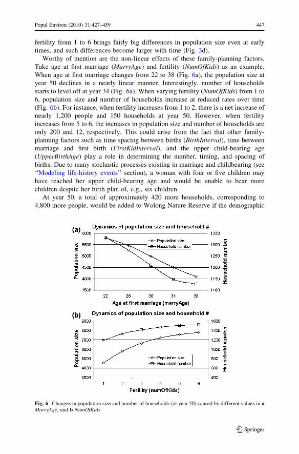
Worthy of mention are the non-linear effects of these family-planning factors.

Take age at first marriage (MarryAge) and fertility (NumOfKids) as an example.

When age at first marriage changes from 22 to 38 (Fig. 6a), the population size at

year 50 declines in a nearly linear manner. Interestingly, number of households

starts to level off at year 34 (Fig. 6a). When varying fertility (NumOfKids) from 1 to

6, population size and number of households increase at reduced rates over time

(Fig. 6b). For instance, when fertility increases from 1 to 2, there is a net increase of

nearly 1,200 people and 150 households at year 50. However, when fertility

increases from 5 to 6, the increases in population size and number of households are

only 200 and 12, respectively. This could arise from the fact that other family-

planning factors such as time spacing between births (BirthInterval), time between

marriage and first birth (FirstKidInterval), and the upper child-bearing age

(UpperBirthAge) play a role in determining the number, timing, and spacing of

births. Due to many stochastic processes existing in marriage and childbearing (see

‘‘Modeling life-history events’’ section), a woman with four or five children may

have reached her upper child-bearing age and would be unable to bear more

children despite her birth plan of, e.g., six children.

At year 50, a total of approximately 420 more households, corresponding to

4,800 more people, would be added to Wolong Nature Reserve if the demographic

Fig. 6 Changes in population size and number of households (at year 50) caused by different values in aMarryAge, and b NumOfKids

Popul Environ (2010) 31:427–459 447

123

expansion scenario replaces the baseline scenario (Fig. 7a, b). If the demographic

contraction scenario is implemented, a total of 3,300 people and 335 households

would be taken away from the baseline scenario at year 50. At year 38, the number

of households begins to decline in the demographic contraction scenario (Fig. 7b),

and the differences between the demographic expansion and contraction scenarios

become increasingly large over time.

Effects of family-planning scenarios on panda habitat

Considering the habitat changes caused by individual factors, age at first marriage

(MarryAge) and upper child-bearing age (UpperBirthAge) yield the two largest

values, i.e., 8 km2 between MarryAge = 38 and 18 (Fig. 5a) and 10 km2 between

UpperBirthAge = 30 and 55 (Fig. 5e). Fertility (NumOfKids), when taking 1 and 6,

gives a difference of 5.6 km2 in habitat at year 50 (Fig. 5d), while time spacing

between births (BirthInterval) and time between marriage and first birth (FirstKid-Interval) lead to the smallest difference in panda habitat, both at 2.5–2.6 km2

(Fig. 5b, c). In terms of the timing when a relatively large difference in habitat (e.g.,

3 km2) takes place, age of first marriage, upper child-bearing age, and fertility make

this happen between years 10 and 11, years 24 and 25, and years 40 and 41,

respectively. In terms of total differences in panda habitat caused by the two

comprehensive scenarios, there is a difference of around 20 km2 at year 50

(Fig. 7c).

The habitat becomes slightly more fragmented over time, in parallel with a

slightly higher clumpedness for the overall landscape, suggesting that non-habitat

becomes more clumped. The number of patches does not change much among

Fig. 7 a Population dynamics, b household dynamics, and c panda habitat dynamics in demographiccontraction, baseline, and demographic expansion scenarios

448 Popul Environ (2010) 31:427–459

123

different scenarios, but habitat patch size decreases from year 0 (393.17 ha) to year

50 in all three scenarios (around 313–322 ha; Table 2). Habitat connectivity

measured by cohesion does not change much (all around 96). The Shannon evenness

index has a moderate decrease from 0.90 at year 0 to around 0.85 at year 50, and

again does not differ much between the three scenarios. We will discuss the possible

reason(s) and implications of such results in the next section.

Further spatial analysis focusing on local habitat changes shows that the areas

near existing human settlements (Fig. 1) are deforested with varying probabilities in

the baseline scenario (Fig. 8b). In the demographic contraction scenario, the saved

habitat has an average elevation of 2,430 m and slope of 20�, which are moderate in

the elevation and slope ranges for pandas (Table 3; see habitat definition in ‘‘Study

site’’ section). A large proportion of such saved habitat is in deciduous or coniferous

areas (Table 3). On the other hand, the demographic expansion scenario would

expose many near-settlement areas of habitat to destruction with varying

probabilities (Fig. 8d and Fig. 9c). The lost habitat areas, averaging 2,475 m in

Fig. 8 Spatial distribution of habitat a at year 0 (1996), b at year 50 in the baseline scenario, c at year 50in the demographic contraction scenario, and d at year 50 in the demographic expansion scenario. In thegradient between 0 and 1, 0 stands for completely non-habitat, and 1 completely habitat

Popul Environ (2010) 31:427–459 449

123

Table 3 Descriptive statistics of lost or saved habitat

Habitata Average Max. Min. SD Area of panda habitat under each

vegetation type (km2)

Deciduous Conifer Mixed

Lost habitat in

demographic

expansion scenario

Elevation (m) 2,475 2,991 2,062 283 1.81 1.43 0.39

Slope (degree) 22 29 5 6 Total: 3.63

Saved habitat in

demographic

contraction scenario

Elevation (m) 2,430 3,020 1,703 304 2.98 3.11 1.56

Slope (degree) 20 29 2 7 Total: 7.65

a The lost habitat is the difference of habitat between the baseline and demographic expansion scenarios

at year 50. We calculate the habitat of baseline and demographic expansion scenarios using the criteria

mentioned in ‘‘Study site’’ The habitat in each scenario is comprised of cells with probability C 0.50 (see

footnote 12) out of the 30 replicates. Similar explanations apply to the saved habitat in the demographic

contraction scenario

Fig. 9 Locations of a lost habitat at year 50 (2046, compared to year 0 or year 1996) in the baselinescenario, b saved habitat in the demographic contraction scenario, c lost habitat in the demographicexpansion scenario; b and c are compared with baseline at year 50

450 Popul Environ (2010) 31:427–459

123

elevation and 22� in slope, are located mostly in deciduous or coniferous areas

(Table 3).

Discussion

The simulation experiments presented here yield important insights into the

hypothetical demographic and environmental implications of changes in family-

planning factors in the Wolong Nature Reserve. Incorporating individual-level age

and gender information, a few intra-household processes are simulated to take place

in and modify a spatially explicit environment with various biophysical and

geographic features (e.g., amount and type of vegetation, access to fuelwood), and

changes of these features may feed back into the intra-household processes. When

all the above processes or factors are simultaneously considered in our agent-based

model, several key insights emerge. First, family-planning and other fertility-related

factors (such as fertility rate, time spacing between births, and upper child-bearing

age) yield almost immediate changes in population size (Fig. 3). In particular,

decreases in upper child-bearing age could result in substantial changes in

population dynamics over time: the population difference arising from a decrease in

upper child-bearing age from 55 to 30 is nearly equal to that arising from a decrease

of fertility from 6 to 1.

Second, all the factors considered in this paper (except time at first marriage)

exhibit important time lags in their impacts on number of households at broader

scales. The variable that mostly quickly alters projected numbers of households is

age at first marriage: A decrease from 38 to 18 could give rise to a difference of 90

households at year 5. More interestingly, this difference increases over time (e.g.,

150 households at year 10), maximizes at year 20 (around 220), then decreases from

year 20 to 40, and finally increases. This phenomenon may be largely explained by

the household lifecycle: delayed marriages directly postpone the establishment of

new households and births of babies who may establish their households in a similar

or even longer time frame (Fig. 4a). It takes more time for other variables to take

effect in reducing number of households. For instance, when fertility rate

(NumOfKids) increases by 1, the added children still remain in their parental

households until they grow up and establish their own households, which explains

the 20? years of time lag (Fig. 4d). These findings have important policy

implications, and corroborate findings and thoughts regarding temporal lags

inherent in population–environment linkages (e.g., Carr et al. 2006a). As shown

earlier, if the goal is more focused on curbing unsustainable increases in population

size, then reducing fertility rate or upper child-bearing age should be more effective,

particularly when we look at the timing of such changes (Fig. 3d, e). On the other

hand, if reducing number of households as soon as possible is of more concern, a

focus on promoting an older age at first marriage (MarryAge) might be more

effective (Fig. 4a), which is the ‘‘later’’ part of the Wan-Xi-Shao policy.

Third, we discuss the effects of family-planning factors on panda habitat. Here,

we simply present our simulation results regarding how population size, number of

households, and panda habitat may respond to changes in those family-planning or

Popul Environ (2010) 31:427–459 451

123

fertility-related factors. These simulations do not represent our own attitudes or

preferences of family-planning or fertility-related factors. In terms of ultimate

influences on panda habitat, increasing the upper age to bear children (UpperBir-thAge), through sterilization at earlier ages for instance, makes the biggest

difference (approximately 10 km2; Fig. 5e) in the long run. A reduced upper

childbearing age (UpperBirthAge) from 50 to 30 can bring down population size

from approximately 5,785 to 3,400 people and number of households from 1,331

to 1,087 at year 50. Changes in other variables do not reduce population size

(Fig. 3a–d) and number of households (Fig. 4a–d) at such magnitudes. In terms of the

earliest time to cause a larger habitat difference, changes in age at first marriage

(MarryAge) make the biggest difference. By postponing this age, young people

remain at their parental homes longer, and the growth in number of households

substantially slows, which can be seen from the bottom curve (MarryAge = 38) in

Fig. 4a. The change of potential panda habitat depends more on number of

households than on population size, which is consistent with what has been found at

the global scale (Liu et al. 2003a). This may arise from the way fuelwood is

consumed. A large proportion of fuelwood is used for heating in winter, which

changes little when a new person is added to or removed from the existing household.

In consideration of cooking, the extra fuelwood caused by adding one person or the

fuelwood saved by removing one person would be small (An et al. 2001).

Last, the methods and findings in this study are important for panda habitat

conservation. As shown earlier, a decision of postponing marriages (an increase in

MarryAge) or stopping childbearing at earlier ages (a decrease in UpperBirthAge)

might result in saving panda habitat in the long run (Fig. 5a, e). However, if the goal

is to save habitat as early as possible, then an increase in upper childbearing age

might be more effective than a decrease in fertility rate. A reduction in fertility rate

(NumOfKids) does not save habitat as much as the above two options in the short

run (compare d with a and e in Fig. 5) and may be subject to more social resistance.

However, a reduction in fertility rate might still be effective over a longer term (e.g.,

over 100 years), which goes beyond our simulation time frame.

The spatial habitat patterns (Table 2) do not vary much over different family-

planning and fertility-related scenarios at early times, but such small changes may

be cumulative over a longer time period (e.g., 100 years). Second, even these

numbers can show us some useful information. For instance, the demographic

contraction scenario gives an increase of 9 ha in patch size compared with the

baseline scenario. This increasing trend is meaningful for panda conservation in the

long run (e.g., [50 years), especially when we consider the giant panda’s home

range of 200? ha per animal (Schaller et al. 1985). Patches smaller than 200 ha and

with poor connectivity with other habitat patches are not likely used by pandas.

Fortunately, most of the habitat patches are still well connected in light of the high

cohesion index values (96 out of 100; Table 2). Last, the overall landscape indices

alone do not reveal where habitat is saved or lost or the characteristics of such

habitat, which may be equally (if not more) important for pandas.

Our analyses disclose not only the spatial distribution of panda habitat in the

baseline (Fig. 8b), demographic contraction (Fig. 8c), and demographic expansion

(Fig. 8d) scenarios, but also the locations and characteristics of net habitat lost or

452 Popul Environ (2010) 31:427–459

123

saved in these scenarios. We have shown that the lost or saved habitat is of moderate

elevation and slope and in areas of deciduous or coniferous forests. This may play a

very important role in affecting panda activities because areas with such

characteristics are more preferred by pandas (see ‘‘Study site’’ section for habitat

definition). Such information would be more valuable in combination with other

ecological or biological data. For instance, if the lost areas break existing corridors

connecting separate habitat patches, panda metapopulations may suffer from lack of

dispersal, inadequacy of genetic flow, and high likelihood of local extinction

(Drechsler et al. 2003).

Conclusions

Our bottom-up approach simulates micro-level (intra-household) population

processes and the corresponding environmental responses in a spatially explicit

manner, incorporating many individual- or household-level decisions, environmen-

tal heterogeneity, and feedbacks. This approach thus has the potential to integrate

multidisciplinary data and continuous processes operating across varying commen-

surate spatial and temporal scales (An et al. 2005). This potential helps to address

many issues inherent in many population–environment studies, such as choosing the

appropriate spatial/temporal scales or handling ‘‘spatial and temporal discontinu-

ities’’ in data or analysis (Carr et al. 2006a). As a result, we have observed what

researchers in complexity theory call ‘‘emergence’’ (see ‘‘Background’’ section).

For instance, the non-linear relationships between changes in number of households

and the increases in age at first marriage are not easily detected (Fig. 4a) unless we

take into account the many relevant individual-level data or decisions as discussed

earlier. Another example of observed emergence is how population size and number

of households respond differently to changes in age at first marriage (Fig. 6a):

population size has a near-linear decline as the age goes up, while number of

households decreases at a reduced rate when the age is greater than 34 (earlier we

have briefly discussed possible reasons). This bottom-up approach may also explain

the different responses of number of households and population size when fertility

(NumOfKids) changes (Fig. 6b).

However, like many other models, our model is a simplified representation of the

real-world patterns and processes under investigation, although it has been

calibrated using empirical data and has passed a series of model testing procedures

(An et al. 2005). Thus, we use the model more as a laboratory of the coupled

human–nature system to answer what-if questions than as a tool to accurately

predict population, households, and habitat. More experiments could be conducted

using such a laboratory, answering questions that were not addressed in this study,

such as ‘‘How would population size, number of households, and panda habitat

dynamics respond to varying initial population age structure caused by different

types of migrations?’’ Also worthy of mention is the model’s capacity to link

various types of data/findings and mimic different processes over time. For

example, although we treat fertility as an exogenous variable for the goals of this

paper, we can endogenize fertility and link it to other variables such as farm size and

Popul Environ (2010) 31:427–459 453

123

tenure (Coomes et al. 2001), distance to market (Carr et al. 2006b), and resource

dependency (Dasgupta 2000) in other instances.

We hope that all such efforts could introduce new perspectives into studies of

human demography, especially household and family demography that was

considered ‘‘a recent and relatively underdeveloped branch of population studies’’

(Bongaarts 2001). These new perspectives, the agent-based bottom-up approach in

particular, may help to form more scientifically grounded policy and yield a more

sustainable future for both humans and the natural environment.

Acknowledgments We are indebted to financial support from the National Science Foundation

(Dynamics of Coupled Natural and Human Systems, Partnership for International Research and

Education), the National Institute of Child Health and Human Development (R01 HD39789), the National

Aeronautics and Space Administration (Land Use/Land Cover Change program and Terrestrial Ecology

and Biodiversity program), the Guggenheim Foundation, Michigan State University, and San Diego State

University. We also thank Dean Daniels, Guangming He, Marc Linderman, Zhiyun Ouyang, Andres

Vina, Hemin Zhang, and Shiqiang Zhou for their assistance in data acquisition and processing. We are

grateful to Joanna Broderick, Lori Hunter, and anonymous reviewers for their constructive comments on

earlier versions of this paper. The data collection and analyses (including computer experiments)

conducted in this article comply with the current laws of China.

References

An, L., Linderman, M. A., Shortridge, A., Qi, J., & Liu, J. (2005). Exploring complexity in a human-

environment system: An agent-based spatial model for multidisciplinary and multi-scale integration.

Annals of Association of American Geographers, 95(1), 54–79.

An, L., Liu, J., Ouyang, Z., Linderman, M. A., Zhou, S., & Zhang, H. (2001). Simulating demographic

and socioeconomic processes on household level and implications on giant panda habitat.

Ecological Modeling, 140, 31–49.

An, L., Lupi, F., Liu, J., Linderman, M. A., & Huang, J. (2002). Modeling the switch from fuelwood to

electricity: implications for giant panda habitat conservation. Ecological Economics, 42(3), 445–

457.

An, L., Mertig, A. G., & Liu, J. (2003). Adolescents’ leaving parental home: Psychosocial correlates and

implications for biodiversity conservation. Population and Environment: A Journal of Interdisci-plinary Studies, 24(5), 415–444.

Axinn, W., Ghimire, D. (2007). Social organization, population, and land use. PSC Research Report No.

07-617 (http://www.psc.isr.umich.edu/pubs/pdf/rr07-617.pdf). February 2007.

Barabasi, A. L., Jeong, H., & Albert, R. (1999). The diameter of the World Wide Web. Nature, 401, 130–

131.

Bearer, S. L., Linderman, M., Huang, J., An, L., He, G., & Liu, J. (2008). Effects of fuelwood collection

and timber harvesting on giant panda habitat use. Biological Conservation, 141(2), 385–393.

Billari, F. C., & Prskawetz, A. (Eds.). (2003). Agent-based computational demography: Using simulationto improve our understanding of demographic behaviour (contributions to economics). Heidelberg:

Physica-Verlag.

Bilsborrow, R., & Dleargy, P. (1991). Land use, migration, and natural resources deterioration: The

experience of Guatemala and the Sudan. In K. Davis & M. Bernstam (Eds.), Resources,environment, and population. Oxford: Oxford University Press.

Birdsall, N. (1988). Economic approaches to population growth. In H. Chenery & T. N. Srinivasan (Eds.),

Handbook of development economics. Amsterdam: North Holland.

Bongaarts, J. (1978). Framework for analyzing proximate determinants of fertility. Population andDevelopment Review, 4(1), 105–132.

Bongaarts, J. (1996). Population pressure and the food supply system in the developing world. Populationand Development Review, 22(3), 483–503.

454 Popul Environ (2010) 31:427–459

123

Bongaarts, J. (2001). Household size and composition in the developing world in the 1990s. PopulationStudies-A Journal of Demography, 55, 263–279.

Boserup, E. (1965). The conditions of agricultural growth. London: Earthscan.

Brown, A. D. (2003). Feed or feedback: Agriculture, population dynamics and the state of the planet.Tuross Head, Australia: International Books.

Bryant, L., Carver, L., Butler, C. D., & Anage, A. (2009). Climate change and family planning: Least-

developed countries define the agenda. Bulletin of the World Health Organization, 87, 852–857.

Carr, D. L. (2004). Proximate population factors and deforestation in tropical agricultural frontiers.

Population and Environment, 25(6), 585–612.

Carr, D. L., Pan, W. K., & Bilsborrow, R. E. (2006a). Declining fertility on the frontier: The Ecuadorian

Amazon. Population and Environment, 28(1), 17–39.

Carr, D. L., Suter, L., & Barbieri, A. (2006b). Population dynamics and tropical deforestation: State of the

debate and conceptual challenges. Population and Environment, 27(1), 89–113.

Castella, J., Trung, T. N., & Boissau, S. (2005). Participatory simulation of land-use changes in the

northern mountains of Vietnam: The combined use of an agent-based model, a role-playing game,

and a geographic information system. Ecology and Society, 10(1), 27.

Cho, I. (2005). Introduction to learning and bounded rationality. Journal of Economic Theory, 124, 127–

128.

Clarke, J. G., Hebert, M. R., Rosengard, C., Rose, J. S., DaSilva, K. M., & Stein, M. D. (2006).

Reproductive health care and family planning needs in incarcerated women. American Journal ofPublic Health, 96(5), 834–839.

Clay, D. C., & Johnson, N. E. (1992). Size of farm or size of family: Which comes first? PopulationStudies, 46, 491–505.

Cohen, J. E. (1995). How many people can the earth support?. New York: W.W. Norton & Company.

Cohen, J. E. (2003). Human population: The next half century. Science, 302(5648), 1172–1175.

Coomes, O.T., Grimard, F., & Diaz, V (2001). Peasant farm size and family size: a causality analysisfrom the Peruvian Amazon. Working Paper, Department of Geography, McGill University,

Montreal.

Dasgupta, P. (2000). Population and resources: An exploration of reproductive and environmental

externalities. Population and Development Review, 26(2000), 643–689.

de Sherbinin, A., Carr, D., Cassels, S., & Jiang, L. (2007). Population and environment. Annual Review ofEnvironment and Resources, 32, 345–373.

de Sherbinin, A., VanWey, L. K., McSweeney, K., Aggarwal, R., Barbieri, A., Henry, S., et al. (2008).

Rural household micro-demographics, livelihoods and the environment. Global EnvironmentalChange, 18, 38–53.

Deadman, P., Robinson, D., Moran, E., & Brondizio, E. (2004). Colonist household decisionmaking and

land-use change in the Amazon Rainforests: An agent-based simulation. Environment and PlanningB, 31, 693–709. 2007.

Demographic and Health Surveys (2009). http://www.measuredhs.com/topics/fp/start.cfm (last accessed

Nov 3, 2009).

Dietz, T., & Rosa, E. . A. (1997). Effects of population and affluence on CO2 emissions. Proceedings ofthe Natural Academy of Sciences, 94, 175–179.

Drechsler, M., Frank, K., Hanski, I., O’Hara, R. B., & Wissel, C. (2003). Ranking metapopulation

extinction risk: From patterns in data to conservation management decisions. EcologicalApplications, 13, 990–998.

Ehrlich, P. R. (1968). The population bomb. New York: Ballantine Books.

Ehrlich, P., & Ehrlich, A. (2006). Enough already. New Scientist, 191(2571), 46–50.

Ehrlich, P. R., & Holdren, J. P. (1972). A bulletin dialogue on the ‘‘closing circle’’: Critique: One-

dimensional ecology. Bulletin of the Atomic Scientists, 28(5), 16–27.

Entwisle, B. (2001). Population and land use in Nang Rong, Thailand. Paper presented at the Annual

Meeting of the Population Association of America, March 29–31, Washington D.C.

Entwisle, B. (2007). Putting people into place. Demography, 44(4), 687–703.

Environmental Systems Research Institute (ESRI). (2007). ArcGIS version 8.0–9.2. California: Redlands.

Eryilmaz, G. (2006). The evaluation of family planning services given in erzurum mother-child health

and family planning center in Eastern Turkey. The European Journal of Contraception andReproductive Health, 11(2), 146–150.

Evans, T. P., & Kelly, H. (2004). Multi-scale analysis of a household level agent-based model of land

cover change. Journal of Environmental Management, 72, 57–72.

Popul Environ (2010) 31:427–459 455

123

Feeney, G., & Feng, W. (1993). Parity progression and birth intervals in China—the influence of policy in

hastening fertility decline. Population and Development Review, 19(1), 61–101.

Feng, G., & Hao, L. (1992). Summary of 28 regional birth planning regulations in China. PopulationResearch (Renkou Yanjiu; in Chinese), 4, 28–33.

Foster, D. G., Biggs, M. A., Amaral, G., Brindis, C., Navarro, S., Bradsberry, M., et al. (2006). Estimates

of pregnancies averted through California’s family planning waiver program in 2002. Perspectiveson Sexual and Reproductive Health, 38(3), 126–131.

Freedman, R. (1997). Do family planning programs affect fertility preferences? A literature review.

Studies in Family Planning, 28(1), 1–13.

Fricke, T. E. (1986). Himalayan households: Tamang demography and domestic processes. Ann Arbor:

UMI Research Press.

Gaffikin, L. (2007). Family planning: building blocks to a better environment and better world.

Population and Environment, 28(4–5), 283–288.

Ghimire, D. J., & Hoelter, L. F. (2007). Land use and first birth timing in an agricultural setting.

Population and Environment, 28(6), 289–320.

Hempel, M. (1997). Why population matters. Population and Environment, 18, 561–563.

Hobcraft, J., Menken, J., & Preston, S. (1982). Age, period, and cohort effects in demography: A review.

Population Index, 48(1), 4–43.

Hong, R., Montana, L., & Mishra, V. (2006). Family planning services quality as a determinant of use of

IUD in Egypt. BMC Health Services Research, 6: 79. Available online at http://www.biomedcentral.

com/1472-6963/6/79.

Hunter, L. (2001). The environmental implications of population dynamics. Population Matters Series.

Santa Monica, California: RAND.

Hunter, L. M., Twine, W., & Patterson, L. (2007). ‘‘Locusts are now our beef’’: Adult mortality and

household dietary use of local environmental resources in rural South Africa. Scandinavian Journalof Public Health, 35(Suppl. 69), 165–174.

Hussain, A. (2002). Demographic transition in China and its implication. World Development, 30(10),

1823–1834.

Hutchinson, P., & Wheeler, J. (2006). Advanced methods for evaluating the impact of family planning

communication programs: Evidence from Tanzania and Nepal. Studies in Family Planning, 37(3),

169–186.

Jones, G. W. (2007). Delayed marriage and very low fertility in Pacific Asia. Population andDevelopment Review, 33, 453–478.

Keyfitz, N. (1976). Mathematical demography: A bibliographical essay. Population Index, 42(1), 9–38.

Keyfitz, N. (1993). Thirty years of demography and demography. Demography, 30(4), 533–549.

Kohler, H.P., & Ortega, J.A. (2002). Tempo-adjusted period parity progression measures, fertility

postponement and completed cohort fertility. Demographic Research, 6, 91–144. Online at

www.demographic-research.org/Volumes/Vol6/6/.

Lee, J., & Feng, W. (1999). Malthusian models and Chinese realities: The Chinese demographic system

1700–2000. Population and Development Review, 25, 33–65.

Liang, Z., & Ma, Z. (2004). China’s floating population: New evidence from the 2000 census. Populationand Development Review, 30(3), 467–488.

Linderman, M., Liu, J., Qi, J., Ouyang, Z., An, L., Yang, J., et al. (2004). Using artificial neural networks

to map the spatial distribution of understory bamboo from remote sensing data. InternationalJournal of Remote Sensing, 25(6), 1685–1700.

Liu, Z. Q. (2005). Institution and inequality: The hukou system in China. Journal of ComparativeEconomics, 33(1), 133–157.

Liu, J., Daily, G. C., Ehrlich, P. R., & Luck, G. W. (2003a). Effects of household dynamics on resource

consumption and biodiversity. Nature, 421, 530–533.

Liu, J., Dietz, T., Carpenter, S., Alberti, M., Folke, C., Moran, E., et al. (2007a). Complexity of coupled

human and natural systems. Science, 317, 1513–1516.

Liu, J., Dietz, T., Carpenter, S., Folke, C., Alberti, M., Redman, C., et al. (2007b). Coupled human and

natural systems. Ambio, 36, 639–649.

Liu, J., Linderman, M., Ouyang, Z., An, L., Yang, J., & Zhang, H. (2001). Ecological degradation in

protected areas. Science, 292, 98–101.

Liu, J., Ouyang, Z., Linderman, M., An, L., Bearer, S., & He, G. (2003b). A new paradigm for panda

research and conservation: Integrating ecology with human demography, behavior, and

456 Popul Environ (2010) 31:427–459

123

socioeconomics. In D. G. Lindburg & K. Baragona (Eds.), Giant Panda: Conservation priorities forthe 21st century. Berkeley: University of California Press.

Liu, J., Ouyang, Z., Tan, Y., Yang, J., & Zhang, H. (1999a). Changes in human population structure:

Implications for biodiversity. Population and Environment: A Journal of Interdisciplinary Studies,21, 46–58.

Liu, J., Ouyang, Z., Taylor, W. W., Groop, R., & Zhang, H. (1999b). A framework for evaluating the

effects of human factors on wildlife habitat: The case of giant pandas. Conservation Biology, 13,

1360–1370.

Liu, T., & Zhang, X. (2009). Ratio of males to females in China. British Medical Journal, 338, b483.

Lustick, I. S. (2000). Agent-based modelling of collective identity: Testing constructivist theory. Journalof Artificial Societies and Social Simulations, 3(1), 1–21.

Malthus, T. R. (1798). An Essay on the Principle of Population. Ann Arbor: University of Michigan

Press. [1959].

Manson, S. M. (2001). Simplifying complexity: A review of complexity theory. Geoforum, 32(2001),

405–414.

Marcoux, A. (1999). Population and Environment Change: from Linkages to Policy Issues. (http://www.fao.org/

sd/wpdirect/WPre0089.htm).

McCracken, S. D., Siqueira, A. D., Moran, E., & Brondızio, E. S. (2002). Land use patterns on an

agricultural frontier in Brazil: Insights and examples from a demographic perspective. In C. H.

Wood & R. Porro (Eds.), Deforestation and land use in the Amazon (pp. 162–192). Gainesville, FL:

University Press of Florida.

McGarigal, K., Cushman, S.A., Neel, M.C., & Ene, E. (2002). FRAGSTATS: Spatial pattern analysis

program for categorical maps. Computer software program produced by the authors at the

University of Massachusetts, Amherst. Available at the following web site: www.umass.edu/

landeco/research/fragstats/fragstats.html.

McSweeney, K. (2004). Forest product sale as natural insurance: The effects of household charateristics

and the nature of shock in eastern Honduras. Society and Natural Resources, 17(1), 39–56.

McSweeney, K. (2005). Natural insurance, forest access, and compounded misfortune: Forest resources in

smallholder coping strategies before and after Hurricane Mitch, eastern Honduras. WorldDevelopment, 33(9), 1453–1471.

Meadows, D. H., Meadows, D. L., Randers, J., & Behrens III, W. W. (1972). The limits to growth. New

York: Universe Books.

Messina, J. P., & Walsh, S. J. (2005). Dynamic spatial simulation modeling of the population—

environment matrix in the Ecuadorian Amazon. Environment and Planning B: Planning and Design,32(6), 835–856.

Moran, E. F., Brondizo, E. S., & VanWey, L. K. (2005). Population and environment in Amazonia:

Landscape and household dynamics. In National Research Council’s Population, Land Use, andEnvironment. Washington D.C.: National Academics Press.

Moran, E. F., Siqueira, A., & Brondizio, E. S. (2002). Household demographic structure and its

relationship to deforestation in the Amazon Basin. In J. Fox, R. Rindfuss, S. Walsh, & V. Mishra

(Eds.), People and the environment: Approaches to linking household and community surveys toremote sensing and GIS (pp. 61–89). New York, NY: Kluwer.

Murphy, L. L. (2001). Colonist farm income, off-farm work, cattle, and differentiation in Ecuador’s

northern Amazon. Human Organization, 60(1), 67–79.

Myers, N., Mittermeier, R. A., Mittermeier, C. G., da Fonseca, G. A. B., & Kent, J. (2000). Biodiversity

hotspots for conservation priorities. Nature, 403, 853–858.

National Population and Family Planning Commission of China (NPFPC). (2008). Regulation on

Missions, Organizational Structure and Composition of NPFPC. http://www.npfpc.gov.cn/en/

about/detail.aspx?articleid=090427111022687682 (last accessed on March 02 2010).

Pebley, A. R. (1998). Demography and the environment. Demography, 35(4), 377–389.

Population Council (1998). Clinic-based family planning and reproductive health services in Africa:

Findings from situation analysis studies. In Miller, K., Miller, R., Askew, I., Horn, M.C., Ndhlovu,

L. (Eds.). Available online at http://pdf.dec.org/pdf_docs/Pnace366.pdf.

Population Reference Bureau (PRB) (2009). http://www.prb.org/Publications/ Datasheets/2009/

2009wpds.aspx (last accessed Nov 3, 2009).

Preston, S. H. (1993). The contours of demography: Estimates and projections. Demography, 30(4),

593–606.

Popul Environ (2010) 31:427–459 457

123

Rindfuss, R. (1991). The young adult years: Diversity, structural change, and fertility. Demography, 28,

493–512.

Robinson, D. T., & Brown, D. G. (2009). Evaluating the effects of land-use development policies on

ex-urban forest cover: An integrated agent-based GIS approach. International Journal ofGeographical Information Science, 23(9), 1211–1232.

Ross, J. A., & Issacs, S. L. (1988). Costs, payments, and incentives in family planning programs: A

review for developing countries. Studies in Family Planning, 19(5), 270–283.

Sable, M. R., Campbell, J. D., Schwarz, L. R., Brandt, J., & Dannerbeck, A. (2006). Male Hispanic

immigrants talk about family planning. Journal of Health Care for the Poor and Underserved, 17,

386–399.

Schaller, G. B., Hu, J., Pan, W., & Zhu, J. (1985). The giant pandas of Wolong. Chicago: The University

of Chicago Press.

Simon, J. (1990). Population matters: People, resources, environment, and immigration. New Brunswick,

NJ: Transaction.

Sinding, S. W. (2000). The great population debates: How relevant are they for the 21st century?

American Journal of Public Health, 90, 1841–1845.

Spiedel, J., Weiss, D., Ethelston, S., & Gilbert, S. (2007). Family planning and reproductive health: The

link to environmental preservation. Population and Environment, 28(4–5), 247–258.

Steiner, M. J., Trussell, J., Mehta, N., Condon, S., Subramanniam, S., & Bourne, D. (2006).

Communicating contraceptive effectiveness: A randomized controlled trial to inform a world health

organization family planning handbook. American Journal of Obstetrics and Gynecology, 195, 85–

91.

Stokes, C. S., & Schutjer, W. A. (1984). Access to land and fertility in developing countries. In W. A.

Schutijer & C. S. Stokes (Eds.), Rural development and human fertility. New York: McMillan.

Strauss, J., & Thomas, D. (1995). Human resources: Empirical modeling of household and family

decisions. In J. Behrman & T. N. Srinivasan (Eds.), Handbook of development economics (Vol.

iii(A)). Amesterdam: North Holland.

Sutherland, E., Carr, D.L., Curtis, S. (2004). Fertility and the environment in a natural resourcedependent economy: Evidence from Peten, Guatemala. California Center for Population Research.

The Population of the Central American Isthmus in 2003. Conference Papers. Paper ccpr-cp-010-05.

http://repositories.cdlib.org/ccpr/olcp/ccpr-cp-010-05.

Turner, M. G., Gardner, R. H., & O’Neill, R. V. (2001). Landscape ecology in theory and practice:Pattern and process. New York: Springer.

U.S. Census Bureau (2009). U.S. and World Population Clocks—POPClocks. Online available at

http://www.census.gov/ipc/www/popclockworld.html.

United Nations Population Division (UNPD) (2009). http://www.un.org/esa/population/unpop.htm.

U.S. National Academy of Sciences. (1963). The growth of world population. Washington, DC: National

Academy of Sciences.

VanWey, L. K., D’Antona, A. O., & Brondizio, E. S. (2007). Household demographic change and land

use/land cover change in the Brazilian Amazon. Population and Environment, 28(3), 163–185.

Vitousek, P. M. (1994). Beyond global warming: Ecology and global change. Ecology, 75(7), 1861–1876.

Walsh, S., Rindfuss, R., Prasartkul, P., Entwisle, B., & Chamratrithirong, A. (2005). Population change

and landscape dynamics: The Nana Rong, Thailand studies. In B. Entwisle & P. C. Stern (Eds.),

Population, land use, and environment. Washington D.C.: National Academy Press.

Wenchuan County. (2006). Statistical year book of Wenchuan County, 2006 (in Chinese). China: Sichuan

Province.

Wilk, R. (1990). Household ecology: decision making and resource flows. In E. Moran (Ed.), Theecosystem approach in anthropology: From concept to practice (pp. 323–356). Michigan:

University of Michigan Press.

Wolong Nature Reserve (1997). 1996 Agricultural Census, Wolong (unpublished, in Chinese).

Wolong Nature Reserve (2000). 2000 Nationwide Population Census (Wolong) Form (unpublished, in

Chinese).

Wong, J. (2001). China’s sharply declining fertility: Implications for its population policy. Issues andStudies, 37(3), 68–86.

Wood, C. H., & Skole, D. (1998). Linking satellite, census, and survey data to study deforestation in the

Brazilian Amazon. In D. Liverman, E. F. Moran, R. R. Rindfuss, & P. C. Stern (Eds.), People andpixels: Linking remote sensing and social science (pp. 70–93). Washington, D.C.: National

Academy Press.

458 Popul Environ (2010) 31:427–459

123

World Health Organization (WHO) (2009). http://www.who.int/topics/family_planning/en/.

World Wildlife Fund (WWF) (2010). http://www.panda.org/what_we_do/endangered_species/giant_

panda/solutions/pandasuccess/.

Yang, Y., & Li, C. (Eds.). (1992). Sichuan forests. Beijing, China: Yunnan, China Forestry Press.

Yin, H. W. (2005). A living report of giant pandas in Wolong. New Western, 6, 37–39.

Yu, E., & Liu, J. (2007). Environmental impacts of divorce. PNAS 104 (51), 20629–20634.

http://www.csis.msu.edu/Publications/PNAS_divorce_environment.pdf.

Zhang, H., Li, D., Wei, R., Tang, C., & Tu, J. (1997). Advances in conservation and studies on

reproductivity of giant pandas in Wolong. Sichuan Journal of Zoology, 16, 31–33.

Popul Environ (2010) 31:427–459 459

123