Long-run trends in earningsand employment

in Hungary, 1972–1996

ÁRPÁD ÁBRAHÁM and GÁBOR KÉZDI

Budapest Working Papers on the Labour Market

BWP. 2000/2

February 2000

Budapest Working Papers No.2000/2Labour Research Department, Institute of Economics, Hungarian Academy of SciencesDepartment of Human Resources, Budapest University of Economics

Long-run trends in earnings and employment in Hungary,1972–1996

Authors: Árpád ÁBRAHÁM, Universitat Pompeu Fabra, Barcelona; and LabourResearch Department Institute of Economics Hungarian Academy ofSciences. E-mail: abraham@upf.es and abraham@econ.core huGábor KÉZDI, University of Michigan, Ann Arbor; and Labour ResearchDepartment Institute of Economics Hungarian Academy of Sciences.E-mail: kezdi@umich.edu and kezdi@econ.core.hu

Published by the Institute of Economics, Hungarian Academy of Sciences. Budapest, 2000.With financial support from the Foundation for Job Creation

and the Foundation Budapest Bank for Budapest

LONG-RUN TRENDS IN EARNINGSAND EMPLOYMENT

IN HUNGARY, 1972-19961

ÁRPÁD ÁBRAHÁM and GÁBOR KÉZDI

Transition from socialist to capitalist economy led to enormouschanges in earnings and employment. In our study a long-horizondescriptive analysis is presented about the major trends, including thelast fifteen years of socialism. Education, gender, calendar time, ageand vintage effects are separately analyzed. Aggregate (quasi-) panelanalysis is used to assess the role of labor demand and labor supply,concluding that exogenous supply factors explained most of whathappened before the transition, while the transition itself wasdominated by large labor demand shocks. These demand shocks are inlarge part structural, as opposed to cyclical, and are highly correlatedwith vintage, gender and education. The main results are summarizedin a list of stylized facts.

1. INTRODUCTION

The motivation of this paper is to provide a comprehensive study of themajor trends on the labor market in the last two decades of socialism andthe transition (for the period 1972–1996). There are excellent studies aboutwages and earnings as well as employment and unemployment. Most ofthem address some specific problems in addition to descriptive analysis. 1 Comments of the participants of the Budapest Workshop on the Labor Market (1998)were very helpful. We also thank Zsombor Gergely for his help. Financial support fromthe OTKA grant of the Hungarian Academy of Sciences and the Phare ACE program ofthe European Union is acknowledged. All errors are ours. Contact: abraham@upf.es orkezdi@umich.edu.

Kertesi–Köllô (1997, 1998, 1999a, 1999b), are such papers, just tomention a few. Our study is new in three respects. We examine a widertime-horizon, we follow trends in wages and employment in a unifiedframework, and partly for these reasons, we follow a longitudinal approachas opposed to the mostly cross-sectional ones mentioned above. We focuson providing a general picture, with cohort effects and longitudinalanalysis.

This is an empirical study, based on a number of different data sources.Our data has quasi-panel structure: time-series of consecutive cross-sections in gender-schooling-cohort cells. This allows us to decomposeand analyze the wage - labor supply relationship along the majordemographic dimensions. The advantages of this approach are comingfrom the fact that we are following groups of people: these attributes don'tchange over time and transitory effects are averaged out. Thedisadvantages are also coming from the grouping: this is not a real panel,hence variability is reduced and we have measurement error in variablesbecause they are sample estimates. Naturally, the enormous compression ofthe information makes it impossible to examine many finer details. On theother hand, it enables us to concentrate on the general trends and theirinteractions.

The main objective is to establish stylized facts that are relevant foreconomic policy and can be subject of further studies. Even among themostly descriptive results, some of our findings may be controversial andquestionable, or our interpretation may be incorrect. Our goal is to initiatediscussion about these facts. Comparison with results from other transitioneconomies would be welcome.

The structure of the paper is the following: in the second section wedescribe the data we used, then we proceed with a descriptive analysis inthe third section. The fourth section provides the decomposition of thetrend in wage inequality into cohort and year effects and establishes age-earnings profiles. The econometric analysis is completed by a panel studyof the changes in wages and labor supply. At the end, we summarize whatwe think the most important results in a list of stylized facts and conclude.

2. THE DATA

We used four different kinds of data sources to construct our "quasi-panel"database. (1) The Hungarian Central Statistical Office (CSO) conducted 4major surveys in the 1970s and the 1980s that provide us with detailed andvalid employment and earnings data (the latter collected from both therespondent and the employer). These were the Income Surveys (CSO IS-s)of 1973, 1978, 1983, and 1988, and the information in them was related tothe preceding year (1972, 1977, 1982, and 1987). (2) The 1990 Censusprovides us with participation, unemployment and self-employment datafor the year 1989. (3) From 1992 on, the CSO has been conducting a LaborForce Survey (CSO LFS) on a quarterly basis. Among other things, thissurvey contains ILO-standard measures of participation andunemployment, but it does not contain any information about earnings. (4)The fourth data source we use are the Wage Surveys of the National LaborCenter (NLC WS) that provide us with the earnings data from the mid-1980s on, collected from the employers. For more detailed description ofthe data see the Data Appendix.

Our analysis focuses on a limited number of variables. Besides gender,date of birth and schooling, we use labor force participation, employment(and unemployment), wage/salary and full-time wage/salary employment,and monthly earnings, including wages and other work-related income. Inwhat follows, we use the term wages and earnings in an interchangeableway, although we always mean monthly net earnings. The definition andmeasurement of these variables are explained in the Data Appendix. Oneimportant feature of the earnings data is that they are net (as opposed togross) measures. Personal income tax was introduced in 1988 in Hungary,in a way that the 1988 earnings were "grossed up" such that they matcheddisposable earnings of the previous years. In a long-run comparison,therefore, one has to use the net variable. In addition, since we focus moreon the supply side of the labor market, it is natural to consider earningsthat people receive, as opposed to total costs of labor. The net figures are,

however, estimates, which we think are biased downward (although wehave no evidence proving this, see the Data Appendix, again).

The multi-source nature of our data raises questions aboutcompatibility. Participation and employment are measured in the same wayin the three different surveys, in general. The most important exception isunemployment, and therefore, labor force participation. Unemployment ismeasured by the ILO standards in the surveys we use from 1992 on, but itis based on (self-reported) registration in 1989. Some less importantfigures are interpolated from other surveys, see the Data Appendix. Thecompatibility of the earnings data is more of an issue. We have 2 types ofsources, one (CSO IS) representing the total population, and one (NCLWS) representing those working in not too small firms (20 or moreemployees). The 1987 CSO IS and the 1986 NCL WS offer somepossibility to judge whether it is valid to compare earnings from the twosources. As Table 5 and Figures 8-12 in the next section show, theestimates of mean and group-mean earnings seem to line up reasonablywell. Table 6 and Figures 13-14 suggest that there is a significantdifference in the dispersion of wages between the two surveys, but thisdifference may be part of an existing trend. We conclude that even if thereare significant discrepancies in the two sources, our estimates are notbiased much from them, possibly because of the aggregation.

The basis of our analysis is a time-series of independent cross-sections,that is a panel, or as we call, quasi-panels database. For particular groupsof people, we estimated participation, employment and other "quantity"variables, and the mean and variance of earnings from the original datasets. These groups were defined by year of birth (in 5-year-wide intervals),gender and educational attainment (in 3 categories: 0-11 classes, secondaryschool and college or more educated). Our data set is a collection of theseestimates, connected for each group through the years. We have 49-51observations ("cells") in a particular year. Note that the characteristics thatdefine a group don't change for an individual, therefore the quasi-panelallows us to follow groups of the same people. The advantage of thisapproach, we hope, is apparent in the two last sections of this paper.

Similar aggregate quasi-panels are used in the literature, although some ofthem connect people of the same age group instead of the same years ofbirth. See, for example, Deaton (1997, Chapter 2), or Katz and Murphy(1992). Note, that these data sets are technically panels, we use the quasi-term only to distinguish them from individual or household-panels thatfollow individuals themselves.

The large samples enable us to get quite precise estimates for the cells.We estimated the standard errors of the proportion estimates (e.g. laborforce participation rate), and the mean earnings by bootstrap, except whenthe bootstrapping results indicated smaller sampling error than the simplerandom sampling estimates.2 In the CSO Income Surveys, and the CSOLabor Force Surveys the former ones always exceeded the latter ones,while in the NLC Wage Surveys the bootstrap estimates were almostalways smaller, partly because of the enormous sample sizes, and partlyperhaps because of efficient stratification (see the sample design effects inthe Data Appendix). In each case, we took the larger of the two estimatesfor our standard error. This was motivated by the fact that the NLC WSbootstrap estimates may be smaller only because of the one-step method.

Table 1Standard Errors of the Cell Aggregates

Mean Median 75th Percentile 95th PercentileParticipation a 0.0135 0.0114 0.0176 0.0360Employment a 0.0135 0.0114 0.0176 0.0360Wage-Employmenta 0.0194 0.0168 0.0230 0.0387Full-time Wage-Employmenta 0.0199 0.0167 0.0246 0.0383Real Net Earningsb 0.0089 0.0033 0.0132 0.0429aAs the fraction of total working age population (Note: employment and participation isequivalent before 1989, because of full employment).bRelative SE (SE/Point Estimate)

2 We have chosen the bootstrapping strategy because the sample designs were rathercomplicated, and in some cases the exact procedure was not clear. Note that the simplebootstrap underestimates the true error if the design includes cluster or multi-levelsampling, which was the case for all surveys. Unfortunately, without the variablesidentifying the primary sampling units a better estimation was impossible. However, thesize of the samples and their efficient stratified nature makes us believe that weprobably did not err too much.

There are two reasons why we need to have estimates for the standarderrors. First, in the last section, we have a model where one of theestimated variables is on the right-hand-side. The fact that these variablesare estimates leads to a bias in the estimator of that model, which we canestimate (and therefore correct) if we have estimates for the measurementerror. Second, one has to keep the order of the standard errors in mind tojudge whether the changes presented in the next section are significant in astatistical sense. Note that these are for cohort×gender×education cells, sowe will have lower standard errors, by the factor of the square root of theincrease in sample size.

The "quantity" estimates for the individual cells have a median standarderror about 0.01-0.02, while the earnings estimates have 0.003. The uppertail in each variable has a standard error of about 0.04. The overall year-aggregates consist of 50 cells (see Table A4 in the Appendix), so thestandard errors corresponding to them are of the order of 0.0005-0.001.The year×gender×schooling aggregates consist of 7-9 cells, so theirstandard errors are of the order of 0.001-0.007.

3. MAJOR TRENDS IN PARTICIPATION, EMPLOYMENT ANDEARNINGS: DESCRIPTIVE ANALYIS

This section is an overview of the most important trends on the Hungarianlabor market between 1972 and 1996. Although we aim at drawing a rathergeneral picture, our results suffer from two kinds of shortcomings (apartfrom the subjectivity in our judgment about what is important). First, wefocus only our basic individual characteristics: age, cohort, gender, andeducational attainment. Important others like geographic, sectoral,occupational dimensions or family characteristics are not considered here.Second, we do not focus directly on the demand side of the labor market.

Both shortcomings are important: as we will show, inequalities rosedramatically within the groups defined by our simple variables, and theessence of the transition is the fundamental changes on the demand side. In

spite of these problems, we think that the evidence presented in thefollowing section captures very important facts, partly because thedimensions we are focusing at are among the most important ones, andpartly because we can show indirect evidence about the left outcharacteristics. The ultimate goal of this chapter is to provide a list ofstylized facts, which to be found in the summary. First, Table 2 gives anoverview of the major demographic trends in Hungary.

Table 2Major Demographic Changes, 1972, 1987, and 1996

Relative Changes per Year1972 1987 1996 1972-1987 1987-1996

Total Population (thousands) 10,831 10,621 10,212 –0.001 –0.004Share of Active Age Popul. 0.53 0.52 0.50 –0.001 –0.004Share of Education-Level Groups in the Active Age PopulationOverall 0-11 Classes 0.79 0.66 0.60 –0.011 –0.009 Secondary School 0.15 0.23 0.28 +0.037 +0.020 College 0.06 0.11 0.12 +0.061 +0.013Women 0-11 Classes 0.80 0.62 0.54 –0.015 –0.013 Secondary School 0.16 0.28 0.33 +0.048 +0.020 College 0.04 0.10 0.13 +0.102 +0.027Men 0-11 Classes 0.79 0.70 0.66 –0.008 –0.006 Secondary School 0.14 0.19 0.23 +0.026 +0.022 College 0.07 0.11 0.12 +0.038 +0.002

30-34 Years Old 0.13 0.16 0.12 +0.015 –0.027 0-11 Classes 0.74 0.61 0.54 –0.012 –0.012 Secondary School 0.18 0.27 0.30 +0.034 +0.016 College 0.08 0.13 0.15 +0.039 +0.024

As we pointed out in the Data Appendix the figures which arepresented here are not compatible with the traditional definition of activeage population in two important ways: (1) we excluded all type of full-timestudents from our sample. (2) We excluded those men who were over 60and those women who were over 55 (the corresponding retirementthreshold levels), because holding a job after the retirement age had beencompleted became very rare, especially from the 1980s on.

The exclusion of these groups implies that in our data the proportion oflow educated is smaller than it would be if we would use the sample of thetotal active age population (individuals between age 14 and 75). We willhighlight all the cases when we think this non-standard definition leads tosignificant biases.

Table 2 shows two important tendencies: (1) the average educationallevel (for both genders) was increasing during the last 25 years, however in1996 still 60 percent of the active age population held no more thenapprenticeship. (Note, that this figure would be even worse if we used thestandard definition of active age population.) (2) In 1972 men were slightlymore educated, however by 1996 women were more educated mostly dueto the fact, that the proportion of them with secondary degree is 10percentage points higher than in the case of men. This implies that duringthis period the enrollment of women in both secondary and highereducation was significantly higher.

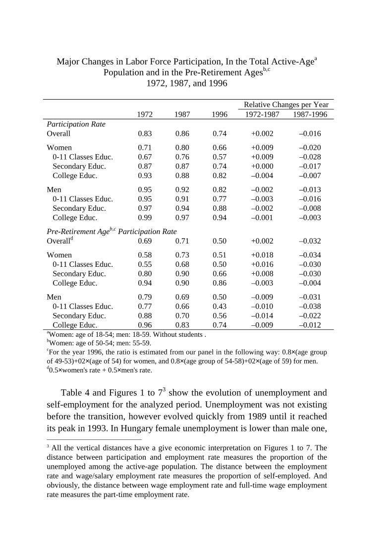
Table 3 and Figure 1 to 7 show the most important trends in labor forceparticipation. Note, that these figures are higher than figures based uponthe standard active age population because mostly non-participant groupsare excluded (full-time students and old-age pensioners), therefore theycannot be compared with other sources.

The tendencies are clear: in the last 15 years before the transition laborforce participation increased. It was due to one direct and one indirecteffect: (1) the increasing participation of low-educated women (2) and(mostly) the increase of average education, because both more educatedmen and women participate more. On the other hand the participation rateof all educational groups of men and highly educated women started todrop before the transition.

However the transition brought about a rather dramatic fall in overallparticipation. The participation rate fell for all educational groups of menand women. Low-educated women experienced the most dramatic drop.The decline has stopped for men by 1993, while for women it has stoppedonly around 1995.

Table 3

Major Changes in Labor Force Participation, In the Total Active-Agea

Population and in the Pre-Retirement Agesb,c

1972, 1987, and 1996

Relative Changes per Year1972 1987 1996 1972-1987 1987-1996

Participation RateOverall 0.83 0.86 0.74 +0.002 –0.016

Women 0.71 0.80 0.66 +0.009 –0.020 0-11 Classes Educ. 0.67 0.76 0.57 +0.009 –0.028 Secondary Educ. 0.87 0.87 0.74 +0.000 –0.017 College Educ. 0.93 0.88 0.82 –0.004 –0.007

Men 0.95 0.92 0.82 –0.002 –0.013 0-11 Classes Educ. 0.95 0.91 0.77 –0.003 –0.016 Secondary Educ. 0.97 0.94 0.88 –0.002 –0.008 College Educ. 0.99 0.97 0.94 –0.001 –0.003

Pre-Retirement Ageb,c Participation RateOveralld 0.69 0.71 0.50 +0.002 –0.032

Women 0.58 0.73 0.51 +0.018 –0.034 0-11 Classes Educ. 0.55 0.68 0.50 +0.016 –0.030 Secondary Educ. 0.80 0.90 0.66 +0.008 –0.030 College Educ. 0.94 0.90 0.86 –0.003 –0.004

Men 0.79 0.69 0.50 –0.009 –0.031 0-11 Classes Educ. 0.77 0.66 0.43 –0.010 –0.038 Secondary Educ. 0.88 0.70 0.56 –0.014 –0.022 College Educ. 0.96 0.83 0.74 –0.009 –0.012aWomen: age of 18-54; men: 18-59. Without students .bWomen: age of 50-54; men: 55-59.cFor the year 1996, the ratio is estimated from our panel in the following way: 0.8×(age groupof 49-53)+02×(age of 54) for women, and 0.8×(age group of 54-58)+02×(age of 59) for men.d0.5×women's rate + 0.5×men's rate.

Table 4 and Figures 1 to 73 show the evolution of unemployment andself-employment for the analyzed period. Unemployment was not existingbefore the transition, however evolved quickly from 1989 until it reachedits peak in 1993. In Hungary female unemployment is lower than male one, 3 All the vertical distances have a give economic interpretation on Figures 1 to 7. Thedistance between participation and employment rate measures the proportion of theunemployed among the active-age population. The distance between the employmentrate and wage/salary employment rate measures the proportion of self-employed. Andobviously, the distance between wage employment rate and full-time wage employmentrate measures the part-time employment rate.

which is a rather unique feature of the Hungarian labor market. This iseasy to explain if we observe that participation declined more amongwomen that among men, therefore since women (may) have better outsideopportunities they rather opted for exiting from the labor market, whilemen rather stayed in the labor market and searched for new employment.

Table 4Major Changes in Unemployment and Self-Employmenta

1972, 1987, and 1996

Relative Changes per Year1972 1987 1996 1972-1987 1987-1996

Unemployment RateOverall 0.00 0.00 0.10 – –

Women 0.00 0.00 0.09 – – 0-11 Classes Educ. 0.00 0.00 0.12 – – Secondary Educ. 0.00 0.00 0.08 – – College Educ. 0.00 0.00 0.02 – –

Men 0.00 0.00 0.11 – – 0-11 Classes Educ. 0.00 0.00 0.14 – – Secondary Educ. 0.00 0.00 0.07 – – College Educ. 0.00 0.00 0.03 – –

Self-Employment Rate (Among the Employed)Overall 0.15 0.15 0.26 +0.003 +0.082

Women 0.14 0.12 0.21 –0.007 +0.072 0-11 Classes Educ. 0.18 0.16 0.23 –0.008 +0.050 Secondary Educ. 0.02 0.09 0.20 +0.193 +0.131 College Educ. 0.02 0.03 0.14 +0.069 +0.341

Men 0.15 0.17 0.31 +0.012 +0.086 0-11 Classes Educ. 0.18 0.20 0.32 +0.007 +0.071 Secondary Educ. 0.05 0.15 0.32 +0.129 +0.131 College Educ. 0.05 0.11 0.25 +0.079 +0.147

The case of self-employment is rather complicated. Between 1972 and1987 we cannot see much change. However it can be surprising that evenin 1972 15 percent of total employment was self-employed. This is due tothe fact that we considered the members of agricultural cooperatives asself-employed. We had several reasons for doing that: they had somefreedom for their agricultural activities (they had some land for their

individual use, they were growing and selling animals), they were notemployees legally, and finally the compensation schemes in thecooperatives were very different from wage/salary schemes. Nevertheless,in no way we claim that they were (with the few exceptions of themembers of some “special” cooperatives) sole proprietors.

We conjecture that there were important changes behind the observedstagnation in the level of self-employment before the transition. We knowthat there was a shift from agriculture to the other sectors to the economyduring the 70’s and 80’s. At the same time during the 80’s theopportunities for small businesses increased in a great extent. Thereforethe underlying sectoral composition and the major characteristics of self-employment might change significantly between 1972 and 1987.

During the transition period the incidence of self-employmentincreased sharply. The increase was higher among men and among thehigher educated. This tendency indicates, that the higher level of self-employment this time is reflecting the development of small privatebusinesses. However we have to note that one of the most common way ofavoiding the payment of the tax burden of salaries is to employ the sameperson as a sole proprietor with a business contract instead of employingher as an employee with a labor contract. This practice led to the increaseof self-employment as well.

The Figures show that in the case of each group the proportion of full-time wage/salary employment was decreasing among the active agepopulation. This decline was due to the decline in participation, to theoccurrence of unemployment and to the increasing self-employment. Onthe other hand part-time employment did not change significantly. This isimportant because our earnings measure refers to the full-time wage/salaryemployment. However this definition covers much smaller proportion ofthe active age population after the transition. We have lower representationof the low educated (they participate less in the labor force and suffer fromhigher unemployment rates), and at the same time we have also less highlyeducated because of the increase in self-employment. We can expect thatthose with lowest productivity are the ones who are leaving the labor force(or losing their jobs), while those with highest productivity are the ones

who become entrepreneurs. However both of these factors implies thatceteris paribus the observed wage/earnings inequality should decline (welose people from the lower and upper tail of the earnings distribution).

Table 5Major Changes in Relative Earnings (Average of the Year = 1),

1972-1987 and 1986-1996

Relative Changes inRelative Earnings, per Year

1972 1987 1986 1996 1972-1987 1986-1996By Education 0-11 Classes 0.93 0.90 0.91 0.79 –0.003 –0.015 Secondary 1.04 1.02 1.00 1.05 –0.001 +0.006 College 1.54 1.43 1.43 1.63 –0.005 +0.015By Gender Women 0.79 0.84 0.84 0.91 +0.004 +0.009 Men 1.15 1.13 1.12 1.08 –0.001 –0.004By Age 25-34 1.01 0.94 0.94 0.93 –0.004 –0.001 35-49 1.10 1.08 1.09 1.04 –0.001 –0.005 50-59 1.16 1.18 1.16 1.18 +0.001 +0.002By Gender and EducationWomen 0-11 Classes 0.73 0.73 0.73 0.68 –0.001 –0.008 Secondary 0.86 0.90 0.87 0.97 +0.003 +0.013 College 1.19 1.18 1.19 1.36 –0.001 +0.016Men 0-11 Classes 1.06 1.01 1.01 0.85 –0.003 –0.018 Secondary 1.22 1.18 1.17 1.16 –0.002 –0.001 College 1.72 1.64 1.60 1.90 –0.003 +0.021

Table 5 and Figures 8 to 12 show the evolution of real net earnings andrelative net earnings. Real net earnings were declining since 1977,however this decline was accelerated sharply by the transition. The onlyexception is the 1992-1994 period, however the stability of real earningswas rather due to an “election budget” than economic development.

Before studying the pattern of relative earnings it is worth noting that(with respect to relative earnings) there is no significant difference by the1986 and 1987 figures. It is important because, as pointed out in theprevious section, the data for these two years are coming from two

different sources (from the NLC WS for 1986 and from the CSO IS for1987). These results therefore justify the use of the two sources in a unifiedframework.

Focusing on relative earnings by education, it seems that there were noimportant changes before the transition. The differentials were ratherconstant, although there was a slight tendency towards the narrowing ofthe educational differences. The transition brought about considerablechanges. The relative earnings of low-educated employees fell sharply,while the ones with college degree gained in relative terms. Both changewas sharper in the case of men than in the case of women. This indicatesthat the transition brought technological change, which favors skills, sinceat the same time the share of skilled labor among employment alsoincreased. (See the last section for more about the role of labor demand inthe transition.)

The raw measure of male-female earnings differential decreased from21 to 9 percent. This decrease is partly due to the decreasing gap for mosteducational groups but also to the previously observed fact that womenbecame more educated during the analyzed period. The role of thecomposition effect is highlighted by the fact that in 1996, the wagedifferential by educational groups is between 28 percent (for college) and16 percent (for secondary degree), all higher than the overall differential.

On the other hand we cannot see too much movement with respect toage: the (aggregate) earning differentials of different age groups wererather stable. The only significant change was the 7 percentage pointsdecline of the relative wage of the 25-34 year age group between 1972 and1986.

Finally, we can follow the dispersion of earnings in Table 6 and onFigures 13 and 14. The first observation we can make that the dispersionwas rather constant in time before the transition with the importantexception of low-educated women, for whom it was decreasing a lot. As itis expected, it was increasing with age. Also as expected, it was increasingwith education in the case of men. However in the case of women we canobserve the opposite direction: the dispersion was rather decreasing with

education. We do not have a clear explanation of this feature of thesocialist labor market. One explanation can be that highly educated womenduring the socialism were mostly employed by the public sector(education, health and public administration) where wage setting wasextremely rigid. However this is not explaining the fact that wages ofwomen with 0 to 11 classes have much higher wage dispersion than menwith the same educational level.

Table 6Major Changes in the Relative Dispersion (Std. Error/Mean) of Earnings,

1972-1987 and 1986-1996

Relative Changes in RelativeDispersion, per Year

1972 1987 1986 1996 1972-1987 1986-1996Overall 0.48 0.47 0.44 0.73 –0.001 +0.071By Education 0-11 Classes 0.46 0.42 0.39 0.50 –0.007 +0.033 Secondary 0.43 0.42 0.41 0.55 –0.002 +0.037 College 0.55 0.57 0.54 0.90 +0.003 +0.076By Gender Women 0.57 0.43 0.46 0.64 –0.016 +0.045 Men 0.43 0.47 0.44 0.77 +0.005 +0.083By Age 25-34 0.35 0.42 0.41 0.63 +0.014 +0.060 35-49 0.44 0.47 0.45 0.72 +0.005 +0.067 50-59 0.47 0.55 0.54 0.82 +0.011 +0.060By Gender and EducationWomen 0-11 Classes 0.65 0.50 0.48 0.60 –0.015 +0.029 Secondary 0.43 0.42 0.38 0.50 –0.003 +0.034 College 0.37 0.41 0.39 0.73 +0.006 +0.095Men 0-11 Classes 0.38 0.37 0.35 0.45 –0.001 +0.033 Secondary 0.42 0.42 0.42 0.58 +0.000 +0.042 College 0.57 0.62 0.58 0.96 +0.005 +0.074

The transition brought about a sharp increase in the dispersion ofearnings for all groups. It also widened the gap between differenteducational and age groups (the case of women still remained puzzling). A

new phenomenon is that now there is a significant difference between thedispersion of men’s earnings and women’s earnings.

Figures 13 and 14 approach the question of earnings dispersion fromanother viewpoint. How much of the dispersion of the earnings can beexplained by gender, education and age (“between-group inequality”) oralternatively, how big is the role of another factors not captured by ourcell-defining variables (“within-group inequality”)? We found that beforethe transition not only the dispersion of earnings but also the“composition” of this dispersion was rather constant, and within groupvariation was responsible about 60 percent of total variation. After thetransition all measures of variation increased, however the within groupvariation did so the most. Here we have to note again, that by the transitionmostly people from the lower and perhaps the upper tail of the earningsdistribution dropped from the sample of full time wage/salary workers.This may bias downward the extent of the importance of these dimensionsas determinants of overall inequality. Nevertheless, the conclusion thatafter the transition other characteristics than gender, education and agebecame increasingly important seems to be robust.

4. DECOMPOSING THE TRENDS IN EARNINGS: A PANELANALYSIS

So far, we did not use the panel nature of our database. In what follows, weexploit that in a simple decomposition of the earnings trends. A similarprocess is discussed in Deaton (1997), Chapter 2.7, also on cohort-aggregated time series of cross-sections. We estimate a regression modelby education levels, with fixed effects for cohort, year and year-genderinteraction and with a 2nd order polynomial in labor market experience.This allows us to decompose the changes in real net earnings into cohort-(or vintage-) and year-effects, estimate the time path of the gender earningsgap, and estimate the experience-earnings profile in a longitudinal setup.

We estimate the following model:

wcgst = γcs + θst + δgst + αs expcgst + βs exp2cgst + εcgst

where index c refers to the different cohorts (that is, vintage), g to gender(1 being female), s to schooling attainment (our usual 3 categories), and tto time. wcgst is the average earnings in cell cgs at time t. γcs is cohort fixed-effects, θst is year fixed-effect, δgst is gender-year interaction effect. Withthis specification, δgst measures the trends in the inter-gender earningsdifferences, or the changes of the earnings (wage-) gap. expcgst is potentiallabor market experience, estimated in the usual way (age, which here is theage in the middle of the cohort, minus 6, minus 9, 12 or 16, depending onschooling level). In what follows, we use age and labor market experiencein an interchangeable way. εcgst is the error term.

The estimation of the effects of labor market experience is subject toimportant identification problems. In a cross-sectional sample, it isimpossible to distinguish between cohort (that is, vintage) and age effects.An estimated cross-sectional age-earnings profile shows two main effects:that of labor market experience and that attributed to the cohortsthemselves. If, for example, the knowledge people acquire in schoolimproves over time, the younger cohorts start with a better endowment ofhuman capital, which makes their initial (and subsequent) wages higherthan that of the former cohorts experienced. This phenomenon would leadto a flatter profile in cross-section than in longitudinal analysis, becausethe latter estimates the individual paths that are not directly contaminatedby the improvement in schooling. The longitudinal approach would lead toan unbiased estimate of the true experience-earnings profiles, whatevertheir theoretical content is.

Unfortunately, things are a little bit more complicated. Cohort-specificdifferences can have two different effects: instead of simply "shifting" theprofiles upward, they can change its slope, too. The longitudinal age-earnings profiles can change because of three effects. (1) Somethinghappened to everybody's wage at that particular point of time (a shift to allwages at time t: year effects). (2) The different cohorts have differentinitial endowment when entering the labor market and this increases theirwage throughout their career (a shift of the profile in the different cohorts:cohort fixed-effects). (3) The different cohorts experience different growthrates along their age-earnings profile (different slopes for different cohorts:

cohort growth effects). In a longitudinal context, one can estimate only twoof the three effects. We have chosen to estimate the first two, therefore thefixed, cohort (and year) independent age (experience) effects.4

Our model is a little bit more restrictive and, in the same time, a littlebit richer than what one would expect from a decomposition exercise (see,for example, Deaton, 1997). Instead of estimating fixed age-effects, we puta quadratic restriction on our age variable (measured as potential labormarket experience). On the other hand, we allowed for gender and yearinteraction. In our sample, there is a clear trade-off between the interactionand the fixed age-effects specifications: even in this specification, we have99 coefficients for the 501 observations. As the results show, there arenon-trivial changes in the gender differences through time, so omitting theinteraction would contaminate the other results. Moreover, the quadraticspecification in potential experience is standard in the earnings functions,therefore this allows us to compare our results to other estimates.

We have chosen a graphical representation of the results, because ofthe large number of the estimated parameters. The point estimates of thespecification with real wage (as opposed to log wage) on the LHS areplotted by education level in Figures 15-18. By construction, the estimatedcoefficients measure changes in earnings, and every change is normalizedto 0 in 1972, the base year. Wages (i.e. earnings) are in 1989 terms.

The year-effects (Figure 15) show a mild decreasing trend of realearnings in the 1980s, followed by a dramatic decline during the transition,from 1987. One can also detect some of the swings of the Hungarianmacroeconomic policy, such as the increase of real wages about 1994, andthe effect of the 1995 correction. The time trend is basically the same inthe different education groups. The gender gap (Figure 16) estimates implya very similar trend than what the overall aggregates of the raw data show(Figure 10), except for the highest schooling levels. The 1980s and thetransition experienced a steady decrease in the wage-advantage of men, forthe secondary school and less educated. On the other hand, the gender gapdid not change much for the college educated employees. The share of 4 That's why the α-s and the β-s don't depend on c or t. The first to encounter thisidentification problem were Weiss and Lillard (1978), in an individual panel context.

college-educated women in the labor force increased faster than that ofmen during the whole period, while the increase of secondary-schooleducated women became smaller. In the same time, the participation rate ofwomen dropped much faster among the secondary school and lesseducated. Therefore, the decreasing gender gap might be partly explainedby changes in labor supply. Namely, less productive women probably leftthe labor force in a greater extent (however these supply changes wereendogenous).5

Figure 17 and 18 present the cohort effects, the first of the twoshowing the fixed-effects themselves, the second one the year-to-yeardifferences. The cohort effects are increasing, in a monotone andsignificant fashion. The more educated gain more by the cohort effect.Figure 18 shows more clearly the growth rates and the inter-groupdifferences in them. The fixed cohort-effects increase more for oldestcohorts than the ones that were born right before or after World War 2. Themost interesting phenomenon, however, is the dramatic increase in thegains for those born after the mid-1960s, especially in the case of the moreeducated. Kertesi and Köllô (1999b), and Kézdi and Köllô (2000) attributethe decrease in the slope of the cross-sectional age-earnings profiles tounobserved cohort-effects. From a slightly different angle, it is the samephenomenon we observe here.

Figure 19 shows our longitudinal estimates of the experience-earningsprofiles, in relative terms. The profiles show the familiar concave pattern,with higher slope for the more educated at each point of time. They do nothave a decreasing part. In fact, the profiles do not even "flatten out"towards retirement. There are two reasons why this might happen. First,the lower employment rate for older cohorts (especially during thetransition) results in a selection bias when comparing wages throughoutthe life cycle. Second, implicit employer-employee contracts might alsohave a role. Note that the American literature relates the fact that profiles

5 The large fluctuations in the college-group might result from both data error or real lifechanges. The latter explanation is supported by the relative smoothness of all otherparameters and the fact that the transition was accompanied by rather high volatility inthe real wages of public employees, most of them being women.

were found steeper than thought before to these kind of contracts, asopposed to simple selection bias (see, for example, Lumsdaine andMithcell, 1999). In addition to the standard arguments, there is anotherrational for the existence of implicit contracts in our case. Throughoutmost of the period, the Hungarian pay-as-you-go pension system used tofocus only on the earnings from the last years when calculating pensions.

Our estimates of the age-earnings profile are a lot steeper than thoseidentified by cross-sectional differences. For comparison, we estimated amore restricted model: instead of fully interacting schooling level with alleffects, we constrained all effects to be the same, except for an education-specific intercept. Figure 20 presents the profile estimated this way,together with a cross-sectional estimate for 1989 by Kertesi and Köllô(1999b). As we pointed out, the cross-sectional estimates do not measurethe real life-cycle growth of earnings when vintage effects are present.Technically, the cross-sectional estimates are smaller because they cannotinclude the cohort effects, which, if increasing, are negatively correlatedwith age. In addition to this problem, estimates can be biased for otheromitted variables. Even our longitudinal estimate suffers from this problemin the restricted model of Figure 20: the estimated profile is below all ofthe ones shown in Figure 19, although it is supposed to be an average ofthem. This indicates that the restriction to common effects (especiallycommon cohort-effects) in all schooling groups creates negativecorrelation between the profile and the error term. If, moreover, ignoringobserved heterogeneity (schooling level) has similar effect than ignoringunobserved heterogeneity, the same argument implies that even theseparately estimated profiles are biased downward.

All of this does not mean that quasi-panel models are superior to thecross-sectional ones in every respect. Indeed, a lot of variation is lost inour analysis that is very important in determining earnings. Moreover,selection bias might distort the longitudinal estimates, just like the cross-sectional ones. In an aggregate quasi-panel setup, it is even more difficultto control for this bias. Finally, it is even more important to remember thatour estimates are counterfactual: they are "cleaned" from year effects.Employees themselves don't experience the steep increase in earnings ifyear-effects are negative, as it is the case from the 1980s on.

5. CHANGES IN EARNINGS AND LABOR SUPPLY: A SIMPLEPANEL ANALYSIS

In this section, we focus on the joint changes in wages and labor supply, inour quasi-panel context. We think of this estimation as a partialequilibrium comparative static exercise. That is we look at each (price,quantity) realization, and try to recover some patterns from the jointchanges. We use the term equilibrium routinely, but without implyinganything about whether markets actually clear. Moreover, although atsome points we argue that the changes we see are caused more by demand-or supply-side changes, we basically follow a reduced-form approach. Thatis, we do not specify structural relationships (in any sense of the word).That is, from this analysis, we are not able to tell what happened to labordemand or labor supply. Instead, we can compare the resulting (price,quantity) points. Our question basically is whether prices and quantitiesmoved the same or opposite direction in certain periods, and how strongwas their relation. We try to argue about the possible factors behind thechanges from this information.

Let c denote cohort, i the gender×education groups (i=gs in thenotation of the previous section), and t time. Also, let lnwcit denote the logof net real wages, and lnscit denote the labor supply or employment ofgroup i of cohort c at time t. We measure scit in four different ways: (1)total employment plus unemployment (labor supply: labor forceparticipation), (2) the number of wage/salary employees plus theunemployed (labor supply: participation in the market of wage/salaryemployees), (3) total employment, and (4) wage/salary employment. Weestimate the model with each left-hand-side variables.6 The basic ideabehind these distinctions is the possible distinction between supply anddemand (1&3 vs. 2&4) and the possible dual nature of the labor market

6 scit is number (as opposed to fraction). To avoid variation in it due to sampling errorother than that in the fractions themselves (participation rate, self-employment ratio), wemeasure scit as the corresponding fraction at time t times the sample-median cell size.

(1&2 vs. 3&4). Obviously, when focusing on labor supply in this setup, thesupply decision is reduced to labor force participation (and self-employment). We divide our sample into a pre-transition and a transitionpart (1972-1987 and 1987-1996, respectively). The difference betweenparticipation and employment is unemployment, which was zero before1989, therefore the two are not distinguished in the pre-transition analysis.We estimate the following model in the two subsamples:

lnscit = αci + βi lnwcit + εcit

αci are the group (cohort×gender×schooling) level fixed effects, whileβi is the percentage change in participation or employment, correspondingto a one percent change in earnings. It is tempting to interpret thiscoefficient as an elasticity, but our approach does not imply what kind ofelasticity it would be. There are two issues involved: that of equilibriumand that of reduced form. The first issue is the validity of the comparativestatic interpretation, and it is related to the nature of unemployment.Therefore it can be analyzed by looking at differences in participation andemployment. The second issue is about identification of changes in supplyand demand. Let us focus on the latter one first.

If labor supply changes only because of exogenous, that isdemographic or other non wage-related factors, then βi identifies the long-run elasticity of labor demand for group i. If, on the contrary, changes inquantities are caused solely by the changes in wages, then it is the long-runelasticity of labor supply. Unfortunately, in our case, neither of theseassumptions can be made.7 There are certainly autonomous, life-cycle 7 Freeman (1979), and Katz and Murphy (1992) analyze a similar problem in a differentsetup: they look at how demographic shocks affect wages of a given age-group in theU.S. Katz and Murphy (1992) argue that the cross-time variation in the size of the age-schooling groups can be treated as exogenous to what happens on the spot market forlabor. This variation, therefore, identifies the slope of the aggregate labor demand curve.Even if this strategy can be justified for their case, it would not work for us. Weobserved large structural changes in participation within any age group and within anycohort: the transition experienced increasing non-participation and entrepreneurship.Therefore, it seems that a large part of the cross-time variation of participation in agiven age group is endogenous to what happens on the labor markets.

related changes in the participation rate within a group (defined bycohort×gender×schooling), and the size of those groups certainly affectstheir wages. On the other hand, we have no reason to rule out thepossibility that participation decisions are made endogenously.8

Our aim is, therefore, more modest. If the observed correlation isnegative, then we cannot rule out that only exogenous supply changescaused all the movement on the labor market. In the opposite case, thishypothesis can be rejected. Indeed, one might think that negativecorrelation implies that exogenous labor supply factors dominated themarket, while positive correlation implies that it is labor demand thatplayed the dominant role. The more significant the co-movements are, themore reasonable is this argument.

The above reasoning makes sense in a comparative equilibriumframework with upward sloping supply curves and downward slopingdemand curves. On the other hand, it is not easy to think in terms ofequilibrium if there is a gap between participation and employment. Itturns out, that this problem does not influence the argument much. This isthe result of the nature of the transition unemployment. In addition tojustifying the conclusions of the comparative statics, we can get someadditional insight of what happened in Hungary by distinguishingparticipation and employment.

The sharp increase in unemployment during the transition indicateslarge shocks to labor demand. This shock probably had cyclical andstructural elements: the collapse of the soviet-led trade system implies thefirst one, privatization, new competitive environment and technologyimport the second one. Structural shocks result in structuralunemployment, cyclical shocks in cyclical unemployment. Therefore, onecan assess the relative importance of the two by focusing on the nature ofunemployment.

8 Indeed, by choosing cohorts as opposed to age groups, we maximize the endogenouspart of the within-cohort variation of labor supply.

If unemployment is largely structural, then workers with unmatchedskills get discouraged and give up looking for a job. Therefore, theybecome non-participants. The unemployed are in large part those that didnot give up yet but otherwise are similar to the ones that became non-participants. In this case, the equilibrium quantity on the labor market isclose to actual employment. A structural change in labor demand leads tolower wages and lower employment of the group with the wrong skills.Those displaced sooner appear as non-participants at a given point of time,and those displaced later appear as unemployed. This story implies strongco-movement of wages and employment, and wages and participation, too,the second being slightly weaker because of the adjustment. On the otherhand, if unemployment is cyclical, smaller proportion of the unemployedgive up finding a job, and they probably search longer. Therefore, while asimilar co-movement is expected between employment and wages, that ofparticipation and wages should be significantly smaller. In our notation, ifβi is positive and only slightly larger when the left-hand side variable isemployment, structural shocks are likely to be responsible for things. If βi

is significantly smaller in the second case, however, cyclical componentsare probably very important, too.

We estimate the within- (fixed-effect) and the between estimates of βi,in two subsamples (pre-transition and transition) with two LHS variables(standard labor supply and without self-employment). Let the Asuperscripts denote within-group average, and D superscripts the deviationfrom it: xA

ci= T-1∑t=1T xcit , xD

ci= xcit– xAci. Then, the within- and the

between estimators are estimated by the following equations, respectively:

lnsDcit = βi lnwD

cit + εDcit

lnsAci = αci + βi lnwA

ci + εAci

The within-estimator measures the co-movement of earnings andparticipation/employment for a given group. The between-estimatorcompares the group-averages. The first, therefore, measures how a givengroup of people change their participation as earnings change, or how

earnings change as participation varies. It is independent of cohort, genderand schooling effects, and also the size of the particular group, but not oflife-cycle patterns and year effects. The second is a more complexmeasure: it focuses on differences independent of life-cycle variation oflifetime earnings and total lifetime participation/employment. It mixescohort, gender and schooling effects, and is influenced by the relative sizeof the different groups, and year-effects, too. Note that the variation of thevariables is considerably smaller in the within-model, therefore itsprecision is smaller.

We had to face a problem coming from the aggregate nature of ourdata. Both the LHS and the RHS variable are sample estimates, thereforeboth suffer from measurement error. The measurement error in lnscit leads"only" to inefficiency, and this cannot be cured. On the other hand, theparameter estimates are biased toward zero because of the measurementerror in wages. In the between-estimator, this bias is negligible given ourprecision of the aggregate estimates (see the Data section). However, in apanel model this problem can be serious even if the errors are relativelysmall. The reason is mainly the smaller variation in the differencedvariables. We estimated the measurement-error bias of our estimates, andwe found that the bias is not significant: it is always below 10 per cent ofthe parameter estimates. Se the Appendix for the details.

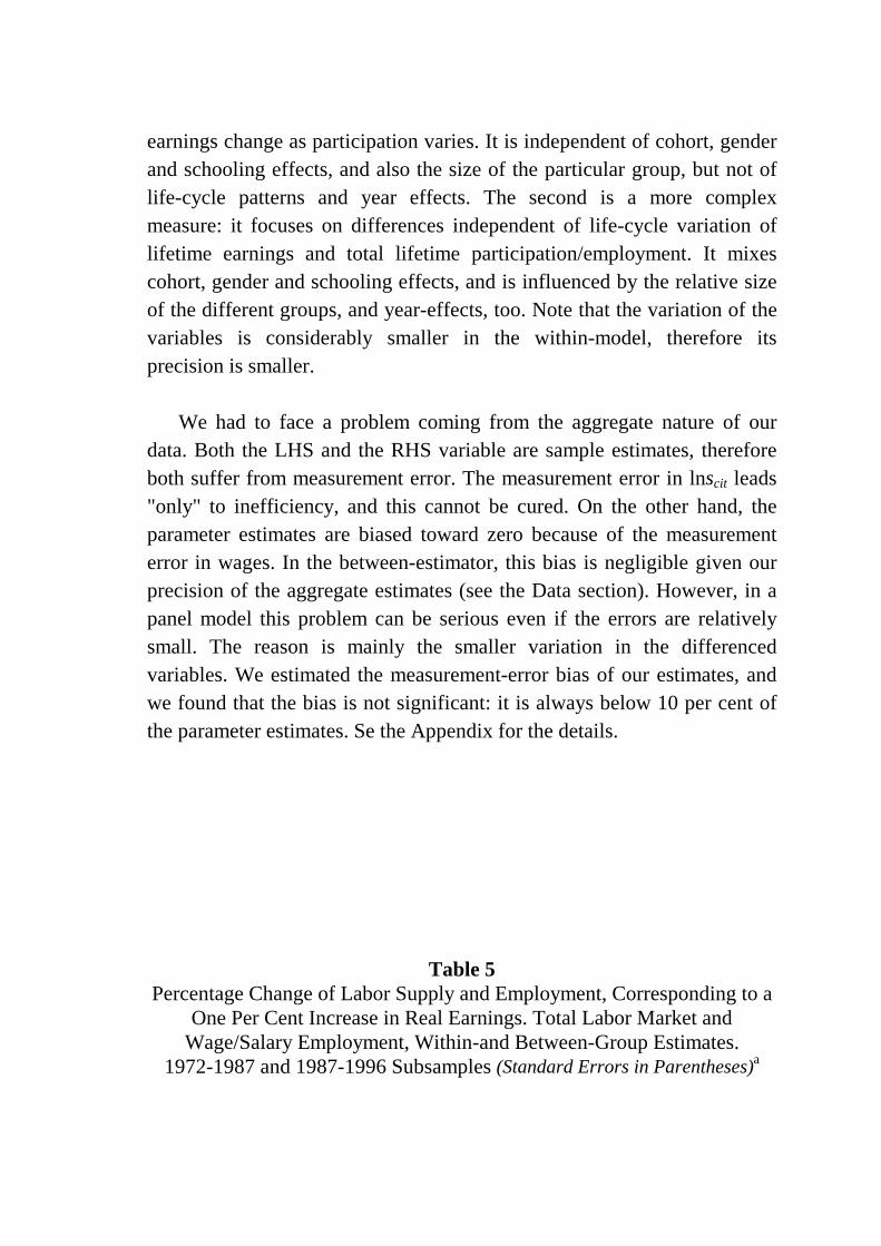
Table 5Percentage Change of Labor Supply and Employment, Corresponding to a

One Per Cent Increase in Real Earnings. Total Labor Market andWage/Salary Employment, Within-and Between-Group Estimates.

1972-1987 and 1987-1996 Subsamples (Standard Errors in Parentheses)a

1972-1987 1987-1996Participation Participation Employment

Within Between Within Between Within Between

Labor Force Participation and Total Employment

Women,0-11 Classes

0.17(0.14)

–1.01(0.27)

0.53(0.13)

1.14(0.43)

0.69(0.15)

1.45(0.47)

Women,Secondary School

–0.07(0.10)

–1.10(0.27)

0.43(0.21)

1.07(0.41)

0.49(0.23)

1.38(0.45)

Women,College

–0.03(0.10)

–1.17(0.26)

0.11(0.25)

0.95(0.40)

0.15(0.28)

1.25(0.43)

Men,0-11 Classes

–0.06(0.11)

–0.95(0.26)

0.60(0.11)

1.14(0.41)

0.77(0.12)

1.44(0.45)

Men,Secondary School

0.01(0.09)

–1.09(0.26)

0.47(0.16)

1.00(0.40)

0.54(0.18)

1.30(0.44)

Men,College

–0.07(0.09)

–1.10(0.25)

0.55(0.22)

0.93(0.39)

0.56(0.25)

1.21(0.42)

Participation and Employment on the Wage/Salary Market

Women,0-11 Classes

–0.07(0.15)

–1.06(0.26)

0.48(0.14)

1.06(0.41)

0.66(0.16)

1.42(0.46)

Women,Secondary School

–0.28(0.10)

–1.13(0.25)

0.43(0.22)

1.00(0.40)

0.51(0.25)

1.36(0.44)

Women,College

–0.07(0.10)

–1.19(0.25)

0.34(0.26)

0.88(0.38)

0.39(0.31)

1.23(0.43)

Men,0-11 Classes

–0.29(0.12)

–1.00(0.25)

0.62(0.11)

1.06(0.40)

0.83(0.13)

1.40(0.44)

Men,Secondary School

–0.27(0.10)

–1.13(0.25)

0.70(0.17)

0.93(0.39)

0.81(0.20)

1.27(0.43)

Men,College

–0.21(0.10)

–1.13(0.24)

0.74(0.23)

0.85(0.37)

0.75(0.27)

1.19(0.41)

aThe parameter and the SE estimates are not corrected for measurement error bias. Thebias is small: for the within-estimator it is around 5-10 per cent of the estimates, for thebetween-estimator, it is around 1 per cent.

The results have a rather clear pattern. Pre-transition estimates arenegative (or cannot be distinguished from zero), while transition estimatesare positive. Within-estimates are always considerably smaller in absolutevalue than between-estimates. Ceteris paribus, male-female differences arenegligible, except for some within-estimates for the transition, andschooling does not change the estimates a lot, either. Note that althoughmeasurement errors bias the within-estimates more than the between-

estimates, their effect cannot explain the large difference. Also, whilewithin-group variation is a lot smaller and thus yields less preciseestimates, the difference between the two is significant. It has, therefore, aneconomic interpretation. In fact, this interpretation is probably different inthe two periods, since the size of the 'elasticity' is different.

The separate treatment of the labor market of wage/salary employmentdid not lead to very different results. With the only exception of the pre-transition within-estimates for men, the estimates are basically the same,and the small differences don't follow any clear pattern. One interpretationof these results is that self-employment does not divide the Hungarianlabor market into very different segments, or if yes, then both were subjectto very similar shocks and both reacted in a very similar way. Therefore, atthis aggregate level, the conclusions drawn based on analyzing thewage/salary market are by and large valid for all employees. On the otherhand, the heterogeneity and the changing composition of the self-employedprevents us to detect significant discrepancies for some sub-groups.

In general, we can conclude that the transition brought about largechanges in labor demand, while the changes in the socialist labor marketswere either driven mostly by exogenous changes in labor supply.9 It shouldbe noted, however, that in this argument 'exogenous' changes in laborsupply are orthogonal to the actual situation but are related to the pastendogenous decisions. For example, this can happen through thedeterminants of schooling level, either by individual choice or centralplanning.

The estimates for employment are larger than those for participation,the difference being (jointly) significant in a statistical sense, notnegligible but also not too large in an economic sense. Labor market

9 Exogenous variation in labor supply is probably much larger between groups thanwithin them. The reason is that it is partly caused by demographic changes andschooling trends, while within-variation is not. We think that the fact that betweenestimates are much more negative in the pre-transition period justifies our conclusion oflabor supply-driven changes, as opposed to the view that pre-transition changes simplycannot be understood in a market equilibrium context.

changes in the transition were, therefore, dominated by structural demandshocks, that were highly correlated with schooling, cohort and gender.

6. SUMMARY: STYLIZED FACTS

At the end of our investigations, we summarize what we think are the mostimportant facts we found. This list of empirical facts can be useful fromdifferent points of view. First of all, it would be important to know whichof them are common regularities across all transition economies (or at leastthe ones similar to Hungary), and which are Hungarian specialties. Second,we think that most of our results are interesting enough in their own to besubject of further investigations. Some of them are puzzling, some of themseem to be common sense. Some of them have been already studied, andsome of them have not. We think that quite a few of them (along with theones that our aggregate analysis could not reveal) should be on the agendaof the empirical research on transition economies. And fourth, themechanisms behind these facts can be also very interesting. Correspondingto this point, theoretical models pursuing to capture the most importantfeatures of the transition from socialism to capitalism should take intoaccount the common facts.

(1) The educational composition of the population improved during thewhole period. Female college education attainment caught up with men'sby 1989. There is a slowdown in the educational improvement trend, bothfor women and men, the latter reaching stagnation. This is not simply theresult of the decreasing size of the entering cohorts, since a similar (ofcourse, smaller) slowdown is true for a particular age group, too.

(2) Before the transition, labor force participation was rather constant forall demographic groups (increasing for lower educated women and slightlydecreasing for men). The transition resulted in a dramatic decline in thelower educated groups, especially among women.

(3) Labor force participation rate of the pre-retirement cohorts followedthe overall average in the 1970s and the 1980s, with somewhat largerincrease in the female rates and larger decrease in the male rates. However,

during the transition, the fall was twice as large as the average, and menexperienced an even larger decline.

(4) Unemployment increased from zero to 13 per cent during thetransition. The resulting unemployment rates vary a lot between educationgroups, but not much between men and women. It seems that low-educatedwomen leave the labor force rather than become unemployed, even morethan men do.

(5) The share of non-wage employment increased throughout the wholeperiod, indicating the increasing importance of entrepreneurship. Thistrend accelerated during the transition. The increase in self-employmentwas much higher for the more educated groups.

(6) Part-time work was not significant in the socialist economy, and it didnot become too important during the transition, either.

(7) Real wages (net earnings) increased in the 1970s, stagnated duringmost of the 1980s, and declined sharply during the transition.

(8) Relative wages did not change much before 1989, with the exceptionof the decrease for highly educated men. The transition brought aboutincreasing differences corresponding to schooling level. The advantage ofcollege-educated employees increased a lot, and the trend seems tocontinue.

(9) The gender gap in earnings decreased slightly in the 1970s, andbecame even narrower during the transition. This trend, however, seems tohave stopped in 1996. The gender gap did not decrease for the collegeeducated.

(10) Overall earnings inequality decreased slightly in the 1970s, did notchange much in the 1980s, and increased dramatically with the transition,especially in the latest years. The level and also the increase is higheramong men and among the more educated.

(11) Only a small part of the increasing inequality is due to the factorsanalyzed above; the most important driving forces are not captured bysimple demographic variables. Within-group variation accounted for morethan three fourths of total variation by 1996.

(12) There is evidence for the positive and accelerating cohort-specificbenefits for the new entrants, especially for those with higher education.This includes those that were already in their early 30s during thetransition. The age-earnings profiles are therefore a lot steeper in alongitudinal setup than they seem in cross-section.

(13) Trends on the labor market were probably dominated by exogenoussupply effects before the transition. These exogenous effects were partlydue to demographic changes, but probably partly due to trends inschooling.

(14) The transition resulted in large shocks in labor demand, whichaffected all groups. These shocks were mostly structural (as opposed tocyclical), and highly correlated with vintage, gender and schooling.Unemployment is structural, and non-participation is closely related to it.

REFERENCES

Deaton, Angus (1997), The Analysis of Household Surveys. AMicroeconometric Approach to Development Policy, Baltimore, JohnsHopkins University Press.

Freeman, Richard (1979), "The Effect of Demographic Factors on Age-Earnings Profiles", Journal of Human Resources, 14(3).

Griliches, Zvi and Hausman, Jerry A. (1981), "Errors in Variables in PanelData", Journal of Econometrics, 31.

Katz, Lawrence F. and Murphy, Kevin M. (1992), "Changes in RelativeWages, 1963-1987: Supply and Demand Factors". Quarterly Journal ofEconomics, Feb.

Kertesi Gábor and Köllô János (1997), "Reálbérek és keresetiegyenlôtlenségek." (Real Wages and Earnings Inequality) KözgazdaságiSzemle, 7-8.

Kertesi Gábor and Köllô János (1998), "Regionális munkanélküliség ésbérek az átmenet éveiben" (Regional Unemployment and Wages Duringthe Transition) Közgazdasági Szemle, 7-8.

Kertesi Gábor and Köllô János (1999a), "Unemployment, Wage Push andthe Wage Competitiveness of Regions -The case of Hungary underEconomic Transition”, Budapest Working Papers On The LaborMarket,1999/5.

Kertesi Gábor and Köllô János (1999b), "Economic Transformation andthe Returns to Human Capital -The case of Hungary 1986-1996”, BudapestWorking Papers On The Labor Market,1999/6.

Kish, Leslie (1965), Survey Sampling. New York, Wiley.

KSH (1981), A keresetek színvonala, szóródása és kapcsolata a családijövedelemmel 1972. és 1977. (Level and Dispersion of Earnings, and TheirRelation to Family Income, 1972 and 1977), Központi Statisztikai Hivatal,Budapest

KSH (1986), "A keresetek színvonala, szóródása és kapcsolata a családijövedelemmel 1982." (Level and Dispersion of Earnings, and TheirRelation to Family Income, 1982), Központi Statisztikai Hivatal, Budapest

KSH (1990), "Jövedelemeloszlás Magyarországon. Az 1988. évi jövedelmifelmérés adatai." (Income Distribution in Hungary. Data from the 1988Income Survey.), Központi Statisztikai Hivatal, Budapest

Lumsdaine, Robin L. and Mitchell, Olivia S. (1999), "New Developmentsin the Economic Analysis of Retirement", Ashenfelter and Card, eds.,Handbook of Labor Economics,Vol. 3. Elsevier, New York.

Weiss, Yoram and Lillard, Lee A. (1978) "Experience, Vintage and TimeEffects in the Growth of Earnings: American Scientists 1960-70." Journalof Political Economy, 86(3) pp. 427-48.

DATA APPENDIX

Data Sources

The data we use come from four different kind of sources. Table A1 showsthe contribution of each type of survey. The following section (with TablesA2 through A4) describes the surveys briefly.

Table A1: Years of the Cells in the Quasi-Panel Data setand the Sources of the Data (Q: labor market "quantity"variables: participation, employment, etc. W: wages)

CSO IS Census1990

CSOLFS

NLCWS

1972 Q,W1977 Q,W1982 Q,W1986 Qa W1987 Q,W1989 Q W1992 Q W1993b Q1994 Q W1995 Q W1996 Q W

aThe employment data in the 1986 cells are estimates, based on linear interpolation of the ratios from the 1982 and 1987 CSO IS.

b There are no earnings data in the 1993 cells.

The CSO IS Data(In Hungarian: KSH Jövedelemfelvétel)The CSO Income Surveys were large independent cross-sectionalhousehold surveys representing the non-institutional population conductedin every five years from 1963 on. The micro data from the 1960s are lost.These surveys are excellent sources of labor market data, since they matchthe demographic information provided by the households with theoccupation and earnings information provided by the employer for eachhousehold-member holding a job. The following table shows the mostimportant information about the samples, the estimated effect of thesample design on standard errors, and the number of the outliers in theearnings data.

Table A2: Sample Information about the 1973, 1978, 1983, and 1988 CSOIncome SurveysYear of Survey 1973 1978 1983 1988Year of Employment Data 1972 1977 1982 1987Year of Earnings Data 1972 1977 1982 1987Sample Size: All Individuals 111,037 a 48,361 43,474 56,439Sample Size: Wage Data 41,009a 17,700 15,947 19,873Non-Response Rate n.a. n.a. 0.02 0.17N. of Labor Force Participantsb 54,374 22,738 19,827 25,773N. of Full-Time Wage Employed 42,291 18,170c 13,591 18,222deff on Employed/Pop.dMean deff on Employed/Pop. per Celld

deff on Overall Mean Earningsd 1.028 1.070 1.072 1.001Mean deff on Cell Mean Earningsd 1.039 1.051 1.032 1.029N. of Outliers in Earnings 19 21 5 76aIn the 1973 sample, the original sample size is 27,048 households, and the records aredoubled for Budapest, and Bács, Borsod, Hajdú and Pest counties.bBecause of full employment in the socialist economy, participation is identical toemployment until 1989.cThere is no full-time status information available in the 1978 data set. The abovenumber refers to total wage employment. In the quasi-panel data set, the ratio of full-time employment to total wage employment is estimated as the average interpolatedratio between 1972 and 1982.ddeff is Leslie Kish's measure of the sampling design effect. It gives the ratio of the truesampling variance of the statistic (here: overall mean and mean of the means in thecells) to the simple random sample-based estimation of the sampling variance. See Kish(1965). The "true" variance here is estimated by bootstrapping, thereforedeff=(VARBOOTSTRAP /VARSRS).

The 1990 Census Data(In Hungarian: Népszámlálás)The CSO conducts a census in every 10 years. We used the information ofthe short questionnaire, which includes everything we needed (schooling,too), except for full-time employment. Our sample was a 2 percent simplerandom sample of the total population, total sample size was thereforeabove 200,000. Non-response was 0, since it is forbidden by law.

The CSO LFS Data(In Hungarian: KSH ELAR Munkaerôfelvétel)The LFS is a quarterly conducted rolling household panel survey of morethan 20 thousand non-institutional households. Each time, one sixth of thesample is replaced, so one household stays for 6 quarters in the sample.One main objective of the survey is to provide accurate, ILO-standardmeasures of participation and unemployment. It also contains rather

detailed information about the employment: sector, occupation, and hoursworked is provided. It is a household survey, so all information come fromthe respondents.

Table A3. Sample Information about the 1992, 1993, 1994, 1995, and1996 CSO Labor Force SurveysYear of Survey 1992 1993 1994 1995 1996Year of Employment Data 1992 1993 1994 1995 1996Sample Size: Total N. ofIndividuals

54,284 61,345 60,791 68,927 64,609

Sample Size: N. of Active-AgeIndividuals

36,222 30,888 30,222 33,185 32,506

The NLC WS Data(In Hungarian: OMK Bértarifa-felvétel)The WS are very large regular (from 1995 on yearly) cross-sectionalsurveys of individual earnings and occupational data, also includinggender, date of birth, and schooling information. The data are collectedfrom the employers on an administrative basis. They represent thepopulation of firms employing more than 20 persons (more than 10 from1995). The sampling design of the firms (and other institutions) includedstratification and no clustering. Within each firm, the individuals were tobe selected by the administration of the firm, based on the day (not monthand year) of birth. The individual sample is therefore not literally random,but the selection criterion is probably orthogonal to any interestingvariable. This way, sample design included more levels, but this did notdecrease the efficiency of the estimates (see the design effects below).

Table A4: Sample Information about the 1986, 1989, 1992, 1995, and1996 NLC Wage Survey DataYear of Survey 1986 1989 1992 1995 1996Year of Earnings Data 1986 1989 1992 1995 1996Sample Size: N. of Full-TimeWage Employed

145,419 145,460 131,677 153,229 160,481

deff on Overall Mean Earningsa 0.999 0.999 1.000 0.999 0.999Mean deff on Cell Mean Earningsa 1.000 1.000 1.000 1.000 0.999aSee the notes in Table A2 for the definition of deff.

The Quasi-Panel Database

The quasi-panel is a collection of groups defined by their cohort (5-yearinterval of date of birth), gender, and schooling level (3 categories: 0-11classes, secondary school, college or more). These groups are followedthroughout the years 1972-1996. Each cohort consists of 6gender×education cells, except for the oldest group (because women'sgeneral retirement age has been just 5 years less than the one of men), andthe youngest one (because the youngest cohort covers the 15-19 years old).The cohort-boundaries are created in such a way that they exactly cover theworking-age population (men: 15-59, women: 15-54 years old) in theearly surveys (note that both the surveys and the cohorts follow each otherin 5 year intervals). Of course, this pattern is not shared by the 1986, 1989,1993-6 years, so they include "truncated" cells as well. We estimated thequantity and the earnings variables in for all truncated cells that containedenough observations in the original surveys. Table A5 shows how thecohorts are represented in each year. Table 6 contains the total number ofobservations in the original data sets that are represented by the quasi-panel, while Table 7 provides cells-based statistics about the size of theoriginal samples.

Table A5: Number of Data cells Per Cohort in a Given Year

Year ofBirth

1972 1977 1982 1986 1987 1989 1992 1993 1994 1995 1996

1913-17 3 0 0 0 0 0 0 0 0 0 01918-22 6 3 0 0 0 0 0 0 0 0 01923-27 6 6 3 3 0 0 0 0 0 0 01928-32 6 6 6 6 3 3 0 0 0 0 01933-37 6 6 6 6 6 6 3 3 3 3 31938-42 6 6 6 6 6 6 6 6 6 6 61943-47 6 6 6 6 6 6 6 6 6 6 61948-52 6 6 6 6 6 6 6 6 6 6 61953-57 4 6 6 6 6 6 6 6 6 6 61958-62 0 4 6 6 6 6 6 6 6 6 61963-67 0 0 4 4 6 6 6 6 6 6 61968-72 0 0 0 0 4 4 6 6 6 6 61973-77 0 0 0 0 0 0 4 4 4 4 41978-82 0 0 0 0 0 0 0 0 2 2 2Total 49 49 49 49 49 49 49 49 51 51 51

Table A6: Total Number of Individual Observations in the Panel

1972 1977 1982 1986 1987 1989Employment Data 60,936 25,700 22,837 – 29,728 101,195

Earnings Data 40,853 17,704 15,385 141,175 17,532 142,357

1992 1993 1994 1995 1996Employment Data 36,222 30,888 30,222 33,185 32,506Earnings Data 129,977 – 151,016 150,671 157,766

Table A7: Number of Individual Observations per Cells in the Panel(Median, 25th Percentile, 5th Percentile, Minimum)

"Quantity" Data Earnings DataMedian 25th P. 10th. P. Min. Median 25th P. 10th. P. Min.

1972 451 264 107 78 421 246 94 661977 267 135 61 40 246 120 59 361982 267 149 62 33 235 113 61 311986 – – – – 2,087 1,248 96 321987 364 212 95 43 281 163 75 241989 1,355 738 264 129 2,300 1,297 361 1061992 573 291 88 41 2,135 1,526 271 431993 506 237 114 67 – – – –1994 447 220 85 58 2,383 1,599 402 191995 507 239 100 61 2,486 1,606 299 591996 436 253 55 31 2,491 1,716 247 139

Definition of The Variables

Population. We included all individuals in the age range of 15-59(women: 15-54) who were not full-time students. This latter requirementnaturally reduces the age-range of the college-educated groups: the lowerbound is in general 24. (See also the section on truncated cells.) Thisdefinition of the population has two shortcoming with respect to the laborsupply decision: for young generations it is (at least to some extent) aneconomic decision whether they are starting to work (or searching for ajob), remain out of the labor force, or studying more. On the other hand,people over the compulsory retirement age still chose to work. In fact, itwas common during the pre-transition period and became very rare afterthe transition. Therefore this definition of the population excluding twoimportant aspects of the labor supply reactions to the transition shock.

Labor force participation, unemployment. Labor-market participationincludes employment and unemployment, and it excludes those that are inthe military service or on child-care leave. (Note that the CSO definitionincludes these two groups.) Unemployment is measured by the ILO-standard set of questions in the CSO LFS, (from the beginning in 1992).

There was no unemployment before 1989, but the year of 1989 isproblematic. As mentioned about, we used the 1990 Census (theoreticaldate of survey: Jan 1. 1990) for measuring the 1989 quantities. The censusasks only about registered unemployment, however in that early stages ofthe transition we can assume that registered and ILO unemployment figurewere very similar.

Wage/salary employment, full-timers. Wage/salary employmentexcludes agricultural co-op employment, sole proprietorship, self-employment, and helping family members. Full-time employment is anexplicit question in the CSO IS (1972,77,82,87) (however the data file didnot contain this variable in 1977). About 10 percent of the variable wasmissing in the other surveys, those we took as full-timers. In the CSO LFS(1992,3,4,5,6) we defined full-timers those that worked at least 36 hoursper week on average, or work less but their job description describes thisamount of work as full-time employment, or they could not tell the average(or told it changes a lot), but they worked more than 36 hours last week.10

The 1990 Census did not contain information about full-time employment,so the corresponding rates for 1989 are interpolated using the 1987 and the1992 figures.

Earnings. The earnings data refer to the full-time wage/salary employed.Earnings is defined as the monthly average of wages and other, work-related payments. In the CSO IS (1972,77,82,87), the earnings data arebased on information from the employer, and they consist of the yearlysum of baseline wages and other work-related payments, divided by thenumber of months worked. See KSH (1981, 1986 and 1990) for moredetails.11 Note that the workplace was the distribution unit of some welfaretransfers in the socialist system, such as child-care benefits, but theearnings data don't contain these components. For the years 1972, 1977and 1982 we used the earnings variable created by the CSO, while for1987, in the absence of the CSO variable, we created it (with the help ofthe CSO staff). The NLC WS earnings data are created by Gábor Kertesiand János Köllô and follow the same logic. See Kertesi-Köllô (1997b) formore details. Besides their (gross) earnings variable, we also used theirestimates for net earnings from 1989 on. (Personal income tax exists in 10 The 1992 LFS is different from the following ones in this set of questions. However, theinformation needed for this definition could be recovered.11 The included components were base salary/wage, bonus, royalty, wage supplement and otherwage and salary components. (in Hungarian: törzsbér, prémium, jutalom, jutalék, bérpótlék(w/o családi pótlék), kiegészítô fizetés, egyéb bérek).

Hungary from 1988. In 1988, the earnings were "grossed up" so that theafter-tax earnings remain the same.) The estimation is based on the yearlypersonal income tax rates. In the absence of other information, nocorrection could be made for tax-deductible items or the amount of othertaxable incomes. The former components would decrease, the latter oneswould increase the average tax (this second is because of the progressivenature of the scheme). We think that the first effect is larger, so the netearnings are probably underestimated from 1989 on.

APPENDIX: ESTIMATING THE MEASUREMENT ERROR BIASIN A FIXED-EFFECT MODEL12

Consider the model we estimate in section 5:

lnscit = αci + βi lnwcit + εcit ,

and the equations estimating its within (or fixed-effect) and between-models:

lnsDcit = βi lnwD

cit + εDcit ,

lnsAcit = αci + βi lnwA

cit + εAcit ,

where xDcit= xcit– xA

ci , the A superscripts denoting within-group average(xA

ci= T-1∑t=1T xcit), and therefore the D superscripts the deviation from it.

Let bW denote the within- and the bB between-estimator for β (in whatfollows, we suppress the subscripts, for notational simplicity).13 Also, letlnwt* and lnst* denote the population value of net real earnings and ourmeasure of labor supply at time t, respectively. Instead of lnwt* and lnst*,we only have estimates for them, lnwt and lnst, respectively. Let ωt = lnwt –lnwt*, and ξt = lnst – lnst*, and δt

2≡E[ωt2], with an average δ2≡T-1∑t=1

T δt2.

Then, the definition of the fixed-effect estimator is:

E[bW] = Cov[(lnwt – lnwA), (lnst – lnsA)] / Var[lnwt – lnwA] = Cov[lnwD

t, lnsDt] / Var[lnwD

t] = Cov[lnwD, lnsD] / Var[lnwD]

E[bB] = Cov[lnwA, lnsA] / Var[lnwA]

where the A superscript denotes averages, the second line for E[bW] definesthe difference with the D-superscript notation, and the third line assumesthat these differences are drawn from distributions with common first twomoments. The expected value of b is the following:

E[bW] = Cov[(lnwt – lnwA), (lnst – lnsA)] / Var[lnwt– lnwA] 12 The estimation of measurement error in panel context was addressed first by Grilichesand Hausman (1981). Here we follow their argument.13 The derivation below focuses on the lnw specification.

= E[(lnw*t – (lnwA)* + ωt – ωA),(lns*t – (lnsA)* + ξt – ξA)] / Var[lnw*t – (lnwA)* + ωt – ωA] = Cov[(lnwD)*,(lnsD)*] / {Var[(lnwD)*] + δt

2 + (δA)2} = Cov[(lnwD)*,(lnsD)*] / {Var[(lnwD)*] + 2δ2 } = β × Var[(lnwD)*] /{Var[(lnwD)*] + 2δ2}

E[bB] = Cov[lnwA,lnsA] / Var[lnwA] = E[((lnwA)* + ωA)),((lnsA)* + ξA)] / Var[(lnwA)* + ωA] = Cov[(lnwA)*,(lnsA)*] / {Var[(lnwA)*] + (δA)2} = Cov[(lnwA)*,(lnsA)*] / {Var[(lnwA)*] + δ2 } = β × Var[(lnwA)*] /{Var[(lnwA)*] + δ2}

The first line for E[bW] follows from the definition of the OLSestimator, the second line is the expansion of the difference operator, andthe third line uses the definition of ξ and ω. The fourth line uses theassumption that the errors are uncorrelated with the measured variables,the errors are also uncorrelated between two points of time (which is true ifthe consecutive cross-sections are all representative samples), and theerrors in w and s are also uncorrelated (which is certainly true when theycome from different surveys). These imply that Var[lnwD] = Var[(lnwD)*]+ δt

2 + (δD)2. The fifth line uses the fact that (δD)2=δt2 if δt

2=δ2, and the lastline uses the consistency of Cov[(lnwD)*,(lnsD)*]/Var[(lnwD)*] for β. Verysimilar arguments lead to the formula for E[bB].14 From this result, we cansee that the bias in E[bW] can be significant even if the relative error(δ/E[(lnwD)*]) is small, as in our case, if Var[(lnwD)*] is small, but E[bB] isnot biased severely. From now on, we focus on the within-estimator.

14 The most fragile assumption we make here is that the measurement error isuncorrelated with the measured variable. In what follows, we use the sampling variancefor δ2, therefore we assume that the only source of error is due to random sampling. Ifthis is true, the zero-correlation condition automatically follows (so does independence).Since all of our earnings data come from the employer, the problem of correlated errorsin self-reported wage data (see e.g. Kézdi, 1998 and Kézdi, forthcoming) is not relevant.On the other hand, we use estimates for the net earnings since the data we have after1988 (from the start of the income tax system) are before-tax figures. We have noinformation about the sign and size of the correlation of "true" earnings and this errorcomponent.

If we assume that the source of error is the fact that the variables weuse are estimates from representative samples, then δ2 is sampling varianceof lnw. We have relatively good estimates for the sampling variance of w(see the first section), which we can use for the correction. Let d = w – w*,so we have estimates for E[d2]. Then, δ2 = E[ω2] = E[(lnw – lnw*)2] ≈E[(w–w*)2/(w*)2] = E[(w–w*)2]/E[(w*)2] = E[d2] / E[(w*)2], where thethird equality follows from the independence of w from the measurementerror. Since E[(w*)2]= E[w2] + E[d2], δ2 = E[d2] / {E[w2] + E[d2]}.Therefore, we can consistently estimate the (limiting) bias of bW andcorrect our point estimates to get consistent estimates for β:

β = E[bW] × {Var[(lnwD)*] + 2δ2} / Var[(lnwD)*] = E[bW] × Var[lnwD] / {Var[lnwD] – 2δ2} = E[bW] × Var[lnwD] / {Var[lnwD] – 2E[d2]/{E[w2] + E[d2]},so

bW×SampleVar[lnwD]/{SampleVar[lnwD]–2E[d2]/{E[w2]+E[d2]}→ βin probability.

That is, the correction factor for E[bW] is

SampleVar[lnwD]/{SampleVar[lnwD]–2E[d2]/{E[w2]+E[d2]}.

FIGURES

Figure 1Labor Force Participation and Employment

Figure 2Labor Force Participation and Employment

Women, 0-11 Classes

Partic ipation Rate Em ploym ent Rate W age Em ployment Rate Full-Tim e W age Em ploym ent Rate

1972 1977 1982 19871989 1992 1996

.4

.5

.6

.7

.8

.9

1

.4

.5

.6

.7

.8

.9

1

Partic ipation Rate Em ploym ent Rate W age Em ploym ent Rate Full-Tim e W age Em ploym ent Rate

1972 1977 1982 19871989 1992 1996

.4

.5

.6

.7

.8

.9

1

.4

.5

.6

.7

.8

.9

1

Figure 3Labor Force Participation and Employment

Women, Secondary School

Figure 4Labor Force Participation and Employment

Women, College

Partic ipation Rate Em ploym ent Rate W age Em ployment Rate Full-Tim e W age Em ploym ent Rate

1972 1977 1982 19871989 1992 1996

.4

.5

.6

.7

.8

.9

1

.4

.5

.6

.7

.8

.9

1

Partic ipation Rate Em ploym ent Rate W age Em ployment Rate Full-Tim e W age Em ploym ent Rate

1972 1977 1982 19871989 1992 1996

.4

.5

.6

.7

.8

.9

1

.4

.5

.6

.7

.8

.9

1

Figure 5Labor Force Participation and Employment

Men, 0-11 Classes

Figure 6Labor Force Participation and Employment

Men, Secondary School

Partic ipation Rate Em ploym ent Rate W age Em ploym ent Rate Full-Tim e W age Em ploym ent Rate

1972 1977 1982 19871989 1992 1996

.4

.5

.6

.7

.8

.9

1

.4

.5

.6

.7

.8

.9

1

Partic ipation Rate Em ploym ent Rate W age Em ploym ent Rate Full-Tim e W age Em ploym ent Rate

1972 1977 1982 19871989 1992 1996

.4

.5

.6

.7

.8

.9

1

.4

.5

.6

.7

.8

.9

1

Figure 7Labor Force Participation and Employment

Men, College

Figure 8Real Net Earnings, Also By Education (in 1989 Hungarian Forints)

College Secondary School 0-11 Classes Overall

1972 1977 1982 19871989 1992 1996

5000

10000

15000

5000

10000

15000

Partic ipation Rate Em ploym ent Rate W age Em ployment Rate Full-Tim e W age Em ploym ent Rate

1972 1977 1982 19871989 1992 1996

.4

.5

.6

.7

.8

.9

1

.4

.5

.6

.7

.8

.9

1

Figure 9Relative Net Earnings, By Education

Figure 10The "Raw" Gender Gap: Relative Net Earnings By Gender

College Secondary School 0-11 Classes

1972 1977 1982 19871989 1992 1996

.5

1

1.5

2

.5

1

1.5

2

Men W om en

1972 1977 1982 19871989 1992 1996

.8

.9

1

1.1

1.2

.8

.9

1

1.1

1.2

Figure 11Relative Net Earnings of Women, By Education

Figure 12Relative Net Earnings of Men, By Education

W om en, College W om en, Secondary School W om en, 0-11 Classes

1972 1977 1982 19871989 1992 1996

.5

1

1.5

2

.5

1

1.5

2

Men, College Men, Secondary School Men, 0-11 Classes

1972 1977 1982 19871989 1992 1996

.5

1

1.5

2

.5

1

1.5

2

Figure 13Relative Standard Deviation of Net Earnings, Within-Group and Between-

Group Componetns

Figure 14Proportion of Between-Group and Within-Group Variation in Net Earnings

Total Relative Stdv. 'W ithin' Relative Stdv. 'Between' Relative Stdv.

1972 1977 1982 19871989 1992 1996

0

.5

1

0

.5

1

W ithin-Group Variation Between-Group Variation

1972 1977 1982 19871989 1992 1996

0

.5

1

0

.5

1

Figure 15Year Fixed Effects on Real Net Earnings

Figure 16The "Cleaned" Gender Gap: Change in the Difference of Male and Female

Salaries, 1972=0 (Year-Gender Interacted Fixed Effects on Real NetEarnings)

1989

Hun

garia

n Fo

rints

0-11 Classes Secondary School College

1972 1977 1982 1987 1992 1996

-10000

-5000

0

5000

-10000

-5000

0

5000

1989

Hun

garia

n Fo

rints

0-11 Classes Secondary School College

1972 1977 1982 1987 1992 1996

-1000

0

1000

2000

-1000

0

1000

2000

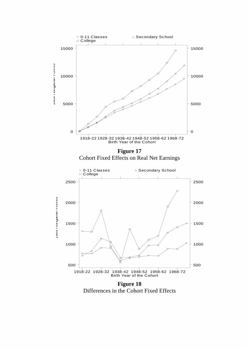
Figure 17Cohort Fixed Effects on Real Net Earnings

Figure 18Differences in the Cohort Fixed Effects

1989

Hun

garia

n Fo

rints

Birth Year of the Cohort

0-11 Classes Secondary School College

1918-22 1928-32 1938-42 1948-52 1958-62 1968-72

0

5000

10000

15000

0

5000

10000

15000

1989

Hun

garia

n Fo

rints

Birth Year of the Cohort

0-11 Classes Secondary School College

1918-22 1928-32 1938-42 1948-52 1958-62 1968-72

500

1000

1500

2000

2500

500

1000

1500

2000

2500

Figure 19Age-Earnings Profiles, Relative Earnings

Figure 20Age-Earnings Profiles, Relative Earnings.

Longitudinal Vs. Cross-Section Estimates (Ours vs. Kertesi & Kollo,1999b, resp.)

Rel

ativ

e C

hang

es

Years of Experience

Longitudinal Decomp. Cross-Section: Kertes i-Kollo

0 10 20 30 40

0

.5

1

1.5

0

.5

1

1.5

Rel

ativ

e C

hang

es

Years of Experience

0-11 Classes Secondary School Classes College

0 10 20 30 40

0

1

2

0

1

2