LONG REPORT FORMAT AND Long and GRADING RUBRIC …

L O N G R E P O R T F O R M A T A N D G R A D I N G R U B R I C

50

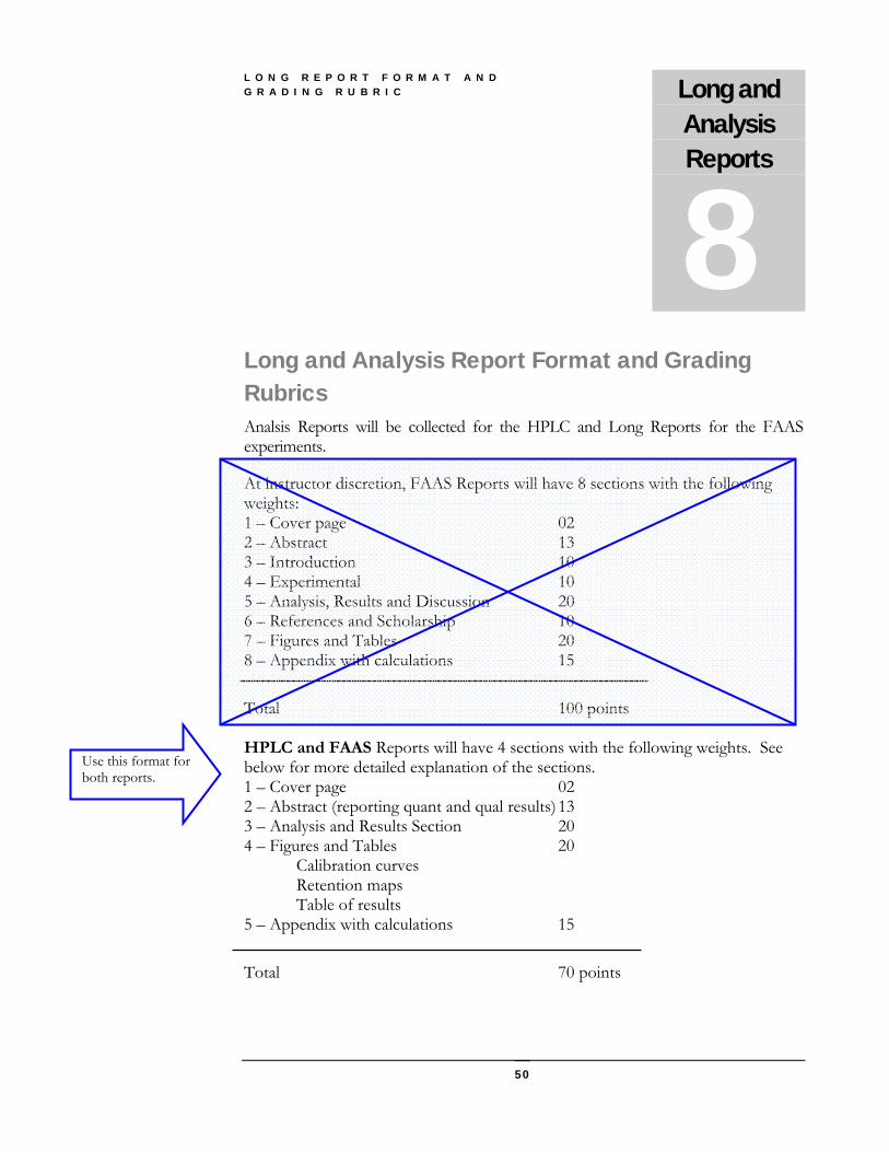
Long and Analysis Report Format and Grading Rubrics Analsis Reports will be collected for the HPLC and Long Reports for the FAAS experiments.

At instructor discretion, FAAS Reports will have 8 sections with the following weights: 1 – Cover page 02 2 – Abstract 13 3 – Introduction 10 4 – Experimental 10 5 – Analysis, Results and Discussion 20 6 – References and Scholarship 10 7 – Figures and Tables 20 8 – Appendix with calculations 15

Total 100 points HPLC and FAAS Reports will have 4 sections with the following weights. See below for more detailed explanation of the sections. 1 – Cover page 02 2 – Abstract (reporting quant and qual results) 13 3 – Analysis and Results Section 20 4 – Figures and Tables 20 Calibration curves Retention maps Table of results 5 – Appendix with calculations 15

Total 70 points

Long and Analysis Reports

8

Use this format for both reports.


51

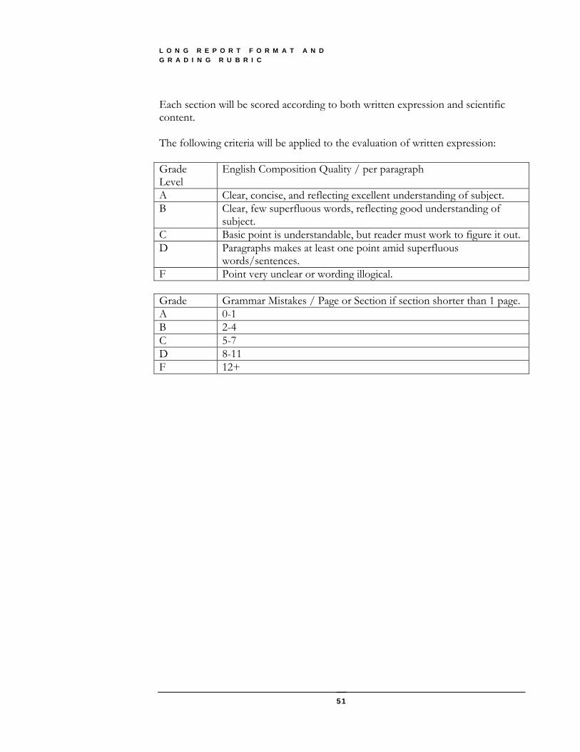
Each section will be scored according to both written expression and scientific content. The following criteria will be applied to the evaluation of written expression: Grade Level

English Composition Quality / per paragraph

A Clear, concise, and reflecting excellent understanding of subject. B Clear, few superfluous words, reflecting good understanding of

subject. C Basic point is understandable, but reader must work to figure it out. D Paragraphs makes at least one point amid superfluous

words/sentences. F Point very unclear or wording illogical. Grade Grammar Mistakes / Page or Section if section shorter than 1 page. A 0-1 B 2-4 C 5-7 D 8-11 F 12+


52

Scientific content and format are summarized below: General remarks: 1. Standard deviations and confidence intervals based on small data sets have two significant figures – not more. The last sig fig in the std dev is the last sig fig reported in the average or calculated answer. Example: 12.23±0.55 = correct

12.23±1.23 = incorrect! should be 12.2±1.2 (last digit = 0.1) 12.2±0.23 = incorrect! should be 12.23±0.23 (last digit = 0.01)

1. Cover page:

1.1. Title 1.2. Your name 1.3. Your partner’s name 1.4. Course 1.5. Professor Terrill 1.6. Date Submitted

2. Abstract: Very, very brief and clear summary of the experiments and results. In a few short sentences convey (a) what was done (measured) and (b) using what method (HPLC or FAAS) and (c) with what crucial conditions and (d) sample preparation and (d) the final results w/ estimated errors (σ and 95% CI) (c). If they were not included in the above, give those few crucial details (λ, stationary phase, mobile phase) that are critical to reproducing the work by an expert and (d) conclusions regarding null hypothesis and bias if possible. 2.1. Length: Approximately 100-200 words. 2.2. Concise description of what was measured and how (method name). 2.3. Results clearly summarized

2.3.1. Zn amt ± error 2.3.2. Fe amt ± error 2.3.3. units of mg/can or mg/pill

2.4. If data quality support conclusions: 2.4.1. Evidence of bias wrt validation? 2.4.2. Evidence of bias wrt expected value? 2.4.3. Evidence of bias from sample to sample?

2.5. Concise description of how measurements made w crucial details only: 2.5.1. HPLC mobile / stationary phases 2.5.2. detection limit / wavelength 2.5.3. FAAS flame type (air / C2H2) 2.5.4. detection limit / wavelength

2.6. Negatives: 2.6.1. Too much detail (raw signals, dilutions, etc.) 2.6.2. Conversational tone or unnecessary words or phrases 2.6.3. Speculation about results

The boxes below contain some key report elements that I use to score the reports!


53

3. Introduction: The tone of an analytical chemistry report where the instrumental method is being developed to solve a particular problem is typically like this: “Compound x is of interest because … The instrumental method yyy is appropriate to this analysis because … In these experiments x was measured (diet Coke™ / Centrum Silver™) with a vvv instrument using zzz conditions. The results were excellent/good/fair/poor (perhaps why). 3.1. Length: Approximately 200-500 words. 3.2. Very short description of the analytes –

3.2.1. what they are 3.2.2. why they are there and 3.2.3. why it is important to quantify them

3.3. Discussion of the instrumental method 3.3.1. how the method works, focusing on the principles of the detection

and/or separation e.g. the absorption of light by gas phase atomic analytes or the partitioning of analytes from a solution (mobile phase) to a stationary phase

3.3.2. why it is appropriate to the problem of measuring this analyte in this matrix – what aspects of this instrumental method make it sensitive or selective for the analytes of interest

3.3.3. possible interferences / problems and how they are controlled or not 3.3.4. description of experimental parameters that are important to this

particular analysis, influence the performance of the instrument and why – e.g. flame stoichiometry or mobile phase composition, wavelength etc.

4. Experimental Methods

4.1. Length: Approximately 50-200 words. 4.2. Instruments and Materials:

4.2.1. List the name and manufacturer of the instruments you used, e.g. “Unicam 929 AA spectrometer…”

4.2.2. Include the important instrument specific parameters – column type (stationary phase) flame type, wavelengths etc.

4.2.3. Reagents used, including the water. It is acceptable to indicate that these were obtained from the SJSU Chemistry Service Center, but indicate the manufacturer and the purity where available (e.g. with the concentrated acids since they contain trace metal impurities).

5. Procedure:

5.1. Length: Approximately 50-200 words. Keep it short. I don’t need to know every step! Use tables!

5.2. In this section, describe what you did in such a way that another chemist could look at it and reproduce your work. It is not a set of step-by-step instructions – but rather a concise description of what you

Sample, standard, validation, preparations. UV-Vis experiment (HPLC) Implementation of HPLC – flow rate, pressure, injection volume, injection time, sample vials, injection order.


54

actually did. For example: “The calibration primary standard (1002.3 PPM) was prepared by dissolving 1.0023g of Co metal in yy mL of HNO3 (conc.), and diluting to 1.000 L with distilled water. Validation standards were similarly prepared to yield two, 500mL solutions of qq and zz PPM” “The working standards were prepared by serial dilution of the standards in the following way… The concentrations are listed in Table 1.” The standard concentrations and signals will be tabulated in the results section – see the below for details. Important experimental parameters used should be mentioned here. For example “For the FAAS analysis, an Air-acetylene flame source, hollow cathode lamp radiation source and a wavelength of xxx.x nm were employed ”. A common mistake is to claim that your standards are 10 ppm when they are actually 10.1 because the primary calibration standard was based on 101 mg instead of 100.

6. Analysis, Results and Discussion:

Describe the results of your measurements in words and figures. 6.1. Length: Approximately 100-400

words. 6.2. Refer to the various numbered

figures (spectra, chromatograms or graphs) and tables in turn and discuss the results. Where possible, you explain (a) why the results are what they are and (b) what they mean and (c) how you used them.

6.3. Note UV absorbance spectra of CF and BA and relevance to HPLC detection.

6.4. Note retention times for the HPLC experiment. 6.5. Make a table, following the below format, of absorbance and

concentration values including the appropriate uncertainties for all of your samples, calibration and validation standards. I include an example for the FAAS experiment below:

UV-Vis results, calibration, linear regression and error calculations, problems in chromatogram or with spectrometer, Sample-sample variation versus standard deviation estimate based on calibration curve. Agreement with expectation – is difference between expected value and measured value larger than the standard deviation (sample and validation results)? What does this mean? Comments on chromatogram – elution order, resolution etc.


55

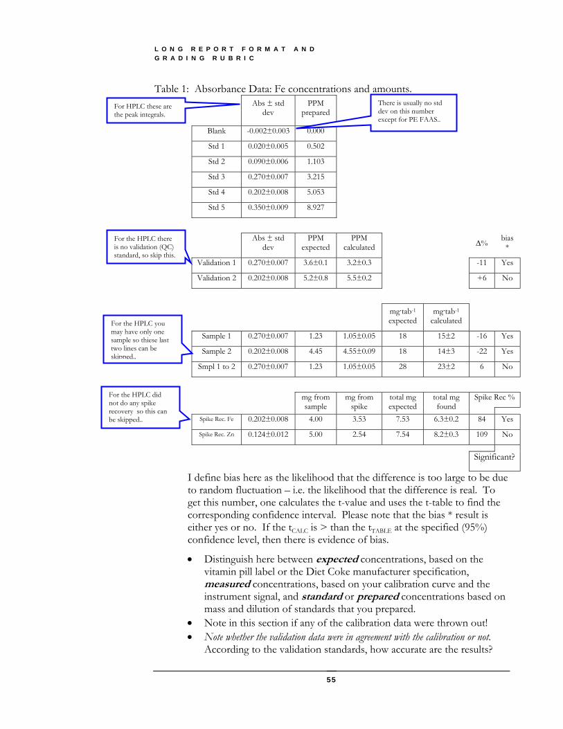
Table 1: Absorbance Data: Fe concentrations and amounts. Abs ± std

dev PPM

prepared

Blank -0.002±0.003 0.000

Std 1 0.020±0.005 0.502

Std 2 0.090±0.006 1.103

Std 3 0.270±0.007 3.215

Std 4 0.202±0.008 5.053

Std 5 0.350±0.009 8.927

Abs ± std dev

PPM expected

PPM calculated Δ% bias

*

Validation 1 0.270±0.007 3.6±0.1 3.2±0.3 -11 Yes

Validation 2 0.202±0.008 5.2±0.8 5.5±0.2 +6 No

mg.tab-1

expected mg.tab-1

calculated

Sample 1 0.270±0.007 1.23 1.05±0.05 18 15±2 -16 Yes

Sample 2 0.202±0.008 4.45 4.55±0.09 18 14±3 -22 Yes

Smpl 1 to 2 0.270±0.007 1.23 1.05±0.05 28 23±2 6 No

mg from sample

mg from spike

total mg expected

total mg found

Spike Rec %

Spike Rec. Fe 0.202±0.008 4.00 3.53 7.53 6.3±0.2 84 Yes

Spike Rec. Zn 0.124±0.012 5.00 2.54 7.54 8.2±0.3 109 No

Significant?

I define bias here as the likelihood that the difference is too large to be due to random fluctuation – i.e. the likelihood that the difference is real. To get this number, one calculates the t-value and uses the t-table to find the corresponding confidence interval. Please note that the bias * result is either yes or no. If the tCALC is > than the tTABLE at the specified (95%) confidence level, then there is evidence of bias.

• Distinguish here between expected concentrations, based on the vitamin pill label or the Diet Coke manufacturer specification, measured concentrations, based on your calibration curve and the instrument signal, and standard or prepared concentrations based on mass and dilution of standards that you prepared.

• Note in this section if any of the calibration data were thrown out! • Note whether the validation data were in agreement with the calibration or not.

According to the validation standards, how accurate are the results?

For the HPLC there is no validation (QC) standard, so skip this.

There is usually no std dev on this number except for PE FAAS..

For the HPLC you may have only one sample so thiese last two lines can be skipped..

For the HPLC did not do any spike recovery so this can be skipped..

For HPLC these are the peak integrals.


56

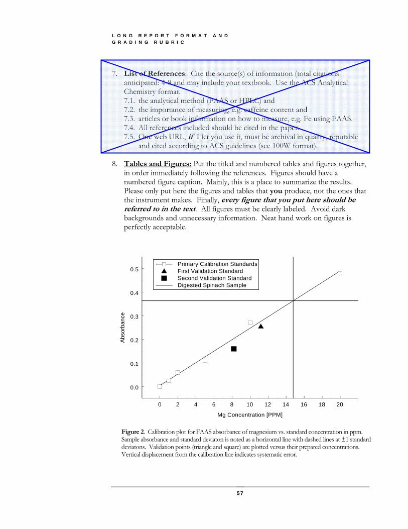
6.6. Make a calibration graph from your analyte absorbance values as

illustrated below. 6.6.1. Preferably on a separate page. 6.6.2. All the points are shown, including:

6.6.2.1. the regression line, 6.6.2.2. validations, 6.6.2.3. the sample absorbance is indicated with a horizontal line

intersecting the calibration line. 6.6.2.4. the uncertainty of the sample absorbance (if known) is

indicated by two parallel lines drawn at the sample absorbance plus and minus the standard deviation in the sample absorbance. Your experimental uncertainty may be too small to do this graphically, but it illustrates nicely the way that the uncertainty in the sample absorbance propagates into an uncertainty in the sample concentration. You may be able to address the question of whether this instrumental method is suitable in terms of detection limit for the given analysis

6.7. [Not required for Analysis Format] Discuss the least-squares (linear

regression) analysis. Note that this implies that you are fitting the data to a model, e.g. A = m*C[PPM] + Sb. Report the best-fit sensitivity, m, and blank signal, Sb and their respective uncertainties. Put the actual regression and propagation of error calculations in the appendix.

6.8. [If validation and sample data are available] Discuss the tests for bias

between validation and expectation, sample and expectation and sample-sample. This is a simple conversation.

6.9. Do not forget to list the final results of the analysis here. This means the

amount of the analyte that is in a meaningful amount (e.g. a serving) of the original sample, e.g. 4 grams of spinach or 12 ounces of diet coke. Compare this value to what is expected for this product.

6.10. Make it clear that you understand the results. Discuss the relative

value of the validation versus random errors. Do sample-to-sample variations swamp the calculated standard deviations and if so, what does this mean?

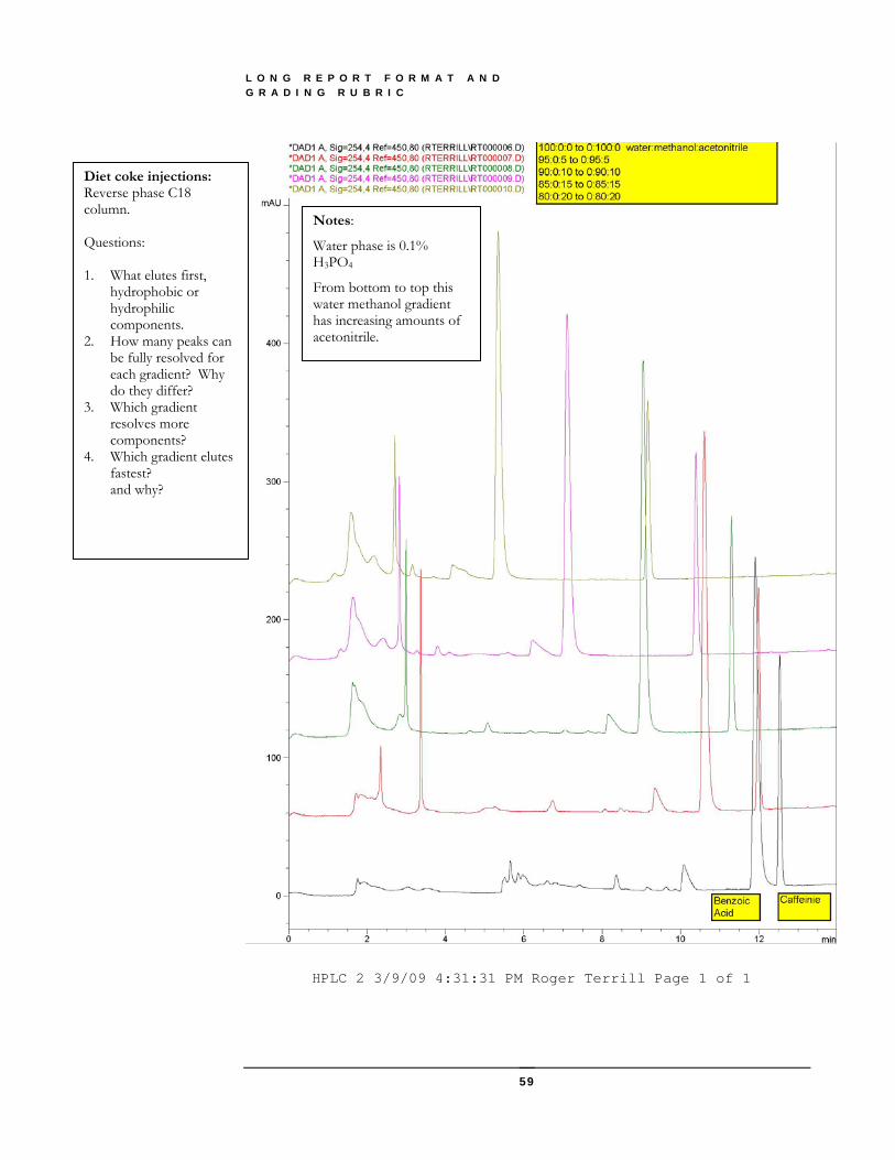
6.11. For the HPLC report, discuss the gradient separations as indicated

on the printout.

6.12. References: List the references here that correspond to the numbered citations in the text. Just like you were taught in 100W. References must be archival sources, that is, no web URL’s without my explicit permission. NIST may be the only exception I make.


57

7. List of References: Cite the source(s) of information (total citations

anticipated: 4-8 and may include your textbook. Use the ACS Analytical Chemistry format. 7.1. the analytical method (FAAS or HPLC) and 7.2. the importance of measuring, e.g. caffeine content and 7.3. articles or book information on how to measure, e.g. Fe using FAAS. 7.4. All references included should be cited in the paper. 7.5. One web URL, if I let you use it, must be archival in quality, reputable

and cited according to ACS guidelines (see 100W format). 8. Tables and Figures: Put the titled and numbered tables and figures together,

in order immediately following the references. Figures should have a numbered figure caption. Mainly, this is a place to summarize the results. Please only put here the figures and tables that you produce, not the ones that the instrument makes. Finally, every figure that you put here should be referred to in the text. All figures must be clearly labeled. Avoid dark backgrounds and unnecessary information. Neat hand work on figures is perfectly acceptable.

0 2 4 6 8 10 12 14 16 18 20

Mg Concentration [PPM]

0.0

0.1

0.2

0.3

0.4

0.5

Abso

rban

ce

Primary Calibration StandardsFirst Validation StandardSecond Validation StandardDigested Spinach Sample

Figure 2. Calibration plot for FAAS absorbance of magnesium vs. standard concentration in ppm. Sample absorbance and standard deviaton is noted as a horizontal line with dashed lines at ±1 standard deviatons. Validation points (triangle and square) are plotted versus their prepared concentrations. Vertical displacement from the calibration line indicates systematic error.


58

9. Appendix: Put your calculations here. Neat handwork is fine – but I expect to see samples of all the important calculations that you performed. If you used a computer program (e.g. Microsoft Excel®) please print out a report from the program illustrating the results. I do not expect anyone to do the linear regression by hand! Some students like to use MathCad for this, and it is extremely efficient and transparent for this goal.


59

HPLC 2 3/9/09 4:31:31 PM Roger Terrill Page 1 of 1

Notes:

Water phase is 0.1% H3PO4

From bottom to top this water methanol gradient has increasing amounts of acetonitrile.

Diet coke injections: Reverse phase C18 column. Questions: 1. What elutes first,

hydrophobic or hydrophilic components.

2. How many peaks can be fully resolved for each gradient? Why do they differ?

3. Which gradient resolves more components?

4. Which gradient elutes fastest? and why?

G U I D E T O D A T A A N A L Y S I S

60

Guide to Data Analysis: Long and Analysis Format Reports

A major learning objective for this course is the successful and complete analysis of the data from a linear regression analysis. Our graduates consistently report that this skill, working with Excel in this way, was one of the most important things they learned in 155.

Math

9


61

T H E O V E R A L L F L O W O F Y O U R D A T A A N A L Y S I S W I L L B E T H I S :

1. Plot calibration data in Excel or equivalent.

2. Get regression coefficients (slope and intercept of best fit calibration line). Use

spreadsheet to calculate sums, products etc.

3. Calculate the concentrations of your samples and validations.

4. Calculate the standard deviation estimates of your sample and validation concentrations

(details on that in the supplement “Guidance for Using Excel for Regression Analysis in

Report” – uses Skoog appendix a1C, equation a1-37)

5. Use the sample preparation procedure to calculate the amount (in mg) of analyte in your

sample specimen (vitamin tablet or can of coke, details below).

6. Use the error propagation rules to calculate the standard deviations in mg of analyte in

your sample specimen. See Skoog appendix a1B-5.

7. Use the t-test to evaluate the difference between the expected and measured values. See

guidance below.

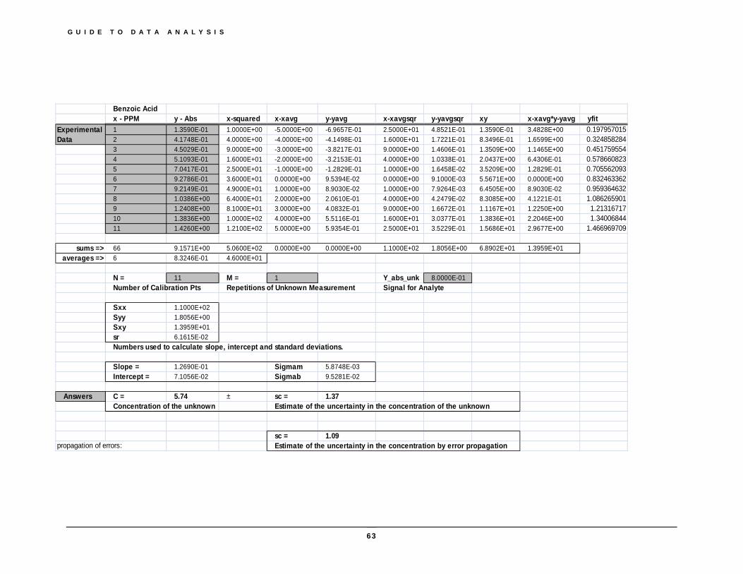
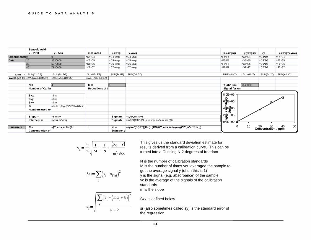
The following two pages contain printouts of a calibration curve analysis of the HPLC data from a previous lab. The first page displays the numbers, with experimental data in the gray, shaded area. The second page displays the formulae used to calculate the results. Please use this as an example for the creation of a spreadsheet of your own that you will use to analyze the data in your homework sets (as applicable) as well as your two principle lab reports (HPLC and FAAS) analyses. While Excel will perform linear regression and give you the slope and intercept of the line that best fits your data, it will not give you the errors in the coefficients or sufficient data to do an error analysis of a predicted value that you may derive from using the (linear) calibration curve coefficients. The worksheet uses formulae identical to those found in Skoog Appendix A, and these have been shown to work – with one exception! In the 5th edition, there is a mistake in In Appendix 1, A-19:

The least squares slope of a line is incorrectly given as: m = Sxx / Syy This should read: m = Sxy / Sxx


62

N O T E S O N U S I N G E X C E L :

If you want a cell to contain a formula – that is, the result of a calculation based on other cell’s data – then you must enter the formula starting with ‘=’. It you use the Excel toolbar button, for example, to enter a sum (Σ), then the ‘=’ will be entered for you. If the result that you get is important, and will be used in other calculations, you can name that cell, and it’s result. So, in doing this spreadsheet, I named the calculations the same way that Skoog did in appendix A, with names like SXX and SXY etc. That way, I can enter the name of the cell in later calculations, rather than the cell itself (e.g. C4). The advantage of this is twofold. First, the formulas are much clearer if they contain names as opposed to cell addresses like C4. Second, if the SXY cell moves (for example if you insert a row to add data), then C4 changes, but SXY does not! So your formula does not need to be changed if you reference a named cell. To name a cell, simply single-click on the cell (so that the focus is on the cell, not to be editing in the cell, the result of a double-click on the cell). Then click on Insert Name Define and give the cell a name (like ‘Sxy’ or ‘m’ or ‘slope’ or ‘answer’ or ‘concentration’ or whatever you prefer).


63

Benzoic Acidx - PPM y - Abs x-squared x-xavg y-yavg x-xavgsqr y-yavgsqr xy x-xavg*y-yavg yfit

Experimental 1 1.3590E-01 1.0000E+00 -5.0000E+00 -6.9657E-01 2.5000E+01 4.8521E-01 1.3590E-01 3.4828E+00 0.197957015Data 2 4.1748E-01 4.0000E+00 -4.0000E+00 -4.1498E-01 1.6000E+01 1.7221E-01 8.3496E-01 1.6599E+00 0.324858284

3 4.5029E-01 9.0000E+00 -3.0000E+00 -3.8217E-01 9.0000E+00 1.4606E-01 1.3509E+00 1.1465E+00 0.4517595544 5.1093E-01 1.6000E+01 -2.0000E+00 -3.2153E-01 4.0000E+00 1.0338E-01 2.0437E+00 6.4306E-01 0.5786608235 7.0417E-01 2.5000E+01 -1.0000E+00 -1.2829E-01 1.0000E+00 1.6458E-02 3.5209E+00 1.2829E-01 0.7055620936 9.2786E-01 3.6000E+01 0.0000E+00 9.5394E-02 0.0000E+00 9.1000E-03 5.5671E+00 0.0000E+00 0.8324633627 9.2149E-01 4.9000E+01 1.0000E+00 8.9030E-02 1.0000E+00 7.9264E-03 6.4505E+00 8.9030E-02 0.9593646328 1.0386E+00 6.4000E+01 2.0000E+00 2.0610E-01 4.0000E+00 4.2479E-02 8.3085E+00 4.1221E-01 1.0862659019 1.2408E+00 8.1000E+01 3.0000E+00 4.0832E-01 9.0000E+00 1.6672E-01 1.1167E+01 1.2250E+00 1.2131671710 1.3836E+00 1.0000E+02 4.0000E+00 5.5116E-01 1.6000E+01 3.0377E-01 1.3836E+01 2.2046E+00 1.3400684411 1.4260E+00 1.2100E+02 5.0000E+00 5.9354E-01 2.5000E+01 3.5229E-01 1.5686E+01 2.9677E+00 1.466969709

sums => 66 9.1571E+00 5.0600E+02 0.0000E+00 0.0000E+00 1.1000E+02 1.8056E+00 6.8902E+01 1.3959E+01averages => 6 8.3246E-01 4.6000E+01

N = 11 M = 1 Y_abs_unk 8.0000E-01Number of Calibration Pts Repetitions of Unknown Measurement Signal for Analyte

Sxx 1.1000E+02Syy 1.8056E+00Sxy 1.3959E+01sr 6.1615E-02Numbers used to calculate slope, intercept and standard deviations.

Slope = 1.2690E-01 Sigmam 5.8748E-03Intercept = 7.1056E-02 Sigmab 9.5281E-02

Answers C = 5.74 ± sc = 1.37Concentration of the unknown Estimate of the uncertainty in the concentration of the unknown

sc = 1.09propagation of errors: Estimate of the uncertainty in the concentration by error propagation


64

Benzoic Acidx - PPM y - Abs x-squared x-xavg y-yavg x-xavgsqr y-yavgsqr xy x-xavg*y-yavg

Experimental0 0 =C4*C4 =C4-xavg =D4-yavg =F4*F4 =G4*G4 =C4*D4 =F4*G4Data 20 3630000 =C5*C5 =C5-xavg =D5-yavg =F5*F5 =G5*G5 =C5*D5 =F5*G5

30 5770000 =C6*C6 =C6-xavg =D6-yavg =F6*F6 =G6*G6 =C6*D6 =F6*G640 7130000 =C7*C7 =C7-xavg =D7-yavg =F7*F7 =G7*G7 =C7*D7 =F7*G7

sums => =SUM(C4:C7) =SUM(D4:D7) =SUM(E4:E7) =SUM(F4:F7) =SUM(G4:G7) =SUM(H4:H7) =SUM(I4:I7) =SUM(J4:J7) =SUM(K4:K7)averages => =AVERAGE(C4:C7) =AVERAGE(D4:D7) =AVERAGE(E4:E7)

N = 4 M = 1 Y_abs_unk 1440000Number of Calibr Repetitions of U Signal for Ana

Sxx =SxxSyy =SyySxy =Sxysr =SQRT((Syy-(m*m*Sxx))/N-2)Numbers used to

Slope = =Sxy/Sxx Sigmam =sy/SQRT(Sxx)Intercept = =yavg-m*xavg Sigmab =sy/(SQRT(1/(N-(sumx*sumx/sumxsqr))))

Answers C = =(Y_abs_unk-b)/m ± sc = =sy/m*(SQRT((1/m)+(1/N)+(Y_abs_unk-yavg)^2/(m*m*Sxx)))Concentration of Estimate of

0.0E+00

2.0E+06

4.0E+06

6.0E+06

8.0E+06

0 10 20 30 40 50

Sign

al /

Arb

itrar

y U

nits

Concentration / ppm

This gives us the standard deviation estimate for results derived from a calibration curve. This can be turned into a CI using N-2 degrees of freedom.

N is the number of calibration standardsM is the number of times you averaged the sample to get the average signal y (often this is 1)y is the signal (e.g. absorbance) of the sampleyc is the average of the signals of the calibration standardsm is the slope

Sxx is defined below

sr (also sometimes called sy) is the standard error of the regression.

scsrm

1M

1N

+yc y−( )m2 Sxx⋅

+⋅

Sxx

i

xi xavg−( )2∑

sri

yi m xi⋅ b+( )−⎡⎣ ⎤⎦2∑

N 2−


65

C O M P A R I N G Y O U R A N S W E R W I T H W H A T Y O U T H I N K T H E A N S W E R S H O U L D B E .

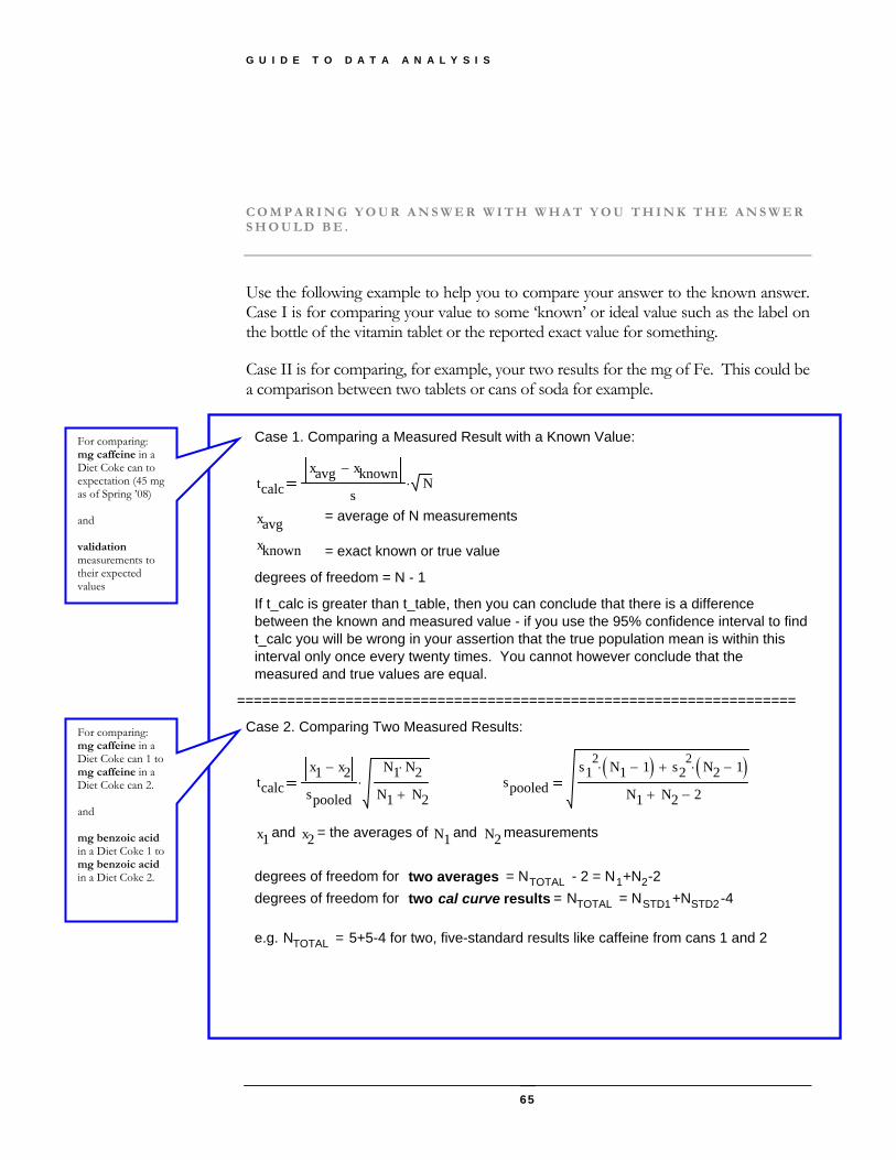
Use the following example to help you to compare your answer to the known answer. Case I is for comparing your value to some ‘known’ or ideal value such as the label on the bottle of the vitamin tablet or the reported exact value for something.

Case II is for comparing, for example, your two results for the mg of Fe. This could be a comparison between two tablets or cans of soda for example.

Case 1. Comparing a Measured Result with a Known Value:

tcalcxavg xknown−

sN⋅

xavg = average of N measurements

xknown = exact known or true value

degrees of freedom = N - 1

If t_calc is greater than t_table, then you can conclude that there is a difference between the known and measured value - if you use the 95% confidence interval to find t_calc you will be wrong in your assertion that the true population mean is within this interval only once every twenty times. You cannot however conclude that the measured and true values are equal.

===================================================================

Case 2. Comparing Two Measured Results:

tcalcx1 x2−

spooled

N1 N2⋅

N1 N2+⋅ spooled

s12 N1 1−( )⋅ s2

2 N2 1−( )⋅+

N1 N2+ 2−

x1 and x2 = the averages of N1 and N2 measurements

degrees of freedom for two averages = NTOTAL - 2 = N1+N2-2 degrees of freedom for two cal curve results = NTOTAL = NSTD1+NSTD2-4

e.g. NTOTAL = 5+5-4 for two, five-standard results like caffeine from cans 1 and 2

For comparing: mg caffeine in a Diet Coke can to expectation (45 mg as of Spring ’08) and validation measurements to their expected values

For comparing: mg caffeine in a Diet Coke can 1 to mg caffeine in a Diet Coke can 2. and mg benzoic acid in a Diet Coke 1 to mg benzoic acid in a Diet Coke 2.


66

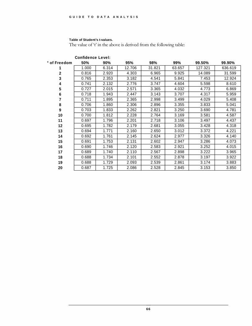
Table of Student’s t-values. The value of ‘t’ in the above is derived from the following table:

Confidence Level:° of Freedom 50% 90% 95% 98% 99% 99.50% 99.90%

1 1.000 6.314 12.706 31.821 63.657 127.321 636.6192 0.816 2.920 4.303 6.965 9.925 14.089 31.5993 0.765 2.353 3.182 4.541 5.841 7.453 12.9244 0.741 2.132 2.776 3.747 4.604 5.598 8.6105 0.727 2.015 2.571 3.365 4.032 4.773 6.8696 0.718 1.943 2.447 3.143 3.707 4.317 5.9597 0.711 1.895 2.365 2.998 3.499 4.029 5.4088 0.706 1.860 2.306 2.896 3.355 3.833 5.0419 0.703 1.833 2.262 2.821 3.250 3.690 4.78110 0.700 1.812 2.228 2.764 3.169 3.581 4.58711 0.697 1.796 2.201 2.718 3.106 3.497 4.43712 0.695 1.782 2.179 2.681 3.055 3.428 4.31813 0.694 1.771 2.160 2.650 3.012 3.372 4.22114 0.692 1.761 2.145 2.624 2.977 3.326 4.14015 0.691 1.753 2.131 2.602 2.947 3.286 4.07316 0.690 1.746 2.120 2.583 2.921 3.252 4.01517 0.689 1.740 2.110 2.567 2.898 3.222 3.96518 0.688 1.734 2.101 2.552 2.878 3.197 3.92219 0.688 1.729 2.093 2.539 2.861 3.174 3.88320 0.687 1.725 2.086 2.528 2.845 3.153 3.850


67

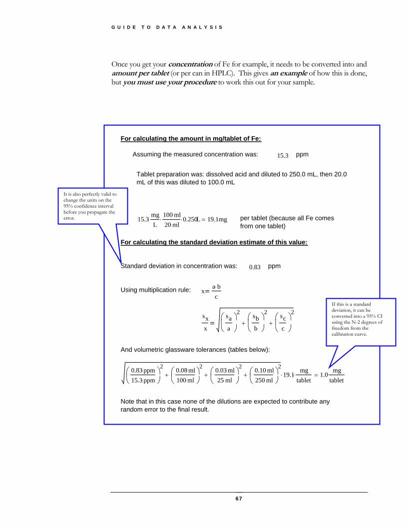
Once you get your concentration of Fe for example, it needs to be converted into and amount per tablet (or per can in HPLC). This gives an example of how this is done, but you must use your procedure to work this out for your sample.

Note that in this case none of the dilutions are expected to contribute any random error to the final result.

0.83 ppm⋅

15.3 ppm⋅⎛⎜⎝

⎞⎟⎠

2 0.08 ml⋅

100 ml⋅⎛⎜⎝

⎞⎟⎠

2+

0.03 ml⋅

25 ml⋅⎛⎜⎝

⎞⎟⎠

2+

0.10 ml⋅

250 ml⋅⎛⎜⎝

⎞⎟⎠

2+ 19.1⋅

mgtablet⋅ 1.0

mgtablet

=

And volumetric glassware tolerances (tables below):

sxx

saa

⎛⎜⎝

⎞⎟⎠

2 sbb

⎛⎜⎝

⎞⎟⎠

2

+scc

⎛⎜⎝

⎞⎟⎠

2

+

xa b⋅c

Using multiplication rule:

ppm0.83Standard deviation in concentration was:

For calculating the standard deviation estimate of this value:

per tablet (because all Fe comes from one tablet)

15.3mgL

⋅100 ml⋅

20 ml⋅⋅ 0.250⋅ L 19.1mg=

Tablet preparation was: dissolved acid and diluted to 250.0 mL, then 20.0 mL of this was diluted to 100.0 mL

ppm15.3Assuming the measured concentration was:

For calculating the amount in mg/tablet of Fe:

It is also perfectly valid to change the units on the 95% confidence interval before you propagate the error.

If this is a standard deviation, it can be converted into a 95% CI using the N-2 degrees of freedom from the calibration curve.


68

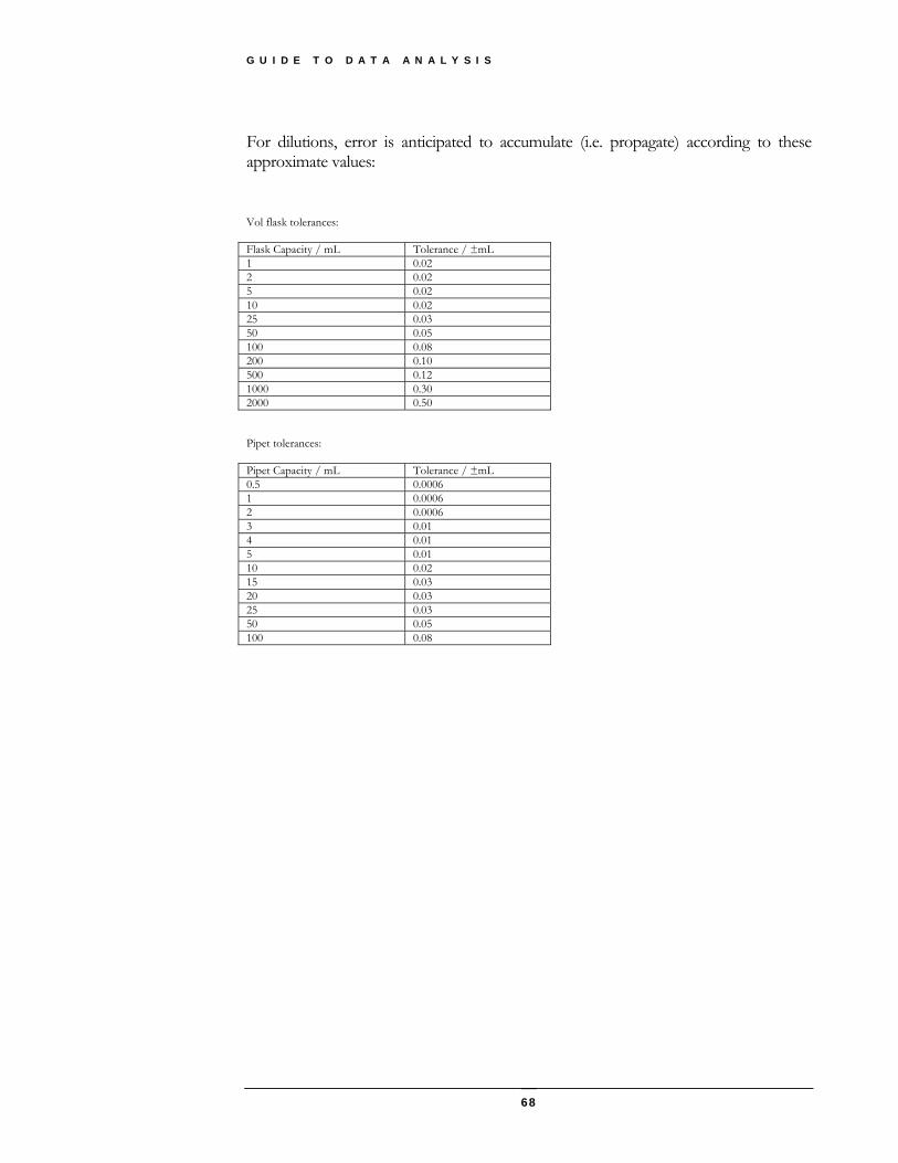
For dilutions, error is anticipated to accumulate (i.e. propagate) according to these approximate values:

Vol flask tolerances: Flask Capacity / mL Tolerance / ±mL 1 0.02 2 0.02 5 0.02 10 0.02 25 0.03 50 0.05 100 0.08 200 0.10 500 0.12 1000 0.30 2000 0.50 Pipet tolerances: Pipet Capacity / mL Tolerance / ±mL 0.5 0.0006 1 0.0006 2 0.0006 3 0.01 4 0.01 5 0.01 10 0.02 15 0.03 20 0.03 25 0.03 50 0.05 100 0.08


69

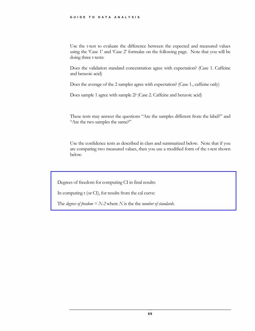
Use the t-test to evaluate the difference between the expected and measured values using the ‘Case 1’ and ‘Case 2’ formulas on the following page. Note that you will be doing three t-tests:

Does the validation standard concentration agree with expectation? (Case 1. Caffeine and benzoic acid)

Does the average of the 2 samples agree with expectation? (Case 1., caffeine only)

Does sample 1 agree with sample 2? (Case 2. Caffeine and benzoic acid)

These tests may answer the questions “Are the samples different from the label?” and “Are the two samples the same?”

Use the confidence tests as described in class and summarized below. Note that if you are comparing two measured values, then you use a modified form of the t-test shown below.

Degrees of freedom for computing CI in final results:

In computing t (or CI), for results from the cal curve:

The degrees of freedom = N-2 where N is the the number of standards.


70

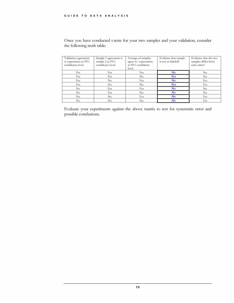
Once you have conducted t-tests for your two samples and your validation, consider the following truth table:

Validation agreement w expectation at 95% confidence level.

Sample 1 agreement w sample 2 at 95% confidence level.

Average of samples agree w/ expectation at 95% confidence level.

Evidence that sample is not as labeled?

Evidence that the two samples differ from each other?

Yes Yes Yes No No Yes Yes No Yes No Yes No Yes No Yes Yes No No Yes Yes No Yes Yes No No No Yes No No No No No Yes No Yes No No No No Yes

Evaluate your experiments against the above matrix to test for systematic error and possible conclusions.

Documents

LONG REPORT FORMAT AND Long and GRADING RUBRIC …