Long-period, long-duration seismic events during hydraulic stimulationof shale and tight-gas reservoirs — Part 1: Waveform characteristics

Indrajit Das1 and Mark D. Zoback1

ABSTRACT

Long-period long-duration (LPLD) seismic events arerelatively low-amplitude signals that have been observed dur-ing hydraulic fracturing in several shale-gas and tight-gas res-ervoirs. These events are similar in appearance to tectonictremor sequences observed in subduction zones and transformfault boundaries. LPLD events are predominantly composed ofS-waves, but weaker P-waves have also been identified. Insome cases, microearthquakes are observed during the events.Based on the similarity with tectonic tremors and our obser-vations of several impulsive S-wave arrivals within the LPLDevents, we interpret the LPLD events as resulting from thesuperposition of slow shear-slip events on relatively largefaults. Most large LPLD waveforms appear to start as a

relatively slower, low-amplitude precursor, lacking clear im-pulsive arrivals. We estimate the energy carried by the largerLPLD events to be ∼1000 times greater than a ∼MW − 2 mi-croseismic event that is typical of the events that occur duringhydraulic stimulation. Over the course of the entire stimulationactivity of five wells in the Barnett formation (each hydrauli-cally fractured ten times), the LPLD events were found tocumulatively release over an order of magnitude higher energythan microearthquakes. The large size of these LPLD events,compared to microearthquakes, suggests that they representslip on relatively large faults during stimulation of theseextremely low-permeability reservoirs. Moreover, they implythat the accompanying slow slip on faults, probably mostlyundetected, is a significant deformation process during multi-stage hydraulic fracturing.

INTRODUCTION

Although horizontal drilling and multistage hydraulic fracturingare successfully used to stimulate production from shale-gas, tight-gas, and tight-oil reservoirs, the principal deformation mechanismsresponsible for the stimulation of production from these extremelylow-permeability formations are still poorly understood. It has beenwell documented that, during multistage horizontal fracturing, a“cloud” of microseismic events surrounding the hydraulic fracturesindicate the occurrence of shear slip on preexisting fractures andfaults distributed around the induced hydraulic fractures (Rutledgeand Phillips, 2003; Warpinski et al., 2004). However, the correlationbetween the cloud of microseismic event and the stimulated rockvolume is still questioned (Sicking et al., 2013). In a case in whichthe microseismic cloud was fairly planar, Moos et al. (2011) showedthat the number of microseismic events did not correlate with pro-duction from successive hydraulic fracturing stages.

The motivation of this paper is to investigate the other sources ofdeformation that occur in these unconventional reservoirs duringhydraulic stimulation. In a preliminary study of seismic waveformsrecorded at depth during multistage hydraulic fracturing in five par-allel wells in the Barnett shale, Das and Zoback (2011) documentedthe occurrence of long-period long-duration (LPLD) seismic events.The observed LPLD events have similarities to seismic eventsknown as tectonic tremors observed in subduction zones and trans-form boundaries (Southwest Japan, Cascadia, San Andreas Fault;Obara, 2002; Shelly et al., 2006; Nadeau and Guilheim, 2009). Sev-eral authors (Rogers and Dragert, 2003; Obara et al., 2004; Hiroseand Obara, 2010; Bartlow et al., 2011) have shown that tremor ac-companies slow shear-slip events, in some cases independently seengeodetically, localized in the transition zone between the locked andsliding portion of major plate-boundary faults such as subductionthrusts and the San Andreas fault. Das and Zoback (2011) suggestedthat the LPLD signals observed provide evidence of similar

Manuscript received by the Editor 24 April 2013; revised manuscript received 2 July 2013; published online 21 October 2013.1Stanford University, Geophysics Department, Palo Alto, California, USA. E-mail: idas@stanford.edu; zoback@stanford.edu.© 2013 Society of Exploration Geophysicists. All rights reserved.

KS107

GEOPHYSICS, VOL. 78, NO. 6 (NOVEMBER-DECEMBER 2013); P. KS107–KS118, 13 FIGS.10.1190/GEO2013-0164.1

Dow

nloa

ded

10/2

8/13

to 9

8.19

8.23

.207

. Red

istr

ibut

ion

subj

ect t

o SE

G li

cens

e or

cop

yrig

ht; s

ee T

erm

s of

Use

at h

ttp://

libra

ry.s

eg.o

rg/

deformation mechanisms happening during multistage hydraulicstimulation of gas fields. Zoback et al. (2012) expanded upon thisinterpretation, and provides reasons why slow slip on preexistingfaults appears to be an important deformation process during multi-stage hydraulic fracturing and could potentially contribute appreci-ably to reservoir production.Geiser et al. (2012) observe seismic signals that differ from con-

ventional microearthquakes during hydraulic stimulation. By stack-ing the energy from these signals over periods of minutes to hours,they have identified linear sources of low-frequency energy, whichthey have interpreted to be natural fracture pathways.Eaton et al. (2013) undertook a study in the Canadian Montney

gas reservoir looking at low-frequency signals generated during hy-draulic fracturing and were able to observe signals which resembledLPLD events, although they were not so numerous or energetic asthose Das and Zoback (2011) identified in the Barnett. LPLD eventswere also observed in a multistage hydraulic fracture stimula-tion project in the Cardium formation in west central Alberta(A. St-Onge, personal communication, 2013).In this paper, we discuss the characteristics of the LPLD events

recorded during passive seismic monitoring of multistage hydraulicfracturing projects in four different case studies. We look in detail atLPLD events in two of these data sets from the Barnett Shale inTexas and illustrate their occurrence in a tight-gas sand reservoirin Canada and a shale-gas reservoir in Canada. In a companionpaper (Das and Zoback, 2013), we explore in detail where, when,and why the LPLD events occur in a reservoir during hydraulicstimulation, and the physical processes responsible for theiroccurrence.

DATA SETS ANALYZED

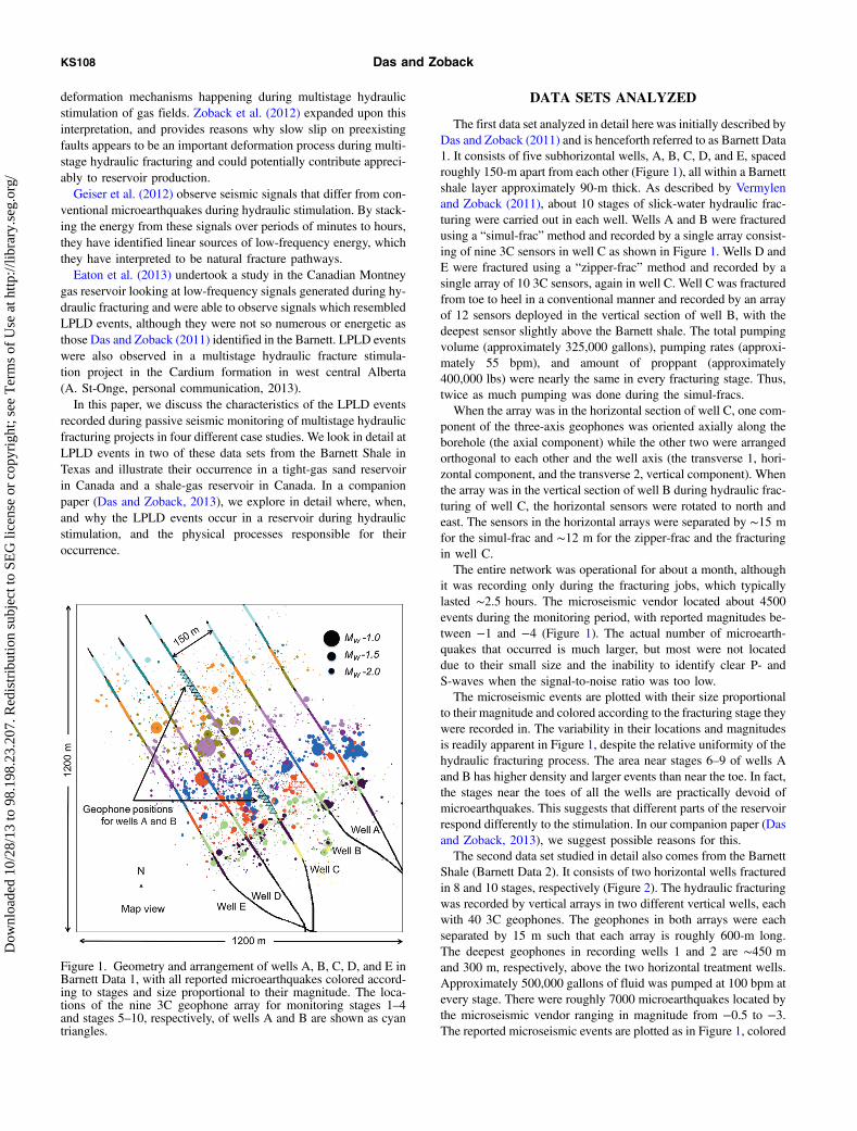
The first data set analyzed in detail here was initially described byDas and Zoback (2011) and is henceforth referred to as Barnett Data1. It consists of five subhorizontal wells, A, B, C, D, and E, spacedroughly 150-m apart from each other (Figure 1), all within a Barnettshale layer approximately 90-m thick. As described by Vermylenand Zoback (2011), about 10 stages of slick-water hydraulic frac-turing were carried out in each well. Wells A and B were fracturedusing a “simul-frac” method and recorded by a single array consist-ing of nine 3C sensors in well C as shown in Figure 1. Wells D andE were fractured using a “zipper-frac” method and recorded by asingle array of 10 3C sensors, again in well C. Well C was fracturedfrom toe to heel in a conventional manner and recorded by an arrayof 12 sensors deployed in the vertical section of well B, with thedeepest sensor slightly above the Barnett shale. The total pumpingvolume (approximately 325,000 gallons), pumping rates (approxi-mately 55 bpm), and amount of proppant (approximately400,000 lbs) were nearly the same in every fracturing stage. Thus,twice as much pumping was done during the simul-fracs.When the array was in the horizontal section of well C, one com-

ponent of the three-axis geophones was oriented axially along theborehole (the axial component) while the other two were arrangedorthogonal to each other and the well axis (the transverse 1, hori-zontal component, and the transverse 2, vertical component). Whenthe array was in the vertical section of well B during hydraulic frac-turing of well C, the horizontal sensors were rotated to north andeast. The sensors in the horizontal arrays were separated by ∼15 m

for the simul-frac and ∼12 m for the zipper-frac and the fracturingin well C.The entire network was operational for about a month, although

it was recording only during the fracturing jobs, which typicallylasted ∼2.5 hours. The microseismic vendor located about 4500events during the monitoring period, with reported magnitudes be-tween −1 and −4 (Figure 1). The actual number of microearth-quakes that occurred is much larger, but most were not locateddue to their small size and the inability to identify clear P- andS-waves when the signal-to-noise ratio was too low.The microseismic events are plotted with their size proportional

to their magnitude and colored according to the fracturing stage theywere recorded in. The variability in their locations and magnitudesis readily apparent in Figure 1, despite the relative uniformity of thehydraulic fracturing process. The area near stages 6–9 of wells Aand B has higher density and larger events than near the toe. In fact,the stages near the toes of all the wells are practically devoid ofmicroearthquakes. This suggests that different parts of the reservoirrespond differently to the stimulation. In our companion paper (Dasand Zoback, 2013), we suggest possible reasons for this.The second data set studied in detail also comes from the Barnett

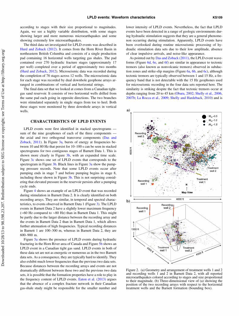
Shale (Barnett Data 2). It consists of two horizontal wells fracturedin 8 and 10 stages, respectively (Figure 2). The hydraulic fracturingwas recorded by vertical arrays in two different vertical wells, eachwith 40 3C geophones. The geophones in both arrays were eachseparated by 15 m such that each array is roughly 600-m long.The deepest geophones in recording wells 1 and 2 are ∼450 m

and 300 m, respectively, above the two horizontal treatment wells.Approximately 500,000 gallons of fluid was pumped at 100 bpm atevery stage. There were roughly 7000 microearthquakes located bythe microseismic vendor ranging in magnitude from −0.5 to −3.The reported microseismic events are plotted as in Figure 1, colored

Figure 1. Geometry and arrangement of wells A, B, C, D, and E inBarnett Data 1, with all reported microearthquakes colored accord-ing to stages and size proportional to their magnitude. The loca-tions of the nine 3C geophone array for monitoring stages 1–4and stages 5–10, respectively, of wells A and B are shown as cyantriangles.

KS108 Das and Zoback

Dow

nloa

ded

10/2

8/13

to 9

8.19

8.23

.207

. Red

istr

ibut

ion

subj

ect t

o SE

G li

cens

e or

cop

yrig

ht; s

ee T

erm

s of

Use

at h

ttp://

libra

ry.s

eg.o

rg/

according to stages with their size proportional to magnitudes.Again, we see a highly variable distribution, with some stagesshowing larger and more numerous microearthquakes and someshowing extremely few microearthquakes.The third data set investigated for LPLD events was described in

Hurd and Zoback (2012). It comes from the Horn River Basin innortheastern British Columbia and consists of a single productionpad containing 16 horizontal wells targeting gas shales. The padcontained over 270 hydraulic fracture stages (approximately 17per well) completed over a period of approximately two months(Hurd and Zoback, 2012). Microseismic data was recorded duringthe completion of 78 stages across 12 wells. The microseismic datafor each stage was recorded by dual downhole geophone arrays ar-ranged in combinations of vertical and horizontal strings.The final data set that we looked at comes from a Canadian tight-

gas sand reservoir. It consists of two horizontal wells drilled fromthe same pad each going in opposite directions. The two brancheswere stimulated separately in single stages from toe to heel. Boththese stages were monitored by three downhole arrays in verticalwells.

CHARACTERISTICS OF LPLD EVENTS

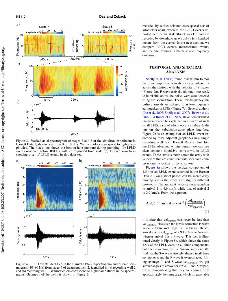
LPLD events were first identified in stacked spectrograms —sum of the nine geophones of each of the three components —the axial and two orthogonal transverse components (Das andZoback, 2011). In Figure 3a, bursts of energy at frequencies be-tween 10 and 80 Hz that persist for 10–100 s can be seen in stackedspectrograms for two contiguous stages of Barnett Data 1. This isshown more clearly in Figure 3b, with an expanded time scale.Figure 3c shows one set of LPLD events that corresponds to thespectrogram in Figure 3b. Black lines in Figure 3a show the pump-ing pressure records. Note that some LPLD events occur afterpumping ends in stage 7 and before pumping begins in stage 8,including those shown in Figure 3b. This is not surprising consid-ering that elevated pressure in the reservoir persists after a pumpingcycle ends.Figure 4 shows an example of an LPLD event that was recorded

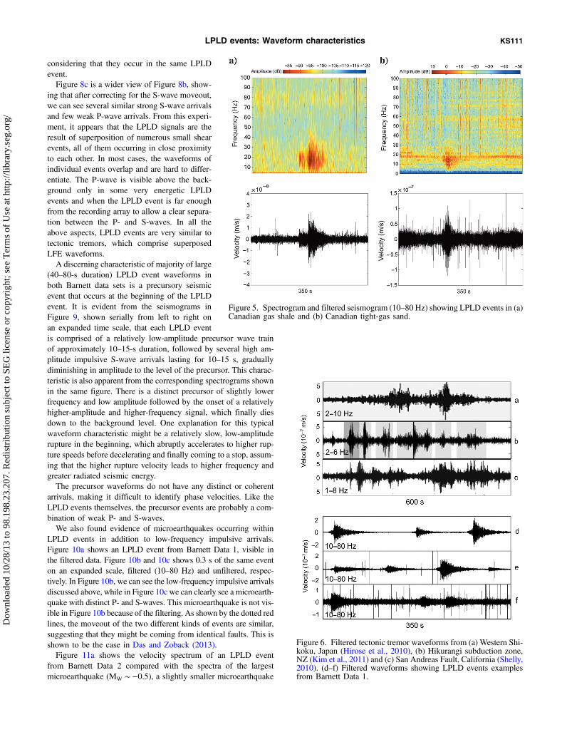
during stimulation in Barnett Data 2. It is clearly identified on bothrecording arrays. They are similar, in temporal and spectral charac-teristics, to events observed in Barnett Data 1 (Figure 3). The LPLDevents in Barnett Data 2 have a slightly lower maximum frequency(∼60 Hz compared to ∼80 Hz) than in Barnett Data 1. This mightbe partly due to the larger distance between the recording array andthe events in Barnett Data 2 than in Barnett Data 1, which allowsfurther attenuation of high frequencies. Typical recording distancesin Barnett 1 are 100–300 m, whereas in Barnett Data 2, they are600–900 m.Figure 5a shows the presence of LPLD events during hydraulic

fracturing in the Horn River area of Canada and Figure 5b shows anLPLD event in a Canadian tight gas sand. LPLD events in both ofthese data set are not as energetic or numerous as in the two Barnettdata sets. As a consequence, they are typically hard to identify. Theyalso exhibit much lower frequencies than the previous two data sets.Because distances between the recording arrays and events are notdramatically different between these two and the previous two datasets, it is possible that the formation properties have a role to play inthe frequency content of LPLD events. Eaton et al. (2013) arguesthat the absence of a complex fracture network in their Canadiangas-shale study might be responsible for the smaller number and

lower intensity of LPLD events. Nevertheless, the fact that LPLDevents have been detected in a range of geologic environments dur-ing hydraulic stimulation suggests that they are a general phenome-non occurring during stimulation. Apparently, LPLD events havebeen overlooked during routine microseismic processing of hy-draulic stimulation data sets due to their low amplitude, absenceof clear impulsive arrivals, and noise-like appearance.As pointed out by Das and Zoback (2011), the LPLD event wave-

forms (Figure 6d, 6e, and 6f) are similar in appearance to tectonictremors (also known as nonvolcanic tremors) observed in subduc-tion zones and strike-slip margins (Figure 6a, 6b, and 6c), althoughtectonic tremors are typically observed between 1 and 15 Hz, a fre-quency band that is not detectable with the 15 Hz geophones usedfor microseismic recording in the four data sets reported here. Thesimilarity is striking despite the fact that tectonic tremors occur atdepths ranging from 20 to 45 km (Obara, 2002; Shelly et al., 2006,2007b; La Rocca et al., 2009; Shelly and Hardeback, 2010) and is

Figure 2. (a) Geometry and arrangement of treatment wells 1 and 2and recording wells 1 and 2 in Barnett Data 2, with all reportedmicroearthquakes colored according to stages and size proportionalto their magnitude. (b) Three-dimensional view of (a) showing theposition of the two recording arrays with respect to the horizontaltreatment wells and the Barnett formation (bounding box).

LPLD events: Waveform characteristics KS109

Dow

nloa

ded

10/2

8/13

to 9

8.19

8.23

.207

. Red

istr

ibut

ion

subj

ect t

o SE

G li

cens

e or

cop

yrig

ht; s

ee T

erm

s of

Use

at h

ttp://

libra

ry.s

eg.o

rg/

recorded by surface seismometers spaced tens ofkilometers apart, whereas the LPLD events re-ported here occur at depths of 2–3 km and arerecorded by downhole arrays only a few hundredmeters from the events. In the next section, wecompare LPLD events, microseismic events,and tectonic tremors in the time and frequencydomains.

TEMPORAL AND SPECTRALANALYSIS

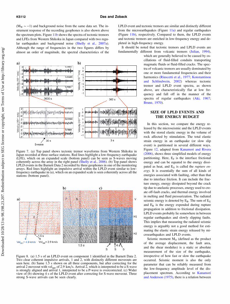
Shelly et al. (2006) found that within tremorthere are impulsive arrivals moving coherentlyacross the stations with the velocity of S-waves(Figure 7a). P-wave arrivals, although too weakto be visible above the noise, were also detectedusing crosscorrelation. These low-frequency im-pulsive arrivals are referred to as low-frequencyearthquakes or LFEs (Figure 7a). Several authors(Ide et al., 2007; Shelly et al., 2007a; Brown et al.,2009; La Rocca et al., 2009) have demonstratedthat tremors can be explained as a swarm of suchsmall LFEs, each of which occurs as shear fault-ing on the subduction-zone plate interface.Figure 7b is an example of an LPLD event re-corded by three adjacent geophones in a singlerecording well from Barnett Data 2. Just likethe LFEs observed within tremor, we can seeclear coherent impulsive arrivals within LPLDevents. These arrivals move across the array withvelocities that are consistent with shear and com-pressional velocities in the reservoir.Figure 8a shows the vertical component of

1.5 s of an LPLD event recorded in the BarnettData 2. Two distinct phases can be seen clearlymoving across the array with slightly differentmoveouts. The apparent velocity correspondingto arrival 1 is 4.9 km∕s while that of arrival 2is 2.9 km∕s. From the equation

Angle of arrival ¼ cos−1�velformation

velapparent

�

(1)

it is clear that velapparent can never be less thanvelformation. However, the lowest formation P-wavevelocity from well logs is 3.6 km∕s. Hence,arrival 2 with velapparent of 2.9 km∕s is an S-wave,whereas arrival 1 is a P-wave. This fact is illus-trated clearly in Figure 8b, which shows the same1.5 s of the LPLD event in all three components,but after correcting for the S-wave moveout. Wefind that the S-wave is strongly aligned in all threecomponents and the P-wave is overcorrected. Us-ing average P- and S-wave velformation, we getsimilar angles of arrival for arrival 1 and 2, respec-tively, demonstrating that they are coming fromapproximately the same area, which is reasonable

Figure 3. Stacked axial spectrogram of stages 7 and 8 of the simulfrac experiment inBarnett Data 1, shown here from 0 to 100 Hz. Warmer colors correspond to higher am-plitudes. The black line shows the bottom-hole pressure during pumping. (b) LPLDevents observed below 100 Hz with an expanded time scale. (c) Filtered waveformshowing a set of LPLD events in this data set.

Figure 4. LPLD events identified in the Barnett Data 2. Spectrogram and filtered seis-mogram (10–80 Hz) from stage 4 of treatment well 2, identified in (a) recording well 2and (b) recording well 1. Warmer colors correspond to higher amplitudes in the spectro-grams. Geometry of the wells is shown in Figure 2.

KS110 Das and Zoback

Dow

nloa

ded

10/2

8/13

to 9

8.19

8.23

.207

. Red

istr

ibut

ion

subj

ect t

o SE

G li

cens

e or

cop

yrig

ht; s

ee T

erm

s of

Use

at h

ttp://

libra

ry.s

eg.o

rg/

considering that they occur in the same LPLDevent.Figure 8c is a wider view of Figure 8b, show-

ing that after correcting for the S-wave moveout,we can see several similar strong S-wave arrivalsand few weak P-wave arrivals. From this experi-ment, it appears that the LPLD signals are theresult of superposition of numerous small shearevents, all of them occurring in close proximityto each other. In most cases, the waveforms ofindividual events overlap and are hard to differ-entiate. The P-wave is visible above the back-ground only in some very energetic LPLDevents and when the LPLD event is far enoughfrom the recording array to allow a clear separa-tion between the P- and S-waves. In all theabove aspects, LPLD events are very similar totectonic tremors, which comprise superposedLFE waveforms.A discerning characteristic of majority of large

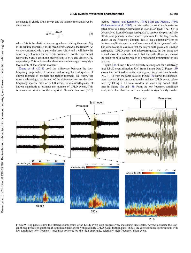
(40–80-s duration) LPLD event waveforms inboth Barnett data sets is a precursory seismicevent that occurs at the beginning of the LPLDevent. It is evident from the seismograms inFigure 9, shown serially from left to right onan expanded time scale, that each LPLD eventis comprised of a relatively low-amplitude precursor wave trainof approximately 10–15-s duration, followed by several high am-plitude impulsive S-wave arrivals lasting for 10–15 s, graduallydiminishing in amplitude to the level of the precursor. This charac-teristic is also apparent from the corresponding spectrograms shownin the same figure. There is a distinct precursor of slightly lowerfrequency and low amplitude followed by the onset of a relativelyhigher-amplitude and higher-frequency signal, which finally diesdown to the background level. One explanation for this typicalwaveform characteristic might be a relatively slow, low-amplituderupture in the beginning, which abruptly accelerates to higher rup-ture speeds before decelerating and finally coming to a stop, assum-ing that the higher rupture velocity leads to higher frequency andgreater radiated seismic energy.The precursor waveforms do not have any distinct or coherent

arrivals, making it difficult to identify phase velocities. Like theLPLD events themselves, the precursor events are probably a com-bination of weak P- and S-waves.We also found evidence of microearthquakes occurring within

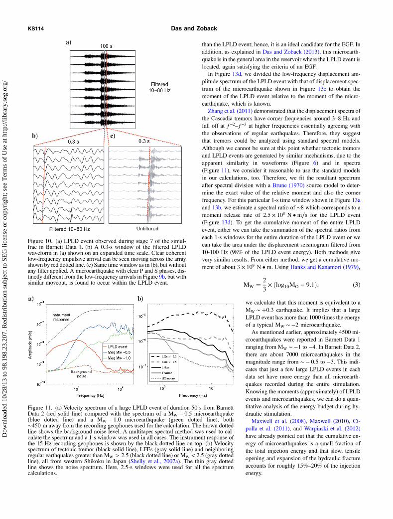
LPLD events in addition to low-frequency impulsive arrivals.Figure 10a shows an LPLD event from Barnett Data 1, visible inthe filtered data. Figure 10b and 10c shows 0.3 s of the same eventon an expanded scale, filtered (10–80 Hz) and unfiltered, respec-tively. In Figure 10b, we can see the low-frequency impulsive arrivalsdiscussed above, while in Figure 10c we can clearly see a microearth-quake with distinct P- and S-waves. This microearthquake is not vis-ible in Figure 10b because of the filtering. As shown by the dotted redlines, the moveout of the two different kinds of events are similar,suggesting that they might be coming from identical faults. This isshown to be the case in Das and Zoback (2013).Figure 11a shows the velocity spectrum of an LPLD event

from Barnett Data 2 compared with the spectra of the largestmicroearthquake (MW ∼ −0.5), a slightly smaller microearthquake

Figure 5. Spectrogram and filtered seismogram (10–80 Hz) showing LPLD events in (a)Canadian gas shale and (b) Canadian tight-gas sand.

Figure 6. Filtered tectonic tremor waveforms from (a) Western Shi-koku, Japan (Hirose et al., 2010), (b) Hikurangi subduction zone,NZ (Kim et al., 2011) and (c) San Andreas Fault, California (Shelly,2010). (d–f) Filtered waveforms showing LPLD events examplesfrom Barnett Data 1.

LPLD events: Waveform characteristics KS111

Dow

nloa

ded

10/2

8/13

to 9

8.19

8.23

.207

. Red

istr

ibut

ion

subj

ect t

o SE

G li

cens

e or

cop

yrig

ht; s

ee T

erm

s of

Use

at h

ttp://

libra

ry.s

eg.o

rg/

(MW ∼ −1) and background noise from the same data set. The in-strument response of the recording geophones is also shown abovethe spectrum plots. Figure 11b shows the spectra of tectonic tremorsand LFEs from Western Shikoku in Japan compared with two regu-lar earthquakes and background noise (Shelly et al., 2007a).Although the range of frequencies in the two figures differs byalmost an order of magnitude, the spectral characteristics of the

LPLD event and tectonic tremors are similar and distinctly differentfrom the microearthquakes (Figure 11a) and regular earthquakes(Figure 11b), respectively. Compared to them, the LPLD eventsand tectonic tremors are enriched in low-frequency energy and de-pleted in high-frequency energy.It should be noted that tectonic tremors and LPLD events are

fundamentally different from volcanic tremors (Julian, 1994),which are generally believed to be caused by os-cillations of fluid-filled conduits transportingmagmatic fluids or fluid-filled cracks. The spec-tra of volcanic tremors are usually dominated byone or more fundamental frequencies and theirharmonics (Riuscetti et al., 1977; Konstantinouand Schlindwein, 2002) whereas tectonictremor and LPLD event spectra, as shownabove, are characteristically flat at low fre-quency and fall off in the manner of thespectra of regular earthquakes (Aki, 1967;Brune, 1970).

SIZE OF LPLD EVENTS ANDTHE ENERGY BUDGET

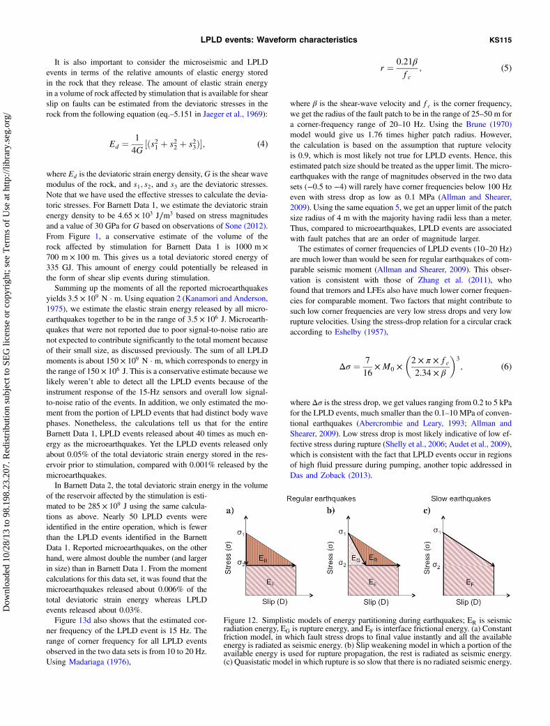
In this section, we compare the energy re-leased by the microseismic and the LPLD eventswith the stored elastic energy in the volume ofrock affected by stimulation. The total elasticstrain energy in an earthquake (or slow slipevent) is partitioned in several different ways.Figure 12, adapted from Kanamori and Rivera(2006), shows three simplified models of energypartitioning. Here, EF is the interface frictionalenergy and can be equated to the energy dissi-pated as heat, and EG is called the rupture en-ergy. It is essentially the sum of all kinds ofenergies associated with faulting, other than thatdue to interface friction. It can include the frac-ture energy, energy dissipated beyond the cracktip due to anelastic processes, energy used to cre-ate off-fault cracks, and thermal energy involvedin melting and fluid pressurization. The radiatedseismic energy is denoted by ER. The sum of EG

and ER is the energy expended during rupturepropagation in addition to frictional dissipation.LPLD events probably lie somewhere in betweenregular earthquakes and slowly slipping faults.This implies that measuring the radiated seismicenergy is arguably not a good method for esti-mating the elastic strain energy released by mi-croearthquakes and LPLD events.Seismic moment MO (defined as the product

of the average displacement, the fault area,and the shear modulus) is a static or absolutemeasurement of the size of the earthquake,irrespective of how fast or slow the earthquakeoccurred. Seismic moment is also the onlyparameter that can be reliably measured fromthe low-frequency amplitude level of the dis-placement spectrum. According to Kanamoriand Anderson (1975), there is a relation between

Figure 7. (a) Top panel shows tectonic tremor waveforms from Western Shikoku inJapan recorded at three surface stations. Red lines highlight a low-frequency earthquake(LFE), which on an expanded scale (bottom panel) can be seen as S-waves movingcoherently across the array in the right panel (Shelly et al., 2006). (b) Top panel showsLPLD events in the Barnett Data 2 recorded by three geophones in one of the monitoringarrays. Red lines highlight an impulsive arrival within the LPLD event similar to low-frequency earthquake in (a), which on an expanded scale is seen coherently across all thestations (bottom panel).

Figure 8. (a) 1.5 s of an LPLD event on component 1 identified in the Barnett Data 2.Two clear coherent impulsive arrivals, 1 and 2, with distinctly different moveouts areseen here. (b) Same 1.5 s shown on all three components, but after correcting for thearrival 2 moveout with velapp of 2.9 km∕s. Arrival 2, which is interpreted to be a S-waveis strongly aligned and arrival 1, interpreted to be a P-wave is overcorrected. (c) Widerview of (b) showing 4 s of the LPLD event after correcting for S-wave moveout. Threestrong S-wave arrivals can be seen clearly.

KS112 Das and Zoback

Dow

nloa

ded

10/2

8/13

to 9

8.19

8.23

.207

. Red

istr

ibut

ion

subj

ect t

o SE

G li

cens

e or

cop

yrig

ht; s

ee T

erm

s of

Use

at h

ttp://

libra

ry.s

eg.o

rg/

the change in elastic strain energy and the seismic moment given bythe equation

ΔW ¼ MOσ̄

μ; (2)

where ΔW is the elastic strain energy released during the event,MO

is the seismic moment, σ̄ is the mean stress, and μ is the rigidity. Aswe are concerned with a particular reservoir, σ̄ and μ will have thesame range of values for the events considered. For the two Barnettreservoirs, σ̄ and μ are in the order of tens of MPa and tens of GPa,respectively. This indicates that the elastic strain energy is roughly athousandth of the seismic moment.Zhang et al. (2011) used the difference between the low-

frequency amplitudes of tremors and of regular earthquakes ofknown moment to estimate the tremor moment. We follow thesame methodology, but instead of the difference, we use the low-frequency spectral ratio of LPLD events to microearthquakes ofknown magnitude to estimate the moment of LPLD events. Thisis somewhat similar to the empirical Green’s function (EGF)

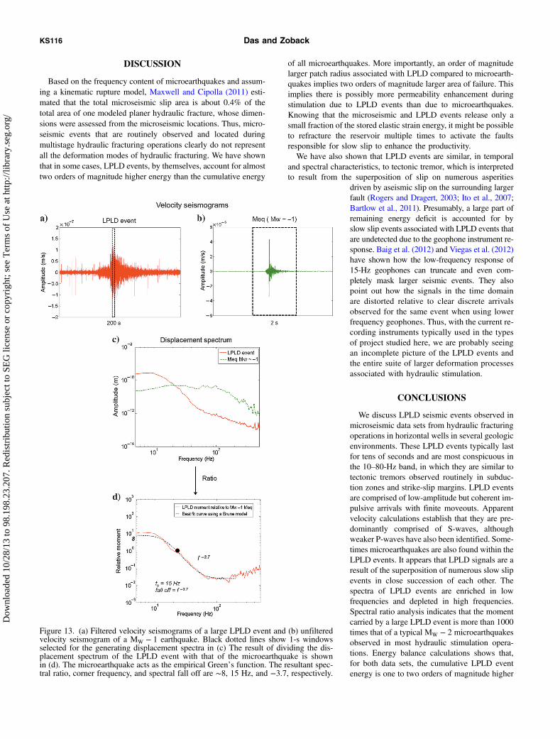
method (Frankel and Kanamori, 1983; Mori and Frankel, 1990;Venkataraman et al., 2002). In this method, a small earthquake lo-cated close to a larger earthquake is used as an EGF. The EGF isdeconvolved from the larger earthquake to remove the path and siteeffects and generate a clear source spectrum for the large earth-quake. In the frequency domain, this is just a simple division ofthe two amplitude spectra, and hence we call it the spectral ratio.The deconvolution assumes that the larger earthquake and smallerearthquake (LPLD event and microearthquake, in our case) arelocated close to each other such that the path effects are almostthe same for both events, which is a reasonable assumption for thisdata set.Figure 13a shows a filtered velocity seismogram for a relatively

large LPLD event (duration 50 s) from Barnett Data 2. Figure 13bshows the unfiltered velocity seismogram for a microearthquake(MW ∼ −1) from the same data set. Figure 13c shows the displace-ment spectra of the microearthquake and the LPLD event, calcu-lated by taking a 1-s time window as shown by dotted blacklines in Figure 13a and 13b. From the low-frequency amplitudelevel, it is clear that the microearthquake is significantly smaller

Figure 9. Top panels show the filtered seismograms of an LPLD event with progressively increasing time scales. Arrows delineate the low-amplitude precursor and the high-amplitude main event within a single LPLD event. Bottom panel shows the corresponding spectrograms withlow-amplitude, low-frequency, precursor followed by the high-amplitude, relatively high-frequency main event.

LPLD events: Waveform characteristics KS113

Dow

nloa

ded

10/2

8/13

to 9

8.19

8.23

.207

. Red

istr

ibut

ion

subj

ect t

o SE

G li

cens

e or

cop

yrig

ht; s

ee T

erm

s of

Use

at h

ttp://

libra

ry.s

eg.o

rg/

than the LPLD event; hence, it is an ideal candidate for the EGF. Inaddition, as explained in Das and Zoback (2013), this microearth-quake is in the general area in the reservoir where the LPLD event islocated, again satisfying the criteria of an EGF.In Figure 13d, we divided the low-frequency displacement am-

plitude spectrum of the LPLD event with that of displacement spec-trum of the microearthquake shown in Figure 13c to obtain themoment of the LPLD event relative to the moment of the micro-earthquake, which is known.Zhang et al. (2011) demonstrated that the displacement spectra of

the Cascadia tremors have corner frequencies around 3–8 Hz andfall off at f−2–f−3 at higher frequencies essentially agreeing withthe observations of regular earthquakes. Therefore, they suggestthat tremors could be analyzed using standard spectral models.Although we cannot be sure at this point whether tectonic tremorsand LPLD events are generated by similar mechanisms, due to theapparent similarity in waveforms (Figure 6) and in spectra(Figure 11), we consider it reasonable to use the standard modelsin our calculations, too. Therefore, we fit the resultant spectrumafter spectral division with a Brune (1970) source model to deter-mine the exact value of the relative moment and also the cornerfrequency. For this particular 1-s time window shown in Figure 13aand 13b, we estimate a spectral ratio of ∼8 which corresponds to amoment release rate of 2.5 × 108 N •m∕s for the LPLD event(Figure 13d). To get the cumulative moment of the entire LPLDevent, either we can take the summation of the spectral ratios fromeach 1-s windows for the entire duration of the LPLD event or wecan take the area under the displacement seismogram filtered from10-100 Hz (98% of the LPLD event energy). Both methods givevery similar results. From either method, we get a cumulative mo-ment of about 3 × 109 N •m. Using Hanks and Kanamori (1979),

MW ¼ 2

3× ðlog10MO − 9.1Þ; (3)

we calculate that this moment is equivalent to aMW ∼þ0.3 earthquake. It implies that a largeLPLD event has more than 1000 times the energyof a typical MW ∼ −2 microearthquake.As mentioned earlier, approximately 4500 mi-

croearthquakes were reported in Barnett Data 1ranging fromMW ∼ −1 to −4. In Barnett Data 2,there are about 7000 microearthquakes in themagnitude range from ∼ − 0.5 to −3. This indi-cates that just a few large LPLD events in eachdata set have more energy than all microearth-quakes recorded during the entire stimulation.Knowing the moments (approximately) of LPLDevents and microearthquakes, we can do a quan-titative analysis of the energy budget during hy-draulic stimulation.Maxwell et al. (2008), Maxwell (2010), Ci-

polla et al. (2011), and Warpinski et al. (2012)have already pointed out that the cumulative en-ergy of microearthquakes is a small fraction ofthe total injection energy and that slow, tensileopening and expansion of the hydraulic fractureaccounts for roughly 15%–20% of the injectionenergy.

Figure 10. (a) LPLD event observed during stage 7 of the simul-frac in Barnett Data 1. (b) A 0.3-s window of the filtered LPLDwaveform in (a) shown on an expanded time scale. Clear coherentlow-frequency impulsive arrival can be seen moving across the arrayshown by red dotted line. (c) Same timewindow as in (b), but withoutany filter applied. A microearthquake with clear P and S phases, dis-tinctly different from the low-frequency arrivals in Figure 9b, but withsimilar moveout, is found to occur within the LPLD event.

Figure 11. (a) Velocity spectrum of a large LPLD event of duration 50 s from BarnettData 2 (red solid line) compared with the spectrum of a MW − 0.5 microearthquake(blue dotted line) and a MW − 1.0 microearthquake (green dotted line), both∼450 m away from the recording geophones used for the calculation. The brown dottedline shows the background noise level. A multitaper spectral method was used to cal-culate the spectrum and a 1-s window was used in all cases. The instrument response ofthe 15-Hz recording geophones is shown by the black dotted line on top. (b) Velocityspectrum of tectonic tremor (black solid line), LFEs (gray solid line) and neighboringregular earthquakes greater thanMW > 2.5 (black dotted line) orMW < 2.5 (gray dottedline), all from western Shikoku in Japan (Shelly et al., 2007a). The thin gray dottedline shows the noise spectrum. Here, 2.5-s windows were used for all the spectrumcalculations.

KS114 Das and Zoback

Dow

nloa

ded

10/2

8/13

to 9

8.19

8.23

.207

. Red

istr

ibut

ion

subj

ect t

o SE

G li

cens

e or

cop

yrig

ht; s

ee T

erm

s of

Use

at h

ttp://

libra

ry.s

eg.o

rg/

It is also important to consider the microseismic and LPLDevents in terms of the relative amounts of elastic energy storedin the rock that they release. The amount of elastic strain energyin a volume of rock affected by stimulation that is available for shearslip on faults can be estimated from the deviatoric stresses in therock from the following equation (eq.–5.151 in Jaeger et al., 1969):

Ed ¼1

4G½ðs21 þ s22 þ s23Þ�; (4)

where Ed is the deviatoric strain energy density, G is the shear wavemodulus of the rock, and s1; s2, and s3 are the deviatoric stresses.Note that we have used the effective stresses to calculate the devia-toric stresses. For Barnett Data 1, we estimate the deviatoric strainenergy density to be 4.65 × 103 J∕m3 based on stress magnitudesand a value of 30 GPa for G based on observations of Sone (2012).From Figure 1, a conservative estimate of the volume of therock affected by stimulation for Barnett Data 1 is 1000 m ×700 m × 100 m. This gives us a total deviatoric stored energy of335 GJ. This amount of energy could potentially be released inthe form of shear slip events during stimulation.Summing up the moments of all the reported microearthquakes

yields 3.5 × 109 N · m. Using equation 2 (Kanamori and Anderson,1975), we estimate the elastic strain energy released by all micro-earthquakes together to be in the range of 3.5 × 106 J. Microearth-quakes that were not reported due to poor signal-to-noise ratio arenot expected to contribute significantly to the total moment becauseof their small size, as discussed previously. The sum of all LPLDmoments is about 150 × 109 N · m, which corresponds to energy inthe range of 150 × 106 J. This is a conservative estimate because welikely weren’t able to detect all the LPLD events because of theinstrument response of the 15-Hz sensors and overall low signal-to-noise ratio of the events. In addition, we only estimated the mo-ment from the portion of LPLD events that had distinct body wavephases. Nonetheless, the calculations tell us that for the entireBarnett Data 1, LPLD events released about 40 times as much en-ergy as the microearthquakes. Yet the LPLD events released onlyabout 0.05% of the total deviatoric strain energy stored in the res-ervoir prior to stimulation, compared with 0.001% released by themicroearthquakes.In Barnett Data 2, the total deviatoric strain energy in the volume

of the reservoir affected by the stimulation is esti-mated to be 285 × 109 J using the same calcula-tions as above. Nearly 50 LPLD events wereidentified in the entire operation, which is fewerthan the LPLD events identified in the BarnettData 1. Reported microearthquakes, on the otherhand, were almost double the number (and largerin size) than in Barnett Data 1. From the momentcalculations for this data set, it was found that themicroearthquakes released about 0.006% of thetotal deviatoric strain energy whereas LPLDevents released about 0.03%.Figure 13d also shows that the estimated cor-

ner frequency of the LPLD event is 15 Hz. Therange of corner frequency for all LPLD eventsobserved in the two data sets is from 10 to 20 Hz.Using Madariaga (1976),

r ¼ 0.21β

fc; (5)

where β is the shear-wave velocity and fc is the corner frequency,we get the radius of the fault patch to be in the range of 25–50 m fora corner-frequency range of 20–10 Hz. Using the Brune (1970)model would give us 1.76 times higher patch radius. However,the calculation is based on the assumption that rupture velocityis 0.9, which is most likely not true for LPLD events. Hence, thisestimated patch size should be treated as the upper limit. The micro-earthquakes with the range of magnitudes observed in the two datasets (−0.5 to −4) will rarely have corner frequencies below 100 Hzeven with stress drop as low as 0.1 MPa (Allman and Shearer,2009). Using the same equation 5, we get an upper limit of the patchsize radius of 4 m with the majority having radii less than a meter.Thus, compared to microearthquakes, LPLD events are associatedwith fault patches that are an order of magnitude larger.The estimates of corner frequencies of LPLD events (10–20 Hz)

are much lower than would be seen for regular earthquakes of com-parable seismic moment (Allman and Shearer, 2009). This obser-vation is consistent with those of Zhang et al. (2011), whofound that tremors and LFEs also have much lower corner frequen-cies for comparable moment. Two factors that might contribute tosuch low corner frequencies are very low stress drops and very lowrupture velocities. Using the stress-drop relation for a circular crackaccording to Eshelby (1957),

Δσ ¼ 7

16×M0 ×

�2 × π × fc2.34 × β

�3

; (6)

where Δσ is the stress drop, we get values ranging from 0.2 to 5 kPafor the LPLD events, much smaller than the 0.1–10 MPa of conven-tional earthquakes (Abercrombie and Leary, 1993; Allman andShearer, 2009). Low stress drop is most likely indicative of low ef-fective stress during rupture (Shelly et al., 2006; Audet et al., 2009),which is consistent with the fact that LPLD events occur in regionsof high fluid pressure during pumping, another topic addressed inDas and Zoback (2013).

Figure 12. Simplistic models of energy partitioning during earthquakes; ER is seismicradiation energy, EG is rupture energy, and EF is interface frictional energy. (a) Constantfriction model, in which fault stress drops to final value instantly and all the availableenergy is radiated as seismic energy. (b) Slip weakening model in which a portion of theavailable energy is used for rupture propagation, the rest is radiated as seismic energy.(c) Quasistatic model in which rupture is so slow that there is no radiated seismic energy.

LPLD events: Waveform characteristics KS115

Dow

nloa

ded

10/2

8/13

to 9

8.19

8.23

.207

. Red

istr

ibut

ion

subj

ect t

o SE

G li

cens

e or

cop

yrig

ht; s

ee T

erm

s of

Use

at h

ttp://

libra

ry.s

eg.o

rg/

DISCUSSION

Based on the frequency content of microearthquakes and assum-ing a kinematic rupture model, Maxwell and Cipolla (2011) esti-mated that the total microseismic slip area is about 0.4% of thetotal area of one modeled planer hydraulic fracture, whose dimen-sions were assessed from the microseismic locations. Thus, micro-seismic events that are routinely observed and located duringmultistage hydraulic fracturing operations clearly do not representall the deformation modes of hydraulic fracturing. We have shownthat in some cases, LPLD events, by themselves, account for almosttwo orders of magnitude higher energy than the cumulative energy

of all microearthquakes. More importantly, an order of magnitudelarger patch radius associated with LPLD compared to microearth-quakes implies two orders of magnitude larger area of failure. Thisimplies there is possibly more permeability enhancement duringstimulation due to LPLD events than due to microearthquakes.Knowing that the microseismic and LPLD events release only asmall fraction of the stored elastic strain energy, it might be possibleto refracture the reservoir multiple times to activate the faultsresponsible for slow slip to enhance the productivity.We have also shown that LPLD events are similar, in temporal

and spectral characteristics, to tectonic tremor, which is interpretedto result from the superposition of slip on numerous asperities

driven by aseismic slip on the surrounding largerfault (Rogers and Dragert, 2003; Ito et al., 2007;Bartlow et al., 2011). Presumably, a large part ofremaining energy deficit is accounted for byslow slip events associated with LPLD events thatare undetected due to the geophone instrument re-sponse. Baig et al. (2012) and Viegas et al. (2012)have shown how the low-frequency response of15-Hz geophones can truncate and even com-pletely mask larger seismic events. They alsopoint out how the signals in the time domainare distorted relative to clear discrete arrivalsobserved for the same event when using lowerfrequency geophones. Thus, with the current re-cording instruments typically used in the typesof project studied here, we are probably seeingan incomplete picture of the LPLD events andthe entire suite of larger deformation processesassociated with hydraulic stimulation.

CONCLUSIONS

We discuss LPLD seismic events observed inmicroseismic data sets from hydraulic fracturingoperations in horizontal wells in several geologicenvironments. These LPLD events typically lastfor tens of seconds and are most conspicuous inthe 10–80-Hz band, in which they are similar totectonic tremors observed routinely in subduc-tion zones and strike-slip margins. LPLD eventsare comprised of low-amplitude but coherent im-pulsive arrivals with finite moveouts. Apparentvelocity calculations establish that they are pre-dominantly comprised of S-waves, althoughweaker P-waves have also been identified. Some-times microearthquakes are also found within theLPLD events. It appears that LPLD signals are aresult of the superposition of numerous slow slipevents in close succession of each other. Thespectra of LPLD events are enriched in lowfrequencies and depleted in high frequencies.Spectral ratio analysis indicates that the momentcarried by a large LPLD event is more than 1000times that of a typical MW − 2 microearthquakesobserved in most hydraulic stimulation opera-tions. Energy balance calculations shows that,for both data sets, the cumulative LPLD eventenergy is one to two orders of magnitude higher

Figure 13. (a) Filtered velocity seismograms of a large LPLD event and (b) unfilteredvelocity seismogram of a MW − 1 earthquake. Black dotted lines show 1-s windowsselected for the generating displacement spectra in (c) The result of dividing the dis-placement spectrum of the LPLD event with that of the microearthquake is shownin (d). The microearthquake acts as the empirical Green’s function. The resultant spec-tral ratio, corner frequency, and spectral fall off are ∼8, 15 Hz, and −3.7, respectively.

KS116 Das and Zoback

Dow

nloa

ded

10/2

8/13

to 9

8.19

8.23

.207

. Red

istr

ibut

ion

subj

ect t

o SE

G li

cens

e or

cop

yrig

ht; s

ee T

erm

s of

Use

at h

ttp://

libra

ry.s

eg.o

rg/

than the cumulative energy of microearthquakes. Further, slow slipon large-scale faults, which is inferred to accompany LPLD events,appears to be a significant process during hydraulic stimulation.

ACKNOWLEDGMENTS

We are grateful to ConocoPhillips Company, BP, Apache, andEncana for providing the data used in this research. We also wishto thank Pinnacle — a Halliburton service — for technical support.ConocoPhillips, Chevron, the Stanford Rock and Borehole Geo-physics industrial affiliates program, and an SEG Foundation Schol-arship provided funding for this research.

REFERENCES

Abercrombie, R., and P. Leary, 1993, Source parameters of small earth-quakes recorded at 2.5 km depth, Cajon Pass, Southern California:Implications for earthquake scaling: Geophysical Research Letters, 20,1511–1514, doi: 10.1029/93GL00367.

Aki, K., 1967, Scaling law of seismic spectrum: Journal of Geophysical Re-search, 72, 1217–1231, doi: 10.1029/JZ072i004p01217.

Allman, B. P., and P. M. Shearer, 2009, Global variations of stress drop formoderate to large earthquakes: Journal of Geophysical Research, 114,B01310, doi: 10.1029/2008JB005821.

Audet, P., M. G. Bostock, N. I. Christensen, and S. M. Peacock, 2009, Seis-mic evidence for overpressured subducted oceanic crust and megathrustfault sealing: Nature, 457, 76–78, doi: 10.1038/nature07650.

Baig, A. M., T. Urbancic, and G. Viegas, 2012, Do hydraulic fractures in-duce events large enough to be felt on the surface?: CSEG Recorder, 10,40–46.

Bartlow, N. M., S. Miyazaki, A. M. Bradley, and P. Segall, 2011, Space-timecorrelation of slip and tremor during the 2009 Cascadia slow slip event:Geophysical Research Letters, 38, L18309, doi: 10.1029/2011GL048714.

Brown, J. R., G. C. Beroza, S. Ide, K. Ohta, D. R. Shelly, S. Y. Schwartz, W.Rabbel, M. Thorwart, and H. Kao, 2009, Deep low-frequencyearthquakes in tremor localize to the plate interface in multiple subductionzones: Geophysical Research Letters, 36, L19306, doi: 10.1029/2009GL040027.

Brune, J., 1970, Tectonic stress and the spectra of seismic shear waves fromearthquakes: Journal of Geophysical Research, 75, 4997–5009, doi: 10.1029/JB075i026p04997.

Cipolla, C. L., S. Maxwell, M. Mack, and R. Downie, 2011, A practicalguide to interpreting microseismic measurements: Proceedings: Societyof Petroleum Engineers North American Unconventional Gas Conferenceand Exhibition, Paper 144067.

Das, I., and M. D. Zoback, 2011, Long period long duration seismic eventsduring hydraulic fracture stimulation of a shale gas reservoir: The LeadingEdge, 30, 778–786, doi: 10.1190/1.3609093.

Das, I., and M. D. Zoback, 2013, Long-period long-duration seismic eventsduring hydraulic stimulation of shale and tight gas reservoirs — Part 2:Location and mechanisms: Geophysics, 78, this issue, doi: 10.1190/GEO2013-0165.1.

Eaton, D., M. Van der Baan, J. B. Tary, B. Birkelo, N. Spriggs, S. Cutten, andK. Pike, 2013, Broadband microseismic observations from a Montneyhydraulic fracture treatment, northeastern British Columbia: CSEGRecorder, 38, 45–53.

Eshelby, J. D., 1957, The determination of the elastic field of an ellipsoidalinclusion, and related problems: Proceedings of the Royal Society of Lon-don, Series A: Mathematical, Physical and Engineering Sciences, 241,376–396, doi: 10.1098/rspa.1957.0133.

Frankel, A., and H. Kanamori, 1983, Determination of rupture duration andstress drop for earthquakes in southern California: Bulletin of theSeismological Society of America, 73, 1527–1551.

Geiser, P., A. Lacazette, and J. Vermilye, 2012, Beyond ‘dots in a box’: Anempirical view of reservoir permeability with tomographic fracture imag-ing: First Break, 30, 63–69.

Hanks, T., and H. Kanamori, 1979, A moment magnitude scale: Journal ofGeophysical Research, 84, 2348–2350, doi: 10.1029/JB084iB05p02348.

Hirose, H., and K. Obara, 2010, Recurrence behavior of short-term slow slipand correlated nonvolcanic tremor episodes in western Shikoku, south-west Japan: Journal of Geophysical Research, 115, B00A21, doi: 10.1029/2008JB006050.

Hirose, T., Y. Hiramatsu, and K. Obara, 2010, Characteristics of short-termslow slip events estimated from deep low-frequency tremors in Shikoku,Japan: Journal of Geophysical Research, 115, B10304, doi: 10.1029/2010JB007608.

Hurd, O., and M. D. Zoback, 2012, Stimulated shale volume characteriza-tion: Multiwell case study from the Horn River Shale: Part 1: Geome-chanics and microseismicity: Annual Technical Conference, SPE,Paper 159536.

Ide, S., G. C. Beroza, D. R. Shelly, and T. Uchide, 2007, A scaling law forslow earthquakes: Nature, 447, 76–79, doi: 10.1038/nature05780.

Ito, Y., K. Obara, K. Shiomi, S. Sekine, and H. Hirose, 2007, Slow earth-quakes coincident with episodic tremors and slow slip events: Science,315, 503–506, doi: 10.1126/science.1134454.

Jaeger, J. C., N. G. W. Cook, and R. W. Zimmerman, 1969, Fundamentals ofrock mechanics.

Julian, B., 1994, Volcanic tremor: Nonlinear excitation by fluid flow: Journalof Geophysical Research, 99, 11859–11877, doi: 10.1029/93JB03129.

Kanamori, H., and D. L. Anderson, 1975, Theoretical basis of some empiri-cal relations in seismology: Bulletin of the Seismological Society ofAmerica, 65, 1073–1095.

Kanamori, H., and L. Rivera, 2006, Energy partitioning during an earth-quake: AGU Chapman Volume, Geophysical Monograph Series 170,“Earthquakes: Radiated Energy and the Physics of Faulting”.

Kim, M. J., S. Y. Schwartz, and S. Bannister, 2011, Non-volcanic tremorassociated with the March 2010 Gisborne slow slip event at the Hikurangisubduction margin, New Zealand: Geophysical Research Letters, 38,L14301.

Konstantinou, K. I., and V. Schlindwein, 2003, Nature, wavefield propertiesand source mechanism of volcanic tremor: A review: Journal of Volcan-ology and Geothermal Research, 119, 161–187, doi: 10.1016/S0377-0273(02)00311-6.

La Rocca, M., K. C. Creager, D. Galluzzo, S. Malone, J. E. Vidale, J. R.Sweet, and A. G. Wech, 2009, Cascadia tremor located near plate inter-face constrained by S minus P-wave times: Science, 323, 620–623, doi:10.1126/science.1167112.

Madariaga, R., 1976, Dynamics of an expanding circular fault: Bulletin ofthe Seismological Society of America, 66, 639–666.

Maxwell, S. C., 2010, Microseismic growth born from success: The LeadingEdge, 29, 338–343, doi: 10.1190/1.3353732.

Maxwell, S. C., and C. Cipolla, 2011, What does microseismicity tell usabout hydraulic fracturing?: Annual Technical Conference, SPE, Paper146932.

Maxwell, S. C., J. Shemeta, E. Campbell, and D. Quirk, 2008, Microseismicdeformation rate monitoring: Annual Technical Conference, SPE, Paper116596.

Moos, D., G. Vassilellis, R. Cade, J. Franquet, A. Lacazette, E. Bourtem-bourg, and R. Cade, 2011, Predicting shale reservoir response to stimu-lation in the upper Devonian of West Virginia: Annual TechnicalConference, SPE, Paper 145849.

Mori, J., and A. Frankel, 1990, Source parameters for small events associ-ated with the 1986 North Palm Springs, California, earthquake determinedusing empirical Green functions: Bulletin of the Seismological Society ofAmerica, 80, 278–295.

Nadeau, R. M., and A. Guilhem, 2009, Nonvolcanic tremor evolution andthe San Simeon and Parkfield, California, Earthquakes: Science, 325,191–193, doi: 10.1126/science.1174155.

Obara, K., 2002, Nonvolcanic deep tremor associated with subduction inSouthwest Japan: Science, 296, 1679–1681, doi: 10.1126/science.1070378.

Obara, K., H. Hirose, F. Yamamizu, and K. Kasahara, 2004, Episodic slowslip events accompanied by non-volcanic tremors in southwest Japan sub-duction zone: Geophysical Research Letters, 31, L23602, doi: 10.1029/2004GL020848.

Riuscetti, M., R. Schick, and D. Seidl, 1977, Spectral parameters of volcanictremors at Etna: Journal of Volcanology and Geothermal Research, 2,289–298, doi: 10.1016/0377-0273(77)90004-X.

Rogers, G., and H. Dragert, 2003, Episodic tremor and slip on the Cascadiasubduction zone: The chatter of silent slip: Science, 300, 1942–1943, doi:10.1126/science.1084783.

Rutledge, J. T., and W. S. Phillips, 2003, Hydraulic stimulation of naturalfractures as revealed by induced microearthquakes, Carthage CottonValley gas field, East Texas: Geophysics, 68, 441–452, doi: 10.1190/1.1567214.

Shelly, D. R., 2010, Migrating tremors illuminate complex deformation be-neath the seismogenic San Andreas fault: Nature, 463, 648–652, doi: 10.1038/nature08755.

Shelly, D. R., and G. C. Beroza, 2007b, Complex evolution of transientslip derived from precise tremor locations in western Shikoku, Japan:Geochemistry, Geophysics, Geosystems, 8, Q10014, doi: 10.1029/2007GC001640.

Shelly, D. R., G. C. Beroza, and S. Ide, 2007a, Non-volcanic tremor and low-frequency earthquake swarms: Nature, 446, 305–307, doi: 10.1038/nature05666.

Shelly, D. R., G. C. Beroza, S. Ide, and S. Nakamuta, 2006, Low-frequencyearthquakes in Shikoku, Japan, and their relationship to episodic tremorand slip: Nature, 442, 188–191, doi: 10.1038/nature04931.

LPLD events: Waveform characteristics KS117

Dow

nloa

ded

10/2

8/13

to 9

8.19

8.23

.207

. Red

istr

ibut

ion

subj

ect t

o SE

G li

cens

e or

cop

yrig

ht; s

ee T

erm

s of

Use

at h

ttp://

libra

ry.s

eg.o

rg/

Shelly, D. R., and J. L. Hardebeck, 2010, Precise tremor source locationsand amplitude variations along the lower-crustal central San AndreasFault: Geophysical Research Letters, 37, L14301, doi: 10.1029/2010GL043672.

Sicking, C., J. Vermiliye, P. Geiser, A. Lacazette, and L. Thompson, 2013,Permeability field imaging from microseismic: Geophysical Society ofHouston Journal, 3, 11–14.

Sone, H., 2012, Mechanical properties of shale gas reservoir rocks and itsrelation to the in-situ stress variation observed in shale gas reservoirs:Ph.D. thesis, Stanford.

Venkataraman, A., L. Rivera, and H. Kanamori, 2002, Radiated energy fromthe 16 October 1999 Hector Mine Earthquake: Regional and teleseismicestimates: Bulletin of the Seismological Society of America, 92, 1256–1265, doi: 10.1785/0120000929.

Vermylen, J. P., andM. D. Zoback, 2011, Hydraulic fracturing, microseismicmagnitudes, and stress evolution in the Barnett Shale, Texas, USA: An-nual Technical Conference, SPE, Paper 140507.

Viegas, G., A. Baig, W. Coulter, and T. Urbancic, 2012, Effective monitoringof reservoir-induced seismicity utilizing integrated surface and downholeseismic networks: First Break, 30, 77–81.

Warpinski, N. R., J. Du, and U. Zimmer, 2012, Measurements of hydraulic-fracture-induced seismicity in gas shales: Hydraulic Fracturing Technol-ogy Conference, SPE, Paper 151597.

Warpinski, N. R., S. L. Wolhart, and C. A. Wright, 2004, Analysis and pre-diction of microseismicity induced by hydraulic fracturing: Society ofPetroleum Engineers Journal, 9, 24–33.

Zhang, J., P. Gerstoft, P. M. Shearer, H. Yao, J. E. Vidale, H. Houston, and A.Ghosh, 2011, Cascadia tremor spectra: Low corner frequencies and earth-quake-like high-frequency falloff: Geochemistry, Geophysics, Geosys-tems, 12, Q10007.

Zoback, M. D., A. Kohli, I. Das, and M. McClure, 2012, The importance ofslow slip on faults during hydraulic fracturing stimulation of shale gasreservoirs: Americas Unconventional Resources Conference, SPE, Paper155476.

KS118 Das and Zoback

Dow

nloa

ded

10/2

8/13

to 9

8.19

8.23

.207

. Red

istr

ibut

ion

subj

ect t

o SE

G li

cens

e or

cop

yrig

ht; s

ee T

erm

s of

Use

at h

ttp://

libra

ry.s

eg.o

rg/