Lone Wolves in Competitive Equilibria

Ravi Jagadeesan Scott Duke Kominers Ross Rheingans-Yoo

Working Paper 18-055

Working Paper 18-055

Copyright © 2017 by Ravi Jagadeesan, Scott Duke Kominers, and Ross Rheingans-Yoo

Working papers are in draft form. This working paper is distributed for purposes of comment and discussion only. It may not be reproduced without permission of the copyright holder. Copies of working papers are available from the author.

Lone Wolves in Competitive Equilibria Ravi Jagadeesan Harvard University

Scott Duke Kominers Harvard Business School

Ross Rheingans-Yoo Harvard University

Lone Wolves in Competitive Equilibria∗

Ravi JagadeesanDepartment of Mathematics

Harvard UniversityScott Duke Kominers

Harvard Business School and Department of EconomicsHarvard UniversityRoss Rheingans-Yoo

Center of Mathematical Sciences and ApplicationsHarvard University

December 23, 2017

Abstract

This paper develops a class of equilibrium-independent predictions of competitiveequilibrium with indivisibilities. Specifically, we prove an analogue of the “Lone WolfTheorem” of classical matching theory, showing that when utility is perfectly transferable,any agent who does not participate in trade in one competitive equilibrium must receiveher autarky payoff in every competitive equilibrium. Our results extend to approximateequilibria and to settings in which utility is only approximately transferable.

JEL Classification: C78, D47, D51

Keywords: Indivisibilities; Matching; Lone Wolf Theorem

∗This paper was previously circulated under the more amusing title, “If You’re Happy and You Know ItThen You’re Matched.” This research was conducted while Jagadeesan and Rheingans-Yoo were EconomicDesign Fellows at the Harvard Center of Mathematical Sciences and Applications (CMSA). The authors thankMohammad Akbarpour, John William Hatfield, Shengwu Li, Paul Milgrom, Robbie Minton, Casey Mulligan,Alvin E. Roth, and Alexander Teytelboym for helpful comments. Jagadeesan gratefully acknowledges travelsupport from the Harvard Business School and the Harvard Mathematics Department. Kominers gratefullyacknowledges the support of National Science Foundation grant SES-1459912 and the Ng Fund of the CMSA.

1

1 Introduction

In models of exchange and production, results on the uniqueness of equilibria typically require

continuity and convexity conditions on agents’ preferences, in addition to further conditions

on aggregate demand (see, for example, Section 17.F of Mas-Colell et al. (1995)). However,

continuity and convexity conditions fail in the presence of indivisibilities, leading to the

existence of multiple equilibria. In turn, the presence of multiple equilibria weakens the

predictive power of economic models.

To avoid the problems of multiplicity, we often consider predictions that do not depend on

which equilibrium is realized.1 In this paper, we develop a class of equilibrium-independent

predictions of competitive equilibrium in exchange economies with indivisibilities.2 Specifically,

we show that when utility is perfectly transferable, any agent who does not participate in

trade in one competitive equilibrium must receive her autarky payoff in every competitive

equilibrium. Hence, observing that an agent does not participate in trade indicates that there

is no competitive equilibrium in which that agent improves on her autarky payoff.

Our result is analogous to the classical “Lone Wolf Theorem” in matching theory, which

asserts that in one-to-one matching without transfers, any agent who is unmatched in some

stable outcome is unmatched in every stable outcome (McVitie and Wilson (1970)). Informally,

the Lone Wolf Theorem shows the set of “lone wolves” (unmatched agents) is equilibrium-

independent. Since our setting involves continuous transfers, and hence indifferences, we

cannot obtain sharp predictions regarding the set of agents that participate in trade in

equilibrium. Instead, we show that any agent who does not participate in trade in one

equilibrium cannot benefit from trade in any equilibrium.1In structural estimation, for example, it is possible to avoid the problem of multiplicity of equilibria by

performing inference based on equilibrium-independent predictions of the model (see, for example, Bresnahanand Reiss (1991)). A realted alternative approach, which is valid even when there are few equilibrium-independent predictions, is to obtain set-identification of the parameters of interest by assuming that theobservation is one of many possible equilibria (see, for example, Tamer (2003); Ciliberto and Tamer (2009);Pakes (2010); Galichon and Henry (2011); Pakes et al. (2015); Bontemps and Magnac (2017)).

2We use the Baldwin and Klemperer (2015) model, which the nests the models of Gul and Stacchetti(1999) and Sun and Yang (2006), as well as the Hatfield et al. (2013) model of matching in trading networkswith transferable utility.

2

When utility is perfectly transferable, there is generically a unique efficient allocation of

goods among agents, although there may be multiple possible equilibrium price vectors. Hence,

the set of agents that participate in trade is generically equilibrium-independent. However,

our lone wolf result applies even when there are multiple efficient allocations. Moreover, we

show that versions of our Lone Wolf Theorem hold in settings in which multiple allocations

can be robustly sustained in equilibrium. Specifically, we consider an approximate equilibrium

concept—which may be a reasonable solution when the economy suffers from small frictions—

and derive an approximate Lone Wolf Theorem. We also prove an approximate Lone Wolf

Theorem for equilibria in economies in which utility is only approximately transferable among

agents.

Quasi-conversely, we show that some assumption on the transferability of utility is

essential to our lone wolf results. Specifically, we show by example that lone wolf results

do not hold in settings with strong income effects. Hence, while our lone wolf results show

that competitive equilibrium has some (approximately) robust predictions when utility is

(approximately) transferable, it remains an open question whether we can derive specific

classes of equilibrium-independent predictions more generally.3

In a companion paper (Jagadeesan et al. (2017)), we use our Lone Wolf Theorem to

show that descending salary-adjustment processes are strategy-proof in quasilinear Kelso and

Crawford (1982) economies. Our argument for strategy-proofness rests crucially on applying

our Lone Wolf Theorem to (non-generic) economies with multiple efficient matchings.

The remainder of this paper is organized as follows. Section 2 presents the model. Section 3

presents our lone wolf results. Section 4 discusses the role of the hypothesis that utility

is (approximately) transferable. Section 5 connects our results to the matching literature.

Proofs omitted from the main text are presented in Appendix A.3In this context, an agent that does not participate in trade may seek to change the equilibrium selection

in order to improve her payoff, which may be possible in the presence of income effects.

3

2 Model

We consider a general model of exchange economies with indivisible goods and transferable

utility, following Baldwin and Klemperer (2015); this framework embeds the trading network

model of Hatfield et al. (2013), which in turn generalizes the settings of Gul and Stacchetti

(1999, 2000) and Sun and Yang (2006, 2009). There is a set Γ of goods and a finite set I of

agents.

Each agent has an endowment ei ∈ ZΓ and a valuation

vi : ZΓ → R ∪ {−∞}.

We assume that valuations are bounded above; however, we do not impose any further

conditions on them. The valuation vi induces a quasilinear utility function ui by

ui(qi; ti) = vi(qi) + ti.

A competitive equilibrium is comprised of (1) an allocation of goods to agents and (2)

prices for each good such that the allocation maximizes each agent’s utility given prices.

Definition 1. A competitive equilibrium is a pair [q; p] at which

• each agent i demands her allocation qi at prevailing prices p, i.e.,

qi ∈ arg maxqi∈ZΓ

{ui(q i; (ei − q i) · p)

}(1)

for all i ∈ I, and

• the market clears, i.e., ∑i∈I

qi =∑i∈I

ei. (2)

Remark. Although our model formally requires that goods be indivisible, our results apply in

4

settings with divisible goods as well.

3 Results

The classical Lone Wolf Theorem from the theory of two-sided matching without transfers

asserts that any agent who is matched in some equilibrium outcome is matched in every

equilibrium (McVitie and Wilson (1970); see also Roth (1984, 1986)). In this section, we

prove analogues of the Lone Wolf Theorem for exchange economies.

3.1 An Exact Lone Wolf Theorem

For a pair [q; p], we say that an agent i ∈ I does not participate in trade in [q; p] if qi = ei.

Such an agent is a “lone wolf” in [q; p] .

Our first result asserts that any agent who does not participate in trade in some competitive

equilibrium receives her autarky payoff in every competitive equilibrium. Thus, we show

that any agent who is a “lone wolf” in some equilibrium cannot benefit from trade in any

equilibrium.

Theorem 1. Let [q; p] and [q ; p] be competitive equilibria, and let j ∈ I be an agent. If

j does not participate in trade in [q ; p] (i.e., if qj = ej), then uj(qj; tj) = uj(ej; 0), where

tj = (ej − qj) · p.

The key to the proof of Theorem 1 is the following lemma, which allows us to produce a

new competitive equilibrium from any two competitive equilibria.

Lemma 1 (Shapley (1964); Hatfield et al. (2013)). If [q; p] and [q ; p] are competitive equilibria,

then [q ; p] is a competitive equilibrium.

To prove Theorem 1, we exploit the fact that [q ; p] is a competitive equilibrium (by

Lemma 1), so the allocation q must maximize j’s utility given the price vector p.

5

Proof of Theorem 1. By Lemma 1, [q ; p] is a competitive equilibrium. Since both [q; p] and

[q ; p] are competitive equilibria, every agent i must be indifferent between consumption

bundles qi and q i at price vector p. In particular, j must be indifferent between consumption

bundles qj and ej = qj at price vector p. Formally, we have that

uj(qj; tj) = uj(qj; (ej − qj) · p) = uj(ej; (ei − ej) · p) = uj(ej; 0),

as claimed.

3.2 An Approximate Lone Wolf Theorem

Note that Theorem 1 applies only in economies in which there are multiple efficient allocations.

As efficient allocations are generically unique in transferable utility economies, Theorem 1

has nontrivial consequences only for nongeneric economies.

However, as we show in this section, our lone wolf result holds more generally. In particular,

we prove a version of Theorem 1 for approximate equilibria; as approximate equilibria are

only approximately efficient, this result has nontrivial consequences in settings in which

equilibrium allocations are robustly non-unique.

We relax the notion of competitive equilibrium by allowing agents’ total maximization

error to be positive but bounded above by ε.

Definition 2. An ε-equilibrium consists of a pair [q; p] for which

∑i∈I

(maxqi∈ZΓ

ui(q i; (ei − q i) · p)− ui(qi; (ei − qi) · p)) ≤ ε

and (2) is satisfied (i.e., the market clears).

Our Approximate Lone Wolf Theorem asserts that if there exists an ε-equilibrium in

which no agents in J ⊆ I participate in trade, then the difference between the total utility of

agents in J and the total autarky payoff of agents in J is bounded above by (δ + ε) in every

6

δ-equilibrium.

Theorem 2. Let [q; p] be a δ-equilibrium, let [q ; p] be an ε-equilibrium, and let J ⊆ I be a

set of agents. If no agent in J participates in trade in [q ; p] (i.e., if qj = ej for all j ∈ J),

then ∑j∈J

uj(qj; tj)−∑j∈J

uj(ej; 0) ≤ δ + ε,

where tj = (ej − qj) · p.

The proof of Theorem 2 is similar to the proof of Theorem 1, but relies on an approximate

version of Lemma 1.

Taking J = {j} yields the following corollary, which corresponds more directly to

Theorem 1.

Corollary 1. Let [q; p] be a δ-equilibrium, let [q ; p] be an ε-equilibrium, and let j ∈ I be an

agent. If j does not participate in trade in [q ; p] (i.e., if qj = ej), then

uj(qj; tj)− uj(ej; 0) ≤ δ + ε,

where tj = (ej − qj) · p.

3.3 A Lone Wolf Theorem for Economies with Approximately

Transferable Utility

Theorem 2 also implies a Lone Wolf Theorem for economies in which utility is “close to

transferable” in a formal sense. Specifically, we consider economies in which agents’ utility

functions can be well-approximated by quasilinear utility functions.

Definition 3. A utility function ui is quasilinear within η if there exists a quasilinear utility

function ui for which

supqi,ti

{∣∣∣ui(qi; ti)− ui(qi; ti)∣∣∣} ≤ η.

7

When utility functions are approximately quasilinear, we obtain an approximate Lone

Wolf Theorem.

Theorem 3. Let [q; p] and [q ; p] be competitive equilibria, and let J ⊆ I be a set of agents. If

no agent in J participates in trade in [q ; p] (i.e., if qj = ej for all j ∈ J) and ui is quasilinear

within η for all i ∈ I, then

∑j∈J

uj(qj; tj)−∑j∈J

uj(ej; 0) ≤ 6η|I|,

where tj = (ej − qj) · p.

To prove Theorem 3, we construct an approximating economy in which utility functions

are quasilinear. Competitive equilibria in the original economy give rise to approximate

equilibria in the approximating economy; Theorem 3 then follows from Theorem 2.

Proof of Theorem 3. We define an auxiliary economy in which utility functions are given

by (ui)i∈I , with each ui quasilinear as in Definition 3. By construction, [q; p] and [q ; p] are

2η|I|-equilibria in the auxiliary economy. Theorem 2 then guarantees that

∑j∈J

uj(qj; tj)−∑j∈J

uj(ej; 0) ≤ 4η|I|. (3)

As ∑j∈J |uj(qj; tj)− uj(qj; tj)| ≤ η|I| and ∑j∈J |uj(ej; 0)− uj(ej; 0)| ≤ η|I| by our choice of

(ui)i∈I , we see from (3) that

∑j∈J

uj(qj; tj)−∑j∈J

uj(ej; 0) ≤ 6η|I|,

as desired.

8

4 The Role of Utility Transferability

The proofs of our Lone Wolf Theorems use the assumption that utility is (at least approxi-

mately) transferable. In fact, the Lone Wolf Theorem fails when utility is not transferable,

such as in the presence of income effects.

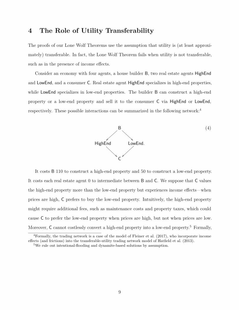
Consider an economy with four agents, a house builder B, two real estate agents HighEnd

and LowEnd, and a consumer C. Real estate agent HighEnd specializes in high-end properties,

while LowEnd specializes in low-end properties. The builder B can construct a high-end

property or a low-end property and sell it to the consumer C via HighEnd or LowEnd,

respectively. These possible interactions can be summarized in the following network:4

B

~~ HighEnd

LowEnd.

~~C

(4)

It costs B 110 to construct a high-end property and 50 to construct a low-end property.

It costs each real estate agent 0 to intermediate between B and C. We suppose that C values

the high-end property more than the low-end property but experiences income effects—when

prices are high, C prefers to buy the low-end property. Intuitively, the high-end property

might require additional fees, such as maintenance costs and property taxes, which could

cause C to prefer the low-end property when prices are high, but not when prices are low.

Moreover, C cannot costlessly convert a high-end property into a low-end property.5 Formally,4Formally, the trading network is a case of the model of Fleiner et al. (2017), who incorporate income

effects (and frictions) into the transferable-utility trading network model of Hatfield et al. (2013).5We rule out intentional-flooding and dynamite-based solutions by assumption.

9

C has utility function

uC(high-end property, t) = 2t+ 600

uC(low-end property, t) = t+ 400.

As there is only one real estate agent of each type (or, more generally, as we do not

assume that there is free entry in the markets for real estate agents), it may be possible for

the real estate agents to extract rents. Thus, a competitive equilibrium must specify prices

that the consumer faces for each type of property separately from the prices that real estate

agents face.

There are two possible equilibrium allocations: either B can construct a high-end property

and sell it to C via HighEnd, or B can construct a low-end property and sell it to C via

LowEnd. For example, two competitive equilibria are:

B115~~

50��

B152~~

95

HighEnd

120

LowEnd

50��

and HighEnd

152

LowEnd.

100~~C C

(A) (B)

(Here, we denote competitive equilibria by writing a price for each interaction in (4) and

boxing the prices of interactions that occur.) In Equilibrium (A), HighEnd extracts a rent of

5 from intermediating between B and C; in Equilibrium (B), LowEnd extracts a rent of 5 from

intermediating. However, HighEnd does not trade in Equilibrium (B), while LowEnd does not

trade in Equilibrium (A). Thus, there are agents who do not trade in one equilibrium but

receive utility strictly greater than their autarky payoffs in the other equilibrium—that is,

the lone wolf result fails.

10

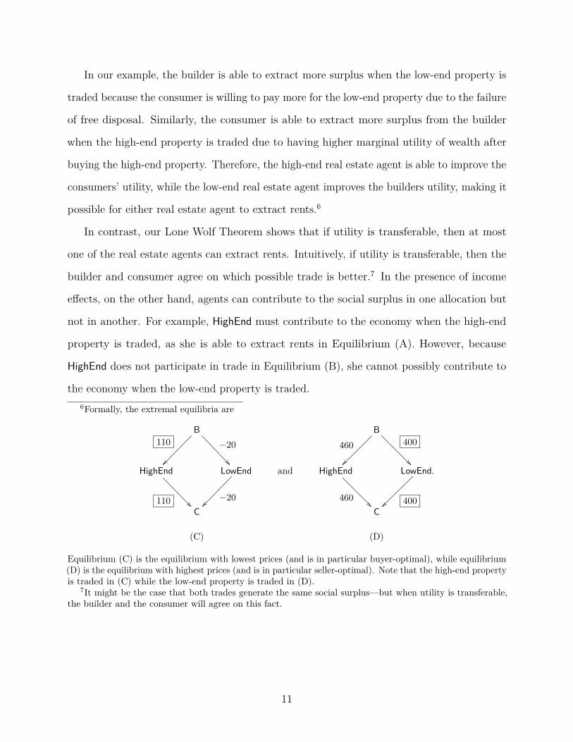
In our example, the builder is able to extract more surplus when the low-end property is

traded because the consumer is willing to pay more for the low-end property due to the failure

of free disposal. Similarly, the consumer is able to extract more surplus from the builder

when the high-end property is traded due to having higher marginal utility of wealth after

buying the high-end property. Therefore, the high-end real estate agent is able to improve the

consumers’ utility, while the low-end real estate agent improves the builders utility, making it

possible for either real estate agent to extract rents.6

In contrast, our Lone Wolf Theorem shows that if utility is transferable, then at most

one of the real estate agents can extract rents. Intuitively, if utility is transferable, then the

builder and consumer agree on which possible trade is better.7 In the presence of income

effects, on the other hand, agents can contribute to the social surplus in one allocation but

not in another. For example, HighEnd must contribute to the economy when the high-end

property is traded, as she is able to extract rents in Equilibrium (A). However, because

HighEnd does not participate in trade in Equilibrium (B), she cannot possibly contribute to

the economy when the low-end property is traded.6Formally, the extremal equilibria are

B110

��

−20

��

B460

��

400

��HighEnd

110 ��

LowEnd

−20��

and HighEnd

460��

LowEnd.

400��C C

(C) (D)

Equilibrium (C) is the equilibrium with lowest prices (and is in particular buyer-optimal), while equilibrium(D) is the equilibrium with highest prices (and is in particular seller-optimal). Note that the high-end propertyis traded in (C) while the low-end property is traded in (D).

7It might be the case that both trades generate the same social surplus—but when utility is transferable,the builder and the consumer will agree on this fact.

11

5 Discussion and Conclusion

We developed a class of Lone Wolf Theorems that provide equilibrium-independent predictions

of competitive equilibrium analysis in contexts with indivisibilities. Our results show that

when utility is perfectly transferable, any agent who does not participate in trade in one

competitive equilibrium must receive her autarky payoff in every competitive equilibrium;

moreover, this result holds approximately under approximate solution concepts and in settings

in which utility is only approximately transferable. Partial transferability of utility is essential

for our results—the lone wolf conclusion fails when utility is not transferable (e.g., in the

presence of income effects).

5.1 Relationship to the Lone Wolf Theorems and Rural Hospitals

Theorems of Matching Theory

Our lone wolf results extend a classical matching-theoretic insight of McVitie and Wilson

(1970) to exchange economies. Other analogues of the Lone Wolf Theorem have been

developed in matching, but those results have different hypotheses and conclusions from ours.

The most-general matching-theoretic generalizations—developed by Hatfield and Kominers

(2012) and Fleiner, Jankó, Tamura, and Teytelboym (2015)—state that for every agent in a

trading network (without transfers), the difference between the numbers of the goods bought

and sold is invariant across stable outcomes.8 Our results extend the Lone Wolf Theorem to

exchange economies (with transfers) by assessing when agents participate in (profitable) trade

instead of analyzing the amounts that agents trade. Furthermore, the matching-theoretic

results rely on two regularity conditions—some form of (gross) substitutability (Kelso and8These results are typically called Rural Hospitals Theorems because they imply that that clearinghouses

cannot improve the recruitment total of rural hospitals—which are often less attractive to doctors—byswitching to different (stable) market-clearing mechanisms. The first Rural Hospitals Theorems were provenby Roth (1984, 1986) for many-to-one matching with responsive preferences. Rural Hospitals Theorems werealso developed for many-to-many matching (Alkan (2002); Klijn and Yazıcı (2014)), many-to-one matchingwith contracts (Hatfield and Milgrom (2005); Hatfield and Kojima (2010)), and many-to-many matching withcontracts (Hatfield and Kominers (2017)).

12

Crawford, 1982), and a regularity condition called the “law of aggregate demand”9—which

we do not require. We instead require that utility is at least approximately transferable.

Recently, Schlegel (2016) has proved a lone wolf result for many-to-one matching with

continuous transfers. While Schlegel (2016) allows workers (i.e., agents on the unit-demand

side) to experience income effects, she requires that firms (i.e., agents on the multi-unit-

demand side) have utility functions that are not only quasilinear but also grossly substitutable.

Thus, the Schlegel (2016) lone wolf result is logically independent of ours.

5.2 Application to Strategy-Proofness

It has been well known since the work of Dubins and Freedman (1981) and Roth (1982) that the

Gale–Shapley (1962) deferred acceptance mechanism is dominant-strategy incentive compatible

for all unit-demand agents on the “proposing” side of the market; this one-sided strategy-

proofness result has been important in practice (see, e.g., Roth (1984); Balinski and Sönmez

(1999); Roth and Peranson (1999); Abdulkadiroğlu and Sönmez (2003); Abdulkadiroğlu,

Pathak, and Roth (2005); Abdulkadiroğlu, Pathak, Roth, and Sönmez (2005); Pathak and

Sönmez (2008, 2013)) and has been extended to nearly all settings with discrete transfers

(or other discrete contracts; see Roth and Sotomayor (1990); Hatfield and Milgrom (2005);

Hatfield and Kojima (2009, 2010); Hatfield and Kominers (2012, 2015); Hatfield, Kominers,

and Westkamp (2016)).

One-sided strategy-proofness results have heretofore been difficult to derive in matching

settings with continuous transfers—in part because the now-standard proof of one-sided

strategy-proofness (due to Hatfield and Milgrom (2005)) relies on the matching-theoretic

Lone Wolf Theorem, and prior to our work there was no lone wolf result for settings with

transfers.10 In a companion paper (Jagadeesan et al. (2017)), we use the results developed9The law of aggregate demand follows from substitutability in settings with continuous transfers and

quasilinear utility functions (Hatfield and Milgrom (2005); Hatfield et al. (2017)).10Indeed, it appears that until Hatfield, Kojima, and Kominers (2017) found an indirect argument by way

of a meta-theorem on ex ante investment, one-sided strategy-proofness of deferred acceptance in the presenceof continuously transferable utility was known only for one-to-one markets (Demange (1982); Leonard (1983);

13

here to give a direct proof of one-sided strategy-proofness for worker–firm matching with

continuously transferable utility.11

Demange and Gale (1985); Demange (1987)).11Jagadeesan et al. (2017) work with the quasilinear case of the Crawford and Knoer (1981) and Kelso and

Crawford (1982) models.

14

A Proofs Omitted from the Main Text

A.1 Proof of Lemma 1

As competitive equilibria are efficient, we have

∑i∈I

vi(qi) = maxqi∈ZΓ

{∑i∈I

vi(qi)}

=∑i∈I

vi(q i).

As ∑i∈I qi = ∑

i∈I ei = ∑

i∈I qi, we see that

∑i∈I

ui(qi; (ei − qi) · p) =∑i∈I

vi(qi) +∑i∈I

(ei − qi

)· p

=∑i∈I

vi(qi) +(∑

i∈I

ei −∑i∈I

qi

)· p

=∑i∈I

vi(qi)

=∑i∈I

vi(q i)

=∑i∈I

vi(q i) +(∑

i∈I

ei −∑i∈I

q i

)· p

=∑i∈I

vi(q i) +∑i∈I

(ei − q i

)· p

=∑i∈I

ui(q i; (ei − q i) · p). (5)

As [q; p] is a competitive equilibrium, we have

qi ∈ arg maxqi∈ZΓ

{ui(qi;

(ei − qi

)· p)

},

for all i ∈ I. Thus, we must have

q i ∈ arg maxqi∈ZΓ

{ui(qi; (ei − qi) · p)

}

15

for all i ∈ I, or else (5) could not be an equality. Hence, we see that [q ; p] must be a

competitive equilibrium, as claimed.

A.2 Proof of Theorem 2

We first prove an approximate version of Lemma 1.

Lemma 2. If [q; p] is a δ-equilibrium and [q ; p] is an ε-equilibrium, then [q ; p] is a (δ + ε)-

equilibrium.

Proof. As [q ; p] is an ε-equilibrium, it must be within ε of efficiency. In particular, we must

have ∑i∈I

vi(q i) + ε ≥∑i∈I

vi(qi).

Since ∑i∈I qi = ∑

i∈I ei = ∑

i∈I qi, it follows that

∑i∈I

ui(qi; (ei − qi) · p) =∑i∈I

vi(qi) +∑i∈I

(ei − qi

)· p

=∑i∈I

vi(qi) +(∑

i∈I

ei −∑i∈I

qi

)· p

=∑i∈I

vi(qi)

≤∑i∈I

vi(q i) + ε

=∑i∈I

vi(q i) +(∑

i∈I

ei −∑i∈I

q i

)· p + ε

=∑i∈I

vi(q i) +∑i∈I

(ei − q i

)· p + ε

=∑i∈I

ui(q i; (ei − q i) · p) + ε. (6)

Grouping (6) by agents, we have

∑i∈I

(ui(qi; (ei − qi) · p)− ui(q i; (ei − q i) · p)

)≤ ε. (7)

16

As [q; p] is a δ-equilibrium, we have

∑i∈I

(maxqi∈ZΓ

{ui(qi; (ei − qi) · p)

}− ui(qi; (ei − qi) · p)

)≤ δ. (8)

Summing (7) and (8), we have

∑i∈I

(maxqi∈ZΓ

{ui(qi; (ei − qi) · p)

}− ui(q i; (ei − q i) · p)

)≤ δ + ε.

Hence, [q ; p] is a (δ + ε)-equilibrium, as claimed.

By Lemma 2, [q ; p] is a (δ + ε)-equilibrium. As qj = ej for all j ∈ J by assumption, we

have ∑j∈J

(maxqj∈ZΓ

{uj(qj; (ej − qj) · p)

}− uj(ej; 0)

)≤ δ + ε. (9)

Meanwhile, with tj = (ej − qj) · p, we have

uj(qj; tj) = uj(qj; (ei − qi) · p) ≤ maxqj∈ZΓ

{uj(qj; (ej − qj) · p)

}. (10)

Combining (9) and (10), we see that

∑j∈J

(uj(qj; tj)− uj(ej; 0)

)≤∑j∈J

(maxqj∈ZΓ

uj(qj; (ej − qj) · p)− uj(ej; 0))≤ δ + ε,

as desired.

17

ReferencesAbdulkadiroğlu, A., P. A. Pathak, and A. E. Roth (2005). The New York City high schoolmatch. American Economic Review 95 (2), 364–367.

Abdulkadiroğlu, A., P. A. Pathak, A. E. Roth, and T. Sönmez (2005). The Boston publicschool match. American Economic Review 95 (2), 368–371.

Abdulkadiroğlu, A. and T. Sönmez (2003). School choice: A mechanism design approach.American Economic Review 93 (3), 729–747.

Alkan, A. (2002). A class of multipartner matching markets with a strong lattice structure.Economic Theory 19 (4), 737–746.

Baldwin, E. and P. Klemperer (2015). Understanding preferences: “Demand types,” and theexistence of equilibrium with indivisibilities. Working paper.

Balinski, M. and T. Sönmez (1999). A tale of two mechanisms: Student placement. Journalof Economic Theory 84 (1), 73–94.

Bontemps, C. and T. Magnac (2017). Set identification, moment restrictions, and inference.Annual Review of Economics 9, 103–129.

Bresnahan, T. F. and P. C. Reiss (1991). Entry and competition in concentrated markets.Journal of Political Economy 99 (5), 977–1009.

Ciliberto, F. and E. Tamer (2009). Market structure and multiple equilibria in airline markets.Econometrica 77 (6), 1791–1828.

Crawford, V. P. and E. M. Knoer (1981). Job matching with heterogeneous firms and workers.Econometrica 49 (2), 437–450.

Demange, G. (1982). Strategyproofness in the assignment market game. Working paper.

Demange, G. (1987). Nonmanipulable cores. Econometrica 55 (5), 1057–1074.

Demange, G. and D. Gale (1985). The strategy structure of two-sided matching markets.Econometrica 53 (4), 873–888.

Dubins, L. E. and D. A. Freedman (1981). Machiavelli and the Gale-Shapley algorithm.American Mathematical Monthly 88 (7), 485–494.

Fleiner, T., R. Jagadeesan, Z. Jankó, and A. Teytelboym (2017). Trading networks withfrictions. Working paper.

Fleiner, T., Z. Jankó, A. Tamura, and A. Teytelboym (2015). Trading networks with bilateralcontracts. Working paper.

Gale, D. and L. S. Shapley (1962). College admissions and the stability of marriage. AmericanMathematical Monthly 69 (1), 9–15.

18

Galichon, A. and M. Henry (2011). Set identification in models with multiple equilibria.Review of Economic Studies 78 (4), 1264–1298.

Gul, F. and E. Stacchetti (1999). Walrasian equilibrium with gross substitutes. Journal ofEconomic Theory 87 (1), 95–124.

Gul, F. and E. Stacchetti (2000). The English auction with differentiated commodities.Journal of Economic Theory 92 (1), 66–95.

Hatfield, J. W. and F. Kojima (2009). Group incentive compatibility for matching withcontracts. Games and Economic Behavior 67 (2), 745–749.

Hatfield, J. W. and F. Kojima (2010). Substitutes and stability for matching with contracts.Journal of Economic Theory 145 (5), 1704–1723.

Hatfield, J. W., F. Kojima, and S. D. Kominers (2017). Strategy-proofness, investmentefficiency, and marginal returns: An equivalence. Becker Friedman Institute for Researchin Economics Working Paper.

Hatfield, J. W. and S. D. Kominers (2012). Matching in networks with bilateral contracts.American Economic Journal: Microeconomics 4 (1), 176–208.

Hatfield, J. W. and S. D. Kominers (2015). Hidden substitutes. Working paper.

Hatfield, J. W. and S. D. Kominers (2017). Contract design and stability in many-to-manymatching. Games and Economic Behavior 101, 78–97.

Hatfield, J. W., S. D. Kominers, A. Nichifor, M. Ostrovsky, and A. Westkamp (2013). Stabilityand competitive equilibrium in trading networks. Journal of Political Economy 121 (5),966–1005.

Hatfield, J. W., S. D. Kominers, A. Nichifor, M. Ostrovsky, and A. Westkamp (2017). Fullsubstitutability. Working paper.

Hatfield, J. W., S. D. Kominers, and A. Westkamp (2016). Stability, strategy-proofness, andcumulative offer mechanisms. Working paper.

Hatfield, J. W. and P. R. Milgrom (2005). Matching with contracts. American EconomicReview 95 (4), 913–935.

Jagadeesan, R., S. D. Kominers, and R. Rheingans-Yoo (accepted, 2017). Strategy-proofnessof worker-optimal matching with continuously transferable utility. Games and EconomicBehavior .

Kelso, A. S. and V. P. Crawford (1982). Job matching, coalition formation, and grosssubstitutes. Econometrica 50 (6), 1483–1504.

Klijn, F. and A. Yazıcı (2014). A many-to-many ‘rural hospital theorem’. Journal ofMathematical Economics 54, 63–73.

19

Leonard, H. B. (1983). Elicitation of honest preferences for the assignment of individuals topositions. Journal of Political Economy 91 (3), 461–479.

Mas-Colell, A., M. D. Whinston, and J. R. Green (1995). Microeconomic Theory. OxfordUniversity Press.

McVitie, D. G. and L. B. Wilson (1970). Stable marriage assignment for unequal sets. BITNumerical Mathematics 10 (3), 295–309.

Pakes, A. (2010). Alternative models for moment inequalities. Econometrica 78 (6), 1783–1822.

Pakes, A., J. Porter, K. Ho, and J. Ishii (2015). Moment inequalities and their application.Econometrica 83 (1), 315–334.

Pathak, P. A. and T. Sönmez (2008). Leveling the playing field: Sincere and sophisticatedplayers in the Boston mechanism. American Economic Review 98 (4), 1636–1652.

Pathak, P. A. and T. Sönmez (2013). School admissions reform in Chicago and England:Comparing mechanisms by their vulnerability to manipulation. American EconomicReview 103 (1), 80–106.

Roth, A. E. (1982). The economics of matching: Stability and incentives. Mathematics ofOperations Research 7 (4), 617–628.

Roth, A. E. (1984). The evolution of the labor market for medical interns and residents: Acase study in game theory. Journal of Political Economy 92 (6), 991–1016.

Roth, A. E. (1986). On the allocation of residents to rural hospitals: A general property oftwo-sided matching markets. Econometrica 54 (2), 425–427.

Roth, A. E. and E. Peranson (1999). The redesign of the matching market for Americanphysicians: Some engineering aspects of economic design. American Economic Review 89 (4),748–780.

Roth, A. E. and M. A. O. Sotomayor (1990). Two-Sided Matching: A Study in Game-TheoreticModeling and Analysis. Cambridge University Press.

Schlegel, J. C. (2016). Virtual demand and stable mechanisms. Working paper.

Shapley, L. S. (1964). Values of large games-VII: A general exchange economy with money.Memorandum RM-4248-PR, RAND Corporation.

Sun, N. and Z. Yang (2006). Equilibria and indivisibilities: Gross substitutes and complements.Econometrica 74 (5), 1385–1402.

Sun, N. and Z. Yang (2009). A double-track adjustment process for discrete markets withsubstitutes and complements. Econometrica 77 (3), 933–952.

Tamer, E. (2003). Incomplete simultaneous discrete response model with multiple equilibria.Review of Economic Studies 70 (1), 147–165.

20