Lomonosov Ridge off Greenland 2012 (LOMROG III) – Cruise ... · Geological Survey of Denmark and Greenland Bulletin 4, 61–64. Marcussen, C. & Heinesen, M. 2010: The Continental

G E O L O G I C A L S U R V E Y O F D E N M A R K A N D G R E E N L A N D

D A N I S H M I N I S T R Y O F C L I M A T E , E N E R G Y A N D B U I L D I N G

D A N M A R K S O G G R Ø N L A N D S G E O L O G I S K E U N D E R S Ø G E L S E R A P P O R T 2 0 1 2 / 1 1 9

Lomonosov Ridge off Greenland 2012 (LOMROG III) – Cruise Report

Christian Marcussen and the LOMROG III Scientific Party

This page intentionally left blank.

G E O L O G I C A L S U R V E Y O F D E N M A R K A N D G R E E N L A N D

D A N I S H M I N I S T R Y O F C L I M A T E , E N E R G Y A N D B U I L D I N G

D A N M A R K S O G G R Ø N L A N D S G E O L O G I S K E U N D E R S Ø G E L S E R A P P O R T 2 0 1 2 / 1 1 9

Lomonosov Ridge off Greenland 2012 (LOMROG III) – Cruise Report

Christian Marcussen and the LOMROG III Scientific Party


G E U S 3

Contents

Summary 7

1. Introduction 9

2. Weather and Ice Conditions 13

2.1 Weather .............................................................................................................................. 13 2.2 Ice Conditions .................................................................................................................... 14

3. Multibeam Bathymetry Echo Sounding 17

3.1 Equipment .......................................................................................................................... 17 3.1.1 Hardware - Kongsberg EM122 Multibeam Echosounder ............................................... 17 3.1.2 Kongsberg Seapath 200 Motion Sensor ........................................................................ 20 3.1.3 Acquisition Software ...................................................................................................... 20 3.2 System Settings: Working Set of Parameters for SIS ........................................................ 21 3.2.1 Installation Parameters .................................................................................................. 21 3.2.2 Runtime Parameters ...................................................................................................... 25 3.3 Sound Speed Control ......................................................................................................... 29 3.4 Depth Modes Used ............................................................................................................ 29 3.5 Known Problems with the MBES System .......................................................................... 30 3.5.1 Echo Sounder Limitations .............................................................................................. 30 3.5.2 Software Bugs ................................................................................................................ 30 3.6 Line planning ...................................................................................................................... 30 3.7 Personnel ........................................................................................................................... 31 3.8 Ship Board Data Processing .............................................................................................. 31 3.8.1 Caris HIPS and SIPS Data Processing .......................................................................... 31 3.9 Comments on the data collected ........................................................................................ 32 3.9.1 Bathymetry ..................................................................................................................... 32 3.9.2 Seismic .......................................................................................................................... 36 3.9.3 Summary ........................................................................................................................ 36

4. Subbottom (chirp sonar) Profiling 39

4.1 Equipment .......................................................................................................................... 39 4.2 Data acquisition .................................................................................................................. 39 4.2.1 Acquisition Period and Personnel Responsible ............................................................. 39 4.2.2 System Settings ............................................................................................................. 40 4.2.3 System/System Setup and Runtime Parameters ........................................................... 40 4.3 Ship Board Data Processing .............................................................................................. 40 4.3.1 Raw-file Conversion ....................................................................................................... 41 4.4 Data Examples ................................................................................................................... 42

5. Seismic Survey 45

5.1 Introduction ........................................................................................................................ 45 5.2 Seismic Equipment ............................................................................................................ 45 5.3 Operation Experiences Gained During LOMROG III ......................................................... 45 5.4 Sonobuoy Operation .......................................................................................................... 47 5.5 Acquisition Parameters ...................................................................................................... 49

4 G E U S

5.6 Processing Parameters ...................................................................................................... 50 5.7 Results ............................................................................................................................... 51 5.8 Staffing ............................................................................................................................... 52 5.9 References ......................................................................................................................... 52

6. Single beam Bathymetry Echo Sounding 53

6.1 Equipment .......................................................................................................................... 53 6.2 Results ............................................................................................................................... 53

7. Gravity Measurements during LOMROG III 59

7.1 Introduction ........................................................................................................................ 59 7.2 Equipment .......................................................................................................................... 59 7.3 Measurements ................................................................................................................... 61 7.4 Ties .................................................................................................................................... 62 7.5 Processing ......................................................................................................................... 63

8. Sediment Coring 65

8.1 Introduction ........................................................................................................................ 65 8.2 Methods ............................................................................................................................. 65 8.3 Results ............................................................................................................................... 67 8.3.1 Core Curation ................................................................................................................ 67

9. Dredging 69

9.1 Introduction ........................................................................................................................ 69 9.2 Procedure .......................................................................................................................... 70 9.3 Results ............................................................................................................................... 70 9.3.1 Dredge 1 ........................................................................................................................ 70 9.3.2 Dredge 2 ........................................................................................................................ 71 9.4 References ......................................................................................................................... 72

10. Oceanography 73

10.1 Introduction .................................................................................................................... 73 10.2 Equipment and Methods ................................................................................................ 74 10.3 Results ........................................................................................................................... 77 10.4 Data Processing and Work Flow ................................................................................... 78 10.5 Quality Control and Data Accuracy ................................................................................ 78 10.6 Data Ownership and Access ......................................................................................... 79

11. Plankton Ecology 81

11.1 Introduction .................................................................................................................... 81 11.2 Methods ......................................................................................................................... 83 11.2.1 Net Sampling ................................................................................................................. 83 11.2.2 Water Sampling ............................................................................................................. 84 11.2.3 Incubations .................................................................................................................... 88 11.2.4 Pellet Production Experiments ....................................................................................... 88 11.2.5 Gut Analyses ................................................................................................................. 92 11.2.6 Sediment Traps ............................................................................................................. 93 11.2.7 Dissolved Organic Matter .............................................................................................. 94 11.2.8 The Role of Environmental Conditions for Degradation of DOM ................................... 94 11.2.9 Distribution and Characteristics of DOM in the Arctic Ocean ........................................ 94

G E U S 5

11.3 Projects Together with Pauline Snoeijs Leijonmalm and Peter Sylvander, Stockholm University ....................................................................................................................... 96

11.3.1 A Comparison of Astaxanthin and Thiamine Levels in Dominant Arctic and Baltic Zooplankton Species ..................................................................................................... 96

11.3.2 Trophic Levels of Dominant Arctic Zooplankton Species in Summer: Evidence from Stable Isotopes Signature .............................................................................................. 96

11.3.3 The Effect of Environmental Stress on Antioxidant Depletion in Calanus hyperboreus 96 11.4 References ..................................................................................................................... 98

12. Microbial communities in the Arctic Ocean and their contribution to global nitrogen cycling 99

12.1 Introduction .................................................................................................................... 99 12.2 Field Sampling ............................................................................................................. 101 12.3 Basic sample characteristics ........................................................................................ 106 12.3.1 Water Temperature and Salinity .................................................................................. 106 12.3.2 Inorganic Nutrient Concentrations in the Water ........................................................... 106 12.3.3 DOC and Isotopic Composition of O and H in Water and of C and N in Particulate

Matter ........................................................................................................................... 106 12.3.4 Cell Size and Density ................................................................................................... 107 12.3.5 Verification of Viable Cells ........................................................................................... 107 12.3.6 Fluorescence and Photosynthetic Performance .......................................................... 107 12.3.7 Pigments ...................................................................................................................... 107 12.4 Comparison of Community Composition in Brine and Ice Core ................................... 109 12.5 CTD samples ............................................................................................................... 110 12.5.1 N2O and CH4 ................................................................................................................ 110 12.5.2 DMSP ........................................................................................................................... 110 12.6 Molecular Field Samples .............................................................................................. 110 12.6.1 RNA Field Samples ...................................................................................................... 110 12.6.2 DNA Field Samples ...................................................................................................... 111 12.6.3 Metagenomics Field Samples ...................................................................................... 111 12.7 Biogeochemical Experiments with Stable Isotopes ..................................................... 112 12.8 Incubation Experiments for NanoSIMS Studies ........................................................... 113 12.9 Diurnal RNA Expression .............................................................................................. 114 12.10 References ................................................................................................................... 115

13. Water Sampling for the Parameters of Oceanic Carbon 117

14. Structuring of the Sea Ice Environment by Dynamic Ice-algae Activity 119

14.1 Introduction .................................................................................................................. 119 14.2 Ambient Light Intensity During the Cruise .................................................................... 120 14.3 Scientific Methods ........................................................................................................ 121 14.3.1 Field Sampling ............................................................................................................. 121 14.3.2 Fluorescence Imaging .................................................................................................. 123 14.3.3 On-board Laboratory Analyses .................................................................................... 123 14.4 Ice Conditions, Irradiance and Fluorescence Imaging ................................................. 124 14.5 Perspectives and Future Outlook ................................................................................. 128 14.6 Acknowledgements ...................................................................................................... 128 14.7 References ................................................................................................................... 129

15. Characterization of Bioactive Gram-positive Spore-forming Arctic Bacteria 131

15.1 Introduction .................................................................................................................. 131

6 G E U S

15.2 Aim ............................................................................................................................... 131 15.3 Scientific Work on Board ............................................................................................. 131 15.4 Work at the National Food Institute, DTU (Denmark) .................................................. 137 15.4.1 Culturing and Identification of Gram-positive Spore Forming Bacteria ........................ 137 15.4.2 Screening of Bacterial Cultures for Bioactive Properties ............................................. 137 15.4.3 Genome Sequencing of Bioactive Bacterial Strains .................................................... 137 15.5 Results ......................................................................................................................... 137 15.6 References .................................................................................................................. 138

16. Sea Ice Temperature 139

16.1 Introduction .................................................................................................................. 139 16.2 Instruments and data ................................................................................................... 141 16.2.1 L-band, Thermal Infrared and Photos .......................................................................... 141 16.2.2 Mass Balance Buoys ................................................................................................... 142 16.2.3 Ship Data ..................................................................................................................... 142 16.2.4 In Situ Sampling ........................................................................................................... 143 16.2.5 Satellite Data ............................................................................................................... 143 16.3 Data Samples .............................................................................................................. 144 16.4 Future Work ................................................................................................................. 146 16.5 Acknowledgement ....................................................................................................... 146 16.6 References .................................................................................................................. 146

17. Media on LOMROG III 147

17.1 Introduction .................................................................................................................. 147 17.2 TV-documentary .......................................................................................................... 148 17.3 News Coverage ........................................................................................................... 148 17.4 Other TV-coverage ...................................................................................................... 149 17.5 Other Media Products .................................................................................................. 150 17.6 Media & Science Relations .......................................................................................... 152 17.7 Survey on Science & Media Relations – with Compiled Results ................................. 152 17.8 Conclusions ................................................................................................................. 153

18. Acknowledgements 155

19. Appendices and Enclosures 157

19.1 Appendix I: List of Participants .................................................................................... 157 19.2 Appendix II: TPE (Total Propagated Error) - Multibeam .............................................. 159 19.2.1 SIS Installation Settings ............................................................................................... 159 19.2.2 SeaPath Settings ......................................................................................................... 160 19.2.3 Caris HIPS and SIPS ................................................................................................... 161 19.3 Appendix III: Manual for Coring Operation with Dyneema and MacArtney winch on I/B

Oden ............................................................................................................................ 163 19.3.1 Winches (see Figure 53 in Chapter 8) ......................................................................... 163 19.3.2 Coring Preparations ..................................................................................................... 163 19.3.3 Winch Operations ........................................................................................................ 166 19.4 Appendix IV: Core Descriptions ................................................................................... 171 19.5 Appendix V: Dredging Procedures and Dredging Log Sheets ..................................... 215 19.5.1 Dredging Procedures ................................................................................................... 215 19.5.2 Log Sheet for Dredge: LOMROG2012-D-01 ............................................................... 217 19.5.3 Log Sheet for Dredge: LOMROG2012-D-02 ............................................................... 219

G E U S 7

Summary

The LOMROG III cruise in 2012 was organized as a joint Danish-Swedish cruise where the Continental Shelf Project of the Kingdom of Denmark financed 80% of the cost of the cruise. The cruise started on July 31 in Longyearbyen, Svalbard, where it also ended on September 14. The primary objective of the Danish part of LOMROG III was to collect bathymetric, seismic and gravimetric data along the Eurasian flanks of the Lomonosov Ridge and in the Amundsen Basin in order to supplement the data acquired during the previous two LOMROG cruises. The LOMROG I to III cruise were organized to document an Extended Continental Shelf beyond 200 nautical miles according to Article 76 in UNCLOS in the area north of Greenland. The Swedish part of the cruise, consisting of three science projects, was organized by the Swedish Polar Research Secretariat.

Bathymetric data were acquired using the “pirouette method” developed during LOMROG I in 2007. Further bathymetric data were collected using the ships helicopter along four profiles. Despite difficult ice conditions, multibeam bathymetric data were collected along four crossings of the Lomonosov Ridge. The two southernmost profiles filled a gap in the data coverage along the flank of the Lomonosov Ridge facing the Amundsen Basin. The bathymetric data acquisition was supported by CTD casts from Oden and ice stations. Gravity data were acquired along the ships track using the gravimeter on board Oden and from the ice using a portable gravimeter as spot measurements.

During the cruise a total of 498 km seismic reflection data were collected and 63 sonobuoys were deployed, hereof 59 successful deployments. Based on the operative experiences gained during LOMROG II, the seismic lines were acquired by Oden breaking a 20-25 nautical mile long lead along the pre-planned line, going back along the same lead to make it wider, and finally to acquire the seismic data while passing through the lead a third time. Due to severe ice-conditions data acquisition had to be terminated twice despite a lead had been prepared.

Through the Swedish Polar Research Secretariat, three Swedish science projects (sediment coring, plankton ecology and microbial communities) were integrated in cruise. Furthermore four Danish science projects (oceanography, ice-algae, bacteria and sea ice temperature) participated. During LOMROG III, cooperation and synergy between all science projects on board Oden were developed. As example, the oceanography project provided facilities (portable CTD) to take water samples and plankton samples on ice CTD stations and the sediment coring project provided samples for the bacteria project. Water from the CTD casts was also shared between various projects. Ice coring within the ice-algae project provided water sampling opportunities for the microbial communities’ project. The helicopter supported very efficiently all science activities during LOMROG III.

The project “PAWS: Palaeoceanography of the Arctic - water masses, sea ice, and sediments” retrieved a total of 10 piston cores and 11 trigger cores yielding 61 metres of sediment altogether. Geographically all cores were taken on the crest of the Lomonosov Ridge except the second last core which was taken at the North Pole.

The Plankton Ecology project investigated the vertical distribution of mesozooplankton by multiple opening-closing net hauls from Oden and ice stations reached by helicopter. In total 42 stations along the cruise track were sampled in the Nansen, Amundsen and Makarov basins, on transects across the Gakkel and Lomonosov Ridges.

8 G E U S

The project “Microbial communities in the Arctic Ocean and their contribution to global nitrogen cycling” collected water samples from 24 ice stations and 12 CTD stations.

The Oceanography Project sampled a total of 13 unique ship stations and 29 ice stations. Water was collected at both ship and ice stations.

The project “Structuring of the sea ice environment by dynamic ice-algae activity” collected ice cores and seawater at 37 stations.

The project “Characterization of bioactive Gram-positive spore-forming arctic bacteria” obtained in total 120 environmental samples (sediment from coring and dredging, water from CTD casts and ice cores) with an additional 23 samples obtained from the Microbial Communities Project.

The Sea Ice Temperature Project deployed 8 mass balance buoys between Greenland and the North Pole, did in situ sampling of snow and ice characteristics at 23 sites and continuously acquired data using thermal infrared and L-band microwave radiometers and a camera installed on “Monkey Island” of Oden.

The Danish media team participating in the cruise gathered interviews and other TV-material for a 30 minutes long TV-documentary on the Continental shelf project. They also produced several news features for the Danish Broadcasting Corporation and planned for other media products.

During LOMROG III, logistical support was provided to the Norwegian Fram 2012 expedition.

On August 22, 2012 at 21:43 (UTC) Oden reached the North Pole for the 7th time and the 4th time on its own (Photo: Björn Eriksson).

G E U S 9

1. Introduction

By Christian Marcussen, Geological Survey of Denmark and Greenland (GEUS) The area north of Greenland is one of three potential areas off Greenland for extension of the continental shelf beyond 200 nautical miles according to the United Nations Convention on the Law of the Sea (UNCLOS), article 76 (Marcussen et al. 2004, Marcussen & Heinesen 2010). The technical data needed for a submission to the Commission on the Limits of the Continental Shelf (CLCS) include geodetic, bathymetric, geophysical and geological data. Acquisition of the necessary data poses substantial logistical problems due to the ice conditions in the area north of Greenland.

Data acquisition in the area north of Greenland started in 2006 with the Danish-Canadian LORITA expedition (Jackson & Dahl-Jensen 2010), during which seismic refraction data from the shelf area north of Greenland and Ellesmere Island to the Lomonosov Ridge were collected. In spring of 2009, bathymetric and gravimetric data were collected from the sea ice in cooperation with Canada, using helicopters in an area north of Greenland covering the southern part of the Lomonosov Ridge. Furthermore, aero-geophysical data were acquired on either side of the Lomonosov Ridge. The LOMROG I cruise with Oden and 50 let Pobedy collected bathymetric and seismic data in 2007 (Jakobsson et al. 2008). The LOMROG II cruise in 2009 cruise continued the work of LOMROG I (Marcussen et al. 2011). More information is available on www.a76.dk.

The LOMROG III cruise was organized in cooperation with the Swedish Polar Research Secretariat. The costs were split between Denmark (80%) and Sweden (20%). The main objectives of the LOMROG III cruise were:

UNCLOS related:

Acquisition of bathymetric data on flank of the Lomonosov Ridge facing the Amundsen Basin supported by CTD casts from both Oden and the sea ice and supplemented by single beam spot soundings using Oden’s helicopter.

Acquisition of seismic data in the Amundsen basin and on the Lomonosov Ridge

Acquisition of gravity data along Oden’s track

Dredging along the flank of the Lomonosov Ridge facing the Amundsen Basin

Add-on science:

Swedish research projects: - Sediment Coring

- Plankton Ecology - Microbial Communities

Research projects from Denmark: - Oceanography - Ice-algae

- Bioactive Gram-positive Spore-forming Arctic Bacteria - Sea Ice Temperature

10 G E U S

The LOMROG III cruise started on July 31 in Longyearbyen, Svalbard, where it also ended on September 14.

Figure 1. Bathymetric map (IBCAO 3.0 - Jakobsson et al. 2012) showing the LOMROG III ship track (orange) and field work within the Continental Shelf Project of the Kingdom of Denmark north of Greenland from 2006 to 2012. Yellow line: LORITA seismic refraction lines (2006); green line – LOMROG I ship track (2007); red line – LOMROG II ship track (2009), light blue lines – bathymetric profiles acquired by helicopter during spring of 2009 and during LOMROG II (2009) & III (2012); yellow lines – seismic lines acquired during LOMROG I and II (2007 and 2009); red crosses – dredging sites; white stippled lines – unofficial median lines.

G E U S 11

By agreement with the Norwegian Fram 2012 expedition led by Yngve Kristoffersen (University of Bergen) Oden provided fuel and other supplies to the expedition’s hovercraft Sabvabaa twice during the LOMROG III cruise. One member of the Fram 2012 expedition boarded Oden on the way back to Longyearbyen on Svalbard.

Figure 2: The hovercraft R/H Sabvabaa from the Norwegian Fram 2012 expedition during refuelling (Photo: Björn Eriksson).

References:

Jackson, H.R., Dahl-Jensen, T. & the LORITA working group 2010: Sedimentary and crustal structure from the Ellesmere Island and Greenland continental shelves onto the Lomonosov Ridge, Arctic Ocean. Geophysical Journal International 182, 11-35.

Jakobsson, M., Marcussen, C. & LOMROG Scientific Party 2008: Lomonosov Ridge off Greenland 2007 (LOMROG) – cruise report. Special Publication Geological Survey of Denmark and Greenland, Copenhagen, Denmark, 122 pp.

Jakobsson, M., Mayer, L., Coakley, B., Dowdeswell. J.A., Forbes, S., Fridman, B., Hodnesdal, H., Noomets, R., Pedersen, R., Rebesco, M., Schenke, H.W., Zarayskaya, Y., Accetella, D., Armstrong, A., Anderson, R.M., Bienhoff, P., Camerlenghi, A., Chruch, I., Edwards, M., Gardner, J.V., Hall, J.K., Hell, B., Hestvik, O., Kristoffersen, Y., Marcussen, C., Mohammad, R., Mosher, D., Nghiem, S.V., Pedrosa, M.T., Travaglini, P.G. & Wetherall, P. 2012: The International Bathymetric Chart of the Arctic Ocean (IBCAO) Version 3. Geophysical Research Letters 39, LI2609, doi:10.1029/2012GL052219.

Marcussen, C., Christiansen, F.G., Dahl-Jensen, T., Heinesen, M., Lomholt, S., Møller, J.J. and Sørensen, K. 2004: Exploring for extended continental shelf claims off Greenland and the

12 G E U S

Faroe Islands – geological perspectives. Geological Survey of Denmark and Greenland Bulletin 4, 61–64.

Marcussen, C. & Heinesen, M. 2010: The Continental Shelf Project of the Kingdom of Denmark – status at the beginning of 2010. Geological Survey of Denmark and Greenland Bulletin 20, 51-64.

Marcussen, C. & LOMROG II Scientific Party 2011: Lomonosov Ridge off Greenland (LOMROG II) – Cruise Report. Danmarks og Grønlands Geologiske Undersøgelse Rapport 2011/106, 154 pp.

G E U S 13

2. Weather and Ice Conditions

By Ulf Christensen & Maria Svedestig, Swedish Meteorological and Hydrological Institute (SMHI); Rasmus Tonboe, Danish Meteorological Institute (DMI)

2.1 Weather Oden left Longyearbyen on July 31 in fair weather with a temperature at about 6ºC. The second day, when Oden reached the ice edge, temperatures dropped and in the evening it was near the freezing point.

During most of the expedition temperatures stayed between plus 0.5ºC and minus 2.0ºC. The highest temperature was about plus 1.5ºC and the lowest minus 8ºC, during the night between September 10 and 11.

The weather has generally not stopped helicopter operations, though it has been necessary to adjust plans at times, due to marginal conditions. Only on a few occasions helicopter operations were delayed or cancelled due to poor visibility, icing conditions or strong winds.

Figure 3. NOAA satellite image August 19, showing the position of the low that created strong winds which caused ice drift up to 0.8 knots.

14 G E U S

Synoptic weather observations were made at 06, 12 and 18 UTC and were sent via email to the Swedish Meteorological and Hydrological Institute, SMHI, and then further to the global meteorological community. Fog has been reported in 25 % of these observations and the figure for a cloud base lower than 300 m is as high as 68 %.

Precipitation during the first 2-3 weeks of the expedition was mostly rain or drizzle. Later snowfall or freezing rain dominated due to sub-zero temperatures. About 15 % of the observations report precipitation.

We have had some days - or mostly nights - with sunny weather, mainly during the second week of the expedition.

On August 19 winds were at 14-16 m/s for several hours due to an unusually deep low pressure system passing through the Arctic area (Figure 3).

Oden is equipped with an array of meteorological instruments that monitor weather conditions automatically:

Atmospheric pressure Temperature and humidity at four points at the vessel Wind direction and speed Visibility Cloud base Ultraviolet radiation Photosynthetic active radiation (PAR) Sea surface temperature Sea surface salinity

The meteorological instruments have been working well, with only minor problems. Valuable experience has been gained how to improve the measurements on board Oden. After the expedition all weather data, including surface weather charts and weather satellite images, can be retrieved via Swedish Polar Research Secretariat.

2.2 Ice Conditions On 26 August 2012 the Arctic sea ice reached its lowest areal extent of 4.1 million km2 ever recorded since systematic satellite measurements began in 1978 with the SMMR instrument on the American NIMBUS-7 satellite. At the time of writing (12 September 2012) the total ice extent of 3.6 million km2 is near its absolute minimum for the season and a record low during the satellite era. However, the area north of Greenland and near the North Pole along the Oden cruise track on LOMROG III are expected to be where the ice will disappear last due to global warming.

Nevertheless, the ice conditions along the cruise track were in general lighter than what could be expected when comparing to climatology. There were only small concentrations of multiyear ice near 87.5ºN; 45ºW and average ice thickness of first- and second year ice was not larger than 2 m. When navigating in areas with multiyear ice the snow and daylight conditions were favourable for visual identification of ice types.

The Oden received satellite synthetic aperture radar (SAR), primarily RADARSAT 2 (Figure 4 & Table 1) and Cosmo SkyMed, and occasionally MODIS visual scanner data on a daily

G E U S 15

basis throughout the cruise for detailed planning. In addition, sea ice drift derived from satellite SAR data and microwave radiometer sea ice concentration maps for overview and planning. The data have been presented on the screen in front of the officer in charge for navigation and for overview. The SAR data contain information on the distribution of level ice, leads and open water and deformation features on a 100 m scale. There are some differences between the information in the C-band RADARSAT 2 data and the X-band Cosmo SkyMed data. The contrast between level and deformed ice is slightly greater in C-band than in X-band in general. The data are also used for the identification of large floes, leads and open water areas. Both X- and C-band is affected the melt freeze cycles which are common over vast areas in the arctic during August and September. When the snow surface is melting the scattering mechanisms are dominated by surface scattering which means that roughness features such as open leads and ridges create the image contrast. In late summer under dry and cold surface conditions C-band and in particular X-band is affected by scattering mechanisms within the snow and ice. This is decreasing the contrast between the level ice and ridges. With a few exceptions, temperature and snow condition were favourable during the cruise for creating contrast in the SAR images.

Ice drift data derived from the SAR data is used for judging the ice field convergence and divergence i.e. the ice pressure. Sea ice type information i.e. multiyear ice, first-year ice and new-ice, is not available in SAR data during summer. This type of information is only available during winter when radar penetration is sufficient for classifying the distinct dielectric and volume scattering properties between these three different types. During summer ice type and ice thickness information is available using sea ice models. These are operated on scales which are not practical for detailed planning. A few such model products have been received on board Oden but it has not been used for operations or planning.

Figure 4. The RADARSAT 2 image on 12 August 2012, 14.44 UTC. Notice the Oden cruise track from east to west in the central part of the image. The bright stripes going North South are deformation areas.

16 G E U S

The Oden cruise track was covered very well with ice information and other data types with information for planning. There is still potential for exploiting this information better for planning of operations and transit. In particular, planning of the return transit duration could have been optimized using the information.

Satellite Date Time [UTC] Radarsat 2 20120801 06:43 Radarsat 2 20120801 15:02 Radarsat 2 20120802 06:13 Radarsat 2 20120802 14:33 Radarsat 2 Radarsat 2 Radarsat 2 Radarsat 2 Radarsat 2 Radarsat 2 Radarsat 2 Radarsat 2 Radarsat 2 Radarsat 2 Radarsat 2 Radarsat 2 CosmoSkyMed CosmoSkyMed CosmoSkyMed CosmoSkyMed CosmoSkyMed CosmoSkyMed Radarsat 2 Radarsat 2 Radarsat 2 Radarsat 2 Radarsat 2 CosmoSkyMed Radarsat 2 Radarsat 2 Radarsat 2 Radarsat 2 Radarsat 2 Radarsat 2 Radarsat 2 Radarsat 2 Radarsat 2 Radarsat 2 Radarsat 2

20120803 20120804 20120805 20120805 20120806 20120807 20120808 20120810 20120811 20120812 20120814 20120816 20120819 20120821 20120821 20120822 20120823 20120824 20120825 20120826 20120827 20120829 20120830 20120902 20120903 20120904 20120905 20120906 20120907 20120907 20120908 20120910 20120910 20120911 20120912

14:04 13:15 14:47 15:15 14:17 13:48 14:59 14:02 15:03 14:44 13:44 14:27 21:12 21:06 21:25 21:43 21:13 21:06 08:50 09:32 09:03 09:45 -:- 00:45 14:01 10:10 09:41 14:13 05:11 15:24 14:55 07:16 13:56 15:06 07:58

Total 39 Table 1. The high resolution SAR images provided in near real time to Oden for detailed planning of operations.

G E U S 17

3. Multibeam Bathymetry Echo Sounding

By Richard Pedersen & Morten Sølvsten, National Survey and Cadastre (KMS)

3.1 Equipment

3.1.1 Hardware - Kongsberg EM122 Multibeam Echosounder

The Swedish Icebreaker Oden is equipped with a permanently mounted Kongsberg EM122 12 kHz (1ºx1º) multibeam echo sounder (MBES) and a Kongsberg SBP120 chirp sonar (sub bottom profiler, SBP). The initial installation was carried out in the spring of 2007, when a Kongsberg EM120 MBES (serial number 205) was installed. This unit was the predecessor of the next generation EM122; with both models utilizing the same transducers. In the spring of 2008, the MBES was upgraded to the current EM122 model (serial number 110) by exchanging the transceiver electronics. It should also be noted that the original ice protection of the hull-mounted transducers has been upgraded twice. The first time was in the spring of 2008 and most recently in the spring of 2009.

The Kongsberg EM122 is a multibeam system featuring a nominal frequency around 12 kHz, which is capable of sounding measurements at the full ocean depth of up to 12 km.

In the 1ºx1º configuration installed on Oden both the transmit (Tx) and receive (Rx) transducers dimensions are about 8 by 1 metre. They are separate linear transducers installed in a Mill’s cross configuration (Tx in along-ship direction) in the ship’s hull underneath the ice knife, about 8.1 metre below the water line and 15 cm inside the hull surface. For ice protection, 12 cm thick polyurethane elements reinforced with titanium rods are mounted flush to the hull, leaving a few centimetres (water filled) space between their inside and the transducer elements.

The Rx transducer (with ice protection) is further covered with an additional titanium plate (Figure 5 & 6).

18 G E U S

Figure 5. EM122/SBP120 Rx transducer during with titanium plate covering ice protection elements

Figure 6. EM122 Tx transducer during installation, with some of the ice protection elements fitted.

G E U S 19

The EM122 MBES provides for a theoretically lateral coverage of up to 2x75º under optimal circumstances for installation on regular survey vessels. Initially, it was anticipated that the ice protection would limit the lateral coverage to 2x65º, however the observations made during LOMROG-II, EAGER and this expedition suggest that this performance is not to be expected. The current configuration (with existing ice protection) limits the effective coverage to (at best) 2x60º (corresponding to approx. 3.4 times the water depth). This performance is only achievable under favourable conditions such as collecting data in open waters or when drifting with the ice. Furthermore, the generally high background noise level of the ship and the effects of ice and air bubbles underneath the ship’s hull limit the lateral coverage even more during “high noise” operations such as heavy ice breaking or fast open water transits.

The EM122 configuration on the Oden has a minimum beam width of 1º in both along ship and athwart ship directions. The beams are transmitted in 3-9 distinct sectors (depending on the water depth), which are distinguished by frequency (11.5 kHz - 13 kHz) and in certain cases FM modulation. Each sector can be individually compensated for vessel roll, pitch and yaw. These options however, were not used during this expedition. The system also has a number of different sounding modes. With the “Equi-Angle” and “In-Between” modes there is a maximum of 288 bottom detections per swath, however there is a higher density mode (HD Equi-Distant) that is capable of increasing the sounding sampling per beam, which makes up to 432 bottom detections possible per swath. The HD equidistant mode was used for all of the science program work. The EM122 also allows for a frequency modulated (FM) chirp-like signal to be used in the deeper sounding modes (enabled for this expedition) and provides the ability to collect the water column information for all beams. The separate water column files (*.wcd) were logged at all times during LOMROG-III. These files have the same naming convention as the sounding files (*.all) but with a different extension, as noted above.

All of the raw files were organized by UTC day. UTC time was used for all sounding data collection. If a logged line starts before midnight but ends after the start of the next day it is stored in the day the line started. The convention used to number the lines was as follows:

LineNumber_yyyymmdd_hhmmss_Oden.all (and .wcd)

Where:

LineNumber − the number of the line. The system was set to increment the line each three hours, but it was often done earlier due to survey requirements

yyyymmdd − yyyy is four digit year; mm is two digit month and dd is two digit date

hhmmss − the time using 24 hour clock (UTC)

e.g. 0005_20120804_132826_Oden.all and 0005_20120804_132826_Oden.wcd

The lines were named by starting the numbering (with linenumber 0000) at midnight. There was no need to separate the data collected like it was done on LOMROG II cruise in 2009. All raw data were collected and stored in separate folders (named YYYYMMDD) locally. When it were time to process using CARIS HIPS and SIPS the data was copied to the server and the individual lines were then imported to individual folders with the corresponding Julian date under the project.

20 G E U S

3.1.1.1 Calibration The MBES transducer offsets were last calibrated in a patch test in the period between 19 May 2007 and 24 May 2007 by Christian Smith (Kongsberg Maritime). Calibrations of the transmitted energy of the different swath sectors in order to achieve an even distribution of backscatter energy over the entire swath (so-called backscatter calibration) was done by Christian Smith (echo sounder mode “Deep” and “Shallow single swath”, 04 June 2009) and Benjamin Hell (echo sounder modes "Deep single swath", "Deep dual swath 2" and "Very Deep single swath", 09 August 2009).

3.1.2 Kongsberg Seapath 200 Motion Sensor

The Seapath 200 provides a real-time heading, attitude, position and velocity solution by integrating the best signal characteristics of the two technologies, Inertial Measurement Units (IMUs) and the Global Positioning System (GPS). The Seapath utilizes the SeaTex MRU5 inertial sensor and two GPS carrier phase receivers as raw data providers. It is critical to have good motion sensor, gyro and GPS data in order to achieve optimal surveying capability. The Seapath replaces three sensors; gyro compass heading reference, the motion sensor for roll, pitch and heave and GPS for positioning and velocity determination. By using one instrument to provide this critical data, potential timing and synchronization problems are virtually eliminated.

3.1.3 Acquisition Software

The Seafloor Information System (SIS) is the software that controls the multibeam system and logs the data. The most recent version was used during LOMROG-III (see details below). Figure 7. Information about the Seafloor Information System (SIS)

During normal operations we observed different issues with the set-up of the system and the quality of the collected data.

Missing PPS pulse.

G E U S 21

At the beginning of the expedition the PPS pulse from the Seapath was not received in the MBES Processing Unit (PU). After reconnecting all cables it suddenly appeared and the synchronization of time was back to normal.

A patch to SIS was received and installed. The depth from the MBES centre beam was initially not transmitted on the Ethernet. After installing the patch the issue was solved.

Artefacts are still present in deep water areas with a soft bottom. This error was already reported to Kongsberg during the EAGER 2011 project. Martin Jakobsson, Stockholm University has reported that it is a software/firmware related problem.

On-line sound speed measurements not reliable. The Valeport Mini SVS/T sensor often showed an incorrect sound velocity. From time to time the error was more than 20 m/s. The practical work-around was to manually input the correct value in SIS based on the sound velocity converted from the CTD probes.

The service provided by Kongsberg prior to the cruise has not been satisfactory. The service report is more or less just a listing of serial numbers. Martin Jakobsson, Stockholm University has been informed and will take action in relation to future service visits.

3.2 System Settings: Working Set of Parameters for SIS

3.2.1 Installation Parameters

Figure 8. Installation parameters – PU Communication Setup – Input Setup: COM 1

22 G E U S

Figure 9. Installation parameters – PU Communication Setup – Input Setup: COM 2

Figure 10. Installation parameters – PU Communication Setup – Input Setup: UDP5

G E U S 23

Figure 11. Installation parameters – PU Communication Setup – Input Setup: SIS Logging

Figure 12. Installation parameters – Clock Setup

24 G E U S

Figure 13. Installation parameters – Sensor Setup – Settings

Figure 14. Installation parameters – Sensor Setup – Locations

G E U S 25

Figure 15. Installation parameters – Sensor Setup – Angular Offsets

3.2.2 Runtime Parameters

Actual settings are shown with comments to settings that were changed during the survey period.

3.2.2.1 Sounder Main

Figure 16. Runtime parameters – Sounder Main

26 G E U S

Max/Min angle: Normally 40º. When collecting data with the pirouette

technique or drifting during various operations the angles where set to 60º.

Min/Max depth: As close around the seafloor as necessary and possible Ping Mode: Auto. Pitch stabilization: Off.

3.2.2.2 Sound Speed

Figure 17. Runtime parameters – Sound Speed Sound Speed at Transducer: Because of some minor problems with the sensor a manual value was entered whenever the difference between the profile and the actual value were more than a few m/s. This was the case almost the entire cruise.

G E U S 27

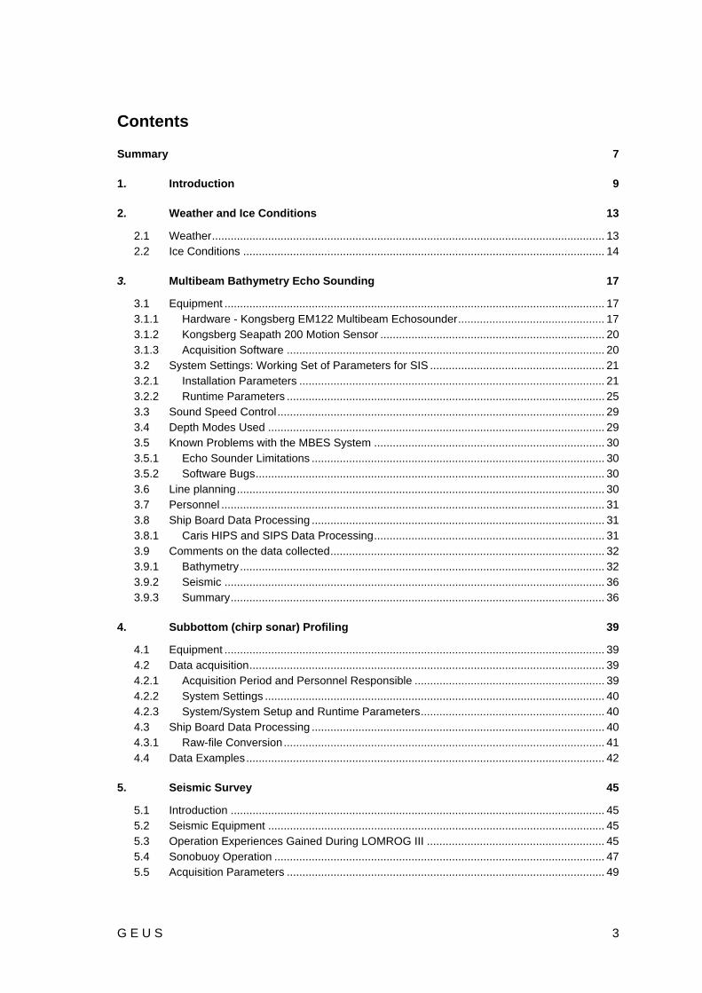
3.2.2.3 Filters and Gains

Figure 18. Runtime parameters – Filter and Gains

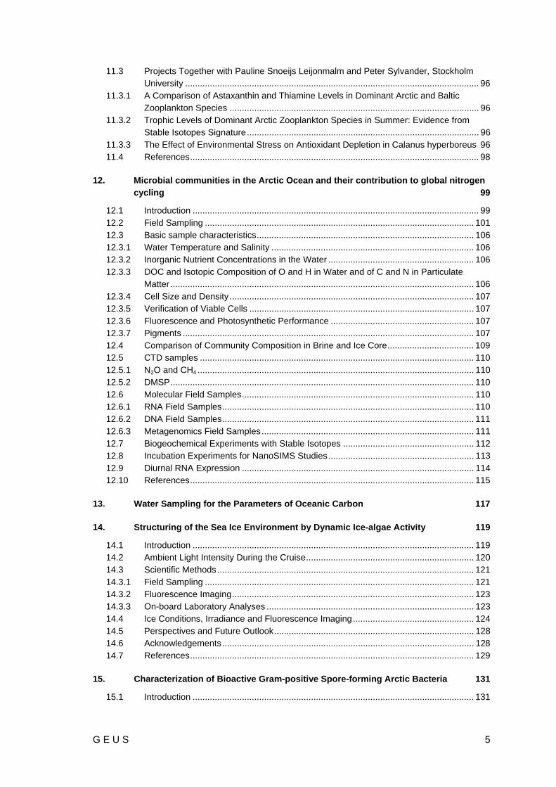
3.2.2.4 Data Cleaning

Figure 19. Runtime parameters – Data Cleaning

28 G E U S

3.2.2.5 GPS and Delayed Heave

Figure 20. Runtime parameters – GPS and Delayed Heave

3.2.2.6 Survey Information

Figure 21. Runtime parameters – Survey Information

G E U S 29

3.3 Sound Speed Control Every time a sound velocity profile (SVP) was obtained, either from a ship CTD or a CTD taken at an ice station, the data were checked by operators from the Danish Meteorological Institute (DMI). When any errors had been corrected the accepted data (profile) were copied to a common directory on the ship’s RAID system.

Figure 22. Sound velocity profiles The data were then sub-sampled using a Python script, that converted the original data to depths and corresponding sound velocity pairs (max 999 lines).

The SIS software however requires the profile to be extended to 12 km so this was also done at the same time (again using a Python script). It should be noted that the profiles were very stable and changed little over the duration of the survey.

The sound speed from the Valeport Mini SVS/T sensor was used for sound speed at the transducer at the beginning of the cruise. Because of some problems with the sensor showing the wrong value (or nothing at all), it was decided to enter a manual value into the multibeam acquisition software based on the converted values from the actual CTD profiles.

3.4 Depth Modes Used Below is a list of modes and the suggested depth range that they are designed to support. This is also the depth intervals used by the automatic mode selection.

30 G E U S

Shallow (< 350 m) Medium (350 m-1000 m) Deep (1000 m-9000 m) Very Deep (> 9000 m)

It should be noted that the ping mode was set to run automatically at all times.

3.5 Known Problems with the MBES System

3.5.1 Echo Sounder Limitations

Like on earlier expeditions the Kongsberg multibeam is prone to Erik’s horns. Generally during transit the maximum across track beam angle were set to ±40º

due to noise in the data. Furthermore a higher setting resulted in a lower ping rate.

3.5.2 Software Bugs

As reported on the LOMROG II and EAGER expeditions - when working in projection, COG - Projection rotation at present position = DTK (Desired Track) (western LON negative). This means that the DTK must be corrected for latitude in order to work with the auto pilot. This bug affects in the Helmsman displays and the COG arrow in the geographical window. How to reproduce this bug: Set geographic window to projection. Plan line at some high longitude. The Helmsman DTK will then show the line course offset by the longitude.

Probably related to the previous bug – still a problem: The ship heading arrow points into the wrong direction when working in a projection with True North not equal Map North. Even working in UTM projection it is offset depends on where the ship is presented on the screen.

Depth scale of water column display does not match the depth scale in the e.g. cross track display because the water column data is not SVP corrected. It would be very useful to have a function for “locking” the digitizing of the sea floor from within the water column display, as it is often possible to “see” the seafloor and it appears that no bottom detections are logged.

The display of detections in the Cross track/Beam intensity, Water column and Geographical windows are not always synchronized.

3.6 Line planning Whenever possible the transit lines were chosen to pass over any “interesting” features found on (or nearby) the route to the next area of interest. This was done in order to determine if there was an actual feature on the sea-floor or if the IBCAO (version 3.0) chart just had an artefact left in its model data.

G E U S 31

Some discrepancies with the newest version of the IBCAO chart were found (see Chapter 5 for further details).

3.7 Personnel MBES measurements were carried out continuously during the entire expedition, with a team of six people working according to the following watch scheme. Time Name Affiliation Log

sheet initials

0-4 and 12-16

Rezwan Mohammad

Stockholm University, Sweden RM

Francis Freire Stockholm University, Sweden FF

4-8 and 16-20 Morten Sølvsten

National Survey and Cadastre, Denmark

MS

Niki Andersen GEUS, Denmark NA

8-12 and 20-24 Richard Pedersen

National Survey and Cadastre, Denmark

RP

Nina Kirchner Stockholm University, Sweden NK

Table 2. Watch scheme for the multibeam crew.

The watch time was “Ship Time”, which was UTC +2 during the entire expedition. The data time used everywhere was UTC.

3.8 Ship Board Data Processing All ship board processing of echo sounding data was carried out using CARIS HIPS and SIPS (version 7.1, SP2). A log sheet was kept and filled out using an OpenOffice Calc spreadsheet in order to get an overview of the actions taken regarding the processing of the data.

For visualization and additional control of the bathymetric data (cleaned in CARIS), Fledermaus (version 7) from IVS 3D was used. The new data could be combined (and compared) with both data from previous expeditions and the IBCAO model data.

During the cruise an inventory of all collected data was built in an Intergraph GeoMedia Professional (version 6.1) geographical information system.

3.8.1 Caris HIPS and SIPS Data Processing

Data conversion: The echo sounder raw data, in ALL format, were converted into Caris HDCS data using the Caris HIPS and SIPS conversion wizard.

Apply tide: Zero tide was applied to all data.

32 G E U S

Compute TPU: The total propagated error was computed. The surface sound speed was assumed to be within ±5 m/s and sound speed profile were assumed to be within ±10 m/s, all other values were set to zero. See CARIS Vessel Configuration File (Appendix 2, section 19.2.3) for more settings.

Merge: The data were merged. This process assigns geographic positions to all soundings and reduces them for tide and any other specified corrections such as new sound velocity profile.

Create field sheet: Field sheets were generated to the most appropriate resolution based on depth. The cube surfaces varied between 50 m and 100 m. An overall field sheet with a 100 m cube surface was used for quality check.

Data cleaning and gridding: Manual data cleaning was performed throughout the survey using the subset editor (after data were merged). The data cleaning was done as an iterative process by different persons each time. Sometimes deciding about the quality of single soundings can be difficult given the sometimes bad data quality (especially during ice breaking).

Quality control, final field sheets and bathymetric grids: Fledermaus (version 7) was used on a daily basis for quality control and any spikes found using Fledermaus were then cleaned in CARIS – and hence a new surface was exported. The field sheets set up were used as both working sheets. The final layout was determined at the end of the cruise (see section 3.9.3).

3.9 Comments on the data collected

3.9.1 Bathymetry

In general, the profiles measured while crossing the Lomonosov Ridge match the latest IBCAO model (version 3) very well. However, at some locations some bathymetric highs are underestimated in the model.

G E U S 33

Figure 23. The main part of the bathymetric data collected during the LOMROG-III expedition

The detailed bathymetric mapping at the first crossing of the Lomonosov Ridge, marked as number 1 (in Figure 23), has shown that the ridge itself actually consists of several en echelon ridges. This conclusion is also supported by the adjacent single beam soundings.

Figure 24. Details of crossing 1. The front of this elevation shows a very steep slope towards the deep ocean seafloor. The shoalest depth measured were approximately 2445 m rising from the ocean seabed at 3850 m water depth. It may also be noted that the feature was not present in the IBCAO model. On the same location the IBCAO model shows a depression in the seafloor.

34 G E U S

The second crossing, marked as number 2 (in Figure 23), of the Lomonosov Ridge show (like the first crossing) what is believed to be the end of one of the en echelon ridge systems. The front of this elevation does not show quite as steep a slope towards the deep ocean seafloor as the first crossing. The shoalest depth measured were approximately 2700 m rising from the ocean seabed at 4000 m water depth. It may also be noted that the feature was present in the IBCAO model but not as high as measured on this expedition.

Figure 25. Details of crossing 2. The third crossing, marked as number 3 (in Figure 23), of the Lomonosov Ridge also show the same type of en echelon ridge system. The forefront of this elevation shows a steep slope towards the ocean seafloor (approx. 31º). The shoalest depth measured were approximately 2000 m rising from the ocean seabed at 4000 m water depth.

Figure 26. Details of crossing 3.

To the north of the shown profile it may be seen that the data does not match the IBCAO model. The new data is more pronounced than the model data indicates. It looks like the most northern point of en echelon ridge system is reached.

Mapping the area around the most eastern part of the Lomonosov Ridge (marked as no. 4 in Figure 23) it may be noted that the outcrop in the IBCAO model of the Lomonosov Ridge

G E U S 35

to the west does not exist. The FOS and BOS will therefore be moved to the east by approximately 13 km. The southernmost point on this part of the Lomonosov Ridge is consistent with the IBCAO model.

Figure 27. IBCAO model overlain with LOMROG-III multibeam data on the Lomonosov Ridge.

On the transit south, a small isolated elevation of a rounded shape (approx.400 m high) in the IBCAO model, was investigated to prove (or rather disprove) its existence. On the position a pirouette was carried out to get the best coverage in the area. The collected multibeam data show that the small feature does not exists on the location indicated in the model. Therefore it is advised to remove this feature from the current IBCAO model.

Figure 28.The small feature in the IBCAO model overlaid with LOMROG-III multibeam data.

36 G E U S

3.9.2 Seismic

Seismic data acquisition was planned during the third crossing of the Lomonosov Ridge. Due to difficult ice conditions with an unfortunately high drift, multibeam data acquired on this crossing are sparse.

For each seismic line Oden first had to break a lead twice in order to be able to acquire seismic data along a pre-planned line without a risk for damage or loss of equipment. Under normal drift conditions the planned seismic line would therefore be surveyed with the multibeam system three times resulting in reasonably good (and dense) data.

Figure 29. Details of crossing 3 – multibeam data acquired along the seismic line.

Multibeam data collected during passage along all the seismic lines were supplied daily to the seismic team in order to facilitate proper geometry in seismic processing.

3.9.3 Summary

During LOMROG-III Oden travelled a total of 3.672 nautical miles. Multibeam data were acquired during the entire cruise.

A total of 10 final field sheets were created in Caris covering all data collected during the LOMROG-III expedition (Figure 30):

3 field sheets in the Amundsen Basin

2 field sheets on the Lomonosov Ridge

5 field sheets for the transit to/from Longyearbyen and between areas mentioned above.

It should be noted that the bathymetric data acquired during the LOMROG-III cruise will be incorporated in the IBCAO database.

G E U S 37

Figure 30. Regional map showing all field sheets created during the LOMROG-III cruise.

38 G E U S


G E U S 39

4. Subbottom (chirp sonar) Profiling

By Nina Kirchner & Richard Gyllencreutz, Stockholm University

4.1 Equipment The icebreaker Oden is equipped with a Kongsberg SBP120 3ºx 3º subbottom profiler primarily used for the acoustic imaging of the topmost sediment layers beneath the sea floor. The SBP120 subbottom profiler is an add-on to the EM122 multibeam echo sounder installed on Oden, and operates at a frequency range of 2.5-7 kHz. It uses an extra transducer array, whereas one single broadband receiver transducer is used for the EM 122 multibeam echo sounder and the SBP120 system. A frequency splitter directly after the receiver staves separates the ~12 kHz multibeam signal from the lower-frequency chirp sonar signal.

The normal transmit waveform is a chirp signal in the form of a frequency modulated (FM) pulse, either swept linearly or hyperbolically. Beyond these standard FM pulse forms, the SBP120 provides a number of additional pulse forms (non-chirp signals) to choose from (for a description of those, cf. Kongsberg SBP120 operator manual). Chirp signals have a vertical resolution roughly given by the inverse of the sweep range (difference between sweep high frequency fH and sweep low frequency fL ). With fH= 7 kHz and fL = 2.5 kHz, the system provides a maximal vertical resolution of approximately 1/ 4.5 milliseconds (ms) = 0.3 ms.

The SBP120 is capable of providing beam opening angles down to 3º, and up to 11 beams in a transect across the ship's keel direction with a spacing of usually 3º. The system is fully compensated for roll, pitch and heave movements of the ship by means of the Seatex Seapath 200 motion sensor used for the multibeam echo sounder.

4.2 Data acquisition

4.2.1 Acquisition Period and Personnel Responsible

The SBP120 chirp sonar was continuously operated during the entire cruise from 20120731-20120913 (45 days), with occasional pauses in logging, e.g. during coring. A handwritten log (updated by the operators on watch) was used to document as accurately as possible any logging pauses, problems encountered in connection with the multibeam- and chirp sonar data acquisition, or temporary changes made in system settings. Data acquisition was performed by the multibeam technicians (Table 2), and using UTC time throughout as data time.

40 G E U S

4.2.2 System Settings

The general settings for the SBP120 system are loaded via the configuration file. Due to initial problems with the NMEA readers, different versions of the configuration file were used in the beginning of the cruise. After the initial complications were resolved, the system ran stable with the settings provided in the file SBPConfig_LOMROG3_120811_SERIAL_POS.xml. For convenience, this file is archived along with all acquired chirp data. When in use, the path to the config.file is C:\Program Files\Kongsberg Maritime\KM SBP OPU\.

The subdirectories C:\Program Files\Kongsberg Maritime\KM SBP OPU\config_files\ and C:\Program Files\Kongsberg Maritime\KM SBP OPU\Old Config files\ contain earlier, but no longer used, versions of the configuration file.

4.2.3 System/System Setup and Runtime Parameters

The following specific system settings were used as defaults for the SBP120 during the cruise:

Transmit mode: Normal Synchronisation: EM trigger Acquisition delay: Depending on water depth as received from the multibeam echo sounder;

between 1000 milliseconds (ms) and 6000 ms Acquisition window: 300 ms. Note that there is a bug in the SBP120 since the true acquisition

window is always 100 ms larger than the specified one. With the default setting of 300 ms, data was thus acquired in a 400 ms window.

Reduce Em <> SBP crosstalk: ticked on Pulse form: Hyperbolic chirp up (best trade-off of energy/penetration and resolution) Sweep frequencies: 2500 Hz (low), 7000Hz (high) Minimize pulse shape: ticked off Pulse shape: 10% Pulse length: 100 ms Source power: 0dB (always needs to be set to this manually after start-up) Beam width Tx/Rx: Normal Number of beams: 5 Beam spacing: 3º Calculate delay from depth: ticked off Automatic slope correction: ticked off Slope along/across: 0.0 Slope quality: 0.0

4.3 Ship Board Data Processing All shipboard processing of the chirp sonar data was carried out by Nina Kirchner and Richard Gyllencreutz using the Kongsberg SBP120 software version 1.4.6.

The SBP120 raw-files were screened during a replay in the SBP120 software. For replaying and subsequent conversion of the raw-files into jpg-files, the configuration file SBP120Config_DataProcessing_NKRG_LOMROG2012.xml was used. A documentation of which raw-files were/were not converted into jpg-files, and from how many raw-files an

G E U S 41

individual jpg-file is made, is given in the processing log file README_LOMROG12_SBP.txt. For easy reference, both files are archived together with the raw-data. The jpg-files are stored using the same per-day structure as the raw-files. Further post-processing of the data could not be performed during the cruise. SBP profiles at or as close as possible to the coring sites, are shown in section 4.3 for the sites where good quality data was obtained.

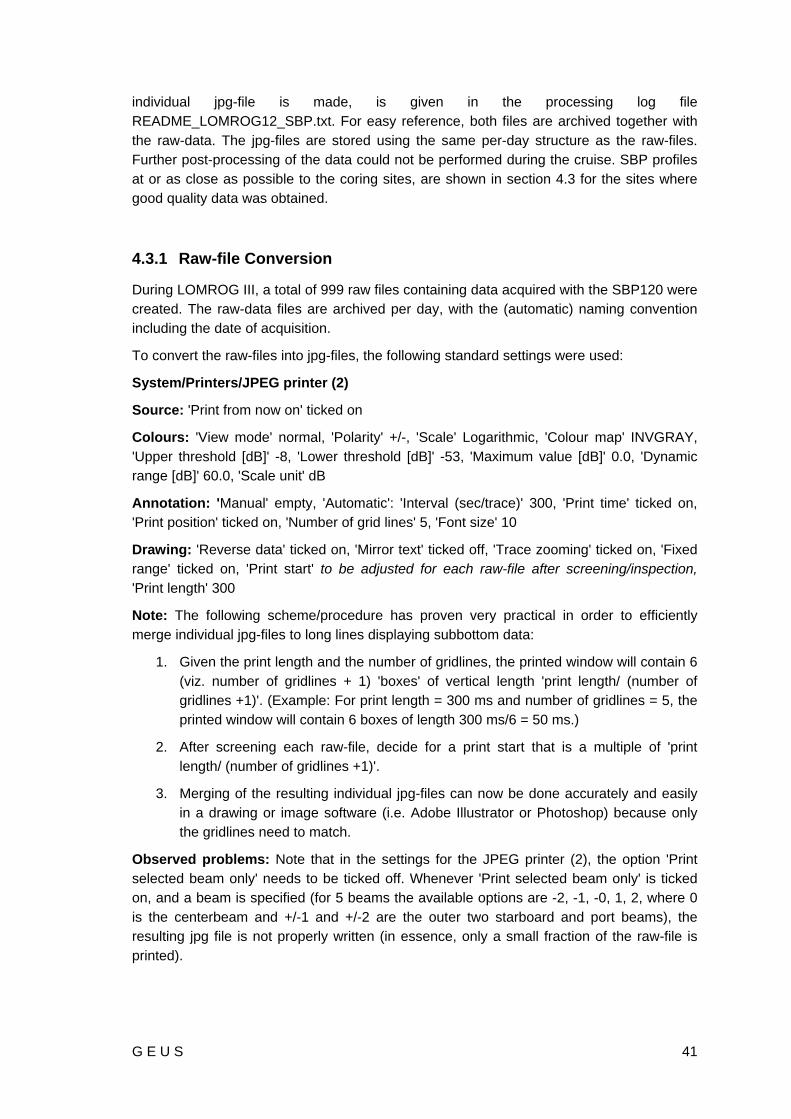
4.3.1 Raw-file Conversion

During LOMROG III, a total of 999 raw files containing data acquired with the SBP120 were created. The raw-data files are archived per day, with the (automatic) naming convention including the date of acquisition.

To convert the raw-files into jpg-files, the following standard settings were used:

System/Printers/JPEG printer (2)

Source: 'Print from now on' ticked on

Colours: 'View mode' normal, 'Polarity' +/-, 'Scale' Logarithmic, 'Colour map' INVGRAY, 'Upper threshold [dB]' -8, 'Lower threshold [dB]' -53, 'Maximum value [dB]' 0.0, 'Dynamic range [dB]' 60.0, 'Scale unit' dB

Annotation: 'Manual' empty, 'Automatic': 'Interval (sec/trace)' 300, 'Print time' ticked on, 'Print position' ticked on, 'Number of grid lines' 5, 'Font size' 10

Drawing: 'Reverse data' ticked on, 'Mirror text' ticked off, 'Trace zooming' ticked on, 'Fixed range' ticked on, 'Print start' to be adjusted for each raw-file after screening/inspection, 'Print length' 300

Note: The following scheme/procedure has proven very practical in order to efficiently merge individual jpg-files to long lines displaying subbottom data:

1. Given the print length and the number of gridlines, the printed window will contain 6 (viz. number of gridlines + 1) 'boxes' of vertical length 'print length/ (number of gridlines +1)'. (Example: For print length = 300 ms and number of gridlines = 5, the printed window will contain 6 boxes of length 300 ms/6 = 50 ms.)

2. After screening each raw-file, decide for a print start that is a multiple of 'print length/ (number of gridlines +1)'.

3. Merging of the resulting individual jpg-files can now be done accurately and easily in a drawing or image software (i.e. Adobe Illustrator or Photoshop) because only the gridlines need to match.

Observed problems: Note that in the settings for the JPEG printer (2), the option 'Print selected beam only' needs to be ticked off. Whenever 'Print selected beam only' is ticked on, and a beam is specified (for 5 beams the available options are -2, -1, -0, 1, 2, where 0 is the centerbeam and +/-1 and +/-2 are the outer two starboard and port beams), the resulting jpg file is not properly written (in essence, only a small fraction of the raw-file is printed).

42 G E U S

Systematic tests using different raw-files and different beams all resulted in truncated jpg-files when 'Print selected beam only' was ticked, but with correct result if ticked off.

4.4 Data Examples

Figure 31a. SBP profile near coring site PC03

b. SBP profiles near coring sites TC04 - PC05

Figure 32a. SBP profiles near coring site PC07 b. SBP profiles near coring site PC08

G E U S 43

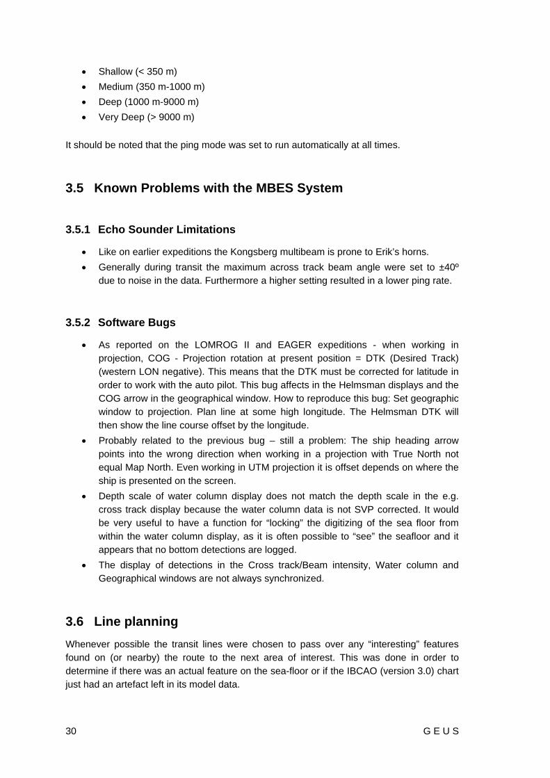
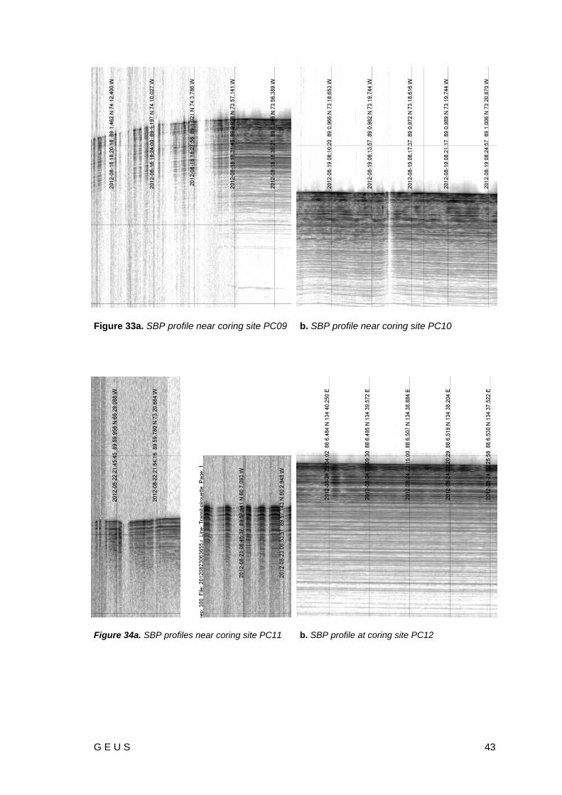
Figure 33a. SBP profile near coring site PC09

b. SBP profile near coring site PC10

Figure 34a. SBP profiles near coring site PC11

b. SBP profile at coring site PC12

44 G E U S


G E U S 45

5. Seismic Survey

By Thomas Varming, Bureau of Minerals and Petroleum; Per Trinhammer, University of Aarhus; Thomas Funck, John Hopper & Christian Marcussen, Geological Survey of Denmark and Greenland( GEUS)

5.1 Introduction Acquisition of seismic data in the Amundsen Basin and on the Eastern flanks of the Lomonosov Ridge was the second priorities of the LOMROG III cruise. A comprehensive Seismic Acquisition Report has been prepared separately (Varming et al, 2012). The following is a short account on some of the experiences and results gained during the LOMROG III cruise regarding acquisition of seismic data in ice filled waters.

5.2 Seismic Equipment Harsh environmental conditions in the Arctic have played a crucial role in the design of the seismic equipment and the modifications done to the setup. These modifications were made in cooperation with the Department of Earth Science at the University of Aarhus, based on previous experiences with seismic data acquisition in ice-filled waters and the two previous LOMROG expeditions in 2007 and 2009.

The use of a short streamer section of 200 m and a seismic source considerably smaller than what is often used in open water is some of the key elements of the seismic system. Another important element is the use of only one cable, trough the umbilical, onto which both the streamer and the airgun is attached making deployment and recovery simple. Both the gun and the streamer are towed at 20 m, typically twice the depth as for surveys in open water.

Compared to the previous cruise a larger airgun array is used consisting of two 520 cu. inch Sercel G-gun in order to increase the penetration of the seismic array.

5.3 Operation Experiences Gained During LOMROG III The operative experiences gained during the first two LOMROG expeditions were the basis for the deployment of the seismic equipment on the LOMROG III cruise, but in addition, two new improvements in the deployment phase have been implemented.

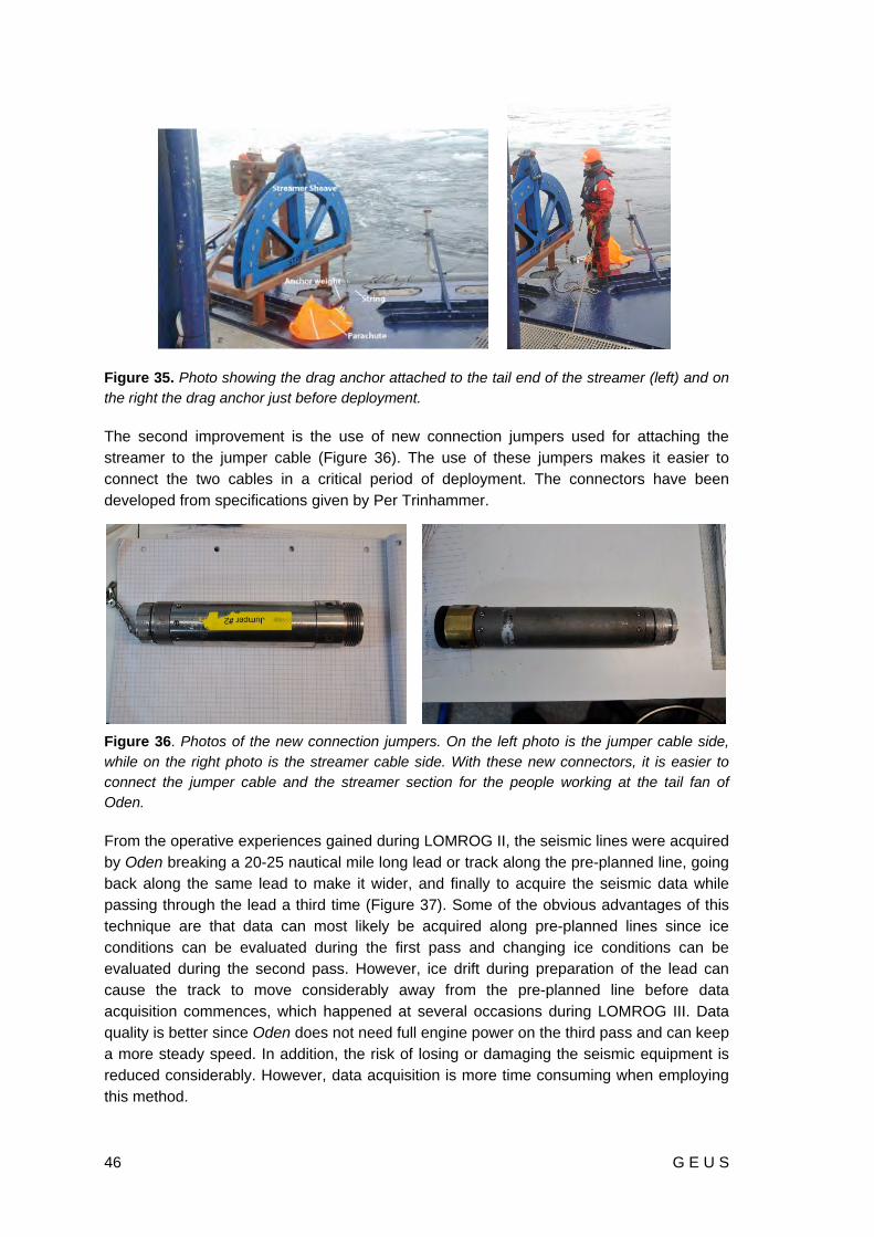
The first is the use of a drag anchor (Figure 35) attached to the end of the streamer acts as an efficient weight in the deployment of the streamer, keeping the streamer at a near vertical position during the deployment. While Oden increases its speed, the drag of the drag anchor exceeds the breakage point of the strings attached and the anchor sinks to the bottom, while the streamer raises itself in the water column.

46 G E U S

Figure 35. Photo showing the drag anchor attached to the tail end of the streamer (left) and on the right the drag anchor just before deployment.

The second improvement is the use of new connection jumpers used for attaching the streamer to the jumper cable (Figure 36). The use of these jumpers makes it easier to connect the two cables in a critical period of deployment. The connectors have been developed from specifications given by Per Trinhammer.

Figure 36. Photos of the new connection jumpers. On the left photo is the jumper cable side, while on the right photo is the streamer cable side. With these new connectors, it is easier to connect the jumper cable and the streamer section for the people working at the tail fan of Oden.

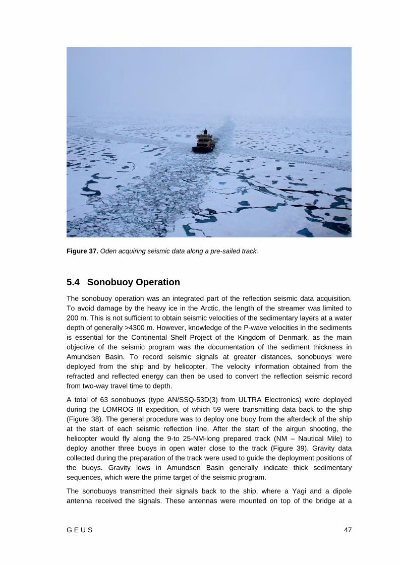
From the operative experiences gained during LOMROG II, the seismic lines were acquired by Oden breaking a 20-25 nautical mile long lead or track along the pre-planned line, going back along the same lead to make it wider, and finally to acquire the seismic data while passing through the lead a third time (Figure 37). Some of the obvious advantages of this technique are that data can most likely be acquired along pre-planned lines since ice conditions can be evaluated during the first pass and changing ice conditions can be evaluated during the second pass. However, ice drift during preparation of the lead can cause the track to move considerably away from the pre-planned line before data acquisition commences, which happened at several occasions during LOMROG III. Data quality is better since Oden does not need full engine power on the third pass and can keep a more steady speed. In addition, the risk of losing or damaging the seismic equipment is reduced considerably. However, data acquisition is more time consuming when employing this method.

G E U S 47

Figure 37. Oden acquiring seismic data along a pre-sailed track.

5.4 Sonobuoy Operation The sonobuoy operation was an integrated part of the reflection seismic data acquisition. To avoid damage by the heavy ice in the Arctic, the length of the streamer was limited to 200 m. This is not sufficient to obtain seismic velocities of the sedimentary layers at a water depth of generally >4300 m. However, knowledge of the P-wave velocities in the sediments is essential for the Continental Shelf Project of the Kingdom of Denmark, as the main objective of the seismic program was the documentation of the sediment thickness in Amundsen Basin. To record seismic signals at greater distances, sonobuoys were deployed from the ship and by helicopter. The velocity information obtained from the refracted and reflected energy can then be used to convert the reflection seismic record from two-way travel time to depth.

A total of 63 sonobuoys (type AN/SSQ-53D(3) from ULTRA Electronics) were deployed during the LOMROG III expedition, of which 59 were transmitting data back to the ship (Figure 38). The general procedure was to deploy one buoy from the afterdeck of the ship at the start of each seismic reflection line. After the start of the airgun shooting, the helicopter would fly along the 9-to 25-NM-long prepared track (NM – Nautical Mile) to deploy another three buoys in open water close to the track (Figure 39). Gravity data collected during the preparation of the track were used to guide the deployment positions of the buoys. Gravity lows in Amundsen Basin generally indicate thick sedimentary sequences, which were the prime target of the seismic program.

The sonobuoys transmitted their signals back to the ship, where a Yagi and a dipole antenna received the signals. These antennas were mounted on top of the bridge at a

48 G E U S

height of 27-29 m above sea level. Data were then recorded by a Taurus seismometer and on the auxiliary channels of the seismic recording system (Geometrics). With the Yagi antenna, seismic signals could be recognized up to a distance of 34 km from the ship, the dipole antenna generally worked in ranges up to 18 to 24 km. To determine the exact distance to the drifting sonobuoys, the travel time of the direct water wave was modelled with the water velocity function obtained from the onboard CTD measurements.

The overall quality of the data is excellent and will allow for a high-resolution definition of the velocities within the sedimentary column employing semblance analysis or more sophisticated two-dimensional ray tracing methods. In addition, many records show crustal refractions and sometimes even reflections from the Moho discontinuity. Since the setup of most lines was similar to classic wide-angle seismic reflection/refraction experiments, the crustal velocity structure beneath the Amundsen Basin and the flank of the Lomonosov Ridge can be determined.

Figure 38. Bathymetric map (IBCAO 3.0) with the location of the LOMROG III (2012) seismic reflection lines (red lines). White circles indicate the deployment positions of the 59 sonobuoys that transmitted seismic data.

G E U S 49

Figure 39. Deployment of sonobuoy in open water close to the prepared track for the seismic line (left). After activation by salt water, an orange buoy inflates, which holds the antenna that transmits the hydrophone signals to the ship (right).

5.5 Acquisition Parameters

Table 3. Summary of acquisition parameters

Source 2*Sercel G-Gun Chamber volume 2*520 cu. inch Gun pressure 180 bar (2600 psi) Mechanical delay Automatically adjusted to 0 ms Nominal tow depth 20 m Streamer Geometrics GeoEel Length of tow cable 30 m Length of stretch section 53 m No of active sections 4 Length of active sections 200 m No of groups in each section 8 Total no of groups 32 Group interval 6.25 m No of hydrophones in each group 8 Depth sensors in each section Nominal tow depth 20 m Acquisition system Geometrics GeoEel controller Sample rate 1 ms Low-cut filter Out High-cut filter Anti-alias (405 Hz) Gain setting 0 dB No of recording channels 32 No of auxiliary channels 8 Shot interval 14 s ± 1 s Record length 12 s

50 G E U S

5.6 Processing Parameters Processing the seismic reflection data collected during LOMROG III follows the procedures developed during LOMROG II in 2009 (Hopper and Marcussen, 2010) and EAGER (Marcussen et al., 2012). The computer setup and details are identical to EAGER except that the Linux Centos 4.7 virtual machine was ported from Parallels to VMWare Fusion. The scripts and processing flows from the previous cruises were used with only small modifications. See Appendix C of the LOMROG II processing report for the key scripts (Hopper and Marcussen, 2010). The basic processing was done in ProMAX 2003.19.1.

In the LOMROG II processing report it was mentioned that some of the techniques recommended in Jokat et al. (1995) should be tried on the LOMROG data sets. Jokat et al. noted that a key problem with processing data collected in the Arctic is that noise, in particular noise from ice hitting the equipment, is especially difficult to eliminate. They addressed this by using a median stack. Median stacking suppresses noise by giving less weight to outlier amplitudes associated with random bursts of energy. To work effectively, the mid-point bin size should be sufficiently large to ensure good data fold and sampling statistics.

The natural bin size for a streamer with 6.25 m group interval is 3.125 m. The average data fold for the LOMROG and EAGER cruises is around 4 with this bin size (shooting interval of 25-30 m and 32 active channels). During LOMROG II and EAGER, tests on increasing the bin size to give higher fold had only minimal impact on the imaging quality using simple averaging for producing the stack. In part, this is because trace mixing and combining CDP's for plotting and display has the net effect of increasing the fold to the same as would be achieved with a 12.5 or 25 meter bin. Because the results of this could be quite different for median stacking, some tests were run on this cruise by assigning geometry with 12.5 and 25 meter bins. The data were stacked with both median and mean methods and no significant difference between the stacks was found. Therefore the median stacking method was not used and the binning and processing flow here follows that of the previous cruises.

For all seismic reflection lines on this cruise, the ice adapted towing arrangement was used. The seismic source consisted of two 520 cu. in. G-Guns roughly double the volume used in 2009. The larger array easily penetrated to basement in all areas surveyed. In some cases, reflections below basement may be indicated. Depth transducers were initially placed at the near end of each section. Prior to shooting Line 4, the depth transducer of the far section was moved to the far end of the streamer. During Line 10 acquisition, the streamer developed leakage problems and was replaced with the spare sections. During this change, depth transducers were again placed at the beginning of each section (beginning with Line 10D). Shots were fired on randomised time and auxiliary channels were used to record the sonobuoys.

The basic processing sequence is as follows:

1. SEG-D read with trace dc bias removal; 2. Bandpass filter; 3. User defined spectral shaping filter; 4. Spike and noise burst editing; 5. Shot gather f-k filter and resample to 2 ms. 6. Geometry assignment, including gun and cable statics;

G E U S 51

7. Trace equalization; 8. Velocity Analysis (Lines 5 and 6 only) 9. Trace mixing on shot gathers; 10. Midpoint sort and stack; 11. Final geometry and amplitude recovery; 12. Post-stack constant velocity migrations; 13. Seafloor mute; 14. SEG-Y output; 15. grd conversion and plot.

5.7 Results Planning of the seismic lines in the Amundsen Basin was based on available data, primarily compilations of the LOMGRAV 2009 gravity data and older seismic data. The purpose of these lines was to map the sediment thickness and therefor gravity minima were investigated.

During the LOMROG III cruise a total of 497.5 km of seismic data were acquired, with no loss of equipment during the cruise. However, there was one incidence where the airgun array was hit by an ice floe causing damage to the cabling of the airgun (Figure 40). Repair was done within a couple hours. Due to severe ice-conditions data acquisition had to be terminated twice on the Lomonosov Ridge despite a lead had been prepared.

Figure 40. Photos of the damage done to the airgun array from hitting an ice floe. Note the piece of ice still stuck to left side of the airgun array.

52 G E U S

5.8 Staffing

The seismic operations were carried out by ten members of the scientific crew on-board Oden as listed in Table 4.

Name Affiliation Function

Thomas Funck GEUS Geophysicist in charge of sonobuoy operations

John R. Hopper GEUS Processing geophysicist

Thomas Varming BMP Geophysicist

Per Trinhammer Aarhus University Chief technician

Simon Ejlertsen Aarhus University Technician

Lars Georg Rödel GEUS Technician

Jack Schilling NIOZ Technician

Trine Kvist-Lassen GEUS, Aarhus University Watch keeper and deck hand

Marie Lykke Rasmussen GEUS, Aarhus University Watch keeper and deck hand

Sofie Ugelvig GEUS, Aarhus University Watch keeper and deck hand

Table 4. Staffing of the seismic operation during LOMROG III

5.9 References Hopper, J. R. & Marcussen, C. 2010: Seismic Processing Report – LOMROG II in 2009.

Acquisition of reflection and refraction seismic data during Oden’s Lomonosov Ridge Off Greenland (LOMROG II) cruise in 2009. Danmarks og Grønlands Geologiske Undersøgelse Rapport 2010/36, 99 pp. + 3 DVD’s (confidential).

Jokat, W., Buravtsev, V. Y. & Miller, H. 1995: Marine seismic profiling in ice covered regions. Polarforschung 64 (1), 9-17.

Varming, T., Funck, T., Hopper, J. R., Trinhammer, P., Ejlertsen; S., Rödel, R., Schilling, J., Kvist-Lassen, T., Rasmussen, M. L., Ugelvig, S. & Marcussen, C. 2012: Seismic Acquisition Report – LOMROG III in 2012. Danmarks og Grønlands Geologiske Undersøgelse Rapport 2012/120, 77 pp. + 5 Appendices + 1 DVD.

G E U S 53

6. Single beam Bathymetry Echo Sounding

By Morten Sølvsten and Richard Pedersen, National Survey and Cadastre Bathymetric spot soundings have been collected to supplement the multibeam data acquisition. This was done in combination with the acquisition of gravimetric data at the same locations.

6.1 Equipment The equipment used during LOMROG III was the same as used on earlier expeditions with good results. A modified Reson Navisound 420-DS echo sounder (serial no. 97037) was mounted in a flight case and installed in the helicopter. The echo sounder was controlled by a GETAC M220-5C21 ruggedized notebook using the Reson NaviSound Control Center software (which also logged the digital data). The echo sounder’s paper trace was enabled and annotated as a backup/supplement to the digital data. The echo sounder used an Airmar M175 (12kHz-C) transducer that had been fitted with handles. Positioning was done by connecting a battery powered Thales Mobile Mapper stand-alone GPS receiver (hand-held) to the echo sounder. The helicopter provided 28V DC to the echo sounder.

6.2 Results The single beam team consisted of Morten Sølvsten and Niki Andersen. The team was deployed by the ship’s helicopter to pre-planned positions well outside of Oden’s multibeam coverage. The lines were typically planned to be approximately 9 nautical miles distance from the ship’s track. With a five kilometre interval between soundings, 4 profiles of the up-/down slope of the Lomonosov Ridge were made (Figure 41). These profiles were made parallel to the ship’s track. Figure 41. The four single beam lines collected by helicopter.

54 G E U S

The positions were chosen such that the depths acquired would include the 2500 metre contour and the FOS (Foot of Slope) location. Line_01: The measured depths correlate well with the IBCAO model. It may be noted that the inner part of the slope is measured to be steeper and closer to the Amundsen Basin.

Figure 42. Single beam Line_01. Depths are plotted at the 5 kilometre interval as the depths were observed. The IBCAO Version 3.0 grid data are shown for comparison. Line_01a: The measured depths correlate well with the IBCAO model. It may be seen that a small depression in the seafloor shows up close to the Amundsen Basin.

Figure 43. Single beam Line_01a. Depths are plotted at the 5 kilometre interval as the depths were observed. The IBCAO Version 3.0 grid data are shown for comparison.

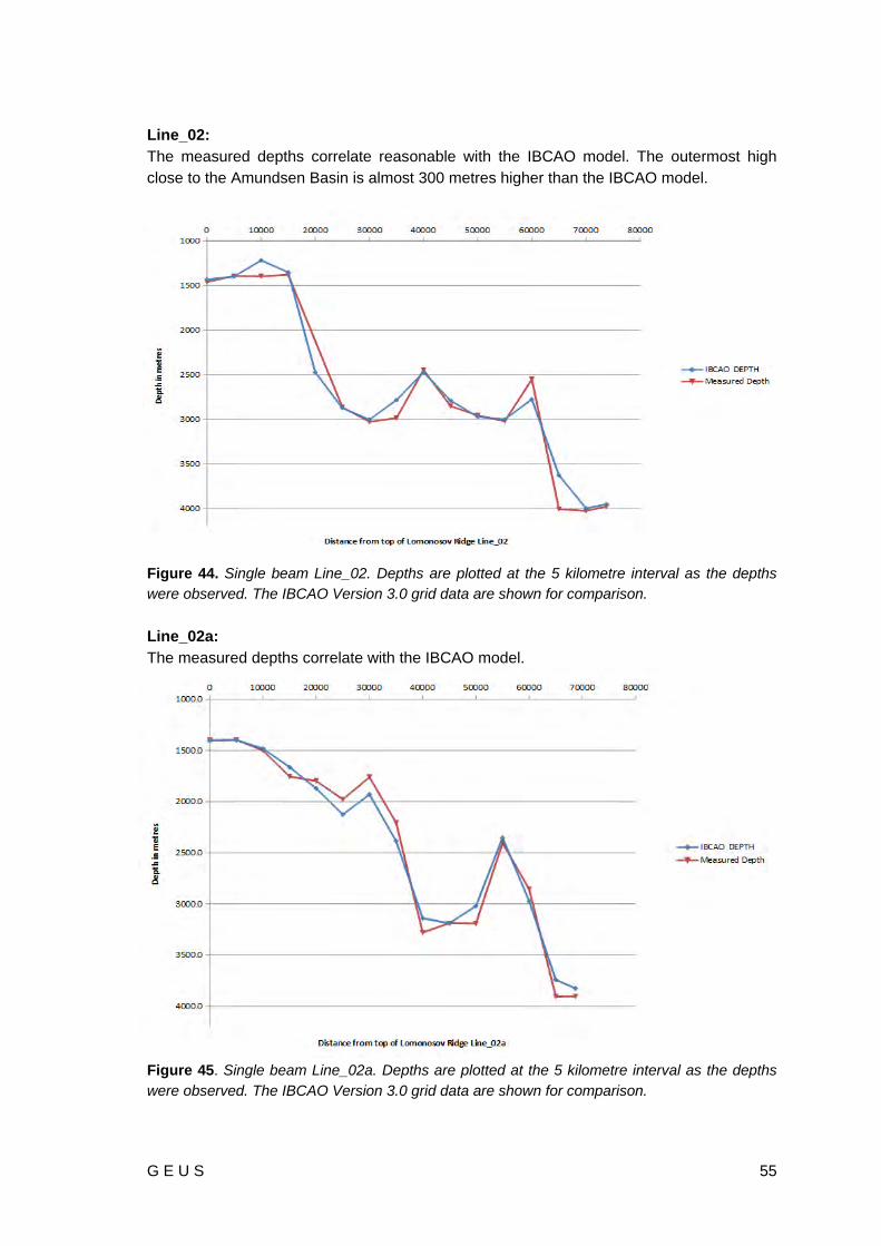
G E U S 55

Line_02: The measured depths correlate reasonable with the IBCAO model. The outermost high close to the Amundsen Basin is almost 300 metres higher than the IBCAO model.

Figure 44. Single beam Line_02. Depths are plotted at the 5 kilometre interval as the depths were observed. The IBCAO Version 3.0 grid data are shown for comparison. Line_02a: The measured depths correlate with the IBCAO model.

Figure 45. Single beam Line_02a. Depths are plotted at the 5 kilometre interval as the depths were observed. The IBCAO Version 3.0 grid data are shown for comparison.

56 G E U S

The bathymetry data were acquired at a fixed average sound speed of 1500 m/s and the field values were later corrected (during post-processing) using the appropriate average sound speed at the given depth based on CTD casts made from either Oden or station on the sea ice.

A zero tide value was applied (as it was done with all of the multi-beam data). Hand written notes were also made in the field at each sounding position. This documentation will be used as part of the quality control and include position, time and registered depth.

During the LOMROG-III expedition a total of 69 successful singlebeam soundings were made ranging from 1172 meters to 4024 meters.

At all the sounding positions gravity measurements were simultaneously acquired by Indriði Einarsson from DTU Space.

An ice-dampened Lacoste & Romberg land gravimeter (serial no. G932) was used for the gravity measurements. This set-up had proved its durability during previous expeditions in temperatures down to minus 40ºC.

Below a comparison is shown between the corrected bathymetry and the measured gravity done by Indriði Einarsson for each profile.

Figure 46. Comparison between bathymetry and gravity data along line 1.

G E U S 57

Figure 47. Comparison between bathymetry and gravity data along line 1a.

Figure 48. Comparison between bathymetry and gravity data along line 2.

58 G E U S

Figure 49. Comparison between bathymetry and gravity data along line 2a.

G E U S 59

7. Gravity Measurements during LOMROG III

By Indriði Einarsson, National Space Institute (DTU Space)

7.1 Introduction Marine gravity data reflect the bathymetry and the density distribution of the oceanic crust and mantle. Low gravity values are related to low densities, submarine canyons, and trenches at the bottom of the sea. High gravity values are related to high densities, seamounts, and ocean ridges. Gravity increases generally towards the poles due to the flattening and rotation of the earth. After removal of this effect, gravity anomalies can be identified. Variations in gravity anomalies are expressed in mGal (1 mGal = 10-5 m/s2), and a 1mGal change in gravity corresponds roughly to 7 meters bathymetry in the “free air anomalies”.

Coincident measurements of gravity and water depth makes it possible to compute so called Bouguer anomalies. Thereby, the gravity effect of the bathymetry is calculated and removed from the measured gravity values, under the assumption of constant density. This makes it possible to remove the bathymetric contribution from the gravity signal, and isolate the non-bathymetric signal, which indicates density variations below the seabed. This can be used as an aid in estimation of sediment thickness.

During the LOMROG III cruise the gravity acceleration has been measured by staff from the National Space Institute (DTU Space). Coincident high resolution observations of the bathymetry obtained from multi- and single beam sounders (see Chapter 3 and 6) give the unique opportunity to support the interpretation of seismic data. Further, the data can be used to improve existing gravity models of the Arctic Ocean, i.e. the Arctic Gravity Project (ArcGP).

7.2 Equipment A marine gravimeter, an Ultrasys LaCoste and Romberg (serial no.: S-38) was installed in the pump room near the centre-of-mass of the ship (the same location as during LOMROG I and II) to minimize the effect of the ship’s movement (Figure 50).

The instrument is in principle an ultra-precise spring balance with a “proof mass”, which is mounted on a gyro-stabilized platform. Levelling is maintained by a sophisticated feedback mechanism. The accuracy of the marine gravimeter is about 1 mGal with 200-500 m horizontal resolution in the final map. This variation is however dependent on ice conditions and the speed of the Oden.

60 G E U S

Figure 50. Ultrasy S38 marine gravimeter mounted in Oden’s pump room.

To complement the marine gravity measurements, measurements were made on the ice using a helicopter. For this phase of the program, a LaCoste and Romberg relative gravimeter (serial no.: G-867) owned by DTU Space was used (Figure 51). This gravimeter has the option to operate in a dampened mode. This is especially suited for measurements on sea-ice, where wave movements make the use of traditional, undampened land-gravimeters impossible. The estimated relative accuracy of the measurements is 0.2 mGal under average conditions. On few occasions, the accuracy was reduced by strong movement of the ice or by ice-floes colliding into each other. This will be documented in more detail in the detailed gravity acquisition and processing report.

G E U S 61

Figure 51. LaCoste Romberg G867 damped land gravimeter

7.3 Measurements The marine gravimeter operated in “marine mode” during the entire cruise and logged data every 10 seconds along Oden’s entire track. In addition, a total of 77 gravity readings were measured on the ice.

Of the 77 gravity measurements, 69 were measured along 4 lines parallel to the ship track across the Lomonosov Ridge (Figure 52). The distance between successive measurements along a line is 5 km. At each location the depth was measured using a single beam sounder (see Chapter 6). Each such measurement takes 5-10 minutes under ideal conditions.

The other 8 readings were done along Oden’s route, as close to Oden as possible: two by helicopter, the others by use of one of Oden’s cranes. Water depth measurements were not taken at these locations, since they serve the sole purpose of comparing the gravity readings of S-38 and G-867 and tying the ice-measurements to the S38-measurements.

62 G E U S

Figure 52. Oden’s track, measured gravity points (coloured) and control-points (red).

7.4 Ties Both the S-38 and G-867 are relative gravimeters. Therefore, they do not give absolute gravity values but only relative differences between measurement points. Most importantly, both instruments are subject to drift of the measured value, which for the timeframe of the LOMROG III cruise may be assumed to be linear with time. In order to correct for drift, the gravity readings of both the gravimeters need to be tied to known gravity values before and after the cruise. In order to calculate absolute gravity values from the relative measurements, a tie to the International absolute reference system is necessary. Such gravity reference points can be found in Longyearbyen, but unfortunately Oden was not able to dock at the beginning of the cruise and is not expected to do so at the end of the cruise either. Therefore, only the G-867 instrument could be tied to a reference point, while alternative methods have to be used to obtain a tie for the S-38 marine instrument. This has been done by taking a reading at Oden’s anchor position at Adventfjorden just off Longyearbyen, and comparing this to results of previous cruises, where a proper port tie was possible. This has been proven to give satisfactory results for the LOMROG II cruise.

G E U S 63

7.5 Processing At time of writing, preliminary data processing has been done by using the G-867 gravity reading at the gravity reference point in Longyearbyen as well as the reference gravity value in Longyearbyen fjord for the S-38 instrument. Since the gravity tie at the end of the cruise is yet to be done, no drift corrections can be made at this point. However, the preliminary results should give a good idea on the gravity field in this area. The positions of Oden were logged every 5 seconds with a Javad high precision dual frequency geodetic GPS receiver, which was mounted on top of a container on top of the bridge. This system serves as a backup system for Oden’s own GPS system, which provides positions on 10 seconds intervals. Once the gravity values are calculated, the gravity changes related to changes in bathymetry can be removed by using coincident data obtained from the single- or multibeam soundings. The remaining gravity signal originates from the different geological compositions below the sea bed, and is left for later interpretation to support the seismic work.

In cooperation with Thomas Funck and Morten Sølvsten, an experimental ad-hoc processing of gravity and bathymetric data was initiated in order to support the seismic measurements. While Oden prepared the lead in the ice for the seismic line (see Chapter 5), gravity, GPS and bathymetric data is acquired. When the lead has been prepared, Oden heads back to the start of the line, before seismic acquisition starts. Immediately after heading back, the gravity data are processed to gravity anomalies. Subsequently, the gravity anomalies can be used to obtain information on structures below the seabed, most importantly to locate possible sediment basins. This information is of use for refraction seismic measurements where sonobuoys are deployed, since those are preferably positioned above thick sediment layers. Since the gravity information is the only information on sediment highs and lows prior to seismic measurements, they have proven to be a useful help in positioning the sonobuoys, which are deployed by helicopter or ship prior to seismic measurements.

64 G E U S


G E U S 65

8. Sediment Coring

By Richard Gyllencreutz, Ludwig Löwemark, Jerker Eriksson & Nina Kirchner, Stockholm University

8.1 Introduction The project “PAWS: Palaeoceanography of the Arctic - Water masses, Sea ice, and Sediments” focuses on the critical role of the Arctic in the global climate system from the Eemian interglacial (approx. 125 000 years) to the present. We study the long climate archives in sediment cores to better understand the governing processes and feedback mechanisms of the declining Arctic sea ice cover. Based on the LOMROGIII coring program, together with our in-house access to ~40 cores from previous Arctic expeditions, we will focus on the following questions:

How has the coverage and circulation of sea ice changed over time? We will use the sea ice proxy IP25, a newly developed biomarker from sea ice-living diatoms, together with complementary proxy data to study the variability in sea ice coverage with time.

How has the deep water structure and exchange between the basins varied over time? We will use neodymium (Nd) isotopes to reconstruct past variations in water column structure, with special focus on the inflow of warm Atlantic water. Nd-isotopes will also be used to assess the effects of the drainage of a huge ice-dammed lake into the Arctic Ocean about 50 000 years ago.

Can multibeam backscatter be used to map Arctic surface sediment distribution? Multibeam backscatter analysis offers a new, cost-effective method for the detailed semi-automated remote mapping of surface sediments in areas prohibiting dense seabed sampling. Ground truthing of this method in deep Arctic environments will be performed against measured properties of sediment samples obtained during all three LOMROG expeditions.

8.2 Methods For LOMROG III, the Swedish Polar Research Secretariat (SPRS) provided a brand new winch from MacArtney to replace the old one, which had a terminal break-down during OSO0910 causing the old piston corer to be lost at sea. New coring equipment was manufactured from the same blueprints as the old one, with small modifications. Improvements included making 30 lead weights of 45 kg each instead of 20 ones of 68 kg to facilitate the handling, and galvanizing of the steel pipes to prevent rusting. The remaining corer parts were painted for rust protection. However, the paint was too thick and had to be removed from all moving parts using a needle hammer before assembling the corer.

66 G E U S

Figure 53. (Left) Winch setup during LOMROG III with the coring winch on top of the seismic winch and the auxiliary winch uppermost. (Right) Note the large block in the A-frame consisting of a plastic wheel in order to protect the Dyneema cable (Photos: Christian Marcussen).

The new winch featured a Dyneema cable instead of a steel wire. Dyneema is a synthetic Kevlar-like material with the advantage of floating in water, adding no unnecessary weight on the winch. Besides the obvious advantage of lesser stress on the winch motor and increased security in case of rupture, the tension meter in the winch shows exactly when the piston corer is triggered as a distinct drop in tension (typically from about 15 kN to about 3-4 kN, for a 9-m core with full lead weights). The tension can be logged during operation; however logging worked only at the last two coring stations. The new winch control system was excellent, as it was easy to control the payout speed exactly from 1.7 m/s to about 0.01 m/s. However, because of an error in the automatic winder adjustment, the winder motor axle was mechanically damaged at the first piston coring attempt. The axle was repaired by the Oden crew- and SPRS technicians, but the original error in the winder adjustment control could not be fixed despite satellite communication with the MacArtney tech-support. Therefore the Dyneema winch needed constant supervision by an SPRS-technician inside the winch container during the entire winch operations.

A serious drawback with the Dyneema cable was that it is sensitive to abrasion, and therefore requires a plastic wheel in the A-frame. This wheel is, in turn, too delicate for the steel piston wire. Therefore, the piston corer had to be lifted in and out of its cradle using an auxiliary winch, adding several wire reconnections to the procedure (Figure 53). This complication may in the future be overcome by modifying the block to have dual steel/Dyneema capabilities. It is also very important to keep ice floes away while the

Dyneema is in the water, to protect it from abrasion. This was done by a person standing on Oden’s fan tail using a long steel rod to push away the ice. The new coring operational scheme, which developed under way by the leadership of the technician Jack Schilling

G E U S 67

(NIOZ, The Netherlands), was documented by the coring team with photos and sketches, and a new coring manual was written (see Appendix III).

8.3 Results At the first coring attempt, a 6-m gravity core at the foot of the Lomonosov Ridge slope came up empty, apparently because it hit a hard gravel layer (the corer tip was damaged and contained small gravel remains). During the fourth coring attempt, the piston corer never trigged and came up still armed – a potentially dangerous situation, because the mechanism may be trigged by a bump in the ship’s hull or an ice floe, whereby the 1.5 ton heavy corer would fall freely several metres and crash stop at the end of the piston wire. We tried to trigger it by sending the corer back to the seafloor several times, but eventually we had to carefully bring the still armed corer up and put it back in the cradle, which went well. The reason for faulty operation was found to be that the hydrostatic safety release pin had been bent, probably due to a bump during launching. To prevent future similar events, the welded mounting bracket for the hydrostatic release was reinforced, and larger mounting screws (M8 instead of M6) were used.

Core Name Date Time UTC Depth (m) Latitude Longitude Length (m) Sections Comment

LOMROG12-GC01 2012-08-10 11:04:29 3838 87º46'25 N 42º47'53 W 0 Empty Hard gravel LOMROG12-PC02 2012-08-10 19:01:42 3274 87º47'20 N 42º56'28 W 0.525 1 LOMROG12-PC03 2012-08-11 19:53:51 1607 87º43'29 N 54º25'31 W 3.73 1, 2, 3 LOMROG12-TC03 0.525 1 LOMROG12-TC04 2012-08-12 08:32:50 1322 87º49'10 N 59º35'24 W 0.705 1 Disturbed?

LOMROG12-PC05 2012-08-12 14:10:53 1321 87º49'14 N 59º37'55 W 6.29 1, 2, 3, 4, 5 LOMROG12-TC05 0.29 1 LOMROG12-PC06 2012-08-15 11:34:11 2923 88º15'04 N 46º23'50 W 6.595 1, 2, 3, 4, 5

LOMROG12-TC06 0.55 1 LOMROG12-PC07 2012-08-15 19:44:08 2522 88º11'51.5 N 55º41'04.3 W 6.83 1, 2, 3, 4, 5 LOMROG12-TC07 0.53 1 LOMROG12-PC08 2012-08-16 11:20:37 1355 88º20'22.4 N 68º43'42.4 W 6.58 1, 2, 3, 4, 5, 6 Top imploded LOMROG12-TC08 0.21 1 LOMROG12-PC09 2012-08-18 19:56:48 1318 89º01'36.2 N 73º44'04.0 W 6.48 1, 2, 3, 4, 5 Top imploded LOMROG12-TC09 0.155 1 LOMROG12-PC10 2012-08-19 09:44:51 1312 89º01'20.8 N 73º45'58.8 W 7.11 Not split

LOMROG12-TC10

0.1 Not split

LOMROG12-PC11 2012-08-23 02:05:01 4228 89º58'06 N 58º27'37.68 W 6.04 1, 2, 3, 4, 5 LOMROG12-PC12 2012-08-24 22:12:17 1366 88º06'30.8 N 134º38'42.5 E 7.27 1, 2, 3, 4, 5 Top imploded LOMROG12-TC12

0.485 1

Table 5. Sediment cores retrieved during LOMROGIII 2012: GC – gravity core, PC – piston core and TC – trigger core.

8.3.1 Core Curation

A total of 10 piston cores and 11 trigger cores (from the 1-m gravity corer in the piston core trigger weight) were retrieved, yielding 61 metres of sediment altogether (Table 5 and

68 G E U S

Figure 54). Of the piston cores, three imploded in their upper parts, obviously caused by a too large under-pressure from the retracting piston. The reason for this is very difficult to determine, as the maximum under-pressure is a complex function of the weight of the corer, the resistance (diameter) of the piston, the slack in the piston wire (= delay in start of suction), the length of the trigger rope (= height of free fall above seafloor) and the shear strength of the sediments, together with the possibility of quality differences in the core liner material. After each coring, the sediment-filled core liner was cut into 1.5-m pieces and sealed with endcaps. The core sections were stored vertically, until they were split using a circular saw and piano wire. Directly after splitting, the cores were described in the on-board main laboratory with respect to colour, grain size, structures, carbonate occurrence, disturbances and other notable features. The core descriptions were entered into a computer spreadsheet and plotted using the software Strater and are included in Appendix 4.

Figure 54. Map of the coring sites during LOMROG III in 2012: GC – gravity core, PC – piston core and TC – trigger core.

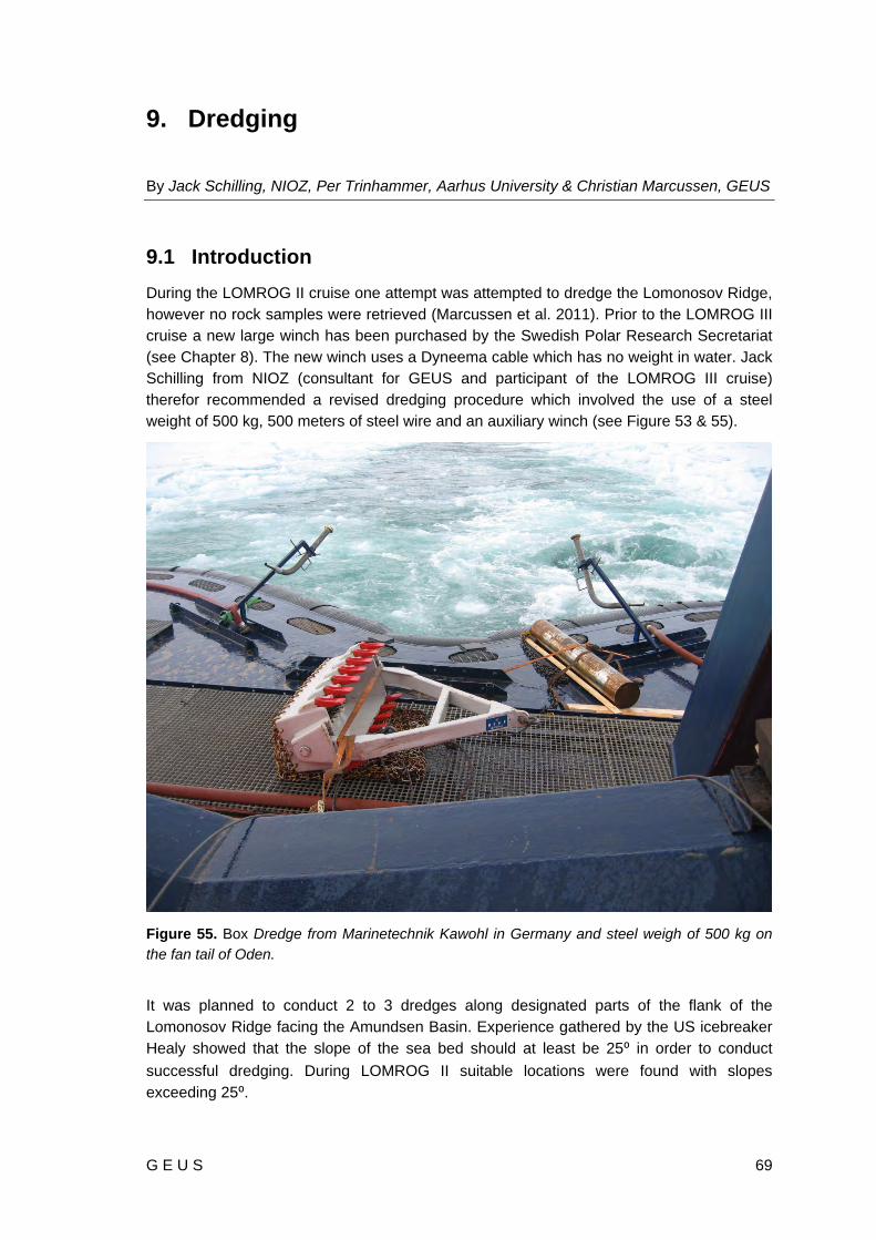
G E U S 69

9. Dredging

By Jack Schilling, NIOZ, Per Trinhammer, Aarhus University & Christian Marcussen, GEUS

9.1 Introduction During the LOMROG II cruise one attempt was attempted to dredge the Lomonosov Ridge, however no rock samples were retrieved (Marcussen et al. 2011). Prior to the LOMROG III cruise a new large winch has been purchased by the Swedish Polar Research Secretariat (see Chapter 8). The new winch uses a Dyneema cable which has no weight in water. Jack Schilling from NIOZ (consultant for GEUS and participant of the LOMROG III cruise) therefor recommended a revised dredging procedure which involved the use of a steel weight of 500 kg, 500 meters of steel wire and an auxiliary winch (see Figure 53 & 55).

Figure 55. Box Dredge from Marinetechnik Kawohl in Germany and steel weigh of 500 kg on the fan tail of Oden.

It was planned to conduct 2 to 3 dredges along designated parts of the flank of the Lomonosov Ridge facing the Amundsen Basin. Experience gathered by the US icebreaker Healy showed that the slope of the sea bed should at least be 25⁰ in order to conduct successful dredging. During LOMROG II suitable locations were found with slopes exceeding 25⁰.

70 G E U S

9.2 Procedure Before the dredging commenced the dredging procedure was discussed in detail with the ship’s crew. It was decided to use the ice drift for our attempts to dredge which had the obvious advantage that Oden had not to break a lead beforehand. A detailed description of the procedure used during dredging is included in Appendix V (Section 19.5). The most important issue of the procedure is to pay out cable with the same speed as the ships is doing and not faster to avoid too much cable on the seabed.

9.3 Results

9.3.1 Dredge 1

Dredge 1 started on 19 August 2012 at 16:51 (UTC) and lasted for approx. 5½ hours. A log is included in Appendix V (Section 19.5). The dredge covered a depth range from approx. 3400 m to 2020 m (Figure 56). Operations went very smoothly and approx. 100 kg of rock samples were gathered. Based on a first visual inspection the rock samples are believed to be from an outcrop. Nearly all samples are covered by some kind of ferromanganese (?) crust (Figure 57). One or two dropstones were found. All samples were cleaned superficially and packed in 12 bags for shipment.

Figure 56. Bathymetric map based on multi beam data with Oden’s track during dredge 1. The direction of the ice drift up-dip on the flank of the Lomonosov Ridge was favourable for dredging. For location of the dredge see Figure 1.

G E U S 71

Figure 57. Retrieval of dredge 1 and some examples of the rock samples gathered.

9.3.2 Dredge 2

Figure 58. Bathymetric map based on multi beam data with Oden’s track during dredge 2. The direction of the ice drift up-dip on the flank of the Lomonosov Ridge was not as favourable for dredging as for dredge 1; nevertheless the dredge was successful. For location of the dredge see Figure 1.

72 G E U S

Dredge 2 started 20 August 2012 at 11:26 (UTC) and lasted for approx. 4½ hours. A log is included in Appendix V (Section 19.5). The dredge covered a depth range from approx. 3500 m to 2000 m (?) (Figure 58). Operations went very smoothly and approx. 200kg of rock samples were gathered. Mud in the dredge was flushed out. Based on a first visual inspection the rock samples are believed to be from an outcrop. Nearly all samples are covered by some kind of ferromanganese (?) crust (Figure 59). One large stone (“LOMROCK”, approx. 80 kg) was encountered. All samples were cleaned superficially and packed in 10 bags for shipment. The large rock was handled separately.

Figure 59. Retrieval of dredge 2 and some examples of the rock samples gathered. The photo in the lower right shows a large rock (“LOMROCK”) sampled during dredge 2.

9.4 References Marcussen, C. & LOMROG II Scientific Party 2011: Lomonosov Ridge off Greenland

(LOMROG II) – Cruise Report. Danmarks og Grønlands Geologiske Undersøgelse Rapport 2011/106, 154 pp.

G E U S 73

10. Oceanography

By Steffen M. Olsen & Rasmus Tonboe, Danish Meteorological Institute (DMI)

10.1 Introduction The oceanographic program carried out during the LOMROG III 2012 cruise includes collection of water column profiles with CTD (Conductivity, Temperature and Depth) and water sampling. Measurements have served a twofold purpose:

to support the seismic and hydrographic activities of the Continental Shelf Project of the Kingdom of Denmark

to assist and support the Swedish research projects organized by the Swedish Polar Research Secretariat and when possible, the Danish science of opportunity projects.

Knowledge of water mass distribution affecting the water column sound-velocity profile is required for proper interpretation and correction of the seismic data. The sonar mapping of the seafloor bathymetry also builds on this oceanographic information from the water column. The primary purpose of the oceanographic work is to supply representative, near real time water column profiles of sound velocity derived from CTD measurements.

Data are collected mainly from ice-stations (Figure 60) making use of Oden’s helicopter and modular, portable equipment. Ship stations (Figure 61) have also been conducted on an opportunistic basis. Water sampling at a number of ocean depth levels has also been part of the program, both for ship and ice station. Expendable CTD probes capable of measuring while steaming have been used twice during periods of transit. Their performance is not accessed.

The area of interest of the LOMROG III expedition spans the gradual transition towards more freshwater entrained upper water-masses crossing from the Amundsen Basin to the transition zone along the Lomonosov Ridge. At the same time, the deeper structure varies with the ageing of warmer water below and with different admixtures of basin specific deep waters. Frontal structures are typically not sharp in these regions of the Arctic and eddy features are relatively rare. In summer, the upper stratification is very complex with highly stable interfaces which are challenging to measure and with characteristics and spatial extent known to vary strongly inter-annually. The position of most stations has been planned ad-hoc taking into account the advance of Oden and the target area of the day. The overall strategy has been to form sections of station spacing of 20-40 NM with larger spacing on the abyssal plain. Denser cross isobath spacing is needed near bathymetric features known to guide ocean dynamics. This strategy has to some extent been successful and the station net spans the area of study and transit routes (Figure 63).

Oceanographic data acquired during the cruise are expected to contribute to the understanding of the processes maintaining the climatically important upper ocean halocline structure of the Arctic Ocean and yield valuable insight to “the state of the Arctic”. Of particular interest to the science team from DMI is the contribution of individual water

74 G E U S

masses to the layering between the upper mixed layer below the sea ice and the layer of warm, saline Atlantic inflow below. For this purpose, additional sensors (Oxygen, Fluorescence) have been added to the CTD probe. In order to facilitate a detailed analysis, bottle samples at a predefined set of depths levels has been recovered and stored for post cruise analysis. Data describe the physical environment and will also be integrated in the work of a number of the Danish and Swedish bio-science projects participating in LOMROG III.

10.2 Equipment and Methods Ice stations reached by helicopter made use of a modular, portable system supplied by the Section for Polar Oceanography, Danish Meteorological Institute (Figure 60). The system consists of a self-contained SBE19plusV2 pumped CTD configured in profiling mode (4Hz) in combination with a portable winch with 2000 m non-conductive Dyneema© line, an electric motor, controls and generator. Auxiliary sensors include a SBE 43 Oxygen probe and a SeaPoint Fluorometer. The system is depth rated to 3500 m. Water bottle samples were collected using a single 2.7 l Niskin type water sampler by drop-messenger triggering. On ice, the system is assembled and placed with the boom reaching over a lead.

After deployment, the SBE19 rests at 7 m for up to 10 minutes before being raised to the surface and starting the descent to a maximum depth of 2020 m. At shallower stations, care is exercised not the get contact with the bottom. The descent rate for the full profile was adjusted to approximately 30 m/min. The setup allows to profile up to the ice-ocean interface and into the brackish waters of the leads. Profiles resolve the layering in the undisturbed water column starting 70 cm below surface, and in this respect the setup is superior to ship based station work. Water bottle samples were drawn from the Niskin for isotopic composition (δ18O) and nutrient (N) at seven predefined depths down to 200 m covering the Arctic mixed layer and halocline.

Measurements of water mass distribution were done at full depth from Oden making use of a SBE911plus CTD-rosette system (Figure 61). The instrumentation were partly owned by DMI and partly by the University of Gothenburg and made available for the Continental Shelf project. This ship based system consists of a SeaBird rosette water-sampler equipped with 24 l Niskin type bottles, a SBE9plus CTD (24Hz) and a SBE11plus Deck Unit. The dual sensor sets includes pumped Temperature-Conductivity packages (TC duct and 3000 rpm pump) and a Benthos 200kHz altimeter.

After deployment, the CTD rested in the surface layer (10 m) for approximately 5 minutes after the pump turned on and sensor readings equilibrated. Hereafter the CTD and water sampler were raised to 1-2 m where data acquisition was started. Profiles were retrieved with a descent rate of 30 m/min in the upper 400 m, roughly across the strong upper ocean stratification and through the Atlantic Layer characterized in regions by sharp interleaving features. Below strong gradients in water mass properties, the descent rate was increased to 50 m/min in consideration of the limited station time available. Water samples were taken at predefined depths during the up-cast waiting 2 minutes at each depth before closing of bottles. Up-cast winch speed was 70 m/min. On deck, samples were drawn from the bottles for salinity, isotopic composition (δ18O) and nutrients.

G E U S 75

Station work was only attempted within the sea ice and made use of the a-frame and winch system on the fore deck. Engines were stopped and Oden typically drifted with a speed of 0.1-0.3 knots over ground with the ice drift. Thrusters were used to keep the area in front of Oden free from ice. All systems worked well during all stations but the line feed on the winch is still not fixed (Figure 62), a problem also realized during LOMROG II 2009 and EAGER 2011. Noise from the winch indicates that the ball bearings are damaged too.

Figure 60. Ice station, CTD and plankton sampling. From left, Pilot and bear watch Sven Stenwall, Rasmus Tonboe and Kajsa Tönnesen.

76 G E U S

Figure 61. Ship station with CTD and water sampling using a 24 bottle rosette. Winch and frame operated by Rasmus Tonboe.

Figure 62. Close up of the CTD winch above the main lab showing evolving problems towards the end of the cruise with the adjustment of the wire guide.

G E U S 77

10.3 Results

Date Time UTC Longitude Latitude Cast Type Sensors Station ID dd-mm-yyyy hh:mm ddd:mm.mm dd:mm.mm m LR12s01 02-08-2012 11:35 014:55.98 E 82:57.48 N 2625 Ship T/S LR12h01 03-08-2012 15:30 013:20.25 E 84:32.14 N 1889 Heli T/S/O/Chl LR12h02 04-08-2012 12:21 006:27.48 E 85:33.07 N 2012 Heli T/S/O/Chl LR12s02 05-08-2012 17:03 001:57.31 E 86:44.59 N 4248 Ship T/S LR12h03 06-08-2012 14:40 003:27.35 W 87:02.38 N 1996 Heli T/S/O/Chl LR12h04 07-08-2012 23:20 013:27.91 W 87:19.50 N 2006 Heli T/S/O/Chl LR12h05 08-08-2012 21:23 026:58.48 W 87:44.27 N 1996 Heli T/S/O/Chl LR12s03 09-08-2012 13:09 037:45.45 W 87:46.20 N 3746 Ship T/S LR12h06 10-08-2012 12:19 047:44.52 W 87:45.14 N 2014 Heli T/S/O/Chl LR12h07 11-08-2012 12:01 058:53.27 W 87:39.47 N 1209 Heli T/S/O/Chl LR12h08 12-08-2012 15:00 068:55.88 W 87:38.35 N 1128 Heli T/S/O/Chl LR12h09 13-08-2012 19:27 043:10.52 W 88:15.93 N 2010 Heli T/S/O/Chl LR12h10 14-08-2012 17:30 029:57.05 W 88:14.09 N 2018 Heli T/S/O/Chl LR12h11 15-08-2012 14:20 058:01.00 W 88:16.32 N 1507 Heli T/S/O/Chl LR12s04 16-08-2012 05:10 069:24.69 W 88:20.80 N 1197 Ship T/S LR12h12 17-08-2012 17:49 057:33.00 W 88:38.10 N 1993 Heli T/S/O/Chl LR12h13 18-08-2012 12:30 079:18.13 W 89:00.80 N 1084 Heli T/S/O/Chl LR12s05 20-08-2012 05:10 058:50.83 W 89:15.90 N 3731 Ship T/S LR12h14 20-08-2012 14:08 068:01.76 W 89:08.16 N 1924 Heli T/S/O/Chl LR12h15 21-08-2012 18:24 090:53.25 W 88:53.78 N 1223 Heli T/S/O/Chl LR12h16 22-08-2012 17:21 155:31.52 E 89:59.55 N 2003 Heli T/S/O/Chl LR12h17 23-08-2012 13:22 133:12.10 E 89:30.44 N 2006 Heli T/S/O/Chl LR12x01 24-08-2012 10:37 136:54.11 E 88:42.43 N 1166 XCTD T/S LR12h18 24-08-2012 15:15 149:59.50 E 88:24.73 N 1850 Heli T/S/O/Chl LR12h19 24-08-2012 22:07 145:16.56 E 88:03.58 N 1243 Heli T/S/O/Chl LR12x02 25-08-2012 03:31 135:19.47 E 87:57.31 N 495 XCTD T/S LR12h20 25-08-2012 08:09 124:55.48 E 87:56.07 N 1992 Heli T/S/O/Chl LR12h21 25-08-2012 18:12 114:41.68 E 87:52.88 N 1981 Heli T/S/O/Chl LR12h22 26-08-2012 17:53 104:30.29 E 87:59.35 N 1994 Heli T/S/O/Chl LR12s06 27-08-2012 11:21 078:14.56 E 88:08.96 N 4354 Ship T/S LR12h23 29-08-2012 15:29 070:10.86 E 88:17.53 N 1991 Heli T/S/O/Chl LR12h24 30-08-2012 15:52 056:02.99 E 88:45.11 N 2009 Heli T/S/O/Chl LR12s07 31-08-2012 13:56 053:06.18 E 88:47.43 N 4351 Ship T/S LR12h25 02-09-2012 08:30 025:17.19 E 88:16.87 N 2022 Heli T/S/O/Chl LR12h26 03-09-2012 13:20 011:21.11 E 88:09.54 N 2003 Heli T/S/O/Chl LR12h27 04-09-2012 10:25 027:16.14 E 87:49.71 N 2004 Heli T/S/O/Chl LR12h28 05-09-2012 08:26 018:58.52 E 87:28.24 N 1991 Heli T/S/O/Chl LR12s08 07-09-2012 06:44 005:16.63 E 85:25.59 N 3093 Ship T/S LR12s09 08-09-2012 07:36 003:43.29 E 84:22.21 N 3779 Ship T/S LR12s10 09-09-2012 06:46 015:10.37 E 83:49.41 N 4000 Ship T/S LR12h29 09-09-2012 15:00 014:59.31 E 83:28.32 N 1999 Heli T/S/O/Chl LR12s11 10-09-2012 06:23 014:44.67 E 82:46.12 N 1457 Ship T/S LR12s12 11-09-2012 06:16 008:45.12 E 82:11.75 N 719 Ship T/S LR12s13 11-09-2012 16:01 008:35.89 E 81:51.81 N 747 Ship T/S

Table 6. CTD stations acquired during LOMROG III

78 G E U S

In total 29 ice stations (Table 6 & Figure 63) were all completed successfully using 4 hours on the ice at each station. Despite the latitudes of operation, conditions were not harsh compared with areas and seasons where the system has also been operated with success. Ice drift of up to 0.6 knots has been experienced and required careful selection of the station location. Helicopter pilots from Kalax Flyg (SE) very skilfully identified suitable floes for landing.

13 ship stations were completed during the cruise (Table 6 & Figure 63). A number of science projects sampled the rosette and were involved in the water budget planning at each station.

10.4 Data Processing and Work Flow Using SeaBird SeaSoft software, raw data from the CTD (HEX format) are converted into engineering units including pressure, in situ temperature and conductivity. Pressure readings are initially high pass filtered two ways in order to smooth high frequency data and to obtain a uniform descent history of the cast. The applied cut-off period for the SBE9plus and SBE19plusV2 are 0.15 sec and 1 sec, respectively. For the SBE19plusV2, also temperature and conductivity are filtered with a cutoff of 0.5 sec. Inherent misalignment due to time delay in sensor responses and transit time delay in the pumped pluming line are corrected by advancing conductivity 0.073 sec relative to pressure for the SBE9plus (programmed in the SBE11 unit) and +0.5 sec for the SBE19plusV2 unit. By this alignment, measurements refer to same parcel of water and the procedure eliminates artificial spikes in the calculated salinity which is dependent on temperature, pressure and conductivity. A recursive filter was hereafter applied to remove cell thermal mass effects from the measured conductivity according to the specifications for the individual sensors of the CTD systems. This correction of salinity is significant in the upper layers with steep temperature gradients, but otherwise negligible. The last modification of the data removes scans with slow descent rate or reversals in pressure.

Processed data are averaged into 1 m bins and derived parameters include salinity and sound velocity. Data files are immediately uploaded to a shared archive and hydrographers notified and advised on the bridge. Daily graphics files were prepared with emphasis on the evolution of the sound velocity along Oden’s track. An example is given in Figure 22.

10.5 Quality Control and Data Accuracy From ship CTD station samples were taken for on-board bottle salinity reference measurements. With replicates, 40 individual samples have been measured onboard yielding satisfactory statistics for performing post cruise corrections of the raw data files if needed. Bottle salinities were measured using an Autosal Guildline 8410 portable lab salinometer with a nominal precision of 0.003 PSU. IAPSO standard seawater references were used purchased prior to the cruise from OSIL (www.oscil.co.uk): Batch: P153, K15=0.99979, Practical Salinity 34.992 and to be used by 8 March 2014. The salinometer was placed in stable temperature environment of 21ºC and left to warm up 24 hours prior to reference setting, zero calibration and standardization procedures immediately preceding

G E U S 79

the analysis. Bath temperature (23ºC) was set to two degrees above ambient temperature. The bottle samples were analysed in one series near the end of the cruise. Negligible drift (0.002 PSU or less) could be identified during the sequence of analysis. Three readings were performed for each bottle and the mean error between CTD salinity and bottle salinities could be estimated with at precision of 0.004. The slope correction determined for the SBE911 system based on the bottle data statistics yields corrections smaller than the nominal error of the salinometer and conductivity sensor (+/-0.002). On this basis, it has not been considered to correct the calibration coefficients for conductivity. Nominal temperature sensor accuracy is +/- 0.001ºC with an instrument resolution of about 0.0003ºC. The real accuracy is likely better than the nominal temperature accuracy judging from the weak drift of the sensor between calibrations. We obtained acceptable near zero pressure readings on deck and consider the relevant uncertainty for the dataset to increase to from zero to approximately 1.2 m at 4000 m depth.

Correspondence between SBE9plus and SBE19plus sensors can only be evaluated by comparing neighbouring stations (e.g. S07 and H27). Differences below 1000 m are less than 0.004 PSU and 0.02K which is also within expected real ocean variability. This may be taken as an upper estimate of the data uncertainty for the compiled dataset. It is emphasized that all sensors have recently been calibrated at SeaBird facilities. This estimate does not include XCTD measurements.

10.6 Data Ownership and Access The dataset is owned by the Continental Shelf Project and held by the Danish Meteorological Institute with the right to use and publish the dataset in scientific literature. Data may not be published or distributed without permission from DMI (contact [email protected]).

80 G E U S

Figure 63. CTD station map showing ship (S), expendable probes (X) and helicopter (H) ice stations recovered during LOMROG III.

G E U S 81

11. Plankton Ecology

By Kajsa Tönnesson, University of Gothenburg & Tanja Statmann, Aarhus University

11.1 Introduction The effect of environmental changes on the biological pelagic system in the central Arctic Ocean is difficult to estimate due to limited available data. The central Arctic Ocean is characterized by the most extreme seasonal light regime of all marine systems (Auel & Hagen 2002). The primary production, which is mainly composed of ice algae and pelagic phytoplankton, forms the base of the food web thus supporting organisms at higher trophic levels. The amount and distribution of phytoplankton is therefore likely to affect the behaviour and distribution of zooplankton. Herbivorous zooplanktons are the primary grazers on the phytoplankton biomass. Previous investigations of the central Arctic Ocean have found two Calanus (C. glacialis and C. hyperboreus (Figure 62)) and one Metridia species (M. longa) to account for a substantial part of the zooplankton biomass (Mumm 1993; Kosobokova and Hirche 2000; Auel and Hagen 2002). In particular Calanus species, with high energy content in the form of lipids (Swalethorp et al. 2009), are important prey items for larger carnivorous zooplankton, fish larvae, fish, birds and whales (Falk-Petersen et al. 2007; Laidre et al. 2007).

Carnivorous zooplankton might have a substantial impact on prey communities. The large carnivorous copepod Pareuchaeta is common in the central Arctic Ocean (Mumm 1993; Kosobokova & Hirche 2000; Auel & Hagen 2002) and could play an important role in the predation on small copepods.

Zooplankton, both herbivores and carnivores, modify the prey community by grazing and predation. Zooplankton will also have an impact on the benthic-pelagic coupling through sedimentation of organic aggregates. The trophic structure of the heterotrophic community is important in determine what fraction of the primary production is exported from the surface to the deep ocean and the sediment. One of the main mechanisms is the vertical flux of zooplankton fecal pellets. Due to their high sinking speeds, large particles are not consumed or remineralised in the water column as readily as small, suspended particles. Therefore, these organisms may represent an important mechanism coupling the pelagic system with the benthic community. Apart from fuelling the benthos part of the organic material is buried thus this fecal pellet flux also acts as a carbon sink from the atmosphere to the deep sea sediments.

The primary focus of most previous studies has been to describe the mesozooplankton species composition, abundance and vertical distribution in relation to different water masses and basins or with a temporal resolution to describe seasonal changes. Investigations including phytoplankton, protozooplankton, mesozooplankton and the predatory interaction between or within them are however scarce. The relatively importance of the different components of the Arctic zooplankton community for grazing, predation and sedimentation is not very well investigated. Data on how these trophic interactions

82 G E U S

responds to environmental change are also required for better understanding the dynamics of Arctic pelagic ecosystems.

Figure 64. Calanus hyperboreus. Photo: Pauline Snoeijs Leijonmalm.

During the cruise sampling of plankton was carried out in the Nansen, Amundsen and Makarov basins, on transects across the Gakkel and Lomonosov Ridges. By sampling and experiments we will:

Describe the structure, distribution and biomass of phytoplankton, proto-zooplankton and meso-zooplankton in the surface water (0-250 m).

Determine the grazing pressure of the most dominating copepods, Calanus finmarchicus, C. hyperboreus and Metridia sp. as well as the whole community.

Determine the diet and the predation impact of invertebrate predators (chaetognaths and predatory copepods).

Quantify zooplankton’s contribution to the vertical flux.

Measure the astaxanthin and thiamine levels in dominant Arctic copepods (C. glacialis, C. hyperboreus, M. longa). Study conducted together with Pauline Snoeijs Leijonmalm and Peter Sylvander.

Examine specific predator prey relationships, through stable isotopes used as trophic markers in C. glacialis, C. hyperboreus, M. longa and Pareuchaeta sp. as well as in their possible food sources (Phytoplankton and Protozooplankton). Study conducted together with Pauline Snoeijs Leijonmalm and Peter Sylvander.

Study whether environmental stress such as unfavourable levels of light, temperature and salinity increase the demand of thiamine and astaxanthin

G E U S 83

compounds in the copepod C. hyperboreus. Experiments together with Pauline Snoiejs Leijonmalm and Peter Sylvander.

Investigate the distribution and characteristics of dissolved organic matter (DOM) in the Arctic Ocean and in particular if degradation of DOM in the deep oceans are controlled by the conditions in the deep oceans or governed by the low quality of the DOM at great depth.

11.2 Methods

11.2.1 Net Sampling

The vertical distribution of mesozooplankton was investigated by multiple opening-closing net hauls from Oden and ice borne stations reached by helicopter. In total 42 stations along the cruise track were sampled in the Nansen and the Amundsen basins and across the Gakkel and Lomonosov Ridges (13 times from the ship and 29 times from ice borne stations, Table 7a & Figure 63). Stratified samples were collected in 0-50, 50-100, 100-150,

Figure 65. The MultiNet used for sampling of Meso-zooplankton in five different depth intervals (Photo: Ragnar Jerre).

84 G E U S

150-200 and 200-250 m depths intervals from the ship (MultiNet, mesh size 45 µm, Figure 63) and 0-50 and 0-100 m from the ice borne stations (WP-2 net¸ mesh size 45 µm and 450 µm, Figure 66 and 67). All samples were preserved in a 4% formaldehyde/seawater solution and will be analysed with regard to abundance, biomass and species composition after the cruise.

Figure 66. Ice station. Rasmus Tonsboe and Steffen M. Olsen checking the integrity of the ice.

11.2.2 Water Sampling

From the ship, water was collected from eight depths (10, 20, 40, 60, 100, 150, 200 and 300 m) using a 24-bottle rosette sampler equipped with 7.5 l Niskin bottles (13 stations, Table 7b). Seven of these depths (10, 20, 40, 60, 100, 150 and 200 m) have also been sampled from ice borne stations with a 2.7 l Niskin bottle (Figure 66, Table 7b). Water was drawn for total nitrogen and phosphorous, inorganic nutrients, protozooplankton (dinoflagellates and ciliates) and chlorophyll a. In addition, at 9 stations (Table 8) suspended fecal pellets were collected at 3 depths (10, 20 and 40 m). The samples for inorganic nutrients (phosphate, nitrate, nitrite, ammonia, and silicate) were collected directly from the water sampler and immediately frozen (-18⁰C) for post cruise analyses. Samples for protozooplankton were taken at 5 depths (10, 20, 60, 100 and 200 m) at all 42 stations and preserved with 2% acidified Lugol’s solution for analyses after the cruise. Water samples were taken at 42 stations for chlorophyll a measurements. Water (500 – 1500 ml) was filtered onto filters (GF/F, 11 μm and 50 μm) which then were extracted in 5 ml 96% ethanol for 24 hours and kept frozen for post cruise fluorometrical analyses.

G E U S 85

Figure 67. Ice station. Zooplankton sampling 0-100 m with the WP-2 net. In the photo: Kajsa Tönnesson, Steffen M. Olsen and Rasmus Tonboe (Photo: Sven Stenvall).

Figure 68. Ice station. Steffen M. Olsen is preparing the Niskin bottle for water sampling.

86 G E U S

LOMROG III Date Longitude Latitude

Station ID yyyy‐mm‐dd ddd:mm.mm dd:mm.mm 0‐100m 0‐50m 50‐100m 100‐150m 150‐200m 200‐250m

LR12s01 02‐08‐2012 014:55.98 E 82:57.48 N M M M M M

LR12h01 03‐08‐2012 013:20.25 E 84:32.14 N WP WP

LR12h02 04‐08‐2012 006:27.48 E 85:33.07 N WP WP

LR12s02 05‐08‐2012 001:57.31 E 86:44.59 N WP

LR12h03 06‐08‐2012 003:27.35 W 87:02.38 N WP WP

LR12h04 07‐08‐2012 013:27.91 W 87:19.50 N WP WP

LR12h05 08‐08‐2012 026:58.48 W 87:44.27 N WP WP

LR12s03 09‐08‐2012 037:45.45 W 87:46.20 N M M M M M

LR12h06 10‐08‐2012 047:44.52 W 87:45.14 N WP WP

LR12h07 11‐08‐2012 058:53.27 W 87:39.47 N WP WP

LR12h08 12‐08‐2012 068:55.88 W 87:38.35 N WP WP

LR12h09 13‐08‐2012 043:10.52 W 88:15.93 N WP WP

LR12h10 14‐08‐2012 029:57.05 W 88:14.09 N WP WP

LR12h11 15‐08‐2012 058:01.00 W 88:16.32 N WP WP

LR12s04 16‐08‐2012 069:24.69 W 88:20.80 N M M M M M

LR12h12 17‐08‐2012 057:33.00 W 88:38.10 N WP WP

LR12h13 18‐08‐2012 079:18.13 W 89:00.80 N WP WP

LR12s05 20‐08‐2012 058:50.83 W 89:15.90 N M M M M M

LR12h14 20‐08‐2012 068:01.76 W 89:08.16 N WP WP

LR12h15 21‐08‐2012 090:53.25 W 88:53.78 N WP WP

LR12h16 22‐08‐2012 155:31.52 E 89:59.55 N WP WP

LR12h17 23‐08‐2012 133:12.10 E 89:30.44 N WP WP

LR12h18 24‐08‐2012 149:59.50 E 88:24.73 N WP WP

LR12h19 24‐08‐2012 145:16.56 E 88:03.58 N WP WP

LR12h20 25‐08‐2012 124:55.48 E 87:56.07 N WP WP

LR12h21 25‐08‐2012 114:41.68 E 87:52.88 N WP WP

LR12h22 26‐08‐2012 104:30.29 E 87:59.35 N WP WP

LR12s06 27‐08‐2012 078:14.56 E 88:08.96 N M M M M M

LR12h23 29‐08‐2012 070:10.86 E 88:17.53 N WP WP

LR12h24 30‐08‐2012 056:02.99 E 88:45.11 N WP WP

LR12s07 31‐08‐2012 053:06.18 E 88:47.43 N M M M M M

LR12h25 02‐09‐2012 025:17.19 E 88:16.87 N WP WP

LR12h26 03‐09‐2012 011:21.11 E 88:09.54 N WP WP

LR12h27 04‐09‐2012 027:16.14 E 87:49.71 N WP WP

LR12h28 05‐09‐2012 018:58.52 E 87:28.24 N WP WP

LR12s08 07‐09‐2012 005:16.63 E 85:25.59 N M M M M M

LR12s09 08‐09‐2012 003:43.29 E 84:22.21 N M M M M M

LR12s10 09‐09‐2012 015:10.37 E 83:49.41 N M M M M M

LR12h29 09‐09‐2012 014:59.31 E 83:28.32 N WP WP

LR12s11 10‐09‐2012 014:44.67 E 82:46.12 N M M M M M

LR12s12 11‐09‐2012 008:45.12 E 82:11.75 N M M M M M

LR12s13 11‐09‐2012 008:35.89 E 81:51.81 N M M M M M

Integrated sampling: Zooplankton biomass

Table 7a. Station list (Ship stations (LR12s) and Ice stations (LR12h)), Zooplankton samples from the water column: Sampling with WP-2 net (WP) and MultiNet (M) (see also Figure 61 for a map with all stations).

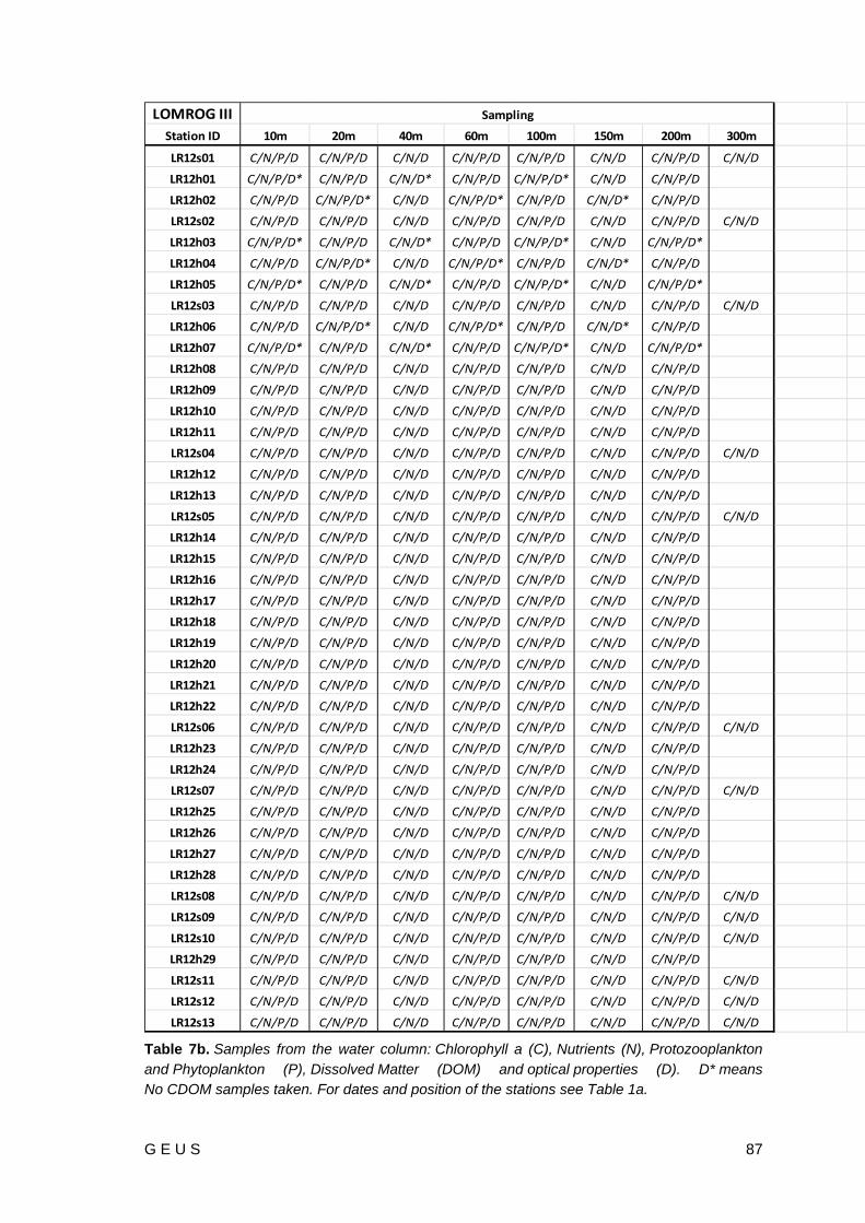
G E U S 87

LOMROG III

Station ID 10m 20m 40m 60m 100m 150m 200m 300m

LR12s01 C/N/P/D C/N/P/D C/N/D C/N/P/D C/N/P/D C/N/D C/N/P/D C/N/D

LR12h01 C/N/P/D* C/N/P/D C/N/D* C/N/P/D C/N/P/D* C/N/D C/N/P/D

LR12h02 C/N/P/D C/N/P/D* C/N/D C/N/P/D* C/N/P/D C/N/D* C/N/P/D


LR12h03 C/N/P/D* C/N/P/D C/N/D* C/N/P/D C/N/P/D* C/N/D C/N/P/D*






LR12h08 C/N/P/D C/N/P/D C/N/D C/N/P/D C/N/P/D C/N/D C/N/P/D
































Sampling

Table 7b. Samples from the water column: Chlorophyll a (C), Nutrients (N), Protozooplankton and Phytoplankton (P), Dissolved Matter (DOM) and optical properties (D). D* means No CDOM samples taken. For dates and position of the stations see Table 1a.

88 G E U S

11.2.3 Incubations

To understand how organic material and nutrients are channelled through the food web, it is important to quantify the rates (production, grazing, predation and sedimentation). Quantitative information on feeding rates is particularly important since they represent the major transfers of biomass within ecosystems. The methods to quantify grazing (predation) of zooplankton are numerous and during the LOMROG III cruise several methods (gut fluorescence, gut content analyses and pellet production) have been used. Most methods have strengths and weaknesses. The choice of which method to use is depending on the type of zooplankton and the ingested food (herbivory, omnivory and carnivory). The combination of several methods will give us important information on different aspects of food and feeding. Though some methods are more laborious than others (e.g. analyses of stomach contents) they are important since they can give information about food selection and prey-size preferences (or limitations).

Animals for experiments (Table 8 and 9) were obtained from the upper 60 m using a WP-2 net with a 450 µm mesh size. The content of the cod-end was then transferred to a thermo box and brought to the main laboratory on the fore-deck. Following experiments were conducted: Fecal pellet production, In situ pellet production (fecatron) and experiments to test the effect of environmental stress. Water used in incubations was collected with a Niskin bottle from the ice (10 m) or tapped from the seawater system (pumped from 10 m depth) located in the main laboratory on board Oden. Animals for chemical analyses (carbon, nitrogen, isotopes) were collected from the same net hauls.

11.2.4 Pellet Production Experiments

Pellets (egested material) are the part of the food that has not been absorbed by the digestive system of the animal. For copepods, which have pellets covered by a membrane, collection of fecal pellets is possible. Moreover, the number of pellets must show a clear relationship with feeding intensity and be independent of the type of food. To quantify ingestion, information about the pellet production rate and the relation between egested pellets and ingested food or absorption efficiency is needed.

11.2.4.1 Pellet Production and Feeding Rates for Three Dominating Copepods We conducted fecal production experiments with three dominating copepods (Calanus hyperboreus, C. glacialis and Metridia longa) on several stations during the cruise (38 stations with C. hyperboreus and C. glacialis, and 8 stations with M. longa). C. hyperboreus and C. glacialis females were individually transferred to 620 ml polycarbonate bottles containing 64 µm filtered seawater. M. longa females were transferred to 1500 ml fecatrons (with false 200 µm mesh bottom). The bottles/fecatrons were then incubated for 24 hours at in situ temperature (approximately -1 to -1.7ºC). After incubation the females length was measured and produced fecal pellets were counted and measured (Figure 69).

G E U S 89

Figure 69. Tanja Stratmann is taking down one of the 38 fecal pellets experiment.

11.2.4.2 In Situ Fecal Pellet Production The fecal pellet production of the copepod community was measured through short time incubations conducted at 8 stations (Table 8). On deck subsamples of the cod-end was immediately distributed into 4 fecatrons (PVC tubes with 400 µm false mesh bottom) filled with filtered sea water (Figure 68). The copepods were incubated 1-2 hours where after copepods and produced fecal pellets were preserved in acidic Lugol’s solution. At 9 stations, water samples for quantification of suspended fecal pellets were collected at 3 depths (10, 20 and 40 m). The water samples were concentrated on a 20 μm sieve, fixed in 2 % acidic Lugol’s solution for post cruise analyses.

11.2.4.3 Feeding Rates for Pareuchaeta sp. Feeding rates for Pareuchaeta sp. were measured indirectly by estimating pellet production since experimental studies have shown a linear relationship between food intake and number of pellets defecated. Within 1 hour of collection, individual Pareuchaeta sp. females or copepodites were transferred by pipette into 620 ml polycarbonate bottles filled with 64 μm filtered seawater. The bottles were incubated at 72 hours at in situ temperature (-1 to -1.7ºC). At the end of the incubations, the content was gently poured through a 45 μm sieve to collect animals and fecal pellets. The length of females or copepodites and the dimensions of the pellets were measured using a dissection microscope. Complementary studies to show possible selectivity will be performed through gut content analyses after the cruise. The experiments were conducted at 36 stations.

90 G E U S

G E U S 91

Tabl

e 8.

Lis

t of e

xper

imen

ts a

nd in

situ

mea

sure

men

ts c

ondu

cted

at d

iffer

ent s

tatio

ns. S

tatio

ns s

orte

d by

dat

e. F

P s

tand

s fo

r fe

cal p

elle

t pro

duct

ion.

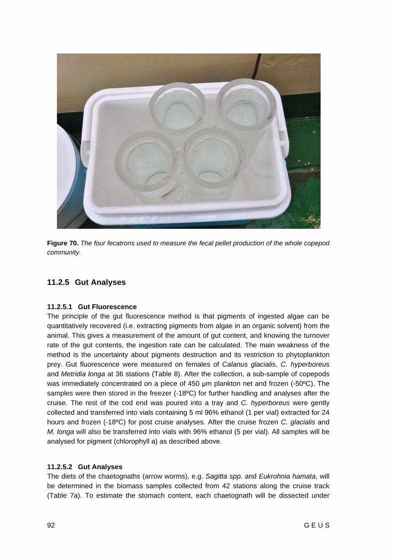
92 G E U S

Figure 70. The four fecatrons used to measure the fecal pellet production of the whole copepod community.

11.2.5 Gut Analyses

11.2.5.1 Gut Fluorescence The principle of the gut fluorescence method is that pigments of ingested algae can be quantitatively recovered (i.e. extracting pigments from algae in an organic solvent) from the animal. This gives a measurement of the amount of gut content, and knowing the turnover rate of the gut contents, the ingestion rate can be calculated. The main weakness of the method is the uncertainty about pigments destruction and its restriction to phytoplankton prey. Gut fluorescence were measured on females of Calanus glacialis, C. hyperboreus and Metridia longa at 36 stations (Table 8). After the collection, a sub-sample of copepods was immediately concentrated on a piece of 450 μm plankton net and frozen (-50ºC). The samples were then stored in the freezer (-18ºC) for further handling and analyses after the cruise. The rest of the cod end was poured into a tray and C. hyperboreus were gently collected and transferred into vials containing 5 ml 96% ethanol (1 per vial) extracted for 24 hours and frozen (-18ºC) for post cruise analyses. After the cruise frozen C. glacialis and M. longa will also be transferred into vials with 96% ethanol (5 per vial). All samples will be analysed for pigment (chlorophyll a) as described above.

11.2.5.2 Gut Analyses The diets of the chaetognaths (arrow worms), e.g. Sagitta spp. and Eukrohnia hamata, will be determined in the biomass samples collected from 42 stations along the cruise track (Table 7a). To estimate the stomach content, each chaetognath will be dissected under

G E U S 93

microscope, and prey organism will be identified to species level and stage. Analyses of stomach contents of field sampled zooplankton are a common method for estimating ingestion rate of carnivorous zooplankton. Prey composition and production will be used to estimate predation pressure and selectivity.

11.2.6 Sediment Traps

Vertical carbon flux depends as heavily on hydrography, variations of nutrients and primary production (bottom-up) as on the dynamics of the zooplankton (top-down). One of the main mechanisms is the vertical flux of zooplankton faecal pellets. Zooplankton can consume a large fraction of the daily primary production and as a consequence contribute significantly to the downward carbon flux, through the production of carbon-rich fecal pellets with high sinking rates. Due to their high sinking speeds, large particles are not consumed or remineralised in the water column as readily as small, suspended particles.

We determined the fecal pellets carbon content and sinking rates, and combine this information with measured feeding rates and abundances to estimate pellet fluxes to different zones in the water column. The vertical flux of pellets were measured by using in situ free floating sediment traps 6 times from ice borne stations and from the ship (Table 8). The traps were deployed at three different depths (10, 20 and 40 m), with a deployment time of 4 hours (Figure 71). Prior to deployment, the traps were filled with 0.2 μm filtered seawater with added salt to increase the salinity by 4-5 psu. Hereby, advective diffusive exchange between the higher density, particle-free water and the ambient seawater was reduced in the traps during deployment. No preservative was added. Immediately after recovery, the sedimentation traps were sealed with a clean lid and the trap content carefully mixed. In the laboratory, subsamples for chlorophyll a and fecal pellets analyses were taken.

94 G E U S

Figure 71. Ice station. Recovery of the sediment traps (Photo: Steffen M. Olsen).

11.2.7 Dissolved Organic Matter

The aim of the project is to investigate the distribution and characteristics of dissolved organic matter (DOM) in the Arctic Ocean and in particular if degradation of DOM in the deep oceans are controlled by the conditions in the deep oceans or governed by the low quality of the DOM at great depth.

11.2.8 The Role of Environmental Conditions for Degradation of DOM

The objective for this experiment is to test if degradation of DOM in the deep ocean is governed by characteristics of the DOM-pool or by environmental conditions. This will be tested in the laboratory after the cruise by manipulating temperature and other conditions. During the cruise large volumes of water were collected from the deeper part if the Arctic Ocean at 5 stations (Table 8) for degradations experiments during the winter 2012/2013. Samples for bacteria community analyses have also been taken at 5 stations.

11.2.9 Distribution and Characteristics of DOM in the Arctic Ocean

The objective is to describe the distribution of the following parameters:

Concentrations of DOC, DON and DOP

DOM absorption – 300 to 700 nm

G E U S 95

DOM fluorescence from excitation – emission scans

Samples were taken from all stations and depths (Figure 70, Table 7b). We followed the sampling scheme already decided on LOMROG II (10, 20, 40, 60, 100, 150, 200 and 300 m) with addition of deeper samples (500, 1000, 1500, 2000, 2500 m ...). All depths are not shown in Table 7b. Samples will be analysed for dissolved organic carbon (DOC) and optical properties (scanning absorption and excitation-emission fluorescence). Data will be analysed for relationships to physical, chemical and biological parameters and can acts as supporting data for other experiments/projects.

Figure 72. Tanja Stratmann is taking samples for DOM and absorption in the clean laboratory.

96 G E U S

11.3 Projects Together with Pauline Snoeijs Leijonmalm and Peter Sylvander, Stockholm University

11.3.1 A Comparison of Astaxanthin and Thiamine Levels in Dominant Arctic and Baltic Zooplankton Species

Our hypothesis is that the dominant phytoplankton and zooplankton species in the Arctic Ocean have higher levels of astaxanthin (antioxidant) and thiamine (vitamin and antioxidant) than those of the Baltic Sea. Copepods were obtained from the upper 60 m using a WP-2 net with a 450 µm mesh size (Table 8). Direct after sampling, 20 females of the dominant species (Calanus hyperboreus, C. finmarchicus and Metridia longa) were measured and frozen (-80ºC) for post cruise analyses. Filters for phytoplankton were taken simultaneously. Samples were taken at 14 stations.

11.3.2 Trophic Levels of Dominant Arctic Zooplankton Species in Summer: Evidence from Stable Isotopes Signature

The trophic position of an organism within a food web and its basic carbon source may be derived from nitrogen and carbon stable isotope ratios. Our hypothesis is that the dominant zooplankton species in the arctic belong to different trophic levels (trophic level ranking of dominant species). Even if different factors affect this (e.g. season, levels of food), the δ13C, δ15N markers indicates the trophic level very well with different species in the same area and the same season are compared.

At 35 stations (Table 8), females of Calanus hyperboreus, C. glacialis, Metridia longa and Pareuchaeta sp. (not all species at all stations) were gently collected and transferred into bottles with filtrated water for 24 hours. The females were then washed in Milli-Q water and frozen at -80ºC, each in a separate eppendorf tube for post cruise analyses. A number of phytoplankton filters were taken simultaneously.

11.3.3 The Effect of Environmental Stress on Antioxidant Depletion in Calanus hyperboreus

Thiamine (vitamin B1) and astaxanthin are both compounds which act as antioxidants and are involved in basic stress response in plants and animals. Animals are not capable of de novo synthesis of these compounds and therefore depend on nutritional sources of either the complete compound (thiamine) or precursors (astaxanthin) to maintain body concentrations. In several aquatic systems, animals have shown signs of deficiency of these compounds of reasons not yet fully elucidated. In this project we studied whether environmental stress such as unfavorable levels of light, temperature and salinity increase the demand of these two compounds in the copepod Calanus hyperboreus. Since de novo synthesis is not possible without a food source we incubated the herbivore C. hyperboreus in filtered seawater devoid of phytoplankton. Decreased body concentrations can therefore be considered to be a result of increased depletion rather than decreased synthesis/uptake.

G E U S 97

We hypothesize that C. hyperboreus subjected to environmental stress will deplete thiamine and astaxanthin at a higher rate than individuals subjected to more favorable conditions.

Calanus hyperboreus was collected from the ship or ice borne stations with a WP-2 net with a 450 µm mesh size from a depth of 60 m (Table 8). 24 adult females were measured and transferred to -80ºC to later be used as control samples (Figure 73). 72 adult females were then measured and transferred to 500 ml bottles containing GF/F filtered seawater, one individual per bottle. 36 of the collected individuals were incubated in darkness at 3ºC by covering the bottles in black plastic and putting them in refrigerators. The remaining 36 individuals were subjected to a stress treatment. In total, 6 experiments were carried out with three different kinds of stress factors. As stress treatment, high light, high temperature or decreased salinity was used (Table 9). Light stress was acquired by excluding the black plastic cover over the bottles. Temperature stress was acquired by incubating bottles in at room temperature. Salinity stress was acquired by diluting filtered sea water with fresh water. 12 individuals of both the stressed and the non-stressed females were collected 12, 24 and 24 hours after the experiment was set up, by pouring the bottle content through a small hand held sieve. At the same time, the water of the bottles was filtered over a GF/F filter and fecal pellets were counted. Both the female and the GF/F filters were transferred to -80ºC. Astaxanthin and thiamine content of both the collected females and filters will be analysed by means of high performance liquid chromatography (HPLC) at the Department of Systems Ecology, Stockholm University. Analysis of the animals will show the thiamine- and astaxanthin content of the body tissues at sampling time while the analysis of the GF/F filters will show if any significant amounts have been excreted in e.g. fecal pellets or eggs.

Figure 73. Experimental work in the main laboratory. Peter Sylvander and Pauline Snoeijs Leijonmalm are setting up one of the experiments.

98 G E U S

Experiment Sampling position

Used stress factor

Light (µmol m-2 s-1)

Temperature (ºC)

Salinity (psu)

1 87º46.20 N 37º45.45 W

Light 0/150 3 35

2 89º15.90 N 58º50.83 W

Light 0/150 3 35

3 88º47.43 N 53º06.18 E

Temperature 0 3/16 35

4 87º28.24 N 18º58.52 E

Temperature 0 3/14 35

5 85º25.59 N 05º16.63 E

Salinity 0 3 26/35

6 83º49.41 N 015º10.37 E

Salinity 0 3 30/35

Table 9. List of the experiments as well as levels of light, temperature and salinity used. In each experiment, the factor listed in the column “Used stress factor” was different between stressed and non-stressed treatments while other conditions were identical.

11.4 References Auel, H. & Hagen, W. 2002: Mesozooplankton community structure, abundance and

biomass in the central Arctic Ocean. Marine Biology 140, 1013-1021. Falk-Petersen, S., Pavlov, V., Timofeev, S. & Sargent, J. R. 2007: Climate variability and

possible effects on arctic food chains. The role of Calanus. In: Ørbaek, J.B et al. (eds.): Arctic Alpine Ecosystems and People in a Changing Environment. Springer-Verlag Berlin Heidelberg, 147-166.

Kosobokova, K. & Hirche, H. J. 2000: Zooplankton distribution across the Lomonosov Ridge, Arctic Ocean: species inventory, biomass and vertical structure. Deep-sea research. Part I, Oceanographic research papers 47, 2029-2060.

Laidre, K. L., Heide-Jørgensen, M. P. & Nielsen, T. G. 2007: Role of the bowhead whale as a predator in West Greenland. Marine Ecology Progress Series 346, 285-297.

Mumm, M. 1993: Composition and distribution of mesozooplankton in the Nansen Basin, Arctic Ocean, during summer. Polar Biology 13, 451-461.

Swalethorp, R., Kjellerup, S., Dünweber, M., Nielsen, T. G., Møller, E. F. & Hansen, B. W. 2009: Production of Calanus finmarchicus, C. glacialis and C. hyperboreus in Disko Bay, western Greenland, with emphasis on life strategy. MSc Thesis.

G E U S 99

Figure 74. The Microbial group of LOMROG III, from the left: Peter Sylvander, Pauline SnoeijsLeijonmalm, Beatriz Díez and Laura Farías.

12. Microbial communities in the Arctic Ocean and their contribution to global nitrogen cycling

By Pauline Snoeijs Leijonmalm and Peter Sylvander, Stockholm University; Beatriz Díez, Universidad Católica de Chile, Santiago & Laura Farías, Universidad de Concepción, Chile

12.1 Introduction Microbial communities inside the sea ice dominate the huge offshore sea-ice habitat in the Arctic. When ice forms, salts from seawater are expulsed and a hypersaline solution (>35 psu) is formed in channels and pores of the ice. In the Arctic summer the ice partly melts and the brine channels are opened to the seawater and the atmosphere and connect both reservoirs. They are then filled with brackish water in a gradient from nearly fresh melting water (0-6 psu) in the upper part of the ice cover to seawater (34-35 psu) in the lower part. The microbial communities in the brackish brine regulate nutrient fluxes to the marine food web beneath the ice and release gases (e.g. CO2, CH4, N2O) into the atmosphere. Still, the functional diversity of these microbial communities, and thereby their roles in the Arctic sea-ice habitat and the concomitant global biogeochemical cycles, is poorly known.

An example of how little is known about the ecosystem functions of sea-ice microbes is our recently published discovery of high nifH gene diversity in Arctic seawater and sea ice brine (Díez et al. 2012). The nifH gene encodes the iron protein of the nitrogenase enzyme complex, which is essential for biological N2 fixation, a process that globally significantly contributes to the nitrogen cycle by adding new nitrogen. In our study we distinguished cyanobacteria (mostly Oscillatoriales and Chroococcales) with known marine planktonic and benthic distributions, alongside a mix of metabolically versatile eubacteria (nifH Clusters I and III). Our previous results suggest that the diversity of diazotrophic (N2-fixing) organisms in the Arctic region is larger than previously known. Marine N2 fixation has

100 G E U S

generally been associated with warmer tropical and subtropical surface waters, but the process of N2 fixation is not intrinsically inhibited by temperature as was thought and it can occur at temperatures near 0ºC. While they are frequently reported from Arctic and Antarctic terrestrial systems (including freshwater lakes), they may thus be widespread also in the marine system associated with sea ice. As the sea ice habitat covers ~5% of the planet, it potentially could be a significant source of new nitrogen to the global nitrogen cycle, and stimulate the nutrient fluxes toward the microbial communities living there.

We found the nifH genes in DNA samples taken during two previous cruises with Oden in May 2002 (“Arctic Ocean 2002”). Cyanobacterial DNA, although not further identified, was also found in melted sea ice during an Oden cruise in 2009 (“LOMROG II”) by Bowman et al. (2012), but may indicate diazotrophy as well since many cyanobacteria are able to fix N2.

To verify that the nifH genes associated with Arctic sea ice are metabolically active, we returned to the Arctic Ocean in August-September 2012 with Oden (“LOMROG III”) to measure nifH-gene expression and biological N2-fixation rates. N2 fixation is only one of the important ecosystem functions that may be performed by the ice-associated microbial communities. In our project we also study the full functional diversity (metagenomics) and gene expression (metatranscriptomics) of the microbial communities along a transect in the Arctic Ocean from Svalbard to the area north of Greenland (pack-ice) and back. This will generate massive sequencing data, which we intend to use in two ways: (1) Sequence-driven by comparing gene clusters for different community functions between habitats, potential and expressed, (2) Activity-driven by targeting genes involved in microbial metabolism. Also we measured in the some transect, microbiological activities in terms of C and N cycling. This includes photo- chemoautotrophic (light and dark bicarbonate uptake) and heterotrophic activities (use of glucose) and also N2 fixation, NH4

+ and NO3- uptake.

We have received funding to perform a similar study in the Antarctic in 2013 or 2014 to compare both polar ecosystems. The data obtained in the project will increase our knowledge on the ecological role of the offshore sea-ice microbial communities in the Arctic and Antarctic ecosystems. We will also be able to model polar marine ecosystem functions that are likely to change biogeochemical cycles with the predicted global climate change if open seawater will replace the now still ice-covered oceans. Our overall aim is to contribute with scientific information that will help realize a proper ecosystem-based management of the Arctic Ocean area.

Further sample elaboration will take place in six laboratories in Sweden, Chile, the USA Germany and Spain in 2012 and 2013. In short, we will examine community composition by addressing the 16S rRNA gene as well as genes involved in nitrogen metabolism (the nifH gene and others). We will measure the potential and realized metabolic activities of the ice-microbes with focus on the nitrogen cycle through metagenomics, gene expression (RNA) and the uptake of carbon and nitrogen during on-board incubation experiments.

Besides the four cruise participants (Figure 74), five other scientists participate in this project. These are Anna Edlund (J. Craig Venter Institute, San Diego, USA), Martin Polz (Massachussetts Institute of Technology, MIT, Boston, USA), Rachel Foster (Max-Planck Inst for Marine Microbiology, Bremen, Germany), Ellen Dam (Alfred Wegener Institute, AWI, Bremerhaven, Germany) and Antonio Delgado (Consejo Superior de Investigaciones Científicas, CSIC, Granada, Spain). This research is funded by the Swedish Research

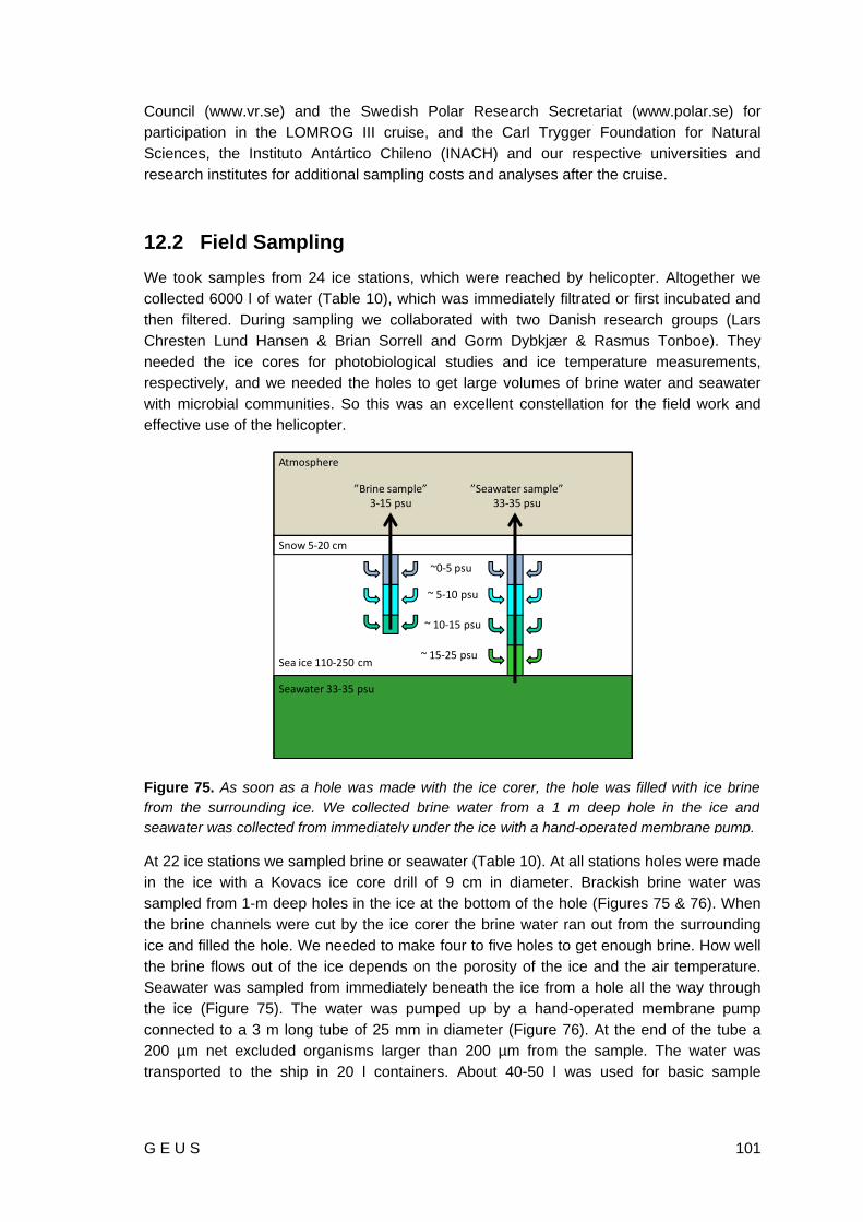
G E U S 101

Council (www.vr.se) and the Swedish Polar Research Secretariat (www.polar.se) for participation in the LOMROG III cruise, and the Carl Trygger Foundation for Natural Sciences, the Instituto Antártico Chileno (INACH) and our respective universities and research institutes for additional sampling costs and analyses after the cruise.

12.2 Field Sampling We took samples from 24 ice stations, which were reached by helicopter. Altogether we collected 6000 l of water (Table 10), which was immediately filtrated or first incubated and then filtered. During sampling we collaborated with two Danish research groups (Lars Chresten Lund Hansen & Brian Sorrell and Gorm Dybkjær & Rasmus Tonboe). They needed the ice cores for photobiological studies and ice temperature measurements, respectively, and we needed the holes to get large volumes of brine water and seawater with microbial communities. So this was an excellent constellation for the field work and effective use of the helicopter.

At 22 ice stations we sampled brine or seawater (Table 10). At all stations holes were made in the ice with a Kovacs ice core drill of 9 cm in diameter. Brackish brine water was sampled from 1-m deep holes in the ice at the bottom of the hole (Figures 75 & 76). When the brine channels were cut by the ice corer the brine water ran out from the surrounding ice and filled the hole. We needed to make four to five holes to get enough brine. How well the brine flows out of the ice depends on the porosity of the ice and the air temperature. Seawater was sampled from immediately beneath the ice from a hole all the way through the ice (Figure 75). The water was pumped up by a hand-operated membrane pump connected to a 3 m long tube of 25 mm in diameter (Figure 76). At the end of the tube a 200 µm net excluded organisms larger than 200 µm from the sample. The water was transported to the ship in 20 l containers. About 40-50 l was used for basic sample

Figure 75. As soon as a hole was made with the ice corer, the hole was filled with ice brinefrom the surrounding ice. We collected brine water from a 1 m deep hole in the ice andseawater was collected from immediately under the ice with a hand-operated membrane pump.

Snow 5‐20 cm

Seawater 33‐35 psu

~0‐5 psu

~ 5‐10 psu

~ 10‐15 psu

~ 15‐25 psu

”Brine sample” 3‐15 psu

”Seawater sample” 33‐35 psu

Sea ice 110‐250 cm

Atmosphere

102 G E U S

characteristics, 10-20 l for DNA and RNA samples, 90-150 l for metagenomics, and 80-100 l for incubation experiments. We also took triplicate 40 or 80 ml water samples of for NH4 analyses.

At 6 ice stations we took samples of both the upper meter brine water and the upper meter ice core to compare the biomass and the species composition in the brine and that of the part of the microbial community that was left in the ice core. The ice cores were transported to the ship in previously ethanol-disinfected polycarbonate boxes and left to melt in these boxes which took ca. 70 hours (Table 10; Figure 76).

At 12 CTD stations we collected water samples from the rosette to study the distribution of compounds involved in microbial processes (N2O, CH4, DMSP) in the water column (Tables 11 & 12; Figure 77).

All stations are shown in a map in Figure 78.

Table 10. Ice stations of the microbial group during LOMROG III.

Ice station Seawater Brine water Ice core Lab Field water Ice depth Snow depth

Date Time Position N Position E/W nr L L length cm salinity temp °C m cm

03/08/2012 09:30 ‐ 13:00 N 84o 09.604' E 014o 57.893' 1 0 280 0 15 ‐0.9 2.5 15

04/08/2012 09:15 ‐ 12:30 N 85o 18.630' E 006o 47.397' 2 0 280 0 15 ‐0.6 1.6 20

06/08/2012 09:00 ‐ 12:00 N 86o 51.906' E 000o 12.612' 3 280 0 0 34.9 ‐1.6 1.5 10

07/08/2012 12:30 ‐ 15:00 N 87o 03.820' W 006o 46.669' 4 280 0 0 34.7 ‐1.5 1.5 7.5

09/08/2012 09:00 ‐ 12:30 N 87o 45.130' W 034o 41.960' 5 0 280 0 15 ‐1.0 1.5 5

10/08/2012 09:00 ‐ 12:00 N 87o 47.304' W 042o 31.823' 6 280 0 0 33.7 ‐1.4 1.5 10

12/08/2012 09:10 ‐ 12:00 N 87o 50.742' W 059o 38.684' 7 0 280 0 6 ‐0.5 1.3 5

13/08/2012 09:30 ‐ 12:30 N 88o 11.745' W 053o 35.926' 8 0 280 0 9 ‐0.5 1.5 5

15/08/2012 09:00 ‐ 11:30 N 88o 11.744' W 049o 33.588' 9 280 0 0 33.1 ‐1.4 1.6 5

17/08/2012 13:00 ‐ 16:00 N 88o 19.509' W 066o 44.409' 10 0 280 0 5 ‐0.5 1.5 3

19/08/2012 19:30 ‐ 22:00 N 89o 11.388' W 070o 50.089' 11 280 0 0 33.3 ‐1.5 1.5 10

21/08/2012 15:00 ‐ 18:00 N 89o 56.112' W 073o 41.687' 12 0 280 0 9 ‐0.5 1.5 10

23/08/2012 10:00 ‐ 13:00 N 89o 50.322' E 135o 55.486' 13 280 0 0 34.0 ‐1.5 1.2 10

25/08/2012 13:30 ‐ 16:00 N 87o 58.544' E 122o 09.066' 14 0 280 0 2.5 ‐0.5 1.6 15

28/08/2012 16:00 ‐ 18:30 N 87o 56.546' E 073o 29.387' 15 0 280 0 7 ‐0.5 1.6 20

29/08/2012 15:00 ‐ 18:00 N 88o 15.639' E 072o 51.762' 16 0 20 150 9.6 ‐0.5 1.5 15

30/08/2012 13:30 ‐ 16:00 N 88o 27.286' E 068o 26.976' 17 200 40 400 35.2 / 5 ‐1.4 1.1 20

31/08/2012 09:00 ‐ 12:30 N 88o 42.748' E 055o 56.346' 18 0 40 425 3.2 ‐0.5 1.6 12

02/09/2012 09:00 ‐ 12:00 N 88o 28.188' E 022o 18.720' 19 0 240 400 19 ‐0.8 1.7 5

03/09/2012 14:00 ‐ 17:00 N 88o 24.303' E 023o 50.964' 20 240 0 0 34.9 ‐1.4 1.6 5

04/09/2012 16:00 ‐ 19:00 N 87o 44.353' E 030o 05.521' 21 0 240 410 5.2 ‐0.6 1.4 7.5

05/09/2012 14:30 ‐ 17:00 N 87o 35.896' E 020o 32.982' 22 260 0 0 35.0 ‐1.7 2.2 7.5

07/09/2012 08:30 ‐ 11:30 N 85o 25.653' E 005o 15.952' 23 0 260 415 4.5 ‐0.6 1.5 7.5

09/09/2012 09:00 ‐ 11:30 N 83o 49.449' E 015o 08.015' 24 260 0 0 34.8 ‐1.7 1.1 10

Sum 2640 3360 2200

G E U S 103

Table 11. CTD stations of the microbial group during LOMROG III.

Date Time Position N Position E/W CTD station02/08/2012 11:35 N 82o 57.48' E 014o 55.98' 1

05/08/2012 17:03 N 86o 44.59' E 001o 57.31' 2

09/08/2012 13:09 N 87o 46.20' W 037o 45.45' 3

16/08/2012 05:10 N 88o 20.80' W 069o 24.69' 4

20/08/2012 05:10 N 89o 15.90' W 058o 50.83' 5

27/08/2012 11.21 N 88o 08.96' E 078o 14.56' 6

31/08/2012 13:56 N 88o 47.43' E 053o 06.18' 7

07/09/2012 06:44 N 85o 25.59' E 005o 16.63' 8

08/09/2012 07:36 N 84o 22.21' E 003o 43.29' 9

09/09/2012 06:46 N 83o 49.41' E 015o 10.37' 10

10/09/2012 06:23 N 82o 46.12' E 014o 44.67' 11

11/09/2012 06:16 N 82o 11.75' E 008o 45.12' 12

Figure 76. As soon as a hole was made with the ice corer, the hole was filled with ice brinefrom the surrounding ice. We collected brine water from a 1 m deep hole in the ice andseawater was collected from immediately under the ice with a hand-operated membrane pump.At some sites also the ice core was sampled and melted in the lab (Upper photograph by LarsChresten Lund Hansen).

104 G E U S

Table 12. Sampling depths of the CTD stations. All depths were sampled for N2O and CH4 and the depths indicated in blue were sampled for DMSP.

Depth Depth Depth Depth Depth Depth Depth Depth Depth Depth Depth Depth Depth Depth Depth Depth Depth

CTD station m m m m m m m m m m m m m m m m m

1 10 20 40 60 100 150 200 500 1000 1500 2000 2500

2 10 20 40 60 100 150 200 500 1000 1500 2000 2500

3 10 20 40 60 100 200 500 1000 1500 2000 3000 3500

4 10 20 40 60 100 200 500 1000 1200

5 10 20 40 60 100 200 500 1000 1500 2000 3000 3743

6 10 20 40 60 100 200 500 1000 1500 2500 3000 3353

7 10 20 40 60 100 200 500 1000 1500 2000 2500 3000 3500 4000 4460

8 10 20 40 60 100 200 500 1000 1500 2000 2500 3000

9 10 20 40 60 100 200 500 1000 1500 2000 2500 3000 3778

10 10 20 40 60 100 200 500 1000 1500 2000 2500 3000 3500 4000

11 10 20 40 60 100 200 300 500 1000 1451

12 10 20 40 60 100 200 300 500 1000 1451

Figure 77. Sampling from the CTD for the analysis of N2O, CH4 and DMSP in water columnprofiles.

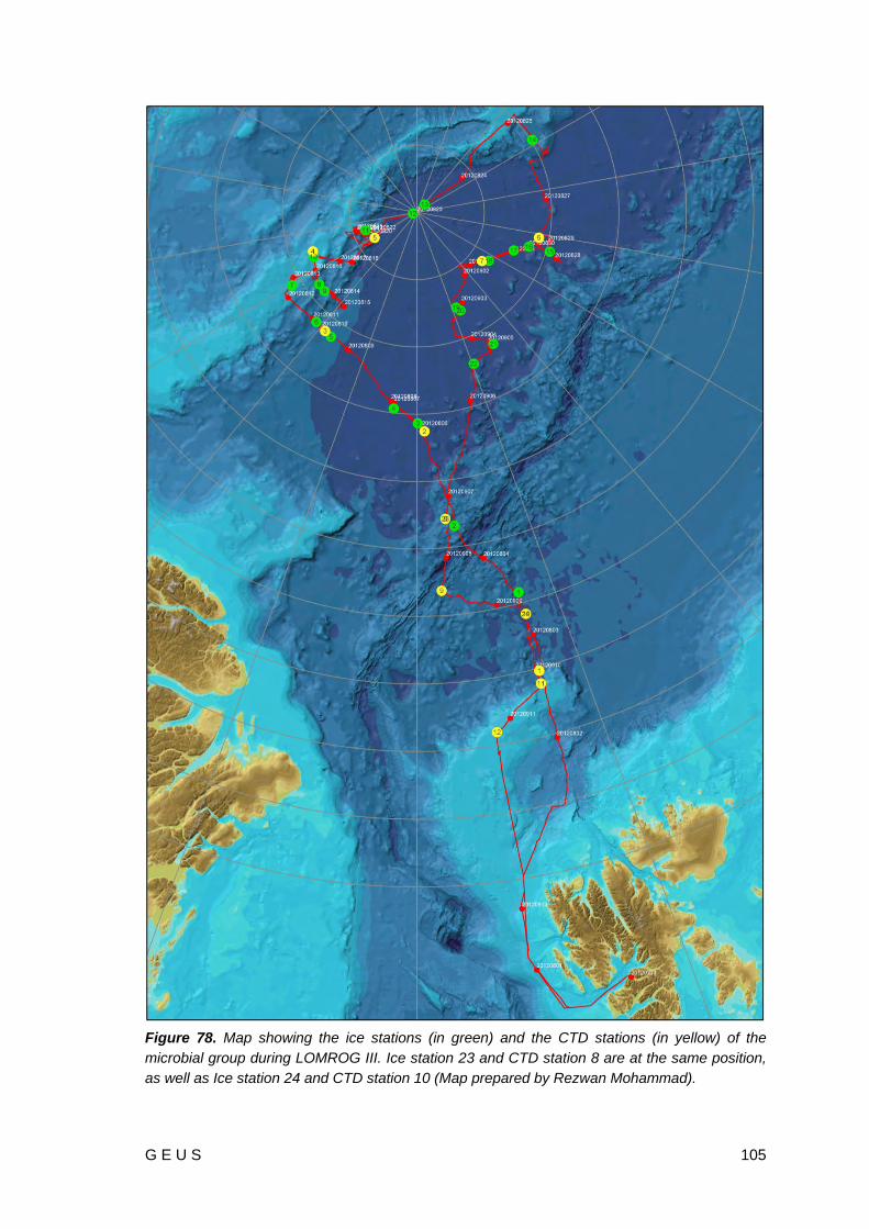
G E U S 105

Figure 78. Map showing the ice stations (in green) and the CTD stations (in yellow) of the microbial group during LOMROG III. Ice station 23 and CTD station 8 are at the same position, as well as Ice station 24 and CTD station 10 (Map prepared by Rezwan Mohammad).

106 G E U S

12.3 Basic sample characteristics

12.3.1 Water Temperature and Salinity

Water temperature and salinity were measured with an YSI Pro30 handheld conductivity meter during field sampling. Salinity was measured again in the laboratory before the water was filtered.

12.3.2 Inorganic Nutrient Concentrations in the Water

The concentrations of NH4 in the water were measured directly on board with a Perkin Elmer LS 55 Fluorescence Spectrometer according to the method of Holmes et al. (1999) with incubation time extended to 12 hours. The NH4 concentrations varied between below detection level (ca. 5 nM) and 290 nM (Figure 79). The highest concentrations were found in the brine where the NH4 concentrations showed the highest variation. For analyses of NO3, NO2, PO4 and SiO2 concentrations four replicate 12 ml water samples per sampling station were filtered over a 0.45 µm membrane filter and frozen at -20ºC for later analysis at Stockholm University.

12.3.3 DOC and Isotopic Composition of O and H in Water and of C and N in Particulate Matter

For DOC analysis a water volume of 40 ml was fixed with HgCl2 and stored in dark bottles at 4ºC. For the isotopic composition of hydrogen and oxygen water volumes of 15 ml were taken in Falcon tubes and stored at 4ºC. For the analysis of POC and PON and their isotopic composition (δ13C and δ15N), particulate matter >0.7 µm was filtered on pre-combusted GF/F filters (Table 13, Figure 80) and are stored at -80ºC. These samples are will be analyzed at the Universidad de Concepción (δ13C and δ15N in t=0 samples of the experiments) and at CSIC (O, H, δ13C and δ15N in field samples).

Figure 79. Results of the on-board NH4 measurements. Blue = brine, green = seawater.

0

50

100

150

200

250

300

350NH4 concentration (nM)

G E U S 107

12.3.4 Cell Size and Density

For flow cytometry a water volume of 5 ml was fixed with glutaraldehyde (1.0%) onboard and stored at 4ºC (Table 13). These samples will be analysed at the Universidad de Concepción.

12.3.5 Verification of Viable Cells

To check the viability of the cells and record the dominant algal species, ca. 1 l of water was filtered on a 45 mm 0.2 µm membrane filter and observed under a light microscope on-board. Small subsamples were also taken from selected metagenomics filters. Both types of samples were fixed with glutaraldehyde (2.5%) in an Eppendorf tube onboard and stored at 4ºC. The verification of viable bacterial cells (including phototrophs) in the samples will be performed by optical and epifluorescence light microscopy staining with DAPI and acridine orange (Hobbie et al. 1977). These samples will be analysed at the Universidad Católica de Chile.

12.3.6 Fluorescence and Photosynthetic Performance

The photosynthetic properties of all water sampled were analysed with a PhytoPAM Phytoplankton analyser, Model Phyto US, Walz, Germany (Figure 81). Measurements included maximum fluorescence (Fm), which can be interpreted as a measure of biomass, photosynthetic yield (Fv/Fm), a measure of photosynthetic capacity. PI-curves were made as well to assess the initial rate of photosynthesis (), light compensation point (Ik) and electron transport rate (ETR). The data will be further calculated at the University of Stockholm.

12.3.7 Pigments

For HPLC analysis of chlorophylls (a,b,c) and ca. 20 carotenoids, particulate matter >0.7 µm was filtered on pre-combusted GF/F filters (Table 13, Figure 80) and are stored at -80⁰C. These samples will be analysed at the University of Stockholm.

108 G E U S

Figure 81. The PhytoPAM Phytoplankton analyzer PhytoPAM Phytoplankton Analyzer, ModelPhyto US (Walz, Germany) used for measuring fluorescence and photosynthetic performanceduring the cruise.

Figure 80. Equipment used for filtering microbial communities on GF/F filters Upper filter =seawater from Ice station 20, lower filter = brine from Ice station 23.

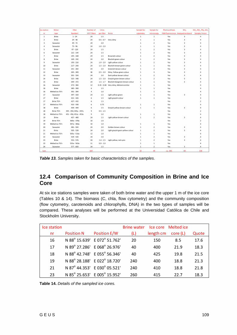
G E U S 109

Table 13. Samples taken for basic characteristics of the samples.

12.4 Comparison of Community Composition in Brine and Ice Core At six ice stations samples were taken of both brine water and the upper 1 m of the ice core (Tables 10 & 14). The biomass (C, chla, flow cytometry) and the community composition (flow cytometry, carotenoids and chlorophylls, DNA) in the two types of samples will be compared. These analyses will be performed at the Universidad Católica de Chile and Stockholm University.

Table 14. Details of the sampled ice cores.

Ice station Water Filter Number of Litres Sample for Sample for Photosynthesis NH4 NO3, NO2, PO4, SiO2

nr type Numbers GF/F filters per filter Notes cytometry microscopy PAM fluorescence Analyzed on board Samples frozen

1 Brine 1 ‐ 24 24 1.5 1 1 Yes 3 4

2 Brine 24 ‐ 48 24 0.5 ‐ 0.7 Very slimy 1 1 Yes 3 4

3 Seawater 49 ‐ 72 24 2.0 1 2 Yes 3 4

4 Seawater 73 ‐ 96 24 1.0 ‐ 2.0 1 1 Yes 3 4

5 Brine 97 ‐ 120 24 1.5 1 2 Yes 3 4

6 Seawater 121 ‐ 144 24 1.5 1 2 Yes 3 4

7 Brine 145 ‐ 168 24 1.5 Brownish colour 1 2 Yes 3 4

8 Brine 169 ‐ 192 24 2.0 Blackish green colour 1 2 Yes 3 4

9 Seawater 193 ‐ 216 24 1.9 ‐ 2.0 Light yellow colour 1 2 Yes 3 4

10 Brine 217 ‐ 240 24 1.5 ‐ 2.0 Blackish brown‐green colour 1 1 Yes 3 4

11 Seawater 241 ‐ 264 24 2.0 Greenish‐brown colour 1 2 Yes 3 4

12 Brine 265 ‐ 300 36 0.5 ‐ 2.0 Slimy, Yellow‐green colour 1 3 Yes 3 4

13 Seawater 301 ‐ 324 24 2.0 Dark yellow‐brown colour 1 2 Yes 3 4

14 Brine 325 ‐ 348 24 1.5 ‐ 2.0 Greyish green‐brown colour 1 2 Yes 3 4

15 Brine 349 ‐ 372 24 1.5 ‐ 1.7 Blackish bluegreen‐brown colour 1 1 Yes 3 4

16 Seawater 373 ‐ 384 12 0.35 ‐ 0.48 Very slimy, Melosira arctica 1 1 Yes 4

16 Brine 385 ‐ 390 6 1.5 1 1 Yes 4

16 Melted ice 70 h 391 ‐ 394 4 1.0 1 1 Yes 4

17 Seawater 397 ‐ 420 24 1.5 Light yellow‐green 1 1 Yes 3 4

17 Brine 421 ‐ 426 6 1.5 Light greyish colour 1 1 Yes 4

17 Brine 70 h 427 ‐ 432 6 1.5 Yes 2

17 Melted ice 70 h 433 ‐ 438 6 0.75 1 1 Yes 4

18 Brine 439 ‐ 444 6 1.5 Greyish yellow‐brown colour 1 1 Yes 3 4

18 Brine 70 h 445 ‐ 450, 445a ‐ 447a 9 0.5 ‐ 1.5 Yes 2

18 Melted ice 70 h 451 ‐ 456, 451a ‐ 453a 9 1.0 1 1 Yes 4

19 Brine 457 ‐ 480 24 1.5 Light yellow‐brown colour 1 2 Yes 3 4

19 Brine 70 h 469a ‐ 478a 10 1.0 Yes 2

19 Melted ice 70 h 457a ‐ 466a 10 1.0 1 1 Yes 4

20 Seawater 481 ‐ 504 24 2.0 Golden‐brown colour 1 2 Yes 3 4

21 Brine 505 ‐ 528 24 2.0 Light greyish geen‐yellow colour 1 2 Yes 3 4

21 Melted ice 70 h 505a ‐ 516a 12 1.0 1 1 Yes 4

22 Seawater 529 ‐ 534 24 2.0 1 2 Yes 3 4

23 Brine 553 ‐ 576 24 1.4 ‐ 1.5 Light yellow, red cysts 1 2 Yes 3 4

23 Melted ice 70 h 553a ‐ 563a 11 0.9 ‐ 1.0 1 1 Yes 4

24 Seawater 577 ‐ 600 24 1.5 1 2 Yes 3 4

Sum 647 32 49 ca. 200 69 134

Ice station Brine water Ice core Melted icenr Position N Position E/W (L) length cm core (L) Quote

16 N 88o 15.639' E 072o 51.762' 20 150 8.5 17.6

17 N 89o 27.286' E 068o 26.976' 40 400 21.9 18.3

18 N 88o 42.748' E 055o 56.346' 40 425 19.8 21.5

19 N 88o 28.188' E 022o 18.720' 240 400 18.8 21.3

21 N 87o 44.353' E 030o 05.521' 240 410 18.8 21.8

23 N 85o 25.653' E 005o 15.952' 260 415 22.7 18.3

110 G E U S

12.5 CTD samples

12.5.1 N2O and CH4

Altogether 572 samples (134 station/depths) were taken from the CTD for the analysis of the gases N2O and CH4 in the seawater column. Duplicate water samples of 20 ml were collected in GC gas-tight vials for each of the gases, preserved with 50 µl saturated HgCl2 and stored at room temperature (ca. 20ºC) in the dark. These samples will be analyzed at the Universidad de Concepción.

12.5.2 DMSP

Altogether 120 samples (60 station/depths) were taken from the CTD for the analysis of dimethylsulfoniopriopionate (DMSP) in the seawater column. Only the upper 100 m was sampled as this is gas is produced by algae. Duplicate water samples of 20 ml were collected in GC gas-tight vials, preserved with 50 µl 50% sulphuric acid and stored at room temperature (ca. 20ºC) in the dark. These samples will be analysed at the AWI in Bremerhaven.

12.6 Molecular Field Samples

12.6.1 RNA Field Samples

In the field one 20-L container was filled immediately before the helicopter lifted from the ice. It reached the laboratory within 20-30 minutes during it was kept at 0ºC and was immediately filtered for RNA analyses. For this, 2.5 - 4 l were sequentially filtered (Figure 80) on 45 mm 20 µm Millipore nylon filters, 45 mm 8 µm Millipore polycarbonate filters and 0.2 µm Millipore Sterivex filters using a Cole Palmer System peristaltic pump Model No 7553-70 (6-600 rpm). This was done in duplicate. The six RNA filters were preserved in RNAlater and stored at -80ºC (Table 15). The samples will be analysed at the Universidad Católica de Chile. They will be extracted using commercial kits, and PCR amplification will be performed for nifH gene analyses of the active diastrophic community. The nifH gene fragments present in each sample will be resolved and compared by the DGGE fingerprinting technique and clone libraries. All DGGE bands and clones will be sequenced and the identity and the relative abundance of the active diastrophic community will be obtained for each station. Q-PCR will be also performed to obtain and compare the quantitative abundances of diastrophic organisms present in the samples.

G E U S 111

12.6.2 DNA Field Samples

From the same container as used for the RNA samples, 5-11 l were sequentially filtered (Figure 82) on 45 mm 20 µm Millipore nylon filters, 45 mm 8 µm Millipore polycarbonate filters and 0.2 µm Millipore Sterivex filters using a Cole Palmer System peristaltic pump Model No 7553-70 (6-600 rpm). The three DNA filters were stored at -80ºC (Table 15). The samples will be analysed at the Universidad Católica de Chile. They will be extracted following standard protocols and PCR amplification will be performed for the 16S rRNA and nifH genes of the prokaryotic community. These gene fragments present in each sample will be resolved and compared by the DGGE fingerprinting technique and clone libraries. In addition, 16S tag sequencing with Solexa technology will be performed at MIT (Boston) for all samples to study the diversity and relative abundances of the taxa in the prokaryotic community at each station in more detail.

12.6.3 Metagenomics Field Samples

One sample for DNA/RNA metagenomics/transcriptomic analysis was collected at each station. Between 90 and 150 l were sequentially filtered (Figure 82) on 293 mm Millipore Supor filters of 3 µm, 0.8 µm and 0.1 µm pore size, respectively, with the help of an air pump (Flojet industrial air pump Model G575215) and a compressor (Meec tools, 2Hp 50 L, 10 bar). The air pressure was kept below 5 Bar and 50 PSI. After filtration the filters were put in 50 mL sterile Falcon tubes and 200 µL TE buffer, 400 µl EDTA, 400 µl EGTA, 10 ml of RNAlater and 10 ml of molecular water. The tubes were stored at -80ºC (Table 615). DNA/RNA will be extracted from the samples following standard protocols at the Venter Institute (SanDiego), and then sequenced by 454-technology for meta-genomic/transcriptomic analysis in San Diego or Stockholm Genomic Centre in the Karolinska Institute.

Table 15. Details of the RNA, DNA and metagenomics samples. * = 55 µm filters were used for the RNA and DNA samples instead of 20 µm filters, ** = extra samples taken for RNA and DNA, * = 12 µm filters were used for the RNA and DNA samples instead of 8 µm filters, **** = 45 mm 0.2 µm filters were used instead of Sterivex filters.

Ice station Water RNA1 RNA1 RNA1 RNA2 RNA2 RNA2 DNA DNA DNA Metagenome Metagenome Metagenome

nr type 20‐200 µm 8‐20 µm 0.2‐8 µm 20‐200 µm 8‐20 µm 0.2‐8 µm 55‐200 µm 8‐55 µm 0.2‐8 µm 3‐200 µm 0.8‐3 µm 0.1‐0.8 µm Note

1 Brine 2.6 2.6 2.6 3.0 3.0 3.0 12.0 12.0 12.0 140 140 140 *

2 Brine 2.8 2.8 2.8 3.0 3.0 3.0 6.0 6.0 6.0 70 70 70 *

3 Seawater 3.2 3.2 3.2 3.6 3.6 3.6 16.5 16.5 16.5 110 110 110

4 Seawater 4.0 4.0 4.0 4.1 4.1 4.1 12.5 12.5 12.5 130 130 130

5 Brine 3.4 3.4 3.4 2.9 2.9 2.9 10.0 10.0 10.0 120 120 120

6 Seawater 2.7 2.7 2.7 3.2 3.2 3.2 18.5 18.5 18.5 110 110 110

7 Brine 2.5 2.5 2.5 2.1 2.1 2.1 5.0 5.0 5.0 120 120 120

8 Brine 4.1 4.1 4.1 4.0 4.0 4.0 10.0 10.0 10.0 100 100 100

9 Seawater 3.2 3.2 3.2 2.7 2.7 2.7 16.0 16.0 16.0 110 110 110

10 Brine 2.6 2.6 2.6 2.1 2.1 2.1 8.0 8.0 8.0 130 130 130

11 Seawater 3.6 3.6 3.6 3.1 3.1 3.1 14.0 14.0 14.0 150 150 150

12 Brine 3.0 3.0 3.0 3.0 3.0 3.0 1.0 1.0 1.0 130 130 130 **

13 Seawater 2.2 2.2 2.2 2.5 2.5 2.5 7.0 7.0 7.0 90 90 90

14 Brine 2.3 2.3 2.3 2.6 2.6 2.6 7.0 7.0 7.0 100 100 100

15 Brine 3.0 3.0 3.0 3.1 3.1 3.1 8.0 8.0 8.0 100 100 100

16 Seawater 1.4 1.4 1.4 2.4 2.4 2.4 ***

16 Brine 3.2 3.2 3.2 7.5 7.5 7.5

17 Seawater 3.4 3.4 3.4 3.2 3.2 3.2 11.0 11.0 11.0 140 140 140

17 Brine 3.2 3.2 3.2 3.0 3.0 3.0 9.0 9.0 9.0

17 Melted ice 70 h 6.0 6.0 6.0

18 Brine 3.0 3.0 3.0 3.1 3.1 3.1 8.0 8.0 8.0

18 Melted ice 70 h 5.4 5.4 5.4

19 Brine 2.4 2.4 2.4 3.0 3.0 3.0 7.0 7.0 7.0 160 160 160

19 Melted ice 70 h 6.0 6.0 6.0

20 Seawater 3.1 3.1 3.1 3.5 3.5 3.5 12.0 12.0 12.0 160 160 160

21 Brine 3 3 3 3 3 3 8.0 8.0 8.0 140 140 140

21 Melted ice 70 h 6.0 6.0 6.0

22 Seawater 3.5 3.5 3.5 4 4 4 15.0 15.0 15.0 160 160 160

23 Brine 3 3 3 3 3 3 7.5 7.5 7.5 110 110 110

23 Melted ice 70 h 4.5 4.5 4.5

24 Seawater 1.6 1.6 1.6 2 2 2 3.0 3.0 3.0 160 160 160 ****

Number of filters 26 26 26 24 24 24 31 31 31 22 22 22

112 G E U S

Figure 82. Filtration of the molecular samples on different types of filters.

12.7 Biogeochemical Experiments with Stable Isotopes Eleven experiments were carried out, seven with brine and four with seawater (Table 16). In these experiments different C and N tracers were added in order to measure a wide spectrum of biogeochemical processes occurring in seawater and brine. Regarding N metabolisms, phototrophic and heterotrophic N2 fixation was measured under bicarbonate or glucose additions, respectively. In addition, nitrate and ammonium uptake along with bicarbonate uptake were assayed with samples incubated under light and dark condition. Thus, with these experimental setup, photo (light C assimilation) and chemolithotrophic (dark C assimilation) activities can be determined. Finally, N2O fixation (15N2O additions) was assayed as an alternative and not yet well studied substrate for N2 fixation.

To achieve this, water (brine or seawater) samples were incubated with different stable isotopes in a refrigerator with glass doors and illumination outside (Figure 83), filtered on pre-combusted GF/F filters and frozen at -20ºC. The incubations with 15N2 (3 ml of 99% 15N2) and 15N2O (1 ml of 99% 15N2O) were carried out in gas-tight flasks of 2.75 l, while for the incubations with 15NO3 (20-80 µl of 500 µM NO3

-) and 15NH4 (20 µl of 500 µM 15NH4+)

were carried out in gas-tight flasks of 0.58 l.

However, when 15NO3 and 15NH4 incubations were carried out in conjunction with RNA expression (see section 12.9) these were also carried out in the larger flasks (2.75 l). The zero samples (without isotopes), the incubations with 15N2 and 15N2O (gases) and with 15NO3 and 15NH4 were performed in three different labs to avoid potential contamination. These samples will be analysed at the Universidad de Concepción. During the last day of experiments extra filters were taken for inter-calibration between the laboratories in Concepción and Bremen.

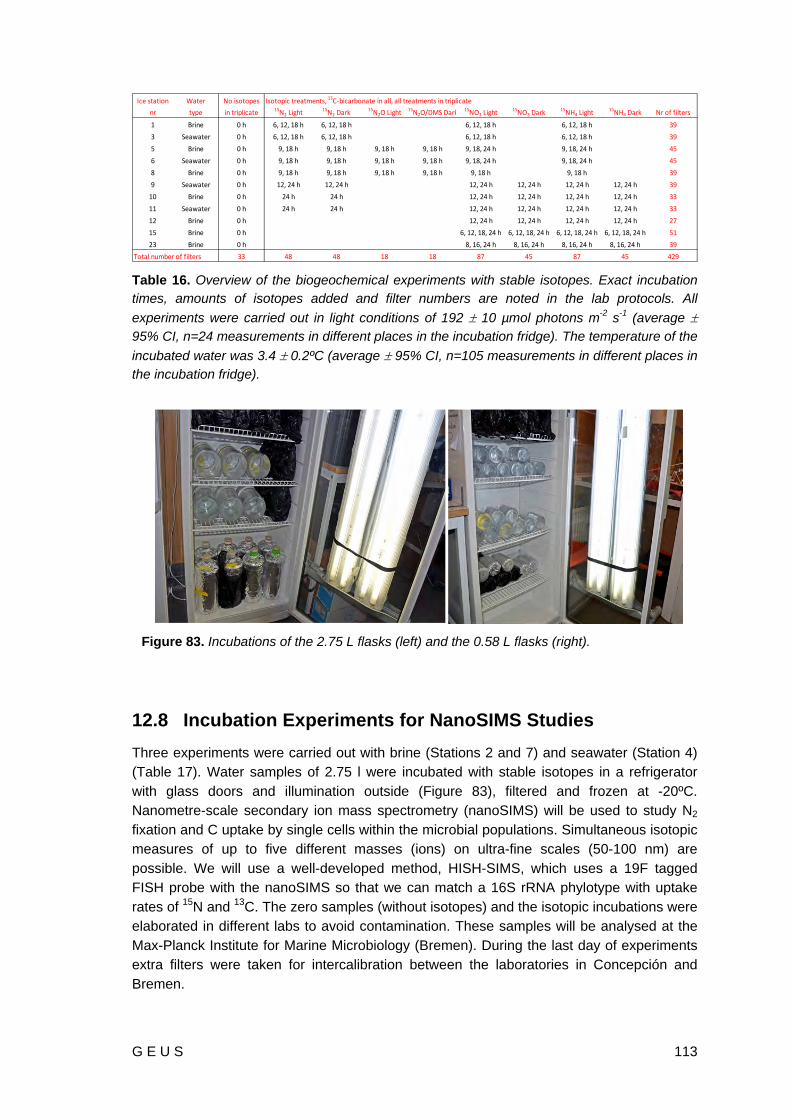
G E U S 113

Table 16. Overview of the biogeochemical experiments with stable isotopes. Exact incubation times, amounts of isotopes added and filter numbers are noted in the lab protocols. All

experiments were carried out in light conditions of 192 10 µmol photons m-2 s-1 (average 95% CI, n=24 measurements in different places in the incubation fridge). The temperature of the

incubated water was 3.4 0.2ºC (average 95% CI, n=105 measurements in different places in the incubation fridge).

12.8 Incubation Experiments for NanoSIMS Studies Three experiments were carried out with brine (Stations 2 and 7) and seawater (Station 4) (Table 17). Water samples of 2.75 l were incubated with stable isotopes in a refrigerator with glass doors and illumination outside (Figure 83), filtered and frozen at -20ºC. Nanometre-scale secondary ion mass spectrometry (nanoSIMS) will be used to study N2 fixation and C uptake by single cells within the microbial populations. Simultaneous isotopic measures of up to five different masses (ions) on ultra-fine scales (50-100 nm) are possible. We will use a well-developed method, HISH-SIMS, which uses a 19F tagged FISH probe with the nanoSIMS so that we can match a 16S rRNA phylotype with uptake rates of 15N and 13C. The zero samples (without isotopes) and the isotopic incubations were elaborated in different labs to avoid contamination. These samples will be analysed at the Max-Planck Institute for Marine Microbiology (Bremen). During the last day of experiments extra filters were taken for intercalibration between the laboratories in Concepción and Bremen.

Ice station Water No isotopes Isotopic treatments, 13C‐bicarbonate in all, all treatments in triplicatenr type in triplicate 15N2 Light

15N2 Dark15N2O Light

15N2O/DMS Dark 15NO3 Light15NO3 Dark

15NH4 Light15NH4 Dark Nr of filters

1 Brine 0 h 6, 12, 18 h 6, 12, 18 h 6, 12, 18 h 6, 12, 18 h 39

3 Seawater 0 h 6, 12, 18 h 6, 12, 18 h 6, 12, 18 h 6, 12, 18 h 39

5 Brine 0 h 9, 18 h 9, 18 h 9, 18 h 9, 18 h 9, 18, 24 h 9, 18, 24 h 45

6 Seawater 0 h 9, 18 h 9, 18 h 9, 18 h 9, 18 h 9, 18, 24 h 9, 18, 24 h 45

8 Brine 0 h 9, 18 h 9, 18 h 9, 18 h 9, 18 h 9, 18 h 9, 18 h 39

9 Seawater 0 h 12, 24 h 12, 24 h 12, 24 h 12, 24 h 12, 24 h 12, 24 h 39

10 Brine 0 h 24 h 24 h 12, 24 h 12, 24 h 12, 24 h 12, 24 h 33

11 Seawater 0 h 24 h 24 h 12, 24 h 12, 24 h 12, 24 h 12, 24 h 33

12 Brine 0 h 12, 24 h 12, 24 h 12, 24 h 12, 24 h 27

15 Brine 0 h 6, 12, 18, 24 h 6, 12, 18, 24 h 6, 12, 18, 24 h 6, 12, 18, 24 h 51

23 Brine 0 h 8, 16, 24 h 8, 16, 24 h 8, 16, 24 h 8, 16, 24 h 39

Total number of filters 33 48 48 18 18 87 45 87 45 429

Figure 83. Incubations of the 2.75 L flasks (left) and the 0.58 L flasks (right).

114 G E U S

Table 17. Basic set-up of the three nanoSIMS experiments (Stations 2, 4 and 7). Exact incubation times and filter numbers are noted in the lab protocols. The isotopic additions were 3 ml of 15N2-gas, 500 µl of 500 mM 13C-bicarbonate and 70 µl of 100 mM 13C-bicarbonate. All

experiments were carried out in light conditions of 192 10 µmol photons m-2 s-1 (average 95% CI, n=24 measurements in different places in the incubation fridge), except for Station 2 when the glucose treatment was in the dark (wrapped in aluminium foil). The temperature of the

incubated water was 3.4 0.2ºC (average 95% CI, n=105 measurements in different places in the incubation fridge).

12.9 Diurnal RNA Expression Four experiments were performed to analyse diurnal RNA expression in seawater and ice brine communities (Table 18). Water samples were incubated in gas-tight flasks of 2.75 l with and without stable isotopes, and with and without illumination, in a refrigerator with glass doors and illumination outside (Figure 83). These experiments were carried out in conjunction with the incubation experiments summarized in Table 16. The different treatments included no additions of isotopes and additions of 15N2, 15NO3 and 15NH4 (Table 18). After different incubation times the samples were sequentially filtered (Figure 82) on 45 mm 20 µm Millipore nylon filters, 45 mm 8 µm Millipore polycarbonate filters and 0.2 µm Millipore Sterivex filters using a Cole Palmer System peristaltic pump Model No 7553-70 (6-600 rpm). The filters were preserved in RNAlater and stored at -80ºC.

These samples will be analysed at the Universidad Católica de Chile. RNA will be extracted from the samples using commercial kits and Q-PCR analysis will be performed for nifH gene quantifications of the diastrophic community activity with time, as well as other genes involved in the combined nitrogen uptake. The RNA expression will be compared with the N2 fixation and DIN uptake rates, which were measured simultaneously (Table 16).

Bulk nanoSIMS nanoSIMS Treatment Time on pre‐combusted GF/F filters on gold‐coated 3 µm filters on gold‐coated 0.2 µm filters

No isotopes 0 h 3 x 2.20 L 1 x 2.75 L 1 x 2.75 L

15N2‐gas +13C‐bicarb 6 h 3 x 2.75 L 1 x 2.75 L 1 x 2.75 L



15N2‐gas +13C‐glucose 6 h 3 x 2.75 L 1 x 2.75 L



Total nr of filters 21 filters 4 filters 7 filters

G E U S 115

Table 18. Overview of the RNA-expression experiments. Exact incubation times, amounts of isotopes added and filter numbers are noted in the lab protocols. All experiments were carried

out in light conditions of 192 10 µmol photons m-2 s-1 (average 95% CI, n=24 measurements

in different places in the incubation fridge). The temperature of the incubated water was 3.4

0.2ºC (average 95% CI, n=105 measurements in different places in the incubation fridge).

12.10 References Díez, B., Bergman, B., Pedrós-Allio, C., Antó, M. & Snoeijs, P. 2012: High cyanobacterial

nifH gene diversity in Arctic seawater and sea ice brine. Environmental Microbiology Reports, doi:10.1111/j.1758-2229.2012.00343.x.

Bowman, J.S., Rasmussen, S., Blom, N., Deming, J.W., Rysgaard, S. & Sicheritz-Ponten, T. 2012: Microbial structure of Arctic multiyear sea ice and surface seawater by 454 sequencing of the 16S RNA gene. The ISME Journal 6, 11-20.

Holmes, R. M., Aminot, A., Kérouel, R., Hooker, B. A., Peterson, B. J. 1999: A simple and precise method for measuring ammonium in marine and freshwater ecosystems. Canadian Journal of Fisheries and Aquatic Sciences 56, 1801-1808.

Hobbie, J. E., Daley, R. H., Jasper, S. 1977: Use of Nuclepore filters for counting bacteria by fluorescence microscopy. Applied and Environmental Microbiology 33, 1225-1228.

Ice station Water No isotopes No isotopes No isotopes Isotopic treatments, 13C‐bicarbonate in all, all treatments in triplicate

nr type in duplicate Light Dark 15N2 Light15N2 Dark

15NO3 Light15NO3 Dark

15NH4 Light15NH4 Dark Nr of filters

9 Seawater 0 h 12, 24 h 12, 24 h 12, 24 h 12, 24 h 12, 24 h 12, 24 h 14

13 Seawater 0 h 6, 12, 18, 24 h6, 12, 18, 24 h 6, 12, 18, 24 h6, 12, 18, 24 h 18

15 Brine 0 h 6, 12, 18, 24 h6, 12, 18, 24 h 6, 12, 18, 24 h6, 12, 18, 24 h6, 12, 18, 24 h6, 12, 18, 24 h 26

23 Brine 0 h 8, 16, 24 h 8, 16, 24 h 8, 16, 24 h 8, 16, 24 h 8, 16, 24 h 8, 16, 24 h 20

Total number of filters 8 11 11 2 2 9 9 13 13 78

116 G E U S


G E U S 117

13. Water Sampling for the Parameters of Oceanic Carbon

By Peter Sylvander, Stockholm University

Water samples were collected from one CTD station in the Amundsen basin on behalf of Ellen Druffel and Sheila Griffin, University of California, as a part of a project aiming at globally determine natural levels of 14C in dissolved organic carbon (DOC) and dissolved inorganic carbon (DIC). Sampling was performed by Peter Sylvander.

Depth (m) 4354 4000 3500 3000 2500 2000 1500 500 300 200 150 100 60 20

Table 19. Sampling depths Since 14C samples are sensitive to contamination, all surfaces equipment and bottles were in contact with were covered in clean plastic before sampling. All equipment used was cleaned and sterilized prior to departure and never handled without laboratory gloves. Equipment that by accident came into contact with a non-covered, possibly contaminated, surface was considered contaminated, discarded and replaced.

Water samples were collected from 14 depths (Table 19) using a CTD rosette operated by Steffen Olsen at CTD station LR12s06 at longitude E 78º 14.56’, latitude N88º 08.96’. To avoid contamination, the nipples of the Niskin bottles on the CTD rosette was cleaned with 10% hydrochloric acid and rinsed with MQ-water prior to sample collection. DOC-samples were collected in 1000 ml borosilicate bottles which were rinsed three times with sample water before sample collection. DOC-samples from a depth <1000 m were filtered through a GF/F filter at the time of collection from the rosette using a small filter holder attached directly to the Niskin bottles on the CTD rosette. From the same Niskin bottles, DIC-samples were collected in 500 ml polycarbonate bottles which were rinsed three times with

118 G E U S

sample water before sample collection. Since it is needed for the analyses, additional water samples for alkalinity measurements were collected in the same way as DIC-samples.

DOC-samples were stored in -20ºC after collection. DIC-samples were fixated with 50 µl HgCl2 per bottle and stored in room temperature. Alkalinity samples were stored in darkness in 4ºC. Upon de-mobilization in Helsingborg, all samples and equipment will be sent to University of California for analysis.

G E U S 119

14. Structuring of the Sea Ice Environment by Dynamic Ice-algae Activity

By Lars Chresten Lund-Hansen & Brian Sorrell, Aarhus University External Collaborators: Ian Hawes (University of Canterbury, Christchurch, New Zealand); Hans Ramløv (Roskilde University) & Erik Askov Mousing (Copenhagen University)

14.1 Introduction Photosynthesis by green plants is the basis of almost all life on earth. In the marine environment, microscopic phytoplankton are responsible most of the photosynthesis and hence plant material available to ecosystem food webs. However, the presence of sea ice greatly complicates understanding of how photosynthesis and growth function in polar vs. non-polar waters. Ice cover makes the observation and sampling of phytoplankton in the water column difficult, preventing for example the use of satellite images to monitor biomass and production, and can greatly reduce the amount of light available for photosynthesis, especially when covered by snow. Furthermore, the ice is itself colonised by algae, as liquid brine channels in the base of the ice can provide a habitat where light and nutrients are as or more plentiful than the water (Lavoie et al. 2005). The contribution of ice algae to the global environment is difficult to estimate, but they may be responsible for up to 5% of all photosynthesis and primary production. Understanding their biology is hampered by the lack of appropriate methods for studying them in intact ice, and most research projects have been forced to derive production estimates from thawed ice, which is a highly unnatural environment for the algae. The overarching aim of our research group has therefore been to investigate biological processes carried out by ice algae in intact ice, including studying them at realistic light intensities, developing approaches that address their condition in intact ice, and investigating how their activity may modify the surrounding ice environment.

Recent work on Arctic primary production suggests that total primary production is high, despite the short growing season (Gradinger 2009), and that ice algae may contribute as much as 60% of the net marine carbon fixation in some regions (Gosselin et al. 1997). However, many issues concerning the nature of ice algal photosynthesis and habitat in sea ice are unresolved, especially in the Arctic. In particular, we are concerned with interactions in the physical and chemical factors that control photosynthesis and growth – light, temperature, salinity, and nutrient availability, and improving understanding of how algae are limited by and respond to their variability in time and space. For example, temperature has direct effects on plant metabolism, but also controls porosity and brine volume of sea ice via freezing processes and brine salinity. Algal biomass may be limited by temperature effects on brine volume, but recent research also suggests they can actively increase the available volume through the excretion of anti-freeze proteins that modify ice structure (Krembs et al. 2011). Participation in LOMROG III has allowed us to use the extensive sampling opportunities provided by the prolonged nature of this cruise to greatly extend understanding of these processes in the Arctic region, and determine their importance for the spatial variation in algal biomass and activity.

120 G E U S

The aims of our work on the LOMROG III cruise were therefore to determine:

Gradients in algal biomass and adaptation to light quantity and quality along the surface light transect of the Arctic Ocean;

The transmission and attenuation of light through the snow-ice column and how this is related to variations in snow cover and ice thickness, and variations in spectral composition of light below the ice;

Which pigments Arctic Ocean ice algae are using for light absorption in photosynthesis;

The spatial distribution of algae in sea ice in relation to ice structure and antifreeze protein production.

14.2 Ambient Light Intensity During the Cruise Light and temperature are the most important immediate factors affecting photosynthesis in the field, and diurnal and day-to-day variations in the light climate can be critical in determining the photosynthetic condition of marine algae, including ice algae. Hence, we continuously logged ambient air temperature and light intensity throughout the cruise, with shipboard-mounted temperature and PAR (Photosynthetically Active Radiation) sensors, connected to a Campbell CR10X datalogger. PAR (i.e. the photon flux density in µmol m-2 s-1 of visible light (400–700 nm wavelength) is the most relevant measure of available light to photosynthesis. Readings were taken every minute and averaged over 5-min intervals to provide the full record of light and temperature.

Figure 84 shows ambient light intensity during the LOMROG III cruise. For much of the cruise there was very little diurnal fluctuation in PAR, although day-to-day and within-day variation was large due to weather conditions. Daily average light intensities decreased during the voyage, and a clear diurnal signal only developed during the last few sampling days in early September. The sea ice was continuously exposed to > 100 µmol m-2 s-1 PAR for most of the sampling period, with lower incident irradiances only late in the cruise during September.

Figure 84. Record of ambient light intensity (PAR) during LOMROG III cruise. Some time periods missing due to logger failure. Note decreasing irradiance over time and development of a diurnal signal late in the cruise.

G E U S 121

14.3 Scientific Methods

14.3.1 Field Sampling

Ice cores and seawater were collected daily on the cruise, from 2 August 2012 (Julian Day 215) to 11 September 2012 (Julian Day 255). Sampling was by helicopter, with sampling locations identified from the air to avoid areas associated with pressure ridges and other obvious distortion of the ice. Each station was fixed by GPS and sampling identified thereafter by Julian Day number. Sampling was not possible on five days of the cruise due to poor weather, resulting in a total of 37 stations (Table 20). The ice drift on many days was ca. 0.5 – 1.0 km/h, so the ice sampling locations in Table 20 are accurate only for the

Figure 85. Use of motorised Kovacs ice corer to collect ice cores.

time of collection. The minimum sampling programme for each sampling day was two ice cores, (one for physico-chemical conditions, one for ice algal biology) taken in close (< 10 m) proximity; seawater sampling immediately under the ice for phytoplankton, zooplankton and water chemistry; a CTD (conductivity-temperature-depth) cast to 25 m; and measurement of PAR in the air and immediately under the ice. Snow and ice thickness, ambient weather conditions and seawater freeboard (i.e. depth of seawater in coring holes) were also recorded on every visit. Additional sampling on certain days (see Table 1) included collections for ice-algal active substances (primarily on days when ice algae were present in quantities visible to the naked eye), and spectral distribution of light attenuation. We also collected ice cores on behalf of Søren Rysgaard (Arctic Centre, Aarhus University) and Nikolai Sørensen (PhD student, Copenhagen University) for studies on CO2 distribution in ice and picoeukaryote biology, respectively (external research work not directly associated with our project), as identified in Table 20. Ice cores were collected with

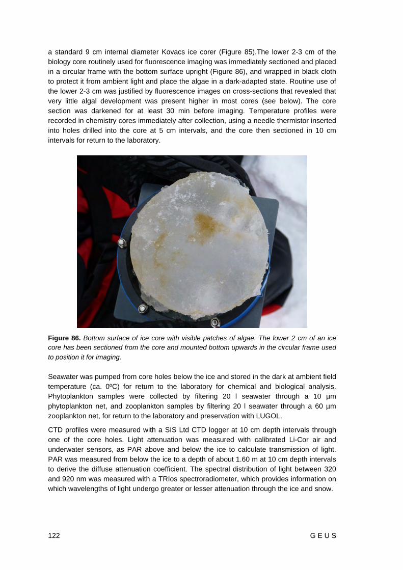
122 G E U S

a standard 9 cm internal diameter Kovacs ice corer (Figure 85).The lower 2-3 cm of the biology core routinely used for fluorescence imaging was immediately sectioned and placed in a circular frame with the bottom surface upright (Figure 86), and wrapped in black cloth to protect it from ambient light and place the algae in a dark-adapted state. Routine use of the lower 2-3 cm was justified by fluorescence images on cross-sections that revealed that very little algal development was present higher in most cores (see below). The core section was darkened for at least 30 min before imaging. Temperature profiles were recorded in chemistry cores immediately after collection, using a needle thermistor inserted into holes drilled into the core at 5 cm intervals, and the core then sectioned in 10 cm intervals for return to the laboratory.

Figure 86. Bottom surface of ice core with visible patches of algae. The lower 2 cm of an ice core has been sectioned from the core and mounted bottom upwards in the circular frame used

to position it for imaging. Seawater was pumped from core holes below the ice and stored in the dark at ambient field temperature (ca. 0ºC) for return to the laboratory for chemical and biological analysis. Phytoplankton samples were collected by filtering 20 l seawater through a 10 µm phytoplankton net, and zooplankton samples by filtering 20 l seawater through a 60 µm zooplankton net, for return to the laboratory and preservation with LUGOL.

CTD profiles were measured with a SIS Ltd CTD logger at 10 cm depth intervals through one of the core holes. Light attenuation was measured with calibrated Li-Cor air and underwater sensors, as PAR above and below the ice to calculate transmission of light. PAR was measured from below the ice to a depth of about 1.60 m at 10 cm depth intervals to derive the diffuse attenuation coefficient. The spectral distribution of light between 320 and 920 nm was measured with a TRIos spectroradiometer, which provides information on which wavelengths of light undergo greater or lesser attenuation through the ice and snow.

G E U S 123

14.3.2 Fluorescence Imaging

Fluorescence imaging of sea ice was performed in the field, to ensure minimum time between collection and imaging of algae. The instrument used for imaging is a Walz Imaging PAM (Pulse Amplitude Modulated) fluorometer (Walz Mess- und Regeltechnik, Germany) fitted with a lens imaging an area of 30 x 23 mm (Figure 87). Figure 87 also shows how we mounted the instrument in a light-proof box with an adjustable stage, allowing easy focusing of the image and maintaining the sample dark-adapted throughout measurements. Details of the principles and operation of the Imaging-PAM fluorometer are available in Hawes et al. (2012); briefly, we use the saturation pulse method to determine the two-dimensional distribution and activity of algal pigments in the ice, measuring the minimum (F0) and maximum (Fm) fluorescence of dark-adapted samples to a pulsed blue light. Measurements were performed at various settings of instrument light intensity and gain, depending on the amount of algae present in samples, and to ensure comparability of F0 and Fm between images, we calibrated and corrected their response to different instrument settings using both the manufacturer’s fluorescence standard and control sea ice with no algae. From images we also determined the maximal photochemical yield, (Fm - F0)/Fm or Fv/Fm, which provides an index, ranging from 0 to 1, that represents the ‘condition’ of the algal photosynthetic machinery. Maximal values of ca. 0.8 indicate ‘healthy’ active photosynthetic metabolism, with lower dark-adapted Fv/Fm observed when the photosynthetic condition becomes limited or stressed by unfavourable conditions. As Fv/Fm proved to be very low in most samples (see below), we did not use the imaging PAM to perform any light response curves for the ice algae. We made images of both the surface of the ice, and of cross-sections through the bottom 2 - 3 cm. After measurements, the imaged ice sample was returned to the dark at 0ºC for transport to the ship within 30 min.

14.3.3 On-board Laboratory Analyses

The 10-cm sections of the physico-chemistry core were weighed, thawed overnight at room temperature, and salinity and conductivity (temperature-corrected) measured. Water from the bottom 0-10 cm section was then filtered (0.22 µm) and frozen for nutrient analysis, and a 300 mL sub-sample filtered for analysis of spectral absorption properties of the ice (i.e. the extent to which material in the ice absorbs different wavelengths of light). The filtrate from this sample was then stored at 4ºC for analysis of CDOM (chromophoric dissolved organic matter). On some occasions the bottom slice was thawed in air-tight sealed containers for dissolved inorganic carbon (DIC) analysis. DIC sampling involved taking 2 mL of thawed ice and injecting it into glass tubes containing 0.4 ml 1N HCl for later analysis by infrared gas analysis. The imaged ice section from the biology core was thawed overnight at 0ºC in 0.22 µm-filtered seawater (50:50 v:v) to avoid osmotic shock before Phyto-PAM analysis, and a sub-sample taken and fixed with LUGOL for algal species identification. 300 ml of this thawed ice was filtered (GF/F) for chlorophyll analysis. The seawater from immediately under the ice was processed identically for the same analyses on the day of collection, except that 4 l was used for chlorophyll. On some days, additional filters were made for later analysis of algal pigments (by HPLC), PN:PP (particulate nitrogen : particulate phosphorus), and PN:PC (particulate nitrogen : particulate carbon).

124 G E U S

Figure 87. Fluorescence imaging set-up (left) with the Imaging-PAM Fluorometer. The principle of the method is that algae emit (fluoresce) red light into the camera when irradiated with blue light from the light source. Images were taken of the bottom surface of the ice, as shown in this diagram, or of cross-sections through the ice core section. The apparatus is enclosed in a light-proof box (right) to protect the core section from sunlight and ensure low light intensities relevant for sea ice throughout measurements.

All these analyses (nutrients, spectral absorption, CDOM, DIC, species identification and chlorophyll) will be completed in Denmark after de-mobilisation. They are all parameters that either affect the growth conditions of algae or describe the algal community, and will be important for providing a full explanation of the physiological studies carried out during the cruise. The ice core length, weight, temperature and conductivity data allow us to calculate porosity and brine volumes in the ice, so that concentrations can be expressed per unit brine volume and per unit area of sea ice.

Variable chlorophyll fluorescence of the thawed sample was measured using a Walz Phyto-PAM instrument. Three subsamples of the thawed ice were assayed in the cuvette of the Phyto-PAM instrument, taking care to maintain samples in darkness or very dim light. Dark-adapted minimum fluorescence yield (Fo) was first determined, followed by a measure of maximum fluorescence yield (Fm) during the application of a 0.6 s saturating irradiance pulse. Care was taken to ensure that the saturating pulse was the minimum required to obtain Fm. Fv /Fm was determined as with the imaging-PAM. In addition, rapid light curves (see Ralph and Gademan, 2005) were made for each sample.

14.4 Ice Conditions, Irradiance and Fluorescence Imaging The ice thickness varied from 1.07 m to 3.00 m amongst the stations sampled, with no trends in ice thickness along the transect of the cruise (Table 20). Snow thickness ranged from 5 to 15 cm, and temperatures at the bottom of the ice varied from -1.9ºC to -2.6ºC. A few cores had visible signs of recent ice growth, with very even, crystalline bases, but most cores had apparently older lower surfaces which had been stable or even thawing prior to collection. Almost all cores were annual sea ice rather than multi-year ice, and Figure 88

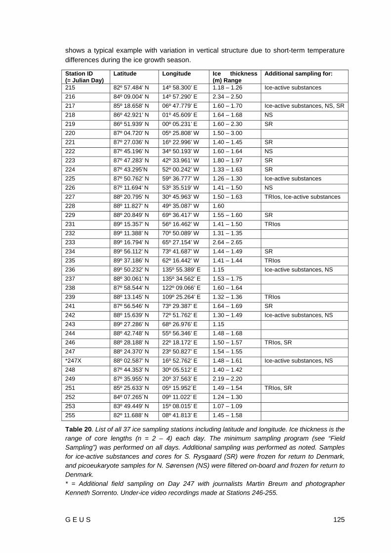
G E U S 125

shows a typical example with variation in vertical structure due to short-term temperature differences during the ice growth season.

Station ID (= Julian Day)

Latitude Longitude Ice thickness (m) Range

Additional sampling for:

215 82º 57.484’ N 14º 58.300’ E 1.18 – 1.26 Ice-active substances 216 84º 09.004’ N 14º 57.290’ E 2.34 – 2.50 217 85º 18.658’ N 06º 47.779’ E 1.60 – 1.70 Ice-active substances, NS, SR 218 86º 42.921’ N 01º 45.609’ E 1.64 – 1.68 NS 219 86º 51.939’ N 00º 05.231’ E 1.60 – 2.30 SR 220 87º 04.720’ N 05º 25.808’ W 1.50 – 3.00 221 87º 27.036’ N 16º 22.996’ W 1.40 – 1.45 SR 222 87º 45.196’ N 34º 50.193’ W 1.60 – 1.64 NS 223 87º 47.283’ N 42º 33.961’ W 1.80 – 1.97 SR 224 87º 43.295’N 52º 00.242’ W 1.33 – 1.63 SR 225 87º 50.762’ N 59º 36.777’ W 1.26 – 1.30 Ice-active substances 226 87º 11.694’ N 53º 35.519’ W 1.41 – 1.50 NS 227 88º 20.795’ N 30º 45.963’ W 1.50 – 1.63 TRIos, Ice-active substances 228 88º 11.827’ N 49º 35.087’ W 1.60 229 88º 20.849’ N 69º 36.417’ W 1.55 – 1.60 SR 231 89º 15.357’ N 56º 16.462’ W 1.41 – 1.50 TRIos 232 89º 11.388’ N 70º 50.089’ W 1.31 – 1.35 233 89º 16.794’ N 65º 27.154’ W 2.64 – 2.65 234 89º 56.112’ N 73º 41.687’ W 1.44 – 1.49 SR 235 89º 37.186’ N 62º 16.442’ W 1.41 – 1.44 TRIos 236 89º 50.232’ N 135º 55.389’ E 1.15 Ice-active substances, NS 237 88º 30.061’ N 135º 34.562’ E 1.53 – 1.75 238 87º 58.544’ N 122º 09.066’ E 1.60 – 1.64 239 88º 13.145’ N 109º 25.264’ E 1.32 – 1.36 TRIos 241 87º 56.546’ N 73º 29.387’ E 1.64 – 1.69 SR 242 88º 15.639’ N 72º 51.762’ E 1.30 – 1.49 Ice-active substances, NS 243 89º 27.286’ N 68º 26.976’ E 1.15 244 88º 42.748’ N 55º 56.346’ E 1.48 – 1.68 246 88º 28.188’ N 22º 18.172’ E 1.50 – 1.57 TRIos, SR 247 88º 24.370’ N 23º 50.827’ E 1.54 – 1.55 *247X 88º 02.587’ N 16º 52.762’ E 1.48 – 1.61 Ice-active substances, NS 248 87º 44.353’ N 30º 05.512’ E 1.40 – 1.42 249 87º 35.955’ N 20º 37.563’ E 2.19 – 2.20 251 85º 25.633’ N 05º 15.952´E 1.49 – 1.54 TRIos, SR 252 84º 07.265´N 09º 11.022’ E 1.24 – 1.30 253 83º 49.449’ N 15º 08.015’ E 1.07 – 1.09 255 82º 11.688’ N 08º 41.813’ E 1.45 – 1.58

Table 20. List of all 37 ice sampling stations including latitude and longitude. Ice thickness is the range of core lengths (n = 2 – 4) each day. The minimum sampling program (see “Field Sampling”) was performed on all days. Additional sampling was performed as noted. Samples for ice-active substances and cores for S. Rysgaard (SR) were frozen for return to Denmark, and picoeukaryote samples for N. Sørensen (NS) were filtered on-board and frozen for return to Denmark. * = Additional field sampling on Day 247 with journalists Martin Breum and photographer Kenneth Sorrento. Under-ice video recordings made at Stations 246-255.

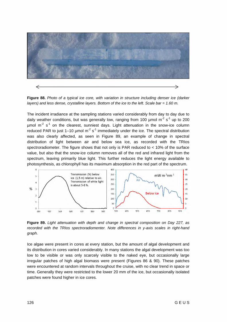
126 G E U S

Figure 88. Photo of a typical ice core, with variation in structure including denser ice (darker layers) and less dense, crystalline layers. Bottom of the ice to the left. Scale bar = 1.60 m.

The incident irradiance at the sampling stations varied considerably from day to day due to daily weather conditions, but was generally low, ranging from 100 µmol m-2 s-1 up to 200 µmol m-2 s-1 on the clearest, sunniest days. Light attenuation in the snow-ice column reduced PAR to just 1–10 µmol m-2 s-1 immediately under the ice. The spectral distribution was also clearly affected, as seen in Figure 89, an example of change in spectral distribution of light between air and below sea ice, as recorded with the TRIos spectroradiometer. The figure shows that not only is PAR reduced to < 10% of the surface value, but also that the snow-ice column removes all of the red and infrared light from the spectrum, leaving primarily blue light. This further reduces the light energy available to photosynthesis, as chlorophyll has its maximum absorption in the red part of the spectrum.

Figure 89. Light attenuation with depth and change in spectral composition on Day 227, as recorded with the TRIos spectroradiomenter. Note differences in y-axis scales in right-hand graph. Ice algae were present in cores at every station, but the amount of algal development and its distribution in cores varied considerably. In many stations the algal development was too low to be visible or was only scarcely visible to the naked eye, but occasionally large irregular patches of high algal biomass were present (Figures 86 & 90). These patches were encountered at random intervals throughout the cruise, with no clear trend in space or time. Generally they were restricted to the lower 20 mm of the ice, but occasionally isolated patches were found higher in ice cores.

G E U S 127

Spatial variations in algal biomass and Fv /Fm within these patches were easy to document with fluorescence imaging. Figure 90 shows both surface and cross-sections of a typical visible patch, showing the high biomass but limited penetration of algae up into the core. Fv /Fm was very low in most patches (< 0.1), but rose to 0.2 – 0.4 when measured in the Phyto-PAM after thawing of the core slice; this was still considerably lower than Fv /Fm in seawater phytoplankton (Fv /Fm > 0.5).

Figure 90. Examples of images of F0 (minimum variable fluorescence) obtained in the field with the Imaging-PAM fluorometer, from ice cores with high biomass patches. Colour scales from red (low biomass) to blue (high biomass), but is not comparable between images due to different instrument settings. Left: Surface view of bottom of an ice core with a high biomass patch. Middle: Cross-section through a patch, showing algal development limited to the lower 15 - 20 mm of the ice. Right: Cross-section of a patch isolated ca. 5 – 7 cm from the bottom of a core, in which the lower 5 cm lacking algae appeared to be recent ice growth. Circles are AOIs (‘Areas of Interest’) used to quantify aspects of algal photobiology at specific areas of the image. All pictures 30 x 23 mm. Unlike the large visible patches, the ‘background’ algal community, almost invisible to the naked eye but usually distributed very evenly across the width of cores, showed a strong trend during the cruise. Biomass was initially high during transit across the Gakkel Ridge and into the south-western corner of the Amundsen Basin, fell to low levels over the western Lomonosov Ridge and past the North Pole, and then rose dramatically again in the eastern Lomonosov Ridge stations. The distribution of this type of algal development is shown in Figure 91, in which the algal material is visible in its brine channels, amongst the non-fluorescing ice crystal structure, and again is primarily restricted to the lower 10 – 15 mm of the ice core. Although high sensitivity settings were required in fluorescence imaging to detect algae in the stations with lowest biomass, the method successfully resolved both the spatial and vertical distribution of these populations at all stations.

128 G E U S

Figure 91. Examples of images of F0 (minimum variable fluorescence) obtained in the field with the Imaging-PAM fluorometer in cores without large visible patches. Colour scales from red (low biomass) to blue (high biomass). (Left) Surface view of a core showing extensive algal development throughout. Circles are AOIs (‘Areas of Interest’) used to quantify aspects of algal photobiology at specific areas of the image. (Right) Cross-section of the bottom of a core, with the depth of algal development identified in rectangular box. All pictures 30 x 23 mm.

14.5 Perspectives and Future Outlook Although a full understanding of the patterns in algal distribution and photobiology awaits analysis of samples being returned to Denmark, some preliminary conclusions from the fluorescence imaging and other on-board work are possible. Our data suggest that the late summer-early autumn ice algae in the region of the Arctic Ocean covered by LOMROG III are patchy in distribution, often present in low amounts but almost always with measurable biomass and activity. The fluorescence data, especially when imaged in intact ice, suggest that algal photosynthetic metabolism had been subject to considerable resource limitation and stress prior to the cruise, and the limited recovery of Fv /Fm in thawed ice suggests this stress has been chronic. Lavoie et al. (2005), in modelling Arctic Ocean ice algal biomass, have suggested that ice algal growth is light-limited early in the season, and becomes nutrient-limited later in the season. Nutrient limitation is certainly a prime candidate to explain our results, and this will be determined by our nutrient analyses. However, light intensities are very low in situ, and our photosynthesis data suggest that the algae are probably light-limited also, with light and nutrient co-limitation occurring at most sampling stations.

14.6 Acknowledgements We thank the crew of Oden for their hospitality, help and patience throughout the cruise, and the support staff who made sampling possible, especially our helicopter pilots and meteorologists. We also thank all LOMROG III participants for useful discussions and

G E U S 129

constructive feedback that improved our understanding of the Arctic system, and express our particular gratitude to Chief Scientist Christian Marcussen for providing the unparalleled ice sampling opportunities on LOMROG III. The authors’ research on sea ice algal photobiology is supported by grants from the Carlsberg Foundation and Brødrene Hartmann’s Fund.

14.7 References Gradinger, R. 2009: Sea-ice algae: major contributors to primary production and algal

biomass in the Chukchi and Beaufort Seas during May/June 2002. Deep Sea Research 56,1201–1212.

Gosselin, M., Levasseur, M., Wheeler, P.A., Horner, R.A. & Booth, B.C. 1997: New measurements of phytoplankton and ice algal production in the Arctic Ocean. Deep-Sea Research II, 44, 1623-1644.

Hawes, I., Lund-Hansen, L.C., Sorrell, B.K., Nielsen, M.H., Borzák, R. & Buss, I. 2012: Photobiology of sea ice algae during initial spring growth in Kangerlussuaq, West Greenland: insights from imaging variable chlorophyll fluorescence of ice cores. Photosynthesis Research, doi: 10.1007/s11120-012-9736-7.

Krembs, C., Eicken, H. & Deming, J.W. 2011: Exopolymer alteration of physical properties of sea ice and implications for ice habitability and biogeochemistry in a warmer Arctic. Proceedings of the National Academy of Sciences 108, 3653–3658.

Lavoie, D., Denman, K. & Michel, C. 2005: Modeling ice algal growth and decline in a seasonally ice-covered region of the Arctic (Resolute Passage, Canadian Archipelago). Journal of Geophysical Research 110, C11009, doi:10.1029/2005JC002922.

Ralph, P.J. & Gademan, R. 2005: Rapid light curves: A powerful tool to assess photosynthetic activity. Aquatic Botany 82, 222–237.

130 G E U S


G E U S 131

15. Characterization of Bioactive Gram-positive Spore-forming Arctic Bacteria

By Nikolaj Grønnegaard Vynne, National Food Institute (DTU Food)

15.1 Introduction There is currently an increasing awareness of the need for novel antibiotics to combat emerging multiresistant pathogens, and natural products of bacterial origins have a long history of contributing biologically active compounds for the clinical pipeline. The actinobacteria are considered one of the most prolific sources of biologically active natural compounds (Bull & Stach, 2007), and recent studies have confirmed the existence of actinobacterial species which require seawater for growth (Jensen et al., 2007). Very few studies of Arctic actinobacteria exist; however based on our experience from the LOMROG II expedition we believe such bacteria might represent an untapped source of novel bioactive compounds. In order to investigate this, samples were collected in the high Arctic to establish bioactive potential among Arctic Gram-positive spore forming marine bacteria, specifically aimed at detection of novel bacterial diversity and accompanying novel antagonistic chemical compounds.

15.2 Aim The aim of this project was to collect samples from hitherto under-explored areas in the Arctic Ocean, with a focus on obtaining novel Gram-positive spore forming bacteria, specifically actinobacteria. The bioactive potential of these bacteria will be investigated, with a focus on antibiosis. The physiology of selected strains of interest will be studied in detail with the aim to understand how different nutrient sources impact secondary metabolism, e.g. by growth on ‘natural’ substrates such as chitin. Work to increase the culturability of bacteria from Arctic environmental samples may also be included.

15.3 Scientific Work on Board On board icebreaker Oden, samples were collected from sediment, dredged mud, ice cores and the water column (Table 21). Sediment samples were obtained from piston coring from a depth of 5-7 m below the sea floor (Figure 92). The piston coring was performed by a team from Stockholm University led by Richard Gyllencreutz.

Mud samples were obtained from rocks retrieved during dredging. These samples were impossible to handle aseptically, and thus are not suited for ecology-related studies.

132 G E U S

Figure 92. The 'Core catcher' of the piston corer from which surplus sediment is sampled for microbial analyses (Photo: Ragner Jerre).

Seawater samples were obtained from CTD stations. Ship-based CTD stations used a rosette equipped with 24 7 l Niskin bottles, and water was sampled for this project at 10 m, 300 m and the bottom (ca. 20 m above the sea floor). Helicopter CTD stations provided water samples from 10 m and 200 m. All CTD work was performed by Steffen Olsen and Rasmus Tonboe of DMI. Kajsa Tönneson performed water sampling on helicopter stations.

Ice core samples were retrieved using a Kovacs ice corer (Figure 93). The bottom 2 cm of each ice core was placed in an ethanol washed plastic bag and stored at -20ºC. Figure 93. Nikolaj Vynne (left) and Gorm Dybkjær on the Arctic ice, preparing to drill an ice core (Photo: Markus Karasti).

G E U S 133

In total 120 environmental samples were obtained (Table 21), with an additional 23 samples obtained from the Microbial Communities project led by Pauline Snoeijs (see Table 10 in Chapter 12. No sample was obtained from station 1). The samples were processed for safe storage until detailed analyses in a bacteriological laboratory are possible. Two strategies for storage were pursued in order to allow for retrieval of as much culturable bacterial diversity as possible. Samples were split in two fractions, and glycerol was added to 17% for one fraction to allow storage at -80ºC which is a routine storage protocol for bacterial cultures. The rest of the sample was held at 4ºC to allow for investigation of the fraction of bacteria which may not respond well to storage at -80ºC, e.g. due to crystalline formations in the cell membrane during the freezing process. Ice core samples were stored at -20ºC with no processing.

Long-term incubations at low temperature (10ºC) were initiated aboard Oden using two growth substrates. Both substrates were oligotrophic; one consisted of seawater supplemented with agar, the other of seawater with 100 mg l-1 peptone and 500 mg l-1 mannitol. Both substrates were supplemented with 5 µg ml-1 rifampicin and an antifungal agent. The low temperature incubations will be continued for a minimum of 3 months. All sediment and mud samples were inoculated on plates (Figure 93), as was a subset of CTD water samples.

Figure 93. Arctic sediment samples inoculated on nutrient poor growth substrate.

134 G E U S

Table 1. Environmental samples obtained during LOMROG III for studies of bioactive Gram-positive spore forming bacteria. Sample ID

Date

Latitude dd:mm.mm

Longitude dd:mm.mm

Bacterial project station

Source

L3-1 02-08-2012 82:57.48 N 14:55.98 E Ship CTD 1 CTD 10 m

L3-2 02-08-2012 82:57.48 N 14:55.98 E Ship CTD 1 CTD 300 m

L3-3 02-08-2012 82:57.48 N 14:55.98 E Ship CTD 1 CTD 2625 m

L3-4 03-08-2012 84:32.14 N 13:20.25 E Ice CTD 1 CTD 10 m

L3-5 04-08-2012 85:33.07 N 6:27.48 E Ice CTD 2 CTD 10 m

L3-6 05-08-2012 86:44.59 N 1:57.31 E Ship CTD 2 CTD 10 m

L3-7 05-08-2012 86:44.59 N 1:57.31 E Ship CTD 2 CTD 300 m

L3-8 05-08-2012 86:44.59 N 1:57.31 E Ship CTD 2 CTD 4248 m

L3-9 06-08-2012 87:02.38 N 3:27.35 W Ice CTD 3 CTD 10 m

L3-10 07-08-2012 87:06 N 6:46 W Ice station 1 Ice, top (10 cm)

L3-11 07-08-2012 87:06 N 6:46 W Ice station 1 Ice, middle (80 cm)

L3-12 07-08-2012 87:06 N 6:46 W Ice station 1 Ice, bottom (180 cm)

L3-13 07-08-2012 87:06 N 6:46 W Ice station 1 Melt water pond

L3-14 07-08-2012 87:06 N 6:46 W Ice station 1 Ice core, at 150 cm

L3-15 07-08-2012 87:19.50 N 13:27.90 W Ice CTD 4 CTD 10 m

L3-16 08-08-2012 87:39 N 23:40 W Ice station 2 Ice core, bottom 10 cm of 300 cm

L3-17 09-08-2012 87:46 N 37:39 W Ice station 3 Ice core, bottom 2 cm of 145 cm

L3-18 09-08-2012 87:46.20 N 37:45.45 W Ship CTD 3 CTD 10 m

L3-19 09-08-2012 87:46.21 N 37:45.45 W Ship CTD 3 CTD 300 m

L3-20 09-08-2012 87:46.22 N 37:45.45 W Ship CTD 3 CTD 3500 m

L3-21 10-08-2012 87:79.69 N 43:02.74 W Coring 1 Sediment coring, top 10 cm of 0,5 m core

L3-22 10-08-2012 87:46 N 52:53 W Ice station 4 Ice core, at 330 cm of 345 cm ice

L3-23 10-08-2012 87:39.47 N 58:53.27 W Ice CTD 6 CTD 10 m

L3-24 11-08-2012 87:72.44 N 44:51.44 W Coring 2 Sediment coring, bottom 10 cm of 4 m core

L3-25 11-08-2012 87:45.14 N 54:41.54 W Zooplankton Sea water

L3-26 11-08-2012 87:39.47 N 58:53.27 W Ice CTD 7 CTD 10 m

L3-27 12-08-2012 87:49.28 N 59:38.20 W Coring 3-1 Sediment coring, top 10 cm. Failed core.

L3-28 12-08-2012 87:49.28 N 59:38.20 W Coring 3-2 Sediment coring, bottom of 7 m core

L3-29 08-08-2012 87:44.27 N 26:58.48 W Ice CTD 5 CTD 10 m

L3-30 12-08-2012 87:49 N 63:28 W Ice station 5 Ice core, bottom 2 cm of 345 cm core

L3-31 12-08-2012 87:38.35 N 68:55.88 W Ice CTD 8 CTD 10 m

L3-32 13-08-2012 88:15.93 N 43:10.52 W Ice CTD 9 CTD 10 m

L3-33 15-08-2012 88:12 N 46:03 W Ice station 6 Ice core, bottom 2 cm of 150 cm core

L3-34 15-08-2012 88:15.04 N 46:23.50 W Coring 4 Sediment from core catcher, 6,5 m core

L3-35 14-08-2012 88:14.09 N 29:57.05 W Ice CTD 10 CTD 10 m

L3-36 15-08-2012 88:16.32 N 58:01.00 W Ice CTD 11 CTD 10 m

L3-37 15-08-2012 88:11.52 N 55:41.04 W Coring 5 Sediment from core catcher, 6,8 m core

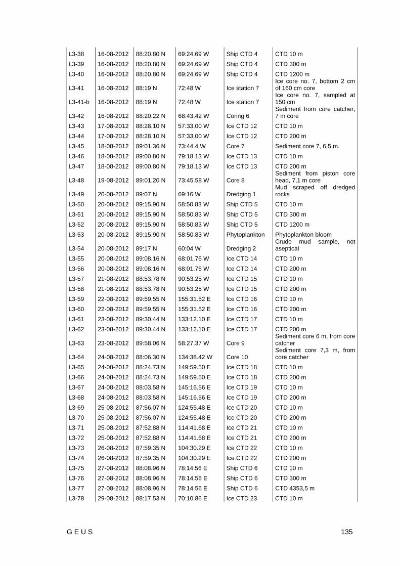
G E U S 135

L3-38 16-08-2012 88:20.80 N 69:24.69 W Ship CTD 4 CTD 10 m

L3-39 16-08-2012 88:20.80 N 69:24.69 W Ship CTD 4 CTD 300 m

L3-40 16-08-2012 88:20.80 N 69:24.69 W Ship CTD 4 CTD 1200 m

L3-41 16-08-2012 88:19 N 72:48 W Ice station 7 Ice core no. 7, bottom 2 cm of 160 cm core

L3-41-b 16-08-2012 88:19 N 72:48 W Ice station 7 Ice core no. 7, sampled at 150 cm

L3-42 16-08-2012 88:20.22 N 68:43.42 W Coring 6 Sediment from core catcher, 7 m core

L3-43 17-08-2012 88:28.10 N 57:33.00 W Ice CTD 12 CTD 10 m

L3-44 17-08-2012 88:28.10 N 57:33.00 W Ice CTD 12 CTD 200 m

L3-45 18-08-2012 89:01.36 N 73:44.4 W Core 7 Sediment core 7, 6,5 m.

L3-46 18-08-2012 89:00.80 N 79:18.13 W Ice CTD 13 CTD 10 m

L3-47 18-08-2012 89:00.80 N 79:18.13 W Ice CTD 13 CTD 200 m

L3-48 19-08-2012 89:01.20 N 73:45.58 W Core 8 Sediment from piston core head, 7,1 m core

L3-49 20-08-2012 89:07 N 69:16 W Dredging 1 Mud scraped off dredged rocks

L3-50 20-08-2012 89:15.90 N 58:50.83 W Ship CTD 5 CTD 10 m

L3-51 20-08-2012 89:15.90 N 58:50.83 W Ship CTD 5 CTD 300 m

L3-52 20-08-2012 89:15.90 N 58:50.83 W Ship CTD 5 CTD 1200 m

L3-53 20-08-2012 89:15.90 N 58:50.83 W Phytoplankton Phytoplankton bloom

L3-54 20-08-2012 89:17 N 60:04 W Dredging 2 Crude mud sample, not aseptical

L3-55 20-08-2012 89:08.16 N 68:01.76 W Ice CTD 14 CTD 10 m

L3-56 20-08-2012 89:08.16 N 68:01.76 W Ice CTD 14 CTD 200 m

L3-57 21-08-2012 88:53.78 N 90:53.25 W Ice CTD 15 CTD 10 m

L3-58 21-08-2012 88:53.78 N 90:53.25 W Ice CTD 15 CTD 200 m

L3-59 22-08-2012 89:59.55 N 155:31.52 E Ice CTD 16 CTD 10 m

L3-60 22-08-2012 89:59.55 N 155:31.52 E Ice CTD 16 CTD 200 m

L3-61 23-08-2012 89:30.44 N 133:12.10 E Ice CTD 17 CTD 10 m

L3-62 23-08-2012 89:30.44 N 133:12.10 E Ice CTD 17 CTD 200 m

L3-63 23-08-2012 89:58.06 N 58:27.37 W Core 9 Sediment core 6 m, from core catcher

L3-64 24-08-2012 88:06.30 N 134:38.42 W Core 10 Sediment core 7,3 m, from core catcher

L3-65 24-08-2012 88:24.73 N 149:59.50 E Ice CTD 18 CTD 10 m

L3-66 24-08-2012 88:24.73 N 149:59.50 E Ice CTD 18 CTD 200 m

L3-67 24-08-2012 88:03.58 N 145:16.56 E Ice CTD 19 CTD 10 m

L3-68 24-08-2012 88:03.58 N 145:16.56 E Ice CTD 19 CTD 200 m

L3-69 25-08-2012 87:56.07 N 124:55.48 E Ice CTD 20 CTD 10 m

L3-70 25-08-2012 87:56.07 N 124:55.48 E Ice CTD 20 CTD 200 m

L3-71 25-08-2012 87:52.88 N 114:41.68 E Ice CTD 21 CTD 10 m

L3-72 25-08-2012 87:52.88 N 114:41.68 E Ice CTD 21 CTD 200 m

L3-73 26-08-2012 87:59.35 N 104:30.29 E Ice CTD 22 CTD 10 m

L3-74 26-08-2012 87:59.35 N 104:30.29 E Ice CTD 22 CTD 200 m

L3-75 27-08-2012 88:08.96 N 78:14.56 E Ship CTD 6 CTD 10 m

L3-76 27-08-2012 88:08.96 N 78:14.56 E Ship CTD 6 CTD 300 m

L3-77 27-08-2012 88:08.96 N 78:14.56 E Ship CTD 6 CTD 4353,5 m

L3-78 29-08-2012 88:17.53 N 70:10.86 E Ice CTD 23 CTD 10 m

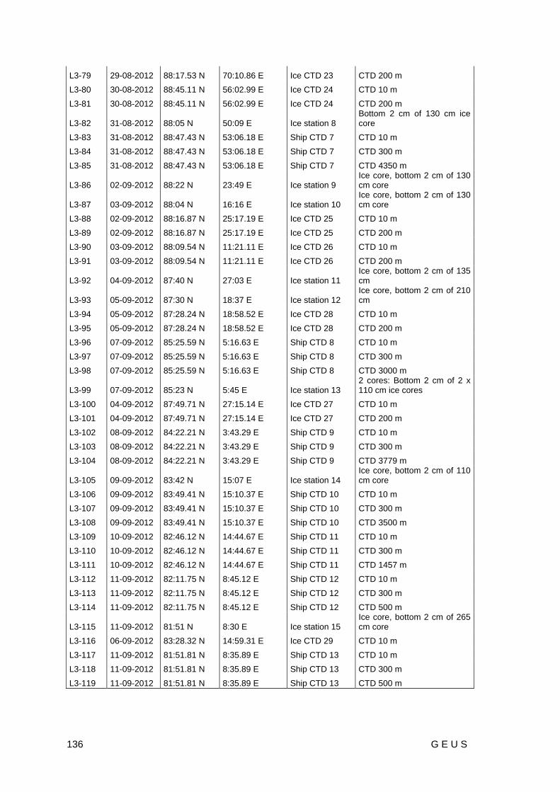
136 G E U S

L3-79 29-08-2012 88:17.53 N 70:10.86 E Ice CTD 23 CTD 200 m

L3-80 30-08-2012 88:45.11 N 56:02.99 E Ice CTD 24 CTD 10 m

L3-81 30-08-2012 88:45.11 N 56:02.99 E Ice CTD 24 CTD 200 m

L3-82 31-08-2012 88:05 N 50:09 E Ice station 8 Bottom 2 cm of 130 cm ice core

L3-83 31-08-2012 88:47.43 N 53:06.18 E Ship CTD 7 CTD 10 m

L3-84 31-08-2012 88:47.43 N 53:06.18 E Ship CTD 7 CTD 300 m

L3-85 31-08-2012 88:47.43 N 53:06.18 E Ship CTD 7 CTD 4350 m

L3-86 02-09-2012 88:22 N 23:49 E Ice station 9 Ice core, bottom 2 cm of 130 cm core


L3-88 02-09-2012 88:16.87 N 25:17.19 E Ice CTD 25 CTD 10 m

L3-89 02-09-2012 88:16.87 N 25:17.19 E Ice CTD 25 CTD 200 m

L3-90 03-09-2012 88:09.54 N 11:21.11 E Ice CTD 26 CTD 10 m

L3-91 03-09-2012 88:09.54 N 11:21.11 E Ice CTD 26 CTD 200 m

L3-92 04-09-2012 87:40 N 27:03 E Ice station 11 Ice core, bottom 2 cm of 135 cm

L3-93 05-09-2012 87:30 N 18:37 E Ice station 12 Ice core, bottom 2 cm of 210 cm

L3-94 05-09-2012 87:28.24 N 18:58.52 E Ice CTD 28 CTD 10 m

L3-95 05-09-2012 87:28.24 N 18:58.52 E Ice CTD 28 CTD 200 m

L3-96 07-09-2012 85:25.59 N 5:16.63 E Ship CTD 8 CTD 10 m

L3-97 07-09-2012 85:25.59 N 5:16.63 E Ship CTD 8 CTD 300 m

L3-98 07-09-2012 85:25.59 N 5:16.63 E Ship CTD 8 CTD 3000 m

L3-99 07-09-2012 85:23 N 5:45 E Ice station 13 2 cores: Bottom 2 cm of 2 x 110 cm ice cores

L3-100 04-09-2012 87:49.71 N 27:15.14 E Ice CTD 27 CTD 10 m

L3-101 04-09-2012 87:49.71 N 27:15.14 E Ice CTD 27 CTD 200 m

L3-102 08-09-2012 84:22.21 N 3:43.29 E Ship CTD 9 CTD 10 m

L3-103 08-09-2012 84:22.21 N 3:43.29 E Ship CTD 9 CTD 300 m

L3-104 08-09-2012 84:22.21 N 3:43.29 E Ship CTD 9 CTD 3779 m


L3-106 09-09-2012 83:49.41 N 15:10.37 E Ship CTD 10 CTD 10 m

L3-107 09-09-2012 83:49.41 N 15:10.37 E Ship CTD 10 CTD 300 m

L3-108 09-09-2012 83:49.41 N 15:10.37 E Ship CTD 10 CTD 3500 m

L3-109 10-09-2012 82:46.12 N 14:44.67 E Ship CTD 11 CTD 10 m

L3-110 10-09-2012 82:46.12 N 14:44.67 E Ship CTD 11 CTD 300 m

L3-111 10-09-2012 82:46.12 N 14:44.67 E Ship CTD 11 CTD 1457 m

L3-112 11-09-2012 82:11.75 N 8:45.12 E Ship CTD 12 CTD 10 m

L3-113 11-09-2012 82:11.75 N 8:45.12 E Ship CTD 12 CTD 300 m

L3-114 11-09-2012 82:11.75 N 8:45.12 E Ship CTD 12 CTD 500 m


L3-116 06-09-2012 83:28.32 N 14:59.31 E Ice CTD 29 CTD 10 m

L3-117 11-09-2012 81:51.81 N 8:35.89 E Ship CTD 13 CTD 10 m

L3-118 11-09-2012 81:51.81 N 8:35.89 E Ship CTD 13 CTD 300 m

L3-119 11-09-2012 81:51.81 N 8:35.89 E Ship CTD 13 CTD 500 m

G E U S 137

15.4 Work at the National Food Institute, DTU (Denmark)

15.4.1 Culturing and Identification of Gram-positive Spore Forming Bacteria

Culturable counts on standard growth substrate (Marine Agar 2216) will be determined. A range of alternative substrates will be used to selectively isolate Gram-positive spore forming bacteria. The isolated actinobacteria will be identified by 16S rRNA gene sequence, phenotypic tests and morphological features to allow comparison of actinobacterial diversity in the Arctic with that in previously studied areas such as tropical Pacific sediments (Jensen et al., 2005).

The ability to grow bacteria in pure cultures is an essential prerequisite for many methods within bacteriology; yet standard laboratory procedures only allow for growth of 0.1-1% of the bacterial cells found in environmental samples. Growth substrates based on energy sources found in the natural environment, such as chitin, will be tested for their influence to increase culturable counts or change the culturable fraction of environmental samples.

15.4.2 Screening of Bacterial Cultures for Bioactive Properties

All isolated bacterial strains will be screened for antagonism against multiple target strains, including Staphylococcus aureus and the fish pathogenic marine strain Vibrio anguillarum 90-11-287. Antivirulence activity will be detected by testing for influence on the agr signaling system in S. aureus. Other biological activities may also be pursued, for instance cytotoxic effects. In an effort to further understand the interactions within bacterial populations, the isolated strains may be included in mixed culture incubations to investigate the effect on production of antagonistic compounds.

15.4.3 Genome Sequencing of Bioactive Bacterial Strains

To investigate the genomic potential for production of bioactive compounds, some isolated strains will be whole genome sequenced. Through ‘genome mining’, this will allow an assessment of the potential for secondary metabolite production by the sequenced strains, and may provide clues on the type of compounds that are produced and under which growth conditions production takes place. Additionally, whole genome sequences are of great use if targeted cloning and expression of biosynthetic pathways in a heterologous host is pursued.

15.5 Results Most of the analyses of the obtained samples require working aseptically, which is not possible given the conditions on board Oden. Additionally, specialized equipment and hazardous chemicals are not appropriate for use in field work. Hence, further analyses of

138 G E U S

the collected samples will be carried out at the National Food Institute, DTU (Denmark). No results were available at the time of writing this report.

15.6 References Bull, A.T. & Stach, E. (2007): Marine actinobacteria: new opportunities for natural product

search and discovery. Trends in Microbiology 15, 491-499.

Jensen, P.R., Gontang, E., Mafnas, C., Mincer, T.J. & Fenical, W. (2005): Culturable marine actinomycete diversity from tropical Pacific Ocean sediments. Environmental Microbiology 7, 1039-1048.

Jensen, P.R., Williams, P.G., Dong-Chan, O., Zeigler, L. & Fenical, W. (2007): Species-specific secondary metabolite production in marine actinomycetes of the genus Salinispora. Applied and Environmental Microbiology 73, 1146-1152.

G E U S 139

16. Sea Ice Temperature

By Gorm Dybkjær & Rasmus Tonboe, Danish Meteorological Institute (DMI)

16.1 Introduction Temperatures of snow and ice are vital parameters for understanding the freezing and melting of sea ice. Measurements of these temperatures are not available through traditional observations, but only as proxy measurements from a scarcely distributed Arctic observation network that mainly consist of air temperature sensors on drifting buoys. Information of the snow and ice temperatures from satellite observations can provide important information about the vertical thermodynamics and thereby be essential for calculation of ice growth and melt and also assist in calibrating and validating the multilayer sea ice models in e.g. ocean and weather models.

Figure 95. Oden seen from helicopter. On Monkey Island above the Bridge, Infra-Red and Microwave instruments are placed to measure sea ice temperatures (red arrow).

However, it is not trivial to measure snow and ice temperatures from satellite because a number of conditions have to be accounted for. In order to obtain reliable snow and ice temperatures from space, it is necessary to account for different states of snow and ice, the presents of melt ponds and the fraction of open water inside the footprint of the satellite

140 G E U S

measurement. To quantify these contributions, detailed and simultaneous sampling of the parameters of interest can provide vital knowledge to understand this interaction.

The aim of the Sea Ice Temperature project participating in the LOMROG III cruise is to collect a large data set to investigate the influence and correlation between actual snow and ice temperatures, satellite measurements and the variables that influence these measurements. This will provide valuable knowledge for both thermodynamically modelling and algorithm development in remote sensing based applications.

The parameters that are measured simultaneously and that subsequently will be collocated are:

L-band microwave and thermal infrared brightness temperatures from identical satellite and ship borne instruments (Figure 95).

Photos of the ship borne L-band and TIR instrument footprints (Figure 101).

Synoptic ship data: air temperature, cloud height and wind speed (recorded by SMHI).

Continuous snow and ice temperature profiles from 8 mass balance buoys deployed between Greenland and the North Pole (Figure 97, 98 & 99).

In situ measurements of snow and ice characteristics recorded throughout the cruise (Figure 98): temperatures, salinity, density and snow characteristics.

The application of this collocated data set is to develop and improve sea ice temperature measurements from satellite. Daily distributed temperature fields from satellite instruments can improve the initial conditions of numerical ocean and atmosphere models, by adding large amount of valuable information to the sparsely distributed traditional observation network that Arctic ocean and atmosphere models rely on today. The project scientists have large experience in fieldwork and data sampling (Tonboe and Hansson, 2006; Dybkjær et al., 2011), modelling (Tonboe et al., 2011), monitoring and calibration/validation processes (Dybkjaer et al., 2012; Høyer et al., 2012).

Figure 96. Field work on the ice – a mass balance buoy has been deployed (left) and an ice core is being analysed (right). It takes patience to measure a temperature profile …

G E U S 141

16.2 Instruments and data

16.2.1 L-band, Thermal Infrared and Photos

On the top deck of Oden, on “Monkey Island”, we have deployed instruments that are identical to some operating satellite instruments that cover the Arctic Ocean on a daily basis (Figure 95). The instruments are thermal infrared and L-band microwave radiometers that measure the surface brightness temperatures. The calibrated infrared radiometer can be directly compared to a satellite based infrared sea ice temperature product that is running operational at DMI. The collocation of the satellite product with the identical ship borne instrument and in situ observations will provide valuable information for future development, calibration and validation of this product.

The microwave radiometer is identical to the instrument on board the SMOS satellite that originally is designed to measure soil moisture and ocean salinity. This instrument has also proven valuable for estimation of sea ice thickness of new ice (Kaleschke, 2006). This work is still at research level. The TIR and microwave instruments in combination provide information on both the skin temperature and of the internal snow and sea ice temperature and properties. The collocation of these data along with other measurements recorded during the LOMROG expedition will be subject to future research on, e.g. the potential of estimating fraction of open water in sea ice regions.

Along with these instruments we have also mounted an ordinary camera that continuously provides information of the fraction of water inside the field of view of the instruments. The

Figure 97. Sea ice mass balance buoy number 4 deployed on August 14, at position 88.35N 30.77W. The yellow box contains data logger, satellite communication and battery pack. The white stick holds the top of the thermistor string above the snow/ice surface, so that the temperature profile is measured from approximately 0.5m above the surface and down through the snow, ice and water.

142 G E U S

satellite and ship borne instruments will be matched up with ice/water fraction values calculated from the photos and the in situ measurements of snow and ice properties carried out from numerous helicopter sites during the cruise.

Figure 98. Positions of the 8 deployed mass balance buoys (coloured circles) and in situ sites (red crosses) until September 5.

16.2.2 Mass Balance Buoys

To investigate melting and freezing processes of sea ice in details we deployed 8 drifting buoys (Figure 97 & 98) which are constructed to measure the snow/ice temperature profile continuously. A temperature string attached to the buoys measure temperature at a 2 cm resolution from the air above, through the snow and ice and into the ocean water. Via an iridium telephone connection the buoys report bi-hourly on their position and temperature measurements.

16.2.3 Ship Data

Throughout LOMROG III, the Swedish Meteorological and Hydrological Institute (SMHI) has recorded synoptic data. Of special relevance for this project are cloud information, irradiation/radiation, air temperature (Figure 100), wind speed and direction and

G E U S 143

occasionally also sea surface temperature. These data will also be part of the collocated Sea Ice Temperature data set.

Figure 99. Twenty-one temperature profiles for buoy number 6. The large temperature variations on the left of the temperature profile are air temperatures and on the far right side of the figure, one sees the temperature of the ocean/ice interface.

16.2.4 In Situ Sampling

In situ sampling of snow and ice characteristics are done approximately every second day – at 23 sites. The in situ work consists of a snow description: grain size, layer description, density, salinity and temperature profile. The sea ice description consists of temperature and salinity profiles. In situ works is illustrated in Figure 96 & 102 shows salinity profiles from 14 ice core analyses. Parallel to this in situ work, Lars Chresten Lund-Hansen and Brian Sorrell from the ice algae project (Chapter14) perform frequent ice core analysis including density profiling. These data are kindly made available for the ice temperature project.

16.2.5 Satellite Data

Multiple daily Arctic coverage of satellite borne L-band and TIR data are received and stored at DMI, along with an operational TIR based Ice and Sea surface temperature product. These satellite data will be part of the collocated matchup data set that will be prepared after the expedition.

144 G E U S

Figure 100. Collocated air temperature measurements from ship (red curve), portable infra-red (green curve), ISAR - high precision infra-red (blue crosses) and L-band microwave polarisation (purple dots). The recording is from day 242.

16.3 Data Samples A few raw data samples from the sea ice temperature data sets are presented here. No post processing has been performed at this time.

Figure 101 [1-15]. A 15 minute photo sequence of the L-band and TIR radiometer footprint. The photos are recorded on day 242 between 12:00z and 12:15z.

In Figure 98 the in situ sites are plotted as red crosses. The thick coloured lines represent the 8 drifting buoys deployments and drift tracks. All buoys were deployed at an in situ site during the first 3 weeks of the cruise. In Figure 99, 21 temperature profiles from buoy number 6 are plotted to illustrate the temperature variability in the air, snow and sea ice cover a few days. As expected the largest variation is observed above the snow layer. At

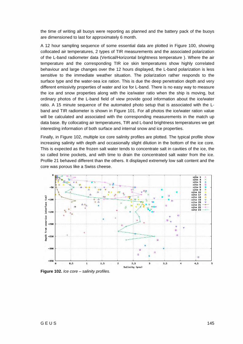
G E U S 145

the time of writing all buoys were reporting as planned and the battery pack of the buoys are dimensioned to last for approximately 6 month.

A 12 hour sampling sequence of some essential data are plotted in Figure 100, showing collocated air temperatures, 2 types of TIR measurements and the associated polarization of the L-band radiometer data (Vertical/Horizontal brightness temperature ). Where the air temperature and the corresponding TIR ice skin temperatures show highly correlated behaviour and large changes over the 12 hours displayed, the L-band polarization is less sensitive to the immediate weather situation. The polarization rather responds to the surface type and the water-sea ice ration. This is due the deep penetration depth and very different emissivity properties of water and ice for L-band. There is no easy way to measure the ice and snow properties along with the ice/water ratio when the ship is moving, but ordinary photos of the L-band field of view provide good information about the ice/water ratio. A 15 minute sequence of the automated photo setup that is associated with the L-band and TIR radiometer is shown in Figure 101. For all photos the ice/water ration value will be calculated and associated with the corresponding measurements in the match up data base. By collocating air temperatures, TIR and L-band brightness temperatures we get interesting information of both surface and internal snow and ice properties.

Finally, in Figure 102, multiple ice core salinity profiles are plotted. The typical profile show increasing salinity with depth and occasionally slight dilution in the bottom of the ice core. This is expected as the frozen salt water tends to concentrate salt in cavities of the ice, the so called brine pockets, and with time to drain the concentrated salt water from the ice. Profile 21 behaved different than the others. It displayed extremely low salt content and the core was porous like a Swiss cheese.

Figure 102. Ice core – salinity profiles.

146 G E U S

16.4 Future Work These more or less synchronous measurements will be gathered in a match up data base after the expedition. The subsequent analysis of data will improve our understanding of snow and sea ice temperatures and the melting/freezing processes in the Arctic. New insight in Arctic snow and ice properties will improve the interpretation of satellite based temperature measurements and eventually result in higher quality temperature data input to ocean and weather models.

16.5 Acknowledgement We wish to thank The Continental Shelf Project of the Kingdom of Denmark, the crew of Oden and all scientist of the LOMROG III expedition for giving us the opportunity to perform this field work in a fine and inspiring environment and with pleasant company.

This research is sponsored by a wide range of national and international R&D projects: EUMETSAT Ocean and Sea Ice Satellite Application Facility (OSISAF), ESA SMOSice and EU cost action SMOS MODE, Greenland Climate and research centre (the Danish Agency for Science, Technology and Innovation), EU MyOcean project, NAACOS project (Danish Strategic Research Council), GHRSST and ESA Climate Change Initiative.

16.6 References Dybkjær, G., Tonboe, R. & Høyer, J. 2012: Arctic surface temperatures from Metop

AVHRR compared to in situ ocean and land data. Ocean Science Discussions 9, 1009–1043, doi:10.5194/osd-9-1009-2012.

Dybkjær, G., Høyer, J., Tonboe, R., Olsen, S., Rodwell, S., Wimmer, W. & Søbjærg, S. 2011: QASITEEX 2011 – The Qaanaaq sea ice thermal emission experiment - Field report. Danish Meteorological Institute Technical Report 11-18 (http://www.dmi.dk/dmi/tr11-18.pdf), 27 pp.

Høyer, J.L., Karagali, I., Dybkjær, G. & Tonboe, R. 2012: Multi sensor validation and error characteristics of Arctic satellite sea surface temperature observations. Remote Sensing of Environment 121, 335-346, doi:10.1016/j.rse.2012.01.013.

Kaleschke, L., Maaß, N., Haas, C., Hendricks, S., Heygster, G. & Tonboe, R. T. 2009: A sea ice thickness retrieval model for 1.4 GHz radiometry and application to airborne measurements over low salinity sea ice. The Cryosphere Discussion 3, 995-1022, doi:10.5194/tcd-3-995-2009.

Tonboe, R.T., Dybkjær, G. & Høyer, J. L. 2011: Simulations of the snow covered sea ice surface and microwave effective temperature. Tellus 63A, 1028-1037, doi: 10.1111/j.1600-0870.2011.00530.x.

Tonboe, R.T. & Hanson, S. 2006: Microphysical measurements important for microwave remote sensing of sea ice - Field guide. Danish Meteorological Institute Scientific Report 06-03 (http://www.dmi.dk/dmi/sr06-03.pdf), 26 pp.

G E U S 147

17. Media on LOMROG III

By Kenneth Sorento (Kenneth Sorento Film & Photography) & Martin Breum, Danish Broadcasting Corporation (DR)

17.1 Introduction The media team included cinematographer Kenneth Sorento and Martin Breum, a journalist with DR, the Danish Broadcasting Corporation. The media team was not formally a part of the LOMROG III-expedition, but invited to cover the expedition and science on board as independent observers. During the cruise, Kenneth Sorento and Martin Breum implemented joint as well as individual projects.

Figure 103. Kenneth Sorento, right, and Martin Breum at the North Pole 22 August 2012.

The team brought its own equipment including an Iridium satellite-connection, on loan from Polaris, for transmission of telephone calls and data. Prior to the expedition certain conditions for media coverage of the expedition were agreed between the Danish Ministry of Education, Science and Innovation and the Danish Broadcasting Corporation. Among other things, it was agreed that:

Privacy on board the icebreaker Oden would be respected

The media coverage should not divulge scientific data from the cruise or interpretations hereof that might harm the Kingdom of Denmark’s negotiating position vis-à-vis the CLCS or neighbouring states

148 G E U S

Media productions should be offered to Swedish broadcasters on normal conditions, since the cruise was a joint Danish-Swedish cruise.

It was also agreed that the Ministry would have the option of screening media material gathered during the cruise to ensure that the agreed conditions were met.

17.2 TV-documentary The main media project was to gather interviews and other TV-material for a 30 minutes TV-documentary on the Continental Shelf Project of the Kingdom of Denmark commissioned by DR, the Norwegian Broadcasting Corporation, NRK, the Greenlandic, KNR, and the broadcaster in the Faroe Island, FVK. The documentary is one of three documentaries on the Arctic commissioned. The final product will be delivered to the broadcasters before 2013.

This production included a number of interviews with scientists and technicians on board, including several with the chief scientist, and with members of the crew.

At an early stage and with the consent of the chief scientists the media team addressed all on board and explained their project and how they intended to go about it. Anyone not willing to appear on TV was asked to say so in order that this wish could be accommodated. No one came forward and it was thus assumed that all on board agreed that they might appear and potentially be identified by television viewers in the planned documentary.

In total six-seven scientists/ technicians from the continental shelf project and 2-3 members of the Oden crew were interviewed for the documentary. They were all informed that their interview would be edited and appear as part of the planned documentary.

17.3 News Coverage The media team produced news coverage for the Danish Broadcasting Corporation, and for KNR, the broadcaster in Nuuk. A background report on the cruise by Martin Breum was published in the Danish newspaper Politiken prior to departure. Also prior to the cruise and at the North Pole the media team facilitated international news coverage of the expedition by Reuters’ news agency.

During the cruise Martin Breum appeared live on radio and TV via satellite-telephone approximately 12 times. Programs included P1Morgen, P3Morgen, Orientering, Deadline and TV-avisen. He also wrote six articles for the webbased news of DR (www.dr.dk/nyheder). The media team also produced an edited radio piece on the cruise that was transmitted to a server at DR in Copenhagen from the Amundsen Basin from a position about 88⁰N.

Twice the media team transmitted edited TV-items for news broadcasts in Denmark. A first item was transmitted to Copenhagen prior to departure from Svalbard. A second 2:30 minutes edited news-piece covering the expedition’s arrival at the North Pole on 22 August 2012 was subsequently broadcast in Denmark, Sweden, Greenland, Finland, Iceland, France and Yemen. The transmission of TV-material from the North Pole entailed moving

G E U S 149

large data files via the media team’s Iridium-connection to a server in Copenhagen. This was not easy, but with a few repeats it worked. It may have been the first time edited TV-material has been transmitted from this latitude.

The successful transmission from the North Pole was reported on by the in-house media within DR (Figure 104).

Figure 104. From DR’s in-house website.

17.4 Other TV-coverage Kenneth Sorento produced several packages of TV-material to other broadcasters in Scandinavia. Footage was shot specifically for “Vetenskapens Värld”, a science program on Swedish SVT.

The Danish web based science hub “Videnskab.dk” and Nordic science website, “ScienceNordic.com” will receive short films about the scientific projects on board.

150 G E U S

Figure 105. Kenneth Sorento shooting on aft deck.

17.5 Other Media Products During the cruise Martin Breum updated his book on Arctic developments and the Danish continental shelf project, “Når isen forsvinder” (“When the Ice Disappears”), to be published in its revised format in early 2013.

Kenneth Sorento and Martin Breum gathered material for an article in the magazine of the Danish Railways, “ud&se”, with one of the larger readerships in Denmark. The article is due to appear in November 2012.

Kenneth Sorento will deliver text and photos for a six pages article on the continental shelf project for “Illustreret Videnskab / Science Illustrated”, the largest popular science magazine in Scandinavia. The article will be published in early 2013.

G E U S 151

Figure 106. Article from Sermitsiaq - a Greenland newspaper, 6 September 2012.

Kenneth Sorento delivered text and photos for an article about the technical challenges in AudioVisuelle Media, a Danish magazine about the film and broadcast industry, and to the web based magazine Iridium 360.

152 G E U S

17.6 Media & Science Relations Only rarely do scientists and media people spend seven weeks on a boat together. In order to learn from this experience and share lessons learned with those interested within the Danish Broadcasting Corporation, Martin Breum conducted a small survey among the scientists of the continental shelf project on board Oden.

The survey was meant as a check on how the scientists perceived their cooperation with the media team. Were they disturbed in their work? Were they comfortable with the media presence? Or did we fail to establish the necessary conditions?

The results of the survey are seen below.

17.7 Survey on Science & Media Relations – with Compiled Results Dear participant on LOMROG III / The Continental Shelf Project: Only rarely do media-people and scientists spend seven weeks on a boat together. We would like to learn from the experience. Please help by answering these ten questions. No need to write your name. Please hand back the form to Martin or Kenneth before Sunday 9.9.The results will be in the media team’s expedition report. Strongly

agree I agree

Don’t know

I Disagree

Strongly disagree

1 The media team was well prepared

4 11 1 1

2 The media team informed me on what they were planning

6 10 1

3 I felt comfortable talking to the media team

6 8 2

4 The media team took an interest in me and my work

3 8 2 3

5 The media team kept me updated on their progress

4 7 3 3

6 The media team listened and adjusted their approach as they learned

1 6 9 1

7 The media team was careful not to inconvenience my work

6 8 2 1

8 The media team made me look at my work in new ways

1 3 12 1

9 The terms of my co-operation with the media team were clear to me

4 10 2 1

10 I trust the media team to publish only what I have agreed to

3 10 4

There was room for additional comment, but only few made any comments. 18 questionnaires were distributed, 17 were returned.

G E U S 153

17.8 Conclusions The media team completed the planned working program during the cruise. News coverage took on unexpected proportions.

Scientists, technicians and crew alike met the many requests from the media team with impressive patience and cooperation. The small science&media survey indicates that most of the scientists had a clear perception of the terms of our cooperation and trusted that we would only publish what was agreed. In retrospect, it might have added to better understanding of the media team if we had:

Clarified the precise nature of our documentary and its three main dramatic flows.

Distributed a small written introduction to our overall plans & terms of cooperation also to crew members.

Media work was greatly facilitated by the chief scientists who readily availed himself and the expeditions’ resources, including a full office container and several helicopter flights.

On-going news coverage took up more time and effort than anticipated. Editors in Copenhagen showed increasing interest in the expeditions as media coverage picked up.

The conditions imposed by the Ministry of Education proved to be only a minor hindrance for coverage of the expedition. It caused no breach of professional ethics. A commitment not to reveal information harmful to the interest of the state differs little from conditions accepted by media working, for instance, with the armed forces during conflict. The media team avoided questions and the filming of conversations that could involve sensitive data. This did not significantly obstruct coverage.

154 G E U S


G E U S 155

18. Acknowledgements

The many results obtained during the LOMROG III cruise could not have been achieved without the excellent cooperation between the crew of Oden, the helicopter crew and the science party. The cooperation between the different science groups made it possible to exploit the resources on board Oden and provided by the helicopter in a very efficient manner.

All members of Oden’s crew, the helicopter crew and the scientific party are thanked for their large commitment for making this cruise so successful.

LOMROG III was the last cruise of the Continental Shelf Project of the Kingdom of Denmark to the area north of Greenland and therefore represents the end of a very successful cooperation between GEUS and the Swedish Polar Research Secretariat. It is hoped that the experience gained during the three LOMROG cruise and the EAGER cruise can be useful for future cruises of Oden to the Arctic Ocean.

156 G E U S


G E U S 157

19. Appendices and Enclosures

19.1 Appendix I: List of Participants Master Erik Andersson Oden Ch. Officer Ivan Öström Oden 2:nd Officer Patrik Johansson Oden 2:nd Officer Kristian Nordström Oden Bosun Lars-Åke Hansson Oden Able Seaman Ralph Björklund Oden Able Seaman Einar Sjöbom Oden Able Seaman Kenneth Nilsson Oden Ch. Engineer Dahn Joelsson Oden 1.st Engineer Jörgen Rundqvist Oden 2:nd Engineer Aron Leth Oden 2:nd Engineer Alexander Hall Oden Oiler Johan Persson Oden Oiler Jonas Lindén Oden Oiler Lennart Pettersson Oden Ch. Cook Lars Andersson Oden Messman Anki Hålldin Oden Cook Peter Ekman Oden Elec. Eng. Jörn Johansson Oden Fitter Per Blad Oden 2:nd Officer Karl Herlin Oden MD Ragnar Jerre SPRS Science Coordinator* Joakim Lindström SPRS SPRS Tech. Erik Hellberg SPRS IT-Tech Björn Eriksson SPRS/ IGV, Stockholm University Hkp. Pilot Sven Stenvall Kallax Flyg, Sikfors, Sweden Hkp. Pilot Arild Ystanes Kallax Flyg, Sikfors, Sweden Hkp. Tech Nils Eriksson Kallax Flyg, Sikfors, Sweden Meteorologist Ulf Christensen SMHI Meteorologist Maria Svedestig SMHI Multibeam op. Nina Kirchner SPRS/ INK, Stockholm University Multibeam op. Rezwan Mohammad SPRS/ IGV, Stockholm University

* for the Swedish research projects

158 G E U S

Chief Scientist Christian Marcussen GEUS Scientist Richard Pedersen KMS Scientist Morten Sølvsten KMS Scientist Thomas Funck GEUS Scientist John Hopper GEUS Scientist Per Trinhammer Geoscience, AU Scientist Simon Ejlertsen Geoscience, AU Scientist Lars Rödel GEUS Scientist Jack Schilling NIOZ Media Martin Breum DR Media Kenneth Sorento DR/ Kenneth Sorento Film & Photography Scientist Richard Gyllencreutz IGV, Stockholm University Scientist Ludvig Löwemark AWI Scientist Pauline Snoeijs Leijonmalm Ecology, Stockholm University Scientist Kajsa Tönnesson BIOENV, University of Gothenburg Scientist Trine Kvist-Lassen GEUS/ Geoscience, AU Scientist Marie Lykke Rasmussen GEUS/ Geoscience, AU Scientist Sofie Ugelvig GEUS/ Geoscience, AU Scientist Markus Karasti IGV, Stockholm University Scientist Peter Sylvander Ecology, Stockholm University Scientist Niki Andersen GEUS Scientist Beatriz Diez Universidad Católica de Chile, Santiago Scientist Laura Farias Universidad de Concepción, Chile Scientist Tanja Stratmann Bioscience, AU Scientist Jerker Eriksson IGV, Stockholm University Scientist Francis Freire IGV, Stockholm University Scientist Indriði Einarsson National Space Institute (DTU-Space) Scientist Thomas Varming BMP Scientist Nikolaj Grønnegaard Vynne National Food Institute (DTU Food) Scientist Brian Sorrell Bioscience, AU Scientist Lars Lund-Hansen Bioscience, AU Scientist Gorm Dybkjær DMI Scientist Steffen Olsen DMI Scientist Rasmus Tonboe DMI AU Aarhus University, Århus, Denmark AWI Alfred Wegener Institute for Polar and Marine Research, Bremerhaven, Germany BIOENV Department of Biological and Environmental Sciences, University of Gothenburg,

Gothenburg, Sweden BMP Greenland Bureau of Minerals and Petroleum, Nuuk, Greenland DMI Danish Meteorological Institute, Copenhagen, Denmark DR Danish Broadcasting Corporation, Copenhagen, Denmark DTU Technical University of Denmark, Lyngby, Denmark Ecology Department of Ecology, Environment and Plant Sciences, Stockholm University,

Stockholm, Sweden GEUS Geological Survey of Denmark and Greenland, Copenhagen, Denmark IGV Department of Geological Sciences, Stockholm University, Stockholm, Sweden INK Department of Physical Geography and Quaternary Geology, Stockholm

University, Stockholm, Sweden NIOZ Royal Netherlands Institute for Sea Research, Texel, Netherlands SMHI Swedish Meteorological and Hydrological Institute, Arlanda/ Norrköping, Sweden SPRS Swedish Polar Research Secretariat, Stockholm, Sweden

G E U S 159

19.2 Appendix II: TPE (Total Propagated Error) – Multibeam Background Information to the settings used in the software during Multibeam Acquisition:

The convention for the Cartesian coordinate system for the EM122 is as follows:

X = Positive Forward

Y = Positive Starboard

Z = Positive Down

The convention for the Cartesian coordinate system for CARIS HIPS/SIPS is as follows:

X = Positive Starboard

Y = Positive Forward

Z = Positive Up

The settings in the rest of this section are just a documentation of the values that were entered into the system during LOMROG-III. A quick examination of these values shows inconsistencies with these numbers. There is also not an obvious way to enter the ship’s physical draught (which was 8.1 meters at the start of the trip). It is a fact that as some of the 4,500 tonnes of fuel is used the draft will decrease significantly. It is reported that the range in draught values due to fuel usage is 6.7 to 8.7 meters.

It also appears that the X & Y values of the MRU to Transducer in the HIPS VCF file have been transposed. This will not affect any sounding positions unless a different sound velocity is re-applied in HIPS.

19.2.1 SIS Installation Settings

Figure 1: Installation parameters: Locations

160 G E U S

Figure 2: Installation parameters: Angular Offset

19.2.2 SeaPath Settings

(Extracted from Configuration Report) Vessel Geometry Vessel dimensions: Length: 107.00 Width: 30.00 Height: 30.00 [m] Center Of Gravity (CG) location: CG-X: -60.00 CG-Y: 0.00 CG-Z: 8.00 [m] Description Vessel data: Type: Ice Breaker Owner: Sjöfartsverket (Swedish Maritime Administration) Name: Oden Country of origin: Sweden Sensor GPS Geometry Antenna Lever Arm From CG to antenna #1: X: 3.973 Y: -3.050 Z: -33.152 [m] GPS Antenna Configuration Baseline length: 2.500[m] Heading offset: -1.68[deg] Height difference: 0.099[m] Attitude Processing Max pitch and roll angles: 15.00 Max average pitch and roll angles: 7.00

G E U S 161

MRU Geometry MRU Lever Arm From CG to MRU: X: 0.000 Y: 0.000 Z: 0.000 [m] MRU Mounting Angles: Roll: -179.77 Pitch: -0.15 Yaw: 0.30 [deg]

19.2.3 Caris HIPS and SIPS

From the VCF (Vessel Configuration File), settings for TPE: Comments Estimated after installation Offsets Motion sensing unit to the transducer 1 X Head 1 17.590 Y Head 1 -2.370 Z Head 1 -9.460 Motion sensing unit to the transducer 2 X Head 2 0.000 Y Head 2 0.000 Z Head 2 0.000 Navigation antenna to the transducer 1 X Head 1 14.860 Y Head 1 -1.500 Z Head 1 -42.600 Navigation antenna to the transducer 2 X Head 2 0.000 Y Head 2 0.000 Z Head 2 0.000 Roll offset of transducer number 1 0.000 Roll offset of transducer number 2 0.000 Heave Error: 0.050 or 0.100'' of heave amplitude. Measurement errors: 0.000 Motion sensing unit alignment errors Gyro:0.000 Pitch:0.000 Roll:0.000 Gyro measurement error: 0.020 Roll measurement error: 0.020 Pitch measurement error: 0.020 Navigation measurement error: 10.000 Transducer timing error: 0.000 Navigation timing error: 0.000 Gyro timing error: 0.000 Heave timing error: 0.000 PitchTimingStdDev: 0.000

162 G E U S

Roll timing error: 0.000 Sound Velocity speed measurement error: 0.000 Surface sound speed measurement error: 0.000 Tide measurement error: 0.000 Tide zoning error: 0.000 Speed over ground measurement error: 0.000 Dynamic loading measurement error: 0.500 Static draft measurement error: 0.000 Delta draft measurement error: 0.500 StDev Comment:

G E U S 163

19.3 Appendix III: Manual for Coring Operation with Dyneema and MacArtney winch on I/B Oden

19.3.1 Winches (see Figure 53 in Chapter 8)

MacArtney MASH 8000/14-90-RA Traction w/ Dyneema (SWL: 9000 kg)

Cormac Oceanographic Winch MASH 5000-10-17Kn (SWL: 1700 kg) on top of MacArtney

Seaproof H07R5D s/n 3565 (SWL: 600 kg) in seismic winch container

19.3.2 Coring Preparations

1. Attach and secure the rail on the aft deck (done by Oden crew). Make sure the necessary blocks are in place in the A-frame (Note! Special plastic block for the MacArtney/Dyneema – see Figure 53). Take care that the sheave of the block for the auxiliary wire has a diameter at least of 250 mm and that it is a wide body block.

2. Attach and secure the cradle onto the rail using the large crane (done by Oden crew). Note! The winged brass screws on the hinged plate under the cradle’s attachment MUST BE OPEN during coring operations (see figure above).

3. Put the lead weights onto the corer head. Full load is 1360 kg (30 x 45 kg or 20 x 68 kg). This goes easier if the corer head is put on one EU-pallet placed upside down on top of another EU-pallet with the lead-end sticking out a bit. Secure it with straps during and after assembly. Attach the lifting hook with 2x2 shackles to the corer head. Put lead weights onto the trigger corer, 1/10 of the weight of the corer (6*22.5 kg = 136 kg on trigger for full weight). Place the piston stop in the connection point for the barrel head.

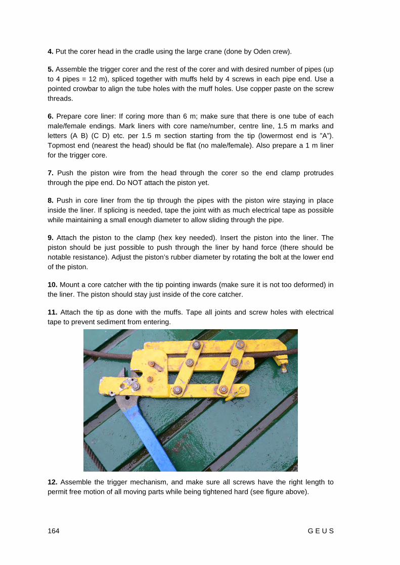
164 G E U S

4. Put the corer head in the cradle using the large crane (done by Oden crew).

5. Assemble the trigger corer and the rest of the corer and with desired number of pipes (up to 4 pipes = 12 m), spliced together with muffs held by 4 screws in each pipe end. Use a pointed crowbar to align the tube holes with the muff holes. Use copper paste on the screw threads.

6. Prepare core liner: If coring more than 6 m; make sure that there is one tube of each male/female endings. Mark liners with core name/number, centre line, 1.5 m marks and letters (A B) (C D) etc. per 1.5 m section starting from the tip (lowermost end is ”A”). Topmost end (nearest the head) should be flat (no male/female). Also prepare a 1 m liner for the trigger core.

7. Push the piston wire from the head through the corer so the end clamp protrudes through the pipe end. Do NOT attach the piston yet.

8. Push in core liner from the tip through the pipes with the piston wire staying in place inside the liner. If splicing is needed, tape the joint with as much electrical tape as possible while maintaining a small enough diameter to allow sliding through the pipe.

9. Attach the piston to the clamp (hex key needed). Insert the piston into the liner. The piston should be just possible to push through the liner by hand force (there should be notable resistance). Adjust the piston’s rubber diameter by rotating the bolt at the lower end of the piston.

10. Mount a core catcher with the tip pointing inwards (make sure it is not too deformed) in the liner. The piston should stay just inside of the core catcher.

11. Attach the tip as done with the muffs. Tape all joints and screw holes with electrical tape to prevent sediment from entering.

12. Assemble the trigger mechanism, and make sure all screws have the right length to permit free motion of all moving parts while being tightened hard (see figure above).

G E U S 165

13. Attach the trigger mechanism to the desired position on the piston wire, usually about 4-6 m from the head (the longer slack, the later start of suction; suction should start at sediment surface).

14. Prepare the trigger rope (from end of trigger arm to trigger corer) with tied nooses at appropriate lengths to permit a desired free-fall height, which should be longer than the piston-wire-slack. IMPORTANT: The parameters free-fall-height and piston-wire-slack determine the start of suction. Divide the trigger rope in two pieces; connect the first piece (2 meter) on the trip-arm. The second pieces should be the length of the head + 6 meter barrel + free-fall (minus 2 meter of first piece). The free-fall length depends of the sediment, stiff sediment need longer free-fall than soft sediment. For extra barrel length, prepare extra 3 meter pieces. To make changing the free-fall easier, prepare pieces of rope with a length of ½ meter, 1 meter and 2 meter. On LOMROG III we used a free-fall between 2.3 and 1.6 meter and a loop between 3 and 6 meters. Take care that you have 2 eyes on the upper part of the second piece, one for connecting to the 2 meter piece, and the second for connection and disconnection to the A-frame.

15. Attach the trigger mechanism to the head’s lifting hook in the slot by the trigger arm. (see figure above). Gather the slacking piston wire to a loose roll and use a little electrical tape to hold the wire slings together. Tie a piece of string around the piston wire and attach it to the shackle that is connected to the head in order to prevent the piston from moving inside the liner before trigger release.

16. Before EACH piston coring: test that the hydrostatic release mechanism can be pushed in with hand force until only about 1 cm sticks out, and that it springs back out the full length again, before attaching it to the trigger mechanism.

166 G E U S

17. Attach the hydrostatic release mechanism to the trigger mechanism. IMPORTANT: Make sure that the screws sit tightly and do not have damaged threads.

18. Important! Attach and keep a long sling connected to the extendable part of the cradle and keep it accessible from the fan tail, so that the lowermost part of the cradle can be uplifted in case Oden needs to run the propellers to push away the ice.

19.3.3 Winch Operations

19.3.3.1 Launching

1. Attach wires: Attach Dyneema to the cradle with a long sling (1.5 m). The sling should stay on the cradle during the entire coring operation. Attach the seismic winch wire to the 2 cradle top holes with a long sling (1.5 m).

2. Move out the cradle: Pull out the cradle slowly (ca 0.1 m/s) by paying in the Dyneema (red) while holding back and paying out continuously with the seismic winch (blue). Stop when the cradle begins to rise. NOTE: Beware of the tension in the Dyneema at all times, because the winches are pulling against each other. If tension goes above 3-4 kN: STOP IMMEDIATELY, then pay out Dyneema. Fill the core liner with sea water to prevent under pressure pushing the piston up when the corer is submerged into the water. Continue to slowly pull out the cradle with the Dyneema (red) while holding back with the seismic winch (blue) until the cradle has reached the rail end and has risen to vertical.

3. Lift the trigger corer with the auxiliary winch and attach it to the cradle using a 2-m rope. Then pay out with the auxiliary winch until slack and disconnect it from the trigger corer. Connect the second part of the trigger rope to the wire of the auxiliary winch and lift the trigger core up, and then move the A-frame out a little so that the trigger core can pass the aft. Payout until the second eye can connect to the cradle, and disconnect the wire. This leaves the trigger weight hanging on the frame.

4. Connect the auxiliary winch to the piston wire (green). Be sure the shackle is connecting on the right way; the shackle into the eye of the piston wire and the bolt into the eye of the auxiliary wire. Pay in the auxiliary winch until the wire is straight up. Connect the

G E U S 167

first eye on the 2 meter piece of the trip arm. Lift up the main core slowly and take care that the core comes out of the cradle and stops when the trigger core is lift up by the main corer via the trip arm. Disconnect the first eye from the cradle. Be sure the whole system is free from the cradle and move out the A-frame so far that the main corer and the trip arm are far enough from the stern. Pay out the auxiliary winch until the connection between auxiliary wire/ piston wire is in a good work height. Move the A-frame in so that you can connect the Dyneema to the piston-core wire eye. Here a Quick link should be used. Pay in the Dyneema a little so that there is tension on the Dyneema. Pay out the auxiliary wire until you can unscrew the bolt of the special shackle. Take of the auxiliary wire and give enough

slack so the A-frame can move out completely. 5. Lift the piston corer out of the cradle using the auxiliary winch.

6. Lower the piston corer until the trigger arm is at a proper working height at Oden’s fan tail. Connect the trigger arm to the trigger core rope while the trigger corer is still hanging

from the cradle. Keep slack on the rope.

7. Connect the Dyneema to the trigger corer, and pay in the Dyneema until it lifts the trigger corer.

8. Pay in with the auxiliary winch until it lifts both piston corer and trigger corer, and there is slack on the Dyneema. Disconnect the Dyneema.

168 G E U S

9. Pay out with the auxiliary winch until the shackle for the piston core wire is at a proper working height. Connect the Dyneema to the piston core wire.

10. Pay in the Dyneema until the auxiliary winch wire is slacking. Disconnect the auxiliary winch wire. You are now ready for coring. Report to Bridge that corer is in the water.

19.3.3.2 Coring

Push out the A-frame and pay out Dyneema to descend the corer to the sea floor. Note the water depth (contact the Bridge via radio). Pay out with about 1.5-1.7 m/s until a few hundred metres from the sea floor. Then slow down to 0.5 m/s until trigger releases (seen as sharp drop in tension and sudden jerk in the Dyneema). Wait a few seconds to let the corer sink in fully. When the corer has reached the sea floor, contact Bridge and note the depth. Slowly (0.3-0.5 m/s) pull out the corer, and note the maximum pull-out tension (usually 25-29 kN). Pay in the Dyneema at about 1.5-1.7 m/s until a few hundred metres from the surface. Then slow down to 0.5 m/s. Stop when the Dyneema’s swivel is visible at the surface. Make sure no ice comes near the Dyneema, which is sensitive to abrasion.

19.3.3.3 Retrieval

1. Connect the auxiliary wire to the piston wire. It is a good idea to mark the Dyneema at 100 meter from the end termination with brightly coloured tape in case the payout indicator is not working properly.

2. Pay out Dyneema until the piston corer hangs in the auxiliary wire. When the connection between the Dyneema and the piston wire is at the right height, move in the A-frame and take care that the Dyneema isn’t damaged by ice floes or the cradle. Connect the auxiliary wire on the eye of the piston core wire. Again be sure the shackle is connected in the right way. Lift the auxiliary wire so that there is tension on the wire. Pay out the Dyneema until the big swivel still is hanging loosely by the Dyneema. Unscrew the quick link and take out the link of the eye of the piston core wire. Pay out enough length of the Dyneema so the A-frame can be moved freely.

G E U S 169

3. Pay in the auxiliary wire until the trigger mechanism is well above the water. Attach the Dyneema to the trigger corer rope. Move out the A-frame until the trip arm and main weight are free from the stern. Pay in the auxiliary wire until the trip arm is on working height. Move the A-frame in so you can work easily on the trip arm. Unscrew the two bolts so that you can take of the trip arm and the moving part. Unscrew the clamp.

4. Pay in the Dyneema until it lifts the trigger corer. Remove the trigger mechanism (wrench needed). Move out the A-frame and pay in the auxiliary wire until the coring head is high enough to fit in to the cradle. Move the A-frame till the core barrel is close to the cradle. Pull the barrel with a rope and move the A-frame inwards slowly to guide the barrel into the cradle. On the starboard side use a wood bar to give extra guiding to the barrel. When the weight is in the right position stop the A-frame. Pay out the auxiliary winch slowly and take care that the weight slides softly into the cradle. Give a little bit extra slack.

5. Pay in Dyneema to lift up the trigger corer on deck. Connect the Dyneema on the free eye of the trigger core rope. Pay in the Dyneema a little bit, so far the tension from the eye connected to the cradle is tension free. Take off the eye and move out the A-frame, so far the trigger core is free from the stern. (Take care the auxiliary winch wire/piston wire has no tension). Pay in the Dyneema and move in the A-frame when the trigger core can come in freely from the aft deck. The trigger weight core is opened and reloaded on the fan tail deck.

6. Pay in auxiliary wire and use the A-frame to lift the piston corer into the cradle.

170 G E U S

7. Pay in on the small winch to raise the cradle in the rail and pull back fully (H).

G E U S 171

19.4 Appendix IV: Core Descriptions1

1 No descriptions are available for LOMROG12-PC10 and for LOMROG12-TC03, 07, 08, 10 & 12, PC – piston core, TC – trigger core.

172 G E U S

G E U S 173

174 G E U S

G E U S 175

176 G E U S

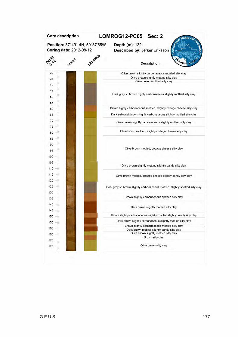
G E U S 177

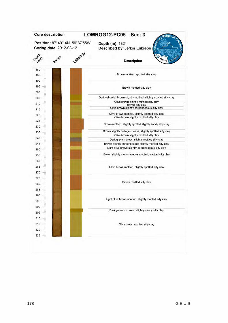
178 G E U S

G E U S 179

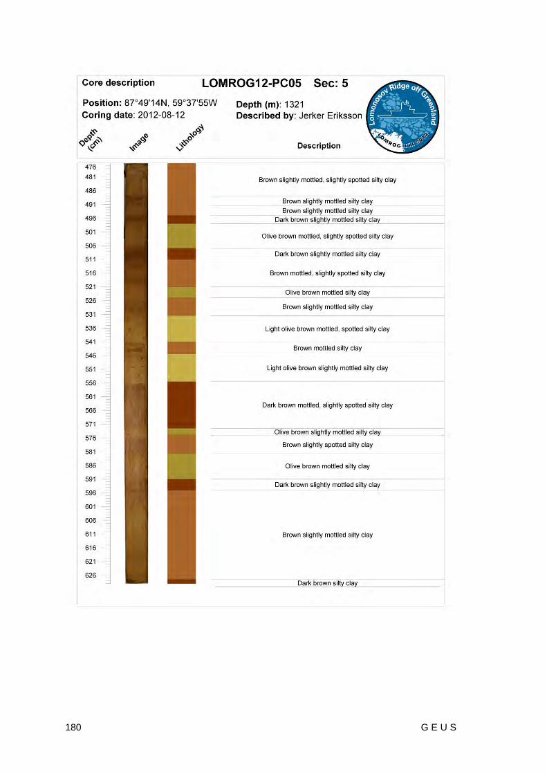
180 G E U S

G E U S 181

182 G E U S

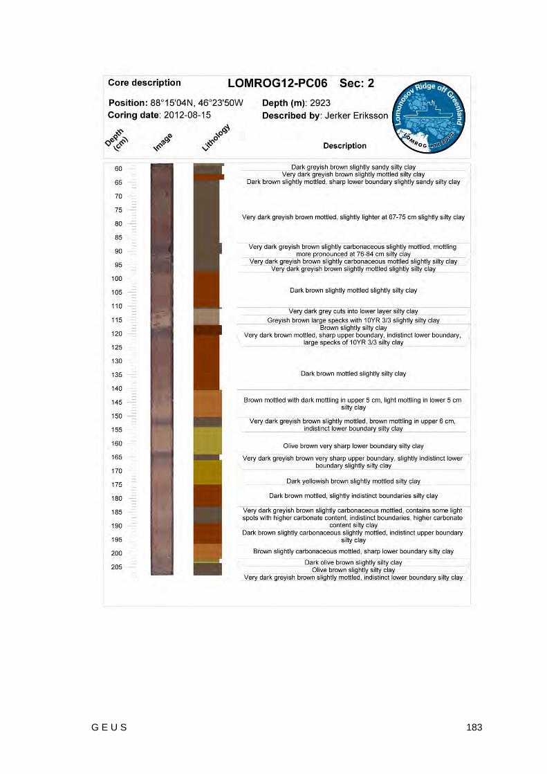
G E U S 183

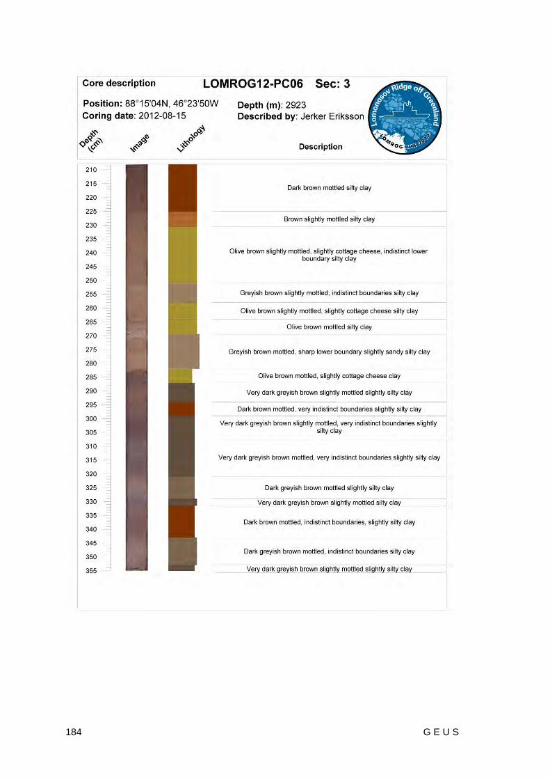
184 G E U S

G E U S 185

186 G E U S

G E U S 187

188 G E U S

G E U S 189

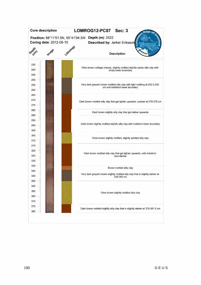
190 G E U S

G E U S 191

192 G E U S

G E U S 193

194 G E U S

G E U S 195

196 G E U S

G E U S 197

198 G E U S

G E U S 199

200 G E U S

G E U S 201

202 G E U S

G E U S 203

204 G E U S

G E U S 205

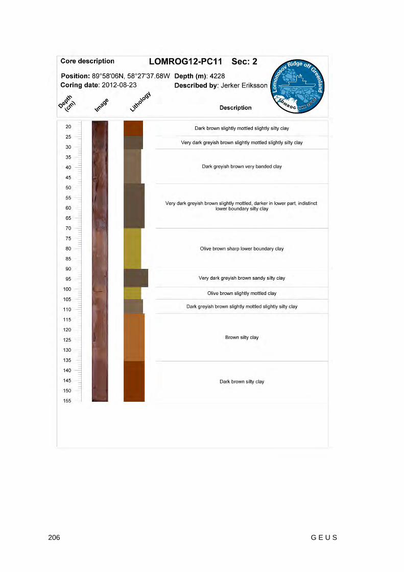
206 G E U S

G E U S 207

208 G E U S

G E U S 209

210 G E U S

G E U S 211

212 G E U S

G E U S 213

214 G E U S

G E U S 215

19.5 Appendix V: Dredging Procedures and Dredging Log Sheets

19.5.1 Dredging Procedures

Dredging procedures developed for LOMROG III

Launching

1. Dredge and weight on the fan tail

2. Connect auxiliary winch to dredge and deploy 500 meters wire (manual level winder needed – two persons)

3. At first end termination connect the weight with chain and shackle

4. Lift weight and pay 12 meter wire out with Aux winch

5. Connect to dyneema

6. Deploy until dredge is at the bottom (pay close attention to the tension meter) - 1 to 1.5 m/sec

7. Pay out 500 meter with the same speed as ship moves until weight is at the bottom – use eventually the ice drift

0.1 knots = 0.05 m/sec 0.2 knots = 0.10 m/sec 0.3 knots = 0.15 m/sec 0.4 knots = 0.21 m/sec 0.5 knots = 0.26 m/sec 0.6 knots = 0.31 m/sec 0.7 knots = 0.36 m/sec 0.8 knots = 0.41 m/sec 0.9 knots = 0.46 m/sec 1.0 knots = 0.51 m/sec 1.1 knots = 0.57 m/sec

8. Pay out at least 1000 meters of dyneema with the same speed as the ship sails or drifts (depends on water depth) – THIS STEP WAS NOT USED DURING THE TWO LOMROG III DREDGES.

2000 to 2500 800 meters 2500 to 3000 1000 meters 3000 to 3500 1200 meters 3500 to 4000 1400 meters

216 G E U S

Dredging and Retrieval

1. Move the ship 0.5 mile

2. Stop the ship as much as possible (might be drifting)

3. Start paying in with 30 meters per minute (0.5 meters per second) until the total cable length is less ( - 100 meters) than the water depth

4. Start paying in with 60 to 90 meters per minute (1.0 to 1.5 meters per second)

5. Connect the Aux winch and disconnect the dyneema

6. When the weight is coming up use the seismic winch to place the weight on the fan tail and disconnect it

7. Pay in 500 meters using the Aux winch

8. Lower the dredge on fan tail with A-frame and Aux winch

9. Check the content of the dredge on the fan tail

NO OTHER PEOPLE ALLOWED ON AFT DECK WHILE DREDGING

Person on the aft deck during deployment Fan tail: Jack and Lars

Aux winch: Per (two person for the level winder)

Geo winch: Erik (on deck with remote control), Per can take over

A-frame: Ivan

Persons on the aft deck during recovery Fan tail: first only Jack (disconnect dyneema and connect the weight on the seismic winch and place it on the aft deck), later with Lars (to assist retrieval of the dredge)

Aux winch: Per/Lars (two persons for the level winder)

Seismic winch: Lars

Geo winch: Erik (in the geo winch container to adjust level winder), Per

A-frame: Ivan

Communication between aft deck and bridge:

Per communicates with the bridge on VHF.

Jack is in command on the aft deck.

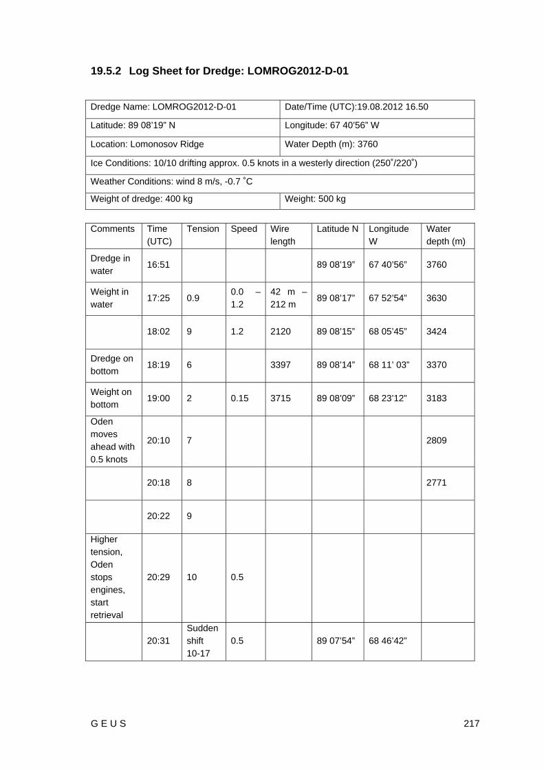
G E U S 217

19.5.2 Log Sheet for Dredge: LOMROG2012-D-01

Dredge Name: LOMROG2012-D-01 Date/Time (UTC):19.08.2012 16.50

Latitude: 89 08’19” N Longitude: 67 40’56” W

Location: Lomonosov Ridge Water Depth (m): 3760

Ice Conditions: 10/10 drifting approx. 0.5 knots in a westerly direction (250˚/220˚)

Weather Conditions: wind 8 m/s, -0.7 ˚C

Weight of dredge: 400 kg Weight: 500 kg

Comments Time

(UTC) Tension Speed Wire

length Latitude N Longitude

W Water depth (m)

Dredge in water

16:51 89 08’19” 67 40’56” 3760

Weight in water

17:25 0.9 0.0 – 1.2

42 m – 212 m

89 08’17” 67 52’54” 3630

18:02 9 1.2 2120 89 08’15” 68 05’45” 3424

Dredge on bottom

18:19 6 3397 89 08’14” 68 11’ 03” 3370

Weight on bottom

19:00 2 0.15 3715 89 08’09” 68 23’12” 3183

Oden moves ahead with 0.5 knots

20:10 7 2809

20:18 8 2771

20:22 9

Higher tension, Oden stops engines, start retrieval

20:29 10 0.5

20:31 Sudden shift 10-17

0.5 89 07’54” 68 46’42”

218 G E U S

20:43 2690

20:46 Fairly stable 10-11

89 07’54” 68 49’32” 2661

20:55 11 3000 89 07’52” 68 51’11” 2599

Weight off bottom

21:19 Stable 11

2280 89 07’47” 68 55’27” 2475

Dredge off bottom

21:28 10 1.5 2020 89 07’45” 68 57’11” 2424

21:39 1000 89 77’42” 68 59’34” 2357

Dyneema at surface

21:50 76 89 07’40” 69 01’38” 2261

Weight out of water

22:02 89 07’37” 69 03’55” 2170

Dredge on deck

22:19 89 07’32” 69 07’10” 2032

Estimate of material in dredge: 100 kg + Number of sample bags: 12

G E U S 219

19.5.3 Log Sheet for Dredge: LOMROG2012-D-02

Dredge Name: LOMROG2012-D-02 Date/Time (UTC):20.08.2012 11.26

Ships speed: 0.5 knots in a southerly

direction Water Depth (m): 3760

Weight of dredge: 400 kg Weight: 500 kg

Comments Time

(UTC) Tension Speed

Wire length

Latitude NLongitude W

Water depth (m)

Dredge in water

11:26 89 17’42” 60 08’16” 3853

Weight in water

11:43 9 9

1.0 1.2

130 250

89 17’35” 60 06’33” 3725

12:24 3100 89 17’12” 60 04’08” 3495

Dredge on bottom

12:35 6 3530 89 17’07” 60 04’10” 3466

Weight on bottom

13:07 4 4033 89 16’50” 60 05’42” 3326

Dredge 13:34 5 89 16’37” 60 08’05” 3164

Dredge 13:48 6 89 16’31” 60 09’32” 3108

14:05 7 89 16’23” 60 11’41” 3011

14:08 8-9 0.1 – 0.5

89 16’22” 60 12’07” 2984

14:09 7-8 0.5 4000 2896

14:09 13! 2983

14:12

20-21-22-23, 27. Peak at 28

89 16’20” 60 12’36” 2815

220 G E U S

Weight off bottom

14:12 9 0.3 89 16’20” 60 12’42” 2880

Dredge still on sea bottom Tension 9-10, varies with 3 kN

14:16 9-10 -> 13

2931 very unstable depth from MB

14:23 12 3600 2859

15:08 11 0.3 2300 2623

15:15 11

Increasing from 0.3 to 1.5

2000 89 15’55” 60 20’37” 2607

No change in tension, not clear when dredge left sea bottom

15:18 13 1.5 1800 89 15’54” 60 21’04” 2586

15:32 12 760 89 15’49” 60 22’35” 2433

Dyneema at surface

15:38 98 89 15’47” 60 23’30” 2511

Weight out of water

15:48 89 15’43” 60 24’43” 2517

Only steel wire left

15:53

Dredge on deck

16:08 89 15’37” 60 26’56” 2463

Estimate of material in dredge: 200 kg + (a lot of mud) Number of sample bags: 10 + 1 large stone

Documents

Lomonosov Ridge off Greenland 2012 (LOMROG III) – Cruise ... · Geological Survey of Denmark and Greenland Bulletin 4, 61–64. Marcussen, C. & Heinesen, M. 2010: The Continental