Embed Size (px)
Citation preview

“LOGISTICS MODELS”
Andrés Weintraub P.
Departament Industrial EngineeringUniversity of Chile
PASISantiago
Agosto 2013
IFORS Hawaii, July 2005

Column Generation Combined with Constraint Programming to Solve a
Technician Dispatch Problem
Cristián E. CortésCivil Engineering Department
Andrés WeintraubSebastián Souyris
Industrial Engineering DepartmentUniversity of Chile
Michel GendrauEcole Polytechnique, Montreal

Motivation
• Real Problem: Dynamic dispatch of technicians of Xerox Chile to repair failures of their machines along the day.
• The proposed scheme is based upon the classic formulation of the Vehicle Routing Problem with Soft Time Windows (VRPSTW), and it is formulated and solved as a Dantzig-Wolfe decomposition by using column generation along with classical insertion heuristics, under a constraint programming approach.
• Xerox strategic objective: Client satisfaction, so technical service becomes relevant
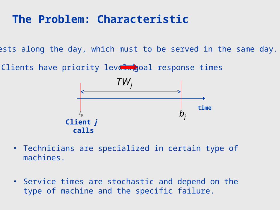
The Problem: Characteristic
• Technicians are specialized in certain type of machines.
• Service times are stochastic and depend on the type of machine and the specific failure.
0t
Client j calls
time
•Requests along the day, which must to be served in the same day.
•Clients have priority levels goal response times
jTW
jb

IFORS Hawaii, July 2005
The problem
• The objective function for assigning technicians and jobs is to minimize two components:
– the sum of the differences between goal response times of clients and the effective service time provided by Xerox
– the sum of travel times.


Approaches
• Based on queuing theory– Dynamic Traveling Salesman Problem (Psaraftis,1988)
– Dynamic Traveling Repairman Problem (Bertsimas et. al.,
1991)
• Algorithmic– Analytical Models
– Heuristics and Metaheurstics
• Tabu Search (Gendreau et. al., 1999), Ant Colony System (Montemanni, 2002).
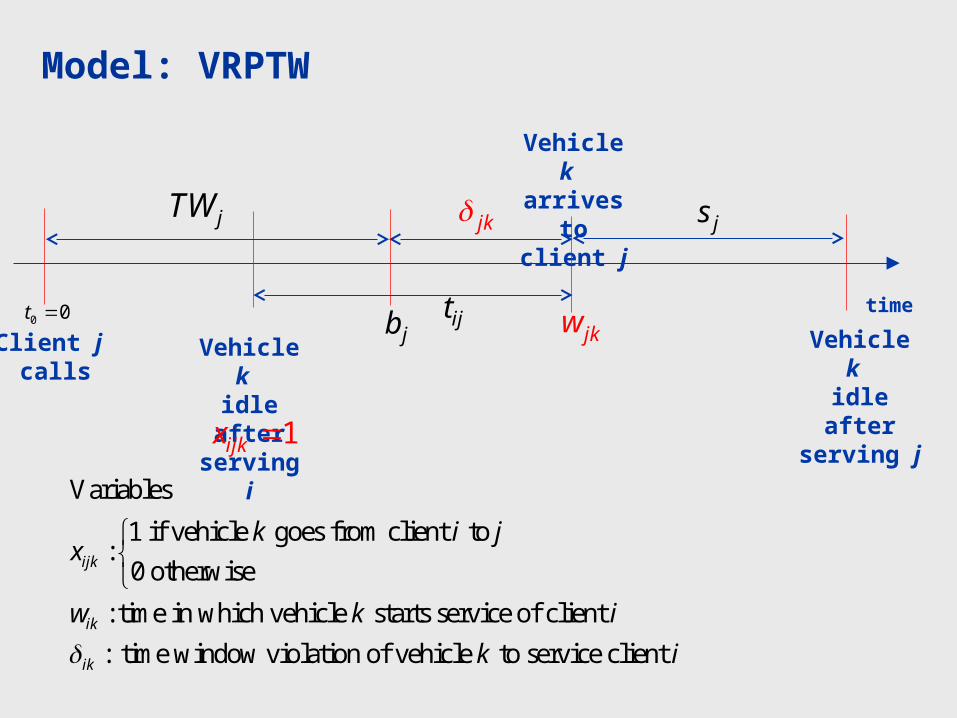
Model: VRPTW
time
Vehicle k idle after serving i
jTW
Vehicle k idle after serving j
Client j calls
0 0t
jk js
jb
Vehicle k arrives to
client j
jkwijt
1ijkx
Variables
1 if vehicle goes from client to :
0 otherwise
: time in which vehicle starts service of client
: time window violation of vehicle to service client
ijk
ik
ik
k i jx
w k i
k i

1 2 2
, , 2
0,1 , ,
, 0 ,
kij
i k i k
x i I I j I k K
w i I k K
UNature of Variables
OF: Minimize TW violation and travel time
,,
min (1 ) kx ik ij ij
k K i I k K i j I
t x
1 2 2
21
,0k kij ji
i I I i I I
j k Kx x I
U U
Flow Conservation
:Multi Objective Parameter
1 21kij
k K j I
x i I I
UEach customer must be served
1 2 2(1 ) * , ,
, , : latest arrival time
,
kik i ij jk ij
kik ji
j I
ik ik i
w s t w x M i I I j I k K
w F x i I k K F
w b i I k K
U
Temporal and feasibility constraints
Path ends in the final fictitious technician
1 2
1 1kiI
i I I
x k K
U

Master ProblemSet Partitioning
Model
COLUMN GENERATORSub Problem
: min
1
{0,1},
r r
xr R
r ri
r R
r
P c x
a x i I
x r R
Dual
Multipliers
Columns
i
,
Reduced Cost Column
kk kk ki ij
i P i j Pi
i P
c t
Reformulation
Constraint Programming
¿ * 0?rc

IFORS Hawaii, July 2005
Description of the General Process
1. Generate a set of initial routes, feasible problem.
2. Solve a linear relaxation of the master problem with the generated pool of routes.
3. From the dual variables associated to the constraints of each machine in the master problem, generate the route with minimum reduced cost (subproblem). If its reduced cost cr*<0 , go to 4, otherwise go to 5.
4. Using the sub-problem generate all possible columns with reduced cost less than and length L, where is a control parameter that satisfies , thus
. Go to 2.
5. Solve MP using B&B including all the columns generated in the previous steps, obtaining the final routes to be followed by each technician.
*cr 0 1
[ *, * ] 0cr cr cr

IP Model v/s CG
• Instance: 5 technicians, 20 clients• IP Model: optimal solution in 3.5 hrs.• CG: optimal solution in 15 iterations, 3.7 sec.
Model coded with ILOG Concert Technology, and solved by using CPLEX 9.0 and SOLVER 6.0
0
5
10
15
20
25
30
35
40
45
0 5 10 15 20 25 30 35 40 45 X
YObjective Funcion / Iteration
0
20
40
60
80
100
120
140
160
180
200
1 2 3 4 5 6 7 8 9 10 11 12 13 14 15
Column Generation
Exact ModelOptimal Solution
Number of Iterations
Example Real Instance
• Real Operation: Normal working day, 36
clients,9 technicians
• Optimization total time 500 sec.
• The following maps show observed routing
versus optimized routing.

Real instance

1
7
227
620
3
4
5
9
1017
14
23
3233
16
18
21
22
3625
28
29
31
34
15
26
13
19
35
24
8
11 30
12

1 2 2
2
0,1 ,
, 0
ij
i i
x i I I j I
w i I
UNature of Variables
OF: Minimize reduced cost
2 1 2, ,
, ,
min (1 )i ij ij i ijx w
i I i j I I k K i j I
t x x
1 2 2
21
0ij jii I I i I I
jx x I
U U
Flow Conservation
1 2
1iji I j I
x
One technician follow the new path
1 2
1 2 2
2
2
(1 ) * ,i i ij j ij
i jij I I
i i i
w s t w x M i I I j I
w F x i I
w b i I
U
UTemporal and
feasibility constraints
Path ends in the final fictitious node
SP: Shortest Path Problem With Soft Time Windows
1 2
1 1iIi I I
x
U

17
How to solve it?
• Dynamic Programming:– The most used approach in literature.– Difficult to implement and solve it under Branch
and Price scheme.
• Constraint Programming:– Good performance for short routes.– Easy to implement and solve it under Branch and
Price scheme with Constraint Branching.

7
227
620
3
4
5
9
1017
14
23
3233
16
18
21
22
3625
28
29
31
34
15
26
13
19
24
8
11 30
121
35
Actual Path

1
7
227
620
3
4
5
9
1017
14
23
3233
16
18
21
22
3625
28
29
31
34
15
26
13
19
35
24
8
11 30
12
OPT Path

OPT PATHS REAL PATHSPath Maq w d s trm tv Path Maq w d s trm tv
1 m1 755 0 60 755 0 1 m2 660 0 120 1002 19m20 838 73 30 765 23 m3 810 0 180 1015 30m17 892 0 80 929 24 m27 1680 0 30 2040 30m34 993 0 90 1059 21 m34 1800 741 90 1059 0m36 1109 0 145 1890 26 2 m4 1670 648 100 1022 20
2 m2 1002 0 120 1002 0 m36 2085 53 70 2032 22m15 1152 0 120 1716 30 m32 1820 0 145 1890 26m32 1290 0 70 2032 18 3 m18 870 0 50 970 0m26 1371 0 180 1652 11 m21 930 0 60 947 0m16 1581 0 120 1718 30 4 m9 1020 0 60 1068 30
3 m4 1022 0 100 1022 0 m15 1710 0 120 1716 60m10 1152 307 85 845 30 m16 1860 142 120 1718 17m21 1262 315 60 947 25 5 m20 1665 3 75 1662 15m30 1354 0 150 1893 32 m17 1770 0 90 1834 20
4 m5 1024 0 45 1024 0 m29 910 0 80 929 20m31 1083 0 90 1780 14 m12 765 0 30 765 0m22 1190 0 120 1832 17 m14 1020 0 60 1955 20m11 1325 0 40 1779 15 m31 1980 200 90 1780 40
5 m6 1980 0 60 1980 0 6 m10 1665 641 45 1024 15m23 2068 0 20 2250 28 m5 720 0 85 845 30m33 2113 0 60 2214 25 m28 1980 201 40 1779 60
6 m8 943 0 135 943 0 m22 1800 0 120 1832 15m19 1101 116 120 985 23 m11 1740 39 30 1701 30m13 1244 245 60 999 23 m33 2130 0 60 2214 42m28 1352 0 30 1701 48 7 m7 900 145 60 755 41m35 1425 0 90 2010 43 m1 600 0 195 805 14
7 m9 1068 0 60 1068 0 m25 990 0 90 1651 18m14 1143 0 90 1834 15 m26 1650 0 180 1652 0m25 1244 0 90 1651 11 8 m6 990 0 60 1980 20
8 m12 1662 0 75 1662 0 m23 990 0 20 2250 30m27 1761 0 30 2040 24 m30 1680 0 150 1893 30m29 1812 0 60 1955 21 9 m8 705 0 135 943 10
9 m18 970 0 50 970 0 m13 930 0 60 999 20m3 1045 30 180 1015 25 m19 1800 815 120 985 150m7 1249 444 195 805 24 m24 1995 237 105 1758 15m24 1474 0 105 1758 30 m35 2110 100 90 2010 10TOTAL 1530 656 TOTAL 3965 918
Z* 3716 Z* 8848

But, this procedure doesn’t assure optimality…
• Improve CG methodology: Branch and Price. – Previous methodology does not ensure optimality– When descending along the B&B tree, new routes with
negative reduced cost could be found– B&P: Generate columns at each node of the Branch &
Bound– Columns generated at each node have to be consistent
with the partition associated to such a node
• First Approach using Maestro Library for B&P (ILOG).– Same Master Problem.– Sub Problem with IP Shortest Path Model. =>only
solves medium instance (40 clients 10 technicians) in prohibited computational time.

• Second Approach B&P– Same Master Problem.– Sub Problem with :
• Ryan and Foster (1981) Branching Strategy.
1. Constraint Programming.2. Dynamic Programming.
(Shortest Path with Soft Time Windows)
Wich one is better?
Objective Function GAP Objective Function CPU TimeInstance RL CG B&P GAP RL-CG GAP B&P-CG CG B&P
[nCl_nTec(nInst)] [%] [%] [seg] [seg]20_5(1) 729 729 729 0 0 5 110620_5(2) 139 141 141 1 0 4 11920_5(3) 108 108 108 0 0 5 2220_5(4) 99 99 99 1 0 2 1130_6(1) 207 216 216 4 0 102 2425
30__6(2) 164 192 173 15 10 227 356430_6(3) 258 258 258 0 0 54 159330_6(4) 170 170 170 0 0 160 1137
40_10(1) 705 705 705 0 0 141 3997840_10(2) 633 634 634 0 0 110 3369740_10(3) 192 202 195 5 3 116 262840_10(4) 202 206 204 2 1 78 3835
23
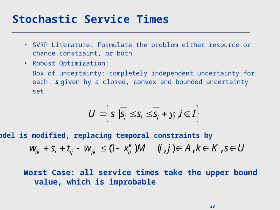
Stochastic Service Times
• SVRP Literature: Formulate the problem either resource or chance constraint, or both.
• Robust Optimization:
Box of uncertainty: completely independent uncertainty for each si given by a closed, convex and bounded uncertainty set
| , i i i iU s s s s i I
Worst Case: all service times take the upper bound value, which is improbable
Model is modified, replacing temporal constraints by
(1 ) ( , ) , ,kik i ij jk ijw s t w x M i j A k K s U

24
Stochastic Service Times
Worst Case: for each route, first clients complete their repair time until Uk
(Optimal solution of Robust problem has variations in service times as early as possible, which was analytically proved and it is also a very intuitive result)
Independent service time uncertainty per technician
robust parameter:
kk i
i P
U
( )
routing solution
( ) | , ,
:
kr
r i i i ik ik ki P x
r r
U x s s s s z i I z U
x

2 1 2, 1
parameter for control uncertainty:
kik ij i
i I i I j I I
k Kz x
U
Max Service Time above average by technician
1 2
kik i ji
j I I
k Kz y
U
Max Service Time above average by client
1 2, 1 ,k kij ij i I j I k Ky x I U
Relation between variables x and y
1 2 2
, , 2
0,1 , ,
, 0 ,
kij
i k i k
x i I I j I k K
w i I k K
U
1 2 2
21
,0k kij ji
i I I i I I
j k Kx x I
U U
1 21kij
k K j I
x i I I
U
2 2 2
end of the day
(1 ) *
, ,
, , :
,
kik i ik ij jk ij
kik ji
j I
ik ik i
w s z t w x M
i I I j I k K
w L x
i I k K L
w b i I k K
U
1 2
1 1kiI
i I I
x k K
U
,,
min (1 ) kx ik ij ij
k K i I k K i j I
t x
Two new Variables:
20ikz i I Upper value for client i service time
1 2 2
0,1
,
ijy
i I I j I
U
If previous client has max service time
1 2, 1 ,k ikij
ii I j I k K
zy I U
Relation between variables z and y
Model forces to have repair time of max length at the beginning of each route (worst case).

• Characteristic of the problem
• Mathematical Model
• Decomposition approach
• Robust approach
• Robust results
• Conclusions

27
Robust Model Test
• New constraints are added to the SubProblem.
• Test: – Comparison with deterministic model. – Real data. – For each customer, assume Weibell distribution (which
represents repair times properly). Parameters for Weibell, derived from data. Obtain 1000 values of repair time for each customer, leading to 1000 simulations.
– For each instance we test different values.
• Experiments consider sensitivity in standard deviation associated with real data

sSimulado(M77,std22)
Av(twv)
50
70
90
110
130
150
0 0.3 0.6 0.9
0.3
0.6
0.9
Av(of)
0
100
200
300
400
500
600
0 0.3 0.6 0.9
0.3
0.6
0.9
StD (twv)
100
105
110
115
120
125
130
0 0.3 0.6 0.9
0.3
0.6
0.9
robust parameter
: m
:
ulti objective parameter
k
k ii P
U

sSimulado(M77,std70)Av(twv)
400
700
1000
1300
0 0.3 0.6 0.9
0.3
0.6
0.9
Av(of)
500
600
700
800
900
1000
1100
0 0.3 0.6 0.9
0.3
0.6
0.9
StD (twv)
600
700
800
900
1000
1100
1200
0 0.3 0.6 0.9
0.3
0.6
0.9

• Characteristic of the problem
• Mathematical Model
• Decomposition approach
• Robust approach
• Robust results
• Conclusions

31
Conclusions and Further Research
• Robust Model represent quite well the worst case, easy to
implement and give better results than determinist model.
• Benefits of the robust model strongly depend on the variability of
the real data uncertainty.
• CP allows to easily implement the Robust model under the same
B&P algorithm developed for the deterministic case
• Dynamic Routing, Fleet design

• If a column is created:
– Incorporate constraint: this new column can´t be created again into the subproblem.
• Solver Search:
– Dichotomic strategic.
– Procedure: depth first search.
• How many columns must be generated at each
iteration?
• Under which criteria?

5. Time to begin the service
SC[l-1] SC[l-1],SC[1]w[l]= w[l-1]+s +t , l = 1..L
6. Violation of time windows
SC[l]d[l]= MAX(0,w[l]- b ) , l = 1..L
4. Initial Conditions
w[0]= 0, d[0]= 0
2. All the clients in the path must be different:
alldifferent[SC]
1. First client in the path must have technician and the others no:
,
SUBJECT TO
1 2 3SC[0] I SC[l] I I l = 1..L
8. Negative Reduced Cost
) 0 SC[l-1],SC[l] SC[l]l l l
* d[l]+(1- t -
3. If client is fictitiuos then also:
, 3 3
l l+1
SC[l] I SC[l+1] I l = 1..L-1
7. Relation between and variables
i I
SC a
a[SC[l]]= 1 , l = 1..L
a[i]= L
VARIABLESSC[l] I: secuence of clients in path, l = 0..L
w[l] [0..F] : time to begin service of client l = 0..L
d[l] [0..F] : time windows violation of client l = 1..L
a[i] {0,1}: 1 if client i is in path, 0 otherways
Constraint Programming Model
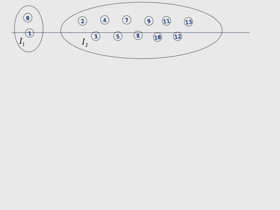
1I
0
1
2I
2
3
4
5
7
8
9
10
11
12
13

1I
0
1
2I
2
3
4
5
7
8
9
10
11
12
13

SC[0]= 0
1I
0
1
2I
2
3
4
5
7
8
9
10
11
12
13

1I
0
1
2I
2
3
4
5
7
8
9
10
11
12
13
SC[0]= 0
SC[1]= 2

1I
0
1
2I
2
3
4
5
7
8
9
10
11
12
13
SC[0]= 0
SC[1]= 2
SC[2]= 3

1I
0
1
2I
2
3
4
5
7
8
9
10
11
12
13
SC[0]= 0
SC[1]= 2
SC[2]= 3
SC[3]= 4SC[2]= 3

1I
0
1
2I
2
3
4
5
7
8
9
10
11
12
13
SC[0]= 0
SC[1]= 2
SC[2]= 3
SC[3]= 4SC[3]= 5
SC[4]= 7SC[4]= 8

1I
0
1
2I
2
3
4
5
7
8
9
10
11
12
13
SC[0]= 0
SC[1]= 2
SC[2]= 3
SC[3]= 4SC[3]= 5
SC[4]= 7SC[4]= 8
SC[5]= 9SC[5]= 10
Feasible Route!
)
1
l
SC[l-1],SC[l]l
Z = * d[l]+
(1- t 1
add constraint
for next solutions:
Z < Z

1I
0
1
2I
2
3
4
5
7
8
9
10
11
12
13
SC[0]= 0
SC[1]= 2
SC[2]= 3
SC[3]= 4SC[3]= 5
SC[4]= 7SC[4]= 8
SC[5]= 9SC[5]= 10
a[0]= a[2]= a[3]=
a[5]= a[8]= a[10]= 1;
a[4]= a[7]= a[9]=
a[11]= a[12]= a[13]= 0
Reconstruct the pathwith this nodes.

SC[0]= 0
SC[1]= 2
SC[2]= 3
SC[3]= 4SC[3]= 5
SC[4]= 7SC[4]= 8
SC[5]= 9SC[5]= 10
a[0]= a[2]= a[3]=
a[5]= a[8]= a[10]= 1;
a[4]= a[7]= a[9]=
a[11]= a[12]= a[13]= 0
1I
0
1
2I
2
3
4
5
7
8
9
10
11
12
13
SC[0]= 0
SC[1]= 3
SC[2]= 8
SC[3]= 5
SC[4]= 2
SC[5]= 10
'11Z Z

In each iteration of column generation :
Let SP general subproblem, SP' subproblema with a variable fixed,
Start New Search for SP;
while (SP find new solution){
solve SP' with a obtained for the actual solution of SP ;
add new column to MP;
}
end search SP;

Branching Strategy: Constraint Branching (Ryan and Foster)
If a basic solution is fractional then there exist two clients i and j such that:
: 1, 1
0 1r ri j
rr a a
because every column must be different.
Then the branching constraints are the clients i and j have to be covered: Left branch by the same columnRight branch by different columns
min
1
{0,1},
r r
xr R
r ri
r R
r
c
a i I
r R
Master Problem:

Branching Strategy: Constraint Branching (Ryan and Foster)
i
j
i
j
i
j
i
j
Two type of columns Three type of columns
i
j

47
Ryan and Foster (1981) branching strategy: benefits
• All constraints are imposed at the sub-problem directly
• B&B terminates after a finite number of branches since
there are only a finite number of pairs of rows.
• Each branching decision eliminates a large number of
variables from consideration .

Example Real Instance
• Real Operation: Normal working day, 36 clients,9
technicians
• Optimization total time 100 sec.
• The following maps show observed routing versus
optimized routing.


Path used by the firm

3
Path in Column Generation

CG Firm CG Firm CG Firm
1530 3965 656 918 1268 3051
Z*Travel timeViolation
= 0.7

53
Computational Results
CPU TimeInstance LR CG B&P LR-CG B&P-CG CG
[nC_nTec(nInst)] [%] [%] [sec]40_10(1) 705 705 705 0.00 0.00 141.3240_10(2) 633 634 634 0.16 0.00 110.2940_10(3) 192 202 195 4.86 3.47 115.9940_10(4) 202 206 204 2.06 0.98 77.5350_10(1) 1337 1337 1337 0.00 0.00 381.01650_10(2) 1865 1879 1879 0.75 0.00 284.82850_10(3) 1513 1523 1523 0.69 0.00 369.12550_10(4) 1727 1745 1745 1.04 0.00 517.53170_10(1) 1581 1631 1631 3.04 0.00 3411.1470_10(2) 904 940 940 3.83 0.00 3253.8670_10(3) 226 233 233 2.86 0.00 3550.95
LR: Linear RelaationCG: Column GenerationB&P: Branch and Price
Objective Function GAP Objective Function

Histograma B = 9 (fo(0) - fo(0.6))
0
20
40
60
80
100
120
140
160
180
200
-400 -340 -280 -220 -160 -100 -40 20 80 140 200 260 320 380 440
Clase
Fre
cuen
cia

Constraint Programming Model
2I1I
3 5 10 14 17 21
3
5
10
14
17
21
SC[0] SC[1] SC[2] SC[3] SC[4] SC[5]

Constraint Programming Model
2I1I
3 5 10 14 17 ?
3
5
10
14
17
SC[0] SC[1] SC[2] SC[3] SC[4] SC[5]

Constraint Programming Model
2I1I
3 5 10 14 ? ?
3
5
10
14
SC[0] SC[1] SC[2] SC[3] SC[4] SC[5]

Constraint Programming Model
2I1I
3 5 10 14 ? ?
3
5
10
14
n+1
n+2
n+3
n+4
Fictitious nodes
3I
SC[0] SC[1] SC[2] SC[3] SC[4] SC[5]

Constraint Programming Model
2I1I
3 5 10 14 n+1 n+2
3
5
10
14
SC[0] SC[2] SC[3] SC[4] SC[5] SC[6]
n+1
n+2
n+3
n+4
Fictitious nodes
3I


![[Steven h. weintraub]_jordan_canonical_form_appli(book_fi.org)](https://img.pdfslide.us/doc/110x75/55d6bdbdbb61ebe1698b464a/steven-h-weintraubjordancanonicalformapplibookfiorg.jpg)