1

Logistic RegressionPart 1

2

The exponential function exp(x) = ex plays a fundamental role in logistic

regression and in many other branches of mathematical modelling, machine

learning and data science.

When x tends to -∞ the exponential tends to 0.

When x tends to 0 the exponential tends to 1.

When x tends to +∞ the exponential tends to +∞.

The exponential function

3

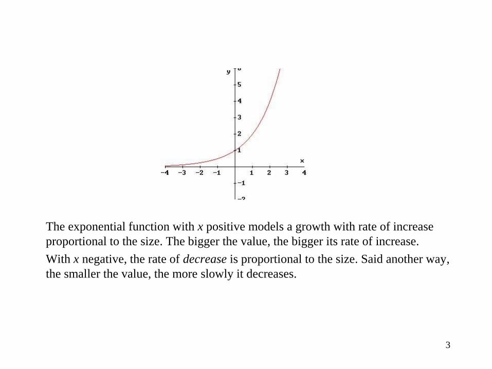
The exponential function with x positive models a growth with rate of increase

proportional to the size. The bigger the value, the bigger its rate of increase.

With x negative, the rate of decrease is proportional to the size. Said another way,

the smaller the value, the more slowly it decreases.

4

The logarithmic function log(x) is the inverse of the exponential function:

log exp 𝑥 = exp log 𝑥 = 1

When x tends to 0 the logarithm tends to -∞.

When x tends to 1 the logarithm tends to 0.

When x tends to +∞ the logarithm tends to +∞.

The logarithmic function

5

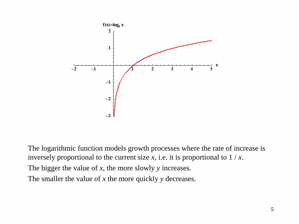
The logarithmic function models growth processes where the rate of increase is

inversely proportional to the current size x, i.e. it is proportional to 1 / x.

The bigger the value of x, the more slowly y increases.

The smaller the value of x the more quickly y decreases.

6

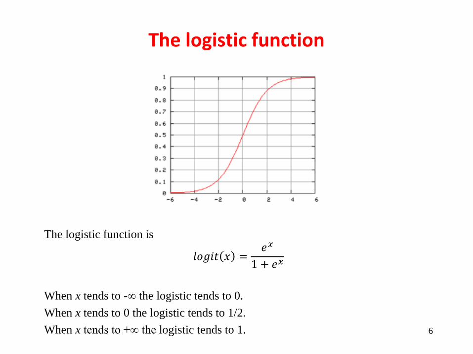
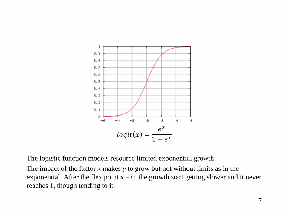
The logistic function is

𝑙𝑜𝑔𝑖𝑡 𝑥 =𝑒𝑥

1 + 𝑒𝑥

When x tends to -∞ the logistic tends to 0.

When x tends to 0 the logistic tends to 1/2.

When x tends to +∞ the logistic tends to 1.

The logistic function

7

𝑙𝑜𝑔𝑖𝑡 𝑥 =𝑒𝑥

1 + 𝑒𝑥

The logistic function models resource limited exponential growth

The impact of the factor x makes y to grow but not without limits as in the

exponential. After the flex point x = 0, the growth start getting slower and it never

reaches 1, though tending to it.

8

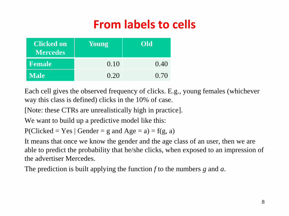
Each cell gives the observed frequency of clicks. E.g., young females (whichever

way this class is defined) clicks in the 10% of case.

[Note: these CTRs are unrealistically high in practice].

We want to build up a predictive model like this:

P(Clicked = Yes | Gender = g and Age = a) = f(g, a)

It means that once we know the gender and the age class of an user, then we are

able to predict the probability that he/she clicks, when exposed to an impression of

the advertiser Mercedes.

The prediction is built applying the function f to the numbers g and a.

Clicked on

Mercedes

Young Old

Female 0.10 0.40

Male 0.20 0.70

From labels to cells

9

First, we have to code the attribute Gender as numeric. In this case this is very

simple: we code Female as 1 and Male as 0. Doing the opposite is absolutely

equivalent, it is only an arbitrary convention.

The same for Young = 1 and Old = 0.

So, the function f has to map {0, 1} x {0, 1} (0, 1) the interval from 0 to 1.

Why f :{0, 1}2 (0, 1) and not f :{0, 1}2 [0, 1] ?

I.e., why the open interval 0..1 and not the closed one, including extremes 0 and 1?

Because even if we did not observe any click, we do not want to infer that click

will never happen, so we exclude the answer 0.

The opposite reason holds for excluding value 1.

Clicked on

Mercedes

Young Old

Female 0.10 0.40

Male 0.20 0.70

10

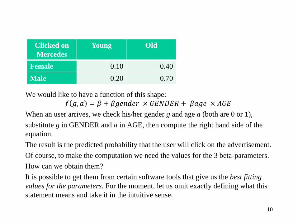
We would like to have a function of this shape:

𝑓 𝑔, 𝑎 = 𝛽 + 𝛽𝑔𝑒𝑛𝑑𝑒𝑟 × 𝐺𝐸𝑁𝐷𝐸𝑅 + 𝛽𝑎𝑔𝑒 × 𝐴𝐺𝐸

When an user arrives, we check his/her gender g and age a (both are 0 or 1),

substitute g in GENDER and a in AGE, then compute the right hand side of the

equation.

The result is the predicted probability that the user will click on the advertisement.

Of course, to make the computation we need the values for the 3 beta-parameters.

How can we obtain them?

It is possible to get them from certain software tools that give us the best fitting

values for the parameters. For the moment, let us omit exactly defining what this

statement means and take it in the intuitive sense.

Clicked on

Mercedes

Young Old

Female 0.10 0.40

Male 0.20 0.70

11

𝑓 𝑔, 𝑎 = 𝛽 + 𝛽𝑔𝑒𝑛𝑑𝑒𝑟 × 𝐺𝐸𝑁𝐷𝐸𝑅 + 𝛽𝑎𝑔𝑒 × 𝐴𝐺𝐸

An user arrives. We check it is a female of age classified as young (e.g., she is 24

and we classify as young any person below 30).

The user's attributes are GENDER = 1 and AGE = 1.

The parameters received by a tool are 𝛽 = 0.02, 𝛽𝑔𝑒𝑛𝑑𝑒𝑟 = 0.01, 𝛽𝑎𝑔𝑒 = 0.08

Substituting

𝑓 𝑔, 𝑎 = 0.02 + 0.01 × 1 + 0.08 × 1 = 0.11

The prediction is that the user will click with probability 11%.

Clicked on

Mercedes

Young Old

Female 0.10 0.40

Male 0.20 0.70

12

𝑓 𝑔, 𝑎 = 𝛽 + 𝛽𝑔𝑒𝑛𝑑𝑒𝑟 × 𝐺𝐸𝑁𝐷𝐸𝑅 + 𝛽𝑎𝑔𝑒 × 𝐴𝐺𝐸

Why doing such a complex procedure instead of simply getting the obvious

answer 10%? Data itself says that very clearly …

Yes, but available data is a sample out of the «true» population. Often it is too

small to be enough reliable. Often it is simply missing. If we have a lot of

attributes, often each combination of attribute values is seldom or never

represented in the dataset.

We adopt a different approach: using data to discover the impact of the attributes

on the answer (to click or not to click), then using attributes’ estimated impacts to

re-build an estimate of the answer.

So doing, estimates will be not equal to observed frequencies.

Clicked on

Mercedes

Young Old

Female 0.10 0.40

Male 0.20 0.70

13

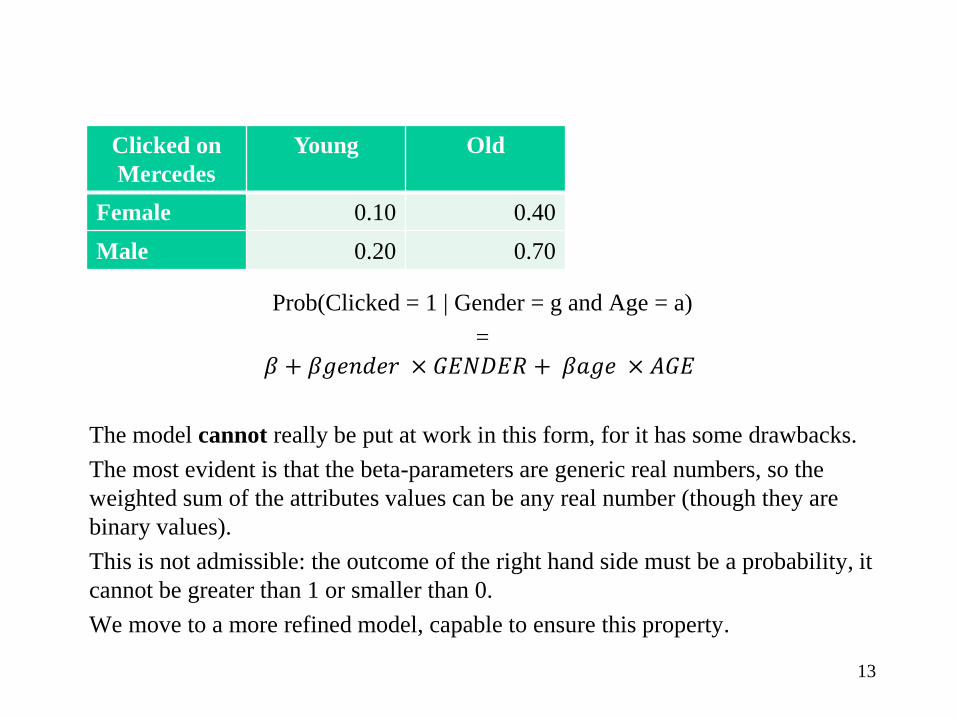
Prob(Clicked = 1 | Gender = g and Age = a)

=

𝛽 + 𝛽𝑔𝑒𝑛𝑑𝑒𝑟 × 𝐺𝐸𝑁𝐷𝐸𝑅 + 𝛽𝑎𝑔𝑒 × 𝐴𝐺𝐸

The model cannot really be put at work in this form, for it has some drawbacks.

The most evident is that the beta-parameters are generic real numbers, so the

weighted sum of the attributes values can be any real number (though they are

binary values).

This is not admissible: the outcome of the right hand side must be a probability, it

cannot be greater than 1 or smaller than 0.

We move to a more refined model, capable to ensure this property.

Clicked on

Mercedes

Young Old

Female 0.10 0.40

Male 0.20 0.70

14

Let

p = Prob(Clicked = 1 | Gender = g and Age = a),

logit(p) = log [p / (1 – p],

The new model is

logit(p) = 𝛽 + 𝛽𝑔𝑒𝑛𝑑𝑒𝑟 × 𝐺𝐸𝑁𝐷𝐸𝑅 + 𝛽𝑎𝑔𝑒 × 𝐴𝐺𝐸

that is, you substitute user attributes and parameters suggested by a Logistic

Regression tool and you get not exactly the predicted probability p, but its logit.

This is not a problem: once you know the logit(p), you can easily find p itself.

Clicked on

Mercedes

Young Old

Female 0.10 0.40

Male 0.20 0.70

Logistic regression model

15

p = Prob(Clicked = 1 | Gender = g and Age = a),

logit(p) = log(odds),

odds = p / (1 – p)

logit(p) = 𝛽 + 𝛽𝑔𝑒𝑛𝑑𝑒𝑟 × 𝐺𝐸𝑁𝐷𝐸𝑅 + 𝛽𝑎𝑔𝑒 × 𝐴𝐺𝐸

Odds are another view of probabilities.

In a bet where the probability of winning is p = 0.5 it is odds = 1. This is the fair

pot you have to gamble against a pot of 1. I.e., the bet is even and it you fairly bet

1€ vs. 1€.

If it is p = 0.75 then the odds are 3: you bet 3€ vs. 1€, if the bet is fair.

In logistic regression, the weighted sum of attributes gives the logarithm of the

odds.

Clicked on

Mercedes

Young Old

Female 0.10 0.40

Male 0.20 0.70

Odds

16

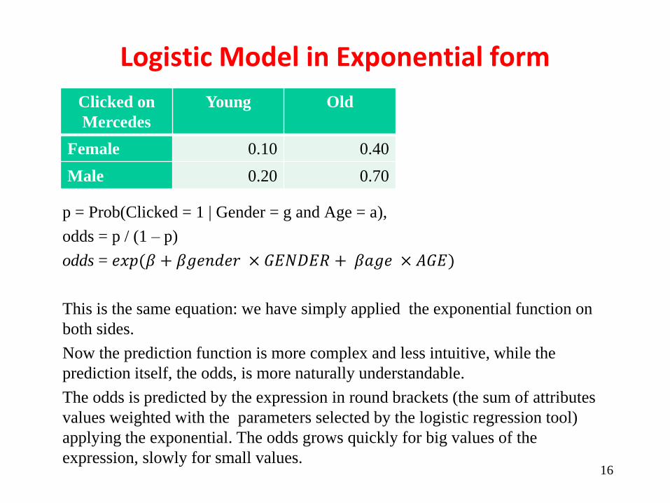
p = Prob(Clicked = 1 | Gender = g and Age = a),

odds = p / (1 – p)

odds = 𝑒𝑥𝑝(𝛽 + 𝛽𝑔𝑒𝑛𝑑𝑒𝑟 × 𝐺𝐸𝑁𝐷𝐸𝑅 + 𝛽𝑎𝑔𝑒 × 𝐴𝐺𝐸)

This is the same equation: we have simply applied the exponential function on

both sides.

Now the prediction function is more complex and less intuitive, while the

prediction itself, the odds, is more naturally understandable.

The odds is predicted by the expression in round brackets (the sum of attributes

values weighted with the parameters selected by the logistic regression tool)

applying the exponential. The odds grows quickly for big values of the

expression, slowly for small values.

Clicked on

Mercedes

Young Old

Female 0.10 0.40

Male 0.20 0.70

Logistic Model in Exponential form

17

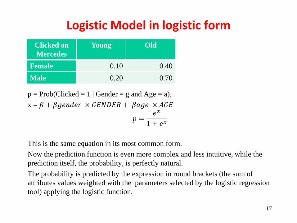
p = Prob(Clicked = 1 | Gender = g and Age = a),

x = 𝛽 + 𝛽𝑔𝑒𝑛𝑑𝑒𝑟 × 𝐺𝐸𝑁𝐷𝐸𝑅 + 𝛽𝑎𝑔𝑒 × 𝐴𝐺𝐸

𝑝 =𝑒𝑥

1 + 𝑒𝑥

This is the same equation in its most common form.

Now the prediction function is even more complex and less intuitive, while the

prediction itself, the probability, is perfectly natural.

The probability is predicted by the expression in round brackets (the sum of

attributes values weighted with the parameters selected by the logistic regression

tool) applying the logistic function.

Clicked on

Mercedes

Young Old

Female 0.10 0.40

Male 0.20 0.70

Logistic Model in logistic form