Logistic Regression - Cleveland State University

Page 1 of 11

Itza Perez

Logistic Regression

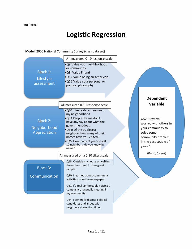
I. Model: 2006 National Community Survey (class data set)

•Q9:Value your neighborhood or community

•Q8: Value Friend

•Q12:Value being an American

•Q15:Value your personal or political philosophy

Block 1:

Lifestyle assessment

•Q30: I feel safe and secure in my neighborhood

•Q33:People like me don't have any say about what the government does.

•Q34: Of the 10 closest neighbors,how many of their homes have you visited?

•Q35: How many of your closest 10 neighbors do you know by name?

Block 2:

Neighborhood Appreciation

Block 3:

Communication

Q18: Outside my house or walking down the street, I often greet people.

Q20: I learned about community activities from the newspaper.

Q21: I’d feel comfortable voicing a complaint at a public meeting in my community.

Q24: I generally discuss political candidates and issues with neighbors at election time.

Dependent

Variable

Q52: Have you

worked with others in

your community to

solve some

community problem

in the past couple of

years?

(0=no, 1=yes)

All measured 0-10 response scale

All measured 0-10 response scale

All measured on a 0-10 Likert scale

Page 2 of 11

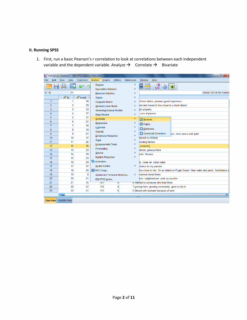
II. Running SPSS

1. First, run a basic Pearson’s r correlation to look at correlations between each independent

variable and the dependent variable. Analyze Correlate Bivariate

Page 3 of 11

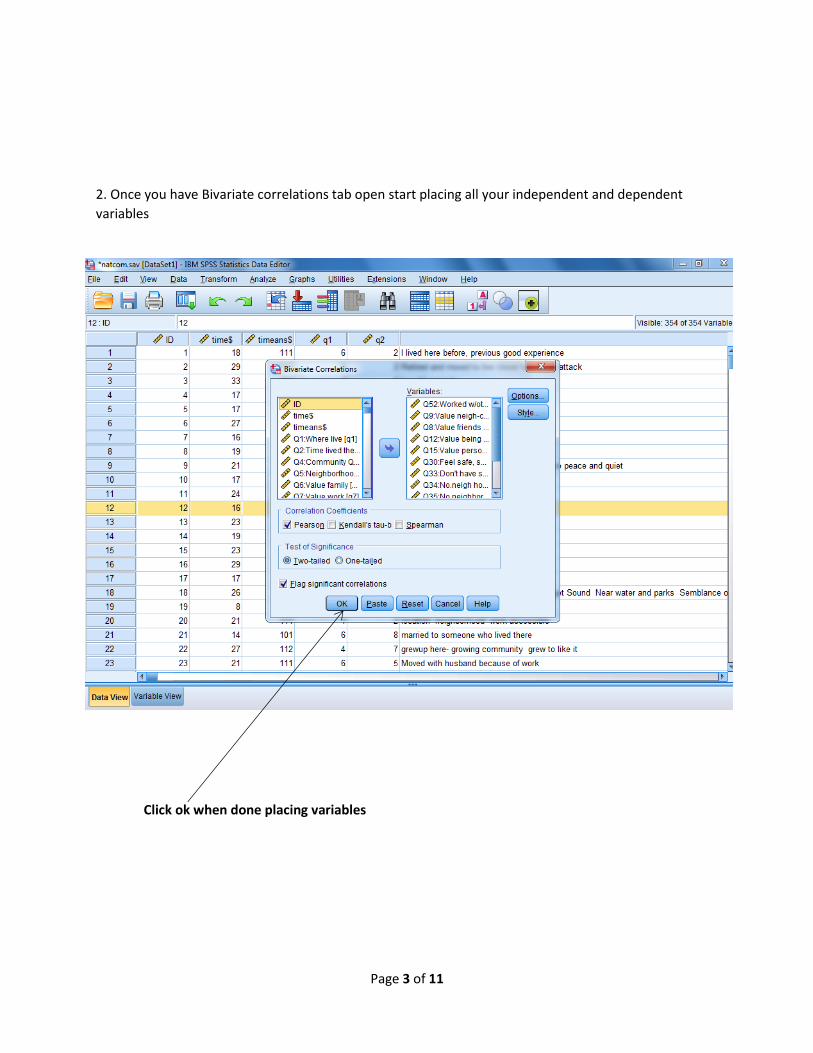
2. Once you have Bivariate correlations tab open start placing all your independent and dependent

variables

Click ok when done placing variables

Page 4 of 11

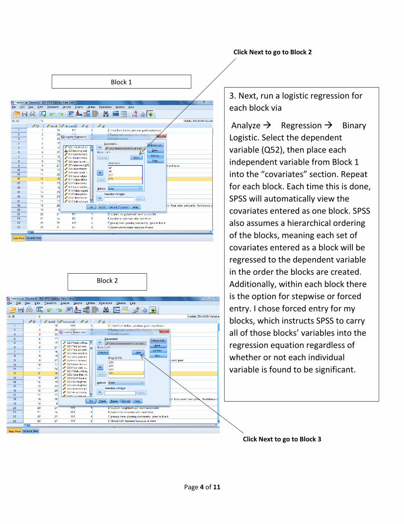
Click Next to go to Block 2

Click Next to go to Block 3

Block 1

Block 2

3. Next, run a logistic regression for

each block via

Analyze Regression Binary

Logistic. Select the dependent

variable (Q52), then place each

independent variable from Block 1

into the “covariates” section. Repeat

for each block. Each time this is done,

SPSS will automatically view the

covariates entered as one block. SPSS

also assumes a hierarchical ordering

of the blocks, meaning each set of

covariates entered as a block will be

regressed to the dependent variable

in the order the blocks are created.

Additionally, within each block there

is the option for stepwise or forced

entry. I chose forced entry for my

blocks, which instructs SPSS to carry

all of those blocks’ variables into the

regression equation regardless of

whether or not each individual

variable is found to be significant.

Page 5 of 11

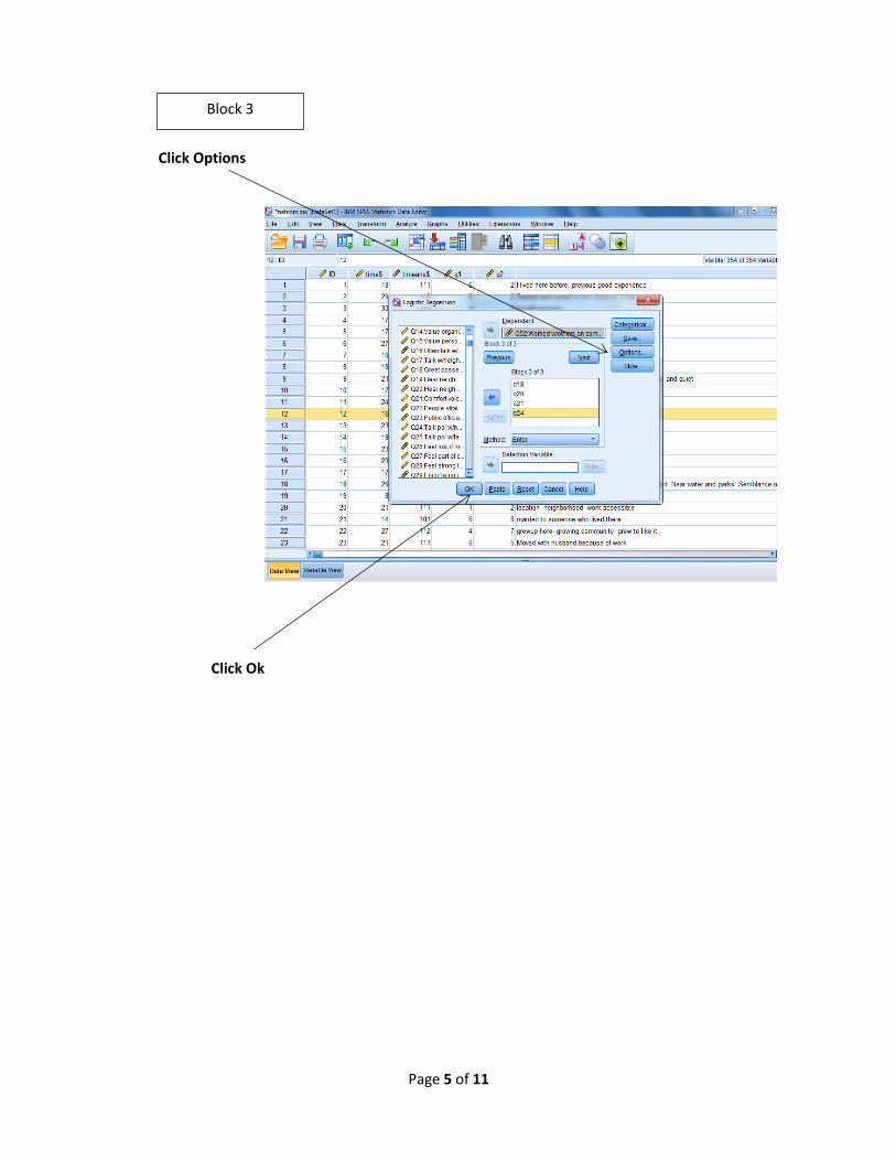
Click Options

Click Ok

Block 3

Page 6 of 11

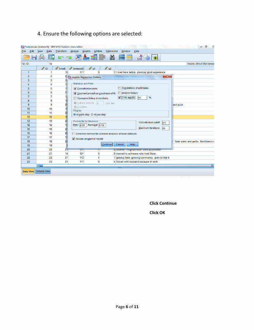
4. Ensure the following options are selected:

Click Continue

Click OK

Page 7 of 11

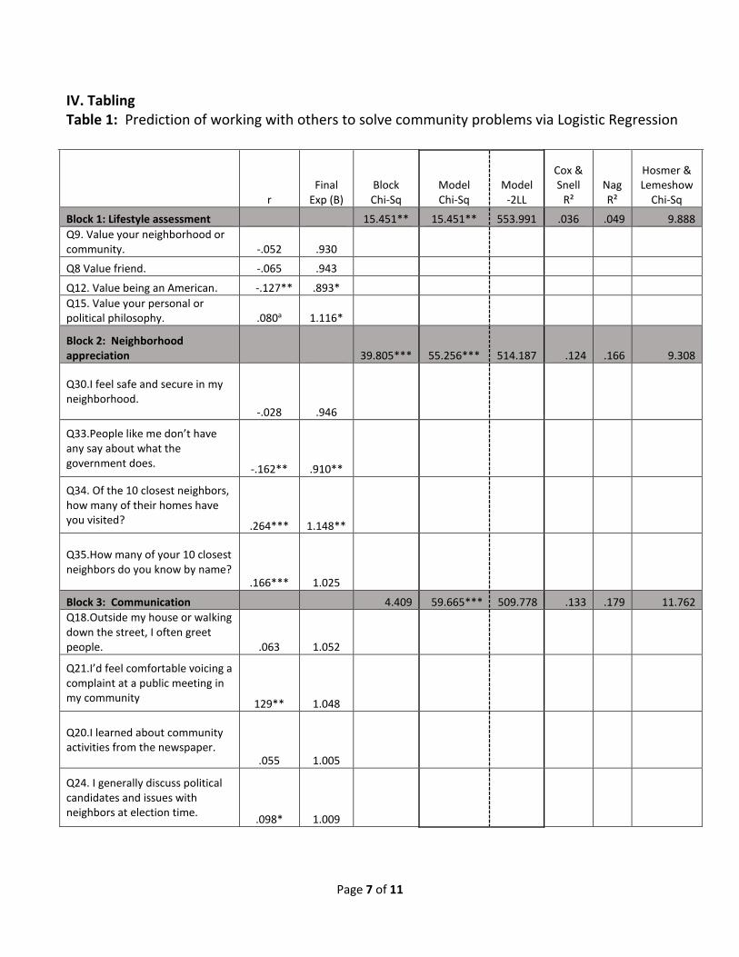
IV. Tabling Table 1: Prediction of working with others to solve community problems via Logistic Regression

r Final

Exp (B) Block Chi-Sq

Model Chi-Sq

Model -2LL

Cox & Snell

R² Nag R²

Hosmer & Lemeshow

Chi-Sq

Block 1: Lifestyle assessment 15.451** 15.451** 553.991 .036 .049 9.888

Q9. Value your neighborhood or community. -.052 .930

Q8 Value friend. -.065 .943

Q12. Value being an American. -.127** .893*

Q15. Value your personal or political philosophy. .080a 1.116*

Block 2: Neighborhood appreciation 39.805*** 55.256*** 514.187 .124 .166 9.308

Q30.I feel safe and secure in my neighborhood.

-.028 .946

Q33.People like me don’t have any say about what the government does. -.162** .910**

Q34. Of the 10 closest neighbors, how many of their homes have you visited?

.264*** 1.148**

Q35.How many of your 10 closest neighbors do you know by name?

.166*** 1.025

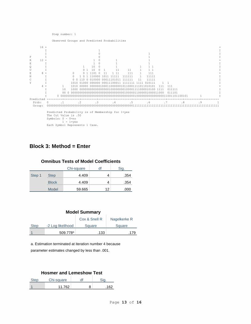
Block 3: Communication 4.409 59.665*** 509.778 .133 .179 11.762

Q18.Outside my house or walking down the street, I often greet people. .063 1.052

Q21.I’d feel comfortable voicing a complaint at a public meeting in my community

129** 1.048

Q20.I learned about community activities from the newspaper.

.055 1.005

Q24. I generally discuss political candidates and issues with neighbors at election time.

.098* 1.009

Page 8 of 11

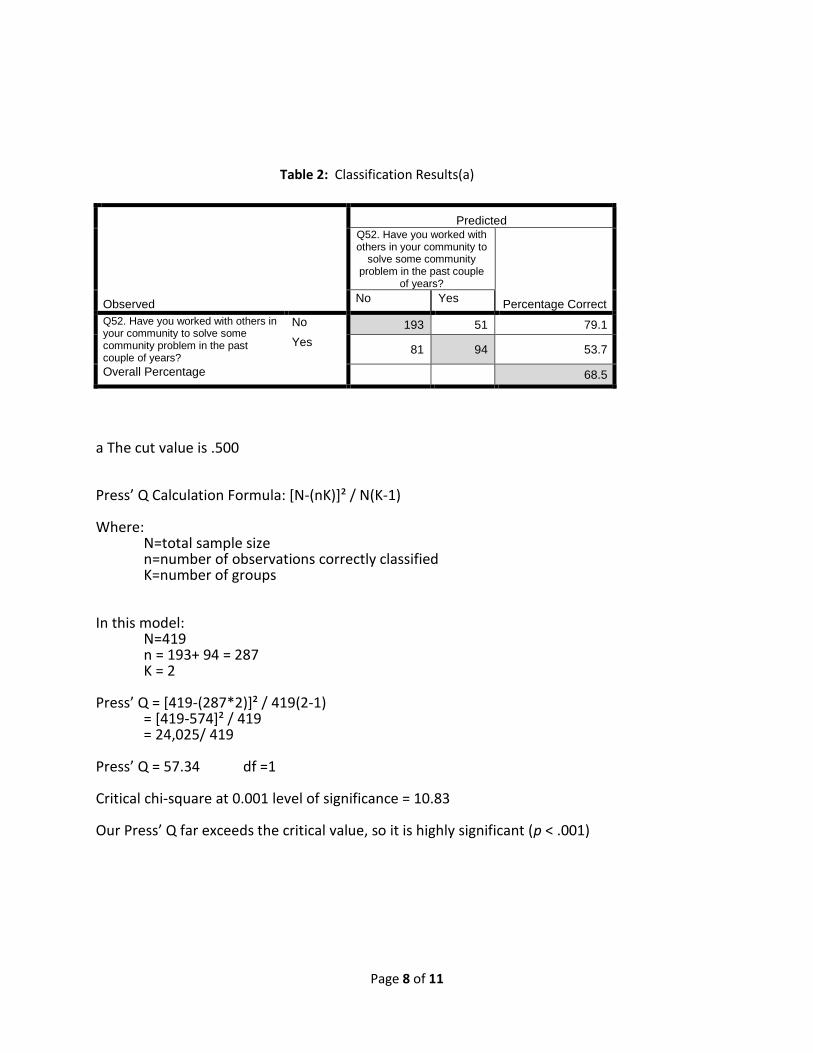
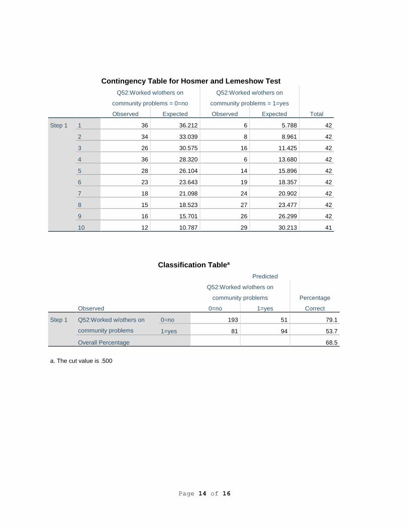
Table 2: Classification Results(a)

Observed

Predicted Q52. Have you worked with others in your community to

solve some community problem in the past couple

of years?

Percentage Correct No Yes

Q52. Have you worked with others in your community to solve some community problem in the past couple of years?

No 193 51 79.1

Yes 81 94 53.7

Overall Percentage 68.5

a The cut value is .500

Press’ Q Calculation Formula: [N-(nK)]² / N(K-1) Where:

N=total sample size n=number of observations correctly classified K=number of groups

In this model: N=419 n = 193+ 94 = 287 K = 2

Press’ Q = [419-(287*2)]² / 419(2-1) = [419-574]² / 419 = 24,025/ 419

Press’ Q = 57.34 df =1 Critical chi-square at 0.001 level of significance = 10.83 Our Press’ Q far exceeds the critical value, so it is highly significant (p < .001)

Page 9 of 11

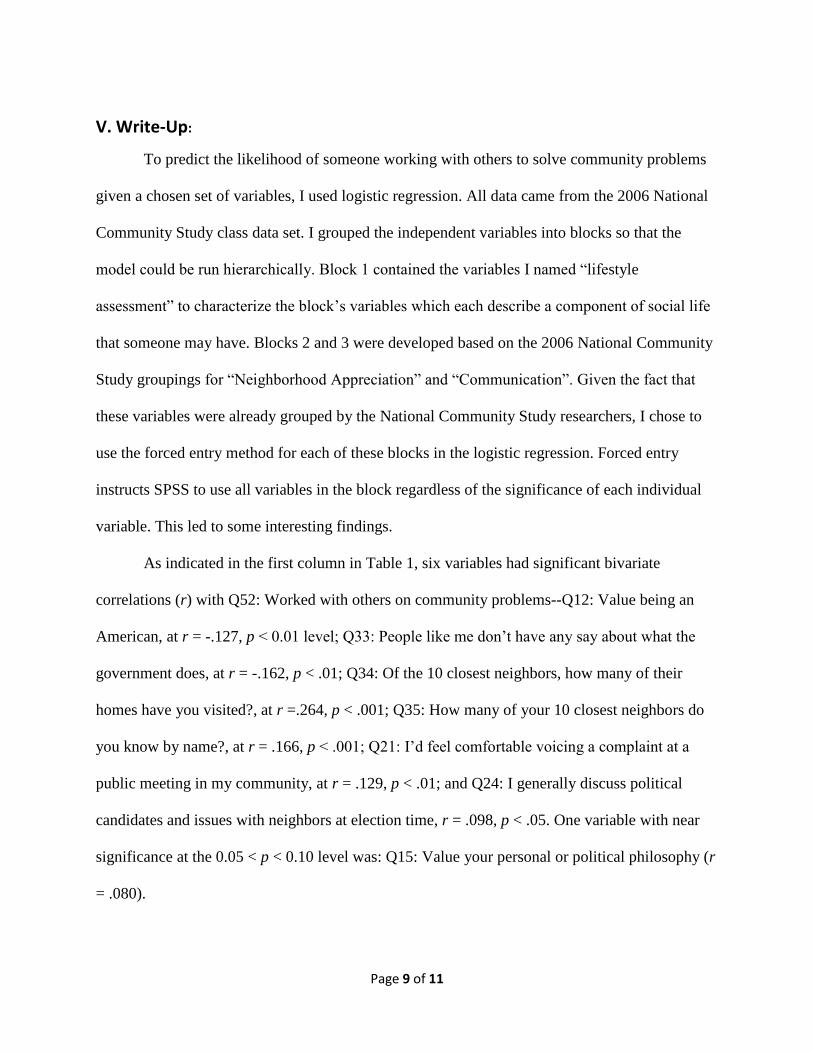
V. Write-Up:

To predict the likelihood of someone working with others to solve community problems

given a chosen set of variables, I used logistic regression. All data came from the 2006 National

Community Study class data set. I grouped the independent variables into blocks so that the

model could be run hierarchically. Block 1 contained the variables I named “lifestyle

assessment” to characterize the block’s variables which each describe a component of social life

that someone may have. Blocks 2 and 3 were developed based on the 2006 National Community

Study groupings for “Neighborhood Appreciation” and “Communication”. Given the fact that

these variables were already grouped by the National Community Study researchers, I chose to

use the forced entry method for each of these blocks in the logistic regression. Forced entry

instructs SPSS to use all variables in the block regardless of the significance of each individual

variable. This led to some interesting findings.

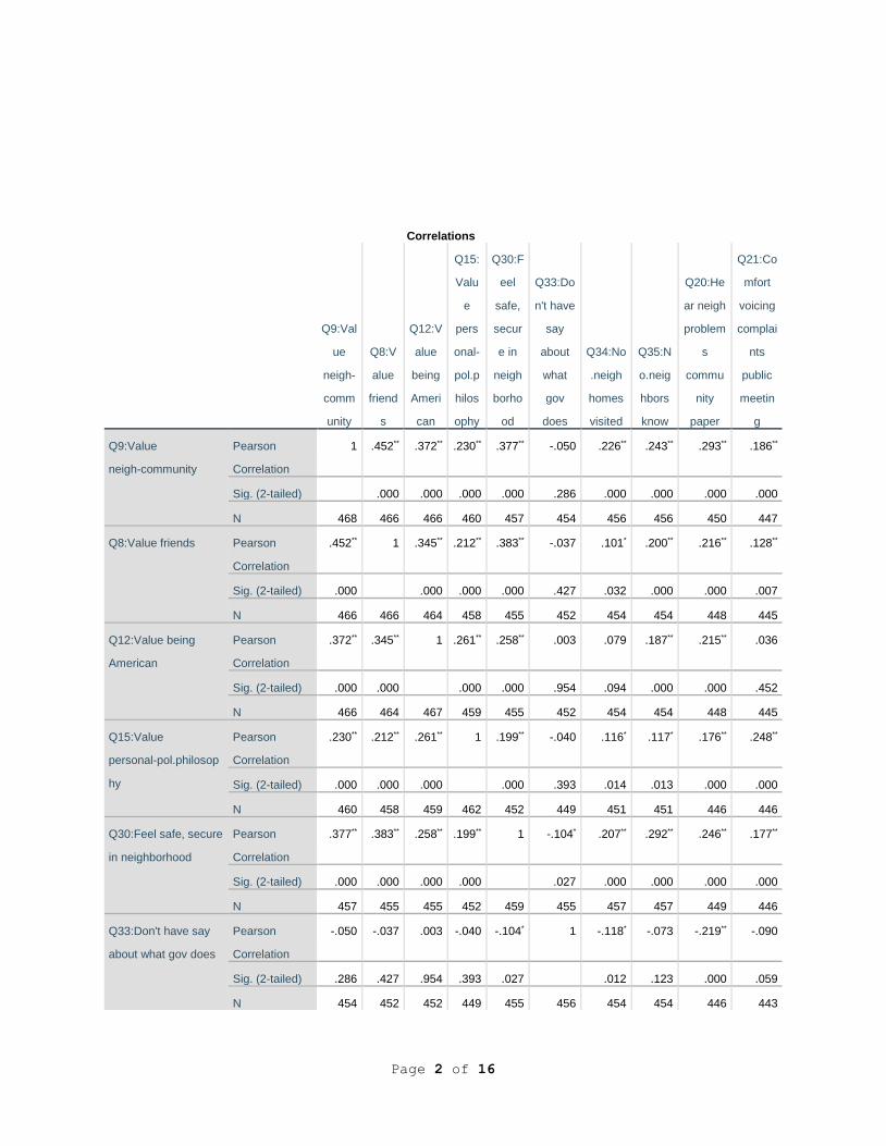
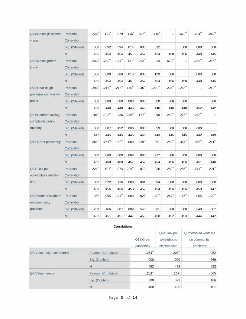
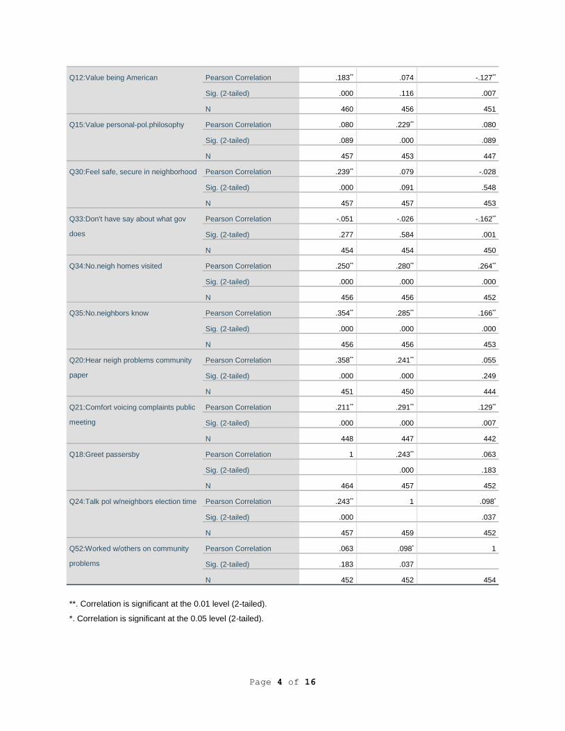
As indicated in the first column in Table 1, six variables had significant bivariate

correlations (r) with Q52: Worked with others on community problems--Q12: Value being an

American, at r = -.127, p < 0.01 level; Q33: People like me don’t have any say about what the

government does, at r = -.162, p < .01; Q34: Of the 10 closest neighbors, how many of their

homes have you visited?, at r =.264, p < .001; Q35: How many of your 10 closest neighbors do

you know by name?, at r = .166, p < .001; Q21: I’d feel comfortable voicing a complaint at a

public meeting in my community, at r = .129, p < .01; and Q24: I generally discuss political

candidates and issues with neighbors at election time, r = .098, p < .05. One variable with near

significance at the 0.05 < p < 0.10 level was: Q15: Value your personal or political philosophy (r

= .080).

Page 10 of 11

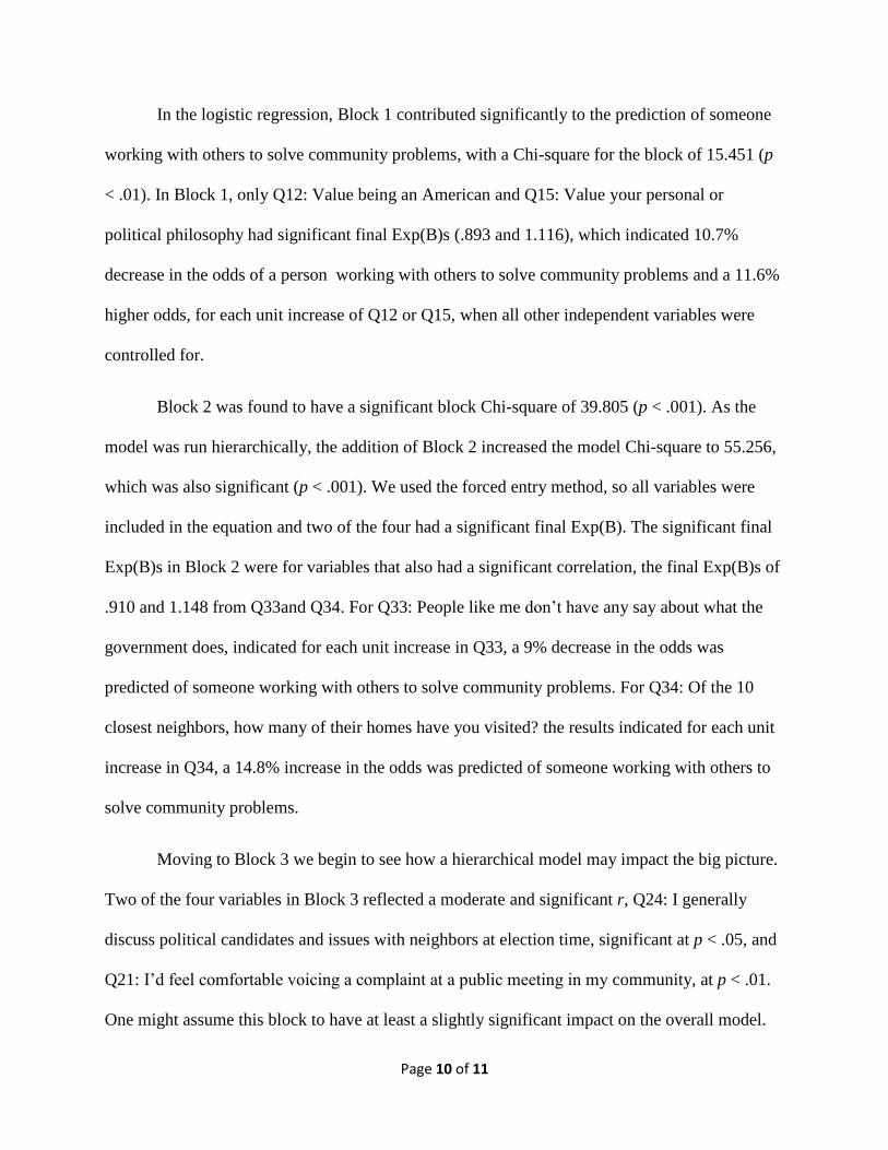
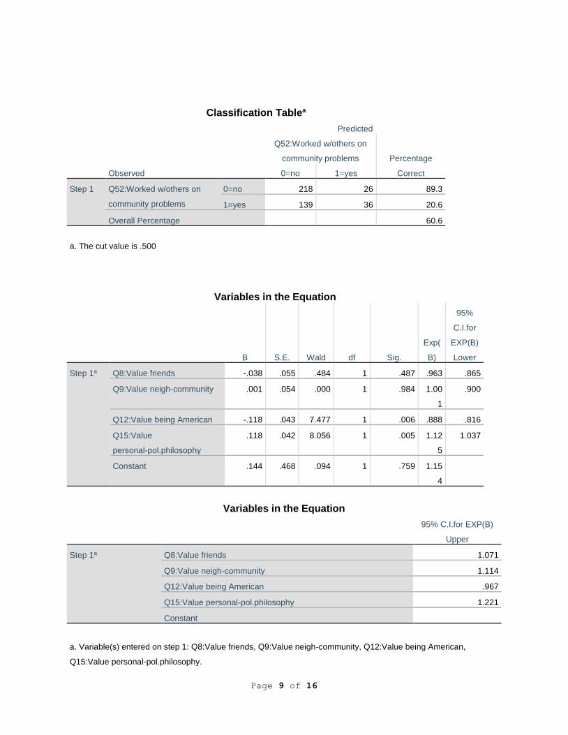
In the logistic regression, Block 1 contributed significantly to the prediction of someone

working with others to solve community problems, with a Chi-square for the block of 15.451 (p

< .01). In Block 1, only Q12: Value being an American and Q15: Value your personal or

political philosophy had significant final Exp(B)s (.893 and 1.116), which indicated 10.7%

decrease in the odds of a person working with others to solve community problems and a 11.6%

higher odds, for each unit increase of Q12 or Q15, when all other independent variables were

controlled for.

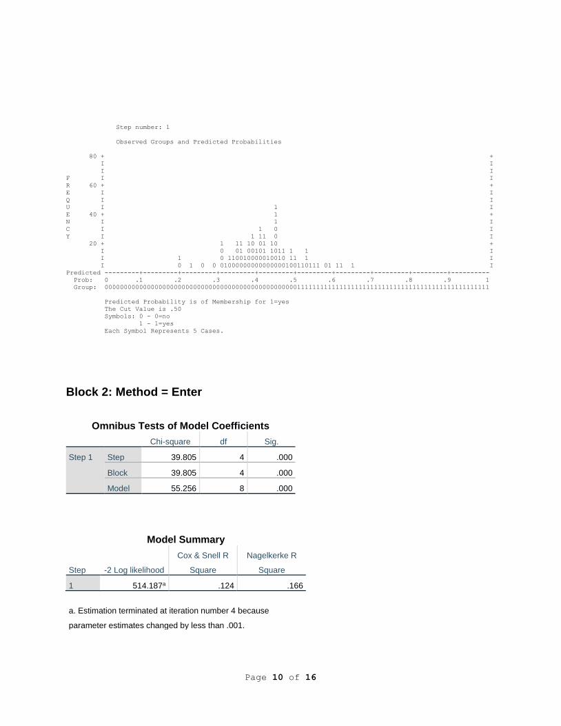
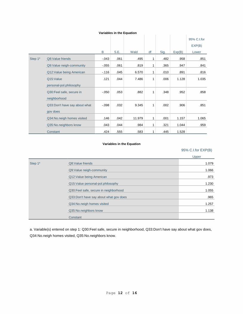
Block 2 was found to have a significant block Chi-square of 39.805 (p < .001). As the

model was run hierarchically, the addition of Block 2 increased the model Chi-square to 55.256,

which was also significant (p < .001). We used the forced entry method, so all variables were

included in the equation and two of the four had a significant final Exp(B). The significant final

Exp(B)s in Block 2 were for variables that also had a significant correlation, the final Exp(B)s of

.910 and 1.148 from Q33and Q34. For Q33: People like me don’t have any say about what the

government does, indicated for each unit increase in Q33, a 9% decrease in the odds was

predicted of someone working with others to solve community problems. For Q34: Of the 10

closest neighbors, how many of their homes have you visited? the results indicated for each unit

increase in Q34, a 14.8% increase in the odds was predicted of someone working with others to

solve community problems.

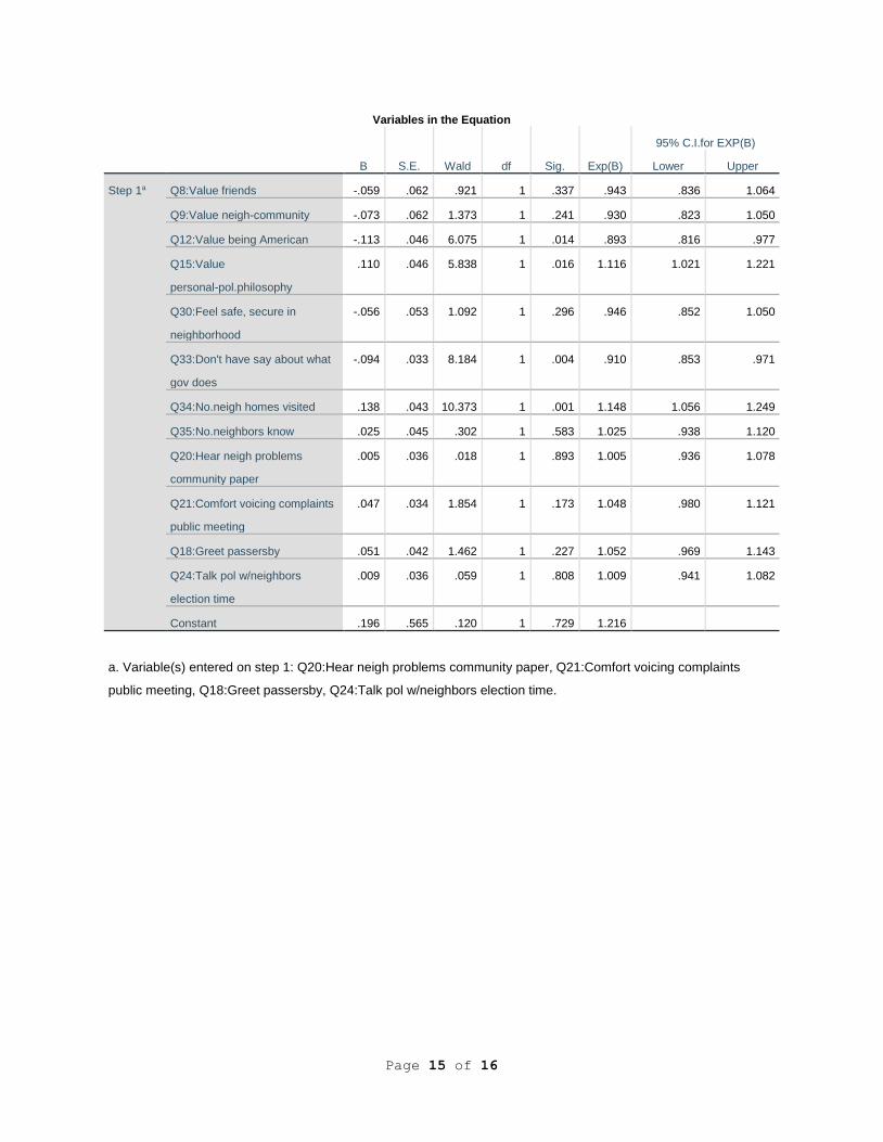
Moving to Block 3 we begin to see how a hierarchical model may impact the big picture.

Two of the four variables in Block 3 reflected a moderate and significant r, Q24: I generally

discuss political candidates and issues with neighbors at election time, significant at p < .05, and

Q21: I’d feel comfortable voicing a complaint at a public meeting in my community, at p < .01.

One might assume this block to have at least a slightly significant impact on the overall model.

Page 11 of 11

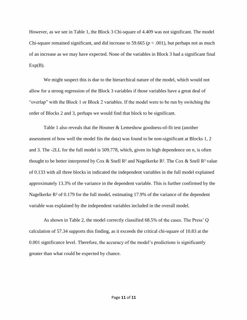
However, as we see in Table 1, the Block 3 Chi-square of 4.409 was not significant. The model

Chi-square remained significant, and did increase to 59.665 (p < .001), but perhaps not as much

of an increase as we may have expected. None of the variables in Block 3 had a significant final

Exp(B).

We might suspect this is due to the hierarchical nature of the model, which would not

allow for a strong regression of the Block 3 variables if those variables have a great deal of

“overlap” with the Block 1 or Block 2 variables. If the model were to be run by switching the

order of Blocks 2 and 3, perhaps we would find that block to be significant.

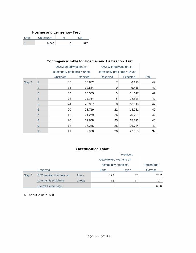
Table 1 also reveals that the Hosmer & Lemeshow goodness-of-fit test (another

assessment of how well the model fits the data) was found to be non-significant at Blocks 1, 2

and 3. The -2LL for the full model is 509.778, which, given its high dependence on n, is often

thought to be better interpreted by Cox & Snell R² and Nagelkerke R². The Cox & Snell R² value

of 0.133 with all three blocks in indicated the independent variables in the full model explained

approximately 13.3% of the variance in the dependent variable. This is further confirmed by the

Nagelkerke R² of 0.179 for the full model, estimating 17.9% of the variance of the dependent

variable was explained by the independent variables included in the overall model.

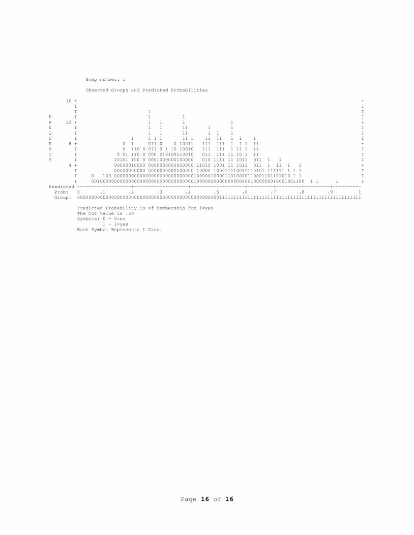
As shown in Table 2, the model correctly classified 68.5% of the cases. The Press’ Q

calculation of 57.34 supports this finding, as it exceeds the critical chi-square of 10.83 at the

0.001 significance level. Therefore, the accuracy of the model’s predictions is significantly

greater than what could be expected by chance.

Page 1 of 16

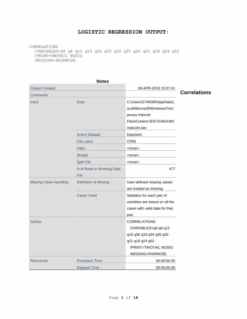
LOGISTIC REGRESSION OUTPUT:

CORRELATIONS

/VARIABLES=q9 q8 q12 q15 q30 q33 q34 q35 q20 q21 q18 q24 q52

/PRINT=TWOTAIL NOSIG

/MISSING=PAIRWISE.

Correlations

Notes

Output Created 08-APR-2019 15:37:41

Comments

Input Data C:\Users\2740585\AppData\L

ocal\Microsoft\Windows\Tem

porary Internet

Files\Content.IE5\7G46VH9X

\natcom.sav

Active Dataset DataSet1

File Label CP05

Filter <none>

Weight <none>

Split File <none>

N of Rows in Working Data

File

477

Missing Value Handling Definition of Missing User-defined missing values

are treated as missing.

Cases Used Statistics for each pair of

variables are based on all the

cases with valid data for that

pair.

Syntax CORRELATIONS

/VARIABLES=q9 q8 q12

q15 q30 q33 q34 q35 q20

q21 q18 q24 q52

/PRINT=TWOTAIL NOSIG

/MISSING=PAIRWISE.

Resources Processor Time 00:00:00.05

Elapsed Time 00:00:00.06

Page 2 of 16

Correlations

Q9:Val

ue

neigh-

comm

unity

Q8:V

alue

friend

s

Q12:V

alue

being

Ameri

can

Q15:

Valu

e

pers

onal-

pol.p

hilos

ophy

Q30:F

eel

safe,

secur

e in

neigh

borho

od

Q33:Do

n't have

say

about

what

gov

does

Q34:No

.neigh

homes

visited

Q35:N

o.neig

hbors

know

Q20:He

ar neigh

problem

s

commu

nity

paper

Q21:Co

mfort

voicing

complai

nts

public

meetin

g

Q9:Value

neigh-community

Pearson

Correlation

1 .452** .372** .230** .377** -.050 .226** .243** .293** .186**

Sig. (2-tailed) .000 .000 .000 .000 .286 .000 .000 .000 .000

N 468 466 466 460 457 454 456 456 450 447

Q8:Value friends Pearson

Correlation

.452** 1 .345** .212** .383** -.037 .101* .200** .216** .128**

Sig. (2-tailed) .000 .000 .000 .000 .427 .032 .000 .000 .007

N 466 466 464 458 455 452 454 454 448 445

Q12:Value being

American

Pearson

Correlation

.372** .345** 1 .261** .258** .003 .079 .187** .215** .036

Sig. (2-tailed) .000 .000 .000 .000 .954 .094 .000 .000 .452

N 466 464 467 459 455 452 454 454 448 445

Q15:Value

personal-pol.philosop

hy

Pearson

Correlation

.230** .212** .261** 1 .199** -.040 .116* .117* .176** .248**

Sig. (2-tailed) .000 .000 .000 .000 .393 .014 .013 .000 .000

N 460 458 459 462 452 449 451 451 446 446

Q30:Feel safe, secure

in neighborhood

Pearson

Correlation

.377** .383** .258** .199** 1 -.104* .207** .292** .246** .177**

Sig. (2-tailed) .000 .000 .000 .000 .027 .000 .000 .000 .000

N 457 455 455 452 459 455 457 457 449 446

Q33:Don't have say

about what gov does

Pearson

Correlation

-.050 -.037 .003 -.040 -.104* 1 -.118* -.073 -.219** -.090

Sig. (2-tailed) .286 .427 .954 .393 .027 .012 .123 .000 .059

N 454 452 452 449 455 456 454 454 446 443

Page 3 of 16

Q34:No.neigh homes

visited

Pearson

Correlation

.226** .101* .079 .116* .207** -.118* 1 .612** .224** .242**

Sig. (2-tailed) .000 .032 .094 .014 .000 .012 .000 .000 .000

N 456 454 454 451 457 454 458 456 448 445

Q35:No.neighbors

know

Pearson

Correlation

.243** .200** .187** .117* .292** -.073 .612** 1 .266** .215**

Sig. (2-tailed) .000 .000 .000 .013 .000 .123 .000 .000 .000

N 456 454 454 451 457 454 456 458 448 445

Q20:Hear neigh

problems community

paper

Pearson

Correlation

.293** .216** .215** .176** .246** -.219** .224** .266** 1 .242**

Sig. (2-tailed) .000 .000 .000 .000 .000 .000 .000 .000 .000

N 450 448 448 446 449 446 448 448 452 442

Q21:Comfort voicing

complaints public

meeting

Pearson

Correlation

.186** .128** .036 .248** .177** -.090 .242** .215** .242** 1

Sig. (2-tailed) .000 .007 .452 .000 .000 .059 .000 .000 .000

N 447 445 445 446 446 443 445 445 442 449

Q18:Greet passersby Pearson

Correlation

.261** .251** .183** .080 .239** -.051 .250** .354** .358** .211**

Sig. (2-tailed) .000 .000 .000 .089 .000 .277 .000 .000 .000 .000

N 462 460 460 457 457 454 456 456 451 448

Q24:Talk pol

w/neighbors election

time

Pearson

Correlation

.221** .107* .074 .229** .079 -.026 .280** .285** .241** .291**

Sig. (2-tailed) .000 .022 .116 .000 .091 .584 .000 .000 .000 .000

N 458 456 456 453 457 454 456 456 450 447

Q52:Worked w/others

on community

problems

Pearson

Correlation

-.052 -.065 -.127** .080 -.028 -.162** .264** .166** .055 .129**

Sig. (2-tailed) .269 .166 .007 .089 .548 .001 .000 .000 .249 .007

N 453 451 451 447 453 450 452 453 444 442

Correlations

Q18:Greet

passersby

Q24:Talk pol

w/neighbors

election time

Q52:Worked w/others

on community

problems

Q9:Value neigh-community Pearson Correlation .261** .221** -.052

Sig. (2-tailed) .000 .000 .269

N 462 458 453

Q8:Value friends Pearson Correlation .251** .107* -.065

Sig. (2-tailed) .000 .022 .166

N 460 456 451

Page 4 of 16

Q12:Value being American Pearson Correlation .183** .074 -.127**

Sig. (2-tailed) .000 .116 .007

N 460 456 451

Q15:Value personal-pol.philosophy Pearson Correlation .080 .229** .080

Sig. (2-tailed) .089 .000 .089

N 457 453 447

Q30:Feel safe, secure in neighborhood Pearson Correlation .239** .079 -.028

Sig. (2-tailed) .000 .091 .548

N 457 457 453

Q33:Don't have say about what gov

does

Pearson Correlation -.051 -.026 -.162**

Sig. (2-tailed) .277 .584 .001

N 454 454 450

Q34:No.neigh homes visited Pearson Correlation .250** .280** .264**

Sig. (2-tailed) .000 .000 .000

N 456 456 452

Q35:No.neighbors know Pearson Correlation .354** .285** .166**

Sig. (2-tailed) .000 .000 .000

N 456 456 453

Q20:Hear neigh problems community

paper

Pearson Correlation .358** .241** .055

Sig. (2-tailed) .000 .000 .249

N 451 450 444

Q21:Comfort voicing complaints public

meeting

Pearson Correlation .211** .291** .129**

Sig. (2-tailed) .000 .000 .007

N 448 447 442

Q18:Greet passersby Pearson Correlation 1 .243** .063

Sig. (2-tailed) .000 .183

N 464 457 452

Q24:Talk pol w/neighbors election time Pearson Correlation .243** 1 .098*

Sig. (2-tailed) .000 .037

N 457 459 452

Q52:Worked w/others on community

problems

Pearson Correlation .063 .098* 1

Sig. (2-tailed) .183 .037

N 452 452 454

**. Correlation is significant at the 0.01 level (2-tailed).

*. Correlation is significant at the 0.05 level (2-tailed).

Page 5 of 16

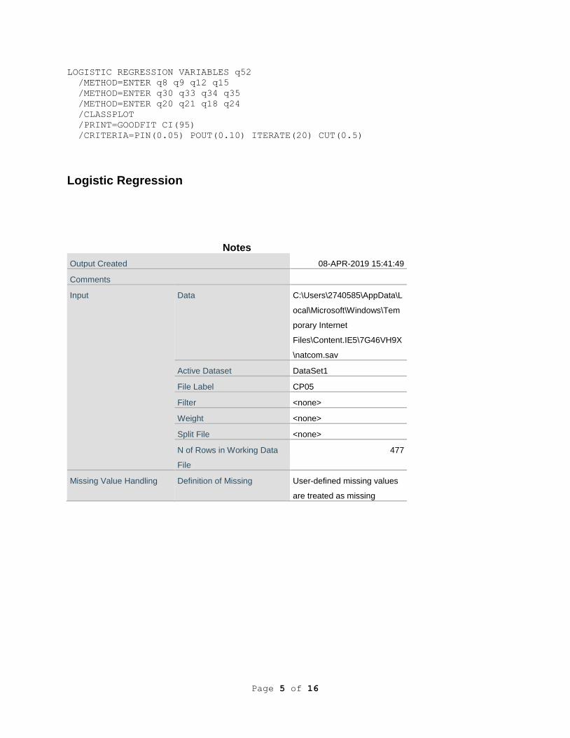
LOGISTIC REGRESSION VARIABLES q52

/METHOD=ENTER q8 q9 q12 q15



/CLASSPLOT

/PRINT=GOODFIT CI(95)

/CRITERIA=PIN(0.05) POUT(0.10) ITERATE(20) CUT(0.5)

Logistic Regression

Notes

Output Created 08-APR-2019 15:41:49

Comments

Input Data C:\Users\2740585\AppData\L

ocal\Microsoft\Windows\Tem

porary Internet

Files\Content.IE5\7G46VH9X

\natcom.sav

Active Dataset DataSet1

File Label CP05

Filter <none>

Weight <none>

Split File <none>

N of Rows in Working Data

File

477

Missing Value Handling Definition of Missing User-defined missing values

are treated as missing

Page 6 of 16

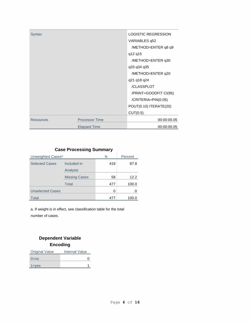
Syntax LOGISTIC REGRESSION

VARIABLES q52

/METHOD=ENTER q8 q9

q12 q15

/METHOD=ENTER q30

q33 q34 q35

/METHOD=ENTER q20

q21 q18 q24

/CLASSPLOT

/PRINT=GOODFIT CI(95)

/CRITERIA=PIN(0.05)

POUT(0.10) ITERATE(20)

CUT(0.5).

Resources Processor Time 00:00:00.05

Elapsed Time 00:00:00.05

Case Processing Summary

Unweighted Casesa N Percent

Selected Cases Included in

Analysis

419 87.8

Missing Cases 58 12.2

Total 477 100.0

Unselected Cases 0 .0

Total 477 100.0

a. If weight is in effect, see classification table for the total

number of cases.

Dependent Variable

Encoding

Original Value Internal Value

0=no 0

1=yes 1

Page 7 of 16

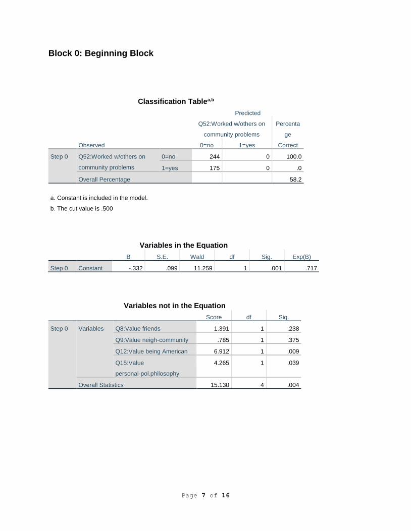
Block 0: Beginning Block

Classification Tablea,b

Observed

Predicted

Q52:Worked w/others on

community problems

Percenta

ge

Correct 0=no 1=yes

Step 0 Q52:Worked w/others on

community problems

0=no 244 0 100.0

1=yes 175 0 .0


a. Constant is included in the model.

b. The cut value is .500

Variables in the Equation

B S.E. Wald df Sig. Exp(B)

Step 0 Constant -.332 .099 11.259 1 .001 .717

Variables not in the Equation

Score df Sig.

Step 0 Variables Q8:Value friends 1.391 1 .238

Q9:Value neigh-community .785 1 .375

Q12:Value being American 6.912 1 .009

Q15:Value

personal-pol.philosophy

4.265 1 .039

Overall Statistics 15.130 4 .004

Page 8 of 16

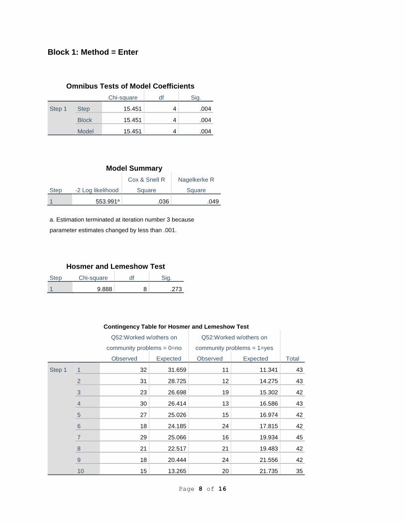
Block 1: Method = Enter

Omnibus Tests of Model Coefficients

Chi-square df Sig.

Step 1 Step 15.451 4 .004

Block 15.451 4 .004

Model 15.451 4 .004

Model Summary

Step -2 Log likelihood

Cox & Snell R

Square

Nagelkerke R

Square

1 553.991a .036 .049

a. Estimation terminated at iteration number 3 because

parameter estimates changed by less than .001.

Hosmer and Lemeshow Test

Step Chi-square df Sig.

1 9.888 8 .273

Contingency Table for Hosmer and Lemeshow Test


community problems = 0=no


community problems = 1=yes

Total Observed Expected Observed Expected

Step 1 1 32 31.659 11 11.341 43

2 31 28.725 12 14.275 43

3 23 26.698 19 15.302 42

4 30 26.414 13 16.586 43

5 27 25.026 15 16.974 42

6 18 24.185 24 17.815 42

7 29 25.066 16 19.934 45

8 21 22.517 21 19.483 42

9 18 20.444 24 21.556 42

10 15 13.265 20 21.735 35

Page 9 of 16

Classification Tablea

Observed

Predicted


community problems Percentage

Correct 0=no 1=yes


community problems

0=no 218 26 89.3

1=yes 139 36 20.6


a. The cut value is .500


B S.E. Wald df Sig.

Exp(

B)

95%

C.I.for

EXP(B)

Lower

Step 1a Q8:Value friends -.038 .055 .484 1 .487 .963 .865

Q9:Value neigh-community .001 .054 .000 1 .984 1.00

1

.900

Q12:Value being American -.118 .043 7.477 1 .006 .888 .816

Q15:Value


.118 .042 8.056 1 .005 1.12

5

1.037

Constant .144 .468 .094 1 .759 1.15

4


95% C.I.for EXP(B)

Upper

Step 1a Q8:Value friends 1.071

Q9:Value neigh-community 1.114

Q12:Value being American .967

Q15:Value personal-pol.philosophy 1.221

Constant

a. Variable(s) entered on step 1: Q8:Value friends, Q9:Value neigh-community, Q12:Value being American,

Q15:Value personal-pol.philosophy.

Page 10 of 16

Step number: 1

Observed Groups and Predicted Probabilities

80 + +

I I

I I

F I I

R 60 + +

E I I

Q I I

U I 1 I

E 40 + 1 +

N I 1 I

C I 1 0 I

Y I 1 11 0 I

20 + 1 11 10 01 10 +

I 0 01 00101 1011 1 1 I

I 1 0 110010000010010 11 1 I

I 0 1 0 0 01000000000000000100110111 01 11 1 I

Predicted ---------+---------+---------+---------+---------+---------+---------+---------+---------+----------

Prob: 0 .1 .2 .3 .4 .5 .6 .7 .8 .9 1

Group: 0000000000000000000000000000000000000000000000000011111111111111111111111111111111111111111111111111

Predicted Probability is of Membership for 1=yes

The Cut Value is .50

Symbols: 0 - 0=no

1 - 1=yes

Each Symbol Represents 5 Cases.



Chi-square df Sig.

Step 1 Step 39.805 4 .000

Block 39.805 4 .000

Model 55.256 8 .000

Model Summary


Cox & Snell R

Square

Nagelkerke R

Square

1 514.187a .124 .166



Page 11 of 16



1 9.308 8 .317







Step 1 1 35 35.882 7 6.118 42

2 33 32.584 9 9.416 42

3 33 30.353 9 11.647 42

4 34 28.364 8 13.636 42

5 24 25.987 18 16.013 42

6 20 23.719 22 18.281 42

7 16 21.279 26 20.721 42

8 20 19.608 25 25.392 45

9 18 16.256 25 26.744 43

10 11 9.970 26 27.030 37


Observed

Predicted



Correct 0=no 1=yes


community problems

0=no 192 52 78.7

1=yes 88 87 49.7



Page 12 of 16



95% C.I.for

EXP(B)

Lower

Step 1a Q8:Value friends -.043 .061 .495 1 .482 .958 .851

Q9:Value neigh-community -.055 .061 .819 1 .365 .947 .841

Q12:Value being American -.116 .045 6.570 1 .010 .891 .816

Q15:Value


.121 .044 7.486 1 .006 1.128 1.035

Q30:Feel safe, secure in

neighborhood

-.050 .053 .882 1 .348 .952 .858

Q33:Don't have say about what

gov does

-.098 .032 9.345 1 .002 .906 .851

Q34:No.neigh homes visited .146 .042 11.979 1 .001 1.157 1.065

Q35:No.neighbors know .043 .044 .984 1 .321 1.044 .959

Constant .424 .555 .583 1 .445 1.528


95% C.I.for EXP(B)

Upper

Step 1a Q8:Value friends 1.079

Q9:Value neigh-community 1.066

Q12:Value being American .973

Q15:Value personal-pol.philosophy 1.230

Q30:Feel safe, secure in neighborhood 1.055

Q33:Don't have say about what gov does .965

Q34:No.neigh homes visited 1.257

Q35:No.neighbors know 1.138

Constant

a. Variable(s) entered on step 1: Q30:Feel safe, secure in neighborhood, Q33:Don't have say about what gov does,

Q34:No.neigh homes visited, Q35:No.neighbors know.

Page 13 of 16

Step number: 1


16 + +

I 1 I

I 0 1 I

F I 0 1 I

R 12 + 1 0 1 1 +

E I 1 0 1 1 I

Q I 1 10 0 1 1 1 1 I

U I 0 1 10 0 1 11 11 1 1 1 I

E 8 + 0 0 1 1101 0 11 1 11 111 1 111 +

N I 0 1 0 1 110000 1011 11111 111111 1 11111 I

C I 0 0 110 0 010000 00011101011 111111 11 11111 I

Y I 1010 01000 000000 00011100011 1111111 1111 010111 1 1 I

4 + 1 1010 00000 00000010001100000010110001111011010101 111 111 +

I 10 1000 00000000000000000100000000100001111000010100 1111 011111 I

I 00 0 000000000000000000000000000000010000011000001000011000 011101 I

I 0 00000000000000000000000000000000000000000001000000000000000011001101100101 1 I

Predicted ---------+---------+---------+---------+---------+---------+---------+---------+---------+----------

Prob: 0 .1 .2 .3 .4 .5 .6 .7 .8 .9 1

Group: 0000000000000000000000000000000000000000000000000011111111111111111111111111111111111111111111111111



Symbols: 0 - 0=no

1 - 1=yes

Each Symbol Represents 1 Case.



Chi-square df Sig.

Step 1 Step 4.409 4 .354

Block 4.409 4 .354

Model 59.665 12 .000

Model Summary


Cox & Snell R

Square

Nagelkerke R

Square

1 509.778a .133 .179





1 11.762 8 .162

Page 14 of 16







Step 1 1 36 36.212 6 5.788 42

2 34 33.039 8 8.961 42

3 26 30.575 16 11.425 42

4 36 28.320 6 13.680 42

5 28 26.104 14 15.896 42

6 23 23.643 19 18.357 42

7 18 21.098 24 20.902 42

8 15 18.523 27 23.477 42

9 16 15.701 26 26.299 42

10 12 10.787 29 30.213 41


Observed

Predicted



Correct 0=no 1=yes


community problems

0=no 193 51 79.1

1=yes 81 94 53.7



Page 15 of 16



95% C.I.for EXP(B)

Lower Upper

Step 1a Q8:Value friends -.059 .062 .921 1 .337 .943 .836 1.064

Q9:Value neigh-community -.073 .062 1.373 1 .241 .930 .823 1.050

Q12:Value being American -.113 .046 6.075 1 .014 .893 .816 .977

Q15:Value


.110 .046 5.838 1 .016 1.116 1.021 1.221

Q30:Feel safe, secure in

neighborhood

-.056 .053 1.092 1 .296 .946 .852 1.050

Q33:Don't have say about what

gov does

-.094 .033 8.184 1 .004 .910 .853 .971

Q34:No.neigh homes visited .138 .043 10.373 1 .001 1.148 1.056 1.249

Q35:No.neighbors know .025 .045 .302 1 .583 1.025 .938 1.120

Q20:Hear neigh problems

community paper

.005 .036 .018 1 .893 1.005 .936 1.078

Q21:Comfort voicing complaints

public meeting

.047 .034 1.854 1 .173 1.048 .980 1.121

Q18:Greet passersby .051 .042 1.462 1 .227 1.052 .969 1.143

Q24:Talk pol w/neighbors

election time

.009 .036 .059 1 .808 1.009 .941 1.082

Constant .196 .565 .120 1 .729 1.216

a. Variable(s) entered on step 1: Q20:Hear neigh problems community paper, Q21:Comfort voicing complaints

public meeting, Q18:Greet passersby, Q24:Talk pol w/neighbors election time.

Page 16 of 16

Step number: 1


16 + +

I I

I 1 I

F I 1 1 I

R 12 + 1 1 1 1 +

E I 1 1 11 1 1 I

Q I 1 1 11 1 1 1 I

U I 1 1 1 1 11 1 11 11 1 1 1 I

E 8 + 0 1 011 0 0 10011 111 111 1 1 1 11 +

N I 0 110 0 011 0 1 10 10010 111 111 1 11 1 11 I

C I 0 01 110 0 000 010100110010 011 111 11 10 1 11 I

Y I 10101 100 0 0001000000100000 010 1111 11 1011 011 1 1 I

4 + 00000010000 0000000000000000 11010 1001 11 1011 011 1 11 1 1 +

I 00000000000 0000000000000000 10000 100011110011110101 111111 1 1 1 I

I 0 100 00000000000000000000000000001000001000011010000110001101101010 1 1 I

I 001000000000000000000000000000000000100000000000000000001000000010001001100 1 1 1 I

Predicted ---------+---------+---------+---------+---------+---------+---------+---------+---------+----------

Prob: 0 .1 .2 .3 .4 .5 .6 .7 .8 .9 1

Group: 0000000000000000000000000000000000000000000000000011111111111111111111111111111111111111111111111111



Symbols: 0 - 0=no

1 - 1=yes

Each Symbol Represents 1 Case.

Documents

Logistic Regression - Cleveland State University