Embed Size (px)
Citation preview
Machine Learning, 48(1/2/3), 2002.
Logistic Regression, AdaBoost and Bregman Distances
Michael CollinsAT&T Labs� Research
Shannon Laboratory180 Park Avenue, Room A253
Florham Park, NJ [email protected]
Robert E. SchapireAT&T Labs� Research
Shannon Laboratory180 Park Avenue, Room A203
Florham Park, NJ [email protected]
Yoram SingerSchool of Computer Science & EngineeringHebrew University, Jerusalem 91904, Israel
January 7, 2002
Abstract
We give a unified account of boosting and logistic regressionin which each learning problem iscast in terms of optimization of Bregman distances. The striking similarity of the two problems in thisframework allows us to design and analyze algorithms for both simultaneously, and to easily adapt algo-rithms designed for one problem to the other. For both problems, we give new algorithms and explaintheir potential advantages over existing methods. These algorithms are iterative and can be divided intotwo types based on whether the parameters are updated sequentially (one at a time) or in parallel (allat once). We also describe a parameterized family of algorithms that includes both a sequential- and aparallel-update algorithm as special cases, thus showing how the sequential and parallel approaches canthemselves be unified. For all of the algorithms, we give convergence proofs using a general formaliza-tion of the auxiliary-function proof technique. As one of our sequential-update algorithms is equivalentto AdaBoost, this provides the first general proof of convergence for AdaBoost. We show that all of ouralgorithms generalize easily to the multiclass case, and wecontrast the new algorithms with the iterativescaling algorithm. We conclude with a few experimental results with synthetic data that highlight thebehavior of the old and newly proposed algorithms in different settings.
1
1 Introduction
We give a unified account of boosting and logistic regressionin which we show that both learning problemscan be cast in terms of optimization of Bregman distances. Inour framework, the two problems become verysimilar, the only real difference being in the choice of Bregman distance: unnormalized relative entropy forboosting, and binary relative entropy for logistic regression.
The similarity of the two problems in our framework allows usto design and analyze algorithms forboth simultaneously. We are now able to borrow methods from the maximum-entropy literature for logisticregression and apply them to the exponential loss used by AdaBoost, especially convergence-proof tech-niques. Conversely, we can now easily adapt boosting methods to the problem of minimizing the logisticloss used in logistic regression. The result is a family of new algorithms for both problems together withconvergence proofs for the new algorithms as well as AdaBoost.
For both AdaBoost and logistic regression, we attempt to choose the parameters or weights associatedwith a given family of functions calledfeaturesor, in the boosting literature,weak hypotheses. AdaBoostworks by sequentially updating these parameters one by one.That is, on each of a series of iterations,a single feature (weak hypothesis) is chosen and the parameter associated with that single feature is ad-justed. In contrast, methods for logistic regression, mostnotably iterative scaling (Darroch & Ratcliff, 1972;Della Pietra, Della Pietra, & Lafferty, 1997), update all parameters in parallel on each iteration.
Our first new algorithm is a method for optimizing the exponential loss using parallel updates. It seemsplausible that a parallel-update method will often converge faster than a sequential-update method, pro-vided that the number of features is not so large as to make parallel updates infeasible. A few experimentsdescribed at the end of this paper suggest that this is the case.
Our second algorithm is a parallel-update method for the logistic loss. Although parallel-update algo-rithms are well known for this function, the updates that we derive are new. Because of the unified treatmentwe give to the exponential and logistic loss functions, we are able to present and prove the convergence ofthe algorithms for these two losses simultaneously. The same is true for the other algorithms presented inthis paper as well.
We next describe and analyze sequential-update algorithmsfor the two loss functions. For exponentialloss, this algorithm is equivalent to the AdaBoost algorithm of Freund and Schapire (1997). By viewingthe algorithm in our framework, we are able to prove that AdaBoost correctly converges to the minimumof the exponential loss function. This is a new result: Although Kivinen and Warmuth (1999) and Ma-son et al. (1999) have given convergence proofs for AdaBoost, their proofs depend on assumptions aboutthe given minimization problem which may not hold in all cases. Our proof holds in general without suchassumptions.
Our unified view leads directly to a sequential-update algorithm for logistic regression that is only aminor modification of AdaBoost and which is very similar to the algorithm proposed by Duffy and Helm-bold (1999). Like AdaBoost, this algorithm can be used in conjunction with any classification algorithm,usually called the weak learning algorithm, that can accepta distribution over examples and return a weakhypothesis with low error rate with respect to the distribution. However, this new algorithm provably mini-mizes the logistic loss rather than the arguably less natural exponential loss used by AdaBoost.
A potentially important advantage of the new algorithm for logistic regression is that the weights thatit places on examples are bounded in[0; 1]. This suggests that it may be possible to use the new algorithmin a setting in which the boosting algorithm selects examples to present to the weak learning algorithmby filtering a stream of examples (such as a very large dataset). As pointed out by Watanabe (1999) andDomingo and Watanabe (2000), this is not possible with AdaBoost since its weights may become extremelylarge. They provide a modification of AdaBoost for this purpose in which the weights are truncated at1. Wespeculate that our new algorithm may lead to a viable and mathematically cleaner alternative.
2
We next describe a parameterized family of iterative algorithms that includes both parallel- and sequential-update algorithms as well as a whole range of algorithms between these two extremes. The convergenceproof that we give holds for this entire family of algorithms.
Although most of this paper considers only the binary case inwhich there are just two possible labelsassociated with each example, it turns out that the multiclass case requires no additional work. That is, allof the algorithms and convergence proofs that we give for thebinary case turn out to be directly applicableto the multiclass case without modification.
For comparison, we also describe the generalized iterativescaling algorithm of Darroch and Ratcliff (1972).In rederiving this procedure in our setting, we are able to relax one of the main assumptions usually requiredby this algorithm.
The paper is organized as follows: Section 2 describes the boosting and logistic regression models asthey are usually formulated. Section 3 gives background on optimization using Bregman distances, andSection 4 then describes how boosting and logistic regression can be cast within this framework. Section 5gives our parallel-update algorithms and proofs of their convergence, while Section 6 gives the sequential-update algorithms and convergence proofs. The parameterized family of iterative algorithms is described inSection 7. The extension to multiclass problems is given in Section 8. In Section 9, we contrast our methodswith the iterative scaling algorithm. In Section 10, we discuss various notions of convergence of AdaBoostand relate our results to previous work on boosting. In Section 11, we give some initial experiments thatdemonstrate the qualitative behavior of the various algorithms in different settings.
Previous work
Variants of our sequential-update algorithms fit into the general family of “arcing” algorithms presented byBreiman (1999, 1997), as well as Mason et al.’s “AnyBoost” family of algorithms (Mason et al., 1999).The information-geometric view that we take also shows thatsome of the algorithms we study, includingAdaBoost, fit into a family of algorithms described in 1967 byBregman (1967), and elaborated upon byCensor and Lent (1981), for satisfying a set of constraints.1
Our work is based directly on the general setting of Lafferty, Della Pietra and Della Pietra (1997) inwhich one attempts to solve optimization problems based on general Bregman distances. They gave amethod for deriving and analyzing parallel-update algorithms in this setting through the use of auxiliaryfunctions. All of our algorithms and convergence proofs arebased on this method.
Our work builds on several previous papers which have compared boosting approaches to logistic re-gression. Friedman, Hastie and Tibshirani (2000) first noted the similarity between the boosting and logis-tic regression loss functions, and derived the sequential-update algorithm LogitBoost for the logistic loss.However, unlike our algorithm, theirs requires that the weak learner solve least-squares problems rather thanclassification problems.
Duffy and Helmbold (1999) gave conditions under which a lossfunction gives a boosting algorithm.They showed that minimizing logistic loss does lead to a boosting algorithm in the PAC sense. This suggeststhat the logistic loss algorithm of section 6 of this paper, which is close to theirs, may turn out also to havethe PAC boosting property. We leave this as an open problem.
Lafferty (1999) went further in studying the relationship between logistic regression and the exponentialloss through the use of a family of Bregman distances. However, the setting described in his paper apparentlycannot be extended to precisely include the exponential loss. The use of Bregman distances that we describe
1More specifically, Bregman (1967) and later Censor and Lent (1981) describe optimization methods based on Bregman dis-tances where one constraint is satisfied at each iteration, for example, a method where the constraint which makes the most impacton the objective function is greedily chosen at each iteration. The simplest version of AdaBoost, which assumes weak hypothe-ses with values inf�1;+1g, is an algorithm of this type if we assume that the weak learner is always able to choose the weakhypothesis with minimum weighted error.
3
has important differences leading to a natural treatment ofthe exponential loss and a new view of logisticregression.
Our work builds heavily on that of Kivinen and Warmuth (1999)who, along with Lafferty, were the firstto make a connection between AdaBoost and information geometry. They showed that the update used byAdaBoost is a form of “entropy projection.” However, the Bregman distance that they used differed slightlyfrom the one that we have chosen (normalized relative entropy rather than unnormalized relative entropy)so that AdaBoost’s fit in this model was not quite complete; inparticular, their convergence proof dependedon an assumption that does not hold in general.2 Kivinen and Warmuth also described updates for generalBregman distances including, as one of their examples, the Bregman distance that we use to capture logisticregression.
Cesa-Bianchi, Krogh and Warmuth (1994) describe an algorithm for a closely related problem to ours:minimization of a relative entropy subject to linear constraints. In related work, Littlestone, Long andWarmuth (1995) describe algorithms where convergence properties are analyzed through a method that issimilar to the auxiliary function techniques. A variety of work in the online learning literature, such asthe work by Littlestone, Long, and Warmuth (1995) and the work by Kivinen and Warmuth (1997, 2001)on exponentiated gradient methods, also use Bregman divergences, and techniques that are related to theauxiliary function method.
2 Boosting, logistic models and loss functions
Let S = h(x
1
; y
1
); : : : ; (x
m
; y
m
)i be a set of training examples where each instancex
i
belongs to a domainor instance spaceX , and each labely
i
2 f�1;+1g.We assume that we are also given a set of real-valued functions onX , h
1
; : : : ; h
n
. Following conventionin the Maximum-Entropy literature, we call these functionsfeatures; in the boosting literature, these wouldbe calledweakor base hypotheses.
We study the problem of approximating theyi
’s using a linear combination of features. That is, we areinterested in the problem of finding a vector of parameters� 2 R
n such thatf�
(x
i
) =
P
n
j=1
�
j
h
j
(x
i
) is a“good approximation” ofy
i
. How we measure the goodness of such an approximation varieswith the taskthat we have in mind.
For classification problems, a natural goal is to try to matchthe sign off�
(x
i
) to yi
, that is, to attemptto minimize
m
X
i=1
[[y
i
f
�
(x
i
) � 0]] (1)
where[[�]] is 1 if � is true and0 otherwise. Although minimization of the number of classification errorsmay be a worthwhile goal, in its most general form, the problem is intractable (see, for instance, (Hoffgen &Simon, 1992)). It is therefore often advantageous to instead minimize some other nonnegative loss function.For instance, the boosting algorithm AdaBoost (Freund & Schapire, 1997; Schapire & Singer, 1999) is basedon the exponential loss
m
X
i=1
exp (�y
i
f
�
(x
i
)): (2)
It can be verified that Eq. (1) is upper bounded by Eq. (2). However, the latter loss is much easier to workwith as demonstrated by AdaBoost.
AdaBoost is usually described as a procedure that works together with an oracle or subroutine called theweak learner. Briefly, on each of a series of rounds, the weak learner picksone feature (weak hypothesis)
2Specifically, their assumption is equivalent to the infimum of the exponential loss being strictly positive (when the data isseparable it can be shown that the infimum is zero).
4
h
j
. Note that the featuresh1
; : : : ; h
n
correspond to theentirespace of weak hypotheses rather than merelythe weak hypotheses that were previously found up to that point by the weak learner. Of course, this willoften be an enormous space, but one, nevertheless, that can be discussed mathematically. In practice, itmay often be necessary to rely on a weak learner that can only approximately search the entire space. Forinstance, greedy algorithms such as C4.5 are often used for this purpose to find a “good” decision tree fromthe space of all possible decision trees.
To simplify the discussion, let us suppose for the moment that all of the weak hypotheses are Boolean,i.e., with rangef�1;+1g. In this case, the weak learner attempts to choose the weak hypothesis withsmallest error rate, that is, with the smallest weighted number of mistakes (in whichh
j
(x
i
) 6= y
i
) relativeto a distribution over training examples selected by AdaBoost. Given the choice of weak hypothesish
j
,AdaBoost then updates the associated parameter�
j
by adding some value� to it where� is a simple formulaof this weighted error rate (note that a parameter may be updated more than once in this framework).
As mentioned above, in practice, the weak learner may not always succeed in finding the “best”hj
(in the sense of minimizing weighted error rate), for instance, if the size of the space of weak hypothesesprecludes an exhaustive search. However, in this paper, we make the idealized assumption that the weaklearner always chooses the besth
j
. Given this assumption, it has been noted by Breiman (1997, 1999) andvarious later authors (Friedman et al., 2000; Mason et al., 1999; Ratsch, Onoda, & Muller, 2001; Schapire &Singer, 1999) that the choice of bothh
j
and� are done in such a way as to cause the greatest decrease in theexponential loss induced by�, given that only a single component of� is to be updated. In this paper, weshow for the first time that AdaBoost is in fact a provably effective method for finding parameters� whichminimize the exponential loss (assuming, as noted above, that the weak learner always chooses the “best”h
j
).In practice, early stopping (limiting the number of rounds of boosting, rather than running the algorithm
to convergence) is often used to mitigate problems with overtraining. In this case the sequential algorithmsin this paper can be considered to be feature selection methods, in that only a subset of the parameters willobtain non-zero values. Thus, the sequential methods can beused both for feature selection, or for searchfor the minimum of the loss function.
We also give an entirely new algorithm for minimizing exponential loss in which, on each round,all ofthe parameters�
j
are updated in parallel rather than one at a time. Our hope is that in some situations thisparallel-update algorithm will be faster than the sequential-update algorithm. See Section 11 for preliminaryexperiments in this regard.
Instead of usingf�
as a classification rule, we might instead postulate that they
i
’s were generatedstochastically as a function of thex
i
’s and attempt to usef�
(x) to estimate the probability of the associatedlabely. A well-studied way of doing this is to passf
�
through a logistic function, that is, to use the estimate
^
Pr[y = +1 j x] =
1
1 + e
�f
�
(x)
:
The likelihood of the labels occuring in the sample then ism
Y
i=1
1
1 + exp (�y
i
f
�
(x
i
))
:
Maximizing this likelihood then is equivalent to minimizing the log loss of this modelm
X
i=1
ln (1 + exp (�y
i
f
�
(x
i
))): (3)
Generalized and improved iterative scaling (Darroch & Ratcliff, 1972; Della Pietra et al., 1997) arepopular parallel-update methods for minimizing this loss.In this paper, we give an alternative parallel-update algorithm which we compare to iterative scaling techniques in preliminary experiments in Section 11.
5
3 Bregman-distance optimization
In this section, we give background on optimization using Bregman distances. This will form the unifyingbasis for our study of boosting and logistic regression. Theparticular set-up that we follow is taken primarilyfrom Lafferty, Della Pietra and Della Pietra (1997).
Let F : � ! R be a strictly convex function defined on a closed, convex set� � R
m. AssumeF isdifferentiable at all points of�
int
, the interior of�, which we assume is nonempty. TheBregman distanceassociated withF is defined forp 2 � andq 2 �
int
to be
B
F
(p k q)
:
= F (p)� F (q)�rF (q) � (p� q):
Thus,BF
measures the difference betweenF and its first-order Taylor expansion aboutq, evaluated atp. Bregman distances, first introduced by Bregman (1967), generalize some commonly studied distancemeasures. For instance, when� = R
m
+
and
F (p) =
m
X
i=1
p
i
lnp
i
; (4)
B
F
becomes the (unnormalized) relative entropy
D
U
(p k q) =
m
X
i=1
�
p
i
ln
�
p
i
q
i
�
+ q
i
� p
i
�
:
(We follow the standard convention that0 log 0 = 0.) Generally, although not always a metric or evensymmetric, it can be shown that every Bregman distance is nonnegative and is equal to zero if and only if itstwo arguments are equal. We assume thatB
F
can be extended to a continuous extended real-valued functionover all of���.
There is a natural optimization problem that can be associated with a Bregman distance, namely, to findthe vectorp 2 � that is closest to a given vectorq
0
2 � subject to a set of linear constraints. In otherwords, the problem is to projectq
0
onto a linear subspace. The constraints defining the linear subspace arespecified by somem� n matrixM and some vector~p 2 �. The vectorsp satisfying these constraints arethose for which
p
T
M =~p
T
M: (5)
This slightly odd way of writing the constraints ensures that the linear subspace is nonempty (i.e., there is atleast one solution,p =
~p). Thus, the problem is to find
argmin
p2P
B
F
(p k q
0
) (6)
whereP
:
=
n
p 2 � : p
T
M =~p
T
M
o
: (7)
At this point, we introduce a functionLF
and a setQ � � which are intimately related to the opti-mization problem in Eqs. (6) and (7). After giving formal definitions, we give informal arguments—throughthe use of Lagrange multipliers—for the relationships betweenP, Q andL
F
. Finally, we state Theorem 1,which gives a complete connection between these concepts, and whose results will be used throughout thispaper.
Let us define the functionLF
: �
int
� R
m
! �
int
to be
L
F
(q;v) = (rF )
�1
(rF (q) � v):
6
In order for this to be mathematically sound, we assume thatrF is a bijective (one-to-one and onto) map-ping from�
int
to Rm so that its inverse(rF )
�1 is defined. It is straightforward to verify thatLF
has thefollowing “additive” property:
L
F
(L
F
(q;w);v) = L
F
(q;v +w) (8)
for q 2 �
int
andv;w 2 R
m. We assume thatLF
can be extended to a continuous function mapping�� R
m into �. For instance, whenBF
is unnormalized relative entropy, it can be verified that
L
F
(q;v)
i
= q
i
e
�v
i
: (9)
Next, letQ be the set of all vectors of the form:
Q
:
= fL
F
(q
0
;M�) j � 2 R
n
g: (10)
We now return to the optimization problem in Eqs. (6) and (7),and describe informally how it can besolved in some cases using the method of Lagrange multipliers. To use this method, we start by forming theLagrangian:
K(p;�) = B
F
(p k q
0
) + (p
T
M�~p
T
M)� (11)
where� 2 R
n is a vector of Lagrange multipliers. By the usual theory of Lagrange multipliers, the solutionto the original optimization problem is determined by the saddle point of this Lagrangian, where the mini-mum should be taken with respect to the parametersp, and the maximum should be taken with respect tothe Lagrange multipliers�.
DifferentiatingK(p;�) with respect top and setting the result equal to zero gives
rF (p) = rF (q
0
)�M�: (12)
from which it follows thatp = L
F
(q
0
;M�) (13)
which implies thatp 2 Q.DifferentiatingK(p;�) with respect to� and setting the result equal to zero simply implies thatpmust
satisfy the constraints in Eq. (5), and hence thatp 2 P. So we have shown that finding a saddle point of theLagrangian—and thereby solving the constrained optimization problem in Eqs. (6) and (7)—is equivalentto finding a point inP \Q.
Finally, if we plug Eq. (13) into the Lagrangian in Eq. (11), we are left with the problem of maximizing
K(L
F
(q
0
;M�);�):
By straightforward algebra, it can be verified that this quantity is equal to
B
F
(~p k q
0
)�B
F
(~p k L
F
(q
0
;M�)) :
In other words, becauseBF
(~p k q
0
) is constant (relative to�), the original optimization problem has beenreduced to the “dual” problem of minimizingB
F
(~p k q) overq 2 Q.
To summarize, we have argued informally that if there is a point q?
in P \Q then this point minimizesB
F
(p k q
0
) overp 2 P and also minimizesBF
(~p k q) overq 2 Q. It turns out, however, thatP \ Q
can sometimes be empty, in which case this method does not yield a solution. Nevertheless, if we insteaduse the closure ofQ, which, intuitively, has the effect of allowing some or all of the Lagrange multipliers tobe infinite, then there will always exist a unique solution. That is, as stated in the next theorem, for a largefamily of Bregman distances,P \ Q always contains exactly one point, and that one point is the unique
7
solution of both optimization problems (where we also extend the constraint set of the dual problem fromQtoQ).
We take Theorem 1 from Lafferty, Della Pietra and Della Pietra (1997). We do not give the full detailsof the conditions thatF must satisfy for this theorem to hold since these go beyond the scope of the presentpaper. Instead, we refer the reader to Della Pietra, Della Pietra and Lafferty (2001) for a precise formulationof these conditions and a complete proof. A proof for the caseof (normalized) relative entropy is given byDella Pietra, Della Pietra and Lafferty (1997). Moreover, their proof requires very minor modifications forall of the cases considered in the present paper. Closely related results are given by Censor and Lent (1981)and Csiszar (1991, 1995). See also Censor and Zenios’s book(1997).
Theorem 1 Let ~p, q0
, M, �, F , BF
, P andQ be as above. AssumeBF
(~p k q
0
) < 1. Then for alarge family of functionsF , including all functions considered in this paper, there exists a uniqueq
?
2 �
satisfying:
1. q?
2 P \Q
2. BF
(p k q) = B
F
(p k q
?
) +B
F
(q
?
k q) for anyp 2 P andq 2 Q
3. q?
= argmin
q2Q
B
F
(~p k q)
4. q?
= argmin
p2P
B
F
(p k q
0
).
Moreover, any one of these four properties determinesq
?
uniquely.
Proof sketch: As noted above, a complete and general proof is given by DellaPietra, Della Pietra andLafferty (2001). However, the proof given by Della Pietra, Della Pietra and Lafferty (1997) for normalizedrelative entropy can be modified very easily for all of the cases of interest in the present paper. The onlystep that needs slight modification is in showing that the minimum in part 3 exists. For this, we note in eachcase that the set
fq 2 � j B
F
(~p k q) � B
F
(~p k q
0
)g
is bounded. Therefore, we can restrict the minimum in part 3 to the intersection ofQ with the closure of thisset. Since this smaller set is compact and sinceB
F
(~p k �) is continuous, the minimum must be attained at
some pointq.The rest of the proof is essentially identical (modulo superficial changes in notation).This theorem will be extremely useful in proving the convergence of the algorithms described below. We
will show in the next section how boosting and logistic regression can be viewed as optimization problems ofthe type given in part 3 of the theorem. Then, to prove optimality, we only need to show that our algorithmsconverge to a point inP \Q.
Part 2 of Theorem 1 is a kind of Pythagorean theorem that is often very useful (for instance, in the proofof the theorem), though not used directly in this paper.
4 Boosting and logistic regression revisited
We return now to the boosting and logistic regression problems outlined in Section 2, and show how thesecan be cast in the form of the optimization problems outlinedabove.
Recall that for boosting, our goal is to find� such that
m
X
i=1
exp
0
@
�y
i
n
X
j=1
�
j
h
j
(x
i
)
1
A (14)
8
is minimized, or, more precisely, if the minimum is not attained at a finite�, then we seek a procedure forfinding a sequence�
1
;�
2
; : : : which causes this function to converge to its infimum. For shorthand, we callthis theExpLossproblem.
To view this problem in the form given in Section 3, we let~p = 0, q
0
= 1 (the all 0’s and all1’svectors). We letM
ij
= y
i
h
j
(x
i
), from which it follows that(M�)
i
=
P
n
j=1
�
j
y
i
h
j
(x
i
). We let the space� = R
m
+
. Finally, we takeF to be as in Eq. (4) so thatBF
is the unnormalized relative entropy.As noted earlier, in this case,L
F
(q;v) is as given in Eq. (9). In particular, this means that
Q =
8
<
:
q 2 R
m
+
�
�
�
�
�
�
q
i
= exp
0
@
�
n
X
j=1
�
j
y
i
h
j
(x
i
)
1
A
;� 2 R
n
9
=
;
:
Furthermore, it is trivial to see that
D
U
(0 k q) =
m
X
i=1
q
i
(15)
so thatDU
(0 k L
F
(q
0
;M�)) is equal to Eq. (14). Thus, minimizingDU
(0 k q) overq 2 Q is equiva-lent to minimizing Eq. (14). By Theorem 1, this is equivalentto findingq 2 Q satisfying the constraints
m
X
i=1
q
i
M
ij
=
m
X
i=1
q
i
y
i
h
j
(x
i
) = 0 (16)
for j = 1; : : : ; n.Logistic regression can be reduced to an optimization problem of this form in nearly the same way.
Recall that here our goal is to find� (or a sequence of�’s) which minimize
m
X
i=1
ln
0
@
1 + exp
0
@
�y
i
n
X
j=1
�
j
h
j
(x
i
)
1
A
1
A
: (17)
For shorthand, we call this theLogLossproblem. We define~p andM exactly as for exponential loss. Thevectorq
0
is still constant, but now is defined to be(1=2)1, and the space� is now restricted to be[0; 1]m.These are minor differences, however. The only important difference is in the choice of the functionF ,namely,
F (p) =
m
X
i=1
(p
i
ln p
i
+ (1� p
i
) ln(1� p
i
)):
The resulting Bregman distance is
D
B
(p k q) =
m
X
i=1
�
p
i
ln
�
p
i
q
i
�
+ (1� p
i
) ln
�
1� p
i
1� q
i
��
:
Trivially,
D
B
(0 k q) = �
m
X
i=1
ln(1� q
i
): (18)
For this choice ofF , it can be verified using calculus that
L
F
(q;v)
i
=
q
i
e
�v
i
1� q
i
+ q
i
e
�v
i
(19)
9
Parameters: � � R
m
+
F : �! R for which Theorem 1 holds and satisfying Conditions 1 and 2q
0
2 � such thatBF
(0 k q
0
) <1
Input: Matrix M 2 [�1; 1]
m�n where, for alli,P
n
j=1
jM
ij
j � 1
Output: �1
;�
2
; : : : such that
lim
t!1
B
F
(0 k L
F
(q
0
;M�
t
))= inf
�2R
n
B
F
(0 k L
F
(q
0
;M�)) :
Let�1
= 0
For t = 1; 2; : : : :
� q
t
= L
F
(q
0
;M�
t
)
� For j = 1; : : : ; n:
W
+
t;j
=
X
i:sign(M
ij
)=+1
q
t;i
jM
ij
j
W
�
t;j
=
X
i:sign(M
ij
)=�1
q
t;i
jM
ij
j
�
t;j
=
1
2
ln
W
+
t;j
W
�
t;j
!
� Update parameters:�t+1
= �
t
+ �
t
Figure 1: The parallel-update optimization algorithm.
so that
Q =
8
<
:
q 2 [0; 1]
m
�
�
�
�
�
�
q
i
= �
0
@
n
X
j=1
�
j
y
i
h
j
(x
i
)
1
A
;� 2 R
n
9
=
;
:
where�(x) = (1 + e
x
)
�1. Thus,DB
(0 k L
F
(q
0
;M�)) is equal to Eq. (17) so minimizingDB
(0 k q)
overq 2 Q is equivalent to minimizing Eq. (17). As before, this is the same as findingq 2 Q satisfying theconstraints in Eq. (16).
Thus, the exponential loss and logistic loss problems fit into our general framework using nearly identicalsettings of the parameters. The main difference is in the choice of Bregman distance—unnormalized relativeentropy for exponential loss and binary relative entropy for logistic loss. The former measures distancebetween nonnegative vectors representing weights over theinstances, while the latter measures distancebetween distributions on possible labels, summed over all of the instances.
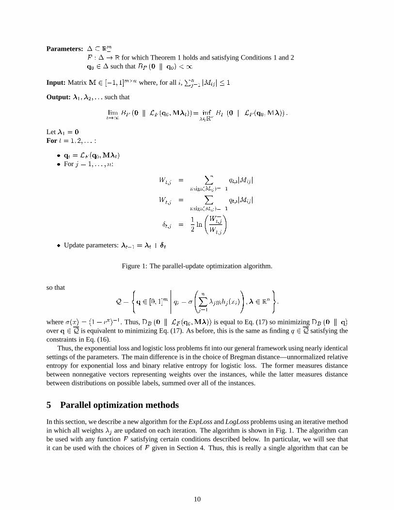
5 Parallel optimization methods
In this section, we describe a new algorithm for theExpLossandLogLossproblems using an iterative methodin which all weights�
j
are updated on each iteration. The algorithm is shown in Fig.1. The algorithm canbe used with any functionF satisfying certain conditions described below. In particular, we will see thatit can be used with the choices ofF given in Section 4. Thus, this is really a single algorithm that can be
10
used for both loss-minimization problems by setting the parameters appropriately. Note that, without lossof generality, we assume in this section that for all instancesi,
P
n
j=1
jM
ij
j � 1.The algorithm is very simple. On each iteration, the vector�
t
is computed as shown and added to theparameter vector�
t
. We assume for all our algorithms that the inputs are such that infinite-valued updatesnever occur.
This algorithm is new for both minimization problems. Optimization methods forExpLoss, notablyAdaBoost, have generally involved updates of one feature ata time. Parallel-update methods forLogLossare well known (see, for example, (Darroch & Ratcliff, 1972;Della Pietra et al., 1997)). However, ourupdates take a different form from the usual updates derivedfor logistic models. We discuss the differencesin Section 9.
A useful point is that the distributionqt+1
is a simple function of the previous distributionqt
. By Eq. (8),
q
t+1
= L
F
(q
0
;M(�
t
+ �
t
)) = L
F
(L
F
(q
0
;M�
t
);M�
t
)
= L
F
(q
t
;M�
t
): (20)
This gives
q
t+1;i
=
8
<
:
q
t;i
exp
�
�
P
n
j=1
�
t;j
M
ij
�
forExpLoss
q
t;i
h
(1� q
t;i
) exp
�
P
n
j=1
�
t;j
M
ij
�
+ q
t;i
i
�1
forLogLoss:(21)
We will prove next that the algorithm given in Fig. 1 converges to optimality for either loss. We prove thisabstractly for any matrixM and vectorq
0
, and for any functionF satisfying Theorem 1 and the followingconditions:
Condition 1 For anyv 2 R
m, q 2 �,
B
F
(0 k L
F
(q;v))�B
F
(0 k q) �
m
X
i=1
q
i
(e
�v
i
� 1):
Condition 2 For anyc <1, the set
fq 2 � j B
F
(0 k q) � cg
is bounded.
We will show later that the choices ofF given in Section 4 satisfy these conditions which will allowusto prove convergence forExpLossandLogLoss.
To prove convergence, we use the auxiliary-function technique of Della Pietra, Della Pietra and Laf-ferty (1997). Very roughly, the idea of the proof is to derivea nonnegative lower bound called an auxiliaryfunction on how much the loss decreases on each iteration. Since the loss never increases and is lowerbounded by zero, the auxiliary function must converge to zero. The final step is to show that when theauxiliary function is zero, the constraints defining the setP must be satisfied, and therefore, by Theorem 1,we must have converged to optimality.
More formally, we define anauxiliary functionfor a sequenceq1
;q
2
; : : : and matrixM to be a contin-uous functionA : �! R satisfying the two conditions:
B
F
(0 k q
t+1
)�B
F
(0 k q
t
) � A(q
t
) � 0 (22)
andA(q) = 0) q
T
M = 0
T
: (23)
Before proving convergence of specific algorithms, we provethe following lemma which shows, roughly,that if a sequence has an auxiliary function, then the sequence converges to the optimum pointq
?
. Thus,proving convergence of a specific algorithm reduces to simply finding an auxiliary function.
11
Lemma 2 LetA be an auxiliary function forq1
;q
2
; : : : and matrixM. Assume theqt
’s lie in a compactsubspace ofQ whereQ is as in Eq. (10). AssumF satisfies Theorem 1. Then
lim
t!1
q
t
= q
?
:
= argmin
q2Q
B
F
(0 k q) :
Note that theqt
’s will lie in a compact subspace ofQ if Condition 2 holds andBF
(0 k q
1
) < 1. Inthe algorithm in Figure 1, and in general in the algorithms inthis paper,�
1
= 0, so thatq1
= q
0
and theconditionB
F
(0 k q
0
) <1 impliesBF
(0 k q
1
) <1. BF
(0 k q
0
) <1 is an input condition for allof the algorithms in this paper.Proof: By condition (22),B
F
(0 k q
t
) is a nonincreasing sequence. As is the case for all Bregman dis-tances,B
F
(0 k q
t
) is also bounded below by zero. Therefore, the sequence of differences
B
F
(0 k q
t+1
)�B
F
(0 k q
t
)
must converge to zero. Using the condition of Eq. (22), this means thatA(qt
) must also converge to zero.Because we assume that theq
t
’s lie in a compact space, the sequence ofq
t
’s must have a subsequenceconverging to some point^q 2 �. By continuity ofA, we haveA(^q) = 0. Therefore,^q 2 P from thecondition given by Eq. (23), whereP is as in Eq. (7). On the other hand,^q is the limit of a sequence ofpoints inQ so^
q 2 Q. Thus,^q 2 P \Q so^q = q
?
by Theorem 1.This argument and the uniqueness ofq
?
show that theqt
’s have only a single limit pointq?
. Supposethat the entire sequence did not converge toq
?
. Then we could find an open setB containingq?
such thatfq
1
;q
2
; : : :g�B contains infinitely many points and therefore has a limit point which must be in the closedset� � B and so must be different fromq
?
. This, we have already argued, is impossible. Therefore, theentire sequence converges toq
?
.We can now apply this lemma to prove the convergence of the algorithm of Fig. 1.
Theorem 3 LetF satisfy Theorem 1 and Conditions 1 and 2, and assume thatB
F
(0 k q
0
) <1. Let thesequences�
1
;�
2
; : : : andq1
;q
2
; : : : be generated by the algorithm of Fig. 1. Then
lim
t!1
q
t
= argmin
q2Q
B
F
(0 k q)
whereQ is as in Eq. (10). That is,
lim
t!1
B
F
(0 k L
F
(q
0
;M�
t
))= inf
�2R
n
B
F
(0 k L
F
(q
0
;M�)) :
Proof: Let
W
+
j
(q) =
X
i:sign(M
ij
)=+1
q
i
jM
ij
j
W
�
j
(q) =
X
i:sign(M
ij
)=�1
q
i
jM
ij
j
so thatW+
t;j
= W
+
j
(q
t
) andW�
t;j
= W
�
j
(q
t
). We claim that the function
A(q) = �
n
X
j=1
�
q
W
+
j
(q)�
q
W
�
j
(q)
�
2
is an auxiliary function forq1
;q
2
; : : :. Clearly,A is continuous and nonpositive.
12
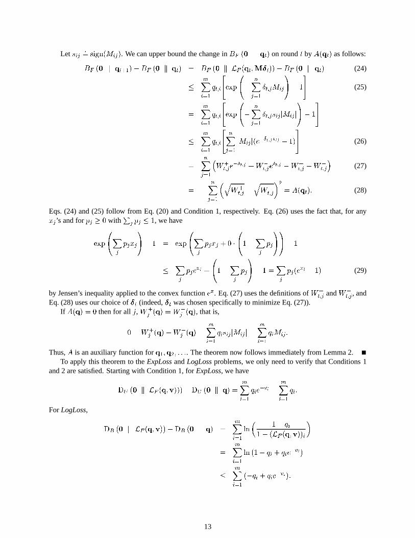
Let sij
:
= sign(M
ij
). We can upper bound the change inBF
(0 k q
t
) on roundt byA(qt
) as follows:
B
F
(0 k q
t+1
)�B
F
(0 k q
t
) = B
F
(0 k L
F
(q
t
;M�
t
))�B
F
(0 k q
t
) (24)
�
m
X
i=1
q
t;i
2
4
exp
0
@
�
n
X
j=1
�
t;j
M
ij
1
A
� 1
3
5 (25)
=
m
X
i=1
q
t;i
2
4
exp
0
@
�
n
X
j=1
�
t;j
s
ij
jM
ij
j
1
A
� 1
3
5
�
m
X
i=1
q
t;i
2
4
n
X
j=1
jM
ij
j(e
��
t;j
s
ij
� 1)
3
5 (26)
=
n
X
j=1
�
W
+
t;j
e
��
t;j
+W
�
t;j
e
�
t;j
�W
+
t;j
�W
�
t;j
�
(27)
= �
n
X
j=1
�
q
W
+
t;j
�
q
W
�
t;j
�
2
= A(q
t
): (28)
Eqs. (24) and (25) follow from Eq. (20) and Condition 1, respectively. Eq. (26) uses the fact that, for anyx
j
’s and forpj
� 0 withP
j
p
j
� 1, we have
exp
0
@
X
j
p
j
x
j
1
A
� 1 = exp
0
@
X
j
p
j
x
j
+ 0 �
0
@
1�
X
j
p
j
1
A
1
A
� 1
�
X
j
p
j
e
x
i
+
0
@
1�
X
j
p
j
1
A
� 1 =
X
j
p
j
(e
x
i
� 1) (29)
by Jensen’s inequality applied to the convex functione
x. Eq. (27) uses the definitions ofW+
t;j
andW�
t;j
, andEq. (28) uses our choice of�
t
(indeed,�t
was chosen specifically to minimize Eq. (27)).If A(q) = 0 then for allj, W+
j
(q) = W
�
j
(q), that is,
0 = W
+
j
(q)�W
�
j
(q) =
m
X
i=1
q
i
s
ij
jM
ij
j =
m
X
i=1
q
i
M
ij
:
Thus,A is an auxiliary function forq1
;q
2
; : : :. The theorem now follows immediately from Lemma 2.To apply this theorem to theExpLossandLogLossproblems, we only need to verify that Conditions 1
and 2 are satisfied. Starting with Condition 1, forExpLoss, we have
D
U
(0 k L
F
(q;v)))�D
U
(0 k q) =
m
X
i=1
q
i
e
�v
i
�
m
X
i=1
q
i
:
For LogLoss,
D
B
(0 k L
F
(q;v))�D
B
(0 k q) =
m
X
i=1
ln
�
1� q
i
1� (L
F
(q;v))
i
�
=
m
X
i=1
ln
�
1� q
i
+ q
i
e
�v
i
�
�
m
X
i=1
�
�q
i
+ q
i
e
�v
i
�
:
13
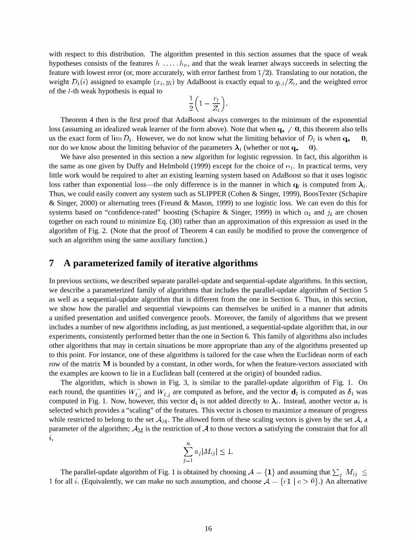
The first and second equalities use Eqs. (18) and (19), respectively. The final inequality uses1 + x � e
x forall x.
Condition 2 holds trivially forLogLosssince� = [0; 1]
m is bounded. ForExpLoss, if BF
(0 k q) =
D
U
(0 k q) � c thenm
X
i=1
q
i
� c
which clearly defines a bounded subset ofR
m
+
.Note that while Condition 1 holds for the loss functions we are considering, it may not hold for all
Bregman distances. Lafferty, Della Pietra and Della Pietra(1997) describe parallel update algorithms forBregman distances, using the auxiliary function technique. Their method does not require Condition 1, andtherefore applies to arbitrary Bregman distances; however, each iteration of the algorithm requires solutionof a system of equations that requires a numerical search technique such as Newton’s method.
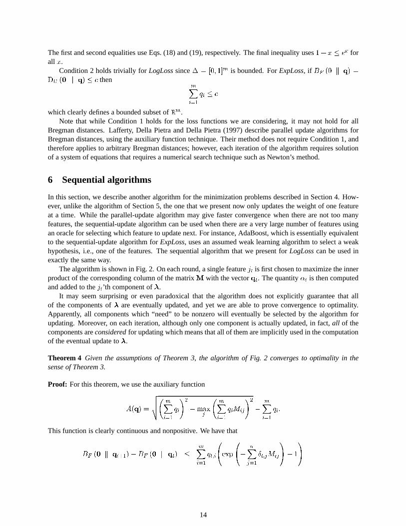
6 Sequential algorithms
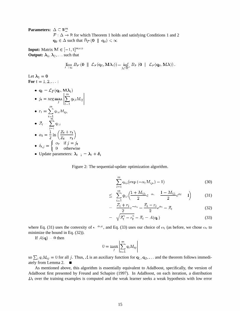
In this section, we describe another algorithm for the minimization problems described in Section 4. How-ever, unlike the algorithm of Section 5, the one that we present now only updates the weight of one featureat a time. While the parallel-update algorithm may give faster convergence when there are not too manyfeatures, the sequential-update algorithm can be used whenthere are a very large number of features usingan oracle for selecting which feature to update next. For instance, AdaBoost, which is essentially equivalentto the sequential-update algorithm forExpLoss, uses an assumed weak learning algorithm to select a weakhypothesis, i.e., one of the features. The sequential algorithm that we present forLogLosscan be used inexactly the same way.
The algorithm is shown in Fig. 2. On each round, a single feature jt
is first chosen to maximize the innerproduct of the corresponding column of the matrixM with the vectorq
t
. The quantity�t
is then computedand added to thej
t
’th component of�.It may seem surprising or even paradoxical that the algorithm does not explicitly guarantee that all
of the components of� are eventually updated, and yet we are able to prove convergence to optimality.Apparently, all components which “need” to be nonzero will eventually be selected by the algorithm forupdating. Moreover, on each iteration, although only one component is actually updated, in fact,all of thecomponents areconsideredfor updating which means that all of them are implicitly usedin the computationof the eventual update to�.
Theorem 4 Given the assumptions of Theorem 3, the algorithm of Fig. 2 converges to optimality in thesense of Theorem 3.
Proof: For this theorem, we use the auxiliary function
A(q) =
v
u
u
t
m
X
i=1
q
i
!
2
�max
j
m
X
i=1
q
i
M
ij
!
2
�
m
X
i=1
q
i
:
This function is clearly continuous and nonpositive. We have that
B
F
(0 k q
t+1
)�B
F
(0 k q
t
) �
m
X
i=1
q
t;i
0
@
exp
0
@
�
n
X
j=1
�
t;j
M
ij
1
A
� 1
1
A
14
Parameters: � � R
m
+
F : �! R for which Theorem 1 holds and satisfying Conditions 1 and 2q
0
2 � such thatBF
(0 k q
0
) <1
Input: Matrix M 2 [�1; 1]
m�n
Output: �1
;�
2
; : : : such that
lim
t!1
B
F
(0 k L
F
(q
0
;M�
t
))= inf
�2R
n
B
F
(0 k L
F
(q
0
;M�)) :
Let�1
= 0
For t = 1; 2; : : : :
� q
t
= L
F
(q
0
;M�
t
)
� j
t
= argmax
j
�
�
�
�
�
m
X
i=1
q
t;i
M
ij
�
�
�
�
�
� r
t
=
m
X
i=1
q
t;i
M
ij
t
� Z
t
=
m
X
i=1
q
t;i
� �
t
=
1
2
ln
�
Z
t
+ r
t
Z
t
� r
t
�
� �
t;j
=
(
�
t
if j = j
t
0 otherwise� Update parameters:�
t+1
= �
t
+ �
t
Figure 2: The sequential-update optimization algorithm.
=
m
X
i=1
q
t;i
(exp (��
t
M
ij
t
)� 1) (30)
�
m
X
i=1
q
t;i
�
1 +M
ij
t
2
e
��
t
+
1�M
ij
t
2
e
�
t
� 1
�
(31)
=
Z
t
+ r
t
2
e
��
t
+
Z
t
� r
t
2
e
�
t
� Z
t
(32)
=
q
Z
2
t
� r
2
t
� Z
t
= A(q
t
) (33)
where Eq. (31) uses the convexity ofe��tx, and Eq. (33) uses our choice of�t
(as before, we chose�t
tominimize the bound in Eq. (32)).
If A(q) = 0 then
0 = max
j
�
�
�
�
�
m
X
i=1
q
i
M
ij
�
�
�
�
�
soP
i
q
i
M
ij
= 0 for all j. Thus,A is an auxiliary function forq1
;q
2
; : : : and the theorem follows immedi-ately from Lemma 2.
As mentioned above, this algorithm is essentially equivalent to AdaBoost, specifically, the version ofAdaBoost first presented by Freund and Schapire (1997). In AdaBoost, on each iteration, a distributionD
t
over the training examples is computed and the weak learner seeks a weak hypothesis with low error
15
with respect to this distribution. The algorithm presentedin this section assumes that the space of weakhypotheses consists of the featuresh
1
; : : : ; h
n
, and that the weak learner always succeeds in selecting thefeature with lowest error (or, more accurately, with error farthest from1=2). Translating to our notation, theweightD
t
(i) assigned to example(xi
; y
i
) by AdaBoost is exactly equal toqt;i
=Z
t
, and the weighted errorof thet-th weak hypothesis is equal to
1
2
�
1�
r
t
Z
t
�
:
Theorem 4 then is the first proof that AdaBoost always converges to the minimum of the exponentialloss (assuming an idealized weak learner of the form above).Note that whenq
?
6= 0, this theorem also tellsus the exact form oflimD
t
. However, we do not know what the limiting behavior ofD
t
is whenq?
= 0,nor do we know about the limiting behavior of the parameters�
t
(whether or notq?
= 0).We have also presented in this section a new algorithm for logistic regression. In fact, this algorithm is
the same as one given by Duffy and Helmbold (1999) except for the choice of�t
. In practical terms, verylittle work would be required to alter an existing learning system based on AdaBoost so that it uses logisticloss rather than exponential loss—the only difference is inthe manner in whichq
t
is computed from�t
.Thus, we could easily convert any system such as SLIPPER (Cohen & Singer, 1999), BoosTexter (Schapire& Singer, 2000) or alternating trees (Freund & Mason, 1999) to use logistic loss. We can even do this forsystems based on “confidence-rated” boosting (Schapire & Singer, 1999) in which�
t
and jt
are chosentogether on each round to minimize Eq. (30) rather than an approximation of this expression as used in thealgorithm of Fig. 2. (Note that the proof of Theorem 4 can easily be modified to prove the convergence ofsuch an algorithm using the same auxiliary function.)
7 A parameterized family of iterative algorithms
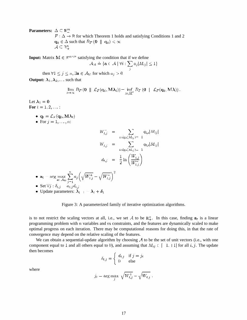
In previous sections, we described separate parallel-update and sequential-update algorithms. In this section,we describe a parameterized family of algorithms that includes the parallel-update algorithm of Section 5as well as a sequential-update algorithm that is different from the one in Section 6. Thus, in this section,we show how the parallel and sequential viewpoints can themselves be unified in a manner that admitsa unified presentation and unified convergence proofs. Moreover, the family of algorithms that we presentincludes a number of new algorithms including, as just mentioned, a sequential-update algorithm that, in ourexperiments, consistently performed better than the one inSection 6. This family of algorithms also includesother algorithms that may in certain situations be more appropriate than any of the algorithms presented upto this point. For instance, one of these algorithms is tailored for the case when the Euclidean norm of eachrow of the matrixM is bounded by a constant, in other words, for when the feature-vectors associated withthe examples are known to lie in a Euclidean ball (centered atthe origin) of bounded radius.
The algorithm, which is shown in Fig. 3, is similar to the parallel-update algorithm of Fig. 1. Oneach round, the quantitiesW+
t;j
andW�
t;j
are computed as before, and the vectord
t
is computed as�t
wascomputed in Fig. 1. Now, however, this vectord
t
is not added directly to�t
. Instead, another vectorat
isselected which provides a “scaling” of the features. This vector is chosen to maximize a measure of progresswhile restricted to belong to the setA
M
. The allowed form of these scaling vectors is given by the setA, aparameter of the algorithm;A
M
is the restriction ofA to those vectorsa satisfying the constraint that for alli,
n
X
j=1
a
j
jM
ij
j � 1:
The parallel-update algorithm of Fig. 1 is obtained by choosingA = f1g and assuming thatP
j
jM
ij
j �
1 for all i. (Equivalently, we can make no such assumption, and chooseA = fc1 j c > 0g.) An alternative
16
Parameters: � � R
m
+
F : �! R for which Theorem 1 holds and satisfying Conditions 1 and 2q
0
2 � such thatBF
(0 k q
0
) <1
A � R
n
+
Input: Matrix M 2 R
m�n satisfying the condition that if we defineA
M
:
= fa 2 A j 8i :
X
j
a
j
jM
ij
j � 1g
then81 � j � n;9a 2 A
M
for whichaj
> 0
Output: �1
;�
2
; : : : such that
lim
t!1
B
F
(0 k L
F
(q
0
;M�
t
))= inf
�2R
n
B
F
(0 k L
F
(q
0
;M�)) :
Let�1
= 0
For t = 1; 2; : : : :
� q
t
= L
F
(q
0
;M�
t
)
� For j = 1; : : : ; n:
W
+
t;j
=
X
i:sign(M
ij
)=+1
q
t;i
jM
ij
j
W
�
t;j
=
X
i:sign(M
ij
)=�1
q
t;i
jM
ij
j
d
t;j
=
1
2
ln
W
+
t;j
W
�
t;j
!
� a
t
= arg max
a2A
M
n
X
j=1
a
j
�
q
W
+
t;j
�
q
W
�
t;j
�
2
� Set8j : �t;j
= a
t;j
d
t;j
� Update parameters:�t+1
= �
t
+ �
t
Figure 3: A parameterized family of iterative optimizationalgorithms.
is to not restrict the scaling vectors at all, i.e., we setA to beRn+
. In this case, findingat
is a linearprogramming problem withn variables andm constraints, and the features are dynamically scaled to makeoptimal progress on each iteration. There may be computational reasons for doing this, in that the rate ofconvergence may depend on the relative scaling of the features.
We can obtain a sequential-update algorithm by choosingA to be the set of unit vectors (i.e., with onecomponent equal to1 and all others equal to0), and assuming thatM
ij
2 [�1;+1] for all i; j. The updatethen becomes
�
t;j
=
(
d
t;j
if j = j
t
0 else
where
j
t
= argmax
j
�
�
�
�
q
W
+
t;j
�
q
W
�
t;j
�
�
�
�
:
17
Another interesting case is when we assume thatP
j
M
2
ij
� 1 for all i. It is then natural to choose
A = fa 2 R
n
+
j jjajj
2
= 1g
which ensures thatAM
= A. Then the maximization overAM
can be solved analytically giving the update
�
t;j
=
b
j
d
t;j
jjbjj
2
wherebj
=
�q
W
+
t;j
�
q
W
�
t;j
�
2
. This idea generalizes easily to the case in whichP
j
jM
ij
j
p
� 1 and
jjajj
q
= 1 for any dual normsp andq (1p
+
1
q
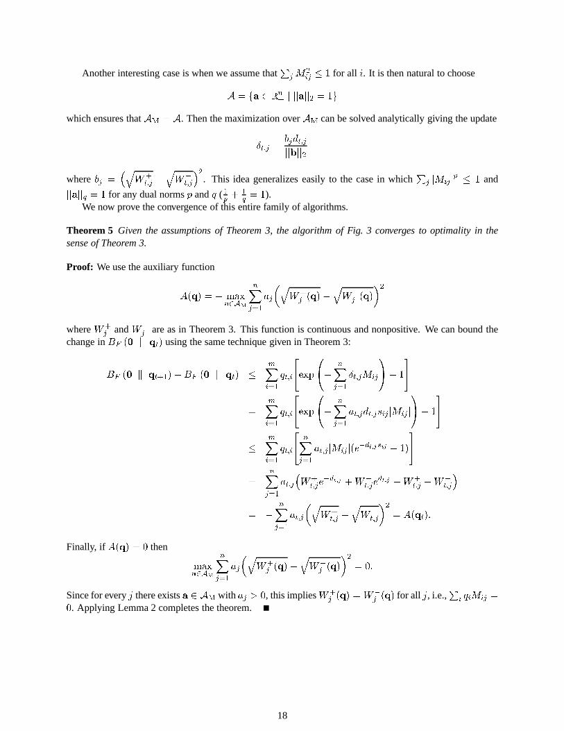
= 1).We now prove the convergence of this entire family of algorithms.
Theorem 5 Given the assumptions of Theorem 3, the algorithm of Fig. 3 converges to optimality in thesense of Theorem 3.
Proof: We use the auxiliary function
A(q) = � max
a2A
M
n
X
j=1
a
j
�
q
W
+
j
(q)�
q
W
�
j
(q)
�
2
whereW+
j
andW�
j
are as in Theorem 3. This function is continuous and nonpositive. We can bound thechange inB
F
(0 k q
t
) using the same technique given in Theorem 3:
B
F
(0 k q
t+1
)�B
F
(0 k q
t
) �
m
X
i=1
q
t;i
2
4
exp
0
@
�
n
X
j=1
�
t;j
M
ij
1
A
� 1
3
5
=
m
X
i=1
q
t;i
2
4
exp
0
@
�
n
X
j=1
a
t;j
d
t;j
s
ij
jM
ij
j
1
A
� 1
3
5
�
m
X
i=1
q
t;i
2
4
n
X
j=1
a
t;j
jM
ij
j(e
�d
t;j
s
ij
� 1)
3
5
=
n
X
j=1
a
t;j
�
W
+
t;j
e
�d
t;j
+W
�
t;j
e
d
t;j
�W
+
t;j
�W
�
t;j
�
= �
n
X
j=1
a
t;j
�
q
W
+
t;j
�
q
W
�
t;j
�
2
= A(q
t
):
Finally, if A(q) = 0 then
max
a2A
M
n
X
j=1
a
j
�
q
W
+
j
(q)�
q
W
�
j
(q)
�
2
= 0:
Since for everyj there existsa 2 AM
with aj
> 0, this impliesW+
j
(q) = W
�
j
(q) for all j, i.e.,P
i
q
i
M
ij
=
0. Applying Lemma 2 completes the theorem.
18
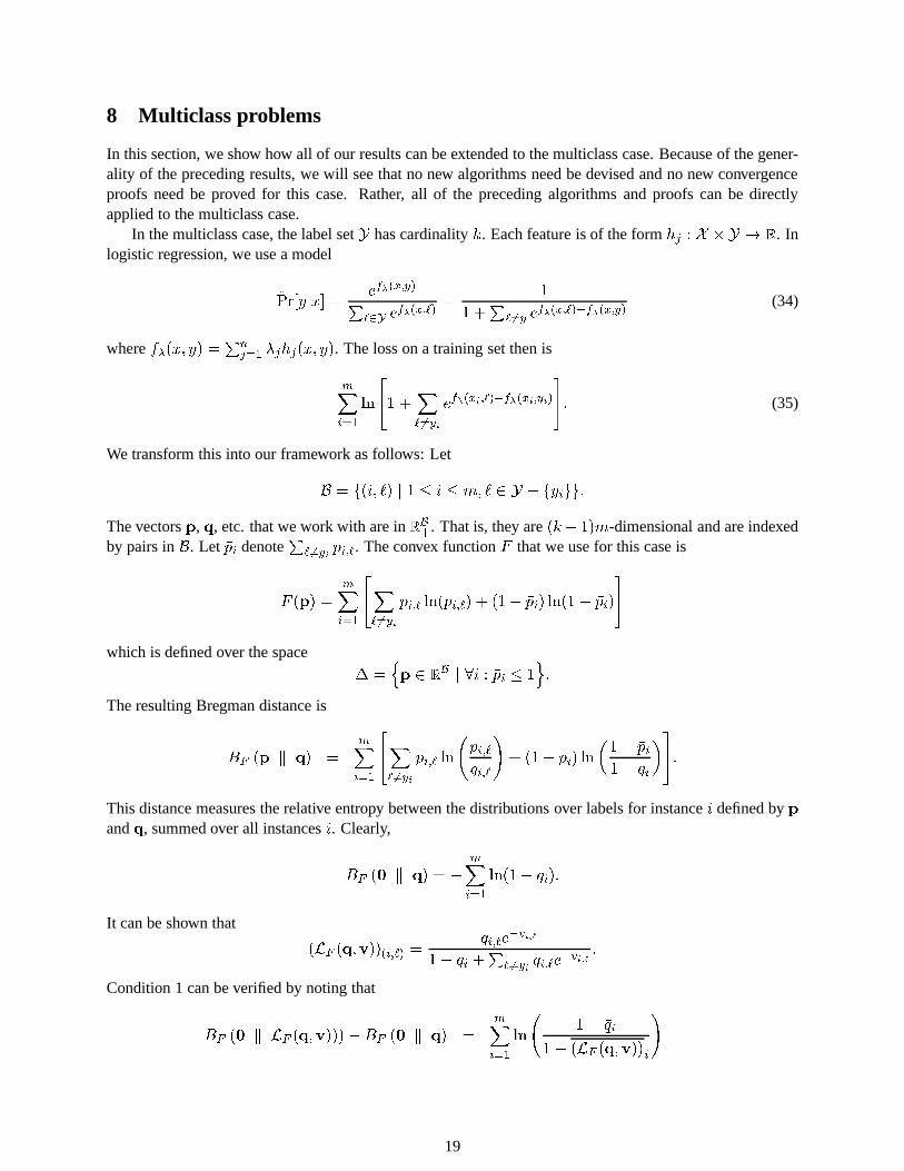
8 Multiclass problems
In this section, we show how all of our results can be extendedto the multiclass case. Because of the gener-ality of the preceding results, we will see that no new algorithms need be devised and no new convergenceproofs need be proved for this case. Rather, all of the preceding algorithms and proofs can be directlyapplied to the multiclass case.
In the multiclass case, the label setY has cardinalityk. Each feature is of the formhj
: X �Y ! R. Inlogistic regression, we use a model
^
Pr[yjx] =
e
f
�
(x;y)
P
`2Y
e
f
�
(x;`)
=
1
1 +
P
`6=y
e
f
�
(x;`)�f
�
(x;y)
(34)
wheref�
(x; y) =
P
n
j=1
�
j
h
j
(x; y). The loss on a training set then is
m
X
i=1
ln
2
4
1 +
X
`6=y
i
e
f
�
(x
i
;`)�f
�
(x
i
;y
i
)
3
5
: (35)
We transform this into our framework as follows: Let
B = f(i; `) j 1 � i � m; ` 2 Y � fy
i
gg:
The vectorsp, q, etc. that we work with are inRB+
. That is, they are(k� 1)m-dimensional and are indexedby pairs inB. Let �p
i
denoteP
`6=y
i
p
i;`
. The convex functionF that we use for this case is
F (p) =
m
X
i=1
2
4
X
`6=y
i
p
i;`
ln(p
i;`
) + (1� �p
i
) ln(1� �p
i
)
3
5
which is defined over the space� =
n
p 2 R
B
+
j 8i : �p
i
� 1
o
:
The resulting Bregman distance is
B
F
(p k q) =
m
X
i=1
2
4
X
`6=y
i
p
i;`
ln
p
i;`
q
i;`
!
+ (1� �p
i
) ln
�
1� �p
i
1� �q
i
�
3
5
:
This distance measures the relative entropy between the distributions over labels for instancei defined bypandq, summed over all instancesi. Clearly,
B
F
(0 k q) = �
m
X
i=1
ln(1� �q
i
):
It can be shown that
(L
F
(q;v))
(i;`)
=
q
i;`
e
�v
i;`
1� �q
i
+
P
`6=y
i
q
i;`
e
�v
i;`
:
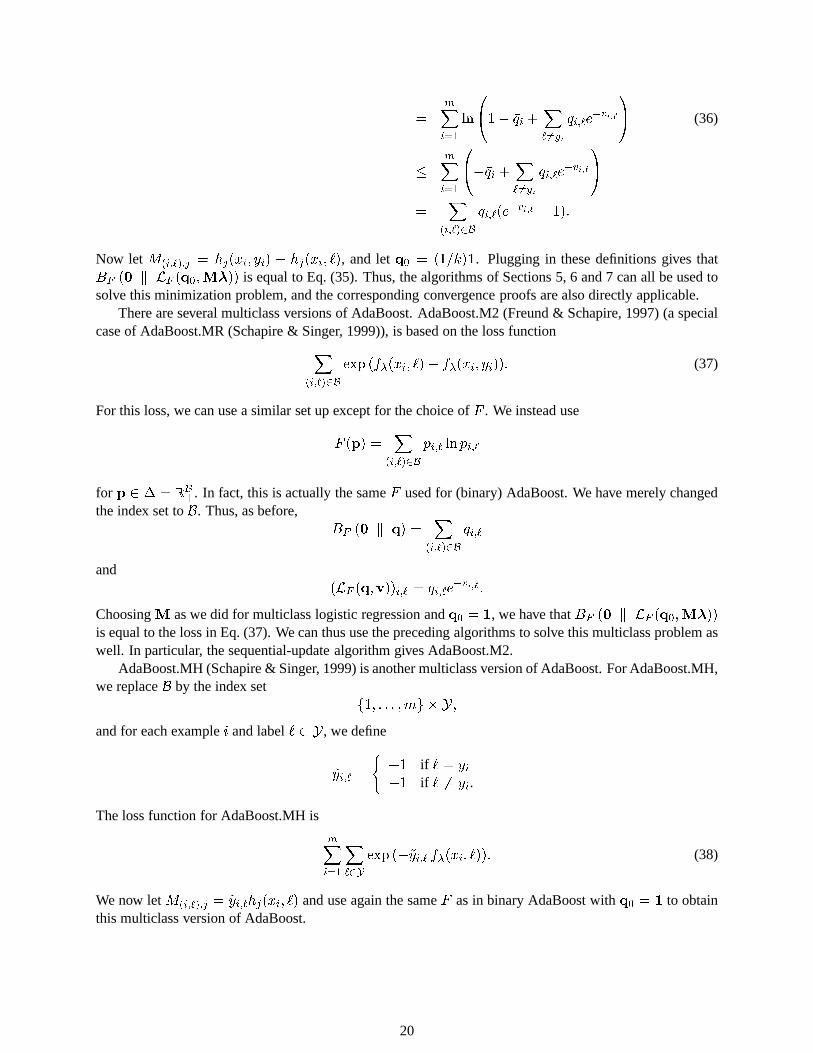
Condition 1 can be verified by noting that
B
F
(0 k L
F
(q;v)))�B
F
(0 k q) =
m
X
i=1
ln
1� �q
i
1� (L
F
(q;v))
i
!
19
=
m
X
i=1
ln
0
@
1� �q
i
+
X
`6=y
i
q
i;`
e
�v
i;`
1
A (36)
�
m
X
i=1
0
@
��q
i
+
X
`6=y
i
q
i;`
e
�v
i;`
1
A
=
X
(i;`)2B
q
i;`
(e
�v
i;`
� 1):
Now letM(i;`);j
= h
j
(x
i
; y
i
) � h
j
(x
i
; `), and letq0
= (1=k)1. Plugging in these definitions gives thatB
F
(0 k L
F
(q
0
;M�)) is equal to Eq. (35). Thus, the algorithms of Sections 5, 6 and7 can all be used tosolve this minimization problem, and the corresponding convergence proofs are also directly applicable.
There are several multiclass versions of AdaBoost. AdaBoost.M2 (Freund & Schapire, 1997) (a specialcase of AdaBoost.MR (Schapire & Singer, 1999)), is based on the loss function
X
(i;`)2B
exp (f
�
(x
i
; `)� f
�
(x
i
; y
i
)): (37)
For this loss, we can use a similar set up except for the choiceof F . We instead use
F (p) =
X
(i;`)2B
p
i;`
ln p
i;`
for p 2 � = R
B
+
. In fact, this is actually the sameF used for (binary) AdaBoost. We have merely changedthe index set toB. Thus, as before,
B
F
(0 k q) =
X
(i;`)2B
q
i;`
and(L
F
(q;v))
i;`
= q
i;`
e
�v
i;`
:
ChoosingM as we did for multiclass logistic regression andq0
= 1, we have thatBF
(0 k L
F
(q
0
;M�))
is equal to the loss in Eq. (37). We can thus use the preceding algorithms to solve this multiclass problem aswell. In particular, the sequential-update algorithm gives AdaBoost.M2.
AdaBoost.MH (Schapire & Singer, 1999) is another multiclass version of AdaBoost. For AdaBoost.MH,we replaceB by the index set
f1; : : : ;mg � Y;
and for each examplei and label 2 Y, we define
~y
i;`
=
(
+1 if ` = y
i
�1 if ` 6= y
i
.
The loss function for AdaBoost.MH is
m
X
i=1
X
`2Y
exp (�~y
i;`
f
�
(x
i
; `)): (38)
We now letM(i;`);j
= ~y
i;`
h
j
(x
i
; `) and use again the sameF as in binary AdaBoost withq0
= 1 to obtainthis multiclass version of AdaBoost.
20
9 A comparison to iterative scaling
In this section, we describe the generalized iterative scaling (GIS) procedure of Darroch and Ratcliff (1972)for comparison to our algorithms. We largely follow the description of GIS given by Berger, Della Pietraand Della Pietra (1996) for the multiclass case. To make the comparison as stark as possible, we presentGIS in our notation and prove its convergence using the methods developed in previous sections. In doingso, we are also able to relax one of the key assumptions traditionally used in studying GIS.
We adopt the notation and set-up used for multiclass logistic regression in Section 8. (To our knowledge,there is no analog of GIS for the exponential loss so we only consider the case of logistic loss.) We alsoextend this notation by definingq
i;y
i
= 1 � �q
i
so thatqi;`
is now defined for all 2 Y. Moreover, it can beverified thatq
i;`
=
^
Pr[`jx
i
] as defined in Eq. (34) ifq = L
F
(q
0
;M�).In GIS, the following assumptions regarding the features are usually made:
8i; j; ` : h
j
(x
i
; `) � 0 and 8i; ` :
n
X
j=1
h
j
(x
i
; `) = 1 :
In this section, we prove that GIS converges with the second condition replaced by a milder one, namely,that
8i; ` :
n
X
j=1
h
j
(x
i
; `) � 1 :
Since, in the multiclass case, a constant can be added to all featureshj
without changing the model or lossfunction, and since the features can be scaled by any constant, the two assumptions we consider clearlycan be made to hold without loss of generality. The improved iterative scaling algorithm of Della Pietra,Della Pietra and Lafferty (1997) also requires only these milder assumptions but is more complicated toimplement, requiring a numerical search (such as Newton-Raphson) for each feature on each iteration.
GIS works much like the parallel-update algorithm of Section 5 with F , M andq0
as defined formulticlass logistic regression in Section 8. The only difference is in the computation of the vector of updates�
t
, for which GIS requires direct access to the featuresh
j
. Specifically, in GIS,�t
is defined to be
�
t;j
= ln
H
j
I
j
(q
t
)
!
where
H
j
=
m
X
i=1
h
j
(x
i
; y
i
)
I
j
(q) =
m
X
i=1
X
`2Y
q
i;`
h
j
(x
i
; `):
Clearly, these updates are quite different from the updatesdescribed in this paper.Using notation from Sections 5 and 8, we can reformulateI
j
(q) within our framework as follows:
I
j
(q) =
m
X
i=1
X
`2Y
q
i;`
h
j
(x
i
; `)
=
m
X
i=1
h
j
(x
i
; y
i
)
21
+
m
X
i=1
X
`2Y
q
i;`
[h
j
(x
i
; `)� h
j
(x
i
; y
i
)]
= H
j
�
X
(i;`)2B
q
i;`
M
(i;`);j
= H
j
� (W
+
j
(q)�W
�
j
(q)) ; (39)
where we defineB = f(i; `) j 1 � i � m; ` 2 Y � fy
i
gg, as in the case of logistic regression.We can now prove the convergence of these updates using the usual auxiliary function method.
Theorem 6 LetF , M andq0
be as above. Then the modified GIS algorithm described above converges tooptimality in the sense of Theorem 3.
Proof: We will show that
A(q)
:
= �D
U
(hH
1
; : : : ;H
n
i k hI
1
(q); : : : ; I
n
(q)i)
= �
n
X
j=1
H
j
ln
H
j
I
j
(q)
+ I
j
(q)�H
j
!
(40)
is an auxiliary function for the vectorsq1
;q
2
; : : : computed by GIS. Clearly,A is continuous, and the usualnonnegativity properties of unnormalized relative entropy imply thatA(q) � 0 with equality if and only ifH
j
= I
j
(q) for all j. From Eq. (39),Hj
= I
j
(q) if and only ifW+
j
(q) = W
�
j
(q). Thus,A(q) = 0 impliesthat the constraintsqTM = 0
T as in the proof of Theorem 3. All that remains to be shown is that
B
F
(0 k L
F
(q;M�))�B
F
(0 k q) � A(q) (41)
where
�
j
= ln
H
j
I
j
(q)
!
:
We introduce the notation
�
i
(`) =
n
X
j=1
�
j
h
j
(x
i
; `);
and then rewrite the left hand side of Eq. (41) as follows using Eq. (36):
B
F
(0 k L
F
(q;M�))�B
F
(0 k q) =
m
X
i=1
ln
0
@
q
i;y
i
+
X
`6=y
i
q
i;`
exp
0
@
�
n
X
j=1
�
j
M
(i;`);j
1
A
1
A
= �
m
X
i=1
�
i
(y
i
)
+
m
X
i=1
ln
2
4
e
�
i
(y
i
)
0
@
q
i;y
i
+
X
`6=y
i
q
i;`
e
�
P
n
j=1
�
j
M
(i;`);j
1
A
3
5
:
(42)
Plugging in definitions, the first term of Eq. (42) can be written as
m
X
i=1
�
i
(y
i
) =
n
X
j=1
"
ln
H
j
I
j
(q)
!
m
X
i=1
h
j
(x
i
; y
i
)
#
=
n
X
j=1
H
j
ln
H
j
I
j
(q)
!
: (43)
22
Next we derive an upper bound on the second term of Eq. (42):
m
X
i=1
ln
2
4
e
�
i
(y
i
)
0
@
q
i;y
i
+
X
`6=y
i
q
i;`
e
�
P
n
j=1
�
j
M
(i;`);j
1
A
3
5
=
m
X
i=1
ln
0
@
q
i;y
i
e
�
i
(y
i
)
+
X
`6=y
i
q
i;`
e
�
i
(`)
1
A
=
m
X
i=1
ln
0
@
X
`2Y
q
i;`
e
�
i
(`)
1
A
�
m
X
i=1
0
@
X
`2Y
q
i;`
e
�
i
(`)
� 1
1
A (44)
=
m
X
i=1
X
`2Y
q
i;`
2
4
exp
0
@
n
X
j=1
h
j
(x
i
; `)�
j
1
A
� 1
3
5 (45)
�
m
X
i=1
X
`2Y
q
i;`
n
X
j=1
h
j
(x
i
; `)(e
�
j
� 1) (46)
=
m
X
i=1
X
`2Y
q
i;`
n
X
j=1
h
j
(x
i
; `)
H
j
I
j
(q)
� 1
!
(47)
=
n
X
j=1
H
j
I
j
(q)
� 1
!
m
X
i=1
X
`2Y
q
i;`
h
j
(x
i
; `)
=
n
X
j=1
(H
j
� I
j
(q)) : (48)
Eq. (44) follows from the log boundlnx � x � 1. Eq. (46) uses Eq. (29) and our assumption on the formof theh
j
’s. Eq. (47) follows from our definition of the update�.Finally, combining Eqs. (40), (42), (43) and (48) gives Eq. (41) completing the proof.It is clear that the differences between GIS and the updates given in this paper stem from Eq. (42), which
is derived fromlnx = �C + ln
�
e
C
x
�
, with C = �
i
(y
i
) on thei’th term in the sum. This choice ofC
effectively means that the log bound is taken at a different point (lnx = �C+ln
�
e
C
x
�
� �C+ e
C
x�1).
In this more general case, the bound is exact atx = e
�C ; hence, varyingC varies where the bound is taken,and thereby varies the updates.
10 Discussion
In this section we discuss various notions of convergence ofAdaBoost, relating the work in this paper toprevious work on boosting, and in particular to previous work on the convergence properties of AdaBoost.
The algorithms in this paper define a sequence of parameter settings�1
;�
2
; : : :. There are various func-tions of the parameter settings, for which sequences are therefore also defined and for which convergenceproperties may be of interest. For instance, one can investigate convergence in value, i.e., convergence ofthe exponential loss function, as defined in Eq. (14); convergence of either the unnormalized distributionsq
t
or the normalized distributionsqt
=(
P
i
q
t
i
), over the training examples; and convergence in parameters,that is, convergence of�
t
.
23
In this paper, we have shown that AdaBoost, and the other algorithms proposed, converge to the infimumof the exponential loss function. We have also shown that theunnormalized distribution converges to thedistributionq
?
as defined in Theorem 1. Thenormalizeddistribution converges, provided thatq?
6= 0. Inthe caseq
?
= 0 the limit of qt
=(
P
i
q
t
i
) is clearly not well defined.Kivinen and Warmuth (1999) show that the normalized distribution converges in the case thatq
?
6= 0.They also show that the resulting normalized distribution is the solution to
min
q2P
m
;q
T
M=0
T
D
R
(q k q
0
) = max
�2R
n
(� log (ExpLoss(�)))
HerePm
is the simplex over them training examples (i.e., the space of possible normalized distributions);D
R
(q k q
0
) is the relative entropy between distributionsq andq0
; andq0
is the uniform distribution overthe training examples,q
0
= (1=m)1. This paper has discussed the properties of the unnormalized distri-bution: it is interesting that Kivinen and Warmuth’s results imply analogous relations for the normalizeddistribution.
We should note that we have implicitly assumed in the algorithms that the weak learner can make use ofan unnormalized distribution, rather than the normalized distribution over training examples that is usuallyused by boosting algorithms. We think this is a minor point though: indeed, there is nothing to prevent thenormalized distribution being given to the weak learner instead (the algorithms would not change, and thenormalized distribution is well defined unless
P
q
i
= 0, in which case the algorithm has already converged).In our view, the use of the unnormalized rather than the normalized distribution is a minor change, althoughthe use of the normalized distribution is perhaps more intuitive (for instance, the “edge” of a weak learneris defined with respect to the normalized distribution).
Finally, the convergence of the parameter values�
t
is problematic. In the case thatq?
= 0, some of theparameter values must diverge to+1 or�1. In fact, the parameter values can diverge even ifq
?
6= 0: allthat is needed is that one or more of the components ofq
?
be equal to zero. Even ifq?
is on the interiorof �, there is no guarantee of convergence of the parameter values, for if the constraints are not linearlyindependent, there may be several parameter values which give the optimal point. Thus, the parameters maydiverge under our assumptions, or even under the assumptionthatq
?
6= 0. This is problematic, as the valuesfor � are used to define the final hypothesis that is applied to test data examples.
11 Experiments
In this section, we briefly describe some experiments using synthetic data. We stress that these experimentsare preliminary and are only intended to suggest the possibility of these algorithms’ having practical value.More systematic experiments are clearly needed using both real-world and synthetic data, and comparingthe new algorithms to other commonly used procedures.
In our experiments, we generated random data and classified it using a very noisy hyperplane. Morespecifically, in the 2-class case, we first generated a randomhyperplane in 100-dimensional space repre-sented by a vectorw 2 R
100 (chosen uniformly at random from the unit sphere). We then chose 1000pointsx 2 R
100. In the case of real-valued features, each point was normally distributedx � N(0; I). Inthe case of Boolean features, each pointx was chosen uniformly at random from the Boolean hypercubef�1;+1g
100. We next assigned a labely to each point depending on whether it fell above or below thechosen hyperplane, i.e.,y = sign(w � x). After each label was chosen, we perturbed each pointx. In thecase of real-valued features, we did this by adding a random amount" to x where" � N(0; 0:8 I). ForBoolean features, we flipped each coordinate ofx independently with probability0:05. Note that both ofthese forms of perturbation have the effect of causing the labels of points near the separating hyperplane tobe more noisy than points that are farther from it. The features were identified with coordinates ofx.
24
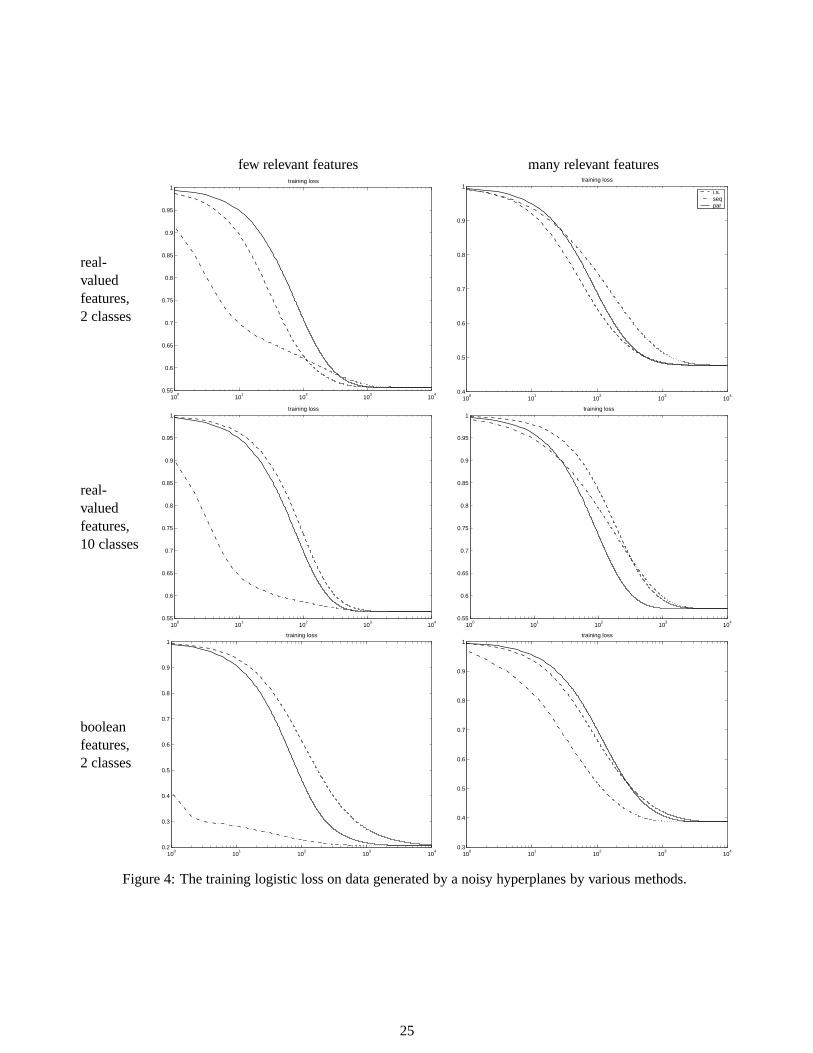
few relevant features many relevant features
real-valuedfeatures,2 classes
100
101
102
103
104
0.55
0.6
0.65
0.7
0.75
0.8
0.85
0.9
0.95
1training loss
100
101
102
103
104
0.4
0.5
0.6
0.7
0.8
0.9
1training loss
i.s.seq par
real-valuedfeatures,10 classes
100
101
102
103
104
0.55
0.6
0.65
0.7
0.75
0.8
0.85
0.9
0.95
1training loss
100
101
102
103
104
0.55
0.6
0.65
0.7
0.75
0.8
0.85
0.9
0.95
1training loss
booleanfeatures,2 classes
100
101
102
103
104
0.2
0.3
0.4
0.5
0.6
0.7
0.8
0.9
1training loss
100
101
102
103
104
0.3
0.4
0.5
0.6
0.7
0.8
0.9
1training loss
Figure 4: The training logistic loss on data generated by a noisy hyperplanes by various methods.
25
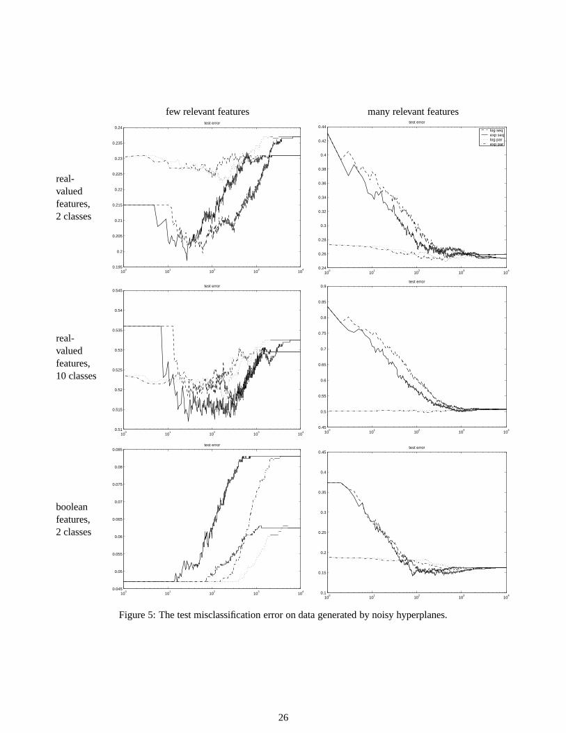
few relevant features many relevant features
real-valuedfeatures,2 classes
100
101
102
103
104
0.195
0.2
0.205
0.21
0.215
0.22
0.225
0.23
0.235
0.24test error
100
101
102
103
104
0.24
0.26
0.28
0.3
0.32
0.34
0.36
0.38
0.4
0.42
0.44test error
log seqexp seqlog parexp par
real-valuedfeatures,10 classes
100
101
102
103
104
0.51
0.515
0.52
0.525
0.53
0.535
0.54
0.545test error
100
101
102
103
104
0.45
0.5
0.55
0.6
0.65
0.7
0.75
0.8
0.85
0.9test error
booleanfeatures,2 classes
100
101
102
103
104
0.045
0.05
0.055
0.06
0.065
0.07
0.075
0.08
0.085test error
100
101
102
103
104
0.1
0.15
0.2
0.25
0.3
0.35
0.4
0.45test error
Figure 5: The test misclassification error on data generatedby noisy hyperplanes.
26
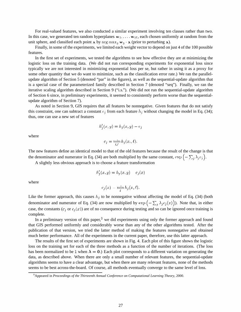
For real-valued features, we also conducted a similar experiment involving ten classes rather than two.In this case, we generated ten random hyperplanesw
1
; : : : ;w
10
, each chosen uniformly at random from theunit sphere, and classified each pointx by argmax
y
w
y
� x (prior to perturbingx).Finally, in some of the experiments, we limited each weight vector to depend on just 4 of the 100 possible
features.In the first set of experiments, we tested the algorithms to see how effective they are at minimizing the
logistic loss on the training data. (We did not run corresponding experiments for exponential loss sincetypically we are not interested in minimizing exponential loss per se, but rather in using it as a proxy forsome other quantity that we do want to minimize, such as the classification error rate.) We ran the parallel-update algorithm of Section 5 (denoted “par” in the figures),as well as the sequential-update algorithm thatis a special case of the parameterized family described in Section 7 (denoted “seq”). Finally, we ran theiterative scaling algorithm described in Section 9 (“i.s.”). (We did not run the sequential-update algorithmof Section 6 since, in preliminary experiments, it seemed toconsistently perform worse than the sequential-update algorithm of Section 7).
As noted in Section 9, GIS requires that all features be nonnegative. Given features that do not satisfythis constraint, one can subtract a constantc
j
from each featurehj
without changing the model in Eq. (34);thus, one can use a new set of features
h
0
j
(x; y) = h
j
(x; y)� c
j
wherec
j
= min
i;`
h
j
(x
i
; `):
The new features define an identical model to that of the old features because the result of the change is thatthe denominator and numerator in Eq. (34) are both multiplied by the same constant,exp
�
�
P
j
�
j
c
j
�
.A slightly less obvious approach is to choose a feature transformation
h
0
j
(x; y) = h
j
(x; y)� c
j
(x)
wherec
j
(x) = min
`
h
j
(x; `):
Like the former approach, this causeshj
to be nonnegative without affecting the model of Eq. (34) (both
denominator and numerator of Eq. (34) are now multiplied byexp
�
�
P
j
�
j
c
j
(x)
�
). Note that, in either
case, the constants (c
j
or cj
(x)) are of no consequence during testing and so can be ignored once training iscomplete.
In a preliminary version of this paper,3 we did experiments using only the former approach and foundthat GIS performed uniformly and considerably worse than any of the other algorithms tested. After thepublication of that version, we tried the latter method of making the features nonnegative and obtainedmuch better performance. All of the experiments in the current paper, therefore, use this latter approach.
The results of the first set of experiments are shown in Fig. 4.Each plot of this figure shows the logisticloss on the training set for each of the three methods as a function of the number of iterations. (The losshas been normalized to be1 when� = 0.) Each plot corresponds to a different variation on generating thedata, as described above. When there are only a small number of relevant features, the sequential-updatealgorithms seems to have a clear advantage, but when there are many relevant features, none of the methodsseems to be best across-the-board. Of course, all methods eventually converge to the same level of loss.
3Appeared inProceedings of the Thirteenth Annual Conference on Computational Learning Theory, 2000.
27
In the second experiment, we tested how effective the new competitors of AdaBoost are at minimizingthe test misclassification error. For this experiment, we used the same parallel- and sequential-update algo-rithms (denoted “par” and “seq”), and in both cases, we used variants based on exponential loss (“exp”) andlogistic loss (“log”).
Fig. 5 shows a plot of the classification error on a separate test set of 2000 examples. When there are fewrelevant features, all of the methods overfit on this data, perhaps because of the high-level of noise. Withmany relevant features, there is not a very large differencein the performance of the exponential and logisticvariants of the algorithms, but the parallel-update variants clearly do much better early on; they seem to “goright to the solution,” exactly the kind of behavior we wouldhope for in such an algorithm.
Acknowledgments
Many thanks to Manfred Warmuth for first teaching us about Bregman distances and for many commentson an earlier draft. John Lafferty was also extraordinarilyhelpful, both in the feedback that he gave us onour results, and in helping us with Theorem 1. Thanks also to Michael Cameron-Jones, Sanjoy Dasgupta,Nigel Duffy, David Helmbold, Raj Iyer and the anonymous reviewers of this paper for helpful discussionsand suggestions. Some of this research was done while Yoram Singer was at AT&T Labs.
References
Berger, A. L., Pietra, S. A. D., & Pietra, V. J. D. (1996). A maximum entropy approach to natural languageprocessing.Computational Linguistics, 22(1), 39–71.
Bregman, L. M. (1967). The relaxation method of finding the common point of convex sets and its appli-cation to the solution of problems in convex programming.U.S.S.R. Computational Mathematics andMathematical Physics, 7(1), 200–217.
Breiman, L. (1997). Arcing the edge. Tech. rep. 486, Statistics Department, University of California atBerkeley.
Breiman, L. (1999). Prediction games and arcing classifiers. Neural Computation, 11(7), 1493–1517.
Censor, Y., & Lent, A. (1981). An iterative row-action method for interval convex programming.Journal ofOptimization Theory and Applications, 34(3), 321–353.
Censor, Y., & Zenios, S. A. (1997).Parallel Optimization: Theory, Algorithms, and Applications. OxfordUniversity Press.
Cesa-Bianchi, N., Krogh, A., & Warmuth, M. K. (1994). Boundson approximate steepest descent forlikelihood maximization in exponential families.IEEE Transactions on Information Theory, 40(4),1215–1220.
Cohen, W. W., & Singer, Y. (1999). A simple, fast, and effective rule learner. InProceedings of the SixteenthNational Conference on Artificial Intelligence.
Csiszar, I. (1995). Generalized projections for non-negative functions.Acta Mathematica Hungarica, 68(1-2), 161–185.
Csiszar, I. (1991). Why least squares and maximum entropy?An axiomatic approach to inference for linearinverse problems.The Annals of Statistics, 19(4), 2032–2066.
28
Darroch, J. N., & Ratcliff, D. (1972). Generalized iterative scaling for log-linear models.The Annals ofMathematical Statistics, 43(5), 1470–1480.
Della Pietra, S., Della Pietra, V., & Lafferty, J. (1997). Inducing features of random fields.IEEE Transac-tions Pattern Analysis and Machine Intelligence, 19(4), 1–13.
Della Pietra, S., Della Pietra, V., & Lafferty, J. (2001). Duality and auxiliary functions for Bregman dis-tances. Tech. rep. CMU-CS-01-109, School of Computer Science, Carnegie Mellon University.
Domingo, C., & Watanabe, O. (2000). Scaling up a boosting-based learner via adaptive sampling. InProceedings of the Fourth Pacific-Asia Conference on Knowledge Discovery and Data Mining.
Duffy, N., & Helmbold, D. (1999). Potential boosters?. InAdvances in Neural Information ProcessingSystems 11.
Freund, Y., & Mason, L. (1999). The alternating decision tree learning algorithm. InMachine Learning:Proceedings of the Sixteenth International Conference, pp. 124–133.
Freund, Y., & Schapire, R. E. (1997). A decision-theoretic generalization of on-line learning and an appli-cation to boosting.Journal of Computer and System Sciences, 55(1), 119–139.
Friedman, J., Hastie, T., & Tibshirani, R. (2000). Additivelogistic regression: A statistical view of boosting.The Annals of Statistics, 38(2), 337–374.
Hoffgen, K.-U., & Simon, H.-U. (1992). Robust trainability of single neurons. InProceedings of the FifthAnnual ACM Workshop on Computational Learning Theory, pp. 428–439.
Kivinen, J., & Warmuth, M. K. (2001). Relative loss bounds for multidimensional regression problems.Machine Learning, 45(3), 301–329.
Kivinen, J., & Warmuth, M. K. (1997). Additive versus exponentiated gradient updates for linear prediction.Information and Computation, 132(1), 1–64.
Kivinen, J., & Warmuth, M. K. (1999). Boosting as entropy projection. InProceedings of the Twelfth AnnualConference on Computational Learning Theory, pp. 134–144.
Lafferty, J. (1999). Additive models, boosting and inference for generalized divergences. InProceedings ofthe Twelfth Annual Conference on Computational Learning Theory, pp. 125–133.
Lafferty, J. D., Pietra, S. D., & Pietra, V. D. (1997). Statistical learning algorithms based on Bregmandistances. InProceedings of the Canadian Workshop on Information Theory.
Littlestone, N., Long, P. M., & Warmuth, M. K. (1995). On-line learning of linear functions.ComputationalComplexity, 5(1), 1–23.
Mason, L., Baxter, J., Bartlett, P., & Frean, M. (1999). Functional gradient techniques for combininghypotheses. In Smola, A. J., Bartlett, P. J., Scholkopf, B., & Schuurmans, D. (Eds.),Advances inLarge Margin Classifiers. MIT Press.
Ratsch, G., Onoda, T., & Muller, K.-R. (2001). Soft margins for AdaBoost. Machine Learning, 42(3),287–320.
Schapire, R. E., & Singer, Y. (1999). Improved boosting algorithms using confidence-rated predictions.Machine Learning, 37(3), 297–336.
29

Schapire, R. E., & Singer, Y. (2000). BoosTexter: A boosting-based system for text categorization.MachineLearning, 39(2/3), 135–168.
Watanabe, O. (1999). From computational learning theory todiscovery science. InProceedings of the 26thInternational Colloquium on Automata, Languages and Programming, pp. 134–148.
30