Embed Size (px)
Citation preview

Logic Regression
Ingo RUCZINSKI Charles KOOPERBERG and Michael LEBLANC
Logic regression is an adaptive regression methodology that attempts to constructpredictors as Boolean combinations of binary covariates In many regression problems amodel is developed that relates the main effects (the predictors or transformations thereof)to the response while interactions are usually kept simple (two- to three-way interactionsat most) Often especially when all predictors are binary the interaction between manypredictors may be what causes the differences in response This issue arises for examplein the analysis of SNP microarray data or in some data mining problems In the proposedmethodology given a set of binary predictors we create new predictors such as ldquoX1 X2 X3 and X4 are truerdquo or ldquoX5 or X6 but not X7 are truerdquo In more speci c terms we try to t regression models of the form g(E[Y ]) = b0 + b1L1 + cent cent cent + bnLn where Lj is anyBoolean expression of the predictors The Lj and bj are estimated simultaneously usinga simulated annealing algorithm This article discusses how to t logic regression modelshow to carry out model selection for these models and gives some examples
Key Words Adaptive model selection Boolean logic Binary variables InteractionsSimulated annealing SNP data
1 INTRODUCTION
In most regression problems a model is developed that only relates the main effects(the predictors or transformations thereof) to the response Although interactions betweenpredictors are sometimesconsideredas well those interactionsare usuallykept simple (two-to three-way interactions at most) But often especially when all predictors are binary theinteraction of many predictors is what causes the differences in response For exampleLucek and Ott (1997) were concerned about analyzing the relationship between diseaseloci and complex traits In the introduction of their article Lucek and Ott recognized theimportance of interactions between loci and potential shortcomings of methods that do nottake those interactions appropriately into account
Ingo Ruczinski is Assistant Professor Department of Biostatistics Bloomberg School of Public Health JohnsHopkinsUniversity 615 N Wolfe Street Baltimore MD 21205-2179(E-mail ingojhuedu)Charles Kooperbergand Michael LeBlanc are Members Fred Hutchinson Cancer Research Center Divisionof Public Health SciencesPO Box 19024 Seattle WA 98109-1024 (E-mail clkfhcrcorg and mikelcraborg)
creg 2003 American Statistical Association Institute of Mathematical Statisticsand Interface Foundation of North America
Journal of Computational and Graphical Statistics Volume 12 Number 3 Pages 475ndash511DOI 1011981061860032238
475
476 I RUCZINSKI C KOOPERBERG AND M LEBLANC
Current methods for analyzing complex traits include analyzing and localizing disease loci oneat a time However complex traits can be caused by the interaction of many loci each withvarying effect
The authorsstated that although nding those interactionsis themostdesirable solutionto the problem it seems to be infeasible
patterns of interactions between several loci for example disease phenotype caused bylocus A and locus B or A but not B or A and (B or C) clearly make identi cation of theinvolved loci more dif cult While the simultaneous analysis of every single two-way pair ofmarkers can be feasible it becomes overwhelmingly computationally burdensome to analyzeall 3-way 4-way to N-way ldquoandrdquo patterns ldquoorrdquo patterns and combinations of loci
The above is an example of the typesof problemswe are concernedaboutGiven a set ofbinary (true and false 0 and 1 on and off yes and no ) predictorsX we try to create newbetter predictors for the response by considering combinations of those binary predictorsFor example if the response is binary as well (which is not a requirement for the methoddiscussed in this article) we attempt to nd decision rules such as ldquoif X1 X2 X3 and X4
are truerdquo or ldquoX5 or X6 but not X7 are truerdquo then the response is more likely to be in class0 In other words we try to nd Boolean statements involving the binary predictors thatenhance the prediction for the response In the near future one such example could arisefrom SNP microarray data (see Daly et al 2001 for one possible application) where oneis interested in nding an association between variations in DNA sequences and a diseaseoutcome such as cancer This article introduces the methodology we developed to ndsolutions to those kind of problems Given the tight association with Boolean logic wedecided to call this methodology logic regression
There is a wealth of approaches to building binary rules decision trees and decisionrules in the computer science machine learning and to a lesser extent statistics literatureThroughout this article we provide a literature review that also serves to highlight thedifferences between our methodologyand other methods which we hope will become clearin the following sectionsTo our knowledge logic regression is the only methodologythat issearching for Boolean combinationsof predictors in the entire space of such combinationswhile being completely embedded in a regression framework where the quality of themodels is determinedby the respectiveobjectivefunctionsof the regressionclass In contrastto themethodsdiscussed in the literaturereviewothermodelsmdashsuch as theCoxproportionalhazards modelmdashcan also be used for logic regression as long as a scoring function can bede ned Making it computationally feasible to search through the entire space of modelswithout compromising the desire for optimalitywe think that logic regression models suchas Y = shy 0 + shy 1 pound [X1 and (X2 or X3)] + shy 2 pound [X1 or (X4 or Xc
5 )] might be able to lla void in the regression and classi cation methodology Section 2 introduces the basics oflogic regression Sections 3 (search for best models) and 4 (model selection) explain howwe nd the best models Section 5 illustrates these features in a case study using simulateddata and data from the Cardiovascular Health Study and describes the results obtained byanalyzing some SNP array data used in the 12th Genetic Analysis Workshop The article
LOGIC REGRESSION 477
concludes with a discussion (Section 6) Explanations of some technical details of logicregression have been deferred to the Appendix
2 LOGIC REGRESSION
Before describing in the second part of this section which models we are interested inwe introduce some terminology that we will use throughout this article
21 LOGIC EXPRESSIONS
We want to nd combinations of binary variables that have high predictive power forthe response variable These combinations are Boolean logic expressions such as L =
(X1 ^ X2) _ Xc3 since the predictors are binary any of those combinations of predictors
will be binary as well We assume familiarity with the basic concepts of Boolean logicWe closely follow Peter Wentworthrsquos online tutorial ldquoBoolean Logic and Circuitsrdquo (httpdiablocsruaczafuncbool) which containsa thorough introductionto Booleanalgebra
deg Values The only two values that are used are 0 and 1 (true and false on and off yesand no )
deg Variables Symbols such as X1 X2 X3 are variables they represent any of the twopossible values
deg Operators Operators combine the values and variables There are three differentoperators ^ (AND) _ (OR) c (NOT) Xc is called the conjugate of X
deg Expressions The combination of values and variables with operators results inexpressions For example X1 ^ Xc
2 is a logic (Boolean) expression built from twovariables and two operators
deg Equations An equation assigns a name to an expression For example using L =
X1 ^ Xc2 we can refer to the expression X1 ^ Xc
2 by simply stating L
Using brackets any Boolean expression can be generated by iteratively combining twovariables a variable and a Boolean expression or two Boolean expressions as shown inEquation (21)
(X1 ^ Xc2 ) ^ [(X3 ^ X4) _ (X5 ^ (Xc
3 _ X6))] (21)
Equation (21) can be read as an ldquoandrdquo statement generated from the Boolean expres-sions X1 ^ Xc
2 and (X3 ^ X4) _ (X5 ^ (Xc3 _ X6)) The latter can be understood as an
ldquoorrdquo statement generated from the Boolean expressions X3 ^ X4 and X5 ^ (Xc3 _ X6)
and so on Using the above interpretation of Boolean expressions enables us to representany Boolean expression in a binary tree format as shown in Figure 1 The evaluation ofsuch a tree as a logic statement for a particular case occurs in a ldquobottom-uprdquo fashion viarecursive substitution The prediction of the tree is whatever value appears in the root (seethe de nition below) after this procedure
478 I RUCZINSKI C KOOPERBERG AND M LEBLANC
3 6
3 4 5 or
1 2 and and
and or
and
Figure 1 The logic tree representing the Boolean expression (X1 ^ Xc2 ) ^ [(X3 ^ X4) _ (X5 ^ (Xc
3 _ X6))]For simplicity only the index of the variable is shown White letters on black background denote the conjugate ofthe variable
We use the following terminology and rules for logic trees [similar to the terminologyused by Breiman Friedman Olshen and Stone (1984) for decision trees]
deg The location for each element (variable conjugate variable operators ^ and _) inthe tree is a knot
deg Each knot has either zero or two subknotsdeg The two subknots of a knot are called its children the knot itself is called the parent
of the subknots The subknots are each otherrsquos siblingsdeg The knot that does not have a parent is called the rootdeg The knots that do not have children are called leavesdeg Leaves can only be occupied by letters or conjugate letters (predictors) all other
knots are operators (_rsquos ^rsquos)
Note that since the representation of a Boolean expression is not unique neither is therepresentation as a logic tree For example the Boolean expression in Equation (21) canalso be written as
[(X1 ^ Xc2 ) ^ (X3 ^ X4)] _ [(X1 ^ Xc
2 ) ^ (X5 ^ (Xc3 _ X6))]
Using the method described above to construct a logic tree from Boolean expressions theresult is a logic tree that looks more complex but is equivalent to the tree in Figure 1 in thesense that both trees yield the same results for any set of predictors See Ruczinski (2000)for a discussion of simpli cation of Boolean expressions in the context of logic regression
In the above we described standard Boolean expressions and introduced logic treesas a way to represent those Boolean expressions conveniently because they simplify theimplementationof the algorithm discussed in Section 3 Appendix A discusses the relationof those trees and other well-known constructsmdashfor example to Boolean expressions in
LOGIC REGRESSION 479
disjunctivenormal formmdashthat play a key role in many publicationsin the computer scienceand engineering literature (see eg Fleisher Tavel and Yeager 1983) and to decision treesas introduced by Breiman et al (1984) (see also Section 23)
22 LOGIC REGRESSION MODELS
Let X1 Xk be binary predictors and let Y be a response variable In this articlewe try to t regression models of the form
g(E[Y ]) = shy 0 +
t
j = 1
shy jLj (22)
where Lj is a Boolean expression of the predictors Xi such as Lj = (X2 _ Xc4 ) ^ X7 We
refer to those models as logic models The above framework includes for example linearregression (g(E[Y ]) = E[Y ]) and logistic regression (g(E[Y ]) = log(E[Y ]=(1 iexcl E [Y ])))For every model type we de ne a score function that re ects the ldquoqualityrdquo of the modelunder consideration For example for linear regression the score could be the residualsum of squares and for logistic regression the score could be the binomial deviance Wetry to nd the Boolean expressions in (22) that minimize the scoring function associatedwith this model type estimating the parameters shy j simultaneously with the search for theBoolean expressions Lj In principle other models such as classi cation models or the Coxproportional hazards model can be implemented as well as long as a scoring function canbe de ned We will come back to this in Section 6
23 OTHER APPROACHES TO MODELING BINARY DATA
There are a large number of approaches to regression and classi cation problems inthe machine learning computer science and statistics literature that are (sometimes) ap-propriate when many of the predictor variables are binary This section discusses a numberof those approaches Boolean functions have played a key role in the machine learning andengineering literature in the past years with an emphasis on Boolean terms in disjunctivenormal form (eg Fleisher Tavel and Yeager 1983MichalskiMozetic Hong and Lavrac1986 Apte and Weiss 1997 Hong 1997 Deshpande and Triantaphyllou 1998) Especiallyin the machine learning literature the methods and algorithms using Boolean functions aregenerally based on either decision trees or decision rules Among the former are some ofthe well-known algorithms by Quinlan such as ID3 (Quinlan 1986) M5 (Quinlan 1992)and C45 (Quinlan 1993) CART (Breiman et al 1984) and SLIQ (Mehta Agrawal andRissanen 1996) also belong to that category The rule-based methods include the AQ family(Michalski et al 1986) the CN2 algorithm (Clark and Niblett 1989) the SWAP1 algo-rithms (Weiss and Indurkhya 1993ab 1995) RIPPER and SLIPPER (Cohen 1995 Cohenand Singer 1999) the system R2 (Torgo 1995Torgo and Gama 1996) GRASP (Deshpandeand Triantaphyllou 1998) and CWS (Domingos 1996) Other approaches to nding opti-mal association rules have been recently proposed for the knowledge discovery and data
480 I RUCZINSKI C KOOPERBERG AND M LEBLANC
mining community by Bayardo and Agrawal (1999) and Webb (2000 2001) Some authorsproposed to combine some of the simpler existing rule-based models into more complexclassi ers (Liu Hsu Ma 1998 Meretakis and Wuthrich 1999) Also mentioned should bethe very nice review article by Apte and Weiss (1997) which describes the use of decisiontrees and rule induction for some data mining examples
Within each of those two categories (trees versus rules) the methods differ by the aimclassi cationversus regression (CART and MARS are exceptionswhich work in bothclassi- cation and regression settings) The vast majority of algorithms published in the literatureare concerned only with classi cation Among the previously mentioned are ID3 C45CN2 SLIQ RIPPERSLIPPER and SWAP1 A myriad of other algorithms or derivationsof the former methods exist for a variety of applications see for example Apte Damerauand Weiss (1994) Weiss and Indurkhya (1993b) introduced an extension to their SWAP1algorithm that learns regression rules in the form of ordered disjunctivenormal form (DNF)decision rules SWAP1R deals with regression by transforming it into a classi cation prob-lem Torgo and Gama (1996) extended this idea by proposing a processor that works onalmost every classi cation method to be used in a regression framework Methods that donot transform regression into classi cation are R2 which searches for logical conditionsin IF THEN format to build piece-wise regression models and M5 which constructs tree-based piece-wise linear models These models trees with linear regression components inthe terminal nodes are known in the statistical literature as treed models (Chipman Georgeand McCulloch 2002) The commercial package CUBIST developed by Quinlan learns IFTHEN rules with linear models in the conclusion An example of such a CUBIST rule isldquoIF (x1 gt 5) amp (x2 lt 3) THEN y = 1 + 2x1 iexcl 8x3 + x5rdquo There is a similarity betweenthis algorithm and the tree-based algorithm M5 which has linear functional models in theterminal nodes
Another noteworthy difference in objectivesacross the methods is the desired format ofthe solutions and in particular their interpretabilityAlthough some authors strongly arguefor compact easily interpretable rules (eg Clark and Niblett 1989 Quinlan 1993 Weissand Indurkhya 1995 Cohen 1995) others emphasize that they care about accuracy andpredictive power the most This is in particular the case when Boolean neural networks arethe method of choice to nd logic rules (Gray and Michel 1992 Thimm and Fiesler 1996Lucek and Ott 1997 Anthony 2001) A nice review article by Wnek and Michalski (1994)compares a decision tree learning method (C45) a rule-learning method (AQ15) a neuralnet trained by a backpropagation algorithm (BpNet) and a classi er system using a geneticalgorithm (CFS) with respect to their predictive accuracy and simplicity of solutions
Multivariateadaptive regression splines (MARS Friedman 1991) is not a methodologyintended for binary predictors but rather a regression methodology to automatically detectinteractions between smooth nonlinear spline-transformed continuouspredictors Becauseof its high amount of adaptivity we will see in Section 51 that even for classi cationproblems with binary predictors a problem that MARS was not designed for it can stillproduce quite reasonable results
LOGIC REGRESSION 481
Possible Moves
4 3
1 or
and
Alternate Leaf
(a)
2 3
1 or
or
Alternate Operator
(b)
2 3
5 or
1 and
and
Grow Branch
(c)
2 3
1 or
and
Initial Tree
2 3
or
Prune Branch
(d)
3 6
2 and
1 or
and
Split Leaf
(e)
1 2
and
Delete Leaf
(f)
Figure 2 Permissible moves in the tree-growing process The starting tree is in the panel in the lower left themoves are illustrated in the panels (a)ndash(f) As in the previous gure only the index of the variable is shown andwhite letters on black background denote the conjugate of a variable
3 SEARCH FOR BEST MODELS
The number of logic trees we can construct for a given set of predictors is huge andthere is no straightforward way to enlist all logic trees that yield different predictions Itis thus impossible to carry out an exhaustive evaluation of all different logic trees Insteadwe use simulated annealing a stochastic search algorithm (discussed in Section 33) Wealso implemented a greedy search algorithm which together with an example is shown inSection 32 But rst we introduce the move set used in both search algorithms
31 MOVING IN THE SEARCH SPACE
We de ne the neighbors of a logic tree to be those trees that can be reached from thislogic tree by a single ldquomoverdquo We stress that each move has a counter move (ie a move topotentiallyget back from the new tree to the old tree) which is important for the underlyingMarkov chain theory in simulated annealingdiscussed later We allow the followingmoves
deg Alternating a leaf We pick a leaf and replace it with another leaf at this positionFor example in Figure 2(a) the leaf X2 from the initial tree has been replaced with
482 I RUCZINSKI C KOOPERBERG AND M LEBLANC
the leaf Xc4 To avoid tautologies if the sibling of a leaf is a leaf as well the leaf
cannot be replaced with its sibling or the complement of the sibling It is clear thatthe counter move to alternating a leaf is by changing the replaced leaf back to whatit was before the move (ie alternating the leaf again)
deg Changingoperators Any ^ can be replacedby a _ and viceversa (eg the operatorat the root in the initial tree in Figure 2 has been changed in Figure 2(b)) These twomoves complement each other as move and counter move
deg Growing and pruning At any knot that is not a leaf we allow a new branch to growThis is done by declaring the subtree starting at this knot to be the right side branchof the new subtree at this position and the left side branch to be a leaf representingany predictor These two side trees are connected by a ^ or _ at the location of theknot For example in the initial tree in Figure 2 we grew a branch in the knot that theldquoorrdquo occupied (panel (c)) The counter move to growing is called pruning A leaf istrimmed from the existing tree and the subtree starting at the sibling of the trimmedleaf is ldquoshiftedrdquo up to start at the parent of the trimmed leaf This is illustrated inFigure 2(d) where the initial tree has been pruned at the ldquoandrdquo
deg Splitting and deleting Any leaf can be split by creating a sibling and determininga parent for those two leaves For example in Figure 2(e) the leaf X3 from the initialtree in Figure 2 has been split with leaf Xc
6 as its new sibling The counter moveis to delete a leaf in a pair of siblings that are both leaves illustrated in Figure 2(f)where X3 has been deleted from the initial tree
Given this move set a logic tree can be reached from any other logic tree in a nitenumber of moves referred to irreducibility in Markov chain theory This is true even if onefor example omits some moves such as pruning and growing In this sense these movesare not absolutely necessary in the move set But inclusion of those additional moves inthe move set enhances the performance of the search algorithm Section 4 discusses how tochoose the optimal model from all candidates For now we simply consider the maximumnumber of trees xed But note that if a model does not have the maximum of trees alloweda permissible move is to add another tree with a single leaf Vice versa if a model has atree with a single leaf a permissible move is to delete this tree from the model
32 GREEDY SEARCH
Similar to the search algorithm in CART (Breiman et al 1984) a greedy algorithm canbe used to search for ldquogoodrdquo logic models In the context of logic regression the rst step isto nd the variable that used as a single predictor minimizes the scoring function (withoutloss of generalization lower scores are better) After this predictor is found its neighbors(states that can be reached by a single move from the given state) are investigated and thenew state is chosen as the state that
1 has a better score than the original state and2 has the best score among the considered neighbors
LOGIC REGRESSION 483
If such a state does not exist the greedy algorithmstops otherwise the neighborsof the newstate are examined and the next state is chosen according to the above described criterionThere is no guarantee that this algorithm nds the best scoring state possible This doeshappen if the search gets ldquostuckrdquo for example if a better tree can be reached in two movesbut not in one move Another potential problem is that in the presence of noise in the datait can happen that even though the tree representing the correct underlying model has beenreached in the search there exist one or more additional moves that improve the score andhence the nal model over- ts the data In contrast to the greedy search for CART a greedymove for logic trees might actually result in a tree of lower or equal complexity (eg bydeleting a leaf or changing an operator respectively)
As an example Figure 3 shows parts of the outcome of a greedy search for a logic treein a classi cation problem on a simulated dataset The data were generated by simulating20 binary predictors with a total of 1000 cases each with each value of each predictorbeing an independent sample from a Bernoulli random variable with probability 1=2 Theunderlying Boolean equation was chosen to be
L = X1 ^ (Xc2 _ X3) ^ [X4 _ (Xc
5 ^ (X6 _ X7))] (31)
For a certain case i where the Boolean equation L was true the response Yi was sampledfrom a Bernoulli random variable with probability 2=3 otherwise it was sampled from aBernoulli random variable with probability 1=3 The score in the greedy search was chosento be the number of misclassi ed cases (ie how often a proposed tree predicted the wrongresponse)
The best single predictor turned out to be predictor X1 having a misclassi cationrate of 434 (434 out of 1000 cases) The second step was splitting the rst leaf intoX1 ^ X3 reducing the misclassi cation rate to 387 After seven steps the correct treewas visited (lower left panel in Figure 3) The true misclassi cation rate in this example is331 However the algorithm did not stop There were possible moves from this tree thatimproved the score the best being splitting leaf X4 into X4 ^ X12 which resulted in a treehaving ve fewer misclassi cations than the tree representing the true Boolean expressionAfter that the greedy algorithm took four more steps (not displayed as trees in Figure 3)until it stoppedyieldinga low misclassi cation rate of 314 These misclassi cation ratesare displayed in the lower right panel in Figure 3 as solid squares The true misclassi cationrates for the respective trees were calculated using model (31) and displayed in the panelas open squares Through tree number seven (which represents the true underlyingBooleanexpression) the true misclassi cation rate is decreasing with the tree number in the greedysearch After that however the following trees also t noise and the true misclassi cationrate increases as expectedThis emphasizes the need for statistical tools for model selectionsince in real-life problems the truth is unknown and the subject of the search The emphasisin this article is on model selection using simulated annealing as discussed in the nextsection However we also developed randomization tests similar to those described inSection 43 for simulated annealing for the greedy search See Ruczinski (2000) for detailsof these tests
484 I RUCZINSKI C KOOPERBERG AND M LEBLANC
4341 387
1 3
and 370
1 3
and 4
and
357
3 2
1 or
and 4
and 346
3 2
1 or 4 5
and or
and 336
3 2 5 6
1 or 4 and
and or
and
331
6 7
3 2 5 or
1 or 4 and
and or
and 326
6 7
3 2 4 12 5 or
1 or and and
and or
and
tree number
mis
cla
ssifi
catio
n ra
te [
]
1 2 3 4 5 6 7 8 9 10 11 12
32
34
363
84
042
Figure 3 The sequence of the rst eight trees visited in the greedy search The number in the upper right corneris the percentage of misclassi ed observations in the simulated data (1000 cases) using the respective tree aspredictor The panel on the lower right shows those mis-classi cation rates (solid squares) together with the truemisclassi cation rates calculated from model (31) (open squares)
Unlike in the above example it is possible that the correct tree is not visited at allThis can happen when the search gets stuck or as shown below if an incorrect variable getschosen This happens frequently particularlywhen some of the predictors are correlated Toshow this we generated a dataset exactly as above except this time we substituted variableX8 (not in the model) by a surrogate of X3 _ X4 For every case i we chose X i
8 to be aBernoulli random variable with probability 09 if Xi
3 _ X i4 was true and Bernoulli with
probability 01 otherwise The outcome of the search is displayed in Figure 4 Now in thethe second step the variable X8 is selected and remains in the model until the very endThe true misclassi cation rate takes a big dip in Step 2 and the resulting tree is basically asurrogate for (X1 ^ (X3 _ X4)) which is a better tree than any other tree with two leaves
33 SEARCH VIA SIMULATED ANNEALING
The simulated annealingalgorithm and its statisticalproperties are discussed in numer-ous publications such as the books by Otten and van Ginneken (1989) and van Laarhovenand Aarts (1987) Below we brie y outline the basics of simulated annealing and describehow we use it to nd good-scoring logic models
LOGIC REGRESSION 485
4341 377
1 8
and 376
8 2
1 or
and
362
2 4
8 and
1 or
and 358
8 7 2 4
and and
1 or
and 353
2 3
8 7 or 4
and and
1 or
and
346
2 3 4 5
8 7 or or
and and
1 or
and
tree number
mis
cla
ssifi
catio
n ra
te [
]
2 4 6 8 10 12
32
34
36
384
042
Figure 4 The sequence of the rst seven trees visited in the greedy search on the data in which the predictors arenot independent Again the number in the upper right corner is the percentage of misclassi ed observations inthe simulated data (1000 cases) using the respective tree as predictor The panel on the lower right shows thosemisclassi cation rates (solid squares) together with the true misclassi cation rates calculated from the correctmodel (open squares)
The annealingalgorithmis de ned on a state space S which is a collectionof individualstates Each of these states represents a con guration of the problem under investigationThe states are related by a neighborhood system and the set of neighbor pairs in S de nesa substructure M in S pound S The elements in M are called moves Two states s s0 are calledadjacent if they can be reached by a single move (ie (s s0) 2 M ) Similarly (s s0) 2 M k
are said to be connected via a set of k moves In all our applications the state space is niteThe basic idea of the annealing algorithm is the following given a certain state pick a
move according to a selection scheme from the set of permissible moves which leads to anew state Compare the scores of the old and the new state If the score of the new state isbetter than the score of the old state accept the move If the score of the new state is not betterthan the score of the old state accept the move with a certain probability The acceptanceprobability depends on the score of the two states under consideration and a parameter thatre ects at which point in time the annealing chain is (this parameter is usually referred to asthe temperature) For any pair of scores the further ahead we are in the annealing schemethe lower the acceptance probability if the proposed state has a score worse than the scoreof the old state This algorithm generally leads to good-scoring states see Otten and van
486 I RUCZINSKI C KOOPERBERG AND M LEBLANC
Ginneken (1989) and van Laarhoven and Aarts (1987)There are various options how to implement the annealing algorithm and t the logic
modelsWe t all trees in the model simultaneouslyThis requires for computationalreasonsthat we preselect the maximum number t of trees which can be chosen arbitrarily large(hardware permitting) which is a conservative choice if we have no a priori idea of howmany trees we maximally want to t If t larger than necessary and the model can betrimmed down if needed In Section 4 this will be discussed in detail For now we assumethat t is known and xed
We usually select one tree in the current logicmodel and then randomly pick (followinga predetermined distribution)a move from the move set for this tree We re t the parametersfor the new model and determine its score which we then compare to the score of theprevious state (logic model) as described above More details about simulated annealingin general and our implementation in particular is given in Appendix B
34 FITTING OTHER MODELS WITH BINARY DATA
The methods discussed in Section 23 can further be distinguishedby their mechanismthat guides the search to nd solutions In general scalability is one of if not the highestpriority in analyzing data to nd Boolean functions that have predictive power Especiallyin data mining problems fast and ef cient search algorithms are crucial Therefore greedytype algorithms similar to the one discussed in Section 32 are standard and often givesatisfactory results (Murthy and Salzberg 1995) In recent years other search methods havegained popularity As is the case for logic regression greedy algorithms do not necessarily nd a global optimum and it has been recognized that alternatives should be consideredif their computational expense is not prohibitive Among those alternatives proposed aregenetic algorithms (Vafaie and DeJong 1991 Bala DeJong Pachowicz 1991 Giordanaand Saitta 1993 Wnek and Michalski 1994) Simulated Annealing (Fleisher et al 1985Sutton 1991 Lutsko and Kuijpers 1994) and a thermal training procedure that is somewhatsimilar to simulated annealing (Frean 1990) The recent statistics literature has seen awealth of alternatives to straight greedy tree searches Buntine (1992) proposed a Bayesianapproach as a stochastic search tool for classi cation trees and Chipman George andMcCulloch (1998) and Denison Mallick and Smith (1998) published Bayesian algorithmsfor CART trees Other approaches were proposed using the EM algorithm (Jordan andJacobs 1994) bootstrapping based techniques such as bagging (Breiman 1996) bumping(Tibshirani and Knight 1999) and iterative reweighting schemes such as boosting (Freundand Schapire 1996) and randomized decision trees (Amit and Geman 1997 Dietterich1999) Comparisons of some of those methods were for example carried out by Quinlan(1996) Dietterich (1999) and Breiman (1999) Another alternative to greedy searches isthe ldquopatientrdquo rule induction method (PRIM) used by Friedman and Fisher (1999)
4 MODEL SELECTION
Using simulated annealing gives us a good chance to nd a model that has the best or
LOGIC REGRESSION 487
close to best possible score However in the presence of noise in the data we know thatthis model likely over ts the data This section introduces some model selection tools forthe simulated annealing search algorithm Similar tools for the greedy search are discussedin Ruczinski (2000)
In this article we use the total number of leaves in the logic trees involvedin a model asa measure of model complexity and call it the model size Different measures are certainlypossible and easily implemented but not further discussed in this article The rst partof this section describes how we ensure nding the best models of a given size which isnecessary in certain types of model selectionThe other two parts of this section describe themodel-selection techniqueswe used in the case studies Examples of these model selectiontechniques are found in Section 5 A potential alternative method of model selection is topenalize the score function for the size of the model in the spirit of AIC BIC and GCVOne difference between our models and traditional setups where these measures are used isthat for logic regression more complicatedmodels do not necessarily have more parametersWe plan to investigate such measures in future work
41 MODELS OF FIXED SIZE
In certain situations it is of interest to know the best scoring tree or the best model ofa certain size This is the case for example when cross-validation is used to determine thebest overall model size as we will see below If the simulated annealing run is carried outwith the move set as described in Section 3 the tree or model size changes constantly andwe cannot guarantee that the nal model is of the desired size To determine the best overallmodel of a xed size we prohibitmoves that increase the tree when its desired size has beenreached In other words we can carry out the simulated annealing as before except we donot suggest branchinga tree or splitting a leaf if the tree has already the desired size Strictlyspeaking this guarantees that we nd the best of up to the desired size However smallertree sizes are desirable in general so this is not be a problem In reality the maximum(desired) tree size almost always is reached anyway provided this size is not too largeAn alternative approach would be to alter the move set discussed in Section 31 to includeonly moves that keep the size of the model unchanged (this requires the de nition of somenew moves) However in our experience the altered move set approach is computationallyconsiderably less ef cient both for the programmer (it complicates the code considerably)and for the computer (as the simulated annealing algorithm converges slower) than theapproach described above
42 TRAININGTEST SET AND CROSS-VALIDATION
We can use a trainingand test-set or a cross-validationapproach to determine the size ofthe logic tree model with the best predictive capability When suf cient data are availablewe can use the training settest set approach That is we randomly assign the cases to twogroups with predetermined sizes using one part of the data as the training set and the other
488 I RUCZINSKI C KOOPERBERG AND M LEBLANC
X Y Perm(Y)
permutation
1
0
Figure 5 The setup for the null model randomization test shown for binary response Y In this test we randomlypermute the entire response
part as test set Thus insteadof using the entire data in the model ttingand model evaluationprocess as described above we t models of xed size using the training set and then picka model size by scoring those models using the independent test set When suf cient datafor an independent test set is not available we can use cross-validation instead Assumewe want to assess how well the best model of size k performs in comparison to modelsof different sizes We split the cases of the dataset into m (approximately) equally sizedgroups For each of the m groups of cases (say group i) we proceed as follows removethe cases from group i from the data Find the best scoring model of size k (as describedin Section 3) using only the data from the remaining m iexcl 1 groups and score the cases ingroup i under this model This yields score deg ki The cross-validated (test) score for modelsize k is deg k = (1=m) i deg ki We can then compare the cross-validated scores for modelsof various sizes
43 RANDOMIZATION
We implemented two types of randomization tests The rst one referred to as ldquonullmodel testrdquo is an overall test for signal in the data The second test a generalization of thistest is a test for model size which can be used to determine an optimal model size Thissection introduces the ideas behind those tests
431 Null Model Test A Test for Signal in the Data
For any model class we consider in our methodology (linear regression logistic re-gression etc) we rst nd the best scoring model given the data Then the null hypothesiswe want to test is ldquoThere is no association between the predictors X and the response Y rdquoIf that hypothesis was true then the best model t on the data with the response randomlypermuted as indicated in Figure 5 for a binary Y should yield about the same score asthe best model t on the original data (Y does not have to be binary in general it was
LOGIC REGRESSION 489
X T1 T2 Y Perm(Y)
1
0
1
0
1
0
1
0
1
0
1
0
1
0
permutation
permutation
permutation
permutation
Figure 6 The setup for the sequential randomization test in this test we permute the response within the groupof cases with the same tted values for all existing trees (here T1 and T2)
chosen binary solely to illustrate the randomization technique in Figure 5) We can repeatthis procedure as often as desired and claim the proportion of scores better than the scoreof the best model on the original data as an exact p value indicating evidence against thenull hypothesis
432 A Test to Detect the Optimal Model Size
If the above described test showed the existence of signal in the data we want todetermine the model that best describes the association between predictors and responseAssume that the best-scoring model has score deg curren and size k We also nd the best scoringmodels of sizes 0 throughk To nd out which model size is optimalwe carry out a sequenceof randomization tests The null hypothesis in each test is ldquoThe optimal model has size jthe better score obtainedby models of larger sizes is due to noiserdquo for some j 2 f0 kgAssume the null hypothesis was true and the optimal model size was j with score deg j Wenow ldquoconditionrdquoon this model considering the tted values of the logic model For a modelwith p trees there can be up to 2p tted classes Figure 6 shows the setup for models withtwo trees
We now randomly permute the response within each of those classes The exact samemodel of size j considered best still scores the same (deg j ) but note that other models of sizej potentiallycould now score better We now nd the overall best model (of any size) on therandomizeddata This model will have a score ( deg curren curren
j ) that is at least as goodbut usuallybetterthan deg j If the null hypothesiswas true and the model of size j was indeed optimal then deg curren
would be a sample from the same distribution as deg curren currenj We can estimate this distribution as
closely as desired by repeating this procedure many times On the other hand if the optimalmodel had a size larger than j then the randomizationwould yield on average worse scoresthan deg curren
We carry out a sequence of randomization tests starting with the test using the nullmodel which is exactly the test for signal in the data as described in the previous subsection
490 I RUCZINSKI C KOOPERBERG AND M LEBLANC
We then condition on the best model of size one and generate randomization scores Thenwe condition on the best model of size two and so on In general model selection is nowbest carried out by comparing the successive histograms of randomization scores deg curren curren
j If weneed an automatic rule we pick the smallest model size where a fraction less than p of therandomization scores have scores better than deg curren Typically we choose p about 020 that islarger than 005 as we do not want to exclude any possibly useful association
44 APPROACHES TO MODEL SELECTION FOR OTHER MODELS WITH BINARY DATA
Model selectiondiffers greatly among the methods discussed in Section 23 Especiallyin the early works on Boolean functions it was often assumed that there was no noise in thedata and the authors strived for minimal complete and consistent rules that is the simplestBoolean functions that perfectly classify all examples (eg Michalski et al 1986 Quinlan1986 Hong 1997) In real-life examples this ldquono-noiserdquo assumption usually does not holdand the above methods result in over- ttingTo account for that a variety of algorithmswereproposed Some of those were simply modi cations of previously mentioned algorithmsFor example Clark and Niblett (1989) pointed out that ID3 can easily modi ed and showedthat extensions exist that circumvent this ldquono-noiserdquo assumption and Zhang and Michalski(1989) proposed a method called SG-TRUNC which they implemented into AQ15 andreleased as version AQ16 Cross-validation is also commonly used for model selectionfor example in M5 (Quinlan 1992) and R2 (Torgo and Gama 1996) Some other pruningtechniques are based on the minimum description length principle such as the one usedin SLIQ (Mehta Agrawal Rissanen 1996) or based on cost-complexity consideration forexample used in CART (Breiman et al 1984) More pruning techniques and a comparisonbetween those can be found in Mehta Rissanen and Agrawal (1995)
5 EXAMPLES
51 A SIMULATION STUDY
As discussed in Section 23 there exist many algorithms in the elds of machinelearning computer science and statistics to model binary data In the statistics literaturethe two best-knownadaptivealgorithmsare CART (Breiman et al 1984)which is especiallyuseful for modeling binary predictor data and MARS (Friedman 1991) which was actuallydesigned for continuous predictors but can still be applied to binary data As the type ofmodels considered for each of these approaches is different it is not hard to come up with anexample where logic regression outperforms MARS and CART or vice versa The intent ofthe simulation study in this section is therefore not to show that logic regression is better oras least as good (in some sense) as CART and MARS but rather to provide an example thatshows that there exist situations in which the underlying model is particularly complicated
LOGIC REGRESSION 491
Table 1 The Results for the Classi cation Part of the Simulation Study The results are averages overten runs Logic regression can t the true model using four terms CART needs seven termsand MARS needs two terms The error rate is calculated using the differences between thetrue signal L and the predictions of the classi er L
Method Logic CART MARS
Selection Truth CV Random CV GCV
true model size mdash 40 40 70 20 tted model size mdash 34 39 32 37number of predictors used 4 34 39 21 41number of predictors X1 X4 used 4 33 33 10 29number of predictors X5 X10 used 0 01 06 11 12fraction of times X10 used 0 00 01 09 08error rate relative to truth 00 55 84 237 154
and logic regression outperforms CART and MARS Coming up with reverse exampleswould be straightforward as well One simulation considers an example that is especiallydif cult for CART It was designed in a way that CART tends to choose a wrong initial splitfrom which it can not easily ldquorecoverrdquo The true model is a fairly simple logic regressionrule Although there exists a CART tree that is equivalent to the logic regression rule usedin the model CART does not produce that tree in practice MARS fares better in this studythan CART but not as well as logic regression
We generated ten datasets with 250 cases and 10 binary predictors each Predictors X1
throughX9 had an independentBernoulli(05)distributionLet L = (X1 ^X2)_(X3^X4)Predictor X10 was equal to L with probability 05 and otherwise was a Bernoulli(716)random variable (note that P (L = 1) = 7=16 in our simulation) For each of the tendatasets we generated a response for classi cation and a response for linear regression Forclassi cation the response for each case was sampled from a Bernoulli(07) distributionif L was true and from a Bernoulli(03) distribution otherwise In the regression case themodel was chosen as Y = 5 + 2L + N (0 1) For both classi cation and regression wepicked the best logic model for each of the ten datasets separately using the cross-validationand the randomizationprocedure The best model for CART was chosen by minimizing the10-fold cross-validation estimates of the prediction error The MARS models were chosento minimize the GCV score with penalty = 3 MARS models were restricted to have nomore than fourth order interactions and a maximum model size of 15 terms The results areshown in Tables 1 and 2 We used the S-Plus program tree to run CART and a version ofMARS written by Tibshirani and Hastie available from httpwwwstatsoxacukpub Forclassi cationusingMARS we t a regressionmodel usingbinary response and thresholdedthe tted values at 05 The smallest model that logic regression can t to model L has sizefour the smallest CART model for L is shown in Figure A1 (p 506) and has seven terminalnodes the smallest MARS model for L is shy aX1X2 + shy bX3X4 iexcl shy cX1X2X3X4 whichhas three terms For the classi cation problem MARS can produce the correct tted valueswith the model shy aX1X2 + shy bX3X4 however In Tables 1 and 2 we refer to the number ofterminal nodes for CART models and the number of terms in a MARS model as ldquomodelsizerdquo
For logic regression model selectionusing randomizationyields models of similar size
492 I RUCZINSKI C KOOPERBERG AND M LEBLANC
Table 2 The Results for the Regression Part of the Simulation Study The results are averages overten runs Note Logic regression can t the true model using four terms CART needs seventerms and MARS needs three terms The root mean squared error is calculated using thesquared differences between the true signal 5 + 2L and the predictions of the tted modelshy 0 + shy 1L
Method Logic CART MARS
Selection truth CV Random CV GCV
true model size mdash 40 40 70 30 tted model size mdash 40 40 100 50number of predictors used 4 40 40 54 44number of predictors X1 X4 used 4 40 40 40 39number of predictors X5 X10 used 0 00 00 14 05fraction of times X10 used 0 0 0 10 02root mean squared error
relative to truth 000 007 007 047 034
as cross-validation This is using the automated procedure as described in Section 432with a cut-off of p = 02 When we visually examined plots like Figure 11 in Section52 we sometimes selected different models than the automated procedure and actuallyended up with results for the randomizationprocedure that are better than those using cross-validationCART selects much larger models and often includes the ldquowrongrdquo predictors Ingeneral it is very much tricked by predictor X10 For classi cation MARS often substitutesone of the correct predictors by X10 Although MARS often has the correct predictors in theselected model the model is usually larger than the smallest model that is needed leadingto less interpretable results For the regression part of the simulation study all methodsperform better as the signal was stronger Both logic regression approaches get the correctmodel each time CART still is tricked by X10 MARS actually picks the correct predictorsseven out of ten times but usually with a too-complicatedmodel For the regression part ofthe simulation study CART always ends up with models with considerably more terminalnodes than needed
Tables 1 and 2 also provide the error rate of the tted model relative to the true modelL = (X1^X2)_(X3^X4) for classi cation and 5+2L for regressionover the design points(see table captions) For the classi cation problem we note that logic regression yields errorrates of under 10 while MARS and CART have error rates of 15 and 23 respectivelyThis should be compared with the 30 noise that we added to the truth For the regressionproblem both logic regression approaches always nd the correct model but since there israndom variation in the estimates of the coef cients the root mean squared error (RMSE)relative to the truth is not exactly 0 Again for the regression problem MARS does muchbetter than CART The RMSE for these approaches can be compared to the noise whichhad standard deviation 1
52 THE CARDIOVASCULAR HEALTH STUDY
The CardiovascularHealth Study (CHS) is a study of coronary heart disease and strokein elderly people (Fried et al 1991) Between 1989 and 1990 5201 subjects over the age
LOGIC REGRESSION 493
Table 3 The 23 Regions of the Cardiovascular Health Study Brain Atlas The predictor number willbe used later to display logic trees and to describe linear models we t The counts are thenumber of CHS patients for whom an infarct was diagnosed The letters in the rst columnindicate the standard anatomicalclusters of the above 23 locationsThey are Cerebral Cortex(Cluster A) Cerebellar Cortex (Cluster B) Cerebellar White Matter (Cluster C) Basal Ganglia(Cluster D) Brain Stem (Cluster E) and Cerebral White Matter (Cluster F)
Cluster Predictor Region Counts
A 1 Anterior Cerebral Artery (frontal lobe) 162 Anterior Cerebral Artery (parietal lobe) 43 Middle Cerebral Artery (frontal lobe) 624 Middle Cerebral Artery (parietal lobe) 435 Middle Cerebral Artery (temporal lobe) 646 Posterior Cerebral Artery (parietal lobe) 67 Posterior Cerebral Artery (temporal lobe) 128 Posterior Cerebral Artery (occipital lobe) 31
B 9 Superior Cerebellar Artery 2310 Anterior Inferior Cerebellar Artery 711 Posterior Inferior Cerebellar Artery 53
C 12 Cerebellar White Matter 58
D 13 Caudate 11014 Lentiform Nuclei 60115 Internal Capsule (anterior limb) 15616 Internal Capsule (posterior limb) 7717 Thalamus 236
E 18 Midbrain 1519 Pons 2920 Medulla Oblongata 0
F 21 Watershed (ACA to MCA) 1022 Watershed (MCA to PCA) 1223 Cerebral White Matter 217
of 65 were recruited in four communities in the United States To increase the minorityrepresentation in the study an additional 687 African Americans were recruited between1992 and 1993 During 1992 and 1994 a subset of these patients agreed to undergo anMRI scan Neuroradiologists blinded to the identity and characteristics of those patientsread the images and attempted to identify the presence and locations of infarcts de nedas an area of brain tissue damaged by lack of oxygen due to compromised blood ow For3647 CHS participants MRI detected strokes (infarcts bigger than 3mm) were recordedas entries into a 23 region atlas of the brain Up to ve infarcts were identi ed per subjectand each of those infarcts was present in up to four of the 23 locations (ie a single infarctwas detectable in up to four regions) For every patient the infarcts were recorded as binaryvariables (absentpresent) in 23 regions Table 3 lists the 23 regions of the CHS atlas andthe number of patients with infarcts in those regions For more details on the scanningprocedure see Bryan et al (1994)
One of the goals of the MRI substudy of the CHS is to assess the associations betweenstroke locations and various response variables such as the one resulting from the mini-
494 I RUCZINSKI C KOOPERBERG AND M LEBLANC
mental state examination a screening test for dementia Patients participate in a question-and-answer session and score points for each correct answer The nal score the sum ofall points earned is a number between 0 (no correct answer) and 100 (everything correct)For more details about this test see Teng and Chui (1987) In our analysis we focusedon demonstrating the use of the logic regression methodology In practice maybe only asubset of the predictors should be included in the analysis since for example there arespatial correlations between predictors Using a clustering approach McClelland (2000)reported improvements after adjusting for gender age and so on These variables were notavailable to us when we started analyzing the data and we did not include those into ourmodel Ruczinski (2000) discussed several approaches to include continuous predictors inlogic regression models See also the example on SNP data in Section 53 in which weincluded continuous predictors as additional variables
Most patients scored in the 90s in the mini-mental test and we found that a logarithmictransformation was bene cial after investigatingpotentialmodel violations such as nonnor-mally distributed (skewed) residuals Since the mini-mental score is a number between 0and 100 we de ned the response variable as
Y = log(101 iexcl [mini-mental score])
Usually such a transformation is avoided because it makes the parameter interpretationand their association to the original mini-mental score rather dif cult but since in ourmethodology we only deal with a very small number of classes of patients (see furtheranalysis below) this is of no importance as the few tted values associated with the mini-mental score can simply be listed without causing confusion
The models we investigated were linear models of the form
Y = shy 0 + shy 1 pound IfL1 is trueg + cent cent cent + shy p pound IfLp is trueg + deg
with deg sup1 N (0 frac14 2) and various numbers p of Boolean expressions These models de negroups of patients with similar stroke patterns in the brain atlas within each group anddifferent average scores between groups In the following analysis we used the residualvariance (residual sums of squares divided by the number of cases considered) as scoringfunction
We rst carried out a ldquonull modelrdquo randomization test as described in Section 431 tting only one tree and allowing up to 16 leaves in the tree The null model ttingthe intercept shy 0 with shy 1 = 0 had a score of 07202 Using simulated annealing the bestscoring model we found had a score of 07029 We permuted the response re t the modelrecorded the score and repeated this procedure 1000 times In Figure 7 we compare thescore for the best scoring model [a] the score for the null model [b] and a histogram ofthe scores obtained from the randomization procedure Since all of those randomizationscores are considerably worse than the score [a] we conclude that there is informationin the predictors with discriminatory power for the (transformed) mini-mental score Theresults we got using models with more than one tree were similar
To get a better idea of the effect of varying model sizes we show the training scores
LOGIC REGRESSION 495
010
020
030
0
score0700 0705 0710 0715 0720
a ba deviance of lowest scoring modelb deviance of null model
Figure 7 The residual variance scores of the null model randomization test The scores in the histogram camefrom linear models with a single tree allowing up to 16 leaves
number of leafs
trai
ning
sco
re0
700
070
50
710
071
5
1 2 3 4 5 6 7 8 9 10 11 12
1
1
1
11
11
1 11 1 1
2
2
22
22
22
2 22
3
3
33
33
33 3
3
Figure 8 The training cross-validation scores of the best linear models with various numbers of leaves and treesThe number of trees allowed in the linear model is indicated by the white number super-imposed on the blacksquares
496 I RUCZINSKI C KOOPERBERG AND M LEBLANC
number of leafs
cros
s va
lidat
ed s
core
070
80
710
071
20
714
071
60
718
072
0
1 2 3 4 5 6 7 8 9 10 11 12
1
1
1
1
1
11
1
1
1
1
12
2
2
2
2 2
2
2
2
2
2
3
3
3
33
33
3
3 3
Figure 9 The cross-validation test scores of the linear models with various numbers of leaves and trees Thenumber of trees allowed in the linear model is indicated by the white number super-imposed on the black squares
number of leafs
scor
e0
705
071
00
715
072
0
1 2 3 4 5 6 7 8 9 10 11 12
Complete dataTraining CV dataTest CV data
Figure 10 Comparison of the scores obtainedby model tting on the complete data (open squares) and the scoresobtained from cross-validation (training sets black triangles test sets black squares) allowing only one tree inthe models
LOGIC REGRESSION 497
(averages of all ten training scores from ten-fold cross-validation) of linear models withone two three trees and varying tree sizes in Figure 8 combined Any model in the classof models with up to k trees and n leaves is also in the class of models with up to k + 1trees and n leaves Further any model in the class of models with up to k trees and n leavesis also in the class of models with up to k trees and n + 1 leaves Therefore the resultsare as expected comparing two models with the same number of trees allowed the modelinvolving more leaves has a better (training) score The more trees we allow in the modelthe better the score for a xed number of leaves Allowing a second tree in the linearmodelsseems to have a larger effect in the training scores (relative to the models with only onetree) than the effect of allowing a third tree in addition to the two trees
However larger models do not imply better cross-validation test scores as shownin Figure 9 The cross-validated scores for models with identical number of leaves butdifferent numbers of trees look remarkably similar Regardless whether we allow one twoor three trees the models of size four seem to be favored Since allowing for more thanone tree obviously is not very bene cial with respect to the cross-validation error we pickfor simplicity the model with only one tree and four leaves We should keep in mind that amodel with k trees involves estimating k + 1 parameters Thus a model with three treeswith the same number of leaves as a model with one tree is more complex
We compare the cross-validated trainingand test scores to the scores using the completedata in Figure 10 For all model sizes the scores obtainedusing the complete data are almostthe same as thescores obtainedfrom the cross-validationtrainingdataThis indicatesthat thesame predictors were selected in most models in the cross-validationtrainingdata comparedto the same sized models tted using the complete data As expected the scores from thecross-validation test data are worse than the training scores However the test score for themodel with four leaves is remarkably close to the training scores indicating that the samepredictors were selected in most models of size four using the cross-validationtraining dataThe vast gap between training and test scores for the models of any size other than fourstrongly discourages the selection of those models
Figure 11 shows histograms of the randomization scores after conditioning on variousnumbers of leaves indicated by the number in the upper left corner of each panel Theaveragesof the randomizationscores decrease when we increase themodelsize we conditionon until we condition on the model with four leaves The overall best score for modelswith one tree (indicated by the left vertical bar in the gure) looks like a sample fromthe distribution estimated by the randomization scores after conditioning on four or moreleaves supporting the choice of four leaves in the selected model The model with fourleaves would also be selected by the automated rule with p = 020 described in Section432
Searching for the best linear model with a single tree of size four using the completedata yielded
Y = 196 + 036 pound IfL is trueg (51)
with the logic tree as shown in Figure 12
498 I RUCZINSKI C KOOPERBERG AND M LEBLANC
0
1
2
3
4
5
0698 0700 0702 0704 0706 0708 0710 0712 0714 0716 0718 0720
Figure 11 The residual variance scores of the randomizationtest for model selection Randomization scores wereobtained conditioningon 0 1 2 3 4 and 5 leaves indicated by the number in the upper left corner of each panelThe solid bar on the right in the panels indicates the score of the null model the solid bar more to the left indicatesthe best overall score found using the original (non-randomized)data The dashed bar in each panel indicates thebest score found for models with one tree and the respective size using the original (nonrandomized) data
LOGIC REGRESSION 499
19 4
or 17
12 or
or
Figure 12 The Logic Tree of the selected model in Equation (51) representing the Boolean equation L =
X12 _ X19 _ X4 _ X17
521 Comparison to Other Modeling Approaches
There are 58 patients with an infarct in region 12 29 patients with an infarct in region19 43 patients with an infarct in region 4 and 236 patients with an infarct in region 17These 366 infarcts occurred in 346 different patients thus these four predictors are pairwisealmost exclusive Since the Boolean expression in (51) has only _ operators the abovemodel is very similar to a linear regression model with these four predictors as main effectssummarized in Table 4 (This linear regression model was also found using backwardsstepwise regression The initial model contained all predictors and no interactions) Notethat 036 the parameter estimate for shy 1 in the logic model is almost within the 95con dence region for each region parameter in the linear regression model
Even though the linear model looks very similar to the model in (51) the logic modelclearly has a much simpler interpretation using the Logic Regression methodology wefound two classes of patients that differ in health history and the performance in the mini-mental test Using the tted values from model (51) we can state that the estimated mediantransformed mini-mental score for patientswith infarcts in either region 4 12 17 or 19 was232 compared to 196 for patients who did not have an infarct in any of those regions Thistranslates to a median mini-mental score of 908 for patients with infarcts in either region
Table 4 Summary of the Regular Regression Model that Compares with the Logic Regression Modelfor the Mini Mental Score Data
shy ˆfrac14 t value
Intercept 1961 0015 13398Region 4 0524 0129 406Region 12 0460 0112 409Region 17 0236 0057 417Region 19 0611 0157 389
500 I RUCZINSKI C KOOPERBERG AND M LEBLANC
4 12 17 or 19 compared to a median mini-mental score of 939 for patients that did nothave an infarct in any of those four regions The residual error is almost exactly the same inthese two models However the ldquostandardrdquo linear regression model by using four binarypredictors de nes 24 = 16 possible classes for each patient But there is no patient withthree or four strokes in regions 4 12 17 and 19 Therefore 5 of those 16 classes are emptyThere is also a signi cant difference in the performance in the mini-mental test betweenpatients with no strokes in regions 4 12 17 and 19 and those who do But there is nosigni cant ldquoadditiverdquo effect that is patients with two strokes in regions 4 12 17 and 19did not perform worse than people with one stroke in either of those regions The logicmodel therefore besides being simpler also seems to be more appropriate
The MARS model is very similar to the linear regression model It was chosen tominimize the GCV score with penalty equal 3 The maximum number of terms used inthe model building was set to 15 and only interactions up to degree 4 were permitted Themodel search yielded
Y = 196 + 053X4 + 037X12 + 024X17 + 061X19 + 105(X12 curren X15) (52)
The additional term compared to the linear regression model concerns patients who have astroke in both regions12 and 15 there are only ve patients for which this appliesHoweverthese ve patients indeed performed very poorly on the mini-mental state examinationAlthough this term certainly is within the search space for the logic model it did not showup in the logic model that was selected using cross-validation and randomization becauseit applied only to 5 out of more than 3500 patients The score (residual error) of the MARSmodel is almost identical to the previously discussed models CART returned a model thatused the same variables as the linear and the logic model shown in Figure 13 Only if allof the four variables are zero (ie the patient has no stroke in either of the four regions)a small value (less than 2) is predicted In fact a simple analysis of variance test does notshow a signi cant difference between the four other group means (and if one bundles themone obtains the logic model) So while the model displayed in Figure 13 is a fairly simpleCART tree we feel that the logic model is easier to interpret
53 APPLICATION TO SNP DATA
This section brie y describes an applicationof the logic regression algorithm to geneticSNP data This applicationwas described in detail by Kooperberg RuczinskiLeBlanc andHsu (2001) Single base-pair differences or single nucleotide polymorphisms (SNPs) areone form of natural sequence variation common to all genomes estimated to occur aboutevery 1000 bases on averageSNPs in the coding regioncan lead to aminoacid substitutionsand therefore impact the function of the encoded protein Understanding how these SNPsrelate to a disease outcome helps us understand the genetic contribution to that disease Formany diseases the interactions between SNPs are thought to be particularly important (seethe quote by Lucek and Ott in the introduction) Typically with any one particular SNPonly two out of the four possible nucleotides occur and each cell contains a pair of every
LOGIC REGRESSION 501
X12
X17
X4
X19
2485
2233
2501
25421959
0
0
0
0
1
1
1
1
Figure 13 CART tree for the mini-mental score data
autosome Thus we can think of an SNP as a random variable X taking values 0 1 and2 (eg corresponding to the nucleotide pairs AA ATTA and TT respectively) We canrecode this variable corresponding to a dominant gene as Xd = 1 if X para 1 and Xd = 0 ifX = 0 and as a recessive gene as Xr = 1 if X = 2 and Xr = 0 if X micro 1 This way wegenerate 2p binary predictors out of p SNPs The logic regression algorithm is now wellsuited to relate these binary predictors with a disease outcome
As part of the 12th Genetic Analysis Workshop (Wijsman et al 2001) the workshoporganizers provideda simulatedgenetic dataset These data were simulatedunder the modelof a common disease A total of 50 independent datasets were generated consisting of 23pedigrees with about 1500 individuals each of which 1000 were alive The variablesreported for each living subject included affection status age at onset (if affected) genderage at last exam sequence data on six genes ve quantitative traits and two environmentalvariables We randomly picked one of the 50 datasets as our training set and anotherrandomly chosen dataset as our test set In the sequence data were a total of 694 sites withat least 2 mutations distributed over all six genes We coded those into 2 pound 694 = 1388binary variables In the remainder we identify sites and coding of variables as followsGiDSj refers to site j on gene i using dominant coding that is GiDSj = 1 if atleast one variant allele exist Similarly GiRSj refers to site j on gene i using recessive
502 I RUCZINSKI C KOOPERBERG AND M LEBLANC
coding that is GiRSj = 1 if two variant alleles exist We identify complements by thesuperscript c for example GiDSjc
As our primary response variables we used the affected status We tted a logisticregression model of the form
logit(affected) = shy 0 + shy 1 poundenviron1 + shy 2 poundenviron2 + shy 3 poundgender+K
i = 1
shy i + 3 poundLi (53)
Here gender was coded as 1 for female and 0 for male environj j = 1 2 are the twoenvironmental factors provided and the Li i = 1 K are logic expressions based onthe 1388 predictors that were created from the sequence data
Initially we t models with K = 1 2 3 allowing logic expressions of at most size 8 onthe training data Figure 14 shows the devianceof the various tted logic regression modelsAs very likely the larger models over- t the data we validated the models by computingthe tted deviance for the independent test set These test set results are also shown inFigure 14 The difference between the solid lines and the dotted lines in this gure showsthe amount of adaptivity of the logic regression algorithm From this gure we see that themodels with three logic trees with a combined total of three and six leaves have the lowesttest set deviance As the goal of the investigation was to identify sites that are possibly
linked to the outcome we preferred the larger of these two models In addition when werepeated the experiment on a training set of ve replicates and a test set of 25 replicates themodel with six leaves actually had a slightly lower test set deviance than the model withthree leaves (results not shown) We also carried out a randomization test which con rmedthat the model with six leaves actually tted the data better than a model with three leavesThe trees of the model with six leaves that was tted on the single replicate are presentedin Figure 15 The logistic regression model corresponding to this logic regression model is
logit(affected) = 044 + 0005 pound environ1 iexcl 027 pound environ2
+198 pound gender iexcl 209 pound L1 + 100 pound L2 iexcl 282 pound L3 (54)
All but the second environment variable in this model are statistically signi cantAs the GAW data is simulated data there is a ldquocorrectrdquo solution (although this is not
a logic regression model) The solution which we did not look at until we selected model(54) showed that there was no effect from genes 3 4 and 5 that all the effect of gene1 was from site 557 that all the effect of gene 6 was from site 5782 and that the effectof gene 2 was from various sites of the gene In addition the model showed an interactionbetween genes 1 and 2 while the effect of gene 6 was additive (but on a different scale thanthe logit scale which we used) For all 1000 subjects with sequence data in replicate 25(which we used) site 76 on gene 1 is exactly the opposite of site 557 which was indicatedas the correct site on the solutions (eg a person with v variant alleles on site 76 always has2 iexcl v variant alleles on site 557 in the copy of the data which we used) Similarly the logicregression algorithm identi ed site 5007 on gene 6 which is identical for all 1000 personsto site 5782 the site which was indicated on the solutions We note that the ldquocorrectrdquo siteon gene 1 appears twice in the logic tree model Once as a recessive coding (G1RS557)
LOGIC REGRESSION 503
number of terms
scor
e75
080
085
090
0
1 2 3 4 5 6 7 8
1
11
12
2
22
2 22
3
33
33
3
11
1
1
2
2 22
2 22
3
33
3
33
Figure 14 Training (solid) and test (open) set deviances for Logic Regression models for the affected state Thenumber in the boxes indicate the number of logic trees
and one effectively as a dominant coding (G1RS76c sup2 G1DS557 on this replicate) forsite 557 suggesting that the true model may have been additiveThe three remaining leavesin the model are all part of gene 2 two site close to the ends of the gene and one site in thecenter All three sites on gene two are dominant
In summary the logic regression model identi ed all sites that were related to theaffected status the correct interaction between genes 1 and 2 and identi ed no false posi-tives As described by Witte and Fijal (2001) the logic regression approach was out of tendifferent approaches the only one that identi ed all correct sites and had no false positiveSNPs
6 DISCUSSION
Logic regression is a tool to detect interactions between binary predictors that areassociated with a response variable The strength of logic regression is that it can nd evencomplicated interactions between predictors that may play important roles in applicationareas such as genetics or identifying prognostic factors in medical data Logic regressionconsiders a novel class of models different from more established methodologies suchas CART and MARS Clearly depending on the application area there will be situationswhere any method outperforms other method We see logic regression as an additional toolin the statistical modelersrsquo toolbox
The logic regression models are not restricted to classi cation or linear regression asmany of the existing methodologiesare Any other (regression) model can be considered as
504 I RUCZINSKI C KOOPERBERG AND M LEBLANC
G2DS4137
G2DS13049
G1RS557
L =1
or
and G6DS5007
L =2
G1RS76
G2DS861
orL =3
Figure 15 Fitted Logic Regression model for the affected state data with three trees and six leaves Variables thatare printed white on a black background are the complement of those indicated
long as a scoring function can be determined In our software for logic regression we alsoimplemented the Cox proportional hazards model using partial likelihood as score Simpleclassi cation problems are trivial to implement using for example the (weighted) numberof misclassi cations as score More complicated models also need to be considered whenanalyzing data with family structure which is often the case in genetic data Since familymembers are genetically related and often share the same environment observations are nolonger independent and one has to take those dependencies into account in modeling thecovariance structure As we envision that logic regression will be useful analyzing geneticdata we plan to investigate scoring functions that take familial dependence into account
As the class of models thatwe consider in logic regression can be very large it is criticalto have a good search algorithm We believe that the simulated annealing algorithm that weuse is much more ef cient in nding a good model than standard greedy algorithms In fu-ture work we plan to investigate the use of Markov chain Monte Carlo algorithms to assessuncertainty about the selected models Because of the similarity between simulated an-nealing and McMC computationally (but not conceptually) this should be straightforwardAs is the case for many adaptive regression methodologies straightforward application ofthe logic regression algorithm would likely over- t the data To overcome this we havediscussed a variety of model selection techniques that can be used to select the ldquobestrdquo logicregression model At this point these techniques are computationally fairly expensive (therunning time for nding the best model or the best model of a particular size for the minimental data took about a minute on a current generation Linux machine therefore 10-foldcross-validation where we investigated models of 30 different sizes and the randomiza-tion tests took several hours) Other techniques some of them much less computationallyintense seem to be feasible This includes for example using a likelihood penalized bythe size of the model as score which would require only one run of the search algorithmThis is similar to using quantities such as AIC BIC or GCV in other adaptive regression
LOGIC REGRESSION 505
methodologies We did not discuss this approach as we wanted to restrict the length of thisarticle
The logic regression software is available from bearfhcrcorgsup1ingorlogic The algo-rithm also includesan option to search for models using only conjunctiveor only disjunctiveBoolean expressions This was achieved in a straightforward manner by altering the moveset to only allow one type of operator Future versions will include several approaches toinclude continuous predictors in logic regression models
APPENDIXES
A RELATIONSHIP BETWEEN LOGIC TREES DECISIONTREES (CART) AND BOOLEAN EXPRESSIONS IN
DISJUNCTIVE NORMAL FORM
The disjunctivenormal form (DNF) is a widespread type of notationof logic statementsin the engineeringand computer science literature A DNF is a Boolean expression writtenas _-combinations of ^-terms For example the Boolean expression
(A ^ Bc) ^ [(C ^ D) _ (E ^ (Cc _ F ))]
can be written in disjunctive normal form as
(A ^ Bc ^ C ^ D) _ (A ^ Bc ^ E ^ Cc) _ (A ^ Bc ^ E ^ F )
It can be shown thatBooleanexpressionsand logictrees as well as otherlogicconstructssuch as Boolean expressions in DNF are equivalent in the sense that the classes of logicexpressions they represent are the same That means for example that every Booleanexpression can be represented in DNF and as a logic tree (Ruczinski 2000)
The logic trees introduced in this article may appear to resemble classi cation trees(eg Breiman et al 1984) In every classi cation tree a leaf can be reached by a paththrough the tree making decisions at every knot If the tree is binary these decisions reduceto checking whether or not the condition investigated at a particular knot is true or falseTo reach a certain leaf all conditions C1 C2 Ck along the path have to be satis ed(ie C1 ^ C2 ^ cent cent cent ^ Ck has to be true) In general there are multiple paths that reach a leafthat predicts class 1 Since there are only two outcome classes (0 and 1) the collection ofall paths P1 P2 Pl that reach a leaf predicting 1 is a complete description of the binaryclassi cation tree Therefore the tree predicts class 1 if the Boolean equation
L = P1 _ P2 _ cent cent cent _ Pl
is true where
Pi = C i1 ^ C i
2 ^ cent cent cent ^ Ciki
506 I RUCZINSKI C KOOPERBERG AND M LEBLANC
C
A D
B0 A 1
0 1 0 B
0 1
01
01
01
01
01
01
A B C D
and and
or
(a) a binary classification tree (b) a logic tree
FigureA1 Equivalence of trees the binaryclassi cation tree and the Logic Tree predict exactly the same outcomefor any set of values of A B C D
Hence every binary classi cation tree can immediately be written as a Boolean equation inDNF For example the tree in Figure A1(a) predicts class 1 if the Boolean equation
L = (Cc ^ A ^ B) _ (C ^ Dc ^ A ^ B) _ (C ^ D)
is trueHowever it is not obvious whether every Boolean expression in DNF can directly be
expressed as a classi cation tree The reason for this is that in a classi cation tree the rstknot is part of every path Using De Morganrsquos rules and standard Boolean operations itcan be shown that a classi cation tree can be constructed from every Boolean expressionHowever these classi cation trees often result in awkward looking constructs much morecomplex than the simple logic trees constructed from the Boolean expressionFor examplefor the tree in Figure A1(a) we have
L = (Cc ^ A ^ B) _ (C ^ Dc ^ A ^ B) _ (C ^ D) sup2 (A ^ B) _ (C ^ D) = L0
This means that the classi cation tree in Figure A1(a) corresponds to the simple Booleanexpression (A ^ B) _ (C ^ D) which can be displayed as very simple logic tree as donein Figure A1(b) (which incidentally is also in DNF) We feel that the simplicity of logictrees is one of their big attractions
B PRACTICAL ASPECTS OF SIMULATED ANNEALING
For simulated annealing in addition to the previously described scoring functions andthe move set we have to specify a selection probability for the moves an acceptancefunction and a cooling scheme Further when we implemented the simulated annealing
LOGIC REGRESSION 507
algorithmfor the logic regression methodologysome practical aspects had to be consideredhow to run the search This section lists what we believe are the most important issues
deg At every stage of the algorithm there is a temperature T (see Section 33 and below)Suppose that the current state of the algorithm has score deg old and the new proposedstate has score deg new where smaller scores are better The new state is accepted withprobability p = min 1 exp [ deg old iexcl deg new] =T (note that Markov chain MonteCarlo MetropolisndashHastings can be seen as simulated annealing algorithm whereT remains constant) See Otten and van Ginneken (1989) and van Laarhoven andAarts (1987) for a discussion of this acceptance probability In general the selectionprobability for the moves affects the performance of the annealing algorithm Forlogic regression we found that it is bene cial to give the highest preference to themoves that alternate the leafs Alternating operators can change the prediction ofthe logic tree under consideration considerably and we usually assign those movesa somewhat lower probability
deg There are two fundamentally different ways how to implement a simulated anneal-ing algorithm One way is to slightly decrease the temperature at each step in thealgorithm The other way is to keep the temperature constant for a certain num-ber of iterations and then decrease the temperature by a somewhat larger amountThe performances of both algorithms have been studied (Otten and van Ginneken1989 van Laarhoven and Aarts 1987) and in general one cannot claim that oneway of running the chain is superior to the other However we nd that monitoringthe convergence process is more straightforward using a sequence of homogeneousMarkov chains (runs at constant temperature)
deg In the beginning of a simulated annealing run with high temperatures virtually allproposed moves are accepted Towards the end almost every proposed move isrejected Somewhere in between is the ldquocrunch timerdquo where we want to spend mostof the computing time To speed up the simulated annealing and avoid spendingtoo much time either at the beginning or the end of the run we implemented thefollowing features
ndash Runninga Markov chain at xed temperature we keep track of how many moveshave been accepted If this number reaches a predetermined threshold we exitthe Markov chain (even though the number of iterations speci ed has not beenreached) and lower the temperature to its next value This avoids spending toomuch time at the beginningof the run in ldquorandom modelsrdquo Later in the annealingalgorithm we will not be able to reach this threshold and the Markov chains runfor their full lengths The threshold typically is between 1 and 10 of theprespeci ed number of iterations for a chain at a xed temperature
ndash We have to specify a lowest temperature before starting the simulated annealingrun Several criteria can be considered to exit the simulated annealing run earlywhen the search virtually has been nished for example the case when no moves
508 I RUCZINSKI C KOOPERBERG AND M LEBLANC
were accepted for a substantial number of consecutive chains This avoids run-ning the algorithmall the way to its end althoughno improvementcan be achievedanymore It also allows setting the lowest temperature arbitrarily low since theexit criteria can be chosen independently of the lowest temperature considered
deg To implement a simulated annealing run we have to specify a temperature schemeThat means we have to choose the starting (highest) temperature the nishing(lowest) temperatureand thecoolingschemewhichalsodeterminesthe totalnumberof chains we run at constant temperatures In making this decision there is usuallysome trial and error involved since in practice the cooling scheme depends on thedata we are analyzing The theory of simulated annealing is thoroughly discussedfor example in the books by van Laarhoven and Aarts (1987) and Otten and vanGinneken (1989) stating conditions for the simulated annealing run under whichwe can guarantee to nd an optimal scoring state One obvious problem is thatwe cannot run chains of length in nity as required the optimal state may not bereached in practice We need to make sure that the individual chains we run comeclose to their limiting distributions and cool suf ciently slowly such that this canbe achieved with a reasonable number of iterations in the chain The choices for theparameters we pick therefore in uence each other We already explained above thatpicking the highest and lowest temperature is not a problem We want the startingtemperature high enough such that the rst chains are essentially random walksThis can be controlled by monitoring the acceptance rate The lowest temperature ischosen such that the above described exit criterion terminates the chain Dependingon the size of the dataset we usually choose for the exit criterion the number ofchains without acceptancebetween 10 and 20 The temperatures are usually loweredin equal increments on a log10 scale The number of chains between two subsequentpowers of 10 depend on the data as well usually the number is between 25 and100 This translates to decreasing the temperature between homogeneous chains bya factor between 091 and 098 The lengths of the individualchains for the data welooked at so far have been between 10000 and 100000The search for a single bestmodel usually takes only a few minutes on a Pentium processor the randomizationtests (depending on the number of permutations carried out) usually require severalhours of CPU time
deg Every logic tree has a nite number of neighbors Especially toward the end of therun at low temperatures very few moves get accepted Because simulated annealingis a probabilisticsearch a move mightget rejected several times before it is acceptedThe worst ldquobottle neckrdquo in terms of computing time is the evaluation of the logictrees that is deriving the values of their underlying Boolean equation from theleaves for each case Because the acceptance of a move given the temperature andthe score of the current model depends only on the score of the proposed modelwe implemented a subroutine that keeps track of all states visited and their scoresin a table Therefore for the decision whether or not to accept a certain move froma given state the trees of the proposed model have to be evaluated only once which
LOGIC REGRESSION 509
speeds up the search dramatically at lower temperatures After a move is acceptedthe old table is ushed and a new table is generated
deg In theory trees of any size can be grown but considering that in our applicationswewant to be able to interpret these models it makes sense to limit the tree sizes to areasonable number of leaves We usually limit the number of leaves to a maximumof 8 or 16 per tree As previously noted we also limit the number of trees we allowIn the case studies we carried out optimal logic regression models typically hadbetween one and three logic trees However we usually allow up to ve trees at thebeginning of our search for good models
ACKNOWLEDGMENTSWe thank Richard Kronmal and Robyn McClelland for providing us with the data used in Section 52 and
the permission to use those data in this article We thank the GAW organizers for permission to use their datain this article Ingo Ruczinski and Charles Kooperberg were supported in part by NIH grant CA74841 MichaelLeBlanc was supported by NIH grant CA90998 All authors were supported in part by NIH grant CA53996 TheGAW workshop is supported by NIH grant GM31575
[Received June 2001 Revised September 2002]
REFERENCES
Amit Y and Geman D (1997) ldquoShape Quantization and Recognition with Randomized Treesrdquo Neural Compu-tation 9 1545ndash1588
AnthonyM (2001)ldquoDiscrete Mathematics of Neural Networks Selected TopicsrdquoSIAM Monographson DiscreteMathematics and Applications 8
Apte C Damerau F and Weiss S M (1994) ldquoTowards Language Independent Automated Learning of TextCategorisation Modelsrdquo Research and Development in Information Retrieval 23ndash30
Apte C and Weiss S M (1997) ldquoData Mining with Decision Trees and Decision Rulesrdquo Future GenerationComputer Systems 13 197ndash210
Bala J DeJong K and Pachowicz P (1991) ldquoLearning Noise Tolerant Classi cation Procedures by Integrat-ing Inductive Learning and Genetic Algorithmsrdquo in Proceedings of the First International Workshop onMultistrategy Learning MSL-91 pp 316ndash323
Bayardo R J Jr and Agrawal R (1999) ldquoMining the Most Interesting Rulesrdquo Knowledge Discovery and DataMining 145ndash154
Breiman L (1996) ldquoBagging Predictorsrdquo Machine Learning 24 123ndash140
(1999) ldquoRandom ForestsmdashRandom Featuresrdquo Technical report Department of Statistics University ofCalifornia Berkeley
Breiman L Friedman J H Olshen R A and Stone C J (1984) Classi cationandRegression Trees BelmontCA Wadsworth
Bryan R N Manolio T A Schertz L D Jungreis C Poirier V C Elster A D and Kronmal R A (1994)ldquoA Method for Using MR to Evaluate the Effects of Cardiovascular Disease on the Brain the CardiovascularHealth Studyrdquo American Journal of Neuroradiology 15 1625ndash1633
Buntine W (1992) ldquoLearning Classi cation Treesrdquo Statistics and Computing 2 63ndash73
Chipman H George E and McCulloch R (1998) ldquoBayesian CART Model Searchrdquo (with discussion) Journalof the American Statistical Association 93 935ndash960
(2002) ldquoBayesian Treed Modelsrdquo Machine Learning 48 299ndash320
510 I RUCZINSKI C KOOPERBERG AND M LEBLANC
Clark P and Niblett T (1989) ldquoThe CN2 Induction Algorithmrdquo Machine Learning 3 261ndash283
Cohen W (1995) ldquoFast Effective Rule Inductionrdquo International Conference on Machine Learning 115ndash123
Cohen W and Singer Y (1999) ldquoA Simple Fast and Effective Rule Learnerrdquo in Proceedings of Annual Con-ference of American Association for Arti cial Intelligence 335ndash342
Daly M J Rioux J D Schaffner S F Hudson T J and Lander E S (2001) ldquoHigh Resolution HaplotypeStructure in the Human Genomerdquo Nature Genetics 29 229ndash232
Denison D Mallick B and Smith A F M (1998) ldquoA Bayesian CART Algorithmrdquo Biometrika 85 363ndash377
Deshpande A S and Triantaphyllou E (1998) ldquoA Greedy Randomized Adaptive Search Procedurerdquo Mathe-matical Computer Modelling 27 75ndash99
Dietterich T G (1999)ldquoAn Experimental Comparison of Three Methods for ConstructingEnsembles of DecisionTrees Bagging Boosting and Randomizationrdquo Machine Learning 40 139ndash158
Domingos P (1996) ldquoLinear-Time Rule Inductionrdquo Knowledge Discovery and Data Mining 96ndash101
Fleisher H Tavel M and Yeager J (1983) ldquoExclusive-OR Representations of Boolean Functionsrdquo IBM Journalof Research and Development 27 412ndash416
Fleisher H Giraldi J Martin D B Phoenix R L and Tavel M A (1985) ldquoSimulated Annealing as aTool for Logic Optimization in a CAD Environmentrdquo in Proceedings of the International Conference onComputer-Aided Design pp 203ndash205
Frean M (1990) ldquoSmall Nets and Short Paths Optimising Neural Computationrdquo PhD thesis University ofEdinburghCenter for Cognitive Science
Freund Y and Schapire R (1996) ldquoExperiments With a New Boosting Algorithmrdquo in Proceedings of the 13thInternational Conference on Machine Learning pp 148ndash156
Fried L P Borhani N O Enright P Furberg C D Gardin J M Kronmal R A Kuller L H Manolio TA Mittelmark M B Newman A B OrsquoLeary D H Psaty B Rautaharju P Tracy R P and Weiler PG (1991) ldquoThe Cardiovascular Health Study Design and Rationalerdquo Annals of Epidemiology 1 263ndash276
Friedman J H (1991) ldquoMultivariate Adaptive Regression Splinesrdquo (with discussion) The Annals of Statistics19 1ndash141
Friedman J H and Fisher N I (1999) ldquoBump Hunting in High-Dimensional Datardquo Statistics and Computing9 123ndash162
Giordana A and Saitta L (1993) ldquoREGAL An Integrated System for Learning Relations Using GeneticAlgorithmsrdquo in Proceedings of the Second International Workshop on Multistrategy Learning (MSL-93)pp 234ndash249
Gray D L and Michel A N (1992) ldquoA Training Algorithm for Binary Feedforward Neural Networksrdquo IEEETransactions on Neural Networks 3 176ndash194
Hong S (1997) ldquoR-MINI An Iterative Approach for Generating Minimal Rules from Examplesrdquo IEEE Trans-actions on Knowledge and Data Engineering 9 709ndash717
Hong S Cain R G and Ostapko D L (1974) ldquoMINI A Heuristic Approach for Logic Minimizationrdquo IBMJournal of Research and Development 18 443ndash458
Jordan M I and Jacobs R A (1994) ldquoHierarchical Mixtures of Experts and the EM Algorithmrdquo NeuralComputation 6 181ndash214
Kooperberg C Ruczinski I LeBlanc M L and Hsu L (2001) ldquoSequence Analysis using Logic RegressionrdquoGenetic Epidemiology 21 Supplement 1 626ndash631
Liu B Hsu W and Ma Y (1998) ldquoIntegrating Classi cation and Association Rule Miningrdquo Proceedings ofInternational Conf on Knowledge Discovery and Data Mining pp 80ndash86
Lucek P R and Ott J (1997) ldquoNeural Network Analysis of Complex Traitsrdquo Genetic Epidemiology 14 1101ndash1106
Lutsko J F and Kuijpers B (1994)ldquoSimulated Annealing in the Constructionof Near-Optimal Decision Treesrdquoin Selecting Models from Data AIampStatistics IV New York Springer pp 453ndash462
McClelland R (2000) ldquoRegression Based Variable Clustering for Data Reductionrdquo PhD thesis University ofWashington Department of Biostatistics
Mehta M Rissanen J and Agrawal R (1995) ldquoMDL-Based Decision Tree Pruningrdquo in Proceedings of theFirst International Conference on Knowledge Discovery and Data Mining KDD95 pp 216ndash221
Mehta M Agrawal R and Rissanen J (1996) ldquoSLIQ A Fast Scalable Classi er for Data Miningrdquo ExtendingDatabase Technology 18ndash32
LOGIC REGRESSION 511
Meretakis D and Wuthrich B (1999) ldquoExtending Naive Bayes Classi ers Using Long Itemsetsrdquo KnowledgeDiscovery and Data Mining 165ndash174
Michalski R Mozetic I Hong J and Lavrac N (1986) ldquoThe Multi-Purpose Incremental Learning SystemAQ15 and its Testing Application to Three Medical Domainsrdquo Proceedings of the AAAI pp 1041ndash1045
Murthy S K and Salzberg S (1995) ldquoDecision Tree Induction How Effective is the Greedy HeuristicrdquoKnowledge Discovery and Data Mining 222ndash227
Otten R H and Ginneken L P (1989) The Annealing Algorithm Boston Kluwer Academic Publishers
Quinlan J R (1986) ldquoInduction of Decision Treesrdquo Machine Learning 1 81ndash106
(1992) ldquoLearning with Continuous Classesrdquo 5th Australian Joint Conference on Arti cial Intelligence343ndash348
(1993) C45 Programs for Machine Learning San Mateo CA Morgan Kaufmann
(1996) ldquoBagging Boosting and C45rdquo in Proceedings of AAAIrsquo96 National Conference on Arti cialIntelligence pp 725ndash730
Ruczinski I (2000)ldquoLogic Regression and Statistical Issues Related to the Protein FoldingProblemrdquo PhD thesisUniversity of Washington Department of Statistics
Sutton C (1991) ldquoImproving Classi cation Trees with Simulated Annealingrdquo in Proceedings of the 23rd Sym-posium on the Interface ed E Kazimadas Fairfax VA Interface Foundation of North America
Teng E L and Chui H C (1987) ldquoThe Modi ed Mini-Mental State (3MS) Examinationrdquo Journal of ClinicalPsychiatry 48 314ndash318
Thimm G and Fiesler E (1996) ldquoA Boolean Approach to Construct Neural Networks for Non-Boolean Prob-lemsrdquo Proceedings of the Eighth International Conference on Tools with Arti cial Intelligence (ICTAI) pp458ndash459
Tibshirani R and Knight K (1999) ldquoModel Search and Inference by Bootstrap lsquoBumpingrsquordquo Journal of Com-putational and Graphical Statisticsrsquo 8 671ndash686
Torgo L (1995) ldquoData Fitting with Rule-based Regressionrdquo in Proceedings of the 2nd International Workshopon Arti cial Intelligence Techniques (AITrsquo95) eds J Zizka and P Brazdil Brno Czech Republic
Torgo L and Gama J (1996) ldquoRegression by Classi cationrdquo Brazilian Symposium on Arti cial Intelligence51ndash60
Vafaie H and DeJong K (1991) ldquoImproving the Performance of a Rule Induction System Using GeneticAlgorithmsrdquo in Proceedings of the First International Workshop on Multistrategy Learning MSL-91 pp305ndash315
van Laarhoven P J and Aarts E H (1987) Simulated Annealing Theory and Applications Boston KluwerAcademic Publishers
Webb G (2000) ldquoEf cient Search for Association Rulesrdquo in Proceedings of the sixth International Conferenceon Knowledge Discovery and Data Mining KDD 2000 99ndash107
(2001) ldquoDiscovering Associations with Numeric Variablesrdquo in Proceedings of the seventh InternationalConference on Knowledge Discovery and Data Mining KDD 2001 pp 383ndash388
Weiss S M and Indurkhya N (1993a) ldquoOptimized Rule Inductionrdquo IEEE Expert December 61ndash69
(1993b) ldquoRule-Based Regressionrdquo in Proceedings of the 13th InternationalJoint Conference on Arti cialIntelligence (IJCAI) pp 1072ndash1078
(1995) ldquoRule-Based Machine Learning Methods for Functional Predictionrdquo Journal of Arti cial Intelli-gence Research 3 383ndash403
Wijsman E M Almasy L Amos C I Borecki I Falk C T King T M Martinez M M Meyers DNeuman R Olson J M Rich S Spence M A Thomas D C Vieland V J Witte J S MacCluerJ W (2001) ldquoAnalysis of Complex Genetic Traits Applications to Asthma and Simulated Datardquo GeneticEpidemiology 21 Supplement 1
Witte J S and Fijal B A (2001) ldquoIntroduction Analysis of Sequence Data and Population Structurerdquo GeneticEpidemiology 21 Supplement 1 pp 600ndash601
Wnek J and Michalski R (1994) ldquoComparing Symbolic and Subsymbolic Learning Three Studiesrdquo MachineLearning A MultistrategyApproach eds R Michalski and G Tecuci 4 San Francisco Morgan-Kaufmann
Zhang J and Michalski R S (1989) ldquoRule Optimization via SGndashTrunc Methodrdquo European Working Sessionon Learning 251ndash262
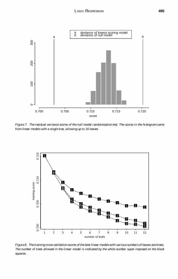
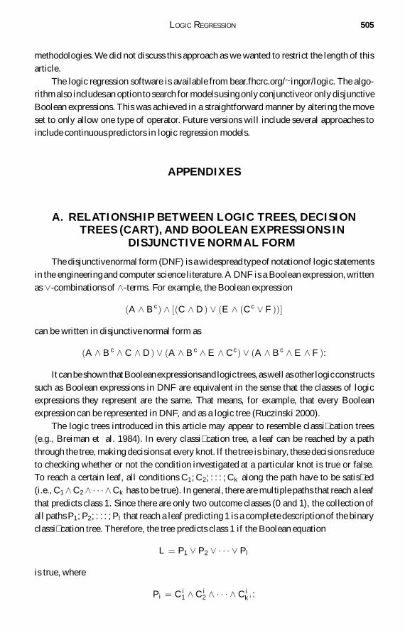


![Regression with Ordered Predictors via Ordinal Smoothing Splines · powerful smoothing spline ANOVA framework [15]—provides an appealing approach for including ordinal predictors](https://img.pdfslide.us/doc/110x75/5f56b73c555d7b2ea3790a9a/regression-with-ordered-predictors-via-ordinal-smoothing-splines-powerful-smoothing.jpg)