Location Dependent Database Access - Lyle School of ...lyle.smu.edu/~mhd/8331sp08/ldd.doc · Web viewIn this paper we provide an introduction into the subject of location dependent

Location-Dependent Database Access

Faïza Najjar Sean Kelley, Margaret H. DunhamNational School of Computer Science Department of Computer Science and Engineering

La Manouba 2010 PO Box 750122Tunisia Dallas, Texas 75275-0122

[email protected] (kelley)[email protected]

Abstract. Database queries stated in a mobile computing environment are significantly impacted by that mobility. In this paper we provide an introduction into the subject of location dependent database access. The coverage is quite broad and is aimed as providing the reader with sufficient content and references to begin research in this area. We include discussions of architecture and an overview of different types of location based mobile queries. A major portion of the paper deals with a detailed examination of nearest-neighbor queries and Voronoi diagrams.

Table of contents

1. Introduction....................................................................................................................................12. Architecture................................................................................................................................83. Overview of Location-Dependent Queries............................................................................114. Overview of Moving Object Queries and Databases............................................................135. Location Modeling and Translation.......................................................................................176. Nearest-neighborQueries Through Point Location and Indexing......................................187. Conclusions...............................................................................................................................27References.....................................................................................................................................28

Najjar, Kelley, Dunham 1

1. IntroductionIn a mobile and wireless environment, efficient and consistent data access is a challenging research area,

because of the weak connectivity and resource constraints. The mobile data access strategies can be

essentially distinguished by delivery modes. The modes for server delivery can be described as client

pull, server-push, or hybrid:

Client pull (sometimes called on-demand access mode): A mobile client first submits a query via

the uplink channel and then “pulls” data, from the server through a wireless network (the

downlink channel), in the same manner as in a traditional client-server system.

The server-push (also called broadcast [15]): The mobile client receives information as a result of

his or her whereabouts without having to actively submitting a query. The information sent to the

mobile client may be either on a public wireless channel (e.g. a welcome message when entering

a new town) or may be a subscription-based (e.g. alert system).

The hybrid delivery integrates both server-push and client pull delivery.

Location-dependent data access assumes that a mobile user queries data where the value is dependent on

his/her location. A typical query of this type is:

“Where is the closest restaurant?”

This query may be stated explicity (in the client pull environment) or implicitly (in the push

environment). In a broadcast setting, a content provider can broadcast restaurant information for a local

area near the broadcast station. A Location Dependent Query (LDQ) is a mobile query where the result of

the query depends on the location of the user making the query [4, 23, 26]. This definition can be

expanded to include a broadcast environment. Here the content of the broadcast is based on the location

of the broadcast station. Thus, as a mobile user roams, the result of his implicit query (that is the data that

he receives) changes.

We conclude this section by reviewing some terms and background commonly used within location-

dependent data and queries in wireless environments. We then briefly overview temporal and spatial

database concepts as these are important to understanding location dependent database access.

Subsequent sections of this chapter examine architectural issues related to location dependent data access,

an overview of location dependent queries, an overview of moving object databases and queries, location

modeling and translation, and nearest neighbor queries and indexing.


11. Terminology

As long as people move across the earth’s surface, the need to know their current location anywhere and

anytime has become a very important constraint in mobile databases. The term location refers to the

position of a point relative to a geometric subdivision or a given set of disjoint geometric objects [1, 16].

Before studying queries and data access approaches in mobile databases, it is important to emphasize

some fundamental properties of location data, such as:

Location models : we distinguish two kinds of location, geometric (or geographic) and. semantic

(or symbolic) locations (see Figure 1):

o The available mechanisms for identifying the geometric location can be divided into two

basic classes :

1. A location is specified, in the World Geodic System 1984 (WGS84), as a three-

dimensional unique location – 3 coordinates (latitude, longitude and altitude). These

coordinates can be easily provided by a satellite-based positioning system (e.g. the

most widely known the Global Positioning System – GPS).

2. A location can also be considered by a set of coordinates defining an area’s bounding

geometric shape (such as polygon).

Geometric location can be considered in heterogeneous systems and it is common used in

outdoor domain [14]. However, mobile users are often interested in the meaning of

location rather than the geometric coordinates.

o Semantic location is the logical representation of the real-world entities describing the

location space. Entities can be cities, street address, zip code, or system-defined elements

such as cell IDs in cellular phone networks, infrared beacons, or WLAN access point IDs

in the indoor domain. The last entities are uniquely identifiable by hierarchical naming

system such as location trees.

Finally, both geometric and symbolic locations are present and have to be considered in LDQ. In

addition, the process of converting a given symbolic location to x, y coordinates (e.g. latitude,

longitude) [22] is called geocoding (see Figure 1). The opposite function of geocoding is reverse

geocoding, which is the process of deriving the semantic location of a specified longitude/latitude

coordinate.


Precision depends on the measurement errors in geometric coordinates and on the completeness

and accuracy of address names (normalized).

Scope is the geometric area of potential coordinates (it often takes the shape of polygon). A valid

scope (also called a data region) of a spatial data was introduced by Zheng et al. [15]; it defines

the region within which the result is valid with respect to the query.

Additional spatial data. Besides the location, more spatial information sometimes is required,

such as orientation or speed.

Figure 1. Location model architecture

The properties of location can affect the processing of queries significantly when the user changes his

(her) position in a mobile and wireless environment.

1.2. Location Dependent Data vs Spatial Data vs Temporal Data

Space and time are two powerful forces that have mesmerized scientists, theologians, astrologists and

philosophers for 2500 years. Einstein’s Theory of General Relativity described the “effect of gravitation

on the shape of space and the flow of time” [11]. Einstein’s work led to the development of what is

referred to as “spacetime”—“a universe in which space and time are woven together into a single fabric”

[11]. The relationship between space and time will be a key theme throughout this survey paper because

this relationship serves as a foundation for queries stated in a mobile computing environment.

The term “Spatio” is derived from the word “spatial” which is defined as “relating to, involving, or

having the nature of space”. A Spatial Database (SDB) “offers spatial data types in its data model and

query language and supports spatial data types in its implementation, providing at least spatial indexing

and spatial join methods”. Spatial data is oftentimes geographic or geometric in nature and the “space of

interest” is dependent upon the problem(s) being solved [10]. The problem space may be, for example,

the surface of Mars (geographic space), the layout for a VLSI design (man made space) or the structure of

a DNA sample taken from an extinct species (sub-atomic space) [10]. Oftentimes, the complexity of the

space being studied can be easier to understand if it is broken down into “large collections of relatively

simple geometric objects” [10]. For example, points, lines and regions (see Figure 2) are oftentimes

found in SDBs and are used to model real-world entities. A line can be used to track movement through

space or create a connection between two or more points (i.e. roads, boundaries, etc). A region can be

two or three-dimensional, may have holes and can consist of many disjoint pieces [10].


Location

Semantic location

GeometricLocatio

nReverse

Geocoding

Geocoding

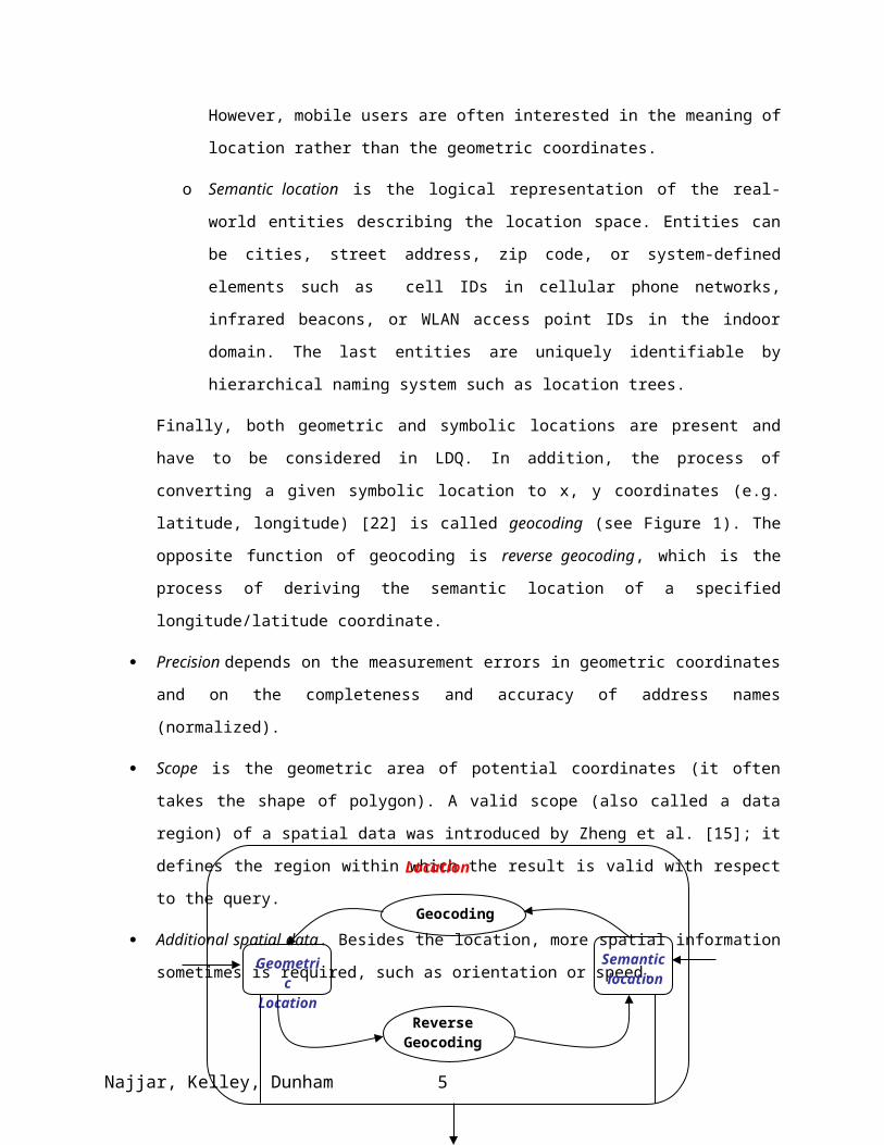
Figure 2. Point, line, region and region with gaps

The position of these objects may be viewed at different levels of granularity, and the geometric

representation of an object may change as the granularity changes. For example, a city may be viewed as

a line or region, depending upon the level of detail required by the model [13]. In addition, spatial objects

oftentimes have descriptive properties that may or may not change depending upon the position of an

object within space. Furthermore, these objects may be associated with one another using spatial

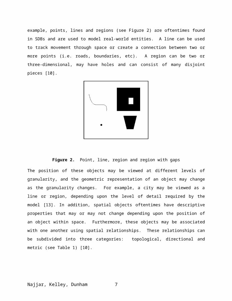
relationships. These relationships can be subdivided into three categories: topological, directional and

metric (see Table 1) [10].


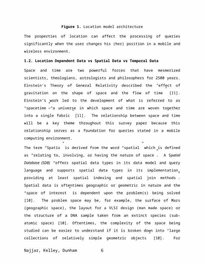
Table 1. Spatial Relationship Types

Relationship

Type

Examples

Topological inside, disjoint, overlaps

Directional above, below, north_of, south_of

Metric distance < 30, distance = 10

A spatial query language would then contain special operators that would facilitate the inspection and

manipulation of these objects. Specifically, one might use the ADJACENT operator to identify two

regions that touch each other. Likewise, it may be necessary to use an ABOVE or BELOW operator to

determine the direction that one point lies in respect to another point. Various index techniques are used

to support the querying of spatial objects in an effort to decrease the access time. Spatial indexes are

composed of keys that allow for a less complex representation of the underlying objects. This, in turn,

decreases the amount of I/O or processing needs for spatial queries.

Temporal databases (TDBs) allow for the “management of time-varying data” [12]. Most applications

are temporal in nature with different degrees of support for formal temporal semantics. These

applications include inventory management, scientific analysis, asset management and

budgeting/forecasting [12]. The two most important concepts associated with TDBs are valid time and

transaction time. Valid time is defined as a set of “collected times – possibly spanning the past, present

and future – when some fact is true in the modeled reality” [12]. Frequently, valid time is not recorded in

a database because it may not be known or it may not be relevant to the application [12]. Transaction

time can be defined as the period of time that a fact is current within a database. Transaction time is

associated with a widow of time, beginning with the time that a record is inserted into the database and

ending with the time that a record is deleted from the database. It is important to note that deletion might

be logical and a time stamp is sufficient to invalidate a fact. Invalidation implies that the fact will no

longer be associated with the current state of the database. As a result, transaction time allows us to

navigate between the various states that a database goes through. Finally, it is important to note that


transaction time and valid time might be the same and much of the research around temporal databases

involves understanding and modeling their differences.

One additional temporal concept that is important to mention is the concept of current time or now. Some

of the peculiarities of now include the fact that it is always moving forward and that it serves as a moving

boundary dividing the past and the future [12]. The idea of current time makes it challenging to integrate

temporal techniques with techniques from other research areas. In addition, tracking current time often

requires unique data management and access strategies.

The complexity and inefficiencies of ad-hoc temporal data management has lead to a variety of formal

data models being developed [12]. For the purposes of this survey paper, two of these models will be

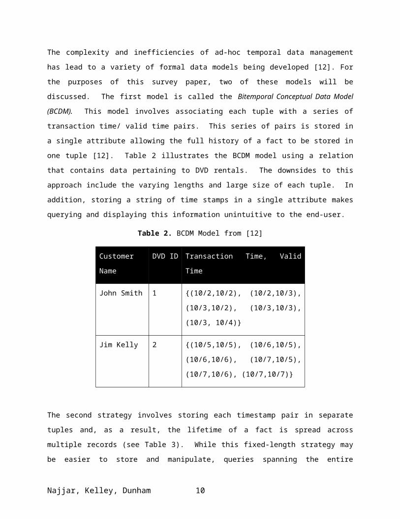
discussed. The first model is called the Bitemporal Conceptual Data Model (BCDM). This model

involves associating each tuple with a series of transaction time/ valid time pairs. This series of pairs is

stored in a single attribute allowing the full history of a fact to be stored in one tuple [12]. Table 2

illustrates the BCDM model using a relation that contains data pertaining to DVD rentals. The downsides

to this approach include the varying lengths and large size of each tuple. In addition, storing a string of

time stamps in a single attribute makes querying and displaying this information unintuitive to the end-

user.

Table 2. BCDM Model from [12]

Customer

Name

DVD ID Transaction Time, Valid Time

John Smith 1 {(10/2,10/2), (10/2,10/3), (10/3,10/2),

(10/3,10/3), (10/3, 10/4)}

Jim Kelly 2 {(10/5,10/5), (10/6,10/5), (10/6,10/6),

(10/7,10/5), (10/7,10/6), (10/7,10/7)}

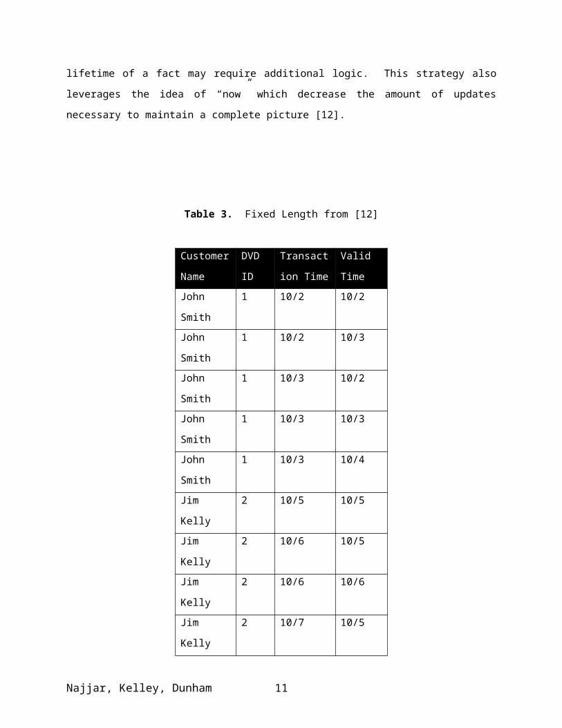
The second strategy involves storing each timestamp pair in separate tuples and, as a result, the lifetime of

a fact is spread across multiple records (see Table 3). While this fixed-length strategy may be easier to

store and manipulate, queries spanning the entire lifetime of a fact may require additional logic. This

strategy also leverages the idea of “now” which decrease the amount of updates necessary to maintain a

complete picture [12].


Table 3. Fixed Length from [12]

Customer

Name

DVD

ID

Transaction

Time

Valid

Time

John Smith 1 10/2 10/2





Jim Kelly 2 10/5 10/5

Jim Kelly 2 10/6 10/5

Jim Kelly 2 10/6 10/6

Jim Kelly 2 10/7 10/5

Jim Kelly 2 10/7 10/6

Jim Kelly 2 10/7 10/7

Many existing query languages (i.e. SQL) can be used to manipulate temporal data but, oftentimes, the

logic required is overly complex. As a result, extensions for existing data manipulation languages (i.e.

TSQL2) and hundreds of temporal languages have been developed to allow for the natural manipulation

of complex temporal ideas [12].

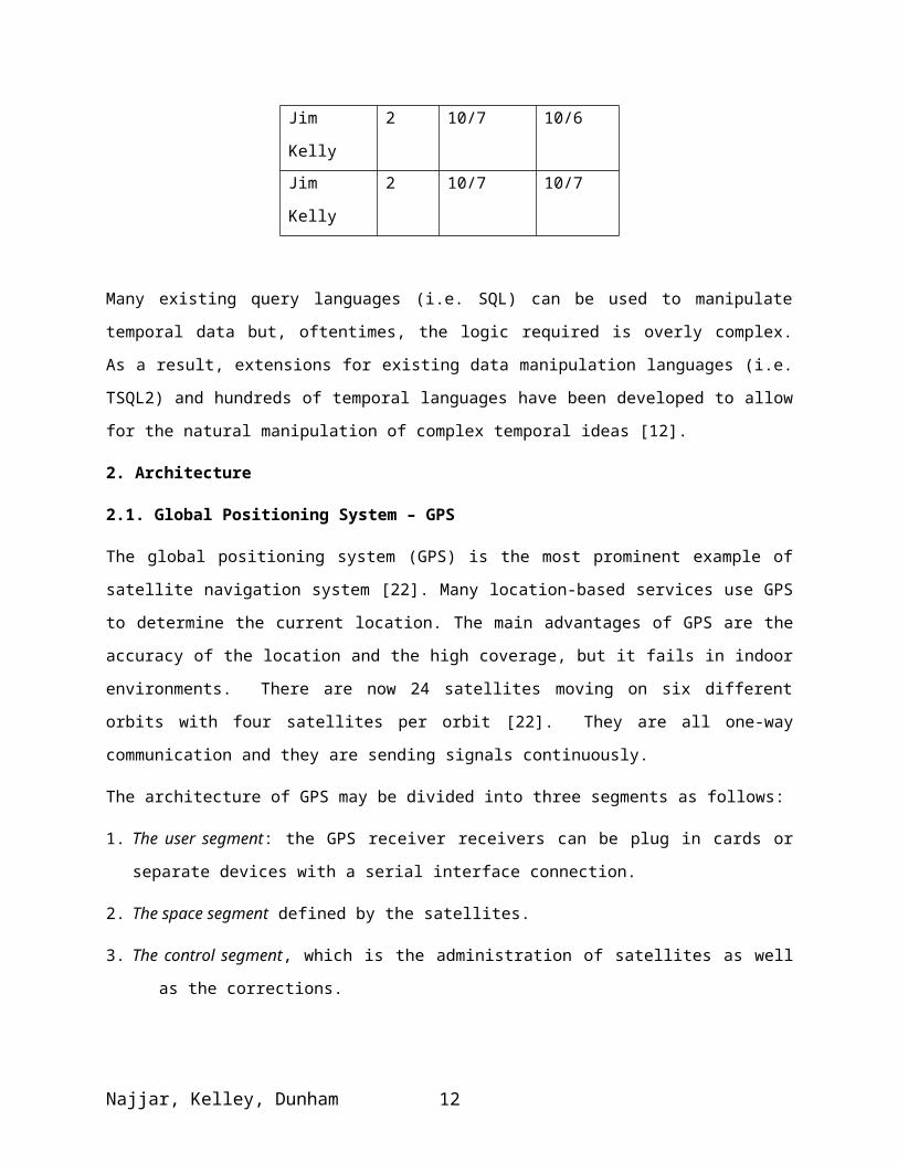
2. Architecture

2.1. Global Positioning System – GPS

The global positioning system (GPS) is the most prominent example of satellite navigation system [22].

Many location-based services use GPS to determine the current location. The main advantages of GPS are

the accuracy of the location and the high coverage, but it fails in indoor environments. There are now 24

satellites moving on six different orbits with four satellites per orbit [22]. They are all one-way

communication and they are sending signals continuously.

The architecture of GPS may be divided into three segments as follows:


1. The user segment: the GPS receiver receivers can be plug in cards or separate devices with a serial

interface connection.

2. The space segment defined by the satellites.

3. The control segment, which is the administration of satellites as well as the corrections.

A mobile user who wants to know his (her) current location, may use GPS signals which are now free of

charge, also the receiver is not expensive. GPS services are classified into two types:

Precise positioning service (PPS), which is not accessible by the civilian users but by the army

forced. It allows a positioning with a precision about 3 meters.

Standard positioning service (SPS) is available for civilian users and it provides, since 2000, the

current location with a precision of 25 meters.

2.2. LDS Middleware Architecture

The middleware architecture discussed in this section comes primarily from [24]. It is typical of work

done in this area.

We use the term Location Dependent Services (LDS) to refer to the software which is responsible for

processing a location dependent data acces. Any LDS design must at least support the following basic

functions:

Bind location to query.

Determine content provider(s) for processing the query.

Translate query location to location used by data.

We assume that the LDS software uses a Location Service (LCS) to determine the location for the query.

As we assume that the LDS is independent of both the content provider and the wireless provider, the

LDS must also determine where to process the query. This could be at multiple content provider

locations. The LDS must then translate the query into a query format understood by each content

provide. We make no assumptions about the type of data and system used by any content provider.

There are three architectural approaches which can be used to support LDS applications:

1. Content Side: Here all LDS support functions are provided by the content provider with the

support of a Location Service (LCS) module. The content provider is responsible for binding the

mobile user's query to a location and then for processing the query itself. Location is assumed to

be the current position of the mobile user. The LCS estimates the mobile user's most accurate

position by using the information stored in the network or the device itself. If the granularity


provided by the LCS is not compatible with the granularity of the stored data, then the content

provider may need to customize its database accordingly. Otherwise, the content provider can ask

for the location of the mobile user at a certain granularity. This approach is simple and suitable

for thin clients with scarce resources, like mobile phones and PDAs. Ericsson's Mobile

Positioning System (MPS) is an example of this type of architecture [5].

2. Wireless Side: Here, support for LDS applications is moved to the wireless operator side.

Wireless operator provides all the functionality to the mobile user in a well defined and limited

way. The mobile user does not know anything about the content provider, all he sees is the menu

provided by his wireless operator.

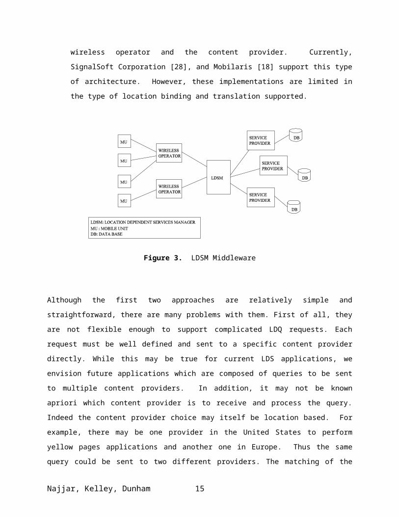
3. Middleware: This approach assumes that a special software agent, Location Dependent Services

Manager (LDSM), sits between the wireless operator and the content (service) provider. This

approach is shown in Figure 3. This software agent performs all LDS functions, with the help of

LCS software, independent of both the wireless operator and the content provider. Currently,

SignalSoft Corporation [28], and Mobilaris [18] support this type of architecture. However, these

implementations are limited in the type of location binding and translation supported.

Figure 3. LDSM Middleware

Although the first two approaches are relatively simple and straightforward, there are many problems

with them. First of all, they are not flexible enough to support complicated LDQ requests. Each request

must be well defined and sent to a specific content provider directly. While this may be true for current

LDS applications, we envision future applications which are composed of queries to be sent to multiple


content providers. In addition, it may not be known apriori which content provider is to receive and

process the query. Indeed the content provider choice may itself be location based. For example, there

may be one provider in the United States to perform yellow pages applications and another one in Europe.

Thus the same query could be sent to two different providers. The matching of the query to a provider

should be dynamic not prewired. Users should be able to use any LDS from any service provider, not

only the ones presented by default from the wireless network.

Besides being independent of the underlying cellular technology, the middleware approach provides a

more flexible and transparent framework for LDS applications. Different location identification software

or LCS can be used in the architecture to locate the mobile user. Unlimited content options can be

provided by this approach which allows access to many different localized information services. We

envision LDS application software providers competing with each other for users. These LDS providers

will use different functionalities and approaches to implement location dependent applications. Users

from different wireless operators may subscribe to the same LDS services.

The middleware design facilitates the implementation of a flexible LDS support service which could

work with multiple wireless operators and content providers. In addition, very complex location binding

can be supported. LDQs of the future will need to have the query bound to locations other than the

current position of the Mobile Unit (MU). There are also some types of queries which need to be

repeatedly requested. For example, suppose a user only wishes to spend the night at a Brand A Hotel. He

could issue a query to be requested periodically to find a Brand A Hotel. This sophisticated type of LDQ

can be supported by a middleware software, but not easily supported by any of the other two approaches.

Other types of queries may be fragmented and sent to different content providers. These subquery results

could then be merged together and returned to the user. The architecture could also use intelligence for

caching results for frequent disconnection cases, or use access patterns for prefetching data and for

efficient use of resources.

3. Overview of Location-Dependent Queries

In this section we provide the definition of location-dependent data/query and then classify the queries.

The term of Location Dependent Data (LDD) can be defined as the data whose value is dependent on

some reference location, which in most cases is the current position of the query’s issuer. A data item

refers to one type of LDD (e.g. restaurants) and usually has different instances. Thus, a data instance is an

answer to the query. Before a mobile user can access information, it is important to consider the location

model, in which location information specified in the user’s query is either explicit or implied in the

query.


The query retrieving LDD is called a Location Dependent Query (LDQ), and the result set of the query

changes depending on the location of the query issuer. The location information is always hidden and

implied by “current location or here”. For example, “find the nearest gas station”.

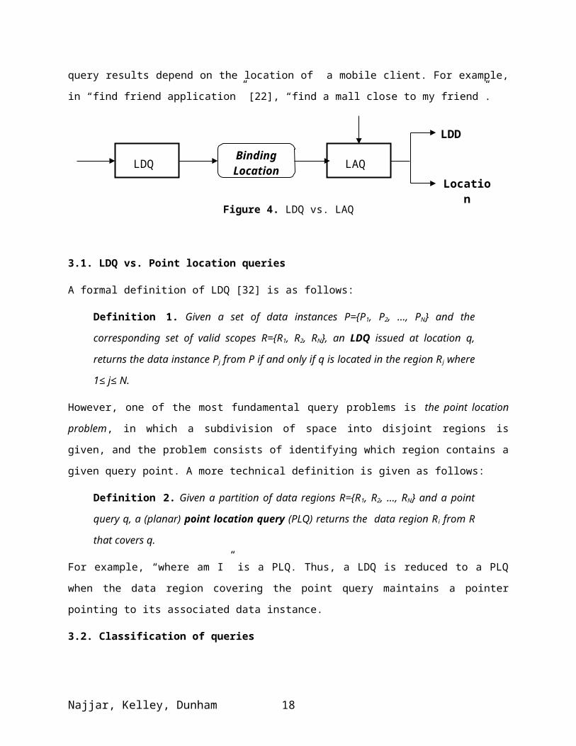
When the user’s location is known (e.g. by GPS), the LDQ can be converted into a Location Aware

Query (LAQ) [23] with an explicit indication of this special location attribute in the query. The process of

obtaining the location information of the query issuer is called Location Binding (see Figure 4). For

examples, “find the nearest hotel of position x Latitude and y Longitude” or “find all Chinese restaurants

in Dallas”. So, LAQ retrieves the same query results independent of the query issuer. Sometimes LAQs

also need location binding if the query results depend on the location of a mobile client. For example, in

“find friend application” [22], “find a mall close to my friend”.

Figure 4. LDQ vs. LAQ

3.1. LDQ vs. Point location queries

A formal definition of LDQ [32] is as follows:

Definition 1. Given a set of data instances P={P1, P2, …, PN} and the corresponding set of

valid scopes R={R1, R2, RN}, an LDQ issued at location q, returns the data instance P j from

P if and only if q is located in the region Rj where 1≤ j≤ N.

However, one of the most fundamental query problems is the point location problem, in which a

subdivision of space into disjoint regions is given, and the problem consists of identifying which region

contains a given query point. A more technical definition is given as follows:

Definition 2. Given a partition of data regions R={R1, R2, …, RN} and a point query q, a

(planar) point location query (PLQ) returns the data region Ri from R that covers q.

For example, “where am I” is a PLQ. Thus, a LDQ is reduced to a PLQ when the data region covering the

point query maintains a pointer pointing to its associated data instance.

3.2. Classification of queries

Najjar, Kelley, Dunham

Location

LDQ LAQ

LDDBindingLocation

12

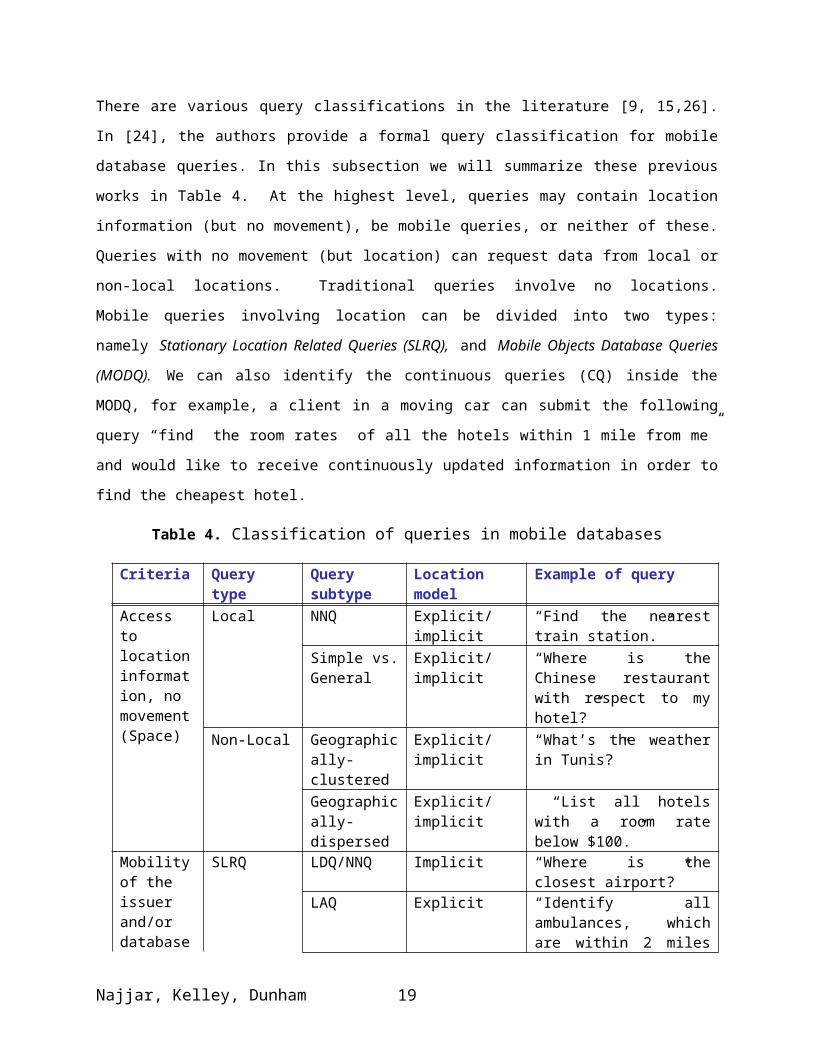
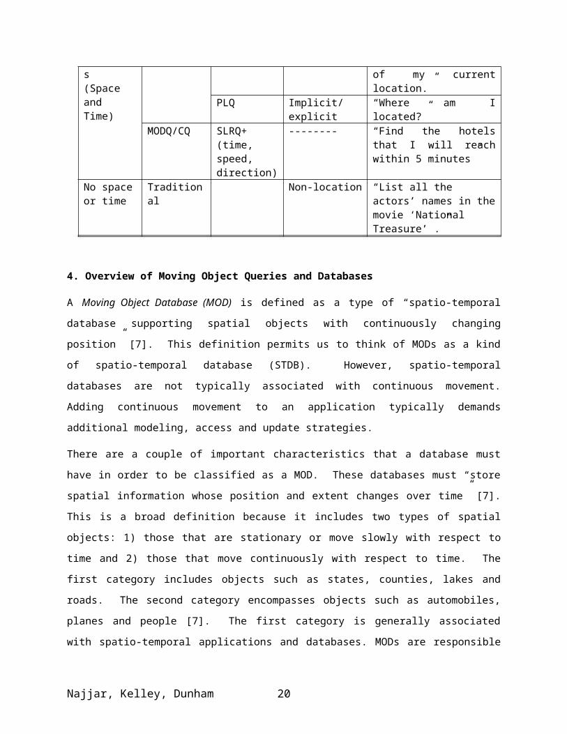
There are various query classifications in the literature [9, 15,26]. In [24], the authors provide a formal

query classification for mobile database queries. In this subsection we will summarize these previous

works in Table 4. At the highest level, queries may contain location information (but no movement), be

mobile queries, or neither of these. Queries with no movement (but location) can request data from local

or non-local locations. Traditional queries involve no locations. Mobile queries involving location can

be divided into two types: namely Stationary Location Related Queries (SLRQ), and Mobile Objects

Database Queries (MODQ). We can also identify the continuous queries (CQ) inside the MODQ, for

example, a client in a moving car can submit the following query “find the room rates of all the hotels

within 1 mile from me” and would like to receive continuously updated information in order to find the

cheapest hotel.

Table 4. Classification of queries in mobile databases

Criteria Query type Query subtype

Location model Example of query

Access to location information, no movement(Space)

Local NNQ Explicit/implicit “Find the nearest train station.”

Simple vs. General

Explicit/implicit “Where is the Chinese restaurant with respect to my hotel?”

Non-Local Geographically-clustered

Explicit/implicit “What’s the weather in Tunis?”

Geographically-dispersed

Explicit/implicit “List all hotels with a room rate below $100.”

Mobility of the issuer and/or databases(Space and Time)

SLRQ

LDQ/NNQ Implicit “Where is the closest airport?”

LAQ Explicit “Identify all ambulances, which are within 2 miles of my current location.”

PLQ Implicit/explicit “Where am I located?”MODQ/CQ SLRQ+(time,

speed, direction)

-------- “Find the hotels that I will reach within 5 minutes”

No space or time

Traditional Non-location “List all the actors’ names in the movie ‘National Treasure’ .”

4. Overview of Moving Object Queries and Databases

A Moving Object Database (MOD) is defined as a type of “spatio-temporal database supporting spatial

objects with continuously changing position” [7]. This definition permits us to think of MODs as a kind

of spatio-temporal database (STDB). However, spatio-temporal databases are not typically associated


with continuous movement. Adding continuous movement to an application typically demands additional

modeling, access and update strategies.

There are a couple of important characteristics that a database must have in order to be classified as a

MOD. These databases must “store spatial information whose position and extent changes over time” [7].

This is a broad definition because it includes two types of spatial objects: 1) those that are stationary or

move slowly with respect to time and 2) those that move continuously with respect to time. The first

category includes objects such as states, counties, lakes and roads. The second category encompasses

objects such as automobiles, planes and people [7]. The first category is generally associated with spatio-

temporal applications and databases. MODs are responsible for storing and manipulating both types of

objects described above and it is the second class of objects that makes this technology so unique.

MODs store the position of objects in space. Some of those objects move through space while others are

stationary. For example, an application used to manage a fleet of delivery trucks would focus on tracking

the delivery trucks (moving objects) as they travel through the streets (stationary objects) of a particular

city (stationary objects). As time moves forward, an object may change its position within space

affecting the spatial relationship between that object and the other objects found within the database. [6].

A moving object has a starting position, which is a point in space denoting the beginning of a route. That

starting position can be coupled with a start time. In addition, a line through space is used to represent an

object’s route. The end position of a route may or may not be known beforehand. Other characteristics

such as trajectory, velocity and acceleration may also be associated with a moving object [27].

There are many operators that are commonly used to manipulate and understand moving objects. The

operator IN can be used to determine whether or not and object is within a region at a given point in time.

It may also be necessary to determine if an object is entering or exiting a region. Furthermore, it might be

important to identify whether two objects are moving away or towards one another. Similarly, two

objects moving towards each other may collide. Catching up may be used to describe two objects that are

moving in the same direction with the distance between those objects decreasing. Opposite direction

would imply that two objects are moving away from each other. Meet considers two objects with the

same speed and requires that the faster object has a negative acceleration, the slower object has a positive

acceleration or both [25].

Because the entities being tracked in MODs are continuously changing in regards to space and time, the

location of an object is intrinsically uncertain and this idea is generally referred to as “location

uncertainty”. Moreover, regardless of how frequently a moving object’s current position is updated

within the database, the database location will never be the same as the actual location. As a result, it

may be necessary to qualify and/or quantify that uncertainly using “must” or “may” semantics.


Specifically, it might be necessary to differentiate between all objects that must satisfy a query predicate

and all objects that may satisfy a query predicate. Furthermore, a probability could be used identify the

likelihood that a result may satisfy a query [28].

Queries against MODs can fall into a number of categories. First, range queries can be described as

requesting objects that fall within a given spatio-temporal range. For example, one might request all

vehicles within 5 miles (spatial predicate) of a bank robbery between 2-3p.m. (temporal predicate) [18].

Next, nearest neighbor (kNN) queries are interested in objects that are within a defined proximity to some

point in space. The nearest neighbor predicate is typically applied to the spatial dimension or the

temporal dimension but not to both. The kNN predicate is then coupled with a range predicate to be

applied to the other dimension. To clarify, a temporal kNN query might be something like “retrieve the

first 10 vehicles that were within 100 yards (spatial range) from the scene of the accident ordered based

on the difference between the time the accident occurred and the time the vehicle crossed the spatial

region (temporal kNN predicate)” [18]. Generally, temporal kNN queries are interested in the most

recent past or some point in the future but rarely in both, allowing the query to concentrate on one portion

of the time dimension. A spatial kNN query might ask to “retrieve the five ambulances that were nearest

to the location of the accident (spatial kNN predicate) between 4-5 p.m. (temporal range) [18]. Join

queries are traditionally used to detect or predict the collision or the overlap of either two moving objects

or a moving object and a stationary object. For example, join queries can be used by flight controllers to

estimate the effects of a flight pattern reconfiguration during an emergency in an effort to avoid any in-

flight collisions.

There are a couple of additional nuances that are typically associated with querying MODs that are worth

mentioning. First, one may to choose to limit the perspective of a query in regards to the time dimension.

It may be necessary to only focus on the historical positions of an object. In contrast, it is also common to

focus on the current and future positions of an object, which requires associating that object with a

function of time. That function could take velocity and trajectory into consideration when estimating the

future position of an object. It may also be feasible to obtain a “reservation” from each object that

specifies the spatial destination. This greatly reduces the complexity of predicting the future positions of

objects. Splitting queries along these lines is oftentimes necessary because the techniques in regards to

indexing and optimization can be different. In addition, because the locations of moving objects are

continuously changing, these locations are inherently uncertain [28]. For example, one may wish to

“retrieve the friendly helicopters that are expected (according to the current speed and direction

information) to enter a stated region in the next hour. “ It might be necessary to apply “must” or “maybe”

semantics to this query. The latter would be coupled with some “uncertainty bound” or probability that


dictates the acceptable threshold for incorrect predictions. For example, the reply to a query using an

uncertainty bound is “m is on route 968 at location (x, y) with an error or deviation of at most 2 miles”.

Furthermore, the database engine might commit to send a location update when some deviation is reached

[28].

First, moving object databases and applications are being used extensively in the field of mobile

workforce management. Location tracking is combined with predetermined route information to manage

mobile devices such as planes, trains, delivery trucks and taxis. Call centers can use these applications to

optimize resource utilization, determine delivery times and react to extenuating circumstances such as bad

weather or traffic congestion [27]. For example, a database used to track the location of taxis might need

to know all free cabs within a one-mile radius of a given customer. Likewise, a delivery service might

need to alter a route(s) for a special delivery and would do this by first determining all routes that fall

within a certain distance of that address.

Another application for moving object databases is called Location-Aware Content Delivery. The origins

of this technology lie in a field called “Context Aware Computing”. These applications use a mobile

device such as a cell phone to provide location information. That information can then be combined with

contextual information such as the time of day, current weather conditions, nearby locations and the

mobile users’ current activities [2]. Ultimately, content is tailored based on that contextual information

and sent to that mobile device. This content might include coupons for local stores, information on

surrounding tourist attractions and restaurant reviews [2].

Finally, moving object technology is oftentimes used in the digital battlefield. Military leaders have

realized that the key to winning a war is to create a fast and accurate information delivery system [19].

The aim of battlefield analysis is to collect and analyze information about things such as enemy location

and movement, characteristics of the terrain and weather conditions [19]. These applications leverage

distributed computing solutions that seek to track mobile objects in an environment where network

bandwidth is scarce [3]. Data may come from a wide variety of sources including satellites,

reconnaissance drones and mobile devices worn by ground troops. The application should integrate that

data into a unified view and allow key decision makers to adjust their strategies accordingly. For

example, it may be necessary to determine all friendly aircraft that can be expected to enter a region in the

near future [27]. In the event of an emergency, this would allow decision makers to determine if it is best

to pull out due to a lack of adequate air support or stay in place because assistance will arrive in a timely

manner.


5. Location Modeling and Translation

As indicated earlier, any LDQ must involve either an explicit or implicit location. However, there are

many ways to view a location: latitude/longitude, street address, zip code, etc. An even bigger problem

is that different systems entities involved in processing the LDQ may have different views. Different

content providers could store data at different location granularities. The LCS could bind the location to

yet a third. This difference between location granularities is referred to as the Location Granularity

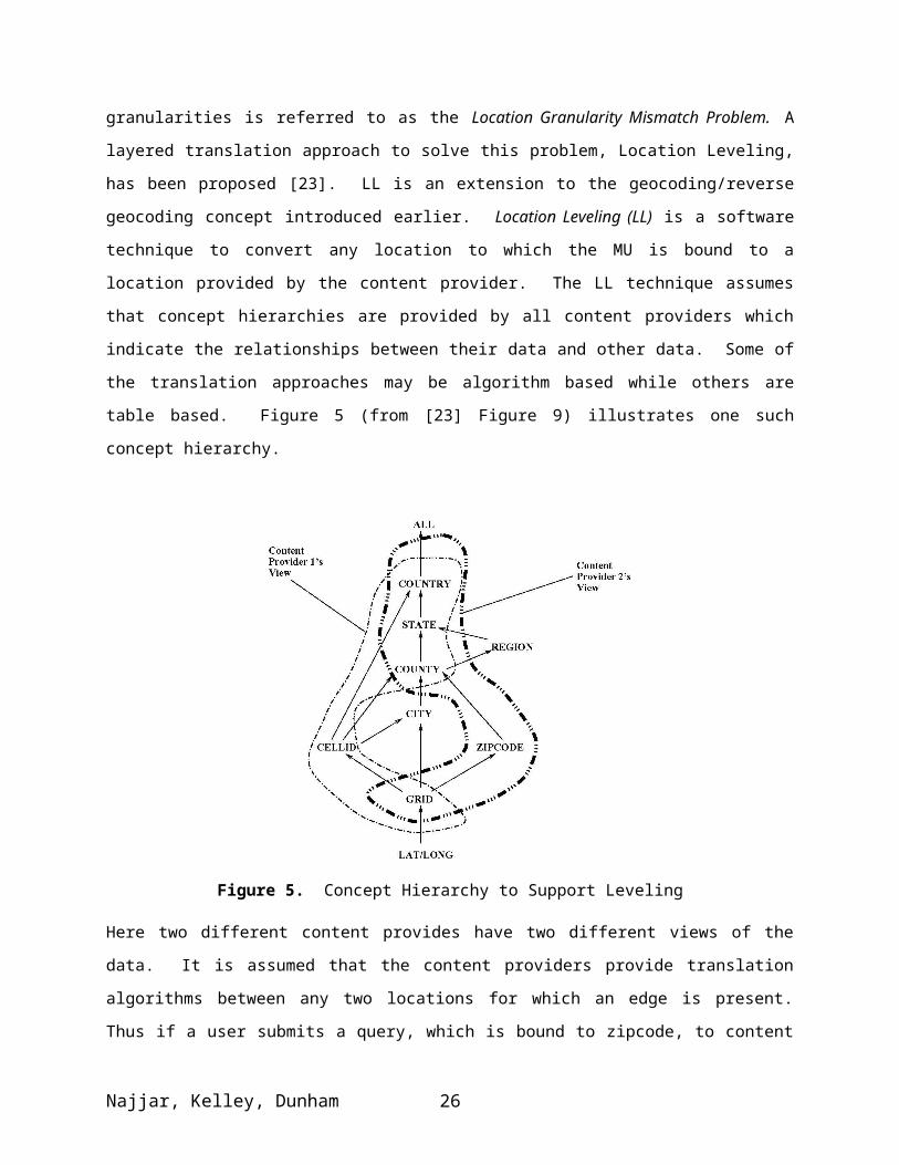
Mismatch Problem. A layered translation approach to solve this problem, Location Leveling, has been

proposed [23]. LL is an extension to the geocoding/reverse geocoding concept introduced earlier.

Location Leveling (LL) is a software technique to convert any location to which the MU is bound to a

location provided by the content provider. The LL technique assumes that concept hierarchies are

provided by all content providers which indicate the relationships between their data and other data.

Some of the translation approaches may be algorithm based while others are table based. Figure 5 (from

[23] Figure 9) illustrates one such concept hierarchy.

Figure 5. Concept Hierarchy to Support Leveling

Here two different content provides have two different views of the data. It is assumed that the content

providers provide translation algorithms between any two locations for which an edge is present. Thus if

a user submits a query, which is bound to zipcode, to content provider 2 where the data in the

corresponding database is at the county granularity, a translation from zipcode to county would be

required to determine which counties satisfy the proposed query.


6. Nearest-neighbor Queries Through Point Location and Indexing

Nearest-neighbor (NN) searching is an important problem in a variety of applications, including

multimedia databases, document retrieval, knowledge and data mining, pattern recognition and

classification, machine learning and statistics. The NN search (e.g. finding the nearest gas station) can be

seen as LDQ problem when the solution space is precomputed (e.g. by Voronoi diagram). So, in order to

determine the closest site, it suffices to first compute the subdivision induced by the Voronoi diagram and

then generates a point location data structure for Voronoi diagram. In this way, the nearest-neighbor

queries (NNQ) are reduced to PLQ.

We start this section by giving some preliminaries about Voronoi diagrams and then exploring the use of

indexes to facilitate efficient evaluation of LDQ in mobile and wireless environment.

6.1.Voronoi diagram

The concept of Voronoi diagram is used extensively in a variety of applications, including robotics,

knowledge discovery and data mining, classification, multimedia databases, document retrieval and

statistics and many other fields.

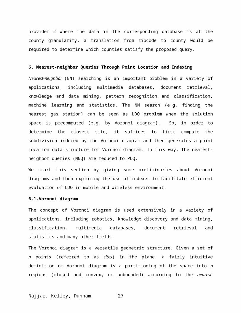
The Voronoi diagram is a versatile geometric structure. Given a set of n points (referred to as sites) in the

plane, a fairly intuitive definition of Voronoi diagram is a partitioning of the space into n regions (closed

and convex, or unbounded) according to the nearest-neighbor rule: each site gets assigned the region

which is closest to (see Figure 6).

Figure 6. The Voronoi diagram of a set of points.


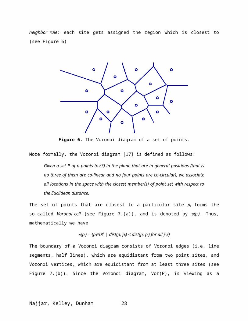
More formally, the Voronoi diagram [17] is defined as follows:

Given a set P of n points (n≥3) in the plane that are in general positions (that is no three

of them are co-linear and no four points are co-circular), we associate all locations in

the space with the closest member(s) of point set with respect to the Euclidean distance.

The set of points that are closest to a particular site pi forms the so-called Voronoi cell (see Figure 7.(a)),

and is denoted by (pi). Thus, mathematically we have

(pi) = {pIR2 | dist(p, pi) < dist(p, pj) for all j≠i}

The boundary of a Voronoi diagram consists of Voronoi edges (i.e. line segments, half lines), which are

equidistant from two point sites, and Voronoi vertices, which are equidistant from at least three sites (see

Figure 7.(b)). Since the Voronoi diagram, Vor(P), is viewing as a planar graph, every vertex in a Vor(P)

has degree 3 (i.e. exactly three Voronoi edges are incident to it).

Figure 7. (a) A Voronoi cell of pi (filled region). (b) A Voronoi diagram in a bounded box.

The union of the boundaries of the Voronoi cells is the Voronoi diagram which we refer to as Vor(P).

Note that adjacent Voronoi cells overlap only on their boundaries.

Now that we understand the structure of the Voronoi diagram we present its complexity in terms of the

total number of vertices and edges.

Property [1, 17]: for n≥3, the number of vertices in the Voronoi diagram of a set of n

point sites is at most 2n-5 and the number of Voronoi edges is at most 3n-6.

So, Voronoi diagram has a linear complexity.


pi

P4

P1

P2

P3

P5

P6 P

8

P7

(b) (a)

The Voronoi diagram serves as the basis for nearest-neighbor queries: each query is a point in the space

containing N sites and we are required to report the closest site to the query point. In such cases, it

suffices to compute first the Voronoi diagram and then to generate a point location data structure for the

Voronoi diagram. Consequently, the problem of LDQ can be reduced to the problem of PLQ.

6.2. Related work in indexing techniques

We explore the use of index on simple shapes, which in general perform efficiently in mobile and

wireless environment. The indexing problem of LDQ consists of: given the valid scopes (Voronoi cells)

of all data instances of a certain query type, how we can index them to allow efficient processing of LDQ

through PLQ.

The goal of PLQ is to preprocess a subdivision into a data structure which provides an optimal O(n) space

and O(logn) query time for answering PLQ in the plane. Several indexing techniques for PLQ exist in

the literature. There are typically two well known types of index techniques, namely object

decomposition and object approximation. The former is based on the pre-computed solution space, it is

also called solution-based index. Especially, for NN search, the solution space can be represented by valid

scopes (e.g. Voronoi diagrams). Whereas the latter represents a simple approximation of each data region,

it is also called object-based index, because it is built on object locations. The most commonly index used

in GIS is the Minimal Bounding Box (MBB) or Minimal Bounding Rectangle (MBR).

In the following subsections we briefly review the existing indexing approaches and then introduce our

new index structure for LDQ. Most of the decomposition techniques are based on the principle of

recursive hierarchical partition. We assume for the following subsections that a polygonal subdivision

(that is, a Voronoi diagram) contains n vertices and m edges.

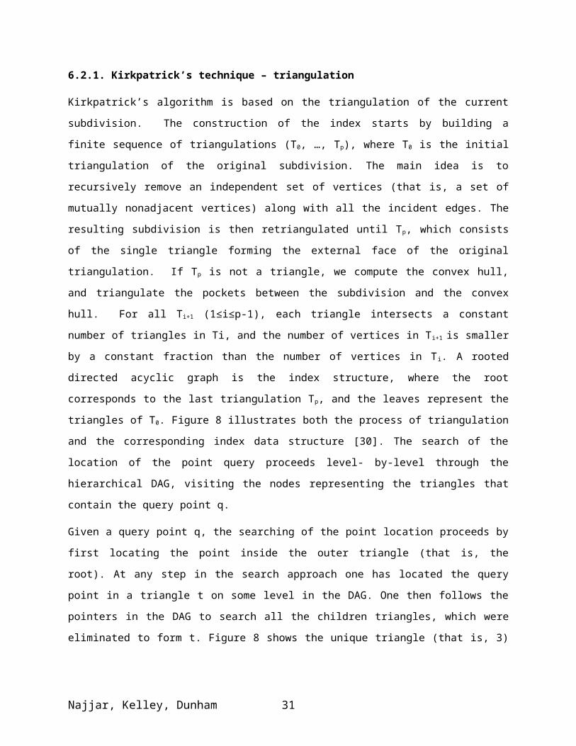
6.2.1. Kirkpatrick’s technique – triangulation

Kirkpatrick’s algorithm is based on the triangulation of the current subdivision. The construction of the

index starts by building a finite sequence of triangulations (T0, …, Tp), where T0 is the initial triangulation

of the original subdivision. The main idea is to recursively remove an independent set of vertices (that is,

a set of mutually nonadjacent vertices) along with all the incident edges. The resulting subdivision is then

retriangulated until Tp, which consists of the single triangle forming the external face of the original

triangulation. If Tp is not a triangle, we compute the convex hull, and triangulate the pockets between the

subdivision and the convex hull. For all Ti+1 (1≤i≤p-1), each triangle intersects a constant number of

triangles in Ti, and the number of vertices in T i+1 is smaller by a constant fraction than the number of

vertices in Ti. A rooted directed acyclic graph is the index structure, where the root corresponds to the last

triangulation Tp, and the leaves represent the triangles of T0. Figure 8 illustrates both the process of


triangulation and the corresponding index data structure [30]. The search of the location of the point

query proceeds level- by-level through the hierarchical DAG, visiting the nodes representing the triangles

that contain the query point q.

Given a query point q, the searching of the point location proceeds by first locating the point inside the

outer triangle (that is, the root). At any step in the search approach one has located the query point in a

triangle t on some level in the DAG. One then follows the pointers in the DAG to search all the children

triangles, which were eliminated to form t. Figure 8 shows the unique triangle (that is, 3) containing q.

The visiting nodes are in the path of 20, 18, and finally the triangle 3.

Figure 8. The sequence of triangulation generated by Kirkpatrick’s approach and its

corresponding DAG for searching.

6.2.2. Trapezoidal map

Trapezoidal Map or decomposition (and sometimes known as the vertical decomposition) of the space S,

which is viewed as a collection of line segments. The trapezoidal map is obtained by passing a vertical

line through each end-point pi of each segment in S, going upwards and downwards until it hits another

segment of S. Some of these lines will continue to infinity, because they do not hit any other line

segments. We assume henceforth that:


1. the entire domain is enclosed in a large bounding box, in order to avoid infinite lines, and

2. the x-coordinates of the segments are all distinct, in order to avoid degeneracy.

Thus, the process of randomized incremental construction of the trapezoidal map is described by the

following steps:

Input: a set S of m planar line segments, that is, S=(s1, s2, …, sm) – a random order.

Output: the trapezoidal map T(S) and a search data structure D (rooted DAG).

1. for i from 1 to m do

2. find the set 0, … k, of trapezoid in T properly intersected by si

3. remove from T and replace them by new trapezoids that appeared after the insertion of si.

4. Remove the leaves from D, and create new leaves from the current found trapezoids – that is, to

link internal nodes to new leaves with respect to the history of the randomized construction

(explained below).

We now describe the point location data structure, which is based on a rooted directed acyclic graph.

Each internal node consists of two types of nodes: the x-nodes or the y-nodes. Each x-node, represented

by circles, contains the x-coordinate x0 of an endpoint of one of the segments, and its two children

correspond to the neighbor points lying to the left and right of x-coordinate (that is, x=x0). Each y-node,

represented by hexagon, contains a pointer to a line segment of the subdivision. The left and right

children of a y-node correspond to the space above and below the line segment represented by the y-node

(see Figure 9). The leaves represent the trapezoids.

Figure 9. Construction of trapezoidal map and its associated DAG


Given a query point q, the search process begins at the root and terminates when a leaf node is reached.

At x-node, we evaluate whether q lies to the left or to the right of the vertical line defined by the stored x-

coordinate. At a y-node, we evaluate whether q lies above or below the segment. This is illustrated in

Figure 9. For further details see [1, 15].

6.2.3. K-d trees

The k-d tree is one of the most prominent d-dimensional data structures [8, 15]. Perhaps the most popular

class of indexing technique to the NN search structure involves some sort of hierarchical space

decomposition. It is a binary search tree that represents a recursive subdivision of the universe into

subspaces by means of (d-1)-dimensional hyperplanes. The hyperplanes are iso-oriented, and their

direction alternates between the d possibilities. For d = 3, for example, splitting hyperplanes are

alternately perpendicular to the x-, then y-, then z-axis and then back to x-, and so on. The choice of the

splitting rule is an important issue in the implementation of the k-d tree. A good split is one that divides

the points into subsets of roughly equal sizes, and which produces cells containing at least one data point.

Internal nodes contain the axis-orthogonal splitting hyperplane and have one or two children representing

the rectangular subcells (see Figure10). The leaves store all the data points. Searching and insertion of

new points are straightforward operations. Deletion is somewhat more complicated and may cause a

reorganization of the sub-tree below the data point to be deleted. Note that it is difficult to keep the tree

balanced in the presence of frequent insertions and deletions. The structure works best if all the data is

known a priori and if updates are not frequent.

Figure 10. An example of a k-d tree (right) and its corresponding spatial subdivision (left).

One disadvantage to a k-d-tree is that for certain distributions no hyper-plane can be found which splits

the data points evenly.

The construction of a k-d tree is briefly described as follows: we first compute the median of the point set

in one of the dimensions, say x-axis and partition the point set into two subsets based on the median point


q

p4 p5 p9p10

p2

p1

p3p6

p7

p8

23

p10 p9p8

p7p6

p5 p4

p2p1

p3

(that is, all the points having coordinates less than the median point along x-axis are placed in one subset

– left and the remaining points are placed in the other subset – right). This process is then recursively

continued along the other y-axis in the resulting cells. Once the partitioning is completed along all the

axis, it is repeated back to x-axis and so on until there is only one data point.

The general advantage of k-d tree is that the decision of which sub-tree to use is always unambiguous.

The search in kd-tree is not the most efficient, the search algorithm visits all the nodes containing the

query point q and maintains the closest point to q. Since the root represents all the space region, it has to

go first to a leaf (say pi), which is the initial closest point to q. And then it would visit the parent and all

the nodes intersecting the circle centered at q of radius distance(q, p i). If the distance is greater than the

distance of the closest point encountered so far, the search returns immediately. In Figure 10, with a query

point q, the search algorithm first finds the closest point p3 (with a deep search). The visited points in kd-

tree are in italic. The final answer is p2.

6.2.4. D-tree

The D-tree is reported [30] to have a better performance for indexing solution-space than traditional

indexes. The D-tree is a binary height-balanced tree. It is similar to the kd-tree. However, while the kd-

tree is built based on hyperplanes, the D-tree is constructed based on the division that form the boundaries

of the valid scopes. For a space containing a set of valid scopes that are disjoint and complementary, it

recursively partitions the space having similar number of scopes until a space has one scope only. The

partition between two subspaces is represented by one or more polylines. Figure 11 (a) shows a valid

scope for 4 objects. Polyline pl(v2, v3, v4, v6) partitions the original space into P5 and P6 and pl(v1, v3) and

pl(v4, v5) further partition P5 into P1 and P2, and P6 into P3 and P4, respectively.

Figure 11. Index construction using the D-tree. (a) Divisions in the index. (b) D-tree structure [30]


v1

v4 v5

P3

v6

P1

P4P2

v5

v4

v3

v2

P6P5

1 Y

P6

v2 v3 v4 v8

2 X v1 v3 2 X

P5

P1 P2 P3 P4

To data instances

(a) (b)

24

LSF RSFLeft_ptr Right_ptr

Dim : Partition dimensionLSF : Left sites frontierRSF: Right sites frontier Left_ptr: pointer to the left childRight_ptr: pointer to the right child

Dim

Figure 11 (b) shows the corresponding D-tree. Each node of the D-tree contains a header attribute, the

partition that divides the space into two complementary subspaces and two pointers (left and right). The

searching on the D-tree starts from the root, and recursively follows either the left pointer or the right

pointer according to the partition and the position of the query point, until a leaf is reached, containing a

pointer to the data instance corresponding to the region.

6.3. The N-tree: a new index structure for LDQ

One of the original motivations for the Voronoi diagram is nearest-neighbor searching. We propose a new

index structure, called N-tree (Neighbors tree), which indexes data regions based on the neighboring in

the solution space represented by Voronoi diagram. But N-tree can also be applied to any planar

subdivision or valid scopes. N-tree is a balanced binary space partitioning tree (BSP), similar to D-tree

[29, 30]. However, while the partition in D-tree is based on polylines, the N-tree is based on the frontier

represented by a set of neighbors which cover the other sites. Since each point in 2-dimension space has

two values (x and y-coordinate), we have to sort and split on x-coordinate or y-coordinate according to

the minimum cardinality of the frontier. We recursively partition a space consisting of a sorted set of data

instances (sites) into two complementary subspaces (left subspace and right subspace) containing about

the same number of sites until each subspace has one site only. The data structure of N-tree is given by

the Figure 12.

Figure 12. Data structure of the N-tree node

N-tree index is based on both object and space solution, that is, instead of storing the boundaries

of valid scopes, it stores the object locations of adjacent sites. Our index structure can be considered as a

hybrid index, because it combines both object and solution based indexes. We are inspired by the

Delaunay triangulation [1, 17], the straight line dual of Voronoi diagram, where the objects are

represented by vertices and 2 objects are connected (edge) if and only if their valid scopes are adjacent.


Thus, we define the frontier set of neighbors to be the set of edges <p i, pj>, one end-point in each of the

frontier sites LSF and RSF. And than, we have to verify that LSF (resp. RSF) cover all the sites in the left

subspace (resp. right subspace), that is LSF and RSF are sufficient to guide a query point to the

appropriate subspace (LS—left sites or RS—right sites). .

Before describing the partition algorithm, we first illustrate it by an example (see Figure 13.).

Figure 13. Construction of N-tree on the example given on Figure 7.

The idea of the construction of the hierarchical partition and its associated index N-tree is as follows:

Input :

S, a set of sites (sorted on increasing order of x-coordinates (Sx) and simultaneously Sy sorted on

decreasing order of y-coordinates), the cardinality of S is N.

E, a set of neighbors <pi, pj> (sorted respectively on x-coordinates, Ex, and y-coordinates, Ey),

the cardinality of E is m – the number of edges in the Voronoi diagram generated by N

points).

Output : N-tree

1. For each partition dimension (x/y)

2. partition S into 2 complementary subsets LS and RS.

3. Find the frontier F – Retrieving from E the edges with one end-point in each of the two sets

LS and RS.

4. Choose the partition with the minimal cardinality of the F.

5. Find LSF –the left sites frontier (resp. RSF –the right sites frontier)

6. Update LE and RE, the edges respectively of the left subset and the right subset.

7. Verify that LSF (resp. RSF) covers the remaining sites of LS (resp. RF)

8. Partition on LS and LE – recursive partition on the left subset


P2 P3 P4 P5 P6 P7 P8

P3P4 Y P8 P7

X

P1P2 X

P1 P2 P3 P4 P6 P8 P7 P5

P4

P1

P2

P3

P5

P6

P8

P7

9. Partition on RS and RE –recursive partition on the right subset

The search algorithm starts from the root, it computes the Euclidean distance from the query point q to the

associate points of this node then recursively follows either the left pointer or the right pointer according

to the minimal distance found (in LSF or RSF). If the number of sites in an internal node is equal to the

sum of all points in this node, the search returns immediately the closest point instead of reaching the leaf.

In the example of Figure 13, for any point query point, the search stops at level 1 (for the best case) and

level 2 (for the worst case) of the tree because the number of sites in the sub-tree at level 1 is equal to 4

and that the number of points in that node is equal to 4. So, in general, the worst case to get the closest

site is (log(N)-1).

6.4. Summary of indexing techniques

Indexing techniques are briefly summarized in Table 5, where N is the number of regions (data instances

or sites), n is the number of vertices and m is the number of segments in the polygonal subdivision.

Table 5. Summary of different indexing techniques for LDQ

Kirkpatrick Trapezoidal kD-tree D-tree N-treeIndex data structure Rooted DAG Rooted

DAG Binary tree Balanced BSP tree Balanced BSP tree

Construction approach – Recursive partitioning

Triangulation Randomized incremental

Hierarchical space decomposition



Construction complexity O(nlogn) O(mlogm) O(NlogN) O(N2logN +N2 +

mN)O(N2logN + Nmlogm + Nm)

Search time complexity (number of nodes visited)

O(logn) O(logm)>O(logN)≤O(N+k) [1]

O(logN) O(logN)

RemarksEasy to understand; Not practical

Simple; Practical

General purposes; Not efficient

Good performance

Efficient storage and retrieval

Applications-- Point location problems

Binary search NN search NN search

Geometric retrieval problems

NN search NN search

7. Conclusions

In this paper we have provided a brief overview of location dependent data access, including LDQs,

MODs, NN queries, and point queries. We have also examined indexing techniques to be used for them.

A major emphasis of this paper was on nearest-neighbor queries.


References

[1] M. Berg, M. V. Kreveld, M Overmars, O. Schwarzkopf. Computational Geometry: Algorithms and Applications. Springer-Verlag, Berlin Germany, 2nd Edition, 2000.

[2] G. Chen, D. Kotz, David "A Survey of Context-Aware Mobile Computing Research." Dartmouth Computer Science Technical Report TR2000-381. 16 September 2002.

[3] X. Chamberlain, “Model-based battle command: A paradigm whose time has come,” Proceedings of the 1st Intenrational Sympostum on Command and control Research and Technoglogy, pp 31-38, 1995.

[4] M. H. Dunham, V. Kumar, “Location Dependent Data and its Management in Mobile Databases,” Proceedings of the Ninth International Workshop on Database and Expert Systems Applications, August 1998, pp 414-419.

[5] Ericsson,”Ericsson Mobile Positioning System”, 2000, http://www.ericsson.se/wireless/products.

[6] M. Erwig, M. Schneider. “Developments in Spatio-Temporal Query Languages.” DEXA Workshop Proceedings, pages 441-449, 1999.

[7] L. Forlizzi, R.H. Guting, E. Nardelli, and M. “A Data Model and Data Structures for Moving Objects Databases.” Technical Report Informatik 260, FernUniversitat Hagen, 1999.

[8] V. Gaede and O. Gunther. Multidimensional Access Methods. ACM Computing Surveys, Vol. 30(2), June 1998.

[9] M. Gupta, N. Tang and A. Pasos. “Query Processing Issues in Mobile Databases”, Term paper in Distributed Database Systems- ESS265 Spring 2003. http://sirius.cs.ucdavis.edu/teaching/

[10] R. H. Guting. “An Introduction to Spatial Database Systems.” The VLDB Journal. 3.4 (October 1994): 357-399. New Jersey: Springer-Verlag.

[11] The Board of Trustees of the University of Illinois, “General Relativity”. Science for the Millennium Expo. 1995. NCSA. http://archive.ncsa.uiuc.edu/Cyberia/NumRel/GenRelativity.html

[12] C. S. Jensen, Christian. “An Introduction to Temporal Database Research.” Ph.D. Dissertation, Arizona U. 2000.

[13] M. Koubarakis, T. Sellis et al. eds. Spatio-Temporal Databases: The Chorochronos Approach. New York: Springer, 2003.

[14] U. Kubach, C. Becker, I. Stepanoo and J. Tian. “Simulation Models and tools for Mobile Location-Dependent Information Access”. Chapter 12, in


http://archive.ncsa.uiuc.edu/Cyberia/NumRel/GenRelativity.html

Mobile Computing Handbook, Mohammad Ilyas and Imad Mahgoub, Editors, Auerbach Publications, 2005.

[15] D. Lee, W.-C. Lee, J. Xu and B. Zheng. “Data Management in Location-Dependent Information Services: Challenges and Issues”. IEEE Pervasive Computing, vol. 1, no. 3, pp. 65-72, July-Sept. 2002.

[16] D. P. Mehta, S. Sahni. Handbook of Data Structures and Applications. Chapman & Hall/CRC 2005.

[17] J. S. Narr. G. LaRocque, “Approaching the Digital Battlefield”. Washington D.C. December 1996.

[18] Mobilaris, “Mobilaris AB – Location Services,” 2000,http://www.mobilaris.se.

[19] A. Okabe, B. Boots, K. Sugihara, and S. N. Chiu. Spatial Tessellations: Concepts and Applications of Voronoi Diagrams. John Wiley & sons, UK, 2nd Edition 2000.

[20] K. Porkaew, Kriengkrai, I.Lazaridis and S.Mehrotra. “Querying Mobile Objects,” in Spatio-Temporal Databases. Berlin: Springer-Verlag, 2003.

[21] K. H. Ryu, Y. Ae Ahn. “Application of Moving Objects and Spatiotemporal Reasoning.” A Time Center Technical Report, TR-58. May 29, 2001.

[22] J. Schiller and A. Voisard. Location-Based Services. Morgan Kaufmann, 2004.

[23] A. Y. Seydim, M. H. Dunham, and V. Kumar, “Location Dependent Query Processing,” May 2001, Proceedings of Mobide, pp 47-54.

[24] A. Y. Seydim, M. H. Dunham, and V. Kumar, “An Architecture for Location Dependent Query Processing,” September 2001, Proceedings of DEXA, pp 549-555.

[25] A. Y. Seydim and M. H. Dunham, “Location Leveling”, submitted to IEEE Transactions on Knowledge and Data Engineering, January 2004, under second round of reviews.

[26] A. Y. Seydim and M. H. Dunham. “Location-Dependent Query Processing in Mobile Computing,” Chapter 11 in Mobile Computing Handbook, Mohammad Ilyas and Imad Mahgoub, Editors, Auerbach Publications, 2005, pp 255-274..

[27] J. Su, H. Xu, and O. Ibarra. Moving objects: Logical relationships and queries. Proc. Int. Sym. on Spatial and Temporal Databases, pages 3-19, 2001.

[28] Signalsoft, SignalSoft Corporation - Wireless Location Services,” 2000,http://www.signalsoftcorp.com.


http://www.signalsoftcorp.com/

http://www.mobilaris.se/

[29] O. Wolfson, S. Chamberlain, S. Dao and L. Jiang. “Location Management in Moving Object Databases.” Proceedings of WOSBIS, October 1997.

[30] O. Wolfson, Ouri, S. Chamberlain, B. Xu and L. Jiang. “Moving Object Databases: Issues and Solutions.” Proceedings of the 10th International Conference on Scientific and Statistical Database Management, April 1998.

[31] J. Xu, B. Zheng, W-C. Lee and D. L. Lee. Energy Efficient Index for Querying Location-Dependent Data in Mobile Broadcast Environments. Proc. Of the 19th Int. Conf. on Data Eng. (ICDE’03), Mar. 2003, pp. 239-250.

[32] J. Xu, B. Zheng, W-C. Lee and D. L. Lee. The D-tree: an index structure for planar point queries in location-based wireless services. IEEE TKDE, vol. 16, No 12, Dec. 2004.

Dr. Faïza NAJJAR received her PhD in Computer Science from the University of Tunis ElManar, Tunisia, in June 1999. Her Ph.D. was prepared with a partnership between France (ENS-Lyon) and the Faculty of Sciences of Tunis. Since 2000, she has been an Assistant Professor at the National School of Computer Science and Engineering in Manouba (Tunisia). Her current areas of research include mobile computing and databases, computational geometry (especially Voronoi diagrams and triangulation), and distributed query processing on the grid.

Sean Kelley received his M.S. degree in Computer Science from Southern Methodist University in May 2005. His concentration was in databases and data mining. He received a B.S. Business Administration-MIS degree from the University of Texas at Austin in 2002. He has extensive experience as a data warehouse architect and consultant.

Margaret (Maggie) H. Dunham received the B.A. and M.S. degrees in mathematics from Miami University, Oxford, Ohio, and the Ph.D. degree in computer science from Southern Methodist University in 1970, 1972, and 1984 respectively. Professor Dunham's current research interests are in Mobile Computing and Data Mining. Dr. Dunham served as editor of the ACM SIGMOD Record from 1986 to 1988. She has served on the program and organizing committees for several ACM and IEEE conferences. She served as guest editor for a special section of IEEE Transactions on Knowledge and Data Engineering devoted to Main Memory Databases as well as a special issue of the ACM SIGMOD Record devoted to Mobile Computing in databases. She was general chair of the ACM SIGMOD conference held in Dallas in May 2000. She is currently an associate editor for IEEE Transactions on Knowledge Engineering and is author of a recently published book, Data Mining Introductory and Advanced Topics, available from Prentice Hall.



Documents

Location Dependent Database Access - Lyle School of ...lyle.smu.edu/~mhd/8331sp08/ldd.doc · Web viewIn this paper we provide an introduction into the subject of location dependent