Embed Size (px)
Citation preview

8/6/2019 Location Area Paging
http://slidepdf.com/reader/full/location-area-paging 1/65
LOCATION AREA PLANNING AND CELL TO SWITCH ASSIGNMENT IN
CELLULAR NETWORKS
by
Ilker Demirkol
B.S., Computer Engineering, Bogazici University, 1998
Submitted to the Institute for Graduate Studies in
Science and Engineering in partial fulfillment of
the requirements for the degree of
Master of Science
in
Computer Engineering
Bogazici University
2002

8/6/2019 Location Area Paging
http://slidepdf.com/reader/full/location-area-paging 2/65
ii
LOCATION AREA PLANNING AND CELL TO SWITCH ASSIGNMENT IN
CELLULAR NETWORKS
APPROVED BY:
Prof. M. Ufuk Caglayan . . . . . . . . . . . . . . . . . . .
(Thesis Supervisor)
Assoc. Prof. Taner Bilgic . . . . . . . . . . . . . . . . . . .
Assoc. Prof. Cem Ersoy . . . . . . . . . . . . . . . . . . .
DATE OF APPROVAL: 11.01.2002

8/6/2019 Location Area Paging
http://slidepdf.com/reader/full/location-area-paging 3/65
iii
ACKNOWLEDGEMENTS
It would not be false if I call Cem Ersoy as the pioneer of this thesis. Without
his contribution and directing, I could not achieve this thesis. I want to thank Ufuk
Caglayan and Hakan Delic for their contribution to that research which is concluded
in an international conference paper. Taner Bilgic’s participation to my thesis jury is
important for me, since he has an academic background on engineering planning and
optimization problems.
Two sports (dance and taekwan-do) were my motivators, because they helped
me to cope with the stress and confusion of this study. I would like to thank my
sport-friends for being with me in that duration. My family encouraged me for this
master degree. I hope I could pleased them with that degree. Beside, since I did most
of my work in the computer engineering department (at room 106), I had met with a
number of network researchers (Ertan, Roy, Atilay) and most of the teaching assistants
(Burak, Berk, Aydin, Cigdem, Tamer, Haydar, Metin, Erdem, Rabun, Onur, Oya). I
want to thank these nice people for the pleasant time I had with them.

8/6/2019 Location Area Paging
http://slidepdf.com/reader/full/location-area-paging 4/65
iv
ABSTRACT
LOCATION AREA PLANNING AND CELL TO SWITCH
ASSIGNMENT IN CELLULAR NETWORKS
Location area (LA) planning plays an important role in cellular networks because
of the trade-off caused by paging and registration signalling. The upper boundary for
the size of an LA is the service area of a Mobile services Switching Center (MSC). In
that extreme case, the cost of paging is at its maximum but no registration is needed.
On the other hand, if each cell is an LA, the paging cost is minimal but the cost of
registration is the largest. Between these extremes lie one or more partitions of the
MSC service area that minimize the total cost of paging and registration. In this study,
we try to find an optimum way of determining “Location Areas”. For that purpose, we
use the available network information to formulate a realistic optimization problem.
We propose an algorithm based on simulated annealing (SA) for the solution of thisproblem. Then, we investigate the quality of the SA based technique by comparing its
results with greedy search, random generation methods and a heuristic algorithm.

8/6/2019 Location Area Paging
http://slidepdf.com/reader/full/location-area-paging 5/65
v
OZET
HUCRESEL TELSIZ AGLARDA KONUM ALANI
PLANLAMA VE HUCRE-ANAHTAR ILISKILENDIRMESI
Konum alanı(Location Area) planlaması, cagrı(paging) ve kayıt(registration)
sinyali maliyetlerinde etkili oldugu icin hucresel telsiz ag planlamasında onemli bir role
sahiptir. Bir konum alanı icin en ust servis alanı buyuklugu bir Hareketli Servisleri
Anahtarlama Merkezi (Mobile Services Switching Center)’nin servis alanıdır. Bu uc
durumda kayıt sinyali gerekmemekte, fakat cagrı maliyeti en ust duzeye ulasmaktadır.
Diger tarafta ise eger her hucre bir konum alanı olarak tanımlanırsa, cagrı maliyeti en
dusuk degerde olmakla beraber kayıt sinyali en yuksek seviyesine ulasmaktadır.
Servis alanını bir veya daha fazla konum alanına bolerek toplam maliyeti ola-
bilecek en dusuk seviyeye indirmek, bu iki uc durum arasında bulunmaktadır. Bu
calısmada konum alanı planlaması icin en uygun yontemi bulmaya calıstık. Bu amac
dahilinde, gercek hayatta kullanılan bir hucresel telsiz agın bilgilerini, gercekci bir prob-
lem tanımı yapmak icin kullandık. Bu calısmamızda Tavlama Benzetimi (Simulated
Annealing) temeline dayanan bir cozum yontemi sunmaktayız. Akabinde, bu yontemin
kalitesini ve uygunlugunu arastırmak icin bu yontemden elde ettigimiz sonuclarını diger
bazı yontemlerin sonucları ile karsılastırdık. Bu yontemler; Rastgele Olusturma (Ran-
dom Generation), Acgozlu Yaklasım (Greedy Search) ve bir Bulussal Yontem (HeuristicAlgorithm)’den olusmaktadır.

8/6/2019 Location Area Paging
http://slidepdf.com/reader/full/location-area-paging 6/65
vi
TABLE OF CONTENTS
ACKNOWLEDGEMENTS . . . . . . . . . . . . . . . . . . . . . . . . . . . . . iii
ABSTRACT . . . . . . . . . . . . . . . . . . . . . . . . . . . . . . . . . . . . . iv
OZET . . . . . . . . . . . . . . . . . . . . . . . . . . . . . . . . . . . . . . . . . v
LIST OF FIGURES . . . . . . . . . . . . . . . . . . . . . . . . . . . . . . . . . viii
LIST OF TABLES . . . . . . . . . . . . . . . . . . . . . . . . . . . . . . . . . . ix
LIST OF SYMBOLS/ABBREVIATIONS . . . . . . . . . . . . . . . . . . . . . x
1. INTRODUCTION . . . . . . . . . . . . . . . . . . . . . . . . . . . . . . . . 11.1. GSM Network Design Considering Location Area Management . . . . . 1
1.2. Literature Survey . . . . . . . . . . . . . . . . . . . . . . . . . . . . . . 4
2. FORMULATION OF THE LOCATION AREA PLANNING PROBLEM . . 7
3. SOLUTION TECHNIQUES PROPOSED . . . . . . . . . . . . . . . . . . . 13
3.1. Simulated Annealing . . . . . . . . . . . . . . . . . . . . . . . . . . . . 15
3.1.1. Neighborhood Structure . . . . . . . . . . . . . . . . . . . . . . 15
3.1.2. Cooling Schedule . . . . . . . . . . . . . . . . . . . . . . . . . . 17
3.2. Greedy Search . . . . . . . . . . . . . . . . . . . . . . . . . . . . . . . . 18
3.3. Heuristics . . . . . . . . . . . . . . . . . . . . . . . . . . . . . . . . . . 19
4. COMPUTATIONAL EXPERIMENTS . . . . . . . . . . . . . . . . . . . . . 23
4.1. Implementation of the Algorithms . . . . . . . . . . . . . . . . . . . . . 23
4.2. Simulated Annealing Based Solution Technique . . . . . . . . . . . . . 26
4.2.1. Typical Run of SA Algorithm . . . . . . . . . . . . . . . . . . . 26
4.2.2. Effect of SA Parameters . . . . . . . . . . . . . . . . . . . . . . 27
4.3. Statistical Quality Measurements . . . . . . . . . . . . . . . . . . . . . 30
4.3.1. Random Generation Method 1 (RG1) . . . . . . . . . . . . . . . 30
4.3.2. Random Generation Method 2 (RG2) . . . . . . . . . . . . . . . 31
4.4. Comparison of Solution Techniques . . . . . . . . . . . . . . . . . . . . 32
4.5. First Group of Experiments . . . . . . . . . . . . . . . . . . . . . . . . 33
4.6. Second Group of Experiments . . . . . . . . . . . . . . . . . . . . . . . 36
4.7. Third Group of Experiments . . . . . . . . . . . . . . . . . . . . . . . . 39
5. CONCLUSIONS . . . . . . . . . . . . . . . . . . . . . . . . . . . . . . . . . 43

8/6/2019 Location Area Paging
http://slidepdf.com/reader/full/location-area-paging 7/65
vii
APPENDIX A: PSEUDO-CODE OF SIMULATED ANNEALING ALGORITHM 45
REFERENCES . . . . . . . . . . . . . . . . . . . . . . . . . . . . . . . . . . . . 47

8/6/2019 Location Area Paging
http://slidepdf.com/reader/full/location-area-paging 8/65
viii
LIST OF FIGURES
Figure 1.1. General architecture of a GSM network . . . . . . . . . . . . . . . 2
Figure 3.1. Flowchart of HOLAP . . . . . . . . . . . . . . . . . . . . . . . . . 21
Figure 3.2. Flowchart of HOLAP (cont’d) . . . . . . . . . . . . . . . . . . . . 22
Figure 4.1. Representation of a GSM network via C++ classes . . . . . . . . . 25
Figure 4.2. A typical run of the SA algorithm on an example network . . . . . 26
Figure 4.3. Effect of SA parameters: IN . . . . . . . . . . . . . . . . . . . . . 27
Figure 4.4. Effect of SA parameters: Alpha . . . . . . . . . . . . . . . . . . . 28
Figure 4.5. Effect of SA parameters: AD . . . . . . . . . . . . . . . . . . . . . 29
Figure 4.6. Effect of SA parameters: WI . . . . . . . . . . . . . . . . . . . . . 29
Figure 4.7. Effect of SA parameters: IL . . . . . . . . . . . . . . . . . . . . . 30
Figure 4.8. RG1 histogram . . . . . . . . . . . . . . . . . . . . . . . . . . . . 31
Figure 4.9. RG2 histogram . . . . . . . . . . . . . . . . . . . . . . . . . . . . 32
Figure A.1. Initialization part . . . . . . . . . . . . . . . . . . . . . . . . . . . 45
Figure A.2. Annealing part . . . . . . . . . . . . . . . . . . . . . . . . . . . . . 46
8/6/2019 Location Area Paging
http://slidepdf.com/reader/full/location-area-paging 9/65
ix
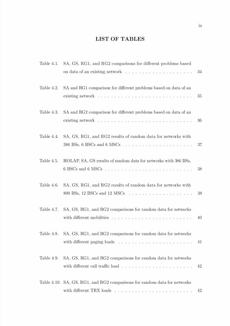
LIST OF TABLES
Table 4.1. SA, GS, RG1, and RG2 comparisons for different problems based
on data of an existing network . . . . . . . . . . . . . . . . . . . . 34
Table 4.2. SA and RG1 comparison for different problems based on data of an
existing network . . . . . . . . . . . . . . . . . . . . . . . . . . . . 35
Table 4.3. SA and RG2 comparison for different problems based on data of anexisting network . . . . . . . . . . . . . . . . . . . . . . . . . . . . 36
Table 4.4. SA, GS, RG1, and RG2 results of random data for networks with
386 BSs, 6 BSCs and 6 MSCs . . . . . . . . . . . . . . . . . . . . . 37
Table 4.5. HOLAP, SA, GS results of random data for networks with 386 BSs,
6 BSCs and 6 MSCs . . . . . . . . . . . . . . . . . . . . . . . . . . 38
Table 4.6. SA, GS, RG1, and RG2 results of random data for networks with
800 BSs, 12 BSCs and 12 MSCs . . . . . . . . . . . . . . . . . . . 38
Table 4.7. SA, GS, RG1, and RG2 comparisons for random data for networks
with different mobilities . . . . . . . . . . . . . . . . . . . . . . . . 40
Table 4.8. SA, GS, RG1, and RG2 comparisons for random data for networks
with different paging loads . . . . . . . . . . . . . . . . . . . . . . 41
Table 4.9. SA, GS, RG1, and RG2 comparisons for random data for networks
with different call traffic load . . . . . . . . . . . . . . . . . . . . . 42
Table 4.10. SA, GS, RG1, and RG2 comparisons for random data for networks
with different TRX loads . . . . . . . . . . . . . . . . . . . . . . . 42

8/6/2019 Location Area Paging
http://slidepdf.com/reader/full/location-area-paging 10/65
x
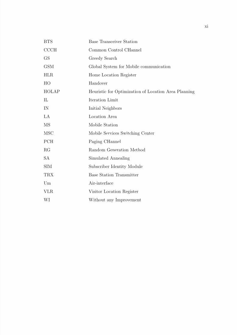
LIST OF SYMBOLS/ABBREVIATIONS
aij Proximity matrix element of BS i - BSC j
b jk Proximity matrix element of BSC j - MSC k
ci Call traffic of cell i at busy hour
C BSC j Call traffic capacity of BSC j
C MSC k Call traffic capacity of MSC k
di Peak call attempt rate of cell i per unit time
dij Matrix element of residence of i
th
BS and j
th
BS in same LADBSC j Busy Hour Call Attempt (BHCA) capacity of BSC j
DMSC k Busy Hour Call Attempt (BHCA) capacity of MSC k
hij Handover rate from ith cell to jth
lin LA-BS topology matrix of ith BS and nth LA
P BS i Paging capacity of BS i
P BSC j Paging capacity of BSC j
ri
Number of TRXs for each cell i
RBSC j TRX capacity constraint of BSC j
RMSC j TRX capacity constraint of MSC k
y jk BSC-MSC topology matrix of jth BSC and kth MSC
xij BS-BSC topology matrix of ith BS and jth BSC
α Temperature decrement rate of SA cooling schedule
λi Paging rate of cell i
λ∗i Total paging load in the LA of BS i
σ Standard deviation
AD Accepted to Decrease
BHCA Busy Hour Call Attempt
BS Base Station
BSC Base Sstation Controller
BSS Base Station Subsystem
8/6/2019 Location Area Paging
http://slidepdf.com/reader/full/location-area-paging 11/65
xi
BTS Base Transceiver Station
CCCH Common Control CHannel
GS Greedy Search
GSM Global System for Mobile communication
HLR Home Location Register
HO Handover
HOLAP Heuristic for Optimization of Location Area Planning
IL Iteration Limit
IN Initial Neighbors
LA Location AreaMS Mobile Station
MSC Mobile Services Switching Center
PCH Paging CHannel
RG Random Generation Method
SA Simulated Annealing
SIM Subscriber Identity Module
TRX Base Station TransmitterUm Air-interface
VLR Visitor Location Register
WI Without any Improvement

8/6/2019 Location Area Paging
http://slidepdf.com/reader/full/location-area-paging 12/65
1
1. INTRODUCTION
In cellular communication systems, on the arrival of a mobile-terminated call, the
system tries to find the mobile terminal by searching it among a set of base stations
(BSs) using the current region knowledge of the mobile. This search is called paging,
and the set of base stations in which a mobile is paged is called the Location Area (LA).
At each LA boundary crossing, mobile terminals register their new location through
signalling in order to update the location management databases. Therefore, the size
of the LA is important for reducing the cost of paging and registration signalling [1].Although there may be events other than location updates that cause registration, we
will use the term “registration” instead of “location update” throughout this document.
Considering the procedures of paging or registration, it can be seen that the
costs they produce have three different types of bases. One of them is the select or
update queries which create processing and storage load on the database elements of
the cellular network. The other one is the load created on the physical connection part
of the cellular network. The last one is the load on the air interface of the cellular
network. Among these, the least scalable one (which means as the population and
traffic in a cell grows, the most affected resource) is the radio bandwidth resource. In
addition, because the radio bandwidth is shared by those control functions like paging,
registration and call traffic, it is considered to be the scarcest resource in a wireless
network. Therefore, for paging and registration signalling costs, instead of considering
all types of costs, we may just take the cost of the load on the radio bandwidth into
account. It is desirable to design wireless networks that make efficient use of the limited
radio bandwidth. Use of effective mobility management schemes is needed to achieve
such efficiency [2].
1.1. GSM Network Design Considering Location Area Management
A GSM network comprises several elements: the mobile station (MS), the sub-
scriber identity module (SIM), the base transceiver station (BTS), the base station

8/6/2019 Location Area Paging
http://slidepdf.com/reader/full/location-area-paging 13/65
2
Figure 1.1. General architecture of a GSM network
controller (BSC), the mobile services switching center (MSC), the home location reg-
ister (HLR), and the visitor location register (VLR). Figure 1.1 provides an overview
of the GSM subsystems [3].
GSM network contains as many MSs as possible, available in various styles and
power classes. In particular, the handheld and portable stations need to be distin-
guished. GSM distinguishes between the identity of the subscriber and that of the
mobile equipment. The SIM determines the directory number and the calls billed to a
subscriber. The SIM is a database on the user side. Physically, it consists of a chip,
which the user must insert into the GSM telephone before it can be used: To make
its handling easier, the SIM has the format of a credit card or is inserted as a plug-in
SIM. The SIM communicates directly with the VLR and indirectly with the HLR.
BTSs take care of the radio-related tasks and provide the connectivity between
the network and the mobile station via the Air-interface (Um). The BTSs of an area
(e.g., the size of a medium-size town) are connected to the BSC via an interface called
the Abis-interface. The BSC takes care of all the central functions and the control of
the subsystem, referred to as the base station subsystem (BSS). The BSS comprises
the BSC itself and the connected BTSs. A large number of BSCs are connected to

8/6/2019 Location Area Paging
http://slidepdf.com/reader/full/location-area-paging 14/65
3
the MSC via the A-interface. The MSC is very similar to a regular digital telephone
exchange and is accessed by external networks exactly the same way. The major
tasks of an MSC are the routing of incoming and outgoing calls and the assignment of user channels on the A-interface. The MSC is only one subcenter of a GSM network.
Another subcenter is the HLR, a repository that stores the data of a large number of
subscribers. An HLR can be regarded as a large database that administers the data
of literally millions of subscribers. Every GSM network requires at least one HLR.
The VLR was devised so that the HLR would not be overloaded with inquiries on
data about its subscribers. Like the HLR, a VLR contains subscriber data, but only
part of the data in the HLR and only while the particular subscriber roams in thearea for which the VLR is responsible. When the subscriber moves out of the VLR
area, the HLR requests removal of the data related to a subscriber from the VLR. The
geographic area of the VLR consists of the total area covered by those BTSs that are
related to the MSCs for which the VLR provides its services [4].
In a mobile communication system, on the arrival of an incoming call to a wireless
customer, the system sets about finding the customer’s mobile terminal by searching
it among different base stations following a strategy dictated by the current knowledge
of the mobile. This search is called paging. The set of base stations in which a mobile
is paged when an arriving call needs to be routed is the location area. One or more
LAs may be served by a single VLR.
The current location area knowledge of a mobile is maintained by a registration
procedure in which mobiles announce their presence upon entering a new location area.
The new location area will be stored in some database to be used for paging the mobile
next time the mobile receives an incoming call. The size of the location area plays
an important role in cellular networks because of the trade-off caused by paging and
registration signalling.
When a Mobile Station (MS) is paged, a paging message is sent from the MSC
to each Base Station Controller (BSC) belonging to that MSC’s service area (global
paging ), or to those BSCs serving at least one cell belonging to the LA where the

8/6/2019 Location Area Paging
http://slidepdf.com/reader/full/location-area-paging 15/65
4
MS is registered (local paging ). For each paging message received by the BSC, Paging
Command messages have to be sent to all cells belonging to the LA where the target
MS is registered. The number of cells in an LA ranges from a few tens up to perhapsone hundred cells, sometimes even more. That means, one incoming paging message
to the BSC leads to a considerably larger number of outgoing paging commands from
the BSC.
Base Transceiver Station (BTS) has to broadcast all the incoming pages. The
paging request messages are sent on the Paging CHannel (PCH) on the Common
Control CHannel (CCCH). Too large LAs may lead to a too high paging load in theBTS resulting in congestion and lost pages. Smaller LAs reduce the paging load in the
BTSs as well as in the BSCs. However, smaller LAs also mean a larger number of LA
border cells in the network. Each time an MS crosses the border between two LAs,
a location update is performed. The location updates affect the load on the signaling
subchannels, SDCCH, in the LA border cells.
1.2. Literature Survey
LA management in cellular networks’ literature can be classified by the used
location update and paging scheme. These schemes are categorized as zone-based, time-
based, movement-based, distance-based, profile-based and state-based schemes. In
zone-based location update schemes, LA boundaries are fixed and the same boundaries
are used for all mobiles’ registrations. Therefore, cells that will do the registration
is known in advance. GSM (Global System for Mobile communication) is a widely
used cellular networks standard that employs zone-based scheme with some additional
constraints [4]. Optimization of location area planning in zone-based schemes is not
widely studied compared to other schemes in the literature. Saraydar et al. investigated
zone-based schemes by aiming to optimize the LA borders [1, 2]. When the location
update is performed according to the time elapsed since the last location update, used
scheme is called time-based location update scheme [5]-[7]. Implementation of the
time-based location update schemes are simple, however redundant signalling may be
incurred when the system has low mobility because of numerous stationary mobiles. In

8/6/2019 Location Area Paging
http://slidepdf.com/reader/full/location-area-paging 16/65
5
that situation, to handle those unnecessary signalling, calculating the time threshold
value depending on the speed and call arrival rate of the mobile is proposed in [5].
In movement-based scheme [8]-[13], location update decision is made considering
the number of cell boundary crossings measured since the previous location update.
Distance-based schemes state that location update will be carried out when a mobile
terminal moves a threshold number of cells away from the cell in which the last location
update was performed [14]-[20]. According to [21], the distance-based location update
scheme produces the minimum signalling cost compared to movement-based and time-
based schemes. However, the implementation of distance measurement considering thecell topology is needed which is difficult to implement. Various researchers investigate
ways to simplify the implementation [18, 19]. Finally, in the profile-based scheme the
location update is performed according to specific criteria [22]-[28]. The criterion could
be the mobility behaviour of the mobile, or it could be the distribution of the mobile
terminated call arrivals.
Comparison of the schemes mentioned above are investigated in [21, 29, 30].
In [29], methods for evaluating the performances of different location management
schemes are also presented. In addition to location update scheme, problems of storing
and querying the location information of objects in mobile computing surveyed in [30].
Beside the schemes mentioned above, geography-based scheme is defined in [31]. The
research presents an intelligent paging scheme, which uses geographical information for
the paging of the target mobile terminal. Because the characteristic of the geography
influences the distribution of mobile users, the geographical background information is
considered to track the mobile users.
Not only in the cellular networks, but also in other wireless environments to keep
track of the mobiles is crucial for the continuity of the given services. Hence, location
management is an important issue that should be defined and implemented in most
wireless systems. For example, location management schemes for wireless IP networks
are proposed in [32, 33]. Wireless ATM [34, 35] and mobile satellite systems [36] are
other systems that need location management. However, as the user population and

8/6/2019 Location Area Paging
http://slidepdf.com/reader/full/location-area-paging 17/65
6
network size increases; storing, querying and the scalability of the location information
becomes an essential problem for the design of the wireless system [27],[37]-[40].
The evaluation of location management algorithms depends upon the underlying
mobility model. Therefore the chosen mobility model is important for the performance
of the investigated location update and paging scheme. Several researchers proposed
mobility models for studying the performance of location management schemes [41]-
[45].
In this study, we propose a solution for zone-based location update and paging
schemes. Nevertheless, in the subject of “LA management in cellular networks”, most
of the works in the literature have a common objective: Minimizing the total paging
and registration cost. This objective function requires addition of the paging cost and
the registration cost. However, these costs do not have comparable units. In order to
compensate this difficulty, previous researchers use some assumptions for the relative
values of these costs such as assuming one unit cost for each paging-event is equal
to 10 unit cost for each registration-event. These assumptions have the deficiency of
being the same throughout the whole network. In reality, the load (i.e., cost) of paging
and registration to the network varies from cell to cell. In order to avoid the difficulty
of summing these two types of costs, instead of trying to minimize both, we decided
to bound the paging cost and minimize the registration costs which still results in a
difficult combinatorial optimization problem. However, compared to “minimizing the
paging within acceptable registration capacities”, this goal is advantageous since paging
capacity is easier to quantify as a constraint as explained in Section 2. We propose an
SA algorithm and a heuristic algorithm for this problem in Section 3 and finally, we
present the results of the computational experiments in Section 4.

8/6/2019 Location Area Paging
http://slidepdf.com/reader/full/location-area-paging 18/65
7
2. FORMULATION OF THE LOCATION AREA
PLANNING PROBLEM
Although it can be any cellular network, the model used in this work complies
with the Base Station (BS), Base Station Controllers (BSC), and Mobile Switching
Center (MSC) hierarchy of the cellular GSM networks. While formulating the LA
planning problem, we only use the available network information and try to include all
realistic constraints and goals. The overall problem in LA planning and dimensioning
is due to the tradeoff between the paging cost and the registration cost. The paging
cost is a result of the arriving calls to mobiles (i.e., mobile-terminated calls). The called
party has to be searched and found in order to establish the connection. In order to
have a feasible cellular network, we should not exceed the paging capacities of BS i and
BSC j (P BS i and P BSC j respectively). For evaluation of the paging loads, the paging
rate per unit time for each cell i , λi, is used. This paging rate of cell i (λi) just includes
the paging generated because of the mobiles residing in that cell.
The maximum call traffic load capacities of BSC j and MSC k (C BSC j and C MSC k
respectively) are other constraints that should be obeyed. These constraints are related
to the equipment used. To check those constraints, call traffic of each cell at busy hour
is used, which is shown as ci for cell i .
In order to have a feasible cellular network, the limited call processing capability
of MSCs and BSCs may create a limit on the peak call arrival rate (this call arrivalrate includes not only established connections but also the failed attempts). This limit
is called the Busy Hour Call Attempt (BHCA) capacity. This capacity for BSC j and
MSC k are represented as DBSC j and DMSC
k , respectively. The BHCA load on BSCs
and MSCs are calculated by using the call attempt rate of the cells. di denotes the
peak call attempt rate of cell i per unit time.
Each BS has a finite number of Transmitters (TRXs) which defines the numberof channels used in that cell. TRX capacity constraint is a vendor specific constraint
8/6/2019 Location Area Paging
http://slidepdf.com/reader/full/location-area-paging 19/65
8
of BSCs and MSCs. For each BSC j and MSC k , the sum of the number of TRXs for
each cell connected to that BSC or MSC should comply with a limit. These limits are
denoted as RBSC
j and RMSC
k , respectively. In order to check this constraint, we needthe number of TRXs for each cell i (ri).
For the registration load calculation, the required data is “idle” (i.e., with handset
on but not in a conversation) mobile flow rate between each cell pair. Since this data
generally cannot be collected, we approximate this aggregate mobile flow behavior by
assuming that the mobile flow rate between any given two cells is proportional to the
handover rate between these cells. In other words, handover traffic between each cellpair (i,s), his: handover rate from ith cell to sth cell is used instead of the mobile flow
data.
To propose a BS-BSC topology, we must know which BS can be connected to
which BSC and discard those BS-BSC pairs that are not feasible (due to physical
limitations, geographical constraints, etc.). This information is available in the form of
a proximity matrix, A, among BS and BSCs in which aij = 1 if BS i can be connected
to BSC j, and aij = 0 otherwise. In a similar way, for BSC-MSC topology, we will
use a proximity matrix, B , among BSC and MSCs in which b jk = 1 if BSC j may be
connected to MSC k, and b jk = 0 otherwise.
In addition to these, the following design variables will be used in the formulation:
LA-BS topology is represented with a matrix L in which:
If ith BS resides in nth LA then lin = 1, otherwise lin = 0.
L matrix is used to establish another matrix D in which:
If ith BS and sth BS resides in different LAs then dis = 1, otherwise dis = 0.

8/6/2019 Location Area Paging
http://slidepdf.com/reader/full/location-area-paging 20/65
9
BSC - MSC topology is represented with a matrix Y in which:
If jth
BSC connected to kth
MSC then y jk = 1, otherwise y jk = 0.
BS - BSC topology is represented with a matrix X in which:
If ith BS connected to jth BSC then xij = 1, otherwise xij = 0.
Paging cost on a cell is determined by the total call arrivals to cells that belong
to the same LA. Therefore, we use a vector, λ∗, in which, ith entry holds that total
value for ith cell. This value can be calculated as:
λ∗i = λi +
s
λs(1 − dis) (2.1)
As a result, our “Minimize the total registration signalling” goal is formulated as:
Minimizeis
dis
.his
(2.2)
which is subject to the following constraints:
Each BS should be assigned to exactly one BSC. So, for ith cell, BS-BSC topology
matrix should have only one entry in the ith row that has value 1 and others must be
0:
j
xij = 1 , ∀i (2.3)
Each BSC should be assigned to exactly one MSC. So, for jth BSC, BSC-MSC topology
matrix should have only one entry in the jth row that has value 1 and others must be
0:
k y jk = 1 ,
∀ j (2.4)

8/6/2019 Location Area Paging
http://slidepdf.com/reader/full/location-area-paging 21/65
10
Each BS should be assigned to exactly one LA. So, for the ith cell, BS-LA topology
matrix should have only one entry in the ith row that has value 1 and others must be
0:
n
lin = 1 , ∀i (2.5)
Each LA must reside within exactly one MSC. So, for each cell pairs, if they belong to
the same LA, then they also must belong to the same MSC:
If
n lin.lsn = 1 , then
k( j xij.y jk .
r xsr.yrk) = 1 , ∀(i, s)
Paging capacity of each BS must not be exceeded:
λ∗i < P BS i , ∀i (2.6)
Paging capacity of each BSC must not be exceeded. Assuming that BSC pages the MS
(Mobile Station) separately in each cell of the same LA, this constraint becomes:
i
xij .λ∗i < P BSC j , ∀ j (2.7)
Call traffic capacity of each BSC must not be exceeded:
i
xij.ci < C BSC j , ∀ j (2.8)
Call traffic capacity of each MSC must not be exceeded:
j
i
xij .y jk .ci < C MSC k , ∀k (2.9)
BHCA capacity of each BSC must not be exceeded:
i xij.di < D
BSC
j , ∀ j (2.10)

8/6/2019 Location Area Paging
http://slidepdf.com/reader/full/location-area-paging 22/65
11
BHCA capacity of each MSC must not be exceeded:
j
i xij .y jk .di < D
MSC
k , ∀k (2.11)
TRX capacity of each BSC must not be exceeded:
i
xij .ri < RBSC j , ∀ j (2.12)
TRX capacity of each MSC must not be exceeded:
j
i
xij.y jk .ri < RMSC k , ∀k (2.13)
Proximity constraints for BS-BSC connections are satisfied:
xij ≤ aij ,∀(i, j) (2.14)
Proximity constraints for BSC-MSC connections are satisfied:
y jk ≤ b jk ,∀( j,k) (2.15)
The general LA planning problem formulated in Equations 2.1 through 2.15 is a difficult
optimization problem in which LA-BS topology (the matrix L), BSC-MSC topology
(the matrix Y ), and BS-BSC topology (the matrix X ) have to be decided. There may
be many special cases of the general LA planning problem. In a typical case, some
of the constraints may be omitted. For example, there may not be any call capacity
constraint for MSCs, in that case Constraint (2.9) will be omitted. Another special
case is that there may be exactly one BSC for each MSC. In that special case, Y matrix
will be already known and is not needed to be decided.
There are also site constraints, which should be satisfied if the cellular network
is GSM. Those constraints are described as cells belonging to the same site must be

8/6/2019 Location Area Paging
http://slidepdf.com/reader/full/location-area-paging 23/65
12
connected to same BSC. This constraint is handled as follows: Sites are treated as
combination cells. Cells belonging to the same site can be grouped together to form
the combination cell whose loads are the summation of sub-cell loads. Summation of TRX, call traffic, BHCA and paging loads are required, since when all cells of a site
are connected to a BSC or assigned to an LA, they create that amount of load. Site
constraints are optional and considered in the solution techniques.

8/6/2019 Location Area Paging
http://slidepdf.com/reader/full/location-area-paging 24/65
13
3. SOLUTION TECHNIQUES PROPOSED
Our aim is to propose an algorithm that will take the available constraints, ca-
pacity and load information described in Chapter 2 as inputs, and find an optimal
or near optimal solution as a network topology which includes the assignment of cells
(BSs) to switches (BSCs and MSCs) and cells to location areas (LAs).
Since our solution space consists of all of the possible network topologies, the
determining factors of the solution space size are BS to BSC assignments, BSC to
MSC assignments, and BS to LA assignments. If we have n BSs, m BSCs, p MSCs,
the number of possible BS-BSC assignments is calculated as follows: for each BSs
there are m possible BSCs to be connected, hence we have nm possible connections.
Likewise number of possible BSC-MSC assignments is m p and because upper limit of
the number of LAs is the number of BSs (n ), the number of possible BS-LA assignments
are nn. Consequently the size of the solution space is found to be nm.m p.nn. Although
the solution space includes both feasible and infeasible solutions, we should assess all
solutions whether they are feasible or not. Because of the solution space size, exhaustive
methods would result in exponential time complexity.
The “bin packing” problem is previously shown to be NP-hard, i.e., there is no op-
timization technique that solves “bin packing” problem in polynomial time complexity.
Our sub-problem of assigning BSs to LAs can be mapped to the bin packing problem
in the following way: LAs correspond to bins due to their common paging capacity
limit. We try to pack the BSs to LAs in such a way that we need the minimum number
of LAs. This minimization of the number of LAs is a step in the minimization of the
cost of the resulting network. Since only a sub-component of the optimization prob-
lem is NP-hard, as a consequence the overall optimization problem can be classified as
NP-hard.
Since our problem is a difficult optimization problem, it is not possible to guar-
antee finding the optimal solution in reasonable running times. Therefore, other tech-

8/6/2019 Location Area Paging
http://slidepdf.com/reader/full/location-area-paging 25/65
14
niques that give near optimal solutions within acceptable run times are needed. One
of the methods that find a sub-optimal solution without searching the whole solution
space is simulated annealing (SA). SA was introduced by Metropolis et al. [46] andis used to approximate the solution of very large combinatorial optimization problems
[47]. Beside the traditional greedy local search techniques, the stochastic properties
of the SA algorithm prevent it to get stuck to local minima. On the other hand, in
traditional greedy local search, the quality of the final result heavily depends on the
initial solution. In contrast, the idea behind SA is to do enough exploration of the
whole solution space early on so that the final solution is insensitive to the starting
state [48]. Detailed information about SA algorithm could be found in [49]. Beside,application of SA algorithm on different research subjects are illustrated in [50]-[53].
The information supplied to the SA based algorithm includes the BHCA, call
and TRX capacity constraints for BSCs and MSCs; paging capacity constraints and
proximity data (allowed connections to MSCs and BSCs, respectively) for BSCs and
BSs. Moreover, information related with the call traffic for each BS is also supplied.
This cell traffic and the capacity information include the Peak Call Attempt Rate,
Peak Call Traffic Rate, Paging Rate, Handover Rate to Neighbor BSs, and Number
of TRX attached. Although these load values could be generated using any mobility
model, they could be fetched from an existing network.
The SA based algorithm described here finds a network topology that consists of
LA-BS assignment (the matrix L), BSC-MSC topology (the matrix Y ), and BS-BSC
topology (the matrix X ). Moreover, the total registration cost of the solution found is
also presented.
The algorithm starts with an initial feasible solution, which is set as our current
solution. Randomly a neighbor solution from the solution space is chosen and its cost
is compared to the current solution’s cost. If that neighbor is improving the cost, it
is accepted directly and that neighbor solution is set as the current solution. If the
neighbor does not improve the cost, then this solution is accepted with a probability
that is calculated according to the stage the algorithm is in (we designate this stage

8/6/2019 Location Area Paging
http://slidepdf.com/reader/full/location-area-paging 26/65
15
via a variable called “temperature”). The probability of accepting a worse solution is
[47]:
P = e−∆E/T (3.1)
where ∆E is the difference between the costs of the neighbor solution and the current
solution. The value of the temperature is managed by the cooling schedule that controls
the execution of the algorithm.
For a successful SA implementation, two key items that must be defined carefullyare the moves that create neighbor solutions and the cooling schedule. Appendix A
contains pseudo code of the SA algorithm. In Subsection 3.1, neighborhood structure
and the cooling schedule implemented are described.
3.1. Simulated Annealing
3.1.1. Neighborhood Structure
A feasible solution is a topology that all network nodes (BSs, BSCs, MSCs) are
connected and the LA borders are specified while satisfying the constraints. Therefore,
a (feasible) neighbor solution may be generated by any of the three types of moves:
• Changing a BS to BSC assignment: A BS to be moved is randomly chosen,
and then a BSC is randomly chosen among all BSCs in the proximity of thatBS. Before doing that move, the capacity constraints affected by this BS-BSC
connection are checked. If these constraints are not violated, the new BSC is
assigned to the BS. Then, a random feasible LA is searched to assign that BS
among the existing LAs residing in the new BSC. Because of the limitation that
an LA could not spread over MSCs, instead of checking whether the new BSC
and the old BSC are connected to the same MSC, we directly try to find an LA
residing in the new BSC. If no feasible LA is found which means that we need a
new LA for the new BSC and that LA is created. Then, all load updates resulting

8/6/2019 Location Area Paging
http://slidepdf.com/reader/full/location-area-paging 27/65
16
from that move are calculated on the network.
• Changing a BSC to MSC assignment: This move results in a big change in the
network topology, since all BSs connected to that BSC also move with it. First,a BSC is chosen randomly to change its MSC connection. The candidate MSC
is also randomly chosen among all MSCs. Again before doing that move, the
capacity and proximity constraints of that BSC-MSC connection are checked. If
these constraints are not violated, the new MSC is assigned to the BSC. LAs
residing merely in that BSC (i.e., none of their BSs are connected to another
BSC) stay with their BS connections (i.e., nothing is changed for these LAs),
but LAs having some of their BSs connected to that BSC goes under some re-arrangement. The assignments of BSs to those LAs are released, and therefore
those LAs have no more BSs assigned to them from that BSC. Moreover, for those
“released” BSs, an adequate amount of new LAs are created (if the capacity of a
new LA is full, then another LA is created).
• Changing a BS to LA assignment: Without affecting the BS-BSC connection, a
new LA assignment is done by searching the available LAs residing within the
same BSC. First a BS is chosen randomly to change its LA assignment. Thencandidate LA is randomly chosen among all the LAs residing within the connected
BSC. After the capacity constraint of LA-BS connection checking, the new LA is
assigned to the BS.
When a new neighbor is to be created, type of the move to be made is chosen.
Although there are three kinds of moves, they do not change the network architecture
in similar ways. For example, a change in BSC-MSC connection may have a largeimpact on the cost of the network. Therefore, choice of the move type to be made
is not uniformly distributed between these three types. The move types are chosen
according to some probabilities assigned for each type. These probabilities have an
impact on the performance of the SA algorithm. The effect of different probability
assignments on the quality of results, and the computation time could be investigated.

8/6/2019 Location Area Paging
http://slidepdf.com/reader/full/location-area-paging 28/65
17
3.1.2. Cooling Schedule
The cooling schedule consists of three important components: setting the initialtemperature, the decision of when and how to decrease the temperature, and the
decision of when to stop the algorithm. Among different cooling schedules, the most
efficient ones may be found by trying different cooling schedules and observing the
effect on both the quality of the solution that is found and the rate at which the
process converges [54].
The initial temperature calculation is important, because if the initial tempera-
ture is too high then the time to reach the result increases very much. On the other
hand, if the initial temperature is taken too small then the algorithm will not have the
freedom of making enough random moves to visit different local minima and stay in a
relatively deeper one. As a result, the final result may depend on the initial topology
[55]. The idea is that at the initial stage of the algorithm, nearly all neighbors should
be accepted. In other words the initial probability of accepting a worse solution (P 0)
should be very close to 1, such as P 0 = 0.999. We set our initial temperature (T 0) to
achieve that probability at first stages by using formula (3.1). Extracting T from that
formula yield us:
T 0 =−max ∆E
ln P 0(3.2)
In order to obtain the maximum possible cost difference between the neighbor solu-
tions, max ∆E in equation (3.2), a predefined number of neighbors starting with the
initial solution is created and the maximum difference between the costs of each of the
neighbors. The reason of using the maximum cost change is to be able to start with a
system that accepts any neighbors with probability P 0.
Whenever, a certain number of new solutions are accepted, the temperature is
decreased according to the following formula:
T new = T old ∗ α (3.3)

8/6/2019 Location Area Paging
http://slidepdf.com/reader/full/location-area-paging 29/65
18
The cooling factor, α, effects the quality of solutions and the run times significantly.
Typical values of α lie between 0.85 and 1.
Towards the end of the algorithm, the temperature goes towards zero and it
becomes difficult to accept new topologies. For that reason, we have another criteria for
the decision of when the temperature should be decreased. At a specific temperature, if
the total number of neighbors tested (not just the accepted ones) reaches approximately
to the neighborhood size, then the temperature is decreased using Equation 3.3 again.
This neighborhood size in our implementation is considered to be roughly equal to the
multiplication of the number of BSs, BSCs, and MSCs in the network. Since, at aspecific topology, you almost have that many possible neighbor solutions.
The algorithm must stop if it cannot find better solutions anymore. In our imple-
mentation, the SA algorithm stops if we cannot accept new solutions in a predefined
number of temperature decrements. Again, this stopping criterion affects significantly
the quality of results and the execution time of the algorithm. In order to guarantee
a finite run-time implementation, the SA search is also stopped if a very large number
of solutions are tried. During the SA search “the best solution so far” is recorded and
presented when the algorithm stops. Because performance of SA depends heavily on
the mentioned two key items (Cooling Schedule and Neighborhood Structure), these
items should be carefully investigated and optimized to have the best results. Details
of the optimization method and the resulting cooling schedule settings are described
in the Chapter 4.2 which are published as [56].
3.2. Greedy Search
As a natural competitor, Greedy Search (GS) is one of the techniques that we
compare our SA based algorithm. It starts with a feasible random solution. Among
feasible neighbors, one is selected randomly. If the chosen neighbor improves the cost
of the current solution then it is accepted as the current solution. The search continues
until an “iteration limit” is reached or a “specified number of iteration” results in no
improvement.

8/6/2019 Location Area Paging
http://slidepdf.com/reader/full/location-area-paging 30/65
19
Results of GS should form an upper bound for the SA runs, since the greedy
search can only find the local minima of the solution space. However, the quality of
the GS result heavily depends on the initially formed solution. Therefore a number of runs performed to test the GS with different initial solutions. Extracted information
from the GS runs is the resulting network topologies and the cost of the networks.
3.3. Heuristics
For optimization problems, an alternative solution method is using heuristic al-
gorithms. Although the quality of the heuristic algorithm results could be worse thanother solution techniques, it would be preferred because of its time complexity. Since
that method tries to find the best solution without tracing an extensive part of the
solution space, and instead it attempts to build the best solution directly, its time
complexity is generally much better than other solution techniques.
The cost of the cellular network was designated by the sum of the number of
handovers among cells belonging to different LAs, since those handovers were assumed
to be proportional to the number of location updates done by crossing the LA borders.
The minimization of the total network cost could be achieved by setting the LA borders
such that the cell pairs belonging to different LAs have the smallest handover values.
The heuristic proposed in this thesis is named HOLAP (Heuristic for Optimization
of Location Area Planning). It is based on the decision described above. Hence, the
most important goal of the HOLAP is to gather cell pairs with high handovers within
the same LA, so that the cost of the network is not raised by those high handover
values. HOLAP algorithm has two main blocks. Figure 3.1 and Figure 3.2 represent
the flow diagrams of these blocks. As the first figure describes, the algorithm starts
with sorting the cell pairs according to the handover rate between the pair. The cell
pair that is being processed is checked for the previous LA assignments and if there is
an LA assignment done to any of the cells in the pair, that pair is discarded.
Starting with the pair that induces the highest handover rate, algorithm tries to
8/6/2019 Location Area Paging
http://slidepdf.com/reader/full/location-area-paging 31/65
20
assign a common LA to both cells of that pair. Assignment process begins by searching
feasible BSCs for that pair. Feasibility check is done by assuring that capacities of the
BSC are enough to handle these cell-to-BSC assignments. If the number of availableLAs is more than one, then the decision of the LA assignment is made according to
decision priorities shown in the flow diagram. After the processing of all cell pairs in
a sequential manner, there will be cells that are not assigned to any LA. For these
remaining unassigned cells, the algorithm described in the Figure 3.2 is applied. Again
the decision priorities are considered.

8/6/2019 Location Area Paging
http://slidepdf.com/reader/full/location-area-paging 32/65
21
Figure 3.1. Flowchart of HOLAP

8/6/2019 Location Area Paging
http://slidepdf.com/reader/full/location-area-paging 33/65
22
Figure 3.2. Flowchart of HOLAP (cont’d)

8/6/2019 Location Area Paging
http://slidepdf.com/reader/full/location-area-paging 34/65
23
4. COMPUTATIONAL EXPERIMENTS
The cluster system named “ASMA” (Advanced System for Multicomputer Appli-
cations) is used for experiments. ASMA resides in Computer Engineering Department
of Bogazici University, and has 32 PCs with Linux operating system [57]. The exe-
cution time varies with the size of the problem and SA parameters used, but so far
the longest run has taken about 1.5 hours for our reference case. In order to find
the SA parameter values that give the best result, the first group of experiments is
performed using different parameter values on different data sets. Experiments arerepeated approximately 30 times for each data and parameter set. The data sets used
in the experiments are obtained from a GSM network. These data sets are formed
by collecting data from the GSM network at different times of a week. By choosing a
pilot area from the GSM network, the information about the network elements (BS,
BSC, and MSCs) is extracted. Number of these network elements defines the size of
the problem.
In the second and third group of experiments, different solution techniques are
applied to the same data sets. The performance of the proposed SA technique is
compared with the results of these solution techniques. The compared techniques
are greedy search (with random initial topology), random generation, and the heuristic
algorithm. Comparison of SA with other evolutionary algorithms for different problems
could be found in [58, 59].
4.1. Implementation of the Algorithms
Algorithms are implemented by using C++ programming language, because of
its modularity and flexibility. The GSM network elements (cells, BSCs, and MSCs)
have a number of shared attributes such as call traffic load and TRX load. Therefore
a common base class is defined, namely ‘NwElement’, and all other network element
classes (MSC, BSC, BS) are inherited from that base class. NwElement class has the
following attributes:
8/6/2019 Location Area Paging
http://slidepdf.com/reader/full/location-area-paging 35/65
24
• id(integer) : Distinguishing ‘id’ number of the network element
• name(string) : Name of the network element
• pagingCap(floating number) : Paging capacity of the element• pagingLoad(floating number) : Number of paging command per second
• callTraffCap(floating number) : Call traffic capacity (in Erlangs)
• callTraffLoad(floating number) : Call traffic load (in Erlangs)
• BHCA Cap(integer) : Busy Hour Call Attempt Capacity
• BHCA Load(integer) : Total “Busy Hour Call Attempt” load of all connected
cells
• TrxCap(integer) : Limit of total connected cells’ TRX number• TrxLoad(integer) : Total number of TRX of connected cells
• proximity(array of proximity structure) : Holds proximity data
• connectedUp(pointer) : Points connected MSC for BSCs; points connected BSC
for BSs.
• connectedDown(array of pointers) : Holds pointers to connected BSCs(BSs) for
MSC(BSC).
Beside the classes mentioned above, an LA class representing LAs and a GSM-
Netwok class to be used for holding network topologies are defined. Figure 4.1 shows a
network representation with instances of these classes. For BS, BSC, and MSC classes,
although all attributes are inherited from ‘NwElement’ class, the ones written in italic
in Figure 4.1 are not used since those capacity limits do not exist for those elements.
Finally a SimAnnealing class is used for handling the execution of SA algorithm,a Heuristic class is used for implementation of the HOLAP , and a randomNW class is
used for creating random network data according to some input parameters.
While executing algorithms, our program updates all load attributes of the net-
work elements. By using this data, the average utilization of capacities are output to
files for the resulting network at the end of the program. If desired, the load on any
network element, or its utilization can also be queried.
8/6/2019 Location Area Paging
http://slidepdf.com/reader/full/location-area-paging 36/65
25
Figure 4.1. Representation of a GSM network via C++ classes

8/6/2019 Location Area Paging
http://slidepdf.com/reader/full/location-area-paging 37/65
26
4.2. Simulated Annealing Based Solution Technique
4.2.1. Typical Run of SA Algorithm
Figure 4.2 shows the cost of the solutions found at different stages of a typical
SA run for a moderate sized example network. This network had about 600 BSs, 6
BSCs and 6 MSCs. The parameter optimization of the SA algorithm is done with
that network and verified with other example networks. At the initial stages, since
the temperature is very high, the SA algorithm accepts nearly all solutions. It acts as
random search first, and the cost of the accepted solutions changes in a wide range asseen in Figure 4.2. As the temperature decreases, the probability of accepting worse
solutions also decreases. Because of that, at later stages of the run, the search becomes
greedy and only better solutions are accepted.
0 0.5 1 1.5 2 2.5 3
x 104
0.5
1
1.5
2
2.5
3
3.5
x 104
Iteration Number
N e t w o r k C o s t
Figure 4.2. A typical run of the SA algorithm on an example network

8/6/2019 Location Area Paging
http://slidepdf.com/reader/full/location-area-paging 38/65
27
4.2.2. Effect of SA Parameters
As seen from the pseudo-code of the SA algorithm presented in Appendix A, ex-ecution of the algorithm depends on a number of parameters. The first SA parameter
mentioned in the pseudo-code is the number of neighbors generated (IN: Initial Neigh-
bors) starting with the initial solution to calculate the initial temperature according to
the formula (3.2) using cost differences of the neighbors. This parameter affects only
the initial temperature, since the larger the number of neighbors traced is the greater
the possibility finding higher cost differences between two neighbors and hence, higher
the initial temperature as seen in Figure 4.3. Therefore to be able to start in a hotsystem (a system accepting nearly every neighbor solution), this parameter should be
set to a high value like 10,000.
25 2500 40000 1000000
1
2
3
4
5
6
7x 10
7
Number of initial neighbors (IN)
I n i t i a l T e m p e r a t u r e
Min
Mean
Max
Figure 4.3. Effect of SA parameters: IN
The second parameter used in SA algorithm is the value of alpha ( α) used to
decrease the temperature of the system as in formula (3.3). The higher its value, the
slower the system cools down. The range of α was between 0.9 and 1. By setting thisalpha value high, larger portion of the solution space can be searched, but run time

8/6/2019 Location Area Paging
http://slidepdf.com/reader/full/location-area-paging 39/65
28
gets longer. Figure 4.4 states that value 0.9999 performs better compared to the values
0.99, and 0.999.
0.99 0.999 0.99990
1
2
3
4
5
6
7
8x 10
5
Alpha
R e s u l t i n
g N e t w o r k C o s t
Min
Mean
Max
Figure 4.4. Effect of SA parameters: Alpha
Number of accepted solutions to decrease the temperature (AD: Accepted to
Decrease) is the third parameter used. If this value is small, then the SA algorithm
converges faster. Values assigned to this parameter had a range from 10 to 30 in
our experiments. As Figure 4.5 denotes, although the value of AD does not have much
effect on the quality of results, the value 20 gives slightly better results than the others.
A run is ended if after a specified number of temperature decrements are made
without any improvement in the cost (WI: Without any Improvement) or if number
of neighbors tested exceeds an iteration limit (IL: Iteration Limit). However, if you
stop the run in a system that is not cooled down enough, then you may miss better
solutions. Therefore, we took these parameters high enough so that results are able to
converge. Note that unnecessarily high value assignments, makes the run time of the
algorithm longer. WI should have a value near to 5,000 as seen from the Figure 4.6
and IL should have a value about 5,000,000 according to Figure 4.7.

8/6/2019 Location Area Paging
http://slidepdf.com/reader/full/location-area-paging 40/65
29
10 20 300
1
2
3
4
5
6
7x 10
5
Number of accepted solutions to decrease the temperature (AD)
R e s u l t i n g n e t w o r k c o s t
Min
Mean
Max
Figure 4.5. Effect of SA parameters: AD
5000 8000 100000
1
2
3
4
5
6
7x 10
5
Without any Improvement (WI)
R e s u l t i n
g N e t w o r k C o s t
Min
Mean
Max
Figure 4.6. Effect of SA parameters: WI

8/6/2019 Location Area Paging
http://slidepdf.com/reader/full/location-area-paging 41/65
30
2000000 5000000 8000000 100000000
1
2
3
4
5
6
7
8
9
10x 10
5
Iteration Limit (IL)
R e s u l t i n g N e t w o r k C o s t
Min
Mean
Max
Figure 4.7. Effect of SA parameters: IL
4.3. Statistical Quality Measurements
Beside of GS and Heuristics, a large set of randomly generated solutions is also
used to investigate the quality of SA results.
4.3.1. Random Generation Method 1 (RG1)
Because our solution space is huge, in order to have a feeling about the distribu-
tion of the cost values in the solution space, and to see how far from the average of the
solution space the SA results are, RG methods are used. RG methods are based on
the procedure that first BSs are connected randomly to feasible BSCs (considering the
constraints), and then BSCs are connected to feasible MSCs. Finally in RG1, for each
MSC starting with one LA, BSs are assigned to an LA. If LA capacity (paging capacity
of BSs) reaches to its limit, then a new LA is created and remaining BSs started to be
assigned to that LA. Here the aim is to create the minimum number of LAs for each
MSC (after randomly establishing BS-BSC-MSC topology).

8/6/2019 Location Area Paging
http://slidepdf.com/reader/full/location-area-paging 42/65
31
A histogram of the cost values found by the RG1 method for our reference case
can be seen in Figure 4.8. The histogram is established with approximately 27,000
random solutions. As it can be seen from the figure, the cost values have a normaldistribution.
1.8 2 2.2 2.4 2.6 2.8 3 3.2
x 106
0
200
400
600
800
1000
1200
1400
1600
Network Cost
F r e q u e n
c y
Figure 4.8. RG1 histogram
4.3.2. Random Generation Method 2 (RG2)
In RG2 method, for each MSC a random number of LAs are created. The ran-
domization is based on the uniform distribution with upper limit to be the number of
BSs connected to BSCs of the MSC. Then, all BSs are assigned to a random feasibleLA. If for a BS, no feasible LA exist then a new LA is created and the BS is assigned to
it. Here, the aim is to make all of the network topology decisions random and therefore
to simulate the solution space more accurately.
In RG2 method, because for each MSC a random number of LAs are created, the
total number of LAs created in the system deviates a lot from the minimum possible
number. For example, if the number of MSCs in a system is 6, then minimum numberof LAs that can be created is 6. For each MSC, LAs are created randomly, and the

8/6/2019 Location Area Paging
http://slidepdf.com/reader/full/location-area-paging 43/65
32
probability of having the number of LAs close to 6 is very small. This is the reason
of accumulation of the RG2 results to the right side of Figure 4.9. The histogram is
established with approximately 16,000 random solutions for our reference problem.
2.7 2.8 2.9 3 3.1 3.2 3.3 3.4 3.5
x 106
0
10
100
1000
10000
Network Cost
F r e
q u e n c y
Figure 4.9. RG2 histogram
4.4. Comparison of Solution Techniques
The comparison between SA and the other techniques are done based on the
resulting network costs found by them. First experiment group used data collected
from three selected pilot areas of an existing GSM network as the input given to the
algorithms. For the second group of experiments, random network data is generatedand instead of the real data that random input is used. The number of the BSs, BSCs
and the MSCs that will be built in the random network are taken as parameters. To
achieve the feasibility of the random data generated for those network elements, data
generation is done based on the average values of loads measured on the existing GSM
network. Loads of the network elements are assumed to be exponentially distributed
with the mean of the loads to be the average value measured on the existing GSM
network. Proximity matrices are set so that each BS could connect to each BSC andeach BSC could connect to each MSC. Data sets are formed with those generated

8/6/2019 Location Area Paging
http://slidepdf.com/reader/full/location-area-paging 44/65
33
loads and proximity matrices. The last group of experiments is performed to have
random data representing different type of a cellular network compared to the existing
one. This is done by changing the mean values of the exponential distributions. Forinstance, to represent a network with higher mobility subscribers, the mean value of
the handover rates is scaled up by three.
Comparisons are done by running the algorithms multiple times and taking the
average or the minimum values of the results. Therefore SA algorithm is applied to
each data set approximately 30 times and the mean of the multiple runs is calculated
for comparison. Beside, the minimum result found from the GS, RG1 and RG2 runsis selected for calculation. Number of GS algorithm runs on each data set is between
30 and 100. RG1 and RG2 methods are applied 10000 times to each data set.
4.5. First Group of Experiments
Based on the network data collected from an existing network, first group of
experiments yield us Table 4.1. The first data set is the data extracted from the first
pilot area of the existing network. Data sets numbered from two to five are extracted
from the second pilot area at different times of a week. Finally the sixth data set
is extracted from the third pilot area. As can be seen from Table 4.1, the SA based
solution technique outperformed the other methods. Besides, Table 4.1 shows that the
minimum of results found from RG2 runs is never lower than the minimum found from
the RG1 runs. That means setting number of LAs randomly and then making the
BS-BSC-MSC assignments could not give a better result than making BS-BSC-MSC
assignments randomly and then setting the number of LAs to the minimum possible
value. Other outcome of Table 4.1 is that SA gives approximately 50 per cent better
results than the GS method. This is an important value since the best competitor
method of SA investigated in this research is GS.
Although, just the mean value of the SA results is presented in Table 4.1, the
range of SA results found on different runs is not very large. For example, 30 separate
SA runs performed for Data Set 1 were ranging from 405,571 to 475,072. That means

8/6/2019 Location Area Paging
http://slidepdf.com/reader/full/location-area-paging 45/65
34
Table 4.1. SA, GS, RG1, and RG2 comparisons for different problems based on data
of an existing network
Data SA GS (Min) RG1 (Min) RG2 (Min)
Set1 450,882 792,769 1,870,809 2,772,498
Set2 12,161 24,693 134,410 161,974
Set3 15,352 27,930 138,889 161,365
Set4 11,514 20,839 109,852 131,300
Set5 7,308 14,910 84,571 101,962
Set6 901 1,956 22,402 31,508
the maximum and the minimum results found on distinct SA runs diverge at most 15
per cent from the average, which is an acceptable value. Therefore, we may state that
SA has a small range and any execution of the SA method gives results near to the
values presented in the tables.
To have an idea of how far the SA results are from the mean of the solution space,
RG methods are used. The process of creating a random network topology is achievedas follows: First, all BSs of a real GSM network are selected with their measured
load values, beside BSCs and MSCs of the GSM network are also selected but without
their load values. Then, each BS is randomly connected to a BSC while increasing the
loads of that BSC. Finally each BSC is connected to one of MSCs. Thus the resulting
network consists of real (measured) loads but an arbitrary topology.
The standard deviation can be used as the unit of distance from the mean value.
For the first group of experiments, the mean value of SA results are compared with the
mean and standard deviation(σ) of RG1 runs in Table 4.2. Data Sets 2 to 5 represented
in the first group of experiments contains measured data from the same area of a real
GSM network but at different days of a week. However, the loads obtained at peak
hours of these days are very different. That is why, significant differences are observed
between results found for these data sets.
The reason of high “RG1 (Min)” values compared to SA results could be the

8/6/2019 Location Area Paging
http://slidepdf.com/reader/full/location-area-paging 46/65
35
Table 4.2. SA and RG1 comparison for different problems based on data of an
existing network
Data SA RG1 (Mean) RG1(Std. Dev.)
Set1 450,882 2,572,020 156,555
Set2 12,161 150,569 3,220
Set3 15,352 153,915 3,305
Set4 11,514 122,772 2,493
Set5 7,308 94,253 1,845
Set6 901 29,937 1,692
number of RG1 executions, which is 10000. In spite of this, because RG1 histogram
shows the properties of a normal distribution, we may calculate the possibility of having
the value found by SA in that distribution using the mean and the standard deviation
of the RG1 histogram. For instance, in the case of the first data set the distance from
SA result to the mean of RG1 results is 13 σ.
Although the mean values of the fifth and the sixth data sets have 1/3 ratio,their standard deviations are found to be very near. The reason of that is, probably
because these data sets are based on the data measured from different GSM network
regions. Besides, when results for data sets 2 to 5 are compared, one can notice that
as the mean of RG1 decreases, the standard deviation of RG1 also decreases. This is
reasonable since these data sets are derived from the same region of a GSM network.
RG2 designates the actual solution space; however, it only includes the feasible
solutions. Finally for the first group of experiments, Table 4.3 shows the mean value
of SA results compared with the mean and standard deviation of RG2 runs. Since the
network topologies created by RG2 method are collected in a smaller region, RG2 has
smaller standard deviation compared to RG1. Hence, in the units of σ, the distance
of SA result to the RG2 mean is much more than the RG1. As an example, again
for the case of the second data set the distance from SA result to the mean of RG2
results is 48 σ. Number of RG2 method runs for each data set was 10000. The SA
- RG2(Mean) distance values may change as the number of runs performed for RG2

8/6/2019 Location Area Paging
http://slidepdf.com/reader/full/location-area-paging 47/65
36
Table 4.3. SA and RG2 comparison for different problems based on data of an
existing network
Data SA RG2 (Mean) RG2(Std. Dev.)
Set1 450,882 3,379,986 61,265
Set2 12,161 178,509 1,993
Set3 15,352 182,433 2,034
Set4 11,514 145,526 1,636
Set5 7,308 111,731 1,206
Set6 901 43,621 1,527
method increases. Another observation from Table 4.3 is that the first data set produces
much higher values compared to other data sets. The reason is that the first pilot area
is more extensive and condensed region.
Although the mean value found by RG2 method for Data Set 6 is smaller than
the other data sets, its standard deviation is very near to that of others. The reason
could be, as we mentioned earlier, the difference in the pilot area used for collectingreference data. Because, when Data Set 2 to 5 are investigated, a relation between
the mean and the standard deviation could be noticed. That is, considering the same
pilot area; as the mean value increases, the standard deviation also increases. Another
interesting observation is that for some of the data sets RG1 and RG2 methods have
close mean and standard deviation values. The mean value found at RG1 runs for
Data Set 2 is 150,569; however for the same data set the mean value of RG2 runs is
178,509. For Data Set 6, the standard deviations found for RG1 and RG2 methods are
1692 and 1527, respectively.
4.6. Second Group of Experiments
Random data generated based on the average values calculated from a GSM
network is used as input of the solution techniques. Table 4.4 lists the comparison of
the resulting network costs of these solution techniques for a network with 386 BSs, 6
BSCs and 6 MSCs. Although the loads are randomly generated for all elements based

8/6/2019 Location Area Paging
http://slidepdf.com/reader/full/location-area-paging 48/65
37
Table 4.4. SA, GS, RG1, and RG2 results of random data for networks with 386 BSs,
6 BSCs and 6 MSCs
Data SA GS (Min) RG1 (Min) RG2 (Min)
Set1 5,647 6,346 35,257 54,163
Set2 5,495 6,844 37,306 57,575
Set3 5,178 6,159 31,567 45,649
Set4 5,824 7,285 36,210 53,616
Set5 5,229 5,130 30,201 47,459
Set6 5,536 5,232 31,974 52,479
Set7 5,541 7,647 35,043 54,024Set8 5,265 8,289 36,925 54,223
Set9 5,626 6,520 36,927 55,071
Set10 5,548 6,509 32,331 61,336
on the mean values calculated using a real GSM network data, results obtained from
all methods are similar. As seen from Table 4.4, SA again found the best results beside
other methods. However, one notable discovery is that GS results are nearer to SA
results compared to runs performed with the real data. For the first data set SA is 11
per cent better than the GS result. This value was 43 per cent for the first data set in
Table 4.1. One explanation of this difference could be that loads generated according
to some specific distributions have similar values compared to real GSM network loads.
Hence for any solution, neighboring solutions would have similar costs, and it will be
harder for SA to find much better solutions.
Comparison of SA algorithm with the proposed heuristic algorithm(HOLAP ) is
shown in Table 4.5. The loads of the network elements are generated randomly again
based on the mean values obtained from a real GSM network. As seen from Table
4.5, HOLAP is not a competitor to SA, not even to GS method. The reason of the
worse results of HOLAP could be that the first pairs with higher handover rates are
considered and the pairs with low handover rates are discarded. Main aim is assigning
the pairs with high handover rates to the same LA. However then, remaining pairs had
to be assigned to different LAs due to system constraints. We know that the highest

8/6/2019 Location Area Paging
http://slidepdf.com/reader/full/location-area-paging 49/65
38
Table 4.5. HOLAP, SA, GS results of random data for networks with 386 BSs, 6
BSCs and 6 MSCs
Data HOLAP SA GS (Min)
Set1 21,682 4,932 7,806
Set2 21,605 4,565 9,027
Set3 21,417 4,387 5,557
Set4 20,723 4,820 9,236
Set5 21,389 4,368 5,476
Set6 22,288 4,628 5,232
Set7 23,214 4,365 6,145Set8 22,770 4,649 6,475
handover rates are not allowed to affect the network cost by grouping them in the
same LA. Therefore, it is obvious that remaining pairs are determining the network
cost, which means cell pairs with average or low valued handovers are also be important
for the network costs and should not be ignored.
Table 4.6 indicates the results of the solution techniques found for a random net-
work with 800 BSs, 12 BSCs and 12 MSCs. For the experiments conducted on this
larger network topology, data sets are obtained again by random data generation. As
seen in Table 4.6, SA has more reasonable results. It is interesting that even though
these values are obtained by using random data, acquired results are very close to the
results shown on the second,the third, and the fourth rows of Table 4.1. It should be
noticed that values of each column is similar among these tables. This similarity could
be a proof for the reliability of the random data generation.
Table 4.6. SA, GS, RG1, and RG2 results of random data for networks with 800 BSs,
12 BSCs and 12 MSCs
Data SA GS (Min) RG1 (Min) RG2 (Min)
Set1 13,807 27,725 106,844 126,409
Set2 14,122 29,409 110,059 131,725

8/6/2019 Location Area Paging
http://slidepdf.com/reader/full/location-area-paging 50/65
39
4.7. Third Group of Experiments
The average values calculated from a real GSM network are scaled up or downto obtain the example problems in this group. For a network with high mobility,
the mean value of the handover rates, which is obtained from the GSM network, is
multiplied by two and the other mean values are remained unchanged. For a network
with low mobility, the mean value is divided by two and the other mean values remained
unchanged. In Table 4.7, data sets from High1 to High4 have high mobility, and data
sets from Low1 to Low4 belong to networks with low mobility. For every remaining
table, data sets included represent a random network whose data formed by using thesame mean values. This is one of the reasons for the results of the table to be so close.
As seen in Table 4.7, an impact of high mobility is an increase in cost values. When
the table is compared to Table 4.4, this becomes more obvious. That is because, the
average handover rate, that directly affects the network cost, is increased. Although
SA gives better results compared to other solution methods, for some experiments,
GS has very close results (e.g., data set High2). For networks with low mobility, it is
interesting that each column value is almost 1/4 of the highly mobile networks. This is
reasonable, since the mean value used for mobility value generation is scaled up by two
for high mobility and scaled down by two for low mobility. However, neither values of
the networks with low mobility is half of the values in Table 4.4, nor the values of the
networks with high mobility is two times the values in Table 4.4.
Network with high paging means that the number of mobile terminated calls
occurring in the network is high. This is achieved by multiplying the mean value of
the paging that is obtained from the real GSM network by three and keeping the other
mean values unchanged. Likewise, for a network with low paging, the mean value of
the pagings found from the GSM network is divided by three and the other mean values
remained unchanged. Table 4.8 shows the comparison of the resulting network costs
of the solution techniques. For the high paging situation, SA gives better outcomes
compared to other solution methods. Besides that, when SA results found in high
paging situation are compared to SA results of Table 4.4, we notice that there are
improvements in the resulting network costs. However, the paging capacity is one

8/6/2019 Location Area Paging
http://slidepdf.com/reader/full/location-area-paging 51/65
40
Table 4.7. SA, GS, RG1, and RG2 comparisons for random data for networks with
different mobilities
Data SA GS (Min) RG1 (Min) RG2 (Min)
High1 8,823 11,566 62,470 91,930
High2 10,277 11,104 63,045 99,258
High3 8,480 14,825 57,981 96,295
High4 9,866 12,224 72,970 108,841
Low1 2,267 3,055 17,407 27,959
Low2 2,426 3,125 18,474 26,956
Low3 2,612 3,627 18,564 28,057Low4 2,366 3,012 18,393 28,308
of the constraints and therefore high paging reduces the size of the feasible solution
space. In contrast, results of GS, RG1, and RG2 are very close to the results of Table
4.4. Since methods other than SA use random seeking and simple logic, they cannot
improve the results when constraints are tightened. When data sets with high paging
are compared to the results of data sets with low paging, it is seen that low paging and
high paging cases create similar results.
A random network with high call traffic load is achieved by multiplying the mean
value of the call traffic load that is obtained from the GSM network by two and keeping
the other mean values unchanged. However, because the number of BSCs used in the
experiments, which is six, is not capable of handling the number of BSs, which is 386,
we decreased the number of BSs to 250. Similarly, low call traffic load is obtained
using the average value of the call traffic load of the GSM network scaled by two and
the other mean values remained unchanged. Table 4.9 shows the comparison of the
resulting network costs of the solution techniques. For high call traffic loads, compared
to Table 4.4, except GS all other methods resulted in less cost networks. Although
costs of GS results are also decreased, these decrements are not as much as those of
the other methods.
One interesting observation is found when data sets Low1 to Low4 of Table 4.9 are

8/6/2019 Location Area Paging
http://slidepdf.com/reader/full/location-area-paging 52/65
41
Table 4.8. SA, GS, RG1, and RG2 comparisons for random data for networks with
different paging loads
Data SA GS (Min) RG1 (Min) RG2 (Min)
High1 4,279 7,265 35,573 55,106
High2 4,698 5,280 28,393 54,486
High3 3,604 5,085 27,893 54,700
High4 4,840 6,015 37,314 56,418
Low1 4,743 6,665 32,698 57,668
Low2 4,027 7,418 33,632 54,470
Low3 4,206 6,410 29,844 52,548
Low4 4,776 6,508 36,805 49,232
compared to data sets Low1 to Low4 of Table 4.8 that contain results for two different
reduced mean values. Although SA, RG1 and RG2 methods generate networks with
similar cost to Table 4.8, GS method generates networks with higher cost compared to
Table 4.8. Besides, compared to the results for networks with high call traffic which
is tabulated in data sets High1 to High4 of Table 4.9, for the networks with low calltraffic, all methods resulted in networks with worse costs. The reason of these worse
values could be, the number of feasible network solutions is increased by relaxing a
constraint. Therefore, the solution space of feasible solutions is enlarged, and it is
harder to find better results in that enlarged space.
To obtain a network with high or low TRX load, same process is applied to the
mean values as in the networks with high or low call traffic. Again because of capacityconstraints, for high TRX load, the number of BSs is decreased to 250. In Table 4.10,
when the high loads are compared, the results of the GS, RG1 and RG2 methods are
found to be very near to the results of the same methods in Table 4.9. However, SA
method generated a little worse results compared to the SA results of Table 4.9. As
can be seen from data sets with high and low TRX loads of Table 4.10, although TRX
loads are lowered in rows Low1 to Low4, results found in high TRX loaded networks
are better. We could state the probable reason for that as relaxing a capacity con-
straint (by incurring less load on a specific capacity) makes the feasible solution space
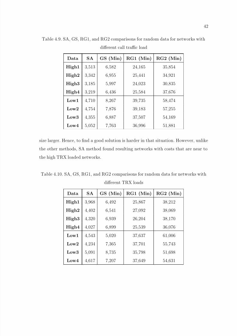
8/6/2019 Location Area Paging
http://slidepdf.com/reader/full/location-area-paging 53/65
42
Table 4.9. SA, GS, RG1, and RG2 comparisons for random data for networks with
different call traffic load
Data SA GS (Min) RG1 (Min) RG2 (Min)
High1 3,513 6,582 24,165 35,854
High2 3,342 6,955 25,441 34,921
High3 3,185 5,997 24,023 30,835
High4 3,219 6,436 25,584 37,676
Low1 4,710 8,267 39,735 58,474
Low2 4,754 7,876 39,183 57,255
Low3 4,355 6,887 37,507 54,169Low4 5,052 7,763 36,996 51,881
size larger. Hence, to find a good solution is harder in that situation. However, unlike
the other methods, SA method found resulting networks with costs that are near to
the high TRX loaded networks.
Table 4.10. SA, GS, RG1, and RG2 comparisons for random data for networks withdifferent TRX loads
Data SA GS (Min) RG1 (Min) RG2 (Min)
High1 3,968 6,492 25,867 38,212
High2 4,402 6,541 27,092 38,069
High3 4,320 6,939 26,204 38,170
High4 4,027 6,899 25,539 36,076
Low1 4,543 5,020 37,637 61,006
Low2 4,234 7,365 37,701 55,743
Low3 5,091 8,735 35,798 51,698
Low4 4,617 7,207 37,649 54,631

8/6/2019 Location Area Paging
http://slidepdf.com/reader/full/location-area-paging 54/65
43
5. CONCLUSIONS
The most important gain of the optimized LA planning is preventing needless
radio resource usage, which may be otherwise used for the communication of the cus-
tomers. Another gain is to be able to utilize the network elements more efficiently, and
therefore to decrease the number of network elements needed and reduce the network
construction costs.
In order to design a feasible cellular network, constraints related with the call
handling capacities of network elements and costs related with the paging and regis-
tration activities should be considered. Using the available network information in a
realistic manner, we formulated an optimization problem for the location area planning
and the assignment of cells to switches. We also proposed a solution technique based
on SA and a heuristic algorithm to the resulting difficult optimization problem. We
described the implementation details of the algorithm and compared it with some other
solution techniques.
For the comparison between SA and the other techniques three types of experi-
ments are performed. To guarantee the correctness, comparisons are done by running
the algorithms multiple times and taking the average or the minimum values of the
results. Real GSM network data (loads of the functional cells, etc.) is used in the first
type of experiments. It is found that SA based algorithm gives the best results com-
pared to other methods. Second best method was GS, however, the improvement of
the SA results compared to GS was approximately 50 per cent. For the second group of
experiments, to assure that the success of the SA based algorithm is not dependent to
a certain data set, randomly generated network data is used in the experiments. Again
SA performed best; however, in that group of experiments, the difference between SA
and the GS results were approximately 15 per cent.
The proposed heuristics algorithm (HOLAP) is also compared with SA and the
other methods in that experiment group. Neverthless, results found by HOLAP were

8/6/2019 Location Area Paging
http://slidepdf.com/reader/full/location-area-paging 55/65
44
poorer than SA and GS. The reason assumed for those worse results is described. The
last group of experiments is performed to investigate the methods on the networks with
different load characteristics. Again, the network data (the loads, etc.) was generatedrandomly. Though, for all kind of networks, SA gave better results compared to other
methods. Comments about the changes of SA performance for different network types
are given.
As a future work, a better heuristic algorithm could be developed that will be
aimed to solve our optimization problem. Beside that, our SA algorithm could also be
run on a wider test set to check the optimality of currently proposed SA parametervalues. Another extension to the problem stated in this work is to divide the problem
into two sub-problems. Firstly, assignment of cell to switches will be achieved, and
then assignment of LAs to BSs will be done. Hence, there will be two simpler objective
functions and the constraints stated in this work will be seperated to two sub-problems.
In summary, we believe that we have formulated a very general case of the LA
planning and cell assignment problem that includes the majority of the previously
proposed problems as its special cases. We have also proposed a promising algorithm
for the solution of this difficult optimization problem.

8/6/2019 Location Area Paging
http://slidepdf.com/reader/full/location-area-paging 56/65
45
APPENDIX A: PSEUDO-CODE OF SIMULATED
ANNEALING ALGORITHM
Simulated annealing algorithm consists of two main procedures. In the first part,
the initialization of the simulated annealing environment is done. The initial feasible
solution and the initial temperature is set. The pseudo-code of the first part can be
seen in Figure A.1.
P 0 = 0.999
α = 0.9999
choose the initial feasible network currentNw at random.
for InitialRunNumberLength( IN ) times do
begin
create a neighbor of currentNw and call it neighborNw.
if neighborNw is feasible then
begin
add the absolute value of cost difference
(cost of currentNw - cost of neighborNw) to TotalCost
set neighborNw as currentNw
end
end
∆E = TotalCost / InitialRunNumberLength
T = −∆E / ln (1/P 0)
Figure A.1. Initialization part
In the second part, annealing procedure is performed. The system searchs the
solution space for feasible solution till the one of the stopping criteria is reached. Thetemperature decrements and navigation in the solution space is controlled by the an-

8/6/2019 Location Area Paging
http://slidepdf.com/reader/full/location-area-paging 57/65
46
nealing procedure. The pseudo-code of the first part can be seen in Figure A.2.
bestNw = currentNw
repeat
n = 0
repeat
n = n + 1
create a neighbor of currentNw and call it neighborNw
if neighborNw is feasible then
if the cost of neighborNw (C n) is
lower than the cost of currentNw(C c) then
begin
currentNw = neighborNw
bestNw = currentNw
end
else
if e−(C n−C c)/T > random[0, 1) then
currentNw = neighborNw
until number of accepted neighbors is AD
or n is equal to number of BSs ∗ BSCs ∗ MSCs
update T = T * α
until cost is same for last WI temperature decrements
or maximum number of iterations (IL) is reached
Figure A.2. Annealing part

8/6/2019 Location Area Paging
http://slidepdf.com/reader/full/location-area-paging 58/65
47
REFERENCES
1. Saraydar, C. U., O. Kelly and C. Rose, “One-dimensional Location Area Design”,
IEEE Trans. on Vehicular Technology , Vol. 49, No. 5, pp. 1626-1633, September
2000.
2. Saraydar, C. U. and C. Rose, “Location Area Design Using Population and Traffic
Data”, Proc. of the CISS 1998 , Princeton, NJ, March 18-20, 1998.
3. Scourias, J., Overview of the Global System for Mobile Communications, 1997
http://ccnga.uwaterloo.ca/ jscouria/GSM/gsmreport.html.
4. Heine, G., GSM Networks: Protocols, Terminology, and Implementation , Artech
House Publishers, Boston, 1998.
5. Dong-Jun, L. and C. Dong-Ho, “On Optimum Timer Value of Area and Timer-
based Location Registration Scheme”, IEEE Communications Letters, Vol. 5, No.4, pp. 148-150, April 2001.
6. Ryu, S. H., K. H. Lee, Y. Y. Oh, J. Y. Lee and S. B. Lee, “Adaptive Time-Based
Location Update Scheme Using Fuzzy Logic”, IEEE International Conference on
Consumer Electronics, ICCE 1999 , pp. 322-323, Los Angeles, CA, June 20-24,
1999.
7. Fang, Y., I. Chlamtac and F. Hong-Ring, “Analytical Results for Optimal Choice
of Location Update Interval for Mobility Database Failure Restoration in PCS
Networks”, IEEE Transactions on Parallel and Distributed Systems, Vol. 11, No.
6, pp. 615-624, June 2000.
8. Mao, Z. and C. Douligeris, “Two Location Tracking Strategies for PCS Systems”,
Proceedings of Eight International Conference on Computer Communications and
Networks, IEEEE ICCCN 99 , Boston, pp. 318-323, October 11-13, 1999.

8/6/2019 Location Area Paging
http://slidepdf.com/reader/full/location-area-paging 59/65
48
9. Fang, Y., “Tradeoff Analysis for Location Update and Paging in Wireless Net-
works”, Proceedings of Global Telecommunications Conference(GLOBECOM),
2001, pp. 1754-1758, San Antonio, Texas, USA, November 25-29, 2001.
10. Casares-Giner, V. and J. Mataix-Oltra, “On Movement-Based Mobility Tracking
Strategy - An Enhanced Version”, IEEE Communications Letters, Vol. 2, No. 2,
pp. 45-47, Feb. 1998.
11. Tsai, J.-T. and H.-H. Hsiao, “Performance of Movement-based Location Update
and One-step Paging in Wireless Networks with Sparsely Underlaid Microcells”,
IEEE Global Telecommunications Conference(GLOBECOM ’01), Vol. 1, pp. 642
-647, 2001.
12. Jie, L., H. Kameda and K. Li, “Optimal Dynamic Mobility Management for PCS
Networks”, IEEE/ACM Transactions on Networking , Vol. 8, No. 3, pp. 319 -327,
June 2000.
13. Akyıldız, I. F., J. S. M. Ho and Y.-B. Lin, “Movement-based Location Update andSelective Paging for PCS Networks”, IEEE/ACM Transactions on Networking ,
Vol. 4, No. 4, pp. 629-638, Aug. 1996.
14. Akyıldız, I. F. and J.S.M. Ho, “A Mobile User Location Update and Paging Mech-
anism Under Delay Constraints”, Proceedings of ACM SIGCOMM’95 , Cambridge,
Massachusetts, USA, pp. 244-255, August 28 - September 1, 1995.
15. Wang, W. and I. F. Akyıldız, “Intersystem Location Update and Paging
Schemes for Multitier Wireless Networks”, Proc. ACM MobiCom’00 , Boston, Mas-
sachusetts, USA, August 6-11, 2000.
16. Wong, V. and V. Leung, “An Adaptive Distance-Based Location Update Algo-
rithm for Next-Generation PCS Networks”, IEEE Journal On Selected Areas In
Communications, Vol. 19, No. 10, pp. 1942-1952, October 2001.

8/6/2019 Location Area Paging
http://slidepdf.com/reader/full/location-area-paging 60/65
49
17. Abutaleb, A. and V. O. K. Li, “Location Update Optimization in Personal Com-
munication Systems”, ACM-Baltzer Journal of Wireless Networks (WINET), Vol.
3, No. 3, pp. 205-216, August 1997.
18. Verkama, M., “A Simple Implementation of Distance-Based Location Up-
dates”, IEEE 6th International Conference on Universal Personal Communica-
tions, ICVPC’97 , pp. 163-167, vol. 1, San Diego, CA, October, 12-16, 1997.
19. Zhang, J., “A Cell ID Assignment Scheme and Its Applications”, 29th International
Workshops on Parallel Processing, ICPP 2000 Workshop, pp. 507-512, Toronto,
Canada, August 21-24, 2000.
20. Wong, V. W.-S. and V. C. M. Leung, “An Adaptive Distance-based Location
Update Algorithm for PCS Networks”, IEEE International Conference on Com-
munications(ICC 2001), Vol. 7, pp. 2000-2005, Helsinki, Finland, June 11-14, 2001.
21. Bar-Noy, A., I. Kessler and M. Sidi, “Mobile Users: To Update or Not to Update?”,
Wireless Networks, Vol. 1, No. 2, pp. 175-185, July 1995.
22. Tabbane, S., “An Alternative Strategy for Location Tracking”, IEEE JSAC , Vol.
13, No. 5, pp. 880-892, June 1995.
23. Rose, C., “State-Based Paging/Registration: A Greedy Technique”, IEEE Trans-
actions on Vehicular Technology , Vol. 48, No. 1, pp. 166-173, January 1999.
24. Lei, Z., C. Saraydar and N. B. Mandayam, “Paging Area Optimization by Inter-
val Estimation for Wireless Personal Communication Networks” Mobile Networks
and Applications, 5 (2000), 1, Special Issue on Mobile Data Networks: Advanced
Technologies and Services, pp. 85-99, 2000.
25. Pollini, G. P. and I. Chin Lin, “A Profile-Based Location Strategy and Its Perfor-
mance”, IEEE Journal on Selected Areas in Communications, Vol. 15, No. 8, pp.
1415-1424, October 1997.

8/6/2019 Location Area Paging
http://slidepdf.com/reader/full/location-area-paging 61/65
50
26. DasBit, S. and S. Mitra, “A Varying Per User Profile Based Location Update Strat-
egy for Cellular Networks”, IFIP/IEEE 7th International Conference on Com-
munication Technology(WCC - ICCT 2000), Vol. 1, pp. 754-760, Beijing, China,August 21-23, 2000.
27. Adly, N. and A. El-Nahas, “A Profile-based Hierarchical Location Management
Scheme for Future PCS”, 11th International Workshop on Database and Expert
Systems Applications, pp. 204-208, Greenwich, London, UK, September 6-8, 2000.
28. Wang, K., J.-M. Liao and J.-M. Chen, “Intelligent Location Tracking Strategy in
PCS”, IEE Proceedings - Communications, Vol. 147, No. 1, pp. 63-68, Feb. 2000.
29. Subrata, R. and A.Y. Zomaya, “Location Management in Mobile Computing”,
Proceedings of ACS/IEEE Int. Conf. on Computer Systems and Applications, 2001,
pp. 287-289, Beirut, Lebanon, June 26-29, 2001.
30. Pitoura, E. and G. Samaras, “Locating Objects in Mobile Computing”, IEEE
Transactions on Knowledge and Data Engineering , Vol. 13, No. 4, pp. 571-592,July-Aug, 2001.
31. Liu, H.-I. and C.-P. Liu, “A Geography Based Location Management Scheme
for Wireless Personal Communication Systems”, IEEE 51st Vehicular Technology
Conference(VTC 2000), Vol. 2, pp. 1358-1361, Spring, Tokyo, 2000.
32. Zhou, S., A. Seneviratne and T. Percival, “A Location Management Scheme for
Mobility Support in Wireless IP Networks Using Session Initiation Protocol (SIP)”,
Ninth IEEE International Conference on Networks, pp. 486-491, Bangkok, Thai-
land, October 10-12, 2001.
33. Kin, W. N. and V. C. M. Leung, “An IPv6-based Location Management Scheme for
Client-Server Computing Over Mobile Data Networks”, IEEE Wireless Commu-
nications and Networking Conference(WCNC 1999), Vol. 1, pp. 525 -529, Antibes,
France, July 4-7, 1999.
8/6/2019 Location Area Paging
http://slidepdf.com/reader/full/location-area-paging 62/65
51
34. Kim, D.-H., B.-D. Park and Y.-Z. Cho, “Adaptive Location Management Scheme
for PNNI-based Hierarchical Wireless ATM Networks”, IEEE Region 10 Interna-
tional Conference on Electrical and Electronic Technology(TENCON 2001), Vol.2,pp. 571-574, Phuket Island - Langkawi Island, August 19-22, 2001.
35. Kim, D.H., S. C. Song, J. Y. Lee, W. Z. Cui, W. K. Choi and S. S. An, “Dynamic
Location Management Scheme for Location Registers in Wireless ATM Networks”,
IEEE Electronics Letters, Vol. 36, No. 19, pp. 1650-1651, Sept. 2000.
36. McNair, J., “Location Registration and Paging in Mobile Satellite Systems”, Fifth
IEEE Symposium on Computers and Communications(ISCC 2000), pp. 232-237,
2000.
37. Ratnam, K., I. Matta and S. Rangarajan, “A Fully Distributed Location Manage-
ment Scheme for Large PCS”, Fifth IEEE Symposium on Computers and Com-
munications(ISCC 2000), pp. 514-519, 2000.
38. Zuji, M. and C. Douligeris, “High Throughput Database Structures for LocationManagement in PCS Networks”, 19th Annual Joint Conference of the IEEE Com-
puter and Communications Societies(INFOCOM 2000), Vol. 2, pp. 785-794, Tel
Aviv, Israel, March 26-30, 2000.
39. Shankaran, R., V. Varadharajan and M. Hitchens, “A Distributed Location Man-
agement Scheme for Mobile Hosts”, Eighth International Conference on Parallel
and Distributed Systems(ICPADS 2001), pp. 297-304, KyongJu City, Korea, June
26-29, 2001.
40. Minh, H. N. and H. R. van As, “Performance Analysis of Distributed Location
Management for Wireless Networks 15th International Conference on Information
Networking , pp. 25-31, Beppu City, Japan, January 31 - February 2, 2001.
41. Chiang, K.-H. and N. Shenoy, “A Random Walk Mobility Model for Location
Management in Wireless Networks”, 12th IEEE International Symposium on Per-

8/6/2019 Location Area Paging
http://slidepdf.com/reader/full/location-area-paging 63/65
52
sonal, Indoor and Mobile Radio Communications, PIMRC 2001, Vol. 2, pp. 43-48,
San Diego, CA, September 30 - October 3, 2001.
42. Scourias, J. and T. Kunz, “Activity-based Mobility Modeling: Realistic Evaluation
of Location Management Schemes for Cellular Networks”, Proceedings of IEEE
Wireless Communications and Networking Conference(WCNC 1999), pp. 296-300,
New Orleans, LA, September 21-24, 1999.
43. Akyıldız, I. F., Y.-B. Lin, W.-R. Lai and R.-J. Chen, “A New Random Walk Model
for PCS Networks”, IEEE Journal on Selected Areas in Communications, Vol. 18,
No. 7, pp. 1254-1260, July 2000.
44. Yang, M. H., L.-W. Chen, Y.-C. Tseng and J.-P. Sheu, “A Traveling Salesman
Mobility Model and Its Location Tracking in PCS Networks”, 21st International
Conference on Distributed Computing Systems, ICDS’01, pp. 517-523, Phoenix,
Arizona, April 16-19, 2001.
45. Tonguz, O. K., S. Mishra and R. Josyula, “Intelligent Paging in Wireless Networks:Random Mobility Models and Grouping Algorithms for Locating Subscribers”,
Proc. of IEEE 49th Vehicular Technology Conference, Vol. 2, pp. 1177-1181, Hous-
ton, Texas, May 16-20, 1999.
46. Metropolis, N., A. W. Rosenbluth, M. N. Rosenbluth, A. H. Teller and E. Teller,
“Equation of State Calculations by Fast Computing Machines”, Journal of Chem-
ical Physics, Vol. 21, No. 6, pp. 1087-1092, June 1953.
47. Kirkpatrick, S., C. D. Gelatt and M. P. Vecchi, “Optimization by Simulated
Annealing”, Science, Vol. 220, pp. 671-680, May 1983.
48. Johnson, D. S., C. R. Aragon, L. A. McGeoch and C. Schevon, “Optimization by
Simulated Annealing: An Experimental Evaluation; Part1, Graph Partitioning”,
Operation Research , Vol. 37, No. 6, pp. 865-892, November-December 1989.

8/6/2019 Location Area Paging
http://slidepdf.com/reader/full/location-area-paging 64/65
53
49. Aarts, E. H., J. Korst and P. J. van Laarhoven, Simulated Annealing , In E.
Aarts and Lenstra J. K. (editors), Local Search in Combinatorial Optimization,
pp. 91-120, John Wiley & Sons Ltd., Chichester, 1997.
50. Chen, H., N. S. Flann and D. W. Watson, “Parallel Genetic Simulated Anneal-
ing: A Massively Parallel SIMD Approach”, IEEE Transactions on Parallel and
Distributed Computing , Vol. 9, No. 2, pp. 126-136, Feb. 1998.
51. Yip, P. P. C. and Y. H. Pao, “Combinatorial Optimization with Use of Guided
Evolutionary Simulated Annealing”, IEEE Transactions on Neural Networks, Vol.
6, No. 2, pp. 290-295, March 1995.
52. Herault, L., “Rescaled simulated annealing” In World Congress of Computational
Intelligence, IJCNN’98, Proceedings, pp. 1239-1244, Anchorage, Alaska, May 4-9,
1998.
53. Barral, D., J. P. Perrin, E. Dombre and A. Liegeois “An Evolutionary Simulated
Annealing Algorithm for Optimizing Robotic Task Point Ordering” Proceedingsof the 1999 IEEE International Symposium on Assembly and Task Planning , pp.
157-162, Porto (Portugal), 21-24 July 1999.
54. Rich, E. and R. Knight, Artificial Intelligence, McGraw-Hill, New York, 1991.
55. Hajek, B., “Cooling Schedules for Optimal Annealing”, Mathematics of Operations
Research , Vol. 13, No. 2, pp. 311-329, May 1988.
56. Demirkol, I., C. Ersoy, M. U. Caglayan and H. Delic, “Location Area Planning in
Cellular Networks Using Simulated Annealing”, Proceedings of IEEE Infocom, The
Conference on Computer Communications 2001, pp. 13-20, Anchorage, Alaska,
April 22-26, 2001.
57. Bogazici University Computer Engineering Department, BU ASMA Project Home
Page, 1999 http://www.asma.cmpe.boun.edu.tr.

8/6/2019 Location Area Paging
http://slidepdf.com/reader/full/location-area-paging 65/65
54
58. Elmohamed, S., P. Coddington and G. Fox, “A Comparison of Annealing Tech-
niques for Academic Course Scheduling”, Proceedings of the 2nd International
Conference on the Practice and Theory of Automated Timetabling PATAT ’97 , pp146-166, University of Toronto, Canada, August 20-22, 1997.
59. Hart, W. E., “A Theoretical Comparison of Evolutionary Algorithms and Sim-
ulated Annealing”, Proc. of 5th Annual Conf. on Evolutionary Programming
(EP96), pp. 147-154, San Diego, CA, February 29 - March 3, 1996.


![AP-SPS180 SIP Paging Server PT [호환 모드] AP-SPS180 SIP Paging Server • Signaling Server – SIP Application Server, Proxy, Registrar and Location Server (RFC3261) – Multiple](https://img.pdfslide.us/doc/110x75/601be417fc011a5c6b76c626/ap-sps180-sip-paging-server-pt-eeoe-ap-sps180-sip-paging-server-a-signaling.jpg)