Embed Size (px)
Citation preview

Locating Sensors in Complex Chemical Plants Basedon Fault Diagnostic Observability Criteria
Rao Raghuraj, Mani Bhushan, and Raghunathan RengaswamyDept. of Chemical Engineering, Indian Institute of Technology, Bombay Powai, Mumbai-400 076, India
Fault diagnosis is an important task for the safe and optimal operation of chemicalprocesses. Hence, this area has attracted considerable attention from researchers in thepast few years. A ®ariety of approaches ha®e been proposed for sol®ing this problem. Allapproaches for fault detection and diagnosis in some sense in®ol®e the comparison ofthe obser®ed beha®ior of the process to a reference model. The process beha®ior isinferred using sensors measuring the important ®ariables in the process. Hence, theefficiency of the diagnostic approach depends critically on the location of sensors moni-toring the process ®ariables. The emphasis of most of the work on fault diagnosis hasbeen more on procedures to perform diagnosis gi®en a set of sensors and less on theactual location of sensors for efficient identification of faults. A digraph-based approachis proposed for the problem of sensor location for identification of faults. Various graphalgorithms that use the de®eloped digraph in deciding the location of sensors based onthe concepts of obser®ability and resolution are discussed. Simple examples are pro®idedto explain the algorithms, and a complex FCCU case study is also discussed to under-score the utility of the algorithm for large flow sheets. The significance and scope of theproposed algorithms are highlighted.
Introduction
The process disturbances or faults, if undetected, have aserious impact on process economy, product quality, safety,productivity, and pollution level. In order to detect, diagnose,and correct these abnormal process behaviors, efficient andadvanced automated diagnostic systems are of great impor-tance to modern complex chemical industries. Considerableresearch has gone into the development of such diagnosticsystems. Expert systems, neural networks, rule-based tech-niques, and signed directed graphs are some of the diagnosticapproaches discussed in the literature.
These techniques basically involve the following steps.1. Fault detection: Observing the fault symptoms in mea-
sured values and detecting that a fault has occurred.2. Fault identification:
Ž .a Classification: Determining the type of the fault.Ž .b Estimation: Determining the extent of the fault.Ž .c Diagnosis: Determining the root cause of the fault.
Correspondence concerning this article should be addressed to R. Rengaswamy.
3. Correction: Correcting the system by repairing or replac-ing.
Whenever a process encounters a fault, the effect of thisfault is propagated to all or some of the process variables.The main objective of the fault-diagnosis step is to observethese fault symptoms and determine the root cause for theobserved behavior. The fault-detection step involves compar-ing the observed behavior of the process to a reference model.This observed fault-symptom pattern forms the basis for thefault-identification step. Thus the efficiency of the diagnosticsystem depends critically upon the location of the sensorsmonitoring important process variables. With hundreds ofprocess variables available for measurement in any chemicalplant, selection of crucial and optimum sensor positions posesa unique problem. Hence there is a need for an automatedprocedure to design a cost-optimum, foolproof, and highlyreliable fault-monitoring system for the safe operation of atypical industrial process.
Knowledge of fault propagation within the system is neces-sary for developing a solution to the preceding problem. Dif-
February 1999 Vol. 45, No. 2 AIChE Journal310
ferent approaches, such as fault trees and digraphs, are avail-able in the literature to obtain fault propagation behavior inthe presence of a fault. A fault tree is a logic tree that propa-gates primary events or faults to a top-level event or a haz-ard. Hence, such a tree would give the propagation of theeffect of a fault to various process variables. Signed digraphŽ .SDG is another technique that is concerned with the
Ž . Žcause]effect CE analysis of the system Iri et al., 1979;. Ž .O’Shima et al., 1985 . Iri et al. 1979 were the first to intro-
duce an algorithm for such a CE diagnosis of system failures,Ž .based on signed directed graphs SDG . Kramer and Palow-
Ž .itch 1987 developed a rule-based approach for identifyingthe possible causes of process disturbances using the SDG
Ž .representation. Chang and Yu 1990 also gave a systematicdesign procedure for constructing the rule-based fault-di-agnostic system using the SDG. They simplified the SDG ac-cording to states, so as to overcome problems associated withspurious and erroneous interpretations in the SDG. Mohin-
Ž .dra and Clark 1993 used the SDG to come up with a dis-tributed fault-diagnosis methodology.
Some work has already been done on using these tech-Ž .niques to locate sensors. Lambert 1977 used fault-trees to
analyze the location of sensors depending on the effect ofŽ .basic units fault origins on the process variables. Even
though this work was the first step toward the design of sen-sor locations based on a diagnostic observability criterion, it
Ž . Ž .had drawbacks such as: 1 inability to handle cycles, and 2the development of a fault tree is in itself an error-prone andtime-consuming process. A quantitative approach for sensornetwork design based on failure probabilities was also ex-
Ž .plained by Lambert 1977 . To solve the problem of observ-ability, based on the process graph, Ali and Narasimhan have
Žpresented sensor network design strategies for linear Ali and. ŽNarasimhan, 1993, 1995 and bilinear Ali and Narasimhan,
.1996 processes. They dealt with multicomponent mass flowprocesses and energy distribution networks. Using the con-cepts of fault observability and fault resolution, Chang et al.Ž .1993 developed a new optimal design strategy for fault-monitoring systems. A trial-and-error algorithm was pro-posed that utilizes the concept of a diagnostic efficiency table.The ability to utilize quantitative failure probability data wasnot incorporated in their approach. There are also othermethods based on linear and bilinear mathematical models
Ž .for sensor location Madron and Veverka, 1992 . Thesemethods are not reviewed here because the solution strategyproposed in this article is fundamentally different. We ap-proach the sensor-location problem through a qualitative CEanalysis of various fault scenarios.
The importance of the problem of sensor location is evi-dent, as all the fault-diagnosis techniques depend on a givenset of observed fault symptoms. The emphasis of most of thework on fault diagnosis has been more on procedures to per-form diagnosis given a set of sensors and less on the actuallocation of sensors for efficient identification of faults. In thisarticle, a digraph-based approach is proposed for the prob-lem of sensor location for the identification of faults. Thedigraph-based approach has many advantages. It involves asimple graphical representation of the process that is easy toanalyze. A few researchers have already looked at the prob-lem of automatic development of digraphs from the process
Ž .model equations Iri et al., 1979; Mylaraswamy et al., 1994 .
The qualitative SDG model is sufficient to observe the ef-fects of faults on different process variables, avoiding com-plex mathematical relationships between various processvariables.
In our solution to the problem of sensor location, digraphsare used to infer the propagation behavior when differentfaults occur. The sensor location problem is posed at two lev-els. First, the problem of identifying a minimum number ofsensor locations for observing all the faults is formulated andsolved. Second, the problem of maximum resolution of faultsunder single-fault and multiple-fault assumptions is formu-lated. It is shown that the same algorithm proposed for theobservability problem can be used in solving these problemsalso.
Qualitative Analysis of Sensor LocationSigned-directed-graph approach
The ultimate aim of this work is the design of efficientmonitoring systems that will help in quick and efficient iden-
Ž .tification of faults. The directed graph DG that representsthe CE behavior of the process is used as a basis for thesensor-location algorithm. Most of the work done on faultdiagnosis uses the SDG representing the process. The onlydifference between DG and SDG is that signs are placed onthe arcs of DG to get an SDG. However, the structure of theDG and SDG are exactly the same. Hence, in this section wewill briefly review the work done on using SDG in processfault diagnosis to emphasize the importance of proper sensorlocation for efficient fault diagnosis. SDG is a graphical rep-resentation of the system that utilizes nodes and branches.The nodes correspond to the process state variables and mal-functions, and the branches represent the causal relation-ships between the process variables. A given system can berepresented structurally in the form of an SDG. All possiblevariables and parameters of the system are clearly definedand are represented as nodes. The model equations areproperly arranged, and the effects of a particular variable onother nodes are obtained. The branch sign is fixed accordingto the relationship between the variables represented as itsend nodes. The positive and negative influences are shown byassigning q and y signs, respectively, to the branches. Thestates of the variables are represented by assigning nodes q,0, or ysigns for high, normal, and low states, respectively.This representation helps in defining a pattern of observedsymptoms on the process SDG. A nonzero node sign signifiesthe presence of a failure in the process, and a set of nonzerosigns in the SDG represents a pattern of fault symptoms. It iswell understood that all the variables of the process in a com-plex chemical plant cannot be measured due to technical andeconomical infeasibilities. The pattern defined is thereforealways partially observed and is hence called ‘‘the partial pat-tern.’’
This partial pattern can be used to obtain the CE graph tofind the structure of fault propagation. The CE graph con-
Žsists of so-called strongly connected components Iri et al.,.1979 . To aid the fault-diagnosis studies, a node or a cycle
with no input arcs is considered to be a maximally stronglyŽ .connected component MSCC in the SDG. A branch is said
to be consistent if its sign is equal to the product of both ofthe node signs it is connected with. And a nonzero node is
February 1999 Vol. 45, No. 2AIChE Journal 311
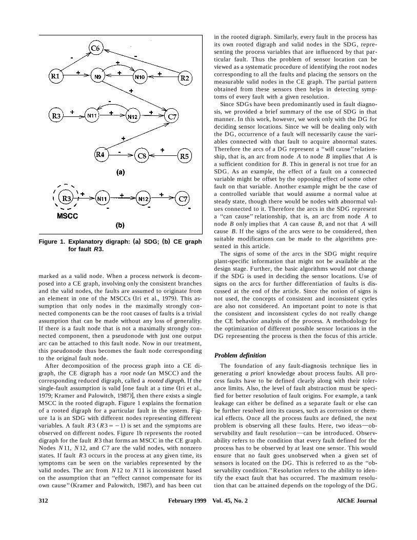
( ) ( )Figure 1. Explanatory digraph: a SDG; b CE graphfor fault R3.
marked as a valid node. When a process network is decom-posed into a CE graph, involving only the consistent branchesand the valid nodes, the faults are assumed to originate from
Ž .an element in one of the MSCCs Iri et al., 1979 . This as-sumption that only nodes in the maximally strongly con-nected components can be the root causes of faults is a trivialassumption that can be made without any loss of generality.If there is a fault node that is not a maximally strongly con-nected component, then a pseudonode with just one outputarc can be attached to this fault node. Now in our treatment,this pseudonode thus becomes the fault node correspondingto the original fault node.
After decomposition of the process graph into a CE di-Ž .graph, the CE digraph has a root node an MSCC and the
corresponding reduced digraph, called a rooted digraph. If thew Žsingle-fault assumption is valid one fault at a time Iri et al.,
.x1979; Kramer and Palowitch, 1987 , then there exists a singleMSCC in the rooted digraph. Figure 1 explains the formationof a rooted digraph for a particular fault in the system. Fig-ure 1a is an SDG with different nodes representing different
Ž .variables. A fault R3 R3sy1 is set and the symptoms areobserved on different nodes. Figure 1b represents the rooteddigraph for the fault R3 that forms an MSCC in the CE graph.Nodes N11, N12, and C7 are the valid nodes, with nonzerostates. If fault R3 occurs in the process at any given time, itssymptoms can be seen on the variables represented by thevalid nodes. The arc from N12 to N11 is inconsistent basedon the assumption that an ‘‘effect cannot compensate for its
Ž .own cause’’ Kramer and Palowitch, 1987 , and has been cut
in the rooted digraph. Similarly, every fault in the process hasits own rooted digraph and valid nodes in the SDG, repre-senting the process variables that are influenced by that par-ticular fault. Thus the problem of sensor location can beviewed as a systematic procedure of identifying the root nodescorresponding to all the faults and placing the sensors on themeasurable valid nodes in the CE graph. The partial patternobtained from these sensors then helps in detecting symp-toms of every fault with a given resolution.
Since SDGs have been predominantly used in fault diagno-sis, we provided a brief summary of the use of SDG in thatmanner. In this work, however, we work only with the DG fordeciding sensor locations. Since we will be dealing only withthe DG, occurrence of a fault will necessarily cause the vari-ables connected with that fault to acquire abnormal states.Therefore the arcs of a DG represent a ‘‘will cause’’ relation-ship, that is, an arc from node A to node B implies that A isa sufficient condition for B. This in general is not true for anSDG. As an example, the effect of a fault on a connectedvariable might be offset by the opposing effect of some otherfault on that variable. Another example might be the case ofa controlled variable that would assume a normal value atsteady state, though there would be nodes with abnormal val-ues connected to it. Therefore the arcs in the SDG representa ‘‘can cause’’ relationship, that is, an arc from node A tonode B only implies that A can cause B, and not that A willcause B. If the signs of the arcs were to be considered, thensuitable modifications can be made to the algorithms pre-sented in this article.
The signs of some of the arcs in the SDG might requireplant-specific information that might not be available at thedesign stage. Further, the basic algorithms would not changeif the SDG is used in deciding the sensor locations. Use ofsigns on the arcs for further differentiation of faults is dis-cussed at the end of the article. Since the notion of signs isnot used, the concepts of consistent and inconsistent cyclesare also not considered. An important point to note is thatthe consistent and inconsistent cycles do not really changethe CE behavior analysis of the process. A methodology forthe optimization of different possible sensor locations in theDG representing the process is then the focus of this article.
Problem definitionThe foundation of any fault-diagnosis technique lies in
generating a priori knowledge about process faults. All pro-cess faults have to be defined clearly along with their toler-ance limits. Also, the level of fault abstraction must be speci-fied for better resolution of fault origins. For example, a tankleakage can either be defined as a separate fault or else canbe further resolved into its causes, such as corrosion or chem-ical effects. Once all the process faults are defined, the nextproblem is observing all these faults. Here, two ideas}ob-servability and fault resolution}can be introduced. Observ-ability refers to the condition that every fault defined for theprocess has to be observed by at least one sensor. This wouldensure that no fault goes unobserved when a given set ofsensors is located on the DG. This is referred to as the ‘‘ob-servability condition.’’ Resolution refers to the ability to iden-tify the exact fault that has occurred. The maximum resolu-tion that can be attained depends on the topology of the DG.
February 1999 Vol. 45, No. 2 AIChE Journal312
Hence, given the constraints on measurement points, theproblem of resolution is generating sensor locations so thatevery fault is resolved to the maximum extent possible. Thiscondition is referred to as the ‘‘highest fault resolution.’’
As we have seen, for a fault in the system, there exists arooted digraph and a corresponding root node. This rooteddigraph involves all the consistent branches through whichthe fault propagates before terminating at some node ornodes. Hence for a particular number of process faults, thereare an equal number of possible rooted digraphs in the DG.Since a rooted digraph passes through various valid nodes,there is the possibility that different rooted digraphs havesome common valid nodes. It is obvious that in a connectedgraph, some, if not all, of the rooted digraphs have commonvalid nodes through which they pass independently. Thismeans that two or more faults can affect the same variable inthe process. Hence, by keeping a sensor on such a node thefault symptoms of all connected root nodes can be observed.
Definition of Key Component. The problem of sensor loca-tion in order to observe all the faults now reduces to that offinding a set of nodes that would have a directed path fromall the root nodes. For convenience, these nodes are referredto as the ‘‘key components.’’ For example, in Figure 1a nodesC7 and C8 would form a set of key components that wouldhave a directed path from every root node. Again, the set C6,C7, C8 would also form a set of key components. Hence, ofall the sets of key components, there could be a minimum setwith a minimum number of key components. This set wouldcontain the minimum number of sensors that would satisfythe observability condition. In the next section, we solve theproblem of finding a set of sensors that would observe all thefaults in any given process DG, and then the problem of find-ing a minimum set of sensors will be addressed.
Sensor Location and Fault Obser®ability
Problem 1: Sensor Location for Fault Obser®ability. Given aprocess DG, the sensor location problem for observability isone of finding a set of nodes that is connected to all the
Ž .nodes with only output arcs root nodes .The basic idea that is used in solving the problem is based
on the following claim.ŽClaim 1. In a DG that is weakly connected i.e., the cor-
.responding undirected graph is connected with no cycles,Žthere is at least one directed path from a root node node
.with only output arcs to one of the nodes with only inputarcs.
Proof of Claim 1. Consider a node with only output arcs.Consider the longest directed path from the node to someother node in the DG. Now, the last node in the directedpath should be a node with only input arcs, otherwise it wouldnot be the longest path. Hence every root node is connectedthrough a directed path to one of the nodes with only inputarcs. It is clear that Claim 1 is valid only for DG with nocycles.
Given a process DG, the observability problem is solvedthrough the following sequence of steps.
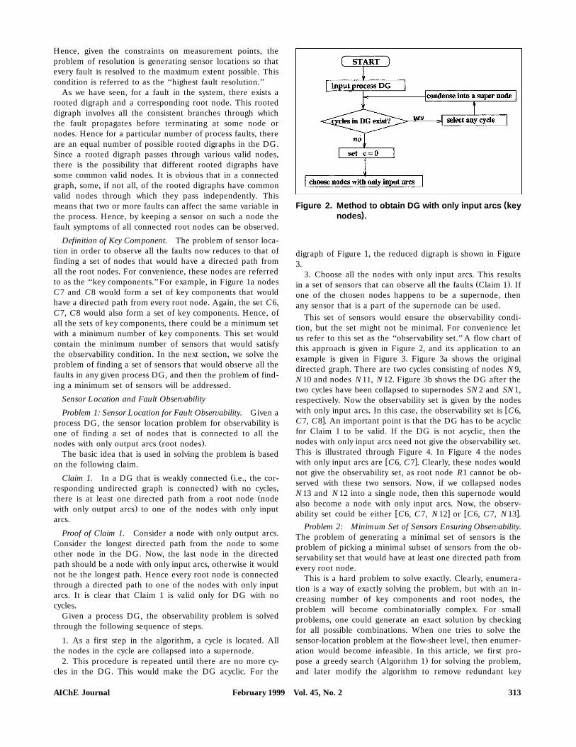
1. As a first step in the algorithm, a cycle is located. Allthe nodes in the cycle are collapsed into a supernode.
2. This procedure is repeated until there are no more cy-cles in the DG. This would make the DG acyclic. For the
(Figure 2. Method to obtain DG with only input arcs key)nodes .
digraph of Figure 1, the reduced digraph is shown in Figure3.
3. Choose all the nodes with only input arcs. This resultsŽ .in a set of sensors that can observe all the faults Claim 1 . If
one of the chosen nodes happens to be a supernode, thenany sensor that is a part of the supernode can be used.
This set of sensors would ensure the observability condi-tion, but the set might not be minimal. For convenience letus refer to this set as the ‘‘observability set.’’ A flow chart ofthis approach is given in Figure 2, and its application to anexample is given in Figure 3. Figure 3a shows the originaldirected graph. There are two cycles consisting of nodes N9,N10 and nodes N11, N12. Figure 3b shows the DG after thetwo cycles have been collapsed to supernodes SN2 and SN1,respectively. Now the observability set is given by the nodes
wwith only input arcs. In this case, the observability set is C6,xC7, C8 . An important point is that the DG has to be acyclic
for Claim 1 to be valid. If the DG is not acyclic, then thenodes with only input arcs need not give the observability set.This is illustrated through Figure 4. In Figure 4 the nodes
w xwith only input arcs are C6, C7 . Clearly, these nodes wouldnot give the observability set, as root node R1 cannot be ob-served with these two sensors. Now, if we collapsed nodesN13 and N12 into a single node, then this supernode wouldalso become a node with only input arcs. Now, the observ-
w x w xability set could be either C6, C7, N12 or C6, C7, N13 .Problem 2: Minimum Set of Sensors Ensuring Obser®ability.
The problem of generating a minimal set of sensors is theproblem of picking a minimal subset of sensors from the ob-servability set that would have at least one directed path fromevery root node.
This is a hard problem to solve exactly. Clearly, enumera-tion is a way of exactly solving the problem, but with an in-creasing number of key components and root nodes, theproblem will become combinatorially complex. For smallproblems, one could generate an exact solution by checkingfor all possible combinations. When one tries to solve thesensor-location problem at the flow-sheet level, then enumer-ation would become infeasible. In this article, we first pro-
Ž .pose a greedy search Algorithm 1 for solving the problem,and later modify the algorithm to remove redundant key
February 1999 Vol. 45, No. 2AIChE Journal 313
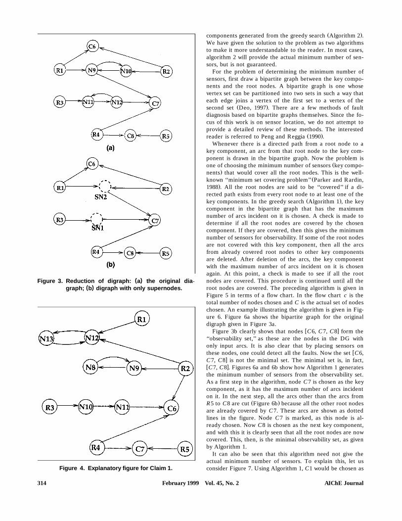
( )Figure 3. Reduction of digraph: a the original dia-( )graph; b digraph with only supernodes.
Figure 4. Explanatory figure for Claim 1.
Ž .components generated from the greedy search Algorithm 2 .We have given the solution to the problem as two algorithmsto make it more understandable to the reader. In most cases,algorithm 2 will provide the actual minimum number of sen-sors, but is not guaranteed.
For the problem of determining the minimum number ofsensors, first draw a bipartite graph between the key compo-nents and the root nodes. A bipartite graph is one whosevertex set can be partitioned into two sets in such a way thateach edge joins a vertex of the first set to a vertex of the
Ž .second set Deo, 1997 . There are a few methods of faultdiagnosis based on bipartite graphs themselves. Since the fo-cus of this work is on sensor location, we do not attempt toprovide a detailed review of these methods. The interested
Ž .reader is referred to Peng and Reggia 1990 .Whenever there is a directed path from a root node to a
key component, an arc from that root node to the key com-ponent is drawn in the bipartite graph. Now the problem is
Žone of choosing the minimum number of sensors key compo-.nents that would cover all the root nodes. This is the well-
Žknown ‘‘minimum set covering problem’’ Parker and Rardin,.1988 . All the root nodes are said to be ‘‘covered’’ if a di-
rected path exists from every root node to at least one of theŽ .key components. In the greedy search Algorithm 1 , the key
component in the bipartite graph that has the maximumnumber of arcs incident on it is chosen. A check is made todetermine if all the root nodes are covered by the chosencomponent. If they are covered, then this gives the minimumnumber of sensors for observability. If some of the root nodesare not covered with this key component, then all the arcsfrom already covered root nodes to other key componentsare deleted. After deletion of the arcs, the key componentwith the maximum number of arcs incident on it is chosenagain. At this point, a check is made to see if all the rootnodes are covered. This procedure is continued until all theroot nodes are covered. The preceding algorithm is given inFigure 5 in terms of a flow chart. In the flow chart c is thetotal number of nodes chosen and C is the actual set of nodeschosen. An example illustrating the algorithm is given in Fig-ure 6. Figure 6a shows the bipartite graph for the originaldigraph given in Figure 3a.
w xFigure 3b clearly shows that nodes C6, C7, C8 form the‘‘observability set,’’ as these are the nodes in the DG withonly input arcs. It is also clear that by placing sensors on
wthese nodes, one could detect all the faults. Now the set C6,xC7, C8 is not the minimal set. The minimal set is, in fact,
w xC7, C8 . Figures 6a and 6b show how Algorithm 1 generatesthe minimum number of sensors from the observability set.As a first step in the algorithm, node C7 is chosen as the keycomponent, as it has the maximum number of arcs incidenton it. In the next step, all the arcs other than the arcs from
Ž .R5 to C8 are cut Figure 6b because all the other root nodesare already covered by C7. These arcs are shown as dottedlines in the figure. Node C7 is marked, as this node is al-ready chosen. Now C8 is chosen as the next key component,and with this it is clearly seen that all the root nodes are nowcovered. This, then, is the minimal observability set, as givenby Algorithm 1.
It can also be seen that this algorithm need not give theactual minimum number of sensors. To explain this, let usconsider Figure 7. Using Algorithm 1, C1 would be chosen as
February 1999 Vol. 45, No. 2 AIChE Journal314
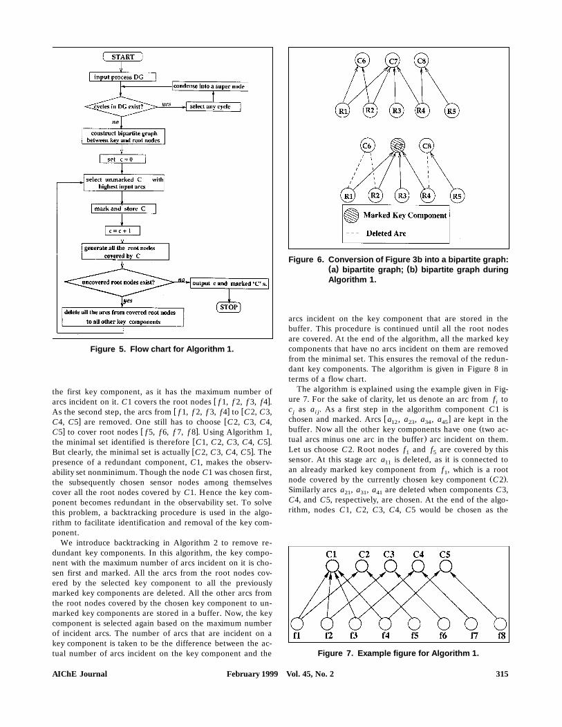
Figure 5. Flow chart for Algorithm 1.
the first key component, as it has the maximum number ofw xarcs incident on it. C1 covers the root nodes f 1, f 2, f 3, f4 .
w x wAs the second step, the arcs from f 1, f 2, f 3, f4 to C2, C3,x wC4, C5 are removed. One still has to choose C2, C3, C4,
x w xC5 to cover root nodes f5, f6, f 7, f 8 . Using Algorithm 1,w xthe minimal set identified is therefore C1, C2, C3, C4, C5 .w xBut clearly, the minimal set is actually C2, C3, C4, C5 . The
presence of a redundant component, C1, makes the observ-ability set nonminimum. Though the node C1 was chosen first,the subsequently chosen sensor nodes among themselvescover all the root nodes covered by C1. Hence the key com-ponent becomes redundant in the observability set. To solvethis problem, a backtracking procedure is used in the algo-rithm to facilitate identification and removal of the key com-ponent.
We introduce backtracking in Algorithm 2 to remove re-dundant key components. In this algorithm, the key compo-nent with the maximum number of arcs incident on it is cho-sen first and marked. All the arcs from the root nodes cov-ered by the selected key component to all the previouslymarked key components are deleted. All the other arcs fromthe root nodes covered by the chosen key component to un-marked key components are stored in a buffer. Now, the keycomponent is selected again based on the maximum numberof incident arcs. The number of arcs that are incident on akey component is taken to be the difference between the ac-tual number of arcs incident on the key component and the
Figure 6. Conversion of Figure 3b into a bipartite graph:( ) ( )a bipartite graph; b bipartite graph duringAlgorithm 1.
arcs incident on the key component that are stored in thebuffer. This procedure is continued until all the root nodesare covered. At the end of the algorithm, all the marked keycomponents that have no arcs incident on them are removedfrom the minimal set. This ensures the removal of the redun-dant key components. The algorithm is given in Figure 8 interms of a flow chart.
The algorithm is explained using the example given in Fig-ure 7. For the sake of clarity, let us denote an arc from f toic as a . As a first step in the algorithm component C1 isj i j
w xchosen and marked. Arcs a , a , a , a are kept in the12 23 34 45Žbuffer. Now all the other key components have one two ac-
.tual arcs minus one arc in the buffer arc incident on them.Let us choose C2. Root nodes f and f are covered by this1 5sensor. At this stage arc a is deleted, as it is connected to11an already marked key component from f , which is a root1
Ž .node covered by the currently chosen key component C2 .Similarly arcs a , a , a are deleted when components C3,21 31 41C4, and C5, respectively, are chosen. At the end of the algo-rithm, nodes C1, C2, C3, C4, C5 would be chosen as the
Figure 7. Example figure for Algorithm 1.
February 1999 Vol. 45, No. 2AIChE Journal 315
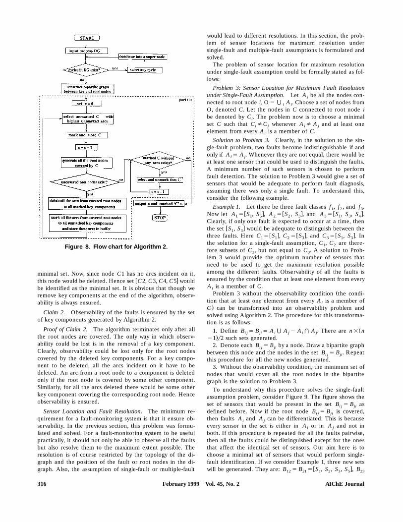
Figure 8. Flow chart for Algorithm 2.
minimal set. Now, since node C1 has no arcs incident on it,w xthis node would be deleted. Hence set C2, C3, C4, C5 would
be identified as the minimal set. It is obvious that though weremove key components at the end of the algorithm, observ-ability is always ensured.
Claim 2. Observability of the faults is ensured by the setof key components generated by Algorithm 2.
Proof of Claim 2. The algorithm terminates only after allthe root nodes are covered. The only way in which observ-ability could be lost is in the removal of a key component.Clearly, observability could be lost only for the root nodescovered by the deleted key components. For a key compo-nent to be deleted, all the arcs incident on it have to bedeleted. An arc from a root node to a component is deletedonly if the root node is covered by some other component.Similarly, for all the arcs deleted there would be some otherkey component covering the corresponding root node. Henceobservability is ensured.
Sensor Location and Fault Resolution. The minimum re-quirement for a fault-monitoring system is that it ensure ob-servability. In the previous section, this problem was formu-lated and solved. For a fault-monitoring system to be usefulpractically, it should not only be able to observe all the faultsbut also resolve them to the maximum extent possible. Theresolution is of course restricted by the topology of the di-graph and the position of the fault or root nodes in the di-graph. Also, the assumption of single-fault or multiple-fault
would lead to different resolutions. In this section, the prob-lem of sensor locations for maximum resolution undersingle-fault and multiple-fault assumptions is formulated andsolved.
The problem of sensor location for maximum resolutionunder single-fault assumption could be formally stated as fol-lows:
Problem 3: Sensor Location for Maximum Fault Resolutionunder Single-Fault Assumption. Let A be all the nodes con-inected to root node i, OsD A . Choose a set of nodes fromi iO, denoted C. Let the nodes in C connected to root node ibe denoted by C . The problem now is to choose a minimaliset C such that C /C whenever A / A and at least onei j i jelement from every A is a member of C.i
Solution to Problem 3. Clearly, in the solution to the sin-gle-fault problem, two faults become indistinguishable if andonly if A s A . Whenever they are not equal, there would bei jat least one sensor that could be used to distinguish the faults.A minimum number of such sensors is chosen to performfault detection. The solution to Problem 3 would give a set ofsensors that would be adequate to perform fault diagnosis,assuming there was only a single fault. To understand this,consider the following example.
Example 1. Let there be three fault classes f , f , and f .1 2 3w x w x w xNow let A s S , S , A s S , S , and A s S , S , S .1 1 5 2 2 3 3 1 3 4
Clearly, if only one fault is expected to occur at a time, thenw xthe set S , S would be adequate to distinguish between the1 3
w x w x w xthree faults. Here C s S , C s S , and C s S , S . In1 1 2 3 3 1 3the solution for a single-fault assumption, C , C are there-1 2fore subsets of C , but not equal to C . A solution to Prob-3 3lem 3 would provide the optimum number of sensors thatneed to be used to get the maximum resolution possibleamong the different faults. Observability of all the faults isensured by the condition that at least one element from everyA is a member of C.i
ŽProblem 3 without the observability condition the condi-tion that at least one element from every A is a member ofi.C can be transformed into an observability problem and
solved using Algorithm 2. The procedure for this transforma-tion is as follows:
Ž1. Define B s B s A D A y A F A . There are n= ni j ji i j i j.y1 r2 such sets generated.
2. Denote each B s B by a node. Draw a bipartite graphi j jibetween this node and the nodes in the set B s B . Repeati j jithis procedure for all the new nodes generated.
3. Without the observability condition, the minimum set ofnodes that would cover all the root nodes in the bipartitegraph is the solution to Problem 3.
To understand why this procedure solves the single-faultassumption problem, consider Figure 9. The figure shows theset of sensors that would be present in the set B s B asi j jidefined before. Now if the root node B s B is covered,i j jithen faults A and A can be differentiated. This is becausei jevery sensor in the set is either in A or in A and not ini jboth. If this procedure is repeated for all the faults pairwise,then all the faults could be distinguished except for the onesthat affect the identical set of sensors. Our aim here is tochoose a minimal set of sensors that would perform single-fault identification. If we consider Example 1, three new sets
w xwill be generated. They are: B s B s S , S , S , S , B12 21 1 2 3 5 23
February 1999 Vol. 45, No. 2 AIChE Journal316
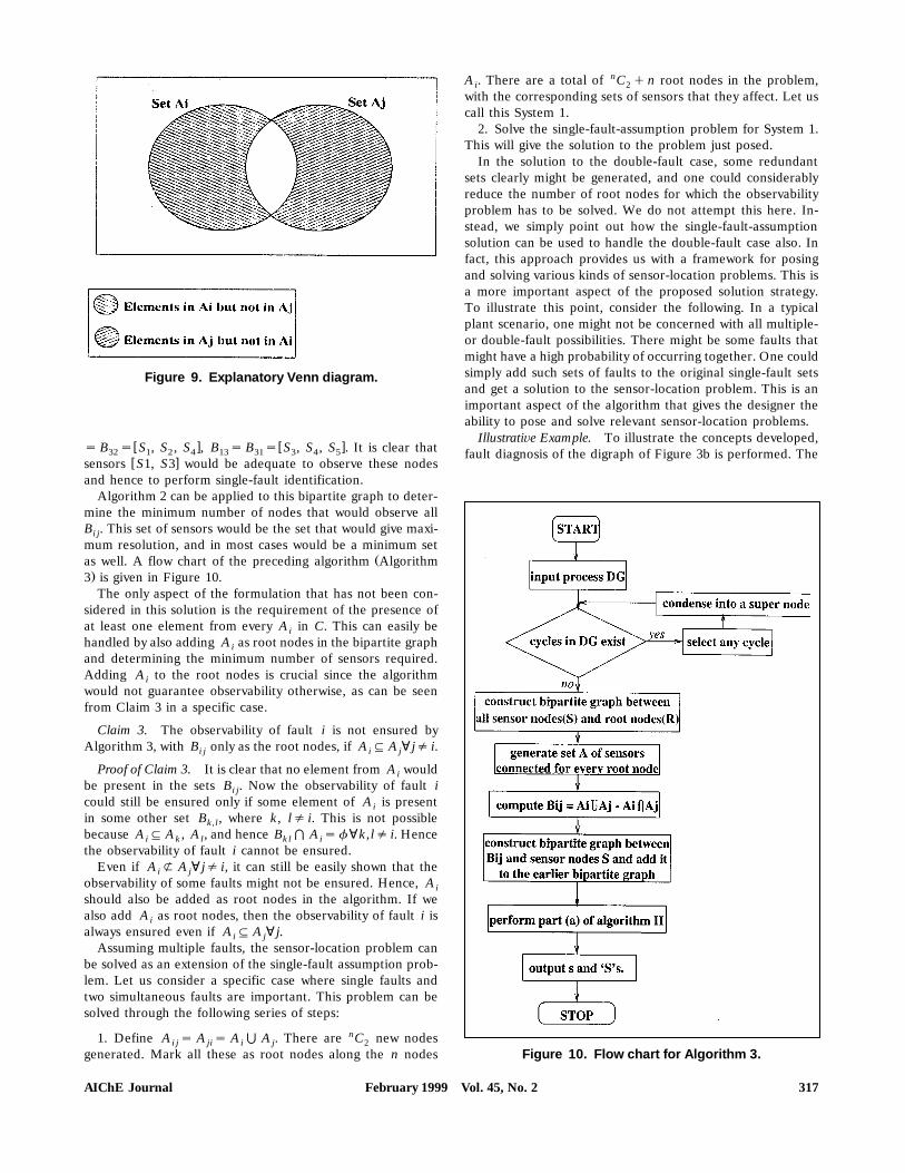
Figure 9. Explanatory Venn diagram.
w x w xs B s S , S , S , B s B s S , S , S . It is clear that32 1 2 4 13 31 3 4 5w xsensors S1, S3 would be adequate to observe these nodes
and hence to perform single-fault identification.Algorithm 2 can be applied to this bipartite graph to deter-
mine the minimum number of nodes that would observe allB . This set of sensors would be the set that would give maxi-i jmum resolution, and in most cases would be a minimum set
Žas well. A flow chart of the preceding algorithm Algorithm.3 is given in Figure 10.The only aspect of the formulation that has not been con-
sidered in this solution is the requirement of the presence ofat least one element from every A in C. This can easily beihandled by also adding A as root nodes in the bipartite graphiand determining the minimum number of sensors required.Adding A to the root nodes is crucial since the algorithmiwould not guarantee observability otherwise, as can be seenfrom Claim 3 in a specific case.
Claim 3. The observability of fault i is not ensured byAlgorithm 3, with B only as the root nodes, if A : A ; j/ i.i j i j
Proof of Claim 3. It is clear that no element from A wouldibe present in the sets B . Now the observability of fault ii jcould still be ensured only if some element of A is presentiin some other set B , where k, l/ i. This is not possiblek, lbecause A : A , A , and hence B F A sf ;k,l/ i. Hencei k l kl ithe observability of fault i cannot be ensured.
Even if A o A ; j/ i, it can still be easily shown that thei jobservability of some faults might not be ensured. Hence, Aishould also be added as root nodes in the algorithm. If wealso add A as root nodes, then the observability of fault i isialways ensured even if A : A ; j.i j
Assuming multiple faults, the sensor-location problem canbe solved as an extension of the single-fault assumption prob-lem. Let us consider a specific case where single faults andtwo simultaneous faults are important. This problem can besolved through the following series of steps:
1. Define A s A s A D A . There are nC new nodesi j ji i j 2generated. Mark all these as root nodes along the n nodes
A . There are a total of nC q n root nodes in the problem,i 2with the corresponding sets of sensors that they affect. Let uscall this System 1.
2. Solve the single-fault-assumption problem for System 1.This will give the solution to the problem just posed.
In the solution to the double-fault case, some redundantsets clearly might be generated, and one could considerablyreduce the number of root nodes for which the observabilityproblem has to be solved. We do not attempt this here. In-stead, we simply point out how the single-fault-assumptionsolution can be used to handle the double-fault case also. Infact, this approach provides us with a framework for posingand solving various kinds of sensor-location problems. This isa more important aspect of the proposed solution strategy.To illustrate this point, consider the following. In a typicalplant scenario, one might not be concerned with all multiple-or double-fault possibilities. There might be some faults thatmight have a high probability of occurring together. One couldsimply add such sets of faults to the original single-fault setsand get a solution to the sensor-location problem. This is animportant aspect of the algorithm that gives the designer theability to pose and solve relevant sensor-location problems.
Illustrati®e Example. To illustrate the concepts developed,fault diagnosis of the digraph of Figure 3b is performed. The
Figure 10. Flow chart for Algorithm 3.
February 1999 Vol. 45, No. 2AIChE Journal 317
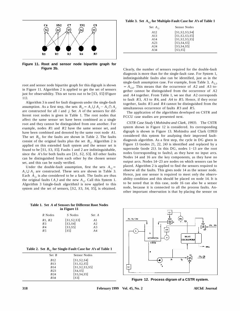
Figure 11. Root and sensor node bipartite graph forFigure 3b.
root and sensor node bipartite graph for this digraph is shownin Figure 11. Algorithm 2 is applied to get the set of sensors
w x Žjust for observability. This set turns out to be S3, S5 Figure.11 .Algorithm 3 is used for fault diagnosis under the single-fault
assumption. As a first step, the sets B s A D A y A F Ai j i j i jare constructed for all i and j. Set A of the sensors for dif-ferent root nodes is given in Table 1. The root nodes thataffect the same sensor set have been combined as a singleroot and they cannot be distinguished from one another. Forexample, nodes R1 and R2 have the same sensor set, andhave been combined and denoted by the same root node A1.The set B for the faults are shown in Table 2. The faultsi jconsist of the original faults plus the set B . Algorithm 2 isi japplied on this extended fault system and the sensor set is
w xfound to be S1, S3, S5 . Faults 1 and 2 are indistinguishable,w xsince the A’s for both faults are S1, S2, S3 . All other faults
can be distinguished from each other by the chosen sensorset, and this can be easily verified.
Under the double-fault assumption, first the sets A si jA D A are constructed. These sets are shown in Table 3.i jEach A is also considered to be a fault. The faults are thusi j
Ž .the original faults A and the new A . Call this System 1.i i jŽ .Algorithm 3 single-fault algorithm is now applied to this
w xsystem and the set of sensors, S2, S3, S4, S5 , is obtained.
Table 1. Set A of Sensors for Different Root Nodesin Figure 11
R Nodes S Nodes Set A
w xR1, R2 S1,S2,S3 A1w xR3 S3,S4 A2w xR4 S3,S5 A3w xR5 S5 A4
Table 2. Set B for Single-Fault Case for A’s of Table 1i j
Set B Sensor Nodesw xB12 S1,S2,S4w xB13 S1,S2,S5w xB14 S1,S2,S3,S5w xB23 S4,S5w xB24 S3,S4,S5w xB34 S3
Table 3. Set A for Multiple-Fault Case for A’s of Table 1i j
Set A Sensor Nodesi j
w xA12 S1,S2,S3,S4w xA13 S1,S2,S3,S5w xA14 S1,S2,S3,S5w xA23 S3,S4,S5w xA24 S3,S4,S5w xA34 S3,S5
Clearly, the number of sensors required for the double-faultdiagnosis is more than for the single-fault case. For System 1,indistinguishable faults also can be identified, just as in thesingle-fault assumption case. For example, from Table 3, A2,3s A . This means that the occurrence of A2 and A3 to-2,4gether cannot be distinguished from the occurrence of A2and A4 together. From Table 1, we see that A2 correspondsto fault R3, A3 to R4, and A4 to R5. Hence, if they occurtogether, faults R3 and R4 cannot be distinguished from thesimultaneous occurrence of faults R3 and R5.
The application of the algorithms developed on CSTR andFCCU case studies are presented next.
Ž .CSTR Case Study Mohindra and Clark, 1993 . The CSTRsystem shown in Figure 12 is considered. Its corresponding
Ž .digraph is shown in Figure 13. Mohindra and Clark 1993considered this system for analyzing their improved fault-diagnosis algorithm. As a first step, the cycle in DG given in
Ž .Figure 13 nodes 21, 22, 24 is identified and replaced by aŽ .supernode node 21 . In this DG, nodes 1]13 are the root
Ž .nodes corresponding to faults , as they have no input arcs.Nodes 14 and 16 are the key components, as they have nooutput arcs. Nodes 14]23 are nodes on which sensors can beplaced. Algorithm 2 is applied to find the sensors required toobserve all the faults. This gives node 14 as the sensor node.Hence, just one sensor is required to meet only the observ-ability condition and this should be placed on node 14. It isto be noted that in this case, node 16 can also be a sensornode, because it is connected to all the process faults. An-other important observation is that by placing the sensor on
Figure 12. Process digram of a CSTR system.
February 1999 Vol. 45, No. 2 AIChE Journal318
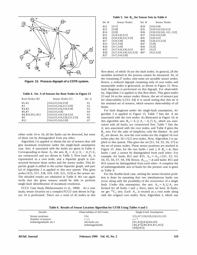
Figure 13. Process digraph of a CSTR system.
Table 4. Set A of Sensors for Root Nodes in Figure 13
Ž . Ž .Root Nodes R Sensor Nodes S Set A
w xR1, R2 S14,S15,S16,S19 A1w xR3 S14,S15,S16,S17,S19 A2w xR4, R5 S14,S15,S16,S18,S19 A3w xR6, R7 S14,S15,S16 A4w xR8, R10, R11, R13 S14,S15,S16,S20,S21 A5w xR9 S14,S15,S16,S20,S21,S23 A6w xR12 S14,S15,S16,S20 A7
either node 14 or 16, all the faults can be detected, but noneof them can be distinguished from any other.
Algorithm 3 is applied to obtain the set of sensors that willgive maximum resolution under the single-fault assumptioncase. Sets A associated with the faults are given in Table 4.Corresponding to these A , the sets B s A D A y A F Ai i j i j i jare constructed and are shown in Table 5. Now each B isi jrepresented as a root node, and a bipartite graph is con-structed between these nodes and the sensor nodes. This bi-partite graph is added to the earlier bipartite graph, and partŽ .a of Algorithm 2 is applied to this new system. This gives
w xnodes S15, S17, S18, S19, S20, S21, S23 as the sensor set.The detailed results are tabulated in Table 6. We can againverify that the given sensors would be able to performsingle-fault identification of maximum resolution.
Ž .FCCU Case Study Mylaraswamy et al., 1994 . As a casestudy, sensor location on a complex FCCU unit shown in Fig-ure 14 is performed. There are a total of 43 nodes in this
Table 5. Set B for Sensor Sets in Table 4i j
Set B Sensor Nodes Set B Sensor Nodesw x w xB12 S17 B34 S18,S19w x w xB13 S18 B35 S18,S19,S20,S21w x w xB14 S19 B36 S18,S19,S20, S21, S23w x w xB15 S19,S20,S21 B37 S18,S19,S20w x w xB16 S19,S20,S21,S23 B45 S20,S21w x w xB17 S19,S20 B46 S20,S21,S23w x w xB23 S17,S18 B47 S20w x w xB24 S17,S19 B56 S23w x w xB25 S17,S19,S20,S21 B57 S21w x w xB26 S17,S19,S20,S21,S23 B67 S21,S23w xB27 S17,S19,S20
flow sheet, of which 16 are the fault nodes. In general, all thevariables involved in the process cannot be measured. So, ofthe remaining 27 nodes, only some are possible sensor nodes.Hence, a reduced digraph consisting only of root nodes andmeasurable nodes is generated, as shown in Figure 15. Now,fault diagnosis is performed on this digraph. For observabil-ity, Algorithm 2 is applied to this flow sheet. This gives nodesS3 and S4 as the sensor nodes. Hence, the set of sensors just
w xfor observability is S3, S4 . It is worth noting that this set isthe minimal set of sensors, which ensures observability of allfaults.
For fault diagnosis under the single-fault assumption, Al-gorithm 3 is applied to Figure 15. Table 7 lists the A setassociated with the root nodes. As illustrated in Figure 10, inthis algorithm sets B s A D A y A F A , which are asso-i j i j i jciated with all faults, are constructed first. Table 7 lists theA sets associated with the root nodes, and Table 8 gives theiB sets. For the sake of simplicity, only the distinct As andi jB are shown. So, now the root nodes are the original 16 rooti jnodes plus the 16=15r2 new nodes. Now, Algorithm 2 is ap-
w xplied to this system. This gives the set S1, S4, S5, S6, S7 asthe set of sensor nodes. These sensor positions are marked inFigure 15. Also, for the two faults i and j, if B sf, theni jfaults i and j cannot be distinguished from each other. For
wexample, for faults R11 and R15, A s A s S1, S2, S3,11 15xS4, S5, S6, S7, S8, S9 . Hence, B sf and faults R11 and11,15
R15 cannot be distinguished from each other. A complete listof indistinguishable sets of faults for the present case is givenin Table 9.
For the double-fault case, solving the sensor-location prob-lem is done by assuming that two simultaneous faults canoccur along with the possibility of the occurrence of a singlefault. Under this assumption, the sets A s A D A arei j i jformed for all faults i and j. Here, since we have 16 faults,we get 16C sets. Each A is treated as a root node along2 i jwith the original root nodes. Now, Algorithm 3, which was
Table 6. Results of Sensor Location Algorithm for CSTR Using Tables 4 and 5
Details Observability of All Faults Single-Fault Assumption
Sensor positions S14 S15,S17,S18,S19,S20,S21,S23Number of sensors cs1 ss7
w x w x w xIndistinguishable set I All faults are R1, R2 , R3 , R4, R5w x w xindistinguishable R6, R7 , R8, R10, R11, R13w x w xR9 , R12
February 1999 Vol. 45, No. 2AIChE Journal 319
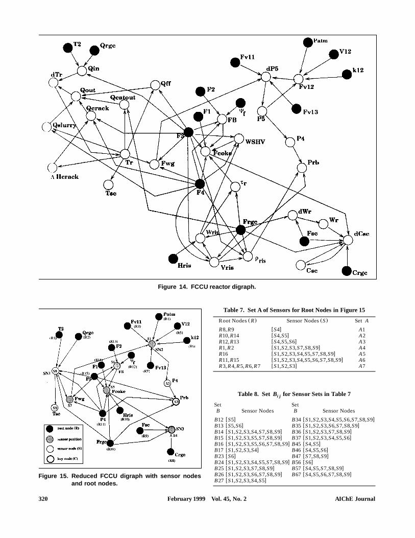
Figure 14. FCCU reactor digraph.
Figure 15. Reduced FCCU digraph with sensor nodesand root nodes.
Table 7. Set A of Sensors for Root Nodes in Figure 15
Ž . Ž .Root Nodes R Sensor Nodes S Set A
w xR8, R9 S4 A1w xR10, R14 S4,S5 A2w xR12, R13 S4,S5,S6 A3w xR1, R2 S1,S2,S3,S7,S8,S9 A4w xR16 S1,S2,S3,S4,S5,S7,S8,S9 A5w xR11, R15 S1,S2,S3,S4,S5,S6,S7,S8,S9 A6w xR3, R4, R5, R6, R7 S1,S2,S3 A7
Table 8. Set B for Sensor Sets in Table 7i j
Set SetB Sensor Nodes B Sensor Nodes
w x w xB12 S5 B34 S1,S2,S3,S4,S5,S6,S7,S8,S9w x w xB13 S5,S6 B35 S1,S2,S3,S6,S7,S8,S9w x w xB14 S1,S2,S3,S4,S7,S8,S9 B36 S1,S2,S3,S7,S8,S9w x w xB15 S1,S2,S3,S5,S7,S8,S9 B37 S1,S2,S3,S4,S5,S6w x w xB16 S1,S2,S3,S5,S6,S7,S8,S9 B45 S4,S5w x w xB17 S1,S2,S3,S4 B46 S4,S5,S6w x w xB23 S6 B47 S7,S8,S9w x w xB24 S1,S2,S3,S4,S5,S7,S8,S9 B56 S6w x w xB25 S1,S2,S3,S7,S8,S9 B57 S4,S5,S7,S8,S9w x w xB26 S1,S2,S3,S6,S7,S8,S9 B67 S4,S5,S6,S7,S8,S9w xB27 S1,S2,S3,S4,S5
February 1999 Vol. 45, No. 2 AIChE Journal320
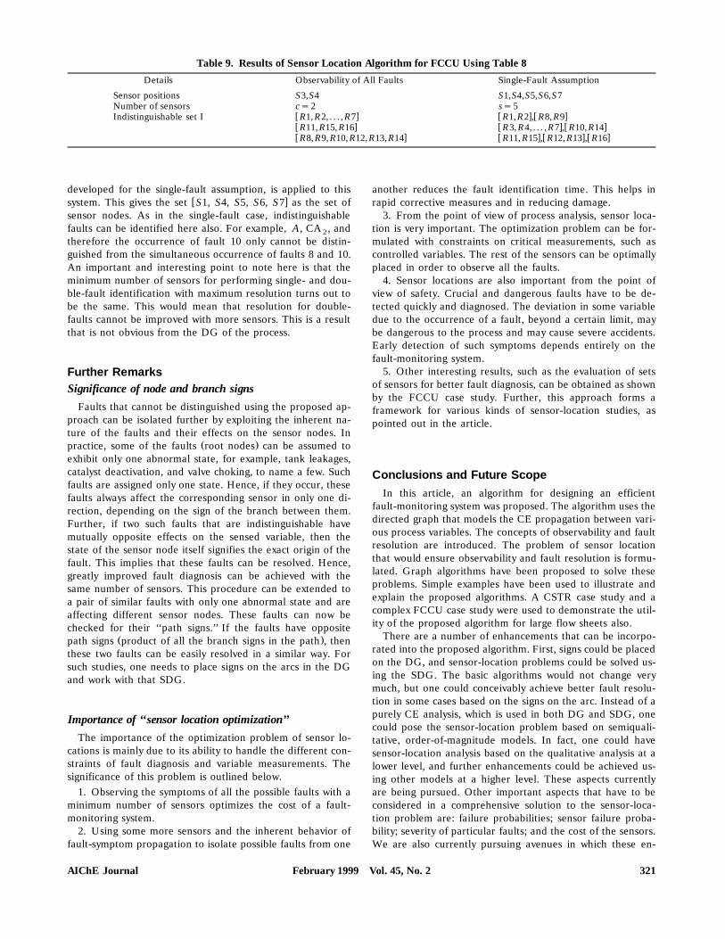
Table 9. Results of Sensor Location Algorithm for FCCU Using Table 8
Details Observability of All Faults Single-Fault Assumption
Sensor positions S3,S4 S1,S4,S5,S6,S7Number of sensors cs2 ss5
w x w x w xIndistinguishable set I R1, R2, . . . , R7 R1, R2 , R8, R9w x w x w xR11, R15, R16 R3, R4, . . . , R7 , R10, R14w x w x w x w xR8, R9, R10, R12, R13, R14 R11, R15 , R12, R13 , R16
developed for the single-fault assumption, is applied to thisw xsystem. This gives the set S1, S4, S5, S6, S7 as the set of
sensor nodes. As in the single-fault case, indistinguishablefaults can be identified here also. For example, A, CA , and2therefore the occurrence of fault 10 only cannot be distin-guished from the simultaneous occurrence of faults 8 and 10.An important and interesting point to note here is that theminimum number of sensors for performing single- and dou-ble-fault identification with maximum resolution turns out tobe the same. This would mean that resolution for double-faults cannot be improved with more sensors. This is a resultthat is not obvious from the DG of the process.
Further RemarksSignificance of node and branch signs
Faults that cannot be distinguished using the proposed ap-proach can be isolated further by exploiting the inherent na-ture of the faults and their effects on the sensor nodes. In
Ž .practice, some of the faults root nodes can be assumed toexhibit only one abnormal state, for example, tank leakages,catalyst deactivation, and valve choking, to name a few. Suchfaults are assigned only one state. Hence, if they occur, thesefaults always affect the corresponding sensor in only one di-rection, depending on the sign of the branch between them.Further, if two such faults that are indistinguishable havemutually opposite effects on the sensed variable, then thestate of the sensor node itself signifies the exact origin of thefault. This implies that these faults can be resolved. Hence,greatly improved fault diagnosis can be achieved with thesame number of sensors. This procedure can be extended toa pair of similar faults with only one abnormal state and areaffecting different sensor nodes. These faults can now bechecked for their ‘‘path signs.’’ If the faults have opposite
Ž .path signs product of all the branch signs in the path , thenthese two faults can be easily resolved in a similar way. Forsuch studies, one needs to place signs on the arcs in the DGand work with that SDG.
Importance of ‘‘ sensor location optimization’’The importance of the optimization problem of sensor lo-
cations is mainly due to its ability to handle the different con-straints of fault diagnosis and variable measurements. Thesignificance of this problem is outlined below.
1. Observing the symptoms of all the possible faults with aminimum number of sensors optimizes the cost of a fault-monitoring system.
2. Using some more sensors and the inherent behavior offault-symptom propagation to isolate possible faults from one
another reduces the fault identification time. This helps inrapid corrective measures and in reducing damage.
3. From the point of view of process analysis, sensor loca-tion is very important. The optimization problem can be for-mulated with constraints on critical measurements, such ascontrolled variables. The rest of the sensors can be optimallyplaced in order to observe all the faults.
4. Sensor locations are also important from the point ofview of safety. Crucial and dangerous faults have to be de-tected quickly and diagnosed. The deviation in some variabledue to the occurrence of a fault, beyond a certain limit, maybe dangerous to the process and may cause severe accidents.Early detection of such symptoms depends entirely on thefault-monitoring system.
5. Other interesting results, such as the evaluation of setsof sensors for better fault diagnosis, can be obtained as shownby the FCCU case study. Further, this approach forms aframework for various kinds of sensor-location studies, aspointed out in the article.
Conclusions and Future ScopeIn this article, an algorithm for designing an efficient
fault-monitoring system was proposed. The algorithm uses thedirected graph that models the CE propagation between vari-ous process variables. The concepts of observability and faultresolution are introduced. The problem of sensor locationthat would ensure observability and fault resolution is formu-lated. Graph algorithms have been proposed to solve theseproblems. Simple examples have been used to illustrate andexplain the proposed algorithms. A CSTR case study and acomplex FCCU case study were used to demonstrate the util-ity of the proposed algorithm for large flow sheets also.
There are a number of enhancements that can be incorpo-rated into the proposed algorithm. First, signs could be placedon the DG, and sensor-location problems could be solved us-ing the SDG. The basic algorithms would not change verymuch, but one could conceivably achieve better fault resolu-tion in some cases based on the signs on the arc. Instead of apurely CE analysis, which is used in both DG and SDG, onecould pose the sensor-location problem based on semiquali-tative, order-of-magnitude models. In fact, one could havesensor-location analysis based on the qualitative analysis at alower level, and further enhancements could be achieved us-ing other models at a higher level. These aspects currentlyare being pursued. Other important aspects that have to beconsidered in a comprehensive solution to the sensor-loca-tion problem are: failure probabilities; sensor failure proba-bility; severity of particular faults; and the cost of the sensors.We are also currently pursuing avenues in which these en-
February 1999 Vol. 45, No. 2AIChE Journal 321
hancements can be integrated into the solution to thesensor-location problem proposed in this article.
Notationcsnumber of sensors for fault observabilityIsset of indistinguishable faults
Nsnumber of root nodes in the DGOsD Ai iSssensor nodessnumber of sensors for highest fault resolution
Literature CitedAli, Y., and S. Narasimhan, ‘‘Sensor Network Design for Maximizing
Ž . Ž .Reliability of Linear Processes,’’ AIChE J., 39 5 , 820 1993 .Ali, Y., and S. Narasimhan, ‘‘Redundant Sensor Network Design for
Ž . Ž .Linear Processes,’’ AIChE J., 41 10 , 2237 1995 .Ali, Y., and S. Narasimhan, ‘‘Sensor Network Design for Maximizing
Ž . Ž .Reliability of Bilinear Processes,’’ AIChE J., 42 9 , 2563 1996 .Chang, C. C., and C. C. Yu, ‘‘On-Line Fault Diagnosis using the
Ž .Signed Directed Graph,’’ Ind. Eng. Chem. Res., 29, 1290 1990 .Chang, C. C., K. N. Mah, and C. S. Tsai, ‘‘A Simple Design Strategy
Ž . Ž .for Fault Monitoring Systems,’’ AIChE J., 39 7 , 1146 1993 .Deo, N., Graph Theory with Applications to Engineering and Computer
Ž .Science, Prentice Hall of India, New Delhi 1997 .
February 1999322
Iri, M., K. Aoki, E. O’Shima, and H. Matsuyama, ‘‘An Algorithm forDiagnosis of System Failures in Chemical Processes,’’ Comput.
Ž .Chem. Eng., 3, 489 1979 .Kramer, M. A., and B. L. Palowitch, Jr., ‘‘A Rule-Based Approach to
Ž .Fault Diagnosis using the Signed Directed Graph,’’ AIChE J., 33 7 ,Ž .1067 1987 .
Lambert, H. E., ‘‘Fault Trees for Locating Sensors in Process Sys-Ž .tems,’’ Chem. Eng. Prog., 81 Aug. 1977 .
Madron, F., and V. Veverka, ‘‘Optimal Selection of Measuring PointsŽ . Ž .in Complex Plants by Linear Models,’’ AIChE J., 38 2 , 227 1992 .
Mohindra, S., and P. A. Clark, ‘‘A Distributed Fault DiagnosisMethod Based on Digraph Models: Steady-State Analysis,’’ Com-
Ž . Ž .put. Chem. Eng., 17 2 , 193 1993 .Mylaraswamy, D., S. N. Kavuri, and V. Venkatasubramanian, ‘‘Sys-
tematic Development of Causal Digraph Models for ChemicalŽ .Processes,’’ AIChE Meeting, San Francisco 1994 .
O’Shima, E., J. Shiozaki, H. Matsuyama, and M. Iri, ‘‘An ImprovedAlgorithm for Diagnosis of System Failures in the Chemical Pro-
Ž .cess,’’ Comput. Chem. Eng., 9, 285 1985 .Parker, R. G., and R. L. Rardin, Discrete Optimization, Academic
Ž .Press, San Diego 1988 .Peng, Y., and J. A. Reggia, Abducti®e Inference Models for Diagnostic
Ž .Problem Sol®ing, Springer-Verlag, New York 1990 .
Manuscript recei®ed May 27, 1998, and re®ision recei®ed Sept. 14, 1998.
Vol. 45, No. 2 AIChE Journal