Localized and Precise Boundary Detection in 3-D Wireless Sensor Networks

This article has been accepted for inclusion in a future issue of this journal. Content is final as presented, with the exception of pagination.

IEEE/ACM TRANSACTIONS ON NETWORKING 1

Localized and Precise Boundary Detection in 3-DWireless Sensor Networks

Hongyu Zhou, Student Member, IEEE, Su Xia, Member, IEEE, Miao Jin, and Hongyi Wu, Member, IEEE

Abstract—This research focuses on distributed and localized al-gorithms for precise boundary detection in 3-D wireless networks.Our objectives are twofold. First, we aim to identify the nodes onthe boundaries of a 3-D network, which serve as a key attributethat characterizes the network, especially in such geographic ex-ploration tasks as terrain and underwater reconnaissance. Second,we construct locally planarized 2-manifold surfaces for inner andouter boundaries in order to enable available graph theory tools tobe applied on 3-D surfaces, such as embedding, localization, parti-tion, and greedy routing among many others. To achieve the firstobjective, we propose a Unit Ball Fitting (UBF) algorithm that dis-covers a majority of boundary nodes, followed by a refinementalgorithm, named Isolated Fragment Filtering (IFF), to removeisolated nodes that are misinterpreted as boundary nodes. Basedon the identified boundary nodes, we develop an algorithm thatconstructs a locally planarized triangular mesh surface for each3-D boundary. Our proposed scheme is localized, requiring infor-mation within 1-hop neighborhood only. We further extend theschemes for online boundary detection in mobile sensor networksaiming to achieve low overhead. Our simulation and experimentalresults demonstrate that the proposed algorithms can effectivelyidentify boundary nodes and surfaces, even under high measure-ment errors.

Index Terms—Boundary detection, triangulation, wirelesssensor networks.

I. INTRODUCTION

M ANY wireless networks exhibit substantial random-ness, due to the lack of precise nodal deployment and

the nondeterministic failures and channel dynamics. Therefore,the final formation of a wireless network heavily depends onits underlying environment. Consequently, there is a primaryinterest to discover the unknown geometry and topology of awireless network formation (or a subnetwork formation), whichprovide salient information for understanding its environmentand for efficient operation of the network itself. In particular,boundary is one of the key attributes that characterize the net-

Manuscript received February 25, 2014; revised June 10, 2014; accepted July11, 2014; approved by IEEE/ACM TRANSACTIONS ON NETWORKING Editor X.Wang. Part of this work was presented at the IEEE International Conference onDistributed Computing Systems (ICDCS), Genova, Italy, June 21–25, 2010.H. Zhou was with the Center for Advanced Computer Studies (CACS), Uni-

versity of Louisiana at Lafayette, Lafayette, LA 70503 USA. He is now withEpic Systems, Verona, WI 53593 USA (e-mail: [email protected]).S. Xia was with the Center for Advanced Computer Studies (CACS), Univer-

sity of Louisiana at Lafayette, Lafayette, LA 70503 USA. He is now with CiscoSystems, Inc., San Jose, CA 95134 USA (e-mail: [email protected]).M. Jin and H. Wu are with the Center for Advanced Computer Studies

(CACS), University of Louisiana at Lafayette, Lafayette, LA 70503 USA(e-mail: [email protected]; [email protected]).Color versions of one or more of the figures in this paper are available online

at http://ieeexplore.ieee.org.Digital Object Identifier 10.1109/TNET.2014.2344663

work in two- (2-D) or three-dimensional (3-D) space, especiallyin such geographic exploration tasks as terrain and underwaterreconnaissance.

A. Related Work

The quest for efficient boundary detection in wireless net-works has led to two research thrusts outlined here.Detection of Event Boundary: The investigation on boundary

detection started from the estimation and localization of eventsin sensor networks. The spatially distributed sensors usuallyreport different measurements in respond to an event. For ex-ample, upon a fire, the sensors located in the fire are likely de-stroyed (and thus resulting a void area of failed nodes), whilethe sensors close to the fire region measure higher temperatureand smoke density than the faraway sensors do. Boundary de-tection is to delineate the regions of distinct behavior in a sensornetwork [1].Achieving accurate detection of event boundary is chal-

lenging because the sampling density is limited, the sensorreadings are noisy, the delivery of sensor data is unreliable,and the computation power of individual sensors is extremelylow [1], [2]. To this end, a series of studies has been carriedout to explore efficient information processing and modelingtechniques to analyze sensor data in order to estimate theboundary of events [1]–[5].Due to inevitable errors in raw sensor data, these ap-

proaches do not yield precise boundary. Instead, they aim ata close-enough estimation that correctly identifies the eventsfrontier, based on either global or local data collected from aset of sensors.Detection of Network Boundary: Besides the research

discussed above that is mainly from the data processing per-spective, interests are also developed to precisely locate theboundary of the network based on geometric or topology infor-mation of a wireless network. Noise in sensor data is no longera concern here because such boundary detection is not basedon sensor measurement. However, new challenges arise dueto the required accuracy of the identified boundary, especiallyin networks with complex inner boundary (i.e., “holes”) or inhigh-dimensional space.Most proposed network boundary detection algorithms are

based on 2-D graphic tools. For example, Voronoi diagrams areemployed in [6] and [7] to discover coverage holes in sensornetworks. Delaunay triangulation is adopted in [8] to identifycommunication voids. In contrast to [6]–[8] that exploit sensorpositions, two distributed algorithms are proposed in [9] by uti-lizing distance and/or angle information between nodes to dis-cover coverage boundary.

1063-6692 © 2014 IEEE. Personal use is permitted, but republication/redistribution requires IEEE permission.See http://www.ieee.org/publications_standards/publications/rights/index.html for more information.


2 IEEE/ACM TRANSACTIONS ON NETWORKING

In [10], an algebraic topological invariant called homologyis computed to detect holes. The algorithm is generally appli-cable to networks in any dimensional space. However, it is acentralized approach, and there is significant challenge to de-centralize its computation as pointed out in [10]. In [11], theisosets (each of which consists of nodes with the same hop dis-tance to a beacon node) are identified. The disconnection in anisoset indicates the boundary nodes of holes. Multiple beaconscan be employed to locate the boundary nodes at different di-rections of a hole. This approach does not guarantee to discoverthe complete boundary of every hole. Higher accuracy can beachieved if more beacons are employed or when the networkis denser. Reference [12] introduces a deterministic algorithmfor boundary detection. It searches for a special subgraph struc-ture, called m-flower, which is bounded by a circle. Once anm-flower is identified, the algorithm can subsequently find theboundary nodes through a number of iterations of augmenta-tion of the circle. However, not every graph has an m-flowerstructure. Therefore, the algorithm may fail especially when thenodal density is low. In [13], a shortest path tree is built to findthe shortest circle, which is then refined to discover the tightboundaries of the inner holes.All of the network boundary detection approaches discussed

above are developed for networks in 2-D space. Except for [10],which is centralized, none of them can be readily applied to3-D networks since higher-dimension space introduces signifi-cant complexity in searching for boundaries, and many topolog-ical and geometrical tools cannot be extended from 2-D to 3-D.Note that if global coordinates are available, boundary detec-tion would become straightforward. However, this approach isoften overkilling because the process of establishing global co-ordinates itself results in significant computation and commu-nication overhead [14]. In addition, while boundary extractionhas been extensively studied in 3-D imaging, the algorithms de-veloped therein always assume grid-like 3-D pixels as inputs,which are in sharp contrast to network settings where nodes arerandomly distributed, and thus are not applicable in 3-D wire-less networks.This work (partially presented in [15]) proposes the first

algorithms for efficiently discovering boundary nodes andconstructing boundary surface in 3-D wireless sensor networks.Following [15], several relevant research works have beencarried out recently. For example, an effective algorithm isproposed in [16] to timely track dynamic network boundaries.It transforms a notched surface into a convex one to supportof fast online boundary detection. However, the performanceof the algorithm is determined by two important parametersrequired by the transformation. Unfortunately, both of themare model-dependent. Different models have different optimalparameters for achieving the best results. More discussionand comparison will be presented in Section V. It deals withboundary nodes only, but not surface. References [17] and [18]aim to address the 3-D wireless boundary detection problembased on connectivity only. In [17], an algorithm called CABETis proposed. It first identifies a set of boundary nodes based onthe assumption that a boundary node has less neighbors thanits internal counterpart. Then, three types of critical boundarynodes (i.e., convex, concave, and saddle nodes) are selected to

depict the geometric features of the 3-D sensor network, basedon which closed boundary surfaces are constructed. CABET iseffective when the sensors are uniformly distributed, yieldingaccurate boundary nodes and boundary surfaces. When itcomes to nonuniform networks, CABET often becomeserror-prone. An algorithm dubbed “Cococut” is introduced in[18]. It overcomes this problem by constructing a tetrahedralstructure to delineate the approximate geometry of the 3-Dsensor network, which is independent to nodal distribution. Aset of sealed triangular boundary surfaces is produced basedon this structure to separate nonboundary nodes and boundarynode candidates. The former are hollowed out immediately,while the latter are further refined to yield the final boundarynodes and fine-grained boundary surfaces. However, the con-nectivity-based approaches cannot differentiate nodes within 1hop, and thus are less accurate compared to the performance ofmethods based on distance or coordinates.

B. Our Contribution

There are increasing interests in 3-D wireless networks, withseveral areas such as routing [19]–[24], localization [14], [25],nodal placement [26], [27], physical-layer investigation [28],and applications [28], [29] being explored recently. This re-search aims to develop distributed and localized algorithms forprecise boundary detection in 3-D wireless networks. Our ob-jectives are twofold.1) First, we aim to identify the nodes on the boundaries of a3-D network based on local information [see Fig. 1(b) forexample].

2) Second, we construct locally planarized 2-manifold sur-faces for inner and outer boundaries [as shown in Fig. 1(f)].

To achieve the first objective, we propose a Unit Ball Fit-ting (UBF) algorithm that discovers a set of boundary nodes,followed by a refinement algorithms, named Isolated FragmentFiltering (IFF), which removes isolated nodes that are misin-terpreted as boundary nodes by UBF. Our proposed schemeis localized, requiring information within 1-hop neighborhoodonly. This quality is highly desired to enable fast and low-costboundary detection.The boundary nodes are discrete. They serve as sample points

that depict the network boundaries. However, many applicationsdesire not only such discrete points, but also closed boundarysurfaces, especially locally planarized 2-manifold in order toapply available graph theory tools on 3-D surfaces, such asembedding, localization, partition, and greedy routing amongmany others. In this research, we develop an algorithm thatconstructs locally planarized triangular meshes on the identified3-D boundaries. We adopt the method proposed in [30] that pro-duces a planar subgraph in 2-D, and extend it to 3-D surfaces toachieve complete triangulation without degenerated edges. Thealgorithm is localized and based on connectivity only.We further extend the proposed methods for dynamic sensor

networks where sensors are mobile. We propose an efficientupdating scheme to reduces the number of nodes running UBFwithout degrading the performance of the online boundarydetection and to maintain the surface triangle mesh after it isconstructed initially, with high efficiency in terms of time andenergy.


ZHOU et al.: LOCALIZED AND PRECISE BOUNDARY DETECTION IN 3-D WIRELESS SENSOR NETWORKS 3

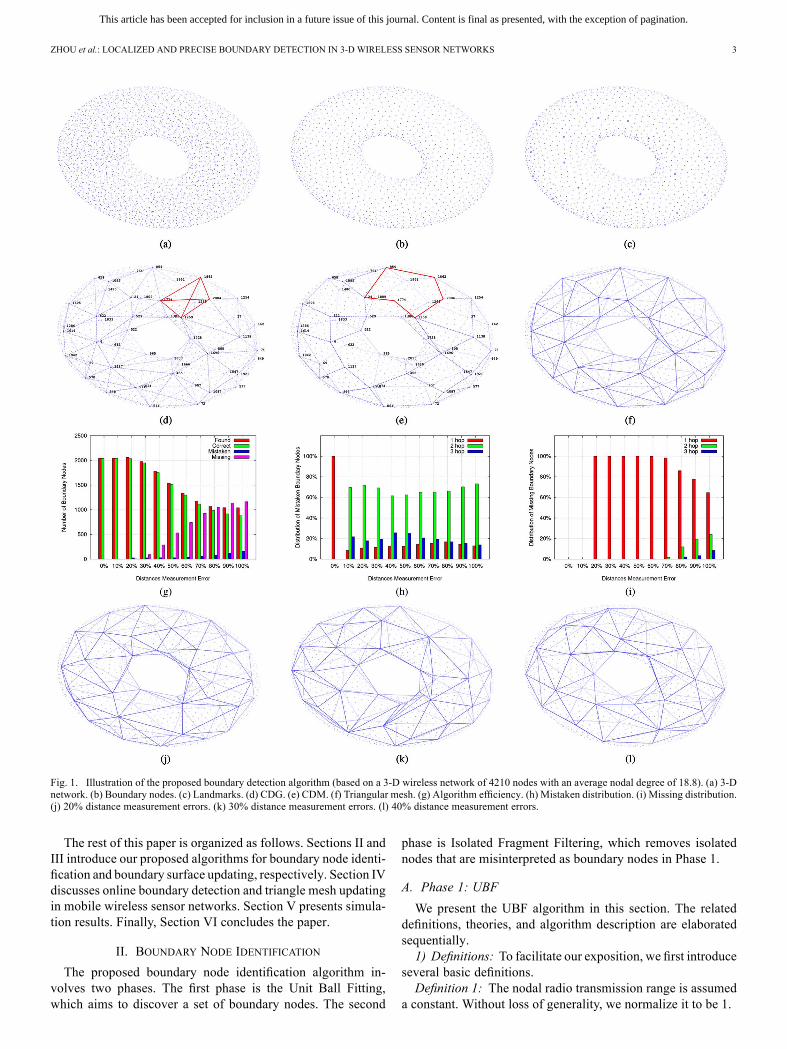
Fig. 1. Illustration of the proposed boundary detection algorithm (based on a 3-D wireless network of 4210 nodes with an average nodal degree of 18.8). (a) 3-Dnetwork. (b) Boundary nodes. (c) Landmarks. (d) CDG. (e) CDM. (f) Triangular mesh. (g) Algorithm efficiency. (h) Mistaken distribution. (i) Missing distribution.(j) 20% distance measurement errors. (k) 30% distance measurement errors. (l) 40% distance measurement errors.

The rest of this paper is organized as follows. Sections II andIII introduce our proposed algorithms for boundary node identi-fication and boundary surface updating, respectively. Section IVdiscusses online boundary detection and triangle mesh updatingin mobile wireless sensor networks. Section V presents simula-tion results. Finally, Section VI concludes the paper.

II. BOUNDARY NODE IDENTIFICATION

The proposed boundary node identification algorithm in-volves two phases. The first phase is the Unit Ball Fitting,which aims to discover a set of boundary nodes. The second

phase is Isolated Fragment Filtering, which removes isolatednodes that are misinterpreted as boundary nodes in Phase 1.

A. Phase 1: UBF

We present the UBF algorithm in this section. The relateddefinitions, theories, and algorithm description are elaboratedsequentially.1) Definitions: To facilitate our exposition, we first introduce

several basic definitions.Definition 1: The nodal radio transmission range is assumed

a constant. Without loss of generality, we normalize it to be 1.



Definition 2: The nodal density, denoted by , is the averagenumber of nodes in a unit volume.Definition 3: A well-connected network is a network where:

1) no nodes are isolated; and 2) there are no degenerated linesegments. In other words, given a line segment between twonodes, e.g., Nodes and , there must be at least one node whosedistances to Nodes and are less than , wheredenotes the distance between Nodes and .We consider well-connected networks only in this work

because the isolated nodes and degenerated line segmentsare swingable, causing ambiguity in boundary definition anddetection.Definition 4: A unit ball is a ball with a radius of ,

where is an arbitrarily small constant.Definition 5: An empty unit ball is a unit ball with no nodes

located inside.Definition 6: We say a unit ball touches a node if the node is

on the surface of the ball.Definition 7: A hole is an empty space that is greater than a

unit ball. The space outside the network is treated as a specialhole.With the above definitions, we next discuss the motivations

to develop the UBF algorithm and the theories that prove itscorrectness and computing complexity. Subsequently, we givethe formal algorithm description.2) Motivations and Theoretic Insights: The proposed UBF

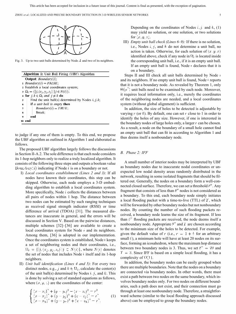
algorithm is motivated by the fact that a hole can always containan empty unit ball. Therefore, we can search for empty unit ballsin order to identify holes and boundary nodes.More specifically,a node can test if it is on a boundary by constructing a unit ballwith itself on the ball’s surface. If at least one such ball canbe found that no nodes are located inside, a hole is identified,and the node is a boundary node [see Node in Fig. 2(a) forexample].The above process is called unit ball fitting. It can be applied

to identify both inner and outer boundaries. However, it is ob-viously infeasible for a node to perform a complete test of unitball fitting via brute-force search because there are infinite pos-sible orientations to place the unit ball. Next, we will show thata localized algorithm with a polynomial computing complexitycan be employed to test if such an empty unit ball exists.Lemma 1: Node can construct an empty unit ball that

touches itself if and only if there exists an empty unit balltouching Node and two neighbors of Node (within ).

Proof: We first show the sufficient condition, which isstraightforward. If a unit ball touched by Node and twoneighbors of Node is empty, i.e., there is an empty unit ballwith Node and two neighbors of Node on its surface,Node has constructed such an empty unit ball touching itself.Consequently, a hole is identified and Node is a boundarynode.Now, we prove the necessary condition. If there exists an

empty unit ball with Node on its surface, we can always fixNode and rotate the ball until it touches another node within, denoted by Node [see Fig. 2(b)]. Note that if Node

does not exist, Node must be isolated, which conflicts withour assumption of well-connected networks (see Definition 3).Then, we can further rotate the ball with Line as an axis,

Fig. 2. Principles for UBF. (a) Empty unit ball touching Node . (b) Ballrotation.

until it touches another node, denoted by Node . Similarly,Node must exist because otherwise Line is degeneratedand thus against Definition 3. Therefore, if Node can con-struct an empty unit ball that touches itself, we can always findan empty unit ball with Node and two neighbors of Nodeon its surface.Based on the sufficient condition and the necessary condition

discussed above, the lemma is thus proven.According to Lemma 1, we can show that a node can deter-

mine if it can construct an empty unit ball that touches itself bya localized algorithm with a computing complexity of . Ifsuch an empty unit ball can be constructed, the node must be aboundary node. Formally, we have the following theorem.Theorem 1: Node can determine if it can construct an

empty unit ball that touches itself by testing unit ballsand nodes for each ball.

Proof: According to Lemma 1, Node can exhaustivelytest all unit balls determined byNode and its neighbors. GivenNode and any two neighbors (whose distances to Node areless than ), zero or one or two unit balls can be formed suchthat the three nodes are on the surface(s). Fig. 3 illustrates an ex-ample where two unit balls are determined by three nodes. SinceNode has about , or , neighboring nodes withinthe distance of , it needs to test up to unitballs. For each unit ball, about , or , nodes must betested to judge if it is empty. Therefore, the overall computingcomplexity is .3) Algorithm Description: Theorem 1 provides a clear guid-

ance for our algorithm development. It suggests a distributedand localized algorithm where each node tests unit balls



Fig. 3. Up to two unit balls determined by Node and two of its neighbors.

to judge if any one of them is empty. To this end, we proposethe UBF algorithm as outlined in Algorithm 1 and elaborated asfollows.The proposed UBF algorithm largely follows the discussions

in Section II-A.2. The sole difference is that each node considersits 1-hop neighbors only to realize a truly localized algorithm. Itconsists of the following three steps and outputs a boolean value

indicating if Node is on a boundary or not.I) Local coordinates establishment (Lines 2 and 3): If allnodes have known their coordinates, this step can beskipped. Otherwise, each node employs a 3-D embed-ding algorithm to establish a local coordinates system.More specifically, Node collects the distances betweenall pairs of nodes within 1 hop. The distance betweentwo nodes can be estimated by such ranging techniquesas received signal strength indicator (RSSI) or timedifference of arrival (TDOA) [31]. The measured dis-tances are inaccurate in general, and the errors will bediscussed in Section V. Based on the pairwise distances,multiple schemes [32]–[36] are available to create alocal coordinates system for Node and its neighbors.Among them, [36] is adopted in our implementation.Once the coordinates system is established, Node keepsa set of neighboring nodes and their coordinates, i.e.,

, where denotesthe set of nodes that includes Node itself and its 1-hopneighbors.

II) Unit ball identification (Lines 4 and 5): For every twodistinct nodes, e.g., and , calculate the center(s)of the unit ball(s) determined by Nodes , and . Thisis done by solving a set of standard equations as follows,where are the coordinates of the center:

(1)

Depending on the coordinates of Nodes and , (1)may yield no solution, or one solution, or two solutionsfor .

III) Empty unit ball check (Lines 6–9): If there is no solution,i.e., Nodes , and do not determine a unit ball, noaction is taken. Otherwise, for each solution ofidentified above, check if any node in is located insidethe corresponding unit ball, i.e., if it is an empty unit ball.If an empty unit ball is found, Node declares that it ison a boundary.

Steps II and III check all unit balls determined by Nodeand its neighbors. If no empty unit ball is found, Node reportsthat it is not a boundary node. As revealed by Theorem 1, only

unit balls need to be examined by each node. Moreover,it requires local information only, i.e., merely the coordinatesof the neighboring nodes are needed, and a local coordinatessystem (without global alignment) is sufficient.In addition, the size of holes to be detected is adjustable by

varying (or ). By default, one can set close to 1 in order toidentify the holes of any size. However, if one is interested inthe boundary nodes of large holes only, a larger can be chosen.As a result, a node on the boundary of a small hole cannot findan empty unit ball that can fit in according to Algorithm 1 andthus deems itself a nonboundary node.

B. Phase 2: IFF

A small number of interior nodes may be interpreted by UBFas boundary nodes due to inaccurate nodal coordinates or un-expected low nodal density areas randomly distributed in thenetwork, resulting in some isolated fragments that should be fil-tered out. Generally, the nodes on a boundary form a well-con-nected closed surface. Therefore, we can set a threshold . Anyfragment that consists of less than nodes is not considered asa boundary. To this end, each boundary node simply initiatesa local flooding packet with a time-to-live (TTL) of , whichwill be forwarded by other boundary nodes but not nonboundarynodes. By counting the number of such flooding packets re-ceived, a boundary node learns the size of its fragment. If lessthan flooding packets are received, the node deems itself anonboundary node. Appropriate and are chosen accordingto the minimum size of the holes to be detected. For example,given the default value of (i.e., for an arbitrarysmall ), a minimum hole will have at least 20 nodes on its sur-face, forming an icosahedron, where the maximum hop distancebetween two boundary nodes is 3. Thus, we set and

. Since IFF is based on a simple local flooding, it has acomplexity of .In addition, the boundary nodes can be easily grouped when

there are multiple boundaries. Note that the nodes on a boundaryare connected via boundary nodes. In other words, there mustexist a path between two nodes on the same boundary, which in-volves boundary nodes only. For two nodes on different bound-aries, such a path does not exist, and their connection must gothrough at least one nonboundary node. Therefore, a straightfor-ward scheme (similar to the local flooding approach discussedabove) can be employed to group the boundary nodes.



C. Summary of Boundary Node Identification

By following the two phases outlined above, a node deter-mines whether it is on a boundary based on local informationonly. Its performance depends on the accuracy of distancemeasurement. As will be discussed in Section V, our simula-tions demonstrate that the proposed algorithms are effective,able to identify almost all boundary nodes with low missingand mistaken rates, when the distance errors are moderate[as shown in Fig. 1(g)]. Under high measurement errors, themistaken and missing rates naturally increase. However, themistakenly identified boundary nodes are all close to the trueboundary, mostly within 1 or 2 hops [see Fig. 1(h)]. At thesame time, the missed boundary nodes are uniformly scattered.Over 95% of such missed boundary nodes can find at least onecorrectly identified boundary node within their 1-hop neigh-borhood [as illustrated in Fig. 1(i)]. Therefore, the identifiedboundary nodes well represent the network boundary shapes.The complexity of the algorithm is dominated by Phase 1,i.e., UBF. Therefore, the overall computing complexity forboundary node detection is . While the nodal densitymay vary arbitrarily in theory, it is often bounded by a smallconstant in practical sensor network settings, where the radiorange is chosen properly by individual nodes to maintain thedesired nodal degree. Numeric results of computing complexitywill be presented in Section V.

III. TRIANGULAR BOUNDARY SURFACE CONSTRUCTION

The boundary nodes identified so far are discrete. Theylargely depict the network boundaries. However, many applica-tions require not only discrete boundary nodes, but also closedboundary surfaces. Moreover, it is highly desirable that suchsurfaces are locally planarized 2-manifold in order to applyavailable 2-D graphic tools on 3-D surfaces.In this research, we implement an algorithm that constructs

locally planarized triangular meshes on the identified 3-Dboundaries. We adopt the method proposed in [30] that canproduce a 2-D planar subgraph (which, however, is not a trian-gular mesh) and extend it to 3-D surfaces to achieve completetriangulation without degenerated edges. The algorithm islocalized and based on connectivity only. It consists of thefollowing five steps.I) Landmark selection: The boundary nodes employ a dis-tributed algorithm (e.g., [37]) to elect a subset of nodesas “landmarks.” Any two landmarks must be hopsapart. determines the fineness of the mesh. It is usuallyset between 3–5 in our implementation. A nonlandmarkboundary node is associated with the closest landmark.If it has the same distance (in hop counts) to multiplelandmarks, it chooses the one with the smallest ID as atiebreaker. This step creates a set of approximate Voronoicells on each boundary [as shown in Fig. 1(c)].

II) Construction of Combinatorial Delaunay Graph (CDG):Each nonlandmark boundary node checks if it has aneighboring boundary node that is associated with adifferent landmark. If it has, a message is sent to bothlandmarks to indicate that they are neighboring land-marks. If we simply connect all neighboring landmarks,

we arrive at a CDG as illustrated in Fig. 1(d), which isthe respective dual of the Voronoi cells on a boundaryfound in Step I. However, such a CDG is not planar [seethe crossing edges highlighted in Fig. 1(d)].

III) Construction of Combinatorial Delaunay Map (CDM):Each landmark node decides whether it connects to aneighboring landmark as follows. It sends a packet to aneighboring landmark through the shortest path (based onthe identified boundary nodes only). The packet recordsthe nodes along the path. The two landmarks are said tobe connected if and only if the following two conditionsare satisfied. First, all nodes visited by the packet are as-sociated to these two landmarks only. Second, assume thepacket is sent from Landmark to Landmark . Then,the packet must visit the nodes associated with Land-mark first, and then followed by the nodes associatedwith Landmark , without interleaving. If the above twoconditions are satisfied, Landmark sends an ACK toLandmark , and a virtual edge is added between them.The boundary nodes that receive such ACK records thatthey are on the shortest path between two connected land-marks. This step yields a CDM. It is proven that CDM isa planar graph [30].

IV) Construction of triangular mesh: The CDM obtained sofar is planar, but not always a triangular mesh. Polygonswith more than three edges may exist [see the polygonhighlighted in Fig. 1(e)]. To achieve complete triangula-tion, appropriate edges should be added between someneighboring landmarks. If a landmark, e.g., Landmark ,has a nonconnected neighboring landmark (e.g., Land-mark ), it sends a connection packet to the latter (viathe shortest path based on the identified boundary nodes).The packet will be dropped if it reaches an intermediatenode that is already on the shortest path between two con-nected landmarks in order to avoid crossing edges. If theconnection packet arrives at Landmark , a virtual edgecan be safely added, and an ACK is sent back to Land-mark . Similarly, the boundary nodes that receive theACK records that they are on the shortest path betweentwo connected landmarks. This step adds all possible vir-tual edges to divide polygons into triangles.

V) Edge flip: To ensure themesh to be a 2-manifold, each vir-tual edge must be associated with two triangles. After theabove step, there still possibly exist edges [like Edgein Fig. 4(a)] with three triangular faces, formed with threecorresponding nodes (i.e., , and ). Such edges canbe detected by trivial local signaling. For each such edge,a transformation is done as follows. First, Edge isremoved. Second, two shortest edges are added betweenthe corresponding nodes, i.e., Nodes , and . Forexample, assume is longer than and . Then,two virtual edges and are added, resulting inFig. 4(b), where no edge has more than two faces. Notethat the polygon is not a face on the surface. Untilnow, we arrive at a planar triangular mesh for each 3-Dboundary surface, as illustrated in Fig. 1(f).

The above algorithm ensures to form a closed triangular meshsurface for each boundary. The established triangular mesh is a



Fig. 4. Illustration of edge flip. Edge has three faces before edge flip. It isremoved and replaced by Edges and . (a) Before edge flip. (b) Afteredge flip.

locally planarized 2-manifold, although the whole 3-D surfaceis not planar. A virtual edge on a mesh surface has exactly twotriangular faces. Such salient properties enable application ofmany useful graph theory tools on 3-D boundary surfaces, in-cluding embedding, localization, partition, and greedy routingamong many others.Note that since the triangular mesh is established based on

landmarks only, a small number of nodes (that are on or close tothe boundaries) may be located outside the mesh surfaces. Thenumber of such nodes is determined by and the curvature ofthe boundary. The larger the , the coarser the mesh surfaces,resulting in more nodes left outside. An appropriate can bechosen according to the needs of specific applications. For ex-ample, Fig. 1(f) shows the results with .In addition, we observed that the triangular mesh is not

seriously deformed under distance measurement errors. Asdiscussed in Section II-C, the mistakenly identified boundarynodes are close to the true boundary, and the missing boundarynodes are uniformly distributed. Therefore, the identifiedboundary nodes can still well represent the network boundaries,even under distance measurement errors. This is verified byour simulations. For example, Fig. 1(j)–(l) shows results under20%, 30%, and 40% distance measurement errors, respectively.Fig. 1(j)–(l) exhibits similar triangular mesh as Fig. 1(j), whichis free of distance measurement errors.

IV. BOUNDARY DETECTION IN DYNAMIC WIRELESS SENSORNETWORKS

In many application scenarios, the network topology changesover time due to environment dynamics (such as, water flow,wind, and animal movement) or the evolvement of the networkitself (as links break or nodes run out of batteries). Topologydynamics often cause the change of network boundary, callingfor an effective online boundary detection algorithm, with lowoverhead and high energy efficiency.In this section, we will introduce effective algorithms that not

only identify boundary nodes, but alsomaintain a closed trianglemesh surface in dynamic wireless sensor networks.

A. Online Boundary Nodes Detection

In this work, we consider a general random mobility model,where a node moves for a distance of that is (less than trans-mission range ) to any direction in a time unit. Note that wedo not consider any special radio model constraints here, except

Fig. 5. Example of the random mobility model. The node is highlighted bygreen crosses, when it moves to the boundary.

Fig. 6. Three layers of nodes in online boundary detection. Red nodes are theboundary nodes , blue nodes are the candidates nodes , and therest of the nodes with aqua color will not be involved in the UBF algorithm.

the maximum radio transmission range . The sensors’ mo-bility is constrained by their container (e.g., seabed and shore).Fig. 5 illustrates how a node moves according to the above mo-bility model. As can be seen, sometimes it moves to the surface,becoming a boundary node (highlighted as green crosses), andsometimes it moves inside.The UBF algorithm is localized only involving 1-hop

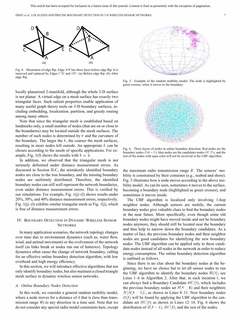
neighbor nodes. Although sensors are mobile, the currentboundary nodes give valuable clues to find the boundary nodesin the near future. More specifically, even though some oldboundary nodes might have moved inside and not be boundarynodes anymore, they should still be located near the boundaryand thus help to narrow down the boundary candidates. As amatter of fact, the previous boundary nodes and their neighbornodes are good candidates for identifying the new boundarynodes. The UBF algorithm can be applied only to these candi-date nodes instead of all nodes in the network in order to reduceenergy consumption. The online boundary detection algorithmis outlined as follows.Since there is no clue about the boundary nodes at the be-

ginning, we have no choice but to let all sensor nodes to runthe UBF algorithm to identify the boundary nodes ; seeLines 1–6 in Algorithm 2. After that, in each iteration , wecan always find a Boundary Candidate , which includesthe previous boundary nodes set and their neighbors

, as shown in Lines 8–11. New boundary nodeswill be found by applying the UBF algorithm to the can-

didate set as shown in Lines 12–16. Fig. 6 shows thedistribution of , and the rest of the nodes.



B. Online Triangle Mesh Updating

While we can simply reconstruct the triangle mesh basedon the newly identified boundary nodes, a more effective ap-proach is to maintain the triangle mesh constructed previouslyand update it according to the new boundary. We observe thatthe Voronoi cells are more stable than boundary nodes, and thetriangle mesh is only determined by the Voronoi cells, morespecifically the landmarks of the cells. How to update the land-marks forming the triangle mesh is the key to solve this problemefficiently.However, the selection of new landmark is not trivial be-

cause new triangle mesh must satisfy two properties. First, allof the landmarks must be boundary nodes. Second, there are nocrossing edges between landmarks. Some landmarks in the pre-vious round might not be boundary nodes in this round due tomobility, and thus are not eligible for new landmarks. Therefore,we have to find a new boundary node as a new landmark to re-place the old one, if the old landmark is not on the boundary anymore. Picking the boundary node closest to the old landmark isa straightforward way to fulfill the mission.It is much more challenging to preserve the second property,

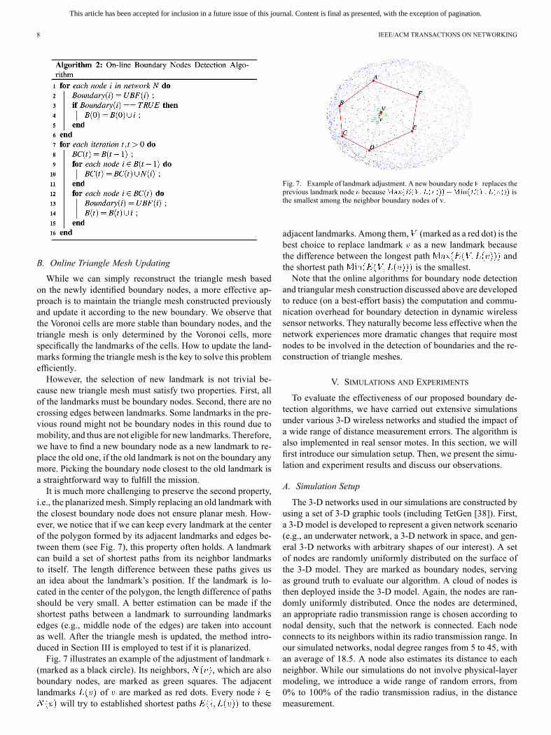
i.e., the planarizedmesh. Simply replacing an old landmark withthe closest boundary node does not ensure planar mesh. How-ever, we notice that if we can keep every landmark at the centerof the polygon formed by its adjacent landmarks and edges be-tween them (see Fig. 7), this property often holds. A landmarkcan build a set of shortest paths from its neighbor landmarksto itself. The length difference between these paths gives usan idea about the landmark’s position. If the landmark is lo-cated in the center of the polygon, the length difference of pathsshould be very small. A better estimation can be made if theshortest paths between a landmark to surrounding landmarksedges (e.g., middle node of the edges) are taken into accountas well. After the triangle mesh is updated, the method intro-duced in Section III is employed to test if it is planarized.Fig. 7 illustrates an example of the adjustment of landmark

(marked as a black circle). Its neighbors, , which are alsoboundary nodes, are marked as green squares. The adjacentlandmarks of are marked as red dots. Every node

will try to established shortest paths to these

Fig. 7. Example of landmark adjustment. A new boundary node replaces theprevious landmark node because isthe smallest among the neighbor boundary nodes of v.

adjacent landmarks. Among them, (marked as a red dot) is thebest choice to replace landmark as a new landmark becausethe difference between the longest path andthe shortest path is the smallest.Note that the online algorithms for boundary node detection

and triangular mesh construction discussed above are developedto reduce (on a best-effort basis) the computation and commu-nication overhead for boundary detection in dynamic wirelesssensor networks. They naturally become less effective when thenetwork experiences more dramatic changes that require mostnodes to be involved in the detection of boundaries and the re-construction of triangle meshes.

V. SIMULATIONS AND EXPERIMENTS

To evaluate the effectiveness of our proposed boundary de-tection algorithms, we have carried out extensive simulationsunder various 3-D wireless networks and studied the impact ofa wide range of distance measurement errors. The algorithm isalso implemented in real sensor motes. In this section, we willfirst introduce our simulation setup. Then, we present the simu-lation and experiment results and discuss our observations.

A. Simulation Setup

The 3-D networks used in our simulations are constructed byusing a set of 3-D graphic tools (including TetGen [38]). First,a 3-D model is developed to represent a given network scenario(e.g., an underwater network, a 3-D network in space, and gen-eral 3-D networks with arbitrary shapes of our interest). A setof nodes are randomly uniformly distributed on the surface ofthe 3-D model. They are marked as boundary nodes, servingas ground truth to evaluate our algorithm. A cloud of nodes isthen deployed inside the 3-D model. Again, the nodes are ran-domly uniformly distributed. Once the nodes are determined,an appropriate radio transmission range is chosen according tonodal density, such that the network is connected. Each nodeconnects to its neighbors within its radio transmission range. Inour simulated networks, nodal degree ranges from 5 to 45, withan average of 18.5. A node also estimates its distance to eachneighbor. While our simulations do not involve physical-layermodeling, we introduce a wide range of random errors, from0% to 100% of the radio transmission radius, in the distancemeasurement.



Fig. 8. Example of underwater network. (a) Network model. In contrast to Figs. 9(a), 10(a), 11(a), and 12(a), where the network model shows a set of wirelessnodes deployed, the network model in this figure gives the actual 3-D model for better visualization. (b) Boundary nodes. (c) Triangular mesh.

Fig. 9. Example of a 3-D space network with an internal hole. (a) Network model. (b) Boundary nodes. (c) Triangular mesh.

Fig. 10. Example of a 3-D space network with two internal holes. (a) Network model. (b) Boundary nodes. (c) Triangular mesh.

Fig. 11. Example of a 3-D network in a bended pipe. (a) Network model.(b) Boundary nodes. (c) Triangular mesh.

For each simulated network, the input includes a set of thenodes (both interior and boundary nodes), the local 1-hop con-nectivity of each node, and the distance measurement (with var-ious errors) within 1-hop neighborhood.

B. Simulation Results

We run our proposed distributed and localized algorithmsfor boundary node detection and surface construction. First,each node establishes a local coordinates system by using dis-tributed multidimensional scaling [36] based on local distancemeasurement. Then, boundary node identification is performed,followed by the triangular mesh algorithm.Several examples of our simulated networks are given in

Figs. 8–12. Figs. 8 illustrates an underwater network, wherenodes are distributed from the surface to the bottom of the

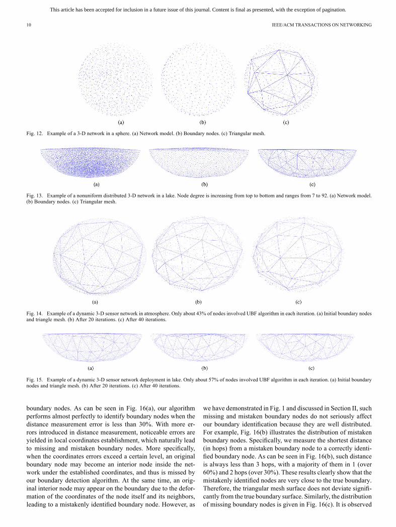
ocean. As shown in Fig. 8(b) and (c), our algorithms effectivelyidentify the boundaries of both smooth water surface and thebumpy bottom. Figs. 9 and 10 depict a 3-D network deployedin the space (e.g., for chemical dispersion sampling in 3-Dspace). They have one and two internal holes, respectively, dueto uncontrolled drift of sensor nodes. These examples demon-strate that our algorithm works for not only outer boundary, butalso the boundaries of interior holes. Figs. 11 and 12 show 3-Dnetworks deployed in a bended pipe and a sphere, respectively.Fig. 13 demonstrates a nonuniform distributed 3-D network.The node density is increasing from top to bottom, and nodedegree ranges from 7 up to 92. As can be seen, boundary nodesare accurately identified, and the triangular mesh surfaces arewell constructed in the all networks.We have also simulated nodal mobility and run the online

boundary detection and triangle mesh updating algorithms in-troduced in Section IV. Two examples are given in Figs. 14 and15. As can be seen, landmarks change overtime, but the trianglemesh remains nicely distributed. They clearly demonstrate thatthe online boundary detection algorithm and boundary mesh up-dating algorithm are adaptive to the dynamics of network. Only43% and 57% of nodes on average involve UBF in Figs. 14 and15, respectively. All the boundary nodes are successfully iden-tified. Larger-scale networks will benefit more from our algo-rithm because only nodes within one hop layer from the surfacerun the algorithms.Fig. 16 illustrates the performance statistics obtained from

our simulations. The results are based on over 10 000 sample



Fig. 12. Example of a 3-D network in a sphere. (a) Network model. (b) Boundary nodes. (c) Triangular mesh.

Fig. 13. Example of a nonuniform distributed 3-D network in a lake. Node degree is increasing from top to bottom and ranges from 7 to 92. (a) Network model.(b) Boundary nodes. (c) Triangular mesh.

Fig. 14. Example of a dynamic 3-D sensor network in atmosphere. Only about 43% of nodes involved UBF algorithm in each iteration. (a) Initial boundary nodesand triangle mesh. (b) After 20 iterations. (c) After 40 iterations.

Fig. 15. Example of a dynamic 3-D sensor network deployment in lake. Only about 57% of nodes involved UBF algorithm in each iteration. (a) Initial boundarynodes and triangle mesh. (b) After 20 iterations. (c) After 40 iterations.

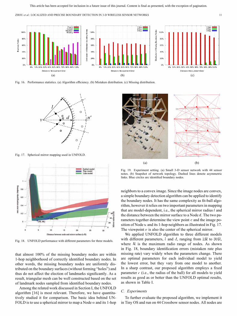
boundary nodes. As can be seen in Fig. 16(a), our algorithmperforms almost perfectly to identify boundary nodes when thedistance measurement error is less than 30%. With more er-rors introduced in distance measurement, noticeable errors areyielded in local coordinates establishment, which naturally leadto missing and mistaken boundary nodes. More specifically,when the coordinates errors exceed a certain level, an originalboundary node may become an interior node inside the net-work under the established coordinates, and thus is missed byour boundary detection algorithm. At the same time, an orig-inal interior node may appear on the boundary due to the defor-mation of the coordinates of the node itself and its neighbors,leading to a mistakenly identified boundary node. However, as

we have demonstrated in Fig. 1 and discussed in Section II, suchmissing and mistaken boundary nodes do not seriously affectour boundary identification because they are well distributed.For example, Fig. 16(b) illustrates the distribution of mistakenboundary nodes. Specifically, we measure the shortest distance(in hops) from a mistaken boundary node to a correctly identi-fied boundary node. As can be seen in Fig. 16(b), such distanceis always less than 3 hops, with a majority of them in 1 (over60%) and 2 hops (over 30%). These results clearly show that themistakenly identified nodes are very close to the true boundary.Therefore, the triangular mesh surface does not deviate signifi-cantly from the true boundary surface. Similarly, the distributionof missing boundary nodes is given in Fig. 16(c). It is observed



Fig. 16. Performance statistics. (a) Algorithm efficiency. (b) Mistaken distribution. (c) Missing distribution.

Fig. 17. Spherical mirror mapping used in UNFOLD.

Fig. 18. UNFOLD performance with different parameters for three models.

that almost 100% of the missing boundary nodes are within1-hop neighborhood of correctly identified boundary nodes. Inother words, the missing boundary nodes are uniformly dis-tributed on the boundary surfaces (without forming “holes”) andthus do not affect the election of landmarks significantly. As aresult, triangular mesh can be well constructed based on the setof landmark nodes sampled from identified boundary nodes.Among the related work discussed in Section I, the UNFOLD

algorithm [16] is most relevant. Therefore, we have quantita-tively studied it for comparison. The basic idea behind UN-FOLD is to use a spherical mirror to map a Node and its 1-hop

Fig. 19. Experiment setting. (a) Small 3-D sensor network with 44 sensornotes. (b) Snapshot of network topology. Dashed lines denote asymmetriclinks. Blue circles are identified boundary nodes.

neighbors to a convex image. Since the image nodes are convex,a simple boundary detection algorithm can be applied to identifythe boundary nodes. It has the same complexity as fit-ball algo-rithm, however it relies on two important parameters inmappingthat are model-dependent, i.e., the spherical mirror radius andthe distance between the mirror surface to a Node . The two pa-rameters together determine the view point and the image po-sition of Node and its 1-hop neighbors as illustrated in Fig. 17.The viewpoint is also the center of the spherical mirror.We applied UNFOLD algorithm to three different models

with different parameters, and , ranging from to ,where is the maximum radio range of nodes. As shownin Fig. 18, boundary identification errors (mistaken rate plusmissing rate) vary widely when the parameters change. Thereare optimal parameters for each individual model to yieldthe lowest error, but they vary from one model to another.In a sharp contrast, our proposed algorithm employs a fixedparameter (i.e., the radius of the ball) for all models to yieldresults as good as or better than the UNFOLD optimal results,as shown in Table I.

C. Experiments

To further evaluate the proposed algorithm, we implement itin Tiny OS and run on 44 Crossbow sensor nodes. All nodes are



Fig. 20. Asymmetric links problem and solution. (a) Asymmetric Link . (b) Limited broadcast. (c) Number of mistaken nodes comparison between with andwithout limited broadcasting.

TABLE IBOUNDARY IDENTIFICATION ERRORS COMPARISON

configured to use close to minimum radio transmission power(Level 2), with a communication range between 25–25 cm.They are tied onto a rack to form a small 3-D sensor networkshown in Fig. 19(a).Every sensor periodically broadcasts a beacon message with

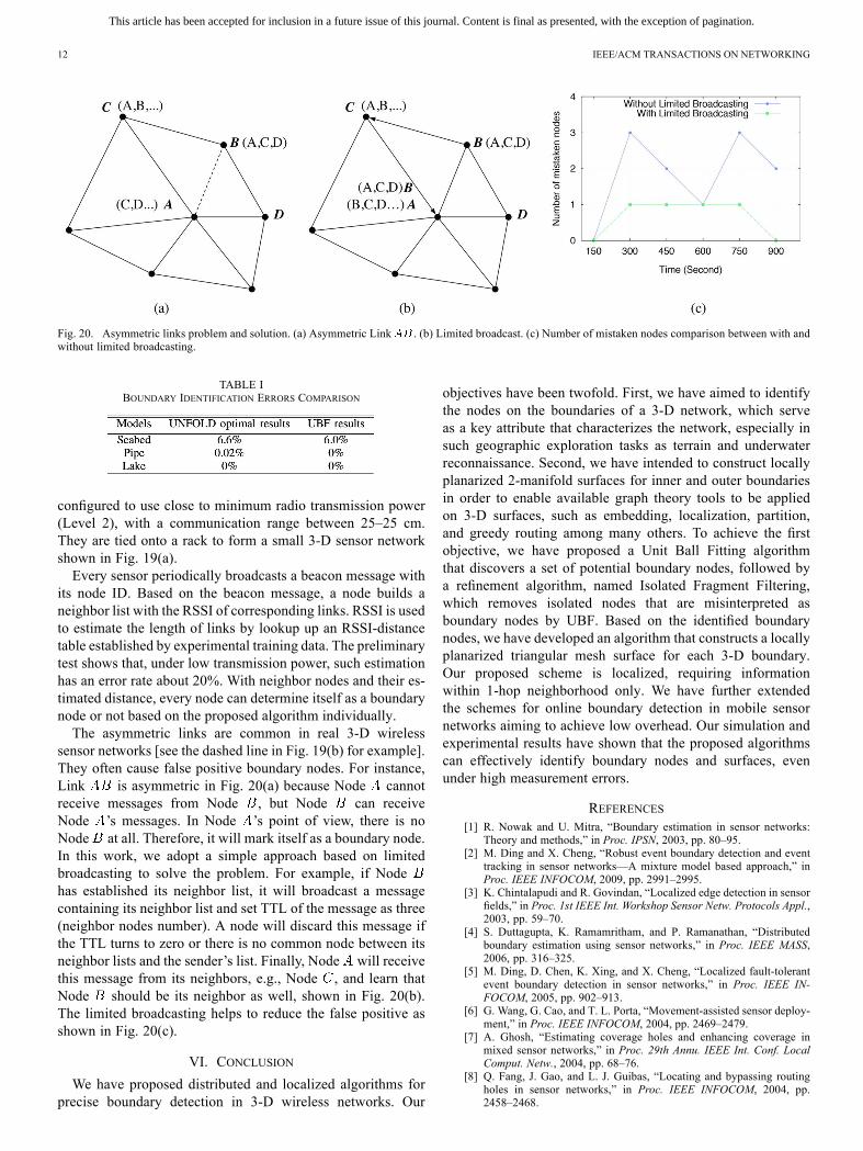
its node ID. Based on the beacon message, a node builds aneighbor list with the RSSI of corresponding links. RSSI is usedto estimate the length of links by lookup up an RSSI-distancetable established by experimental training data. The preliminarytest shows that, under low transmission power, such estimationhas an error rate about 20%. With neighbor nodes and their es-timated distance, every node can determine itself as a boundarynode or not based on the proposed algorithm individually.The asymmetric links are common in real 3-D wireless

sensor networks [see the dashed line in Fig. 19(b) for example].They often cause false positive boundary nodes. For instance,Link is asymmetric in Fig. 20(a) because Node cannotreceive messages from Node , but Node can receiveNode ’s messages. In Node ’s point of view, there is noNode at all. Therefore, it will mark itself as a boundary node.In this work, we adopt a simple approach based on limitedbroadcasting to solve the problem. For example, if Nodehas established its neighbor list, it will broadcast a messagecontaining its neighbor list and set TTL of the message as three(neighbor nodes number). A node will discard this message ifthe TTL turns to zero or there is no common node between itsneighbor lists and the sender’s list. Finally, Node will receivethis message from its neighbors, e.g., Node , and learn thatNode should be its neighbor as well, shown in Fig. 20(b).The limited broadcasting helps to reduce the false positive asshown in Fig. 20(c).

VI. CONCLUSION

We have proposed distributed and localized algorithms forprecise boundary detection in 3-D wireless networks. Our

objectives have been twofold. First, we have aimed to identifythe nodes on the boundaries of a 3-D network, which serveas a key attribute that characterizes the network, especially insuch geographic exploration tasks as terrain and underwaterreconnaissance. Second, we have intended to construct locallyplanarized 2-manifold surfaces for inner and outer boundariesin order to enable available graph theory tools to be appliedon 3-D surfaces, such as embedding, localization, partition,and greedy routing among many others. To achieve the firstobjective, we have proposed a Unit Ball Fitting algorithmthat discovers a set of potential boundary nodes, followed bya refinement algorithm, named Isolated Fragment Filtering,which removes isolated nodes that are misinterpreted asboundary nodes by UBF. Based on the identified boundarynodes, we have developed an algorithm that constructs a locallyplanarized triangular mesh surface for each 3-D boundary.Our proposed scheme is localized, requiring informationwithin 1-hop neighborhood only. We have further extendedthe schemes for online boundary detection in mobile sensornetworks aiming to achieve low overhead. Our simulation andexperimental results have shown that the proposed algorithmscan effectively identify boundary nodes and surfaces, evenunder high measurement errors.

REFERENCES[1] R. Nowak and U. Mitra, “Boundary estimation in sensor networks:

Theory and methods,” in Proc. IPSN, 2003, pp. 80–95.[2] M. Ding and X. Cheng, “Robust event boundary detection and event

tracking in sensor networks—A mixture model based approach,” inProc. IEEE INFOCOM, 2009, pp. 2991–2995.

[3] K. Chintalapudi and R. Govindan, “Localized edge detection in sensorfields,” in Proc. 1st IEEE Int. Workshop Sensor Netw. Protocols Appl.,2003, pp. 59–70.

[4] S. Duttagupta, K. Ramamritham, and P. Ramanathan, “Distributedboundary estimation using sensor networks,” in Proc. IEEE MASS,2006, pp. 316–325.

[5] M. Ding, D. Chen, K. Xing, and X. Cheng, “Localized fault-tolerantevent boundary detection in sensor networks,” in Proc. IEEE IN-FOCOM, 2005, pp. 902–913.

[6] G. Wang, G. Cao, and T. L. Porta, “Movement-assisted sensor deploy-ment,” in Proc. IEEE INFOCOM, 2004, pp. 2469–2479.

[7] A. Ghosh, “Estimating coverage holes and enhancing coverage inmixed sensor networks,” in Proc. 29th Annu. IEEE Int. Conf. LocalComput. Netw., 2004, pp. 68–76.

[8] Q. Fang, J. Gao, and L. J. Guibas, “Locating and bypassing routingholes in sensor networks,” in Proc. IEEE INFOCOM, 2004, pp.2458–2468.



[9] C. Zhang, Y. Zhang, and Y. Fang, “Localized algorithms for coverageboundary detection in wireless sensor networks,” Wireless Netw., vol.15, no. 1, pp. 3–20, 2009.

[10] R. Ghrist and A. Muhammad, “Coverage and hole-detection in sensornetworks via homology,” in Proc. IPSN, 2005, pp. 254–260.

[11] S. Funke, “Topological hole detection in wireless sensor networks andits applications,” in Proc. DIALM-POMC, 2005, pp. 44–53.

[12] A. Kroller, S. P. Fekete, D. Pfisterer, and S. Fischer, “Deterministicboundary recognition and topology extraction for large sensor net-works,” in Proc. ACM-SIAM SODA, 2006, pp. 1000–1009.

[13] Y. Wang, J. Gao, and J. S. B. Mitchell, “Boundary recognition insensor networks by topological methods,” in Proc. ACM/IEEE Mo-biCom, 2006, pp. 122–133.

[14] W. Cheng et al., “Underwater localization in sparse 3D acoustic sensornetworks,” in Proc. IEEE INFOCOM, 2008, pp. 798–806.

[15] H. Zhou, S. Xia, M. Jin, and H. Wu, “Localized algorithm for preciseboundary detection in 3D wireless networks,” in Proc. ICDCS, 2010,pp. 744–753.

[16] F. Li, J. Luo, C. Zhang, S. Xin, and Y. He, “UNFOLD: Uniform faston-line boundary detection for dynamic 3D wireless sensor networks,”in Proc. MobiHoc, 2011, pp. 141–152.

[17] H. Jiang, S. Zhang, G. Tan, and C.Wang, “CABET: Connectivity-basedboundary extraction of large-scale 3D sensor networks,” in Proc. IEEEINFOCOM, 2011, pp. 784–792.

[18] H. Zhou, H. Wu, and M. Jin, “A robust boundary detection algorithmbased on connectivity only for 3D wireless sensor networks,” in Proc.IEEE INFOCOM, 2012, pp. 1602–1610.

[19] C. Liu and J. Wu, “Efficient geometric routing in three dimensional adhoc networks,” in Proc. IEEE INFOCOM, 2009, pp. 2751–2755.

[20] T. F. G. Kao and J. Opatmy, “Position-based routing on 3D geometricgraphs in mobile ad hoc networks,” in Proc. 17th Can. Conf. Comput.Geometry, 2005, pp. 88–91.

[21] J. Opatrny, A. Abdallah, and T. Fevens, “Randomized 3D position-based routing algorithms for Ad-hoc networks,” in Proc. 3rd Annu. Int.Conf. Mobile Ubiquitous Syst., Netw. Services, 2006, pp. 1–8.

[22] R. Flury and R. Wattenhofer, “Randomized 3D geographic routing,” inProc. IEEE INFOCOM, 2008, pp. 834–842.

[23] F. Li, S. Chen, Y. Wang, and J. Chen, “Load balancing routing inthree dimensional wireless networks,” in Proc. IEEE ICC, 2008, pp.3073–3077.

[24] D. Pompili, T. Melodia, and I. F. Akyildiz, “Routing algorithms fordelay-insensitive and delay-sensitive applications in underwater sensornetworks,” in Proc. ACM/IEEE MobiCom, 2006, pp. 298–309.

[25] X. Cheng, A. Thaeler, G. Xue, and D. Chen, “TPS: A time-based posi-tioning scheme for outdoor wireless sensor networks,” in Proc. IEEEINFOCOM, 2004, vol. 4, pp. 2685–2696.

[26] X. Bai, C. Zhang, D. Xuan, J. Teng, andW. Jia, “Low-connectivity andfull-coverage three dimensional networks,” in Proc. ACM MobiHoc,2009, pp. 145–154.

[27] X. Bai, C. Zhang, D. Xuan, and W. Jia, “Full-coverage and K-connec-tivity three dimensional networks,” in Proc. IEEE IN-FOCOM, 2009, pp. 388–396.

[28] J. Allred et al., “SensorFlock: An airborne wireless sensor network ofmicro-air vehicles,” in Proc. SenSys, 2007, pp. 117–129.

[29] J.-H. Cui, J. Kong, M. Gerla, and S. Zhou, “The challenges of buildingmobile underwater wireless networks for aquatic applications,” IEEENetw., vol. 20, no. 3, pp. 12–18, May–Jun. 2006.

[30] S. Funke and N. Milosavljevi, “How much geometry hides in connec-tivity?—Part II,” in Proc. ACM-SIAM SODA, 2007, pp. 958–967.

[31] Z. Zhong and T. He, “MSP: Multi-sequence positioning of wirelesssensor nodes,” in Proc. SenSys, 2007, pp. 15–28.

[32] H. Wu, C. Wang, and N.-F. Tzeng, “Novel self-configurable posi-tioning technique for multi-hop wireless networks,” IEEE/ACM Trans.Netw., vol. 13, no. 3, pp. 609–621, Jun. 2005.

[33] G. Giorgetti, S. Gupta, and G.Manes, “Wireless localization using self-organizing maps,” in Proc. IPSN, 2007, pp. 293–302.

[34] L. Li and T. Kunz, “Localization applying an efficient neural networkmapping,” in Proc. 1st Int. Conf. Auton. Comput. Commun. Syst., 2007,pp. 1–9.

[35] Y. Shang, W. Ruml, Y. Zhang, and M. P. J. Fromherz, “Localizationfrom mere connectivity,” in Proc. ACM MobiHoc, 2003, pp. 201–212.

[36] Y. Shang and W. Ruml, “Improved MDS-based localization,” in Proc.IEEE INFOCOM, 2004, pp. 2640–2651.

[37] Q. Fang, J. Gao, L. J. Guibas, V. Silva, and L. Zhang, “GLIDER: Gra-dient landmark-based distributed routing for sensor networks,” inProc.IEEE INFOCOM, 2005, pp. 339–350.

[38] Fraunhofer-Institut FOKUS, Berlin, Germany, “berliOS,” [Online].Available: http://tetgen.berlios.de/

Hongyu Zhou (S’10) received the B.S. and M.S. de-grees from Sichuan University, Chengdu, China, in2006 and 2009, respectively, and the Ph.D. degree incomputer science from the University of Louisiana atLafayette, Lafayette, LA, USA, in 2013, all in com-puter science.He is working with Epic, Madison, WI, USA.

Su Xia (S’12–M’13) received the B.S. and M.S.degrees in radio engineering and computer sciencefrom Southeast University, Nanjing, China, in 1998and 2001, respectively, and the Ph.D. degree incomputer science from the University of Louisianaat Lafayette, Lafayette, LA, USA, in 2012.He is currently working with the Internet of

Things (IoT) Group, Cisco Systems, Inc., San Jose,CA, USA.

Miao Jin received the B.S. degree from BeijingUniversity of Posts and Telecommunications, Bei-jing, China, in 2000, and the M.S. and Ph.D. degreesfrom the State University of New York at StonyBrook, Stony Brook, NY, USA, in 2006 and 2008,respectively, all in computer science.She is an Associate Professor with the Center

for Advanced Computer Studies, University ofLouisiana at Lafayette, Lafayette, LA, USA. Herresearch results have been used as cover imagesof mathematics books and licensed by the Siemens

Healthcare Sector of Germany for virtual colonoscopy. Her research interestsare computational geometric and topological algorithms with applicationsin wireless sensor networks, computer graphics, computer vision, geometricmodeling, and medical imaging.Prof. Jin received the NSF CAREER Award in 2011.

Hongyi Wu (M’02) received the B.S. degree inscientific instruments from Zhejiang University,Hangzhou, China, in 1996, and the M.S. degree inelectrical engineering and Ph.D. degree in computerscience from the State University of New York(SUNY) at Buffalo, Buffalo, NY, USA, in 2000 and2002, respectively.Since then, he has been with the Center for

Advanced Computer Studies (CACS), Universityof Louisiana at Lafayette (UL Lafayette), Lafayette,LA, USA, where he is now a Professor and holds the

Alfred and Helen Lamson Endowed Professorship in Computer Science. Hisresearch spans delay-tolerant networks, radio frequency identification (RFID)systems, wireless sensor networks, and integrated heterogeneous wirelesssystems.Prof. Wu received the NSF CAREER Award in 2004 and the UL Lafayette

Distinguished Professor Award in 2011.

Documents

Localized and Precise Boundary Detection in 3-D Wireless Sensor Networks