Publications

11-20-2017

Localization of Interacting Fields in Five-Dimensional Braneworld Localization of Interacting Fields in Five-Dimensional Braneworld

Models Models

Dewi Wulandari Institut Teknologi Bandung

Triyanta Institut Teknologi Bandung

Jusak S. Kosasih Institut of Teknologi Bandung

Douglas Singleton California State University, Fresno

Preston Jones Embry-Riddle Aeronautical University, jonesp13@erau.edu

Follow this and additional works at: https://commons.erau.edu/publication

Part of the Physics Commons

Scholarly Commons Citation Scholarly Commons Citation Wulandari, D., Triyanta, Kosasih, J. S., Singleton, D., & Jones, P. (2017). Localization of Interacting Fields in Five-Dimensional Braneworld Models. International Journal of Modern Physics A, 32(32). https://doi.org/10.1142/S0217751X17501913

This Article is brought to you for free and open access by Scholarly Commons. It has been accepted for inclusion in Publications by an authorized administrator of Scholarly Commons. For more information, please contact commons@erau.edu.

brought to you by COREView metadata, citation and similar papers at core.ac.uk

provided by Embry-Riddle Aeronautical University

Localization of Interacting Fields in Five-Dimensional Braneworld

Models

Dewi Wulandari,1, ∗ Triyanta,2, † Jusak S. Kosasih,2, ‡

Douglas Singleton,3, § and Preston Jones4, ¶

1Physics Department, Universitas Negeri Medan, Medan Estate 20221, Indonesia

and

Department of Physics, Faculty of Mathematics and Natural Sciences,

Institut Teknologi Bandung, Jalan Ganesha 10 Bandung 40132, Indonesia

2Department of Physics, Faculty of Mathematics and Natural Sciences,

Institut Teknologi Bandung, Jalan Ganesha 10 Bandung 40132, Indonesia

3California State University Fresno, Fresno, CA 93740

4Embry Riddle Aeronautical University, Prescott, AZ 86301

1

Abstract

We study localization properties of fundamental fields which are coupled to one another through

the gauge mechanism both in the original Randall-Sundrum (RS) and in the modified Randall-

Sundrum (MRS) braneworld models: scalar-vector, vector-vector, and spinor-vector configuration

systems. For this purpose we derive conditions of localization, namely the finiteness of integrals

over the extra coordinate in the action of the system considered. We also derive field equations

for each of the systems and then obtain their solutions corresponding to the extra dimension by a

separation of variable method for every field involved in each system. We then insert the obtained

solutions into the conditions of localization to seek whether or not the solutions are in accordance

with the conditions of localization. We obtain that not all of the configuration systems considered

are localizable on the brane of the original RS model while, on the contrary, they are localizable

on the MRS braneworld model with some restrictions. In terms of field localizability on the brane,

this result shows that the MRS model is much better than the original RS model.

∗wulandaridewi@unimed.ac.id†triyanta@fi.itb.ac.id‡jusak@fi.itb.ac.id§dougs@mail.fresnostate.edu¶Preston.Jones1@erau.edu

2

I. INTRODUCTION

Extra dimensions were introduced in Kaluza-Klein models in order to unify electromag-

netic and gravitational forces. The extra dimension is of the order of the Planck length

so that direct experimental probing on it is hopeless [1]. Later on, extra dimensions were

proposed to address several issues such as cosmological constant, dark matter, non-locality,

and hierarchy problems [2–9]. Here, matter fields and gauge interactions are assumed to

be trapped in 4-dimensional sub-manifolds [5–7, 10] commonly referred to as brane world

models. The birth of braneworld models is also inspired by string theory [11, 12], a theory

that was built to unify all interactions including gravity.

The requirement of matter localization on the brane introduces various attempts to trap

matter. An example is shown in Refs. [13–15] that zero modes of all kinds of matter fields

and four-gravity may be localized on the (1+3)-dimensional brane in a six-dimensional bulk

by introducing an increasing and transverse gravitational potential. Other mechanisms to

address this issue in 6D are given in Refs. [16–18] and for higher dimensional brane world

models in Refs. [19–21].

The RS model [22] which is characterized by a metric of the form

ds2[y] = a2(x5)ηµνdxµdxν − dx5dx5, (1)

with a(x5) = e−k|x5|, x5 = y is the fifth coordinate, k is a constant and ηµν is the Minkowski

metric with signature (1,−1,−1,−1), is an appealing model as it resolves the hierarchy

problem [22]. However, this model is not a perfect braneworld model as not all types of

fundamental matter fields are localized on 3+1 brane in a simple manner [4, 23]. In fact,

only massless spin-0 fields are localized on the brane for decreasing warp factors [24]. For

increasing warp factors, on the other hand, only spin-1/2 fields are localized on the brane

[24]. Spin-1 fields are not localized for either a decreasing or an increasing warp factor [25].

This fact led authors in Ref. [26] to introduce the MRS model, specified by the metric

ds2[r] = a2(x5)ηµνdxµdxν − b2(x5)dx5dx5, b = a. (2)

We use r-coordinate instead of y-coordinate to indicate the fifth coordinate in the MRS

model. The localization properties for the MRS model are better as compared to the RS

model [26, 27]. This paper extends the work in Refs. [26, 27] by considering interacting

3

fields, fundamental fields that interact with vector fields through a gauge mechanism in

five-dimensional curved RS and MRS spacetimes, in addition to interacting with gravity. In

Section 3 we will look at the localization of interacting fields both in the RS and in the MRS

models. Conclusions are given in Section 4. However, before proceeding, we first make some

comments on Ref. [26] regarding the localization of spin-0 and spin-1/2 fields in the MRS

model.

II. COMMENTS ON REF. [26]

The action of massless scalar fields that only interact with gravity in a five-dimensional

modified RS model is given by:

S =

∫d5x√g∂MΦ∗∂MΦ, (3)

where g is the determinant of the MRS metric and the capital Latin indices M = 0, 1, 2, 3, 5.

Decomposing Φ(xM) = ϕ(xµ)χ(x5) the action becomes:

S =

∫ ∞0

dr√gχ∗χgµν

∫d4x∂µϕ

∗∂νϕ+

∫ ∞0

dr√ggrr∂rχ

∗∂rχ

∫d4xϕ∗ϕ. (4)

The fields are said to be localized on the brane if the action integrals over the extra dimension

from 0 to ∞ are finite. It means that the conditions for localization are∫ ∞0

dr√gχ∗χgµν =

∫ ∞0

dra2bχ∗χηµν = Nηµν , (5a)

∫ ∞0

dr√ggrr∂rχ

∗∂rχ = −∫ ∞0

dra4

b∂rχ

∗∂rχ = −m2. (5b)

In the last equation of eq. (30) in Ref. [26],√ggrr is written as −a2/b which equals −a in

the MRS model since in this model, b = a. However this is incorrect because√g = a4b,

grr = −1/b2 giving√ggrr = −a4/b which is equivalent to −a3 in the MRS model. The

general conclusion is still correct that massless scalar fields are localizable on the brane for

a decreasing warp factor while the massive ones are localizable both for a decreasing and an

increasing warp factors.

Now we go to the case of spinor fields Ψ in the five-dimensional MRS brane model. Ref.

[26] concludes that the spinor field is not localizable on the brane for both the decreasing and

increasing warp factors. This result is based on the definition of adjoint of spinor fields that

4

Ψ = Ψ+γ0 where γ0 is the zeroth Dirac matric in four-dimensional Minkowski spacetime.

However, if we define Ψ = Ψ+Γ0 where Γ0 is the zeroth Dirac matric in the five-dimensional

MRS curved spacetime the spinor field becomes localizable. The later definition of adjoint

more makes sense since both Ψ and Γ0 are defined in five-dimensional curved spacetime. To

prove the statement let us consider the following action

S =

∫d5x√g[ΨiΓMDMΨ], (6)

where g is the determinant of the metric (2), ΓM = eMMγM are gamma matrices in a curved

spacetime, γM are the gamma matrices in Minkowski spacetime with γ5 = iγ0γ1γ2γ3 while

eMM and eMM

are funfbeins and their inverses, respectively, and Ψ = Ψ+Γ0 = (Ψ∗)T e00γ0. DM

are the covariant derivatives defined in Ref. [26].

Decomposing the spinor Ψ(xM) in a five dimensional spacetime as

Ψ(xµ, r) =

ψ

(1)R (xµ)P

(1)R (r)

ψ(2)R (xµ)P

(2)R (r)

ψ(1)L (xµ)P

(1)L (r)

ψ(2)L (xµ)P

(2)L (r)

, (7)

the action (6) becomes,

S =

∫d5x

√g

a2(r)[ψ

(1)∗R P

(1)∗R (i∂0ψ

(1)R )P

(1)R + ψ

(2)∗R P

(2)∗R (i∂0ψ

(2)R )P

(2)R

+ψ(1)∗L P

(1)∗L (i∂0ψ

(1)L )P

(1)L + ψ

(2)∗L P

(2)∗L (i∂0ψ

(2)L )P

(2)L ]

+

∫d5x

√g

a2(r)[ψ

(2)∗R P

(2)∗R (i∂1ψ

(1)R )P

(1)R + ψ

(1)∗R P

(1)∗R (i∂1ψ

(2)R )P

(2)R

−ψ(2)∗L P

(2)∗L (i∂1ψ

(1)L )P

(1)L − ψ

(1)∗L P

(1)∗L (i∂1ψ

(2)L )P

(2)L ]

+

∫d5x

√g

a2(r)i[ψ

(2)∗R P

(2)∗R (i∂2ψ

(1)R )P

(1)R − ψ

(1)∗R P

(1)∗R (i∂2ψ

(2)R )P

(2)R

−ψ(2)∗L P

(2)∗L (i∂2ψ

(1)L )P

(1)L + ψ

(1)∗L P

(1)∗L (i∂2ψ

(2)L )P

(2)L ]

+

∫d5x

√g

a2(r)[ψ

(1)∗R P

(1)∗R (i∂3ψ

(1)R )P

(1)R − ψ

(2)∗R P

(2)∗R (i∂3ψ

(2)R )P

(2)R

−ψ(1)∗L P

(1)∗L (i∂3ψ

(1)L )P

(1)L + ψ

(2)∗L P

(2)∗L (i∂3ψ

(2)L )P

(2)L ]

−2k

∫d5x

√g

a2(r)[ψ

(1)∗L P

(1)∗L ψ

(1)R P

(1)R + ψ

(2)∗L P

(2)∗L ψ

(2)R P

(2)R

−ψ(1)∗R P

(1)∗R ψ

(1)L P

(1)L − ψ

(2)∗R P

(2)∗R ψ

(2)L P

(2)L ]

+

∫d5x

√g

a2(r)[ψ

(1)∗L P

(1)∗L ψ

(1)R ∂rP

(1)R + ψ

(2)∗L P

(2)∗L ψ

(2)R ∂rP

(2)R

−ψ(1)∗R P

(1)∗R ψ

(1)L ∂rP

(1)L − ψ

(2)∗R P

(2)∗R ψ

(2)L ∂rP

(2)L ]. (8)

5

We may choose the set of the localization conditions as the following (i = 1, 2)∫ ∞0

dra3(r)P(i)∗L P

(i)L =

∫ ∞0

dra3(r)P(i)∗R P

(i)R = 1; (9a)∫ ∞

0

dra3(r)P(1)∗L P

(2)L =

∫ ∞0

dra3(r)P(2)∗L P

(1)L

=

∫ ∞0

dra3(r)P(1)∗R P

(2)R =

∫ ∞0

dra3(r)P(2)∗R P

(1)R = 1; (9b)

−2k

∫ ∞0

dra3(r)P(i)∗L (r)P

(i)R (r) +

∫ ∞0

dra3(r)P(i)∗L (r)∂rP

(i)R (r) = −M ; (9c)

2k

∫ ∞0

dra3(r)P(i)∗R (r)P

(i)L (r)−

∫ ∞0

dra3(r)P(i)∗R (r)∂rP

(i)L (r) = −M. (9d)

Note that (9a) and (9b) give P(1)L = P

(2)L and P

(1)R = P

(2)R .

The Euler-Lagrange equation corresponding to the eq. (6), the covariant derivative in

Ref. [26], the Dirac equation iγµ∂µψ(x) = mψ(x) in the 4D Minkowski spacetime give the

equation for PR,L:

mP(i)R − 2kP

(i)R + ∂rP

(i)R = 0, (10a)

mP(i)L + 2kP

(i)L − ∂rP

(i)L = 0. (10b)

with their solutions

P(1)R = P

(2)R = b1/2e

r(−m+2k), (11a)

P(1)L = P

(2)L = d1/2e

r(m+2k). (11b)

where b1/2 and d1/2 are integration constants. Inserting these solutions to the localization

conditions (9a)-(9b) for right and left handed spinors respectively we get

|b1/2|2 = 2m− k, k < 2m, (12a)

|d1/2|2 = 2m+ k, k < −2m, (12b)

while equations (11a)-(11b) require k < 0 for finite values of the constants M . Intersecting

the above conditions gives k < 0 where m can be zero or positive. Thus one concludes that

both the right- and left-handed are localizable for increasing warp factor k < 0.

III. LOCALIZATION OF INTERACTING FIELDS

References [26, 27] reported the investigation of localization properties of fundamental

matter fields of various spins (spin-0, spin-1/2, and spin-1) that do not interact with other

6

fields except with gravity. Their interactions with gravity are introduced through the back-

ground RS and MRS metrics. In reality, most matter fields interact with other fields, in

addition to interaction with gravity, where the interaction is defined through a gauge mech-

anism. Examples such interacting fields are scalar field-photon coupling, spinor field-photon

coupling and interaction among spin-1 gluon (vector) fields, as described by the Yang-Mills

theory. Accordingly, it is necessary to expand the investigation in Refs. [26, 27] on field

localization by considering the following systems of interacting fields: scalar-vector, spinor-

vector, and vector-vector fields. We derive general localization conditions for each system

and check whether the conditions are satisfied by solutions of field equations corresponding

to extra dimension. Here we get the result that each considered system is not localizable in

the RS model. On the contrary all systems are localizable in the MRS model.

A. Scalar-Vector Fields

We first investigate the localization properties of a system of massless scalar and vector

fields coupled through a gauge mechanism. The system is described by the action:

S =

∫d5x√g

[(∂M − ieAM)Φ∗(∂M + ieAM)Φ− 1

4FMRF

MR

], (13)

where g is the determinant of the metric on which is dealing with i.e. the RS or MRS model,

FMR = ∂MAR − ∂RAM is the five-dimensional Faraday tensor with the five-dimensional

gauge vector field AM .

The corresponding field equations are

∂M(√ggMN∂NΦ) + ie∂M(

√ggMNANΦ) + ie

√ggMN∂NΦAM

−e2√ggMNAMANΦ = 0, (14)

∂P (√gF PM) + ie

√gΦ∂MΦ∗ − ie√gΦ∗∂MΦ− 2e2

√gAMΦ∗Φ = 0. (15)

Decomposing AM = (Aµ(xM), A5) = (aµ(xµ)c(y), Ay) and Φ(xM) = ϕ(xµ)χ(x5) and

7

taking A5 = Ay = const as in Ref. [26], the action becomes

S =

∫ ∞0

dx5√gχ∗χgµν

∫d4x∂µϕ

∗∂νϕ+

∫ ∞0

dx5√gg55∂5χ

∗∂5χ

∫d4xϕ∗ϕ

+

∫ ∞0

dx5√gc(x5)χ∗χgµν

∫d4xie∂µϕ

∗aνϕ

+

∫ ∞0

dx5√gg55∂5χ

∗A5χ

∫d4xieϕ∗ϕ

+

∫ ∞0

dx5√gc(x5)χ∗χgµν

∫d4x(−ie)∂νϕaµϕ∗

+

∫ ∞0

dx5√gg55χ∗∂5χA5

∫d4x(−ie)ϕϕ∗

+

∫ ∞0

dx5√gc2(x5)χ∗χgµν

∫d4xe2aµaνϕ

∗ϕ

+

∫ ∞0

dx5√gg55χ∗χA5A5

∫d4xe2ϕ∗ϕ

+

∫ ∞0

dx5√gc2(x5)gµνgαβ(−1

4)

∫d4xfµαfνβ

+2

∫ ∞0

dx5√g(∂5c(x

5))2gµνg55(−1

4)

∫d4xaµ(xν)aν(x

ν), (16)

giving the localization conditions for the fields: ∫ ∞0

dx5√gχ∗χgµν = N1η

µν ;∫ ∞0

dx5c(x5)√gχ∗χgµν = N2η

µν ;

∫ ∞0

dx5c2(x5)√gχ∗χgµν = N3η

µν ,

(17a)

∫ ∞0

dx5√gg55[(∂5χ

∗)(∂5χ) + ie(∂5χ∗)A5χ]

+

∫ ∞0

dx5√gg55[(−ie)χ∗∂5χA5 + e2χ∗χA5

2] = −mϕ2, (17b)∫ ∞

0

dx5√gc2gµνgαβ = N4η

µνηαβ;

∫ ∞0

dx5√g(∂5c)

2gµνg55 = ηµνmA2. (17c)

In the above, ϕ and aµ represent scalar and vector fields on the brane with their masses are

mϕ and mA respectively.

The field equations on the other hand, can be written as

1

χ∂5(√gg55∂5χ) + ie

1

χ∂5(√gg55A5χ) + ie

1

χ

√gg55A5∂5χ− e2

√gg55A5A5

=√ggµν(− 1

ϕ∂µ∂νϕ− iec

1

ϕ∂µ(aνϕ)− iec 1

ϕaµ∂νϕ+ e2c2aµaν), (18)

8

0 = c(x5)∂µ(√ggµνgMαfνα)− ∂µ(

√ggµνgM5aν(x

µ)∂5c(x5)

+∂5(√gg55gMαaα(xµ)∂5c(x

5))

+√ggMαχ∗χ[ieϕ∂αϕ

∗ − ieϕ∗∂αϕ+ 2e2c(x5)aα(xµ)ϕ∗ϕ]

+√ggM5[ieϕ∗ϕχ∂5χ

∗ − ieϕ∗ϕχ∗∂5χ+ 2e2A5χ∗χϕ∗ϕ]. (19)

The fulfillment of the fields on the localization conditions depends on the functions c(x5)

and χ(x5), the extra-dimension part solution of the field equations. The function c(x5)

can be deduced from the first field equation (18). The LHS of this equation depends only

on the extra coordinate x5 while the RHS depends on all coordinates where all non-extra

coordinates are fully inside the bracket. The dependence of all terms in the bracket on the

extra coordinate is given by the functions c(x5) and c2(x5). Thus considering all coordinates

are independent one another the function c(x5) should be a constant. Another possibility is

that the scalar ϕ and vector aν field functions should be such that the non-extra coordinates

disappear in the equation. For example, ϕ is an exponential function and aν is a constant.

However this is just a special case for ϕ and aν and we do not take this choice into account.

For c(x5)=const and take the constant equals unity the field equation for the vector field

simplifies into

0 =√ggµνgMα∂µfνα +

√ggMαχ∗χ[ieϕ∂αϕ

∗ − ieϕ∗∂αϕ+ 2e2aα(xµ)ϕ∗ϕ]

+√ggM5[ieϕ∗ϕχ∂5χ

∗ − ieϕ∗ϕχ∗∂5χ+ 2e2A5χ∗χϕ∗ϕ]. (20)

For M = β = 0, 1, 2, 3 and M = 5 respectively we have

∂µfµβ + a2(y)χ∗χ[ieϕ∂βϕ∗ − ieϕ∗∂βϕ+ 2e2aβϕ∗ϕ] = 0, (21a)

ie(∂5χ∗)χ− ieχ∗(∂5χ) + 2e2A5χ

∗χ = 0. (21b)

Until now, all we have discussed is general. It applies to any models. It is time now

to look at the RS model characterized by√g = a4(y), gµν = a−2(y)ηµν , g55 = −1. The

localization condition related to the constant N4 then becomes∫ ∞0

dyc2(y) = N4. (22)

As c(x5)=const the above integral gives N4 = ∞. This means that scalar fields interacting

with vector fields are not localizable in the RS model.

9

For the MRS model where√g = a5(y), gµν = a−2(y)ηµν , g55 = −a−2(y). The localization

conditions, after recalling that c(x5)=const≡1 reduce into∫ ∞0

dra3(r)χ∗(r)χ(r) = N1 = N2 = N3,

∫ ∞0

dra(r) = N4, mA = 0, (23a)

−∫ ∞0

dra3(r)[∂rχ∗∂rχ+ ie∂rχ

∗Arχ+ (−ie)χ∗∂rχAr + e2χ∗χA2r] = −m2

ϕ. (23b)

while the field equations become

1

χ∂5∂5χ− 3k

1

χ∂5χ+ 2ieA5

1

χ∂5χ− 3kieA5 − e2A5A5

= ηµν(1

ϕ∂µ∂νϕ+ ie

1

ϕ∂µ(aνϕ) + ie

1

ϕaµ∂νϕ− e2aµaν). (24)

0 = ∂µfµβ + a2(r)χ∗χ

[ieϕ∂βϕ∗ − ieϕ∗∂βϕ+ 2e2aβ(xµ)ϕ∗ϕ

]. (25a)

0 = ieχ∂5χ∗ − ieχ∗∂5χ+ 2e2A5χ

∗χ. (25b)

The second equation of motion (25a) gives a2(r)χ∗χ=const giving χ∗χ=const e2kr guaran-

tying the finiteness of N1, N2, N3 and N4. All these constants depend on the parameter

k: N1 = N2 = N3=const/k, N4 = 1/k. In the first field equation (24), the LHS depends

only on the extra coordinate while the RHS does not depend on the extra coordinate. This

means that the LHS is a constant. Since the RHS reminds us to the Klein-Gordon equation

of the scalar field interacting with a gauge field in a four-dimensional Minkowski space the

constant is nothing but the quadratic mass of the scalar field mϕ2. Thus

1

χ∂5∂5χ− 3k

1

χ∂5χ+ 2ieA5

1

χ∂5χ− 3kieA5 − e2A5A5 = −mϕ

2. (26)

The general solution is (b0 and c0 are constants of integration)

χ(r) = b0exp

{[3

2k − ieA5 +

√(9/4)k2 −m2

ϕ]r

}+c0exp

{[3

2k − ieA5 −

√(9/4)k2 −m2

ϕ]r

}. (27)

This solution matches with the previous result, i.e. χ∗χ =const e2kr, for the case of b0 = 0

and mϕ =√

2k:

χ(r) = c0exp{r(k − ieA5)}. (28)

This result is also in accordance with the last field equation (26). Thus unlike in the

RS model, scalar fields interacting with vector fields are localizable in the MRS model for

decreasing warp factor.

10

B. Non-Abelian Field

Next, we investigate the localization of a system of vector fields coupled to themselves in

five-dimensional RS and MRS models. The system is described by a Lagrangian introduced

in Yang-Mills theory:

L = −1

4

√gW a

ABWaAB, (29)

where W aAB = ∂AW

aB − ∂BW

aA + hfabcW b

AWcB are field strengths, h is a coupling constant

and fabc is a structure constant. W aA is a vector in an internal symmetry space with n2 − 1

dimension and its components are defined by W 1A, ...,W

n2−1A [28]. The third term of the

five-dimensional tensor shows that a vector field interacts with another vector field. We

decompose W aA = (waα(xβ)c(x5),W a

5 ) and choose W a5 a constant as in previous reference [26],

so that the five-dimensional action corresponding to the Lagrangian (29) can be written as

the following:

S = −1

4

∫ ∞0

dx5√gc2(x5)gανgβσ

∫d4x(∂αw

aβ − ∂βwaα)(∂νw

aσ − ∂σwaν)

−1

2

∫ ∞0

dx5√gc3(x5)gανgβσ

∫d4xh(∂αw

aβ − ∂βwaα)fadewdνw

eσ

−1

4

∫ ∞0

dx5√gc4(x5)gανgβσ

∫d4xh2fabcwbαw

cβf

adewdνweσ

−1

2

∫ ∞0

dx5√g(∂5c(x

5))2gανg55∫d4xwaαw

aν

+

∫ ∞0

dx5√gc(x5)∂5c(x

5)gανg55W c5

∫d4xhfabcwbαw

aν

−1

2

∫ ∞0

dx5√gc2(x5)gανg55W c

5We5

∫d4xh2fabcwbαf

adewdν . (30)

The localization conditions are the following∫ ∞0

dx5√gc2gανgβσ = N1η

ανηβσ;

∫ ∞0

dx5√gc3gανgβσ = N2η

ανηβσ;∫ ∞0

dx5√gc4gανgβσ = N3η

ανηβσ, (31a)

−1

2

∫ ∞0

dx5√g(∂5c)

2gανg55 = −1

2mw

2ηαν , (31b)∫ ∞0

dx5√gc(∂5c)g

ανg55W c5 = N4η

αν ;

−1

2

∫ ∞0

dx5√gc2gανg55W c

5We5 = N5η

αν . (31c)

where the constants N1, N2, N3, N4, N5 and mw are finites.

11

The equation of motion for the non-abelian vector field corresponding to the Lagrangian

(29) reads

−√ggασgβQ∂σW iαβ −

√ggασg5Q∂σW

iα5 + ∂5[−

√gg55gβQW i

5β]

+√ggQαgνβhfaieW e

νWaαβ +

√ggQαg55hfaieW e

5Waα5

+√ggQ5gνβhfaieW e

νWa5β = 0. (32)

In the RS model, Q = 5 gives ∂αW iα5 = 0 while Q = λ = 0, 1, 2, 3 give

−ηασηβλ∂σ[(∂αwiβ − ∂βwiα)c(y) + hf idec2(y)wdαw

eβ]

−2ka2(y)ηβλ[∂yc(y)wiβ + hf ideW d5 c(y)weβ]

+a2(y)ηβλ[∂2yc(y)wiβ + hf ideW d5 ∂yc(y)weβ]

+ηλαηνβhfaiec(y)weν [(∂αwaβ − ∂βwaα)c(y) + hfabcc2(y)wbαw

cβ]

−a2(y)ηλαhfaieW e5 [−∂yc(y)waα + hfabcc(y)wbαW

c5 ] = 0. (33)

Each term of the above equation contains different functions of extra coordinate x5 = y,

namely c(y), c2(y), c3(y), a2(y)c(y), a2(y)∂yc(y), and a2(y)∂2yc(y). Since y is independent

with xµ all those functions should be constant. This can only be fulfilled with c = 0 or

c =constant with k = 0. The former means that there is no YM field W aµ (but still we may

have waµ) while the later means that the spacetime is Minkowskian. Thus we are not able

to discuss localization of YM fields in the RS model.

We now discuss the Yang Mills field in the MRS model. Recalling for the MRS model

that√g = a5(r), gµν = a−2(r)ηµν , g55 = −a−2(r) the localization conditions give integrands

in (31a)-(31c) differ in the power of a(x5) compared to the RS model. This leads to different

conclusion on localization as will be shown below. To see whether all Ni in (31a)-(31c) are

finite we should derive the function c(r) from the field equations (32). In the MRS model,

eq. (32) for Q = 5 give ∂αW iα5 = 0 as in the RS model while for Q = λ = 0, 1, 2, 3, give

−ηασηβλ∂σ[(∂αwiβ − ∂βwiα)c(r) + hf idec2(r)wdαw

eβ]

−kηβλ[∂rc(r)wiβ + hf ideW d5 c(r)w

eβ]

+ηβλ[∂2r c(r)wiβ + hf ideW d

5 ∂rc(r)weβ]

+ηλαηνβhfaiec(r)weν [(∂αwaβ − ∂βwaα)c(r) + hfabcc2(r)wbαw

cβ]

−ηλαhfaieW e5 [−∂rc(r)waα + hfabcc(r)wbαW

c5 ] = 0. (34)

12

Unlike in (33) there is no function a(r) in (34). Here the function of the extra coordinate

r found in (34) are of the forms c(r), c2(r), c3(r), ∂rc(r), and ∂2r c(r). Thus c(r) should

be a constant since r and xµ are independent one another. Inserting c(r) =constant into

(31a)-(31c) gives all Ni are finite and mw = 0 for k > 0. Thus in conclusion, the non-abelian

vector field is localizable on the brane r = 0 for the case of massless mode and a decreasing

warp factor.

C. Spinor-Vector Fields

Next, we investigate the localization of a system of massless spinor fields and vector fields

coupled through a gauge mechanism. The system is described by the action:

S =

∫d5x√g[ΨiΓMDMΨ− 1

4FMRF

MR], (35)

where DM is the covariant derivative, DM = ∂M − ieAM + 14ωMNM σMN with σMN and ωMN

M

defined in Ref. [26]. The corresponding covariant derivatives for general metric take form

Dµ = ∂µ − ieAµ +ik

2

a

bγµγ5, (36a)

D5 = ∂5 − ieA5, (36b)

where b = 1 in the RS model and b = a = exp(−kx5) in the MRS model.

Decomposing the five-dimensional spinor Ψ(xM) as in (7) the expression of the action

becomes so lengthy and it shows variety of integrals over the extra coordinate explicitly

13

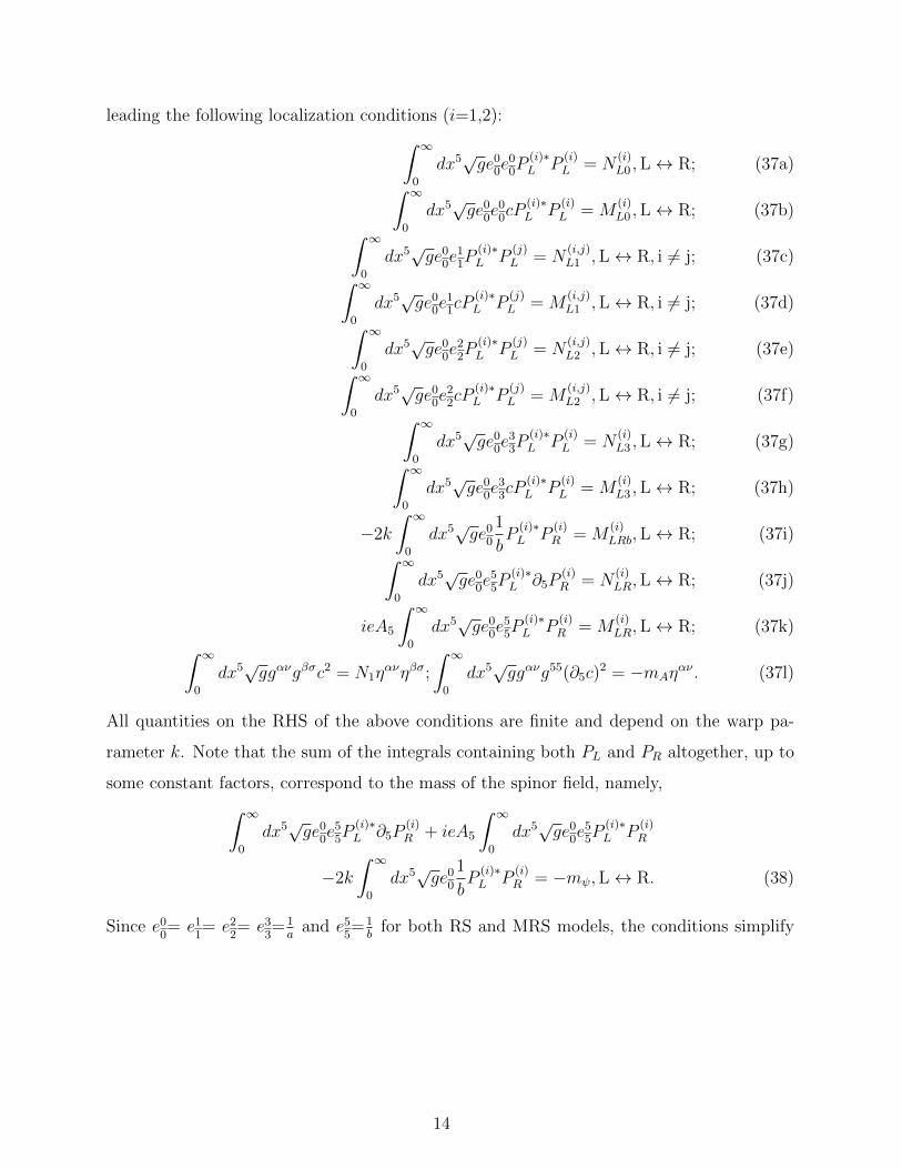
leading the following localization conditions (i=1,2):∫ ∞0

dx5√ge00e

00P

(i)∗L P

(i)L = N

(i)L0 ,L↔ R; (37a)∫ ∞

0

dx5√ge00e

00cP

(i)∗L P

(i)L = M

(i)L0 ,L↔ R; (37b)∫ ∞

0

dx5√ge00e

11P

(i)∗L P

(j)L = N

(i,j)L1 ,L↔ R, i 6= j; (37c)∫ ∞

0

dx5√ge00e

11cP

(i)∗L P

(j)L = M

(i,j)L1 ,L↔ R, i 6= j; (37d)∫ ∞

0

dx5√ge00e

22P

(i)∗L P

(j)L = N

(i,j)L2 ,L↔ R, i 6= j; (37e)∫ ∞

0

dx5√ge00e

22cP

(i)∗L P

(j)L = M

(i,j)L2 ,L↔ R, i 6= j; (37f)∫ ∞

0

dx5√ge00e

33P

(i)∗L P

(i)L = N

(i)L3 ,L↔ R; (37g)∫ ∞

0

dx5√ge00e

33cP

(i)∗L P

(i)L = M

(i)L3 ,L↔ R; (37h)

−2k

∫ ∞0

dx5√ge00

1

bP

(i)∗L P

(i)R = M

(i)LRb,L↔ R; (37i)∫ ∞

0

dx5√ge00e

55P

(i)∗L ∂5P

(i)R = N

(i)LR,L↔ R; (37j)

ieA5

∫ ∞0

dx5√ge00e

55P

(i)∗L P

(i)R = M

(i)LR,L↔ R; (37k)∫ ∞

0

dx5√ggανgβσc2 = N1η

ανηβσ;

∫ ∞0

dx5√ggανg55(∂5c)

2 = −mAηαν . (37l)

All quantities on the RHS of the above conditions are finite and depend on the warp pa-

rameter k. Note that the sum of the integrals containing both PL and PR altogether, up to

some constant factors, correspond to the mass of the spinor field, namely,∫ ∞0

dx5√ge00e

55P

(i)∗L ∂5P

(i)R + ieA5

∫ ∞0

dx5√ge00e

55P

(i)∗L P

(i)R

−2k

∫ ∞0

dx5√ge00

1

bP

(i)∗L P

(i)R = −mψ,L↔ R. (38)

Since e00= e1

1= e2

2= e3

3= 1a

and e55=1b

for both RS and MRS models, the conditions simplify

14

into ∫ ∞0

dx5√g

a2P

(i)∗L P

(i)L = N

(i)L0 = N

(i)L3 ,L↔ R; (39a)∫ ∞

0

dx5√g

a2cP

(i)∗L P

(i)L = M

(i)L0 = M

(i)L3 ,L↔ R; (39b)∫ ∞

0

dx5√g

a2P

(i)∗L P

(j)L = N

(i,j)L1 = N

(i,j)L2 ,L↔ R, i 6= j; (39c)∫ ∞

0

dx5√g

a2cP

(i)∗L P

(j)L = M

(i,j)L1 = M

(i,j)L2 ,L↔ R, i 6= j; (39d)

−2k

∫ ∞0

dx5√g

abP

(i)∗L P

(i)R = M

(i)LRb,L↔ R; (39e)

ieA5

∫ ∞0

dx5√g

abP

(i)∗L P

(i)R = M

(i)LR,L↔ R; (39f)∫ ∞

0

dx5√g

abP

(i)∗L ∂5P

(i)R = N

(i)LR,L↔ R; (39g)∫ ∞

0

dx5√g

a4c = N1;

∫ ∞0

dx5√g

a2b2(∂5c)

2 = mA. (39h)

We could not analyze whether the spinor-vector system fulfill the above conditions until

we look at the field equations. This is because P(i)L,R and c are solutions of the field equations

that correspond to the extra coordinate. Even though the integrands in conditions (39a)

and (39b) differ by a factor c(x5) one could not specify c(x5). c(x5)=const is consistent

with both conditions but this not the only choice. For example, functions c(x5) of the form

c(x5) = 1 + e(x5)a2/(√gP

(i)∗L P

(i)L ) with

√gP

(i)∗L P

(i)L 6= 0 for all x5 and

∫∞0dx5e(x5) = 0

are consistent with the conditions (39a) and (39b). As there are many functions fulfilling∫∞0dx5e(x5) = 0, we understand that c(x5) is not unique. We must look at the field equations

first before going through the localization conditions again.

The field equations corresponding to spinor field are

iΓMDMΨ =1

aiγµDµΨ +

1

bi(−iγ5)D5Ψ,

1

aiγµ(∂µ − iecaµ)Ψ + i

1

aγµ(

ik

2

a

bγµγ5) +

1

bi(−iγ5)(∂5 − ieA5)Ψ = 0. (40)

In the above equations the dependence on the extra coordinate comes from a, b, c and

Ψ. The equations make sense only if all these functions have the form that all terms in

the equations are functions of the extra coordinate which are proportional to one another.

Accordingly the function c(x5) should be a constant. As c(x5) is a constant the integrand

in the first condition (39h) is proportional to√g

a4which is equal to unity for the RS model.

15

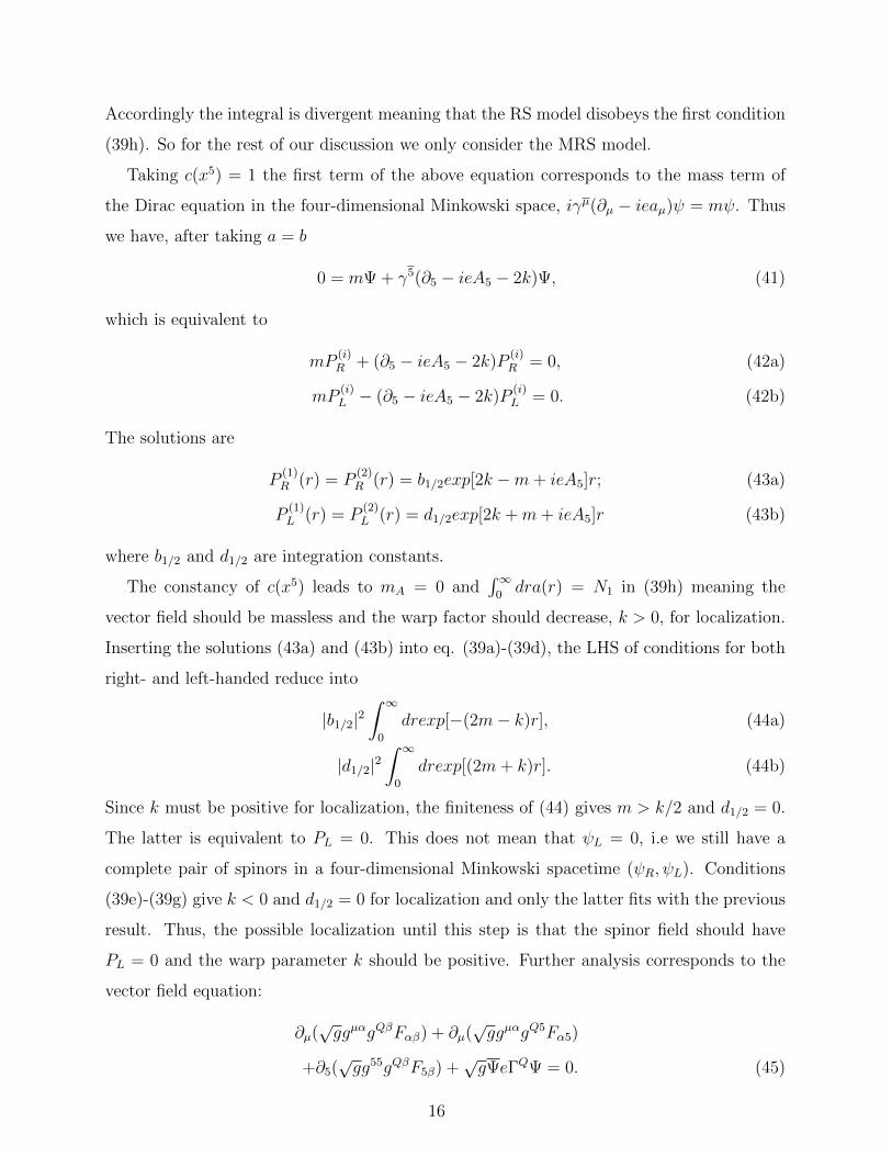
Accordingly the integral is divergent meaning that the RS model disobeys the first condition

(39h). So for the rest of our discussion we only consider the MRS model.

Taking c(x5) = 1 the first term of the above equation corresponds to the mass term of

the Dirac equation in the four-dimensional Minkowski space, iγµ(∂µ − ieaµ)ψ = mψ. Thus

we have, after taking a = b

0 = mΨ + γ5(∂5 − ieA5 − 2k)Ψ, (41)

which is equivalent to

mP(i)R + (∂5 − ieA5 − 2k)P

(i)R = 0, (42a)

mP(i)L − (∂5 − ieA5 − 2k)P

(i)L = 0. (42b)

The solutions are

P(1)R (r) = P

(2)R (r) = b1/2exp[2k −m+ ieA5]r; (43a)

P(1)L (r) = P

(2)L (r) = d1/2exp[2k +m+ ieA5]r (43b)

where b1/2 and d1/2 are integration constants.

The constancy of c(x5) leads to mA = 0 and∫∞0dra(r) = N1 in (39h) meaning the

vector field should be massless and the warp factor should decrease, k > 0, for localization.

Inserting the solutions (43a) and (43b) into eq. (39a)-(39d), the LHS of conditions for both

right- and left-handed reduce into

|b1/2|2∫ ∞0

drexp[−(2m− k)r], (44a)

|d1/2|2∫ ∞0

drexp[(2m+ k)r]. (44b)

Since k must be positive for localization, the finiteness of (44) gives m > k/2 and d1/2 = 0.

The latter is equivalent to PL = 0. This does not mean that ψL = 0, i.e we still have a

complete pair of spinors in a four-dimensional Minkowski spacetime (ψR, ψL). Conditions

(39e)-(39g) give k < 0 and d1/2 = 0 for localization and only the latter fits with the previous

result. Thus, the possible localization until this step is that the spinor field should have

PL = 0 and the warp parameter k should be positive. Further analysis corresponds to the

vector field equation:

∂µ(√ggµαgQβFαβ) + ∂µ(

√ggµαgQ5Fα5)

+∂5(√gg55gQβF5β) +

√gΨeΓQΨ = 0. (45)

16

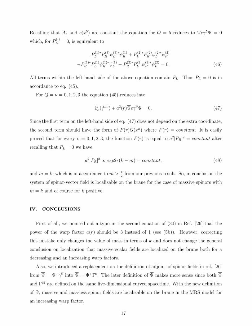
Recalling that A5 and c(x5) are constant the equation for Q = 5 reduces to Ψeγ5Ψ = 0

which, for P(i)L = 0, is equivalent to

P(1)∗L P

(1)R ψ

(1)∗L ψ

(1)R + P

(2)∗L P

(2)R ψ

(2)∗L ψ

(2)R

−P (1)∗R P

(1)L ψ

(1)∗R ψ

(1)L − P

(2)∗R P

(2)L ψ

(2)∗R ψ

(2)L = 0. (46)

All terms within the left hand side of the above equation contain PL. Thus PL = 0 is in

accordance to eq. (45).

For Q = ν = 0, 1, 2, 3 the equation (45) reduces into

∂µ(fµν) + a2(r)ΨeγνΨ = 0. (47)

Since the first term on the left-hand side of eq. (47) does not depend on the extra coordinate,

the second term should have the form of F (r)G(xµ) where F (r) = constant. It is easily

proved that for every ν = 0, 1, 2, 3, the function F (r) is equal to a2|PR|2 = constant after

recalling that PL = 0 we have

a2|PR|2 ∝ exp2r(k −m) = constant, (48)

and m = k, which is in accordance to m > k2

from our previous result. So, in conclusion the

system of spinor-vector field is localizable on the brane for the case of massive spinors with

m = k and of course for k positive.

IV. CONCLUSIONS

First of all, we pointed out a typo in the second equation of (30) in Ref. [26] that the

power of the warp factor a(r) should be 3 instead of 1 (see (5b)). However, correcting

this mistake only changes the value of mass in terms of k and does not change the general

conclusion on localization that massive scalar fields are localized on the brane both for a

decreasing and an increasing warp factors.

Also, we introduced a replacement on the definition of adjoint of spinor fields in ref. [26]

from Ψ = Ψ+γ0 into Ψ = Ψ+Γ0. The later definition of Ψ makes more sense since both Ψ

and ΓM are defined on the same five-dimensional curved spacetime. With the new definition

of Ψ, massive and massless spinor fields are localizable on the brane in the MRS model for

an increasing warp factor.

17

Secondly, we analyzed localizability of interacting fields in the RS and MRS models.

Here, a system of interacting fields is said to be localized on the brane if all the fields

within the system are localized. The system that we analyzed, i.e scalar-vector and spinor-

vector systems in the RS model were not localizable since the localization conditions led the

integrals over the fifth coordinate in the first equation of (17c) for scalar-vector system, in

the first equation of (39h) for spinor-vector system were of the form∫∞0dy which is infinite.

While for the vector-vector system the localizability leads to c(r) = 0 or c =constant with

k = 0. This means that one is not able to define localized YM fields in the RS model.

We looked at interacting fields in the MRS model. A system of scalar-vector is localizable

on the brane since all integrals over the extra dimension from 0 to ∞ are finite. We also

demonstrated that the condition a2χ∗χ=const from the equation of motion for vector field

(25a) gives mass mϕ =√

2k. For a vector-vector system represented by the Yang-Mills field,

we obtained that the system is localizable on the brane r = 0 for the case massless mode

and a decreasing warp factor. Finally for the spinor-vector system, we obtained that the

system is also localizable on the brane r = 0 even though with some restrictive conditions:

the vector field should be massless, the mass of the spinor field should be m = k, PL = 0,

and the warp factor should decrease. Note that PL = 0 does not mean that the field ψL(xµ)

on the brane does not exist.

So, the general conclusion is that in terms of interacting fields, the MRS brane model has

better localization properties than the original RS model: the scalar-vector, vector-vector,

and spinor-vector systems cannot be localized on the brane y = 0 in the original RS model

while these systems are localizable on the brane r = 0 (with some restrictions) in the MRS

brane model.

Acknowledgments

The work of D.W was supported through a 2016 PKPI Scholarship by the Directorate

General of Resources for Science Technology and Higher Education of the Republic of

Indonesia. T and JSK were supported by the Riset dan Inovasi Institut Teknologi Bandung

and the Desentralisasi DIKTI research programs.

18

[1] J. M. Overduin and P. S. Wesson, Phys. Rept. 283, 303 (1997).

[2] M. Gogberashvili, Mod. Phys. Lett. A 14, 2025 (1999).

[3] M. Gogberashvili, Europhys. Lett. 49, 396 (2000).

[4] M. Gogberashvili, Int. J. Mod. Phys. D 11, 1639 (2002).

[5] V.A Rubakov and M.E. Shaposhnikov, Phys. Lett. B 125, 136 (1983).

[6] M. Visser, Phys. Lett. B 159, 22 (1985).

[7] E. J. Squires, Phys. Lett. B 167, 286 (1986).

[8] G. Kalbermann and H. Halevi, gr-qc/9810083.

[9] M. Gogberashvili, hep-ph/9812296; hep-ph/9812365.

[10] A. Barnaveli and O. Kancheli, Sov. J. Nucl. Phys. 51, 901 (1990); Sov. J. Nucl. Phys. 52, 920

(1990).

[11] J. Polchinski, Phys. Rev. Lett. 75, 4724-4727 (1995).

[12] P. Horova and E. Witten, Nucl. Phys. B460, 506-524 (1996).

[13] M. Gogberashvili and D. Singleton, Phys. Rev. D 69, 026004 (2004).

[14] M. Gogberashvili and P. Midodashvili, Europhys.Lett. 61, 308 (2003)

[15] M. Gogberashvili and P. Midodashvili, Phys. Lett. B 515, 447 (2001).

[16] M. Gogberashvili and D. Singleton, Phys. Lett. B 582, 95(2004).

[17] P. Midodashvili, Europhys. Lett. 69, 478 (2004).

[18] P. Midodashvili and L. Midodashvili, Europhys. Lett. 66, 640 (2004).

[19] I. Oda, Phys. Rev. D 62, 126009 (2000).

[20] I. Oda, Phys. Lett. B 508, 96 (2001).

[21] D. Singleton, Phys. Rev. D 70, 065013 (2004).

[22] L. Randall and R. Sundrum, Phys. Rev. Lett. 83, 3370 (1999).

[23] L. Randall and R. Sundrum, Phys. Rev. Lett. 83, 4690 (1999).

[24] B. Bajc and G. Gabadadze, Phys. Lett. B 474, 282 (2000).

[25] A. Pomarol, Phys. Lett. B 486, 153 (2000).

[26] Jones P., Munoz G., Singleton D., Triyanta, , Phys. Rev. D 88, 025048 (2013).

[27] Triyanta, Singleton D., Jones P., Munoz G., AIP Conference Proceedings 1617, 96 (2014).

19

[28] L.H. Ryder, Quantum Field Theory, Cambridge University Press, 1996.

20