Embed Size (px)
Citation preview
Localising Discrete Points in 3D Space using
Stereo Pairs of Digital Slot-scanning X-rays
Susan M Wynne
Submitted to the Faculty of Health Sciences at the University of Cape
Town in partial fulfilment of the requirements for the degree of Master
of Science in Biomedical Engineering.
Cape Town
December, 2006

The copyright of this thesis vests in the author. No quotation from it or information derived from it is to be published without full acknowledgement of the source. The thesis is to be used for private study or non-commercial research purposes only.
Published by the University of Cape Town (UCT) in terms of the non-exclusive license granted to UCT by the author.

M"T lolO. ~~ W'INN
~2~~3~
Declaration
I, SUSAN MARGARET WYNNE, hereby declare that the work on which this thesis is
based is my original work (except where acknowledgements indicate otherwise) and that
neither the whole nor any part of it has been, is being or is to be submitted for any other
degree in this or any other University.
I empower the University to reproduce for the purpose of research, either the whole or part
of the contents of this thesis in any manner.
Signature
Date
ii
Abstract
Obtaining three-dimensional information about the human body through the use of X-ray
stereophotogrammetry provides medical professionals with more information on which to
accurately plan, assess or implement procedures. Such information has been used in
previous studies in order to assess the micro-motion of hip-joint prostheses, scoliosis
treatment effectiveness and brachytherapy seed implantation positioning.
The main objective of this study was to assess the feasibility of using the Statscan low
dose X-ray scanner at the Groote Schuur Hospital, Cape Town for the localisation of
discrete points using X-ray stereophotogrammetry. The X-ray source and detector bank of
the scanner are mounted on a C-arm that travels horizontally to produce X-ray images.
The X-ray beam is fan-shaped as opposed to a conical shaped beam often used in
conventional radiography, which results in magnification of objects in X-ray images in one
dimension only.
To find a suitable stereophotogrammetric technique, traditional and newly developed
methods were explored. The most suitable method for the three-dimensional localisation
of points in Statscan images was established to be one previously developed for
computed tomography scan projected radiographs (surviews), which have similar
geometrical properties to Statscan images. USing information gathered from previous
studies, a calibration frame with radio-opaque markers was designed and constructed
specifically for use with Statscan. The three dimensional marker positions were measured
using a line-of-sight photogrammetric technique and a marker location routine was written
in Matlab to locate the marker centroids on the X-ray images.
Experiments were performed to establish the reconstruction errors and characteristics of
the Statscan set-up using different control point configurations and various X-ray scanning
angles. In addition, reconstruction accuracies when using both extrapolation and
interpolation were assessed.
It has been demonstrated that stereophotogrammetry with the Statscan scanner would be
suitable for applications where errors above 1 mm and lower than 2 mm can be tolerated,
such as cephalometry, brachytherapy planning and assessment of the spine.
Iii

Acknowledgements
This research would not have been possible without the support and contribution of many
people. All those who were involved are warmly thanked for their valuable input and
expertise in their various fields.
My sincere thanks goes to my project supervisors and mentors, Prof C L Vaughan and
Dr T S Douglas, who provided me with support, motivation and guidance throughout this
project and the field of Biomedical Engineering.
Ms G Bowie, Chief Radiographer at the Groote Schuur Hospital, for her assistance in
obtaining the initial Statscan X-ray test data.
Mr M C Briers, Postgraduate Student, Geomatics and Surveying Department, UCT, for his
assistance in calibrating the calibration frame.
Mr J Markus, Biomedical Workshop Artisan, University of Cape Town, for his assistance in
the construction of the calibration frame.
Dr E Meintjes, Senior Lecturer and Scientific Officer, Medical Imaging Research Unit,
UCT, for her assistance in the theory of stereophotogrammetry.
Mr D Moore and Ms R Campbell, Researchers at the Sports Science Institute, for their
assistance in obtaining 3D information with the Vicon measurement system.
Ms V Sanders and Mr S Steiner, Researchers, University of Cape Town, for their
assistance in taking Statscan X-ray images.
Mr D Tabakin, Sport Science Institute, for the measurement of the calibration frame using the Vicon Motion System.
African Medical Imaging (Pty) Ltd for financial support in 2000 - 2001.
My parents, Margaret and David Wynne, my sister, Heather Wynne and my husband, Iwan van Wyk, for their encouragement and patience during the course of this project.
iv

Declaration
Abstract
Acknowledgements
Table of Contents
List of Figures
List of Tables
Abbreviations
Chapter 1 : Introduction
Table of Contents
1.1 Locating Points in Three Dimensions
1.2 Basic Theory of Stereophotogrammetry
1.3 Objectives of the Study
1.4 Scope and Limitations
1.5 Sources of Information
1.6 Overview
Chapter 2 : Reconstruction Methods and Applications in X-Ray
Stereophotogram metry
2.1 Roentgen Stereophotogrammetric Analysis (RSA)
2.1.1 The RSA reconstruction algorithm
2.1.2 The RSA calibration
2.1.3 Accuracy of RSA
2.2 Direct Linear Transformation (DL T)
2.2.1 Overview
2.2.2 DL T Algorithm
2.2.3 The DL T calibration frame
2.2.4 The DL T calibration process
2.2.5 Accuracy of the DL T
2.3 A Two-Dimensional Projective Transformation Method
2.3.1 Overview
2.3.2 The Projective Transformation Algorithm
2.3.3 Calibration for the Projective Transformation
2.3.4 Accuracy using the Projective Transformation
ii
iii
iv
v
viii
xi
xii
3
5
6
6
6
7
9
10
11
13
15
15
15
17
18
19
22
22
23
23
23
v

2.4 The Non-stereo Corresponding Point Method (NSCP) 24
2.4.1 Overview 24
2.4.2 The NSCP algorithm 24
2.4.3 Accuracy of the NSCP method 25
2.5 Image Marker Identification used in Previous Studies 25
2.5.1 Identifying the two-dimensional marker positions 25
2.5.2 Locating the Marker Centroid 26
2.6 X-Ray Stereophotogrammetric Applications 28
2.6.1 Migration Assessment 28
2.6.2 Spinal Assessment and Treatment Planning 29
2.6.3 Radiation Oncology 30
2.6.4 Cephalometry 30
2.6.5 Additional Applications 31
Chapter 3 : Materials and Method 32
3.1 Statscan Materials and Technical Apparatus 32
3.1.1 The Statscan Digital Scanner 32
3.1.2 Statscan Digital Radiographs 33
3.1.3 The Computer Equipment 34
3.2 Method of X-ray Stereophotogrammetry used with Statscan 34
3.2.1 Stereophotogrammetry technique suitable for use with SPRs 34
3.3 Calibration Equipment 35
3.3.1 The Calibration Frame Design 35
3.3.2 The Calibration Frame Survey 40
3.4 Image Marker Centroid Location 41
3.4.1 Calibration Frame Marker Centroid Location 41
3.4.2 Phantom Marker Centroid Location 44
3.5 Reconstruction Software 46
Chapter 4 : Experiments and Results 47
4.1 Reproducibility of the 2D marker centroid location 49
4.1.1 Results: Reproducibility of 2D marker centroid selection and co~~ G
4.2 Reconstruction of control pOints 50
4.2.1 Description of the control point sets for control point reconstruction 51
vi

4.2.2 Results of control point reconstruction 52
4.3 Reconstruction of test points using calibration frame markers 55
4.3.1 Description of the control point sets for test point reconstruction 55
4.3.2 Results of test point reconstruction 56
4.4 Reconstruction of test pOints using extrapolation 59
4.4.1 Description of the control point sets for extrapolation 60
4.4.2 Results of pOint reconstruction using extrapolation 60
4.5 Reconstruction of phantom pOints using interpolation
4.5.1 Description of the control point sets for phantom marker interpolation
4.5.2 Results of phantom marker interpolation
Chapter 5 : Discussion
5.1 Equipment as a Possible Source of Error
64
66
66
69
69
5.1.1 The Calibration Frame 69
5.1.2 The Digital Imaging System 71
5.2 The effect of calibration variables on reconstruction accuracy 72
5.2.1 The reproducibility of two-dimensional marker identification 72
5.2.2 The effect of separation angle and scanning angle on reconstruction accuracy 73
5.2.3 The effect of the number of control pOints on reconstruction accuracy
5.2.4 The reconstruction accuracy when extrapolating
5.2.5 The reconstruction accuracy when interpolating
5.3 Applications for the use of Statscan Stereophotogrammetry
Chapter 6 : Conclusions
Chapter 7 : Recommendations
Appendix A: Measured Calibration Frame Marker Coordinates
Appendix B: Measured Phantom Marker 3D Coordinates
Appendix C: Matlab Software Code
Appendix D: Experiment Data Tables
Appendix E: Additional Extrapolation Experiment Details
References
75
79
82
83
86
88
89
91
92
94
99
104
vii

List of Figures
Figure Description Page
1.1 An early 1900's X-ray stereogram of a gunshot wound in the foot 1
(Judge, 1926)
1.2 An example of automated RSA software (DI RSA) showing knee 3
prostheses with RSA markers identified on a digitised X-ray image
(RSA-CMS® product brochure, 2005)
1.3 The stereopsis of human vision (adapted from Moffit, 1967) 3
1.4 An example of a full-body digital Statscan X-ray image of a trauma 4
patient with multiple injuries (Beningfield et al., 2003)
1.5 Statscan C-arm and patient trolley 5
2.1 A typical X-ray set-up illustrating the effective focal point and the image 7
distortion phenomenon (adapted from Slama et al., 1989)
2.2 Illustration of the imaging geometry of (a) 3D conventional X-ray cone, 8
and (b) Statscan or computed tomography 2D X-ray fan-beam
2.3 Two Statscan images showing the distortion of spherical ball bearings 8
of the same size depending on the distance from the X-ray detectors:
(a) The ball-bearing closer to the detector, (b) The ball bearing further
away from the detectors. The distortion is most prominent in the image
x-direction
2.4 The object space and image plane can be related by using the co- 16
linearity assumption and vector algebra (Adapted from Mitton, et al.,
2000)
2.5 A Statscan image of the spine of a 13 year-old girl with scoliosis 29
3.1 The Statscan Digital X-ray Scanner with global coordinate system 32
3.2 The dimensions of the Statscan machine and the height of the trolley 36
limit the imaging space and provide constraints for the design of the
calibration frame
3.3 (a) Illustrating how an image could be truncated if the frame is outside 37
the X-ray fan-beam. (b) A good image is obtained when the frame is
within the X-ray beam.
3.4 The pyramid-shaped calibration frame with twenty-five radio-opaque 38
markers
3.5 The calibration frame viewed from above. The numbers indicate the 38
marker position labels.
viii
3.6 One of the calibration images used to measure the three-dimensional 39
position of the markers accurately.
3.7 An X-ray image of the calibration frame with the phantom object in the 40
centre during marker identification. The Matlab program requires user
intervention to select the calibration frame markers in the correct order
using the mouse and a cursor. Once selected, the marker is labelled
as shown.
3.8 Examples of marker centre correction on two calibration markers 41
imaged at an angle of 90°
3.9 A marker imaged at 90° where the hole through the ball-bearing is 42
visible. The outer black square is the user-selected point and the
central black square is the position found by the centre correction
algorithm.
3.10 Overlapping markers on Statscan images taken at goo. The outlying 42
black SQuares are the user-selected points and the "corrected" or more
central black squares are the pOSitions found by the algorithm.
3.11 The pixel intensity values on opposite edges of a marker showing the 43
symmetrical intensity drop from 225 (marker) to about 30 (non-marker)
over 6 pixels.
3.12 The Perspex phantom frame used for experiments involving 44
reconstruction of unknown points using interpolation
3.13 An anterior-posterior Statscan X-ray of the ring phantom. Each marker 44
(small white dot) has been labelled for ease of identification. The large
white objects are the Perspex columns X-rayed through their length.
3.14 The marker centre correction of a 1 mm steel marker embedded in a 45
Perspex rod. The outer black square is the user selected point and the
central square is the corrected centre.
4.1 Explanation of how the images taken at seven different scanning 46
angles are paired to form 21 combinations at six separation angles
4.2 Image-set A - Mean absolute errors for the reconstruction of control 52
point sets 21 (0); 16 (0); 11(il); 7(+) control points.
4.3 Image-set B - Mean absolute errors for the reconstruction of control 53
point sets, 21 (0); 16 (0); 11 (il); 7 (+) control pOints.
4.4 Mean absolute errors for the reconstruction of five unknown test pOints 56
when using 16 (0); 11 (il) and 7(+) control points.
Ix
4.5 The mean absolute X, V and Z errors for the reconstruction of 5 test 57
points using 16 control points in different configurations; configuration
1 (0), configuration 2 (0), configuration 3 (~), configuration 4 (+)
(Configurations defined in Table 4.5).
4.6 An illustration of the effect on the C-arm scanning angles that form the 58
separation angle of 150 on X (0), V (0) and Z (~) mean absolute errors
when reconstructing 5 test points using 16 control points in
configuration 1.
4.7 The mean absolute errors for the reconstruction of X (0), V (~) and Z 60
(+) coordinates of five test points when extrapolating in the (a) X, (b) V,
and (c) Z directions.
4.8 The resultant errors for the reconstruction of five test points when 61
using extrapolation in the (a) X-, (b) V- and (c) Z directions.
4.9 An illustration of the effect of C-arm scanning angles that form the 62
separation angle of 150 on the X (o),V (~) and Z (0) mean absolute
errors when extrapolating in the (a) X- (b) V- and (c) Z-directions
4.10 The phantom within the calibration frame on the patient table of the 63
Statscan machine, Groote Schuur Hospital.
4.11 A pair of Statscan images where the phantom was radiographed within 64
the calibration frame at 00 and 450 respectively.
4.12 X-, V-, Z- and resultant absolute mean errors for the reconstruction of 66
five phantom points using different control point sets 16 (0); 11 (~); 7
(+) control points.
4.13 A three-dimensional plot of the 25 frame markers (~), 11 labelled 67
control points (+) and the 5 interpolated pOints (0) within the calibration
frame space.
5.1 A graph of the resultant mean absolute errors for the reconstruction of 75
control pOints (0, experiment 4.2) and test points (0, experiment 4.3)
versus the number of control pOints used while using a 900 separation
angle and image-set B in each case.
5.2 A plot of the results of a previous DL T study showing mean absolute 76
errors for control pOints and non-control test pOints using various
numbers of control pOints (Hinrichs and McLean, 1995)
5.3 A plot of the mean absolute Z-errors from the reconstruction of five test 80
points when extrapolating in the V -direction using 11 control points
(configuration 1) and a separation angle of 150 versus the pairs of C-
arm scanning angles.
x

List of Tables
Table Description Page
2.1 Accuracies of a selection of previous RSA studies and their 13
separation angles
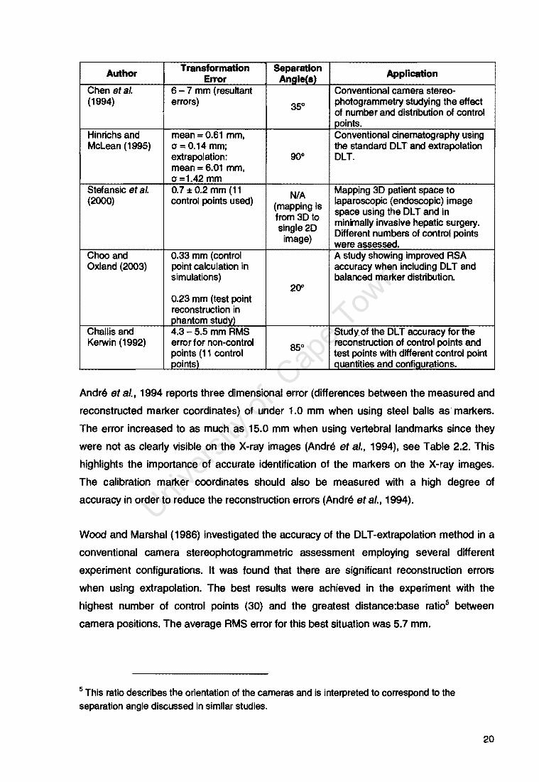
2.2 Three dimensional error of a selection of previous OL T studies. a = 19
standard deviation; RMS = root mean square.
2.3 Comparison of CT slice coordinates and those calculated from the 23
SPRs
4.1 Manually corrected markers in image-sets A and B 46
4.2 The mean standard deviations for the 20 coordinates of the markers 49
identified manually and using the marker correction program
4.3 The mean standard deviations for the reconstruction of 3D 49
coordinates of the markers identified manually and using the marker
correction program
4.4 The marker sets used to test the transformation by reconstruction of 50
control points
4.5 Marker sets used to test the unknown point transformations 55
4.6 Marker sets used to assess the transformation for use in 59
extrapolation.
4.7 The manually corrected and excluded phantom markers 65
4.8 Marker sets used to assess the transformation for interpolation with a 65
phantom
xi

ACL
CCD
CT
DICOM
DLT
DPI
FCP
GSH
ILUT
Ip/mm
Matlab
MOLT
MeV
MRI
NAC
ROI
RSA
RSA-CMS@
SO
SPG
SPR
THR
~Sv
Abbreviations
Anterior Cruciate Ligament
Charge Coupled Device
Computed Tomography
Digital Communication format for Medical use
Direct Linear Transformation
Dots Per Inch
Fiducial and Control Plane
Groote Schuur Hospital
Input Look-up Table
Line pairs per millimetre
"Matrix Laboratory" programming and computing tool
Modified Direct. Linear Transform
Mega electron Volts (1 X 10⁶ eV)
Magnetic Resonance Imaging
National Accelerator Centre
Region 01' Interest
Roentgen Stereophotogrammetric Analysis
Radio Stereometric Analysis - Clinical Measurement Solution
Standard Deviation
Stereophotogrammetry
Scan Projected Radiography
Total Hip Replacement
Micro-Sieverts
xii
Chapter 1 : Introduction
1.1 Locating Points in Three Dimens ions
There are many areas in engineering and medicine where locating discrete points In three·
dimensional space Is extremely valuable. Three·(!imensionallmaging techniques, such as
Computed Tomography (Cn and MagnetIC Resonance Imaging (MAl). have become
standard medical imaging tools around the world. SterllQPhotogrammetry is another
method of locating pointS In three dimensions.
Stell~ophotogrammetry IS a method 01 obtaining spatial data (X. Y and Z point cOOfdlnatesj
of objects from Iffiages of lhe objects uSing the two-dimensIOnal • . y Image coordinates
(van Geems, t991). The Slereophotogrammetry techrnque IS widely used in land
surve-,'lflQ. where the contours of the land are calculated Irom O'IIet1applng planar Images
of the land (Judge, 1926; MotIit. 1967; Haller!. 1960). SImilar tachniques can be used to
find Ihree-dimenslonal mformallOO of OOjects f rom stereo images.
For medical applications, stereophotogrammel ry can be performed using X·ray Images 10
prOYide the three-dImensional Information 01 Internal structures. Finding the spaBaI
coordinates of points from stereo X·rays has been an area of interest since liS early as
t897, two years allor Roentgen discovered X-rays (Selvik et al" 1983).
In early studies, the X-ray Images were viewed using stereoscopes and three-dimensional
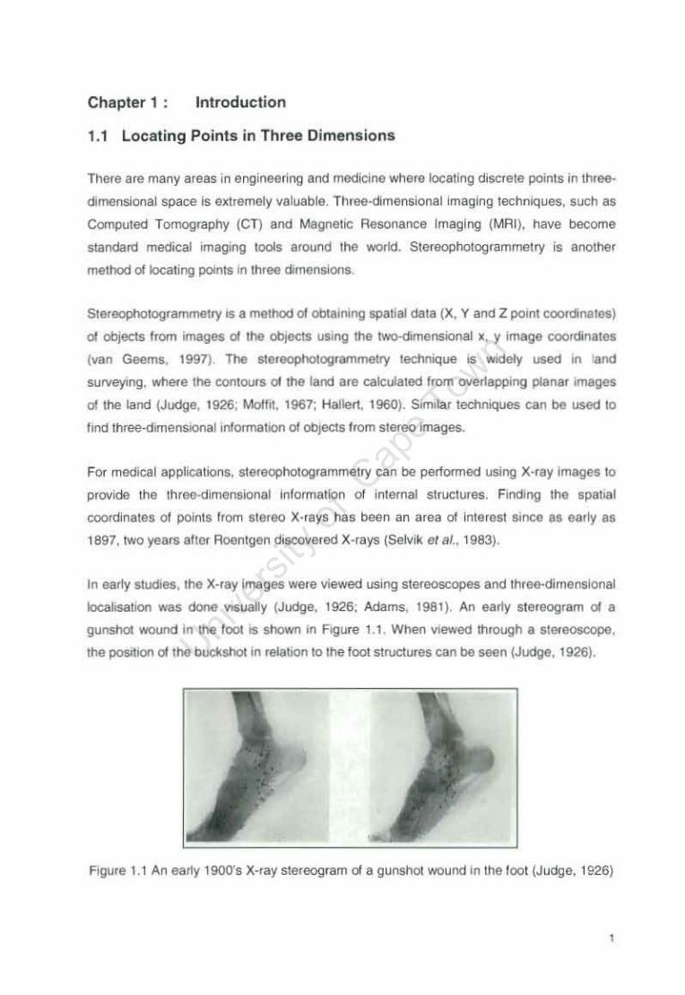
localisation .... as done VlSua8y (Judge, 192t>; Adams, 1981). An early stereogram of a
gunshcl wound In the !OOIIS shoWn In Figure 1.1. When viewed lttrough a stereoscope.
the po5Iuon of the bucksholln relauon to Ihe loot structures can be sean (Judge, 1926).
Figure t .1 An early 19OO's X-ray stereogram 01 a gunshot wound In the loot (Judge. 1926)

As computer technology advanced and more studies were done uSing stereo
phOlogrammetry based on photographs. a number 01 techniques were developed to localO
th ree-dimenSional coord inates 01 pornts I rom stereo X-rays. Most 01 the early
development In th iS area was done in the held 01 or1hopaedics With Ihe development 01
Roentgen Slereo·photoglammetnc Analysis (RSA) RSA IS used to assess the relative
motion 01 Iho skeletal system. lor eKample the hip jrnnt. using Implanted markers (Ojan ot
al .. t967: Selvlk el al., 1963). X·ray 51ereo-photogrammeurc studiOS have since eKtended
into a multitude 01 different fields Including rad iat ion oncology tor radia tion therapy
poSlloonmg (Lam and Ten Haken. 1991: Gall el al .. 1993). the assessmenl 01 prosthesis
stability and migration (Ojarl el al., 1987: Va lstar or al .. 2002). the evaluation 01 spinal
disorders (Aubm el al., 1997; Pet it el al., t998; Benameur 01 al., 2003), source localisallon
,n brachytherapy' (LI er al .. 1996; Cal et al .. 1997; BlCe el al . 1999), cranlolaciaf
reconstruction (Baumrind 01 al. t 983) and cranial grOW1h assessmelll (AJberius 01 ai ,
1990)
The labollOlJs traditional X-ray storeophotogrammetry that reqUIred manual marl<er
IdeJ1llficat:on and manual calcu lat ion 01 coordinates prompted the developmelll 01 mare
effic ient systems through the use of compulers. Researchers rntroduced a level 01
automatIOn Into X- ray stereophotogrammetry by usmg digitised X-ray films (Adams and
Constant. , 988) and digital image proceSSing techniques for marker idenill ication
(Ostgaard el al .. 1997: Vrooman 01 a/ 1998).
In addition, researchers have performed studies uSing d,fjerent types 01 reconstruction
algonthms and callbratron frames on order to increase the scope ot applICat ion of X-ray
shlreophotogrammetry and to Improve the accuracy and elflclency oithEr method
Products for use in clinical applications have also become avai lable 100Iowrng X-ray stereo
photogrammetry research, such as 1he RSA-CMs" (RSA Clin ical Measurement Soluhonl
automated measurement software developed in conlunct ion WIth Leiden Uni~efsity. The
Netherlands (Vrooman el al.. 1998) and the Umea RSA system (Blome<ilcal Innovations
AS), developed In conlunctlon With Lund Univers ity. Sweden (Bragdon el al .. 2003). Figure
1 2 shows an eKample 01 automated RSA soltware show,ng knee prostheses wrth RSA
ma r~ers identified on a dig,IISed X-ray Image .
. The treatment 01 cancer through the use 01 implanted tad ioact i~o beads
,
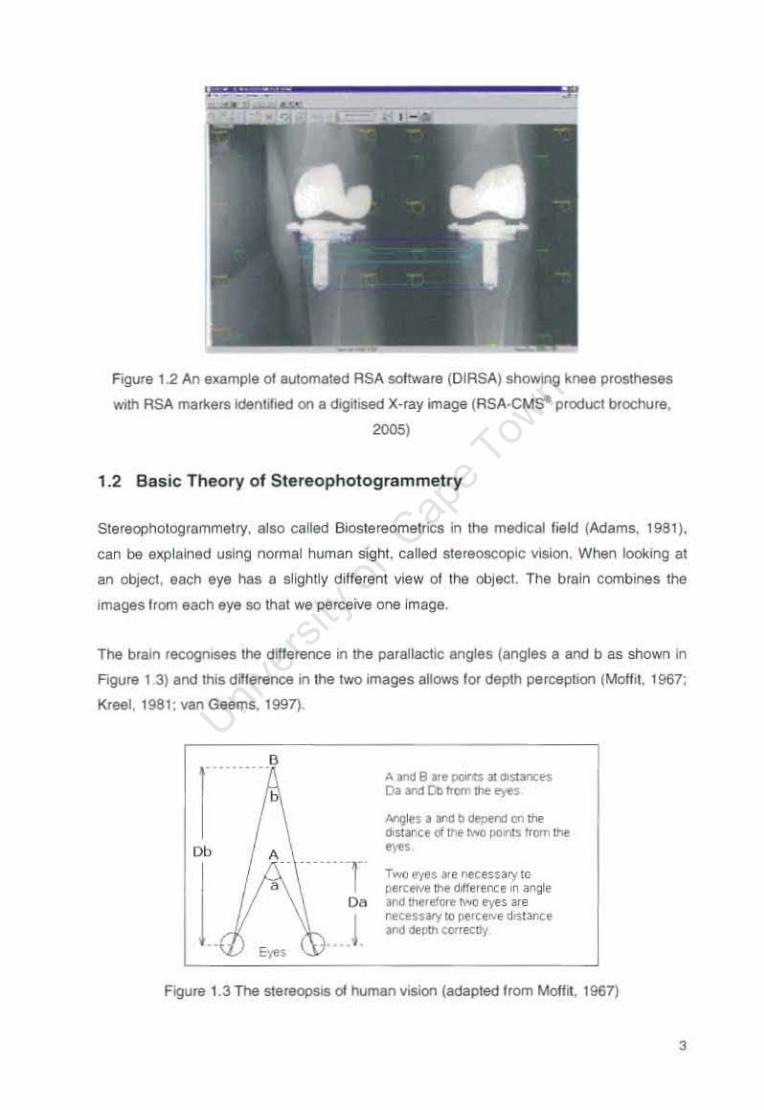
Figure 1.2 An example at autometed ASA solIWare (DIRSA) showing knee prostheses
Wlih RSA mal1<ers identified on a digitISed X-ray image (RSA.CMSS product brochure,
2005)
1.2 Basic Theory of Stereophologrammetry
Stereophologremmetry, elso celled BI05tereometncs in the medlcallield (Actams. 1981 ),
can be explained using normal human sight. called slereoscoplc vision. When looking at
an object. each eye has e sl~htly dtfferent view 01 lhe object. The brain combInes the
images Irom each eye so that we perceive one image.
The brain recogntses the dlllerence in the parallactic engle5 (angles a and b as shown In
FlQure I 3) and this ditierellCEl in the two images allows lor depth perception (Moffit, 1967;
Kreel , 1981 ; van Geems. 1997) .
.. .. 0
Db
A IIIId B .e oooru • dlstantn 01 .-.:I DtI Iro;n"llhe eves
""'gln I a'Id b depenIl 0r'I1Ilo! dlstanee 01 tne IWCI pam "om the .,., T"MJ ~S.! "",esslry lO parcfM! 1t>e dll!r e-nce 111 artille 1or\II ~r"QI'. IWCI ~ are "eensitY III petcerve Osla.nce ....:I ~p!II '01'11(11"1
figure 1.3 The stereopsis of human VISion (adapted Irom Motfil. 1967)
3
Just as two Iyes arl reql,lired to perceive depth correctly. stereophotogrammetry requires
two stightl)r dltterent images 01 an object to be able to obtain three·dimenSlonallnformation
{van Geems. t997}.
In conventional stereophotogrammetry, pl'lolography Is used to obtain two-dimensional
Images 01 an object wilh unknown dimensions. taken from dliterenl angles_ The three·
dimenslOl18t positlOll at o/Jtect POints can be tound if the relahonship between the image
views is known. This Is <iltlmMed through calibfation using a calibration object wtlich has
prevlouslyoetermlo9d. known coordinates. Measurements 01 corresponding landmarks or
mar1<.ers are then taken trom the Images and the photogrammetry process is used to
IranslOlTTl TWO-dImensional COITespoodlng points Into three-dimenSional coordinates
(Adams. t981).
Similarly, X·ray stereophotogrammelry uses two-dimensional X·ray Images to locate the
coordinates 01 specific points in thr"-dimensions. The two-dimensIOnal limitations of
convenllooat X·rays are OVercoml and accU"ate three-dimenSIOnal measurements of
internal strUCTl.l(es can be Iounct. This re<:onstftlC1ion can e~her be done optically by
viewing Itli lmages through e slereosoopEl or mattlematicaUy (Veress. 1989).
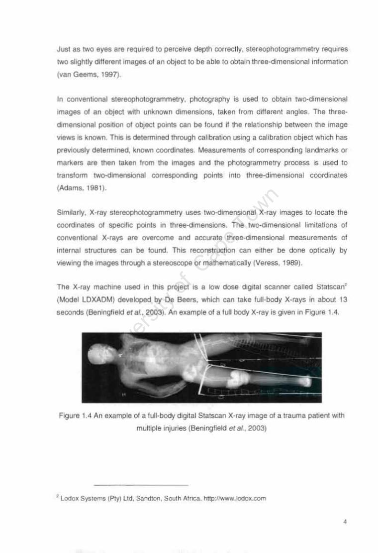
TI'H!I X-ray machine used in this project is a low dose i;lgltal scann8f caltecl Slatscan'
(Model lDXADM) developed by De Beers, which can take futl·body X·rays in about 13
seconds (BenJnglield er al .• 2003). An example 01 a luU body X·ray is given in Fig l,lre 1.4.
Figure 1.4 An example of a full·body dig~al StatsCan X·ray Image 01 a trauma patlenl ....,lh
multiple injuries (Beningiield et a/ .• 2003)
t Lodox Systems (Plyl lid. S;.indtOll . Sooth Africa. hTlj):/Iwww.Iodox.com
•

The Statscan X-ray source and detectors aro mounted on a rotat ing C-arm so that Images
can be laken from angles between 0 and 90' (see FIgure t 5 below) The X-ray source
emits a coll imated fan-beam 01 X-rays as Ihe C-arm moves hOfllontally.
Figure 1.5 Statscan C-arm and patient tro lley
The abi lity to take X- ray images from different angles without moving the obJe<;t or patlen!
makes Stalscan SUitable for perlormrng X-ray stereophotogrammetry to local!! dlscrote
pOInts. One must bear In mind that 11 volume could not be found accura tely With only two
X-ray Images be<;ause the volume would not be accurately represented With such limited
views. Nevertheless. a marker"s three-dimensional coordmales can be found Since It can
be represented as a discrete pOInt and not a vo lume.
1.3 Objectives of the Study
The obje<;tlv(lS Of th iS project were the lollowlng:
1 3.1 Explore traditional and recent stereophotogrammetric techniques to cal ibrate
stereo X-ray Images for the three-dimensional reconstruction of image points
1 32 Invesligate mathematical methoos fo r the three-dimenSIOnal reconstrucllon 01
Image pOints.
1 3.3 Il lustra te the feasibil ity of uSing stereophotogrammetnc technIQues on Images
produced by a low dose digital X-ray imaging system called Statscan.

1.3.4 Determine the optimum con1ig~etlon lor perlorming stereophotogrammelry and
detenT1lrle the reconstruc11OrT errors althe method.
1.3.5 Determll'le clirucaJ applications 10f which the stereophOtogrammetry melhod wot.Ild
be SUItable.
1.3.6 PrOYide conclUSIOnS and recommendationS!Of turther studies.
1.4 Scope and Limitations
The prqecl Is limited to experiments uslng Slatscan digital X-ray Images that were
obtained Irom the Groote Schuur Hospital (GSH) Trauma Unit machine.
1.5 Sources of Information
Through Ihe course 01 this projecl members 01 vanous University departments were
consulted for assistance and advice. These Inchx:!ed members of the Department 01
Biomedk:al Engineering, o.gital Image Processing group in the Depanment of Eleelneal
Englneenng, and the Geomatic:s Department. In addition, specialists Irom the Trauma Unil
al Groote Schu~ Hosp~al and De Beers were also consolted. The individuals Involved
have been acknowtedged in the retevant sectlOl'l of tillS report.
1.6 Overview
Chapter 2 prOYides a re.,;ew at the relevant literature where the methods and applicatIOns
01 previous X--ray stereophologrammelry studies are discussed.
Chapter 3 provldas a descflplion of the pr~ect malerials and methods. The materials
Include the StalSCan digital X-ray scanner and the computer hardware and solrware. The
method ,ncludes a cletailed descrip tlOll of the transtormation algorithm, the calibrahon
Irame design and digital Image processing used in the three dimensional reconstruction of
discrete points. Chapter 4 describes the e~perlmenl s perlormed and the results obtained.
The results are evaluated and compared to the literature in Chapter 5.
Finally. conctuslons are drawo and recommendations fire made in Chapters 6 and 7.
,
Chapter 2 : Reconstruction Methods and Applications in X-Ray
Stereophotogrammetry
A selection of three-dimenslooal rec:oostructoOn methods. chosen basad on thell retaYarx:e
to X-ray and biomecflCal applications. were stlOied In OHler to determine whICh method
would be most appropriate lor use with Statscan Images. There are a lew obvious
dif1er8f'lCes between convenuonal and X-ray stereophotogrammetry Since X-ray Images
have different characteristics to photographic images X-ray images ale generated by
projoc'\lng X-rays lrom a local point in a generallng tUbe. through an object to be Imaged
and onto a l ilm (Slama el.'._ t98O). or In the digital case. on to detectors.
The X-ray image can thuS be described as a shadow 01 the object COI'respoodlnQ to Us
density (Veress. t989). The X-ray local point depends on the dimenstOns 01 the X-ray
source. whICh has a filllie sIZe. However. the ellectlV8 focal point is tlescnbed as a potnt to
allow the use 01 cenual prOjectiorl, where any potnt iflthfee dimensiOnal space lies on a
straight line between the Pfotected poMll on an image plane aM the source. Ftgure 2. 1
depicts an X-ray set-up shoWing the eftectlve local POIIIl. In the mathematICal descnption
of Image generalton, and In practice, it is assumed thallhe X-ray stereophotogrammetry is
based on perfect central projecllon. and therelore no COllectionS are made lor focal POlO!
length (Veress, 1989; Slama at al., 1980).
tmage distortton can be eKpjainad by Figure 2. 1 since It IS clear that the Image 01 the
object will be larger than the real Si~e 01 the object (Slama et 81 .• 1980). The amount at image distor1iOn depends on the position 01 the object between the focal point and the
X-ray film or detectors.
Fout POll'lt
ObJect B 15 " 1I 1ugile. ,I_lOtI than obJKl A 3IId I .... flUJh III a taorve. Im.,g, on the X· tay film for OOJKI B
X-lly (ilm Ot dil1O!"ClotS
W,dlh oflh, X-tay ""0198 of t ach obJ"':!
Figure 2 1 A .yplcal X-ray sel-up lIIustraling 1he eNecllve focal point and the image
distortion phenomenon (adapted ' rom SJama el al" 1989)
1
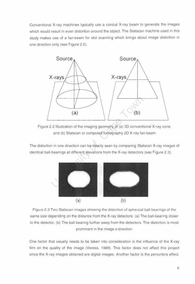
Con~enllOnal X-ray machmes typ ically use a conical X-ray beam to generate Ihe images
which would resu lt in even distortion around the object The Statscan machine used In th is
study makes use of a fan-beam for slot scanning which bnngs aboot Image distort ion in
one direct ion only (see Figure 2.2).
Source
x-rays! 1\, X-rays
/ \ '\
(a) (b)
Figure 2.21 1lustratloo oj the imaging geometry 01 (a) 3D conventional X- ray cOIle.
and (b) Statscan or computed tomography 20 X-ray fan-beam
The distortion In one direction can be clearly seen by comparing Statscan X-ray Images of
identical bali-bear ings al different etevatlons from the X-ray detectors Isee Figure 2_3).
(h)
Figule 2.3 Two St'-'ts~n images ~how l ng the dl~hm",n 01 spher lC<lJ bat l be(lnng~ 01 the
same size depending on the distance from the X-ray detectors: (a) The ball-beanng closer
to the detector, (b) The ball bearing further away Irom the detectors. The d,storl,on i~ most
prominent in the image ~-dlfection
One factor thai usually needs to be taken into considerat ion Is the inlluence of the X-ray
!ttm on the qualIty 01 the image (Veress, t989)_ ThiS factor does not affect thiS project
Since the X-ray Images obtained are d'gital,mages. Another factor is the penumbra ei1ect,

also ceHed Imege degradation. whICh creates a SOit edge 00 objects being X-rayed, and is
due to the geometry al the X·ray machine and the IInlte focal pOlntlangth (Varass 1989:
Slama eta/ .. t9801· This effect is Oescribed In more detail in Saclion 3 4. t . The penumbra
e!1ect is considered neg~gjb~ par1lcular~ becal.lSl:l !he Image oo,ect IS bigger than the
ac1l.lal ot/tect, eod th8felore It Is said to have no effect on measurements taken Irom an
X·ray image, as any meaSl.lrement ml.lSl lake magnification inlo account (Sjama at al.,
1980: Veress. t 989) .
When laking stereo· lmages, It is ot vllal Importance Ihat the object or pelienlis not moved
With respect 10 the ca libration object between scans. If the patient moves. errors wil l be
Introduced that Wil l destroy the ab il ity to perform three-dimensional transformalions
correctly (Slama al al" 1980, Veress, 1989)
2.1 Roentgen Stereophologrammelric Analvsis (RSA)
Roentgen Siereophotogrammetric Ana~sls (RSA)' was developed by Goran Setvlk fn
t974 (Setvlk. t989) in order to have a method o! analysing orthopaedIC treatments such
as prosthetic Implants norHnvasjvely throl.lgh medical Imaging. USing RSA, the three
d imensional coordinates of radio·opaque points can be found trom two·d imenSlOnal X-ray
Images. This method is sometimes referred to as a IIducl<Il and COfil lol plane (FCP)
lechntque due to the use 01 two planes bordering the object for Iha cal ibration (Choo aod
Oxland, 2003). Based on the numerous SwediSh biomechanlcal sll.ldles that have been
conducted I.ls ing thIS method. It can be concluded tMt this method is considered to be the
gold· standard at X-ray stereophotogrammetry in \t1e fie ld at orthopaedics In Sweden and
other SCandinavian countries
The RSA method as described by SelVlk (1989) ceo be sUllVllallSed as tallows:
• RadlO'opaque markers (object markers) are lIlserted Into an ClbJect (e.g. po-osthetic
hip JOint).
• The obtect with a calibratIOn frame Is radtOgraphically exarmned from different
angles. The frame has sovelat callbrallon markers Wlth known coordinates IM.t are
restncled to MuclaJ and contrcll planes (FCFs) to pl"ovide a fI~ed standard at
,
•
referer1Ce for compansor\. The exarnlrlallon could either be performed m an
Inlerpolalion or eKtrapolatiOl1 configuraHon.
• Oblect and ca libration marllers are identilied from the X-ray images_ The two
dimensional Image coordinates 01 lhe calibration mar1<ers. logelher wuh thei r pre
determined 3D coordina tes. determine the translormalior'lS fram 20 images !O 3D
space.
• Object marker Iocal>ons afe calculated In 3D using reconstruction algorithms
2.1 .1 The RSA re.::onslruclion algorithm
The RSA reoonst ructl()(1 method uses the same reconstruCllOrl pr inciples as used In
con~enllonal stereophotogrammetry except that X-rays are used Instead 01 ~i slb le light
(Selvlk, t 989). Since the X-rays are riot detlected in any Significant way When paSSing
through an object, a slralghHorwilrd mmhemancal central proJectlor1 car1 be used (5elvlk,
19891_ 1r1 the RSA method, the X-rays rad iate from the source to form ar1 eJlective cone
shape It Is Important to note that the Slalsear1 scar1r1er does I'\Ot have thiS property (see
Figure 2.21.
To be able to cakulale the three dlmer1S1Onal coordinates oj the markers. the measured
Image coord inates have to be transJormed to the liduc,al plane (lower plar1e of the
calibration frame). The formu lae that provide the relauonshlp between the Image
coord,nates (.I ' _ y') and hduclat plane coordinates ( l. \) are (Selvlk. 1989) '
where '
IJ, .h, .d,. (/1.h).d" /I.-h. x. )' x '. y'
.I" = a IX'+/I,y'+d ,
a,.('+b.y'+1
(/,x'+b. r'+d, - _. .
,,,
I')
project ive transJormallOr1 parameters
calibration mf\rker fidUCia l plar1e co-ordmates
corresponding marker ,mage co-ordinates

A calibration plane with fiducial (calibration) markers in known positions (x, y) is used
together with the image coordinates of the markers (x't y') to solve for the eight unknown
transformation parameters in these equations and this determines the central projection.
Typically nine fiducial markers are used; therefore the system is over-determined and the
eight parameters can be found by the least squares method (Selvik, 1989).
Each ray, R is a straight line given by the formula:
R=I'; +k(1'; -1';') (3)
Where:
I'; fh control point
I'; I the" control point's projection to the fiducial plane
k a real value (for any real value of k, R would be a point on the line)
Another plane with control markers is required to determine the X-ray source focus. These
two planes are fixed together to form the rigid calibration frame or cage that is described in
the next section in more detail.
2.1.2 The RSA calibration
The calibration frame provides key information about the transformation from two to three
dimensions. The calibration frames or cages described in the literature were typically
designed specifically for the required application. For example, in some cases, the study
required the patients to be in a fully weight bearing position within the calibration frame
(Kiss, 1996; Alfaro-Adrian et al., 1999), while others required the patients to be in supine
and then erect positions (Cnsten et al., 1995; Johnsson, 1999). These requirements
dictated which type of calibration frame was used. However, regardless of the application,
the fundamentals of the calibration frame remain the same. A radiolucent frame with radio
opaque calibration markers (contr01 and fiducial markers) at known positions on fiducial
and control planes is required (Selvik, 1989). The fiducial plane is the plane closest to the
radiographic film to define the three-dimensional coordinate system. The points on the
fiducial plane are typically distributed symmetrically and cover the area of interest. The
control plane is the plane further away from the radiographic film and is used to determine
the position of the Roentgen foci (Valstar, 2002). The pOints on the control plane are
11

typically distributed evenly in lines however it is not necessary for these points to cover the
volume of interest.
The RSA transformation algorithm requires the markers to be on mathematical planes;
therefore the calibration frame has to be made from flat material to reduce errors. In the
earlier studies reviewed, the calibration frames were made from a type of acrylic plastic,
e.g. Plexiglass, although this material is not perfectly flat (Karrholm ef al., 1989; Ryd et al.,
1986). In further support of the use of Plexiglass for use in a calibration frame, the
refraction of X-rays through a thin Plexiglass plate is said to be completely negligible
(Veress, 1989). In his 1989 paper, Selvik mentions using mirror glass to make the
calibration frames in future because of possible warping of the Plexiglass, however no
other study that was reviewed mentioned the use of this material. Since 2001, a carbon
calibration box has been used in several studies (Kaptein ef al., 2003; Kaptein et al., 2005;
Kaptein et al., 2006; Valstar ef al., 2005).
The calibration (fiducial) markers used in previous RSA studies were all radio-opaque
metal (stainless steel or tantalum) balls. They were typically 0.5 mm (Selvik, 1989),
0.8 mm (Selvik, 1989; Onsten ef al., 1995; Johnsson et al., 1999; Alfaro-Adrian ef al.,
1999) or 1 mm (Kiss et al., 1996; Valstar et al., 2001) in diameter and some were mounted
in speCially machined indentations in the plexiglass (Selvik, 1989).
In order for the frame to be effective, the three-dimensional coordinates of the calibration
markers must be known. In Selvik's study, the measurement of the markers was a long
process using a rectangular coordinatograph (Selvik, 1989).
For in vivo studies, tantalum object markers were often used because the bony landmarks
were not distinctive enough for accurate identification (Karrholm ef al., 1989; Cnsten et al.,
1995; Valstar ef al., 2001). The tantalum markers are favoured by researchers doing in
vivo work since tantalum is unaffected by body fluids (corrosion resistant) and causes no
adverse effects in tissue, while still having a high atomic number so that it can be easily
identified on X-ray images (Aronson, 1985). Tantalum is also attenuated more than
titanium, the material commonly used for prosthetic hips, and therefore It is suitable for
reference markers (Wang ef al., 1996). In some studies, stainless steel marker balls were
used (Kiss et al., 1996). The markers were typically 0.8 mm (Johnsson et al., 1999; Alfaro
Adrian, 1999) or 1 mm (Djerf et al., 1987; Kiss et al., 1996; Nelissen et al., 1998) in
diameter. Usually between 3 and 9 balls were used (Karrholm et al., 1989; Cnsten et al.,
1995).
12
2.1.3 Accuracy of RSA
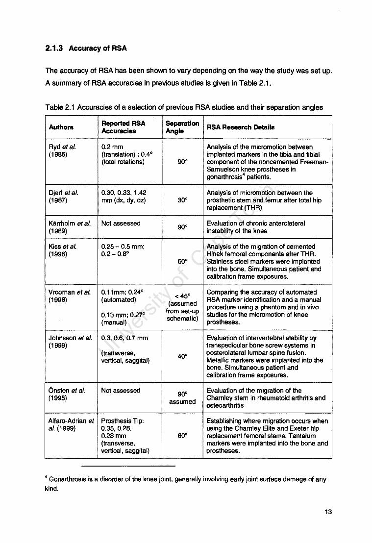
The accuracy of RSA has been shown to vary depending on the way the study was set up.
A summary of RSA accuracies in previous studies is given in Table 2.1.
Table 2.1 Accuracies of a selection of previous RSA studies and their separation angles
Authors Reported RSA Separation RSA Research Details Accuracies Angie
Ryd etal. 0.2mm Analysis of the micromotion between (1986) (translation) ; 0.4° implanted markers in the tibia and tibial
(total rotations) 90" component of the noncemented Freeman-Samuelson knee prostheses in gonarthrosis4 patients.
Djerf etal. 0.30, 0.33, 1.42 Analysis of micromotion between the (1987) mm (dx, dy, dz) 30" prosthetic stem and femur after total hip
replacement (THR)
Karrholm et al. Not assessed 90" Evaluation of chronic anterolateral (1989) instability of the knee
Kiss et al. 0.25 - 0.5 mm; Analysis of the migration of cemented (1996) 0.2-0.8° Hinek femoral components after THR.
60° Stainless steel markers were implanted into the bone. Simultaneous patient and calibration frame exposures.
Vrooman et al. 0.11 mm; 0.24° <45"
Comparing the accuracy of automated (1998) ( automated) (assumed RSA marker identification and a manual
procedure using a phantom and in vivo 0.13 mm; 0.27" from set-up studies for the micromotion of knee (manual) schematic) prostheses.
Johnsson et al. 0.3,0.6,0.7 mm Evaluation of intervertebral stability by (1999) transpedicular bone screw systems in
(transverse, 40" posterolateral lumbar spine fusion. vertical, saggital) Metallic markers were implanted into the
bone. Simultaneous patient and calibration frame exposures.
Dnsten et al. Not assessed 90° Evaluation of the migration of the (1995) assumed Charnley stem in rheumatoid arthritis and
osteoarthritiS
Alfaro-Adrian et Prosthesis Tip: Establishing where migration occurs when al. (1999) 0.35,0.28, using the Charnley Elite and Exeter hip
0.28mm 60" replacement femoral stems. Tantalum (transverse, markers were implanted into the bone and vertical, saggital) prostheses.
4 Gonarthrosis is a disorder of the knee joint, generally involving early joint surface damage of any kind.
13

Accuracy could either be determined from the standard deviation of a series of
measurements or by using a test object (Kiss et al., 1996). The original study found an
RSA accuracy of 0.03 - 0.05 mm for translations and 0.2° for rotations (Selvik, 1989). One
must bear in mind that the accuracies cannot be compared directly since slight differences
in apparatus and approach may affect the overall accuracy of the study. One such variable
is the separation angle, the angle between the X-ray beams at their point of intersection,
also called the X-ray tube convergence angle. The studies reviewed used a separation
angle of between 30° (Ojerf et al., 1987) and 90° (Ryd et al., 1986).
The studies of Yuan and Ryd (2000) have shown that a higher marker reconstruction
accuracy can be obtained using an interpolation cage (object markers inside the
calibration volume) as opposed to extrapolation (object markers outside the calibration
volume). This result agrees with the camera photogrammetry field research findings that
have shown large extrapolation errors when markers outside a calibration volume are
reconstructed (Wood and Marshall, 1986; Gazzani, 1993; Yuan and Ryd, 2000). Certain
applications require unrestricted space, e.g. gait analysis, and therefore extrapolation is
still used even though it has been shown to be less accurate (Wood and Marshall, 1986;
Choo and Oxland, 2003). In addition, an improvement in accuracy is reported when
greater numbers of control points are used, although accuracy improvement approaches
an asymptote when the number of control points exceeds twenty-one (Yuan and Ryd,
2000).
Since RSA has been used for several decades, various improvements have been made
that have resulted in a more user friendly and less time consuming approach. In the early
literature, the X-ray films were measured by cartographers and microcomputers were used
to calculate the 30 coordinates (Ryd et al., 1986; Karrholm et al., 1989). As technology
progressed, the X-ray images could be digitised using a electromagnetic digitising tablet
(Kiss et al., 1996) or CCO camera linked to a computer (Wang et al., 1996) so that image
processing could be used to automate the marker identification process. In the most
recent literature, digital X-ray images and image processing techniques were used to
perform the RSA (Vrooman et al., 1998; RSA Biomedical Website, 2006).
14
2.2 Direct Linear Transformation (DL T)
2.2.1 Overview
Abdel-Aziz and Karara (1971) originally developed the Direct Linear Transformation (DL T),
which represents a projective transformation between the object space and the image
plane and allows spatial coordinate reconstruction from two-dimensional images (Adams,
1981). The DL T algorithm is frequently used for three dimensional reconstruction of points
from calibrated two-dimensional images in camera and video photogrammetry applications
(Chen et al., 1994; Ras et al., 1996; Meintjes et al., 2002; Douglas et al., 2003). Like the
RSA method, the DL T plays a significant role in biomechanics for reconstruction in stereo
photogrammetric systems (Challis and Kerwin, 1992; Hinrichs and McLean, 1995;
Kofman, et al., 1998). Choo and Oxland (2003) presented a comparison between the DL T
method and the fiducial control plane (RSA) method and concluded that DL T analysis
could be used to enhance the accuracy of traditional extrapolation sterophotogrammetry.
2.2.2 DL T Algorithm
During calibration, the DL T equations are used to calculate eleven transformation
parameters (81 - 811) for each image. These parameters describe the relationship
between two and three dimensions. Using these parameters and the image coordinates of
unknown points, the spatial coordinates of the unknown points can be found.
Figure 2.4 below illustrates the 'co-linearity condition'. This means that since a standard
X-ray image is formed by the projection of an object on the image plane, a point on an
object, M, and its corresponding point on an image, P, and the projection centre node,
X-ray source S are in a straight line (collinear). This intuitive condition is very important as
it leads to the development of vector relationships that allow us to define the eleven DL T
parameters. These parameters are in fact a description of the relationship between the
object space reference frame and the image plane reference frame (Mitton et al., 2000;
Kwon website, 2006).
15
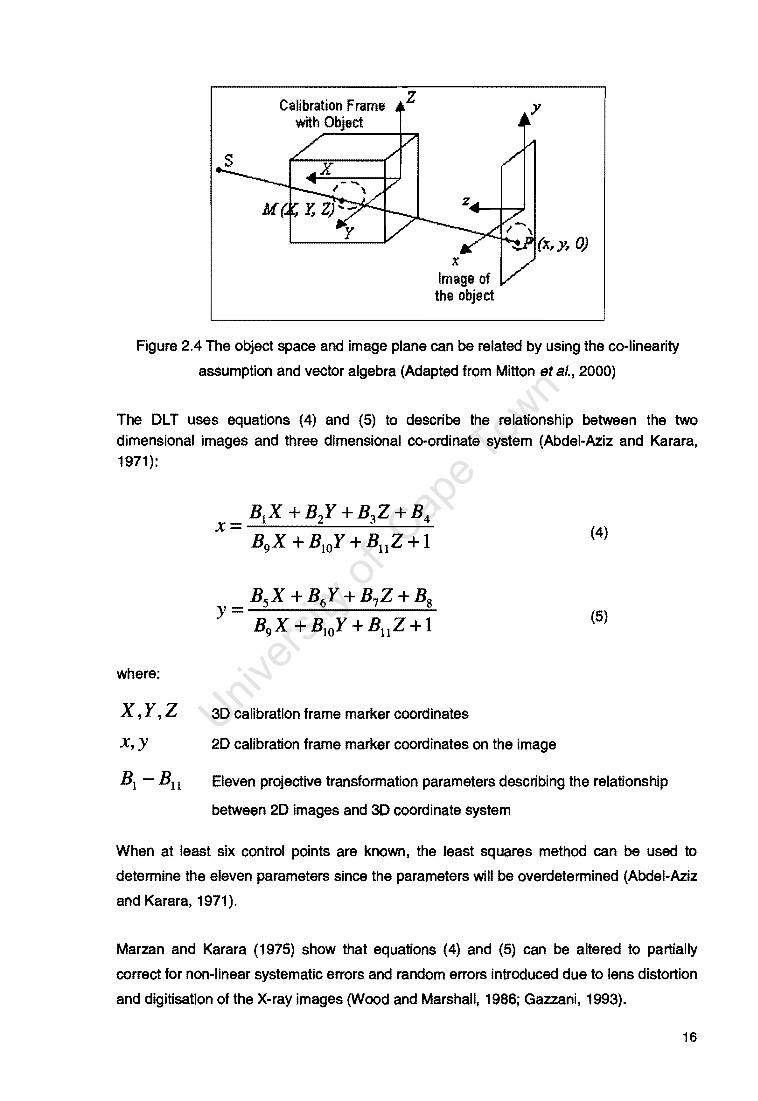
Calibration Frame with Object
z
x Image of the object
Figure 2.4 The object space and image plane can be related by using the co-linearity
assumption and vector algebra (Adapted from Mitton et al., 2000)
The OLT uses equations (4) and (5) to describe the relationship between the two
dimensional images and three dimensional co-ordinate system (Abdel-Aziz and Karara, 1971):
where:
X,Y,Z
X,Y
B1X +B2Y +B3Z +B4 X = --=----=---....;:;....--...;...
B9 X + BlOY + BllZ + 1 (4)
B5 X +B6Y +B7Z +Bg Y = -.;;;.---"-------'---..;;.. B9 X + BlOY + BllZ + 1
(5)
30 calibration frame marker coordinates
20 calibration frame marker coordinates on the image
Eleven projective transformation parameters describing the relationship
between 20 images and 30 coordinate system
When at least six control pOints are known, the least squares method can be used to
determine the eleven parameters since the parameters will be overdetermined (Abdel-Aziz
and Karara, 1971).
Marzan and Karara (1975) show that equations (4) and (5) can be altered to partially
correct for non-linear systematic errors and random errors introduced due to lens distortion
and digitisation of the X-ray images (Wood and Marshall, 1986; Gazzani, 1993).
16

The DL T differs from the RSA method in that it does not assume separate planar
calibration markers, instead it uses all the markers simultaneously to calculate the
calibration parameters (Abdel-Aziz and Karara, 1971; Choo and Oxland, 2003). The
advantages, listed by Challis and Kerwin (1992), of the DL T are that (a) the optical axes of
the cameras do not need to intersect; (b) the camera positions can be arbitrary; (c) only
two camera images are required; and (d) additional cameras can be accommodated.
These advantages are also valid for the RSA reconstruction algorithm.
2.2.3 The DL T calibration frame
As with the calibration for the RSA method, the DL T calibration frame depends on the
intended application, as well as whether the DL T will be performed using extrapolation or
interpolation. A few examples of calibration frames discussed in the literature are
described here.
In order to assess the 3D structure of the human spine by radiographic DLT interpolation,
Andre et al. (1994) used a calibration frame made from three parallel equidistant acrylic
plates, each plate having 21 steel balls (calibration markers) embedded in the acrylic. The
steel balls were 0.7 mm in diameter and the coordinates of the calibration markers were
measured using a vertical vernier (Andre et al., 1994). In another lumbar spine study.
Plamondon and Gagnon (1991) describe a calibration frame (30 cm x 30 em x 20 cm)
using 153 metallic balls 1 mm in diameter, however only 30 of these balls were used for
calibration purposes at anyone time. In this study, the calibration frame was rotated
instead of the X-ray source.
Wood and Marshall (1986) performed a DL T study in extrapolation using conventional
cameras to assess a sprinter's stride. The large calibration cage was made from square
aluminium tubing (3.5 m x 2.5 m x 1.5 m) with forty three calibration markers painted onto
the structure. Close-range photogrammetric techniques were used to calibrate the
coordinates of each marker to an accuracy (mean error over X, Y and Z) better than
±1 mm. In another conventional camera DL T study of stride, Hatze (1988) also used a
large calibration frame (0.4 m x 2 m x 2 m) with thirty 40 mm square markers.
To assess the accuracy of the DLT method and its sensitivity to number of control points
and control point distribution in conventional stereophotogrammetry, Chen et al. (1994)
used a rectangular (2.10 m x 1.35 m x 1.00 m) calibration frame with 32 control markers
17
(3M retroreflective tape). Each marker was 3.16 cm in diameter and the marker locations
were established with a transit theodolite to an accuracy of 0.5 mm.
In a conventional cinematography study to compare the accuracy of the DL T with and
without extrapolation, Hinrichs and McLean (1995) used large spherical markers (3 cm
diameter) that were hung on strings from a ceiling (4 markers on each of the 27 strings).
The positions of the markers were found using triangulation, sliding callipers and a transit
theodolite to an accuracy of 0.5 mm.
In a study to determine the effect of control point configuration on DL T reconstruction
accuracy, Challis and Kerwin (1992) evaluated results using a 1.0 m x 0.6 m x 1.0 m
calibration frame that incorporated five different configurations. By selecting specific
points, the frame was changed from one where control points encompassed the whole
volume of interest ("Christmas tree" configuration) to where control points were distributed
around the outside of the volume of interest. The markers were fifty 42 mm diameter
spheres that were centrally drilled to fit on steel tubing. The markers were colour coded
according to the different configurations. Since this was a camera photogrammetry study,
there was no concern regarding the X-ray characteristics of the material. The marker
locations were determined using a laser-based surveying system to an accuracy of
±0.8mm.
In order to compare the RSA and DLT reconstruction techniques, Choo and Oxland (2003)
used several different calibration cages, one for extrapolation and several interpolation
cages. The reference markers used were 3 mm in diameter.
2.2.4 The DL T calibration process
In order to solve for the eleven DL T parameters (see equations 4 and 5) of each X-ray
source poSition, a minimum of twelve equations is needed. This means that we need at
least six control points with known X, Y and Z coordinates in very good 3D spatial
distribution, along with the corresponding (x, y) image coordinates of those points (Chen,
1994; Mitton at al., 2000), since each control point provides two equations. The system is
then overdetermined since there are more equations than unknowns. To compute the DL T
parameters, a linear least squares method could be used (Hatze, 1988). The method of
least squares is a common method for solving overdetermined systems of equations (Zill
and Cullen, 1992).
18

The two sets of eleven OLT parameters. one set for position 1 or left X-ray source position
(Bu - BU1 ) and one set for position 2 or right X-ray source position (BA1 - BA11 ), are used
together with the image points from the left image (XL. YL ) and the right image ('<A, YA) to
calculate the 3D coordinates of a point (X,Y,Z) within the calibrated volume. Once the
transformation parameters have been obtained, the X-ray source-detector configurations
must not be disturbed to ensure that no further errors are introduced.
2.2.5 Accuracy of the DLT
Like the RSA method, the OL T accuracy reported in journal papers varies. One must also
bear in mind that the axes (X, Y, Z) used are often labelled differently in each study. It
must also be noted that the apparent accuracy given when pOints that were used in the
development of the transformation parameters (control points) are reconstructed can be
misleading. True reconstruction accuracy should be assessed by the reconstruction of
non-control (test) pOints (ChalliS and Kerwin, 1992). Transformation errors from a selection
of previous OL T studies are summarised in Table 2.2.
Table 2.2 Three dimensional error of a selection of previous OL T studies. CJ = standard
deviation; RMS = root mean square.
Author Transformation Separation
Application Error Angle(a)
Andre (1994) 15.0 mm (using Vertical stereo-radiography for the vertebral landmarks) clinical 3D reconstruction of the
30° spine.
1.0 mm (using implanted steel ball markers.)
Wood and 5.7 mm (best result Conventional camera stereo-Marshall (1986) from all experiments)
45° and 90° photogrammetry using extrapolation to assess a sprinter's stride. Control points have been reconstructed.
Hatze (1988) 4.7 - 5.2 mm (mean Conventional camera stereo-RMS errors for 30 - 7 59° photogrammetry comparing the DL T control points using and a modified DL Tusing DLT) reconstruction of control points
Dansereau and 0.72 mm (0 of The development of a method to Stokes (1988) measurement errors) measure the 3D shape of the rib
20° cage to provide descriptive data and to study symmetry in the normal population.
Plamondon and 0.2 mm (mean 15° - 90° (in Assessing the effect of configuration
Gagnon (1991) accuracy. each axis) intervals of
of data acquisition on the accuracy
15°). 105° of stereo-radiographic system for an
and 1200 application in lumbar spine motion studies.
19
Author Transformation Separation Application Error Angle(s) Chen etal. 6 -7 mm (resultant Conventional camera stereo-(1994) errors)
35° photogrammetry studying the effect of number and distribution of control points.
Hinrichs and mean = 0.61 mm, Conventional cinematography using McLean (1995) C1 =0.14 mm; the standard DL T and extrapolation
extrapolation: 90° DLT. mean = 6.01 mm, C1 =1.42 mm
Stefansic et al. 0.7 ± 0.2 mm (11 N/A Mapping 3D patient space to
(2000) control points used) (mapping is laparoscopic (endoscopic) image
from 3D to space using the DL T and in
single2D minimally invasive hepatic surgery. Different numbers of control points image) were assessed.
Chooand 0.33 mm (control A study showing improved RSA Oxland (2003) point calculation in accuracy when including DL T and
simulations) balanced marker distribution. 20"
0.23 mm (test point reconstruction in phantom study)
Challis and 4.3 - 5.5 mm RMS Study of the DL T accuracy for the Kerwin (1992) error for non-control
85° reconstruction of control points and
points (11 control test points with different control point points) Quantities and configurations.
Andre et al., 1994 reports three dimensional error (differences between the measured and
reconstructed marker coordinates) of under 1.0 mm when using steel balls as markers.
The error increased to as much as 15.0 mm when using vertebral landmarks since they
were not as clearly visible on the X-ray images (Andre et al., 1994), see Table 2.2. This
highlights the importance of accurate identification of the markers on the X-ray images.
The calibration marker coordinates should also be measured with a high degree of
accuracy in order to reduce the reconstruction errors (Andre et al., 1994).
Wood and Marshal (1986) investigated the accuracy of the DL T -extrapolation method in a
conventional camera stereophotogrammetric assessment employing several different
experiment configurations. It was found that there are Significant reconstruction errors
when using extrapolation. The best results were achieved in the experiment with the
highest number of control points (30) and the greatest distance:base rati05 between
camera positions. The average RMS error for this best situation was 5.7 mm.
5 This ratio describes the orientation of the cameras and is interpreted to correspond to the separation angle discussed in similar studies.
20
As in RSA, an improvement in accuracy is observed when increased numbers of control
points are used for the OL T, however this improvement has been shown to be limited
when more than 16 control points are used (Chen et a/., 1994): the resultant mean
absolute error and resultant standard deviations were 14.6 mm and 19.5 mm when eight
control points were used, 6.6 mm and 3.0 mm when sixteen control points were used, and
7.1 mm and 3.4 mm when twenty-four control points were used. The Chen et a/. (1994)
study also reinforces the importance of using well-distributed control points around the
volume, especially when few control points are used and emphasises that extrapolation
should be avoided where possible.
Hinrichs and McLean (1995) also compared the accuracy of the standard OLT and
extrapolated OLT and the results agreed with Wood and Marshal (1986) and Chen et a/.
(1994) in that higher errors are to be expected when using extrapolation.
The study by Plamondon and Gagnon (1991) addressed whether the configuration of data
acquisition in radiography has an effect on the accuracy of three-dimensional
reconstruction using the OL T. The accuracy of 3D reconstruction was found by
reconstructing twenty known points on the calibration frame that were not used in the
generation of transformation parameters. The error was taken as the absolute difference
between the calculated coordinate and the measured coordinate value. The results
showed that as the separation angle was increased, the accuracy in the Z-axis (defined as
the axis between the film and the X-ray source for one exposure) increased. The mean
accuracy for each axis (X, Y, Z) was less than 0.2 mm for all stereograms and the
maximum error was 0.39 mm in the Z direction when a separation angle of 30° was used.
The modified OLT (MOLT) was developed by Hatze (1988) in an attempt to improve the
accuracy of the three-dimensional object space reconstruction. Linear and non-linear
algorithms were presented however there are certain conditions that must· be satisfied
since the MOLT reduces the number of OLT parameters needed. The linear algorithm
requires at least 15 evenly distributed control points, and the non-linear algorithm requires
more than 30 evenly distributed control pOints (Hatze, 1988).
The MOLT makes use of the fact that the eleven parameters of the standard OL Tare
made up of only ten independent unknown parameters. The MOLT works to eliminate the
redundant parameter by expressing one parameter in terms of the others.
21

The MOLT has only ten parameters since it assumes that the x and y axes in the image
space are perpendicular. With the MOLT, theoretically only 5 known control pOints are
needed, but an increased number increases reliability with the increased redundancy. A
reconstruction accuracy of 0.733 mm RMS mean error was reported when reconstructing
control points in the original study using the non-linear MOLT (Hatze, 1988).
In a computer simulation, Gazzani (1993) compared the extrapolation OL T method to a
method he called CESNO (Collinearity Equation Solution by Numerical Optimisation),
which is similar to the MOLT, for an application in conventional camera
stereophotogrammetry. The separation angle of the simulated cameras was 60°. The
minimum number of control points for reasonable accuracy when using the linear OL Twas
given as 12 control points, while between 12 and 16 control points are needed when using
the MOLT I CESNO.
2.3 A Two-Dimensional Projective Transformation Method
2.3.1 Overview
Adams (1981) published a method for three dimensional localisation of image points in
stereo X-ray images using three-dimensional projective transformation algorithms. The
proposed system did away with the requirement to perform the studies under ideal
conditions so that stereophotogrammetry could be performed with the use of apparatus
normally available in a clinical environment (Adams, 1981).
Based on the Adams method, van Geems et al., (1995) devised a two-dimensional
projective transformation resembling the OL T for the calculation of three-dimensional
computed tomography (CT) coordinates of image pOints from CT scan projection
radiographs (SPRs). A variety of names have been given to SPRs including: ScoutView™,
Pilot Scan™, Surview™, Topogram™, Scanoscope™, Scanogram, radiographic mode and
localizer image (Medcyclopaedia website, 2006).
An SPR is a series of image lines obtained along the body's vertical axis in a CT system
(the Z axis) to make up one image. The X-ray beam producing each image line projects
outwards in the XV-plane, where the X direction is along the body's anterior-posterior axis
and the V direction is along the body's lateral axis, similarly to the Statscan X-ray beam.
This method was initially applied to anterior-posterior and lateral SPR views (van Geems,
1996).
22

The equations used relate SPR coordinates to CT slice coordinates. The x-coordinates of
a point in two two-dimensional SPR lines determine the X- and Y coordinates of the
corresponding point in the three-dimensional CT image. The y-coordinate of the SPR is
linearly related to the Z-coordinate in the CT image.
2.3.2 The Projective Transformation Algorithm
The algorithm details can be found in Section 3.2 since this method was used with
Statscan images to locate the three-dimensional coordinates of markers.
2.3.3 Calibration for the Projective Transformation
Van Geems (1997) made use of 16 well distributed control markers with known three
dimensional coordinates for calibration. The method requires a minimum of six control
markers. The coordinates were measured using a metrograph6 with a measuring
resolution of 0.1 mm on each axis.
2.3.4 Accuracy using the Projective Transformation
The accuracy of the study performed by van Geems (1997) is given by the mean error and
the standard deviation of the difference between reconstructed points using the SPR and
actual CT slice coordinates as shown in Table 2.3.
Table 2.3 Comparison of CT slice coordinates and those calculated from the SPRs
dX dY dZ
Mean Error (mm) -0.9 0.3 1.4
Standard Deviation (mm) 0.5 0.5 0.6
For comparison, the study by Aubin et a/. (1997) reported an accuracy for CT-scan 3D
reconstructions being approximately 1.1 ± 0.8 mm. The accuracy of the X and Y
coordinates were therefore within the typical accuracy of a CT scanner.
6 Instrument tor line-ot-sight three dimensional measuring
23

2.4 The Non-stereo Corresponding Point Method (NSCP)
2.4.1 Overview
This method, presented by Mitton et al. (2000), shows an improvement on the DLT
procedure for three-dimensional reconstruction of X-ray images of dry cervical vertebrae.
The method uses two-dimensional points identified in one X-ray image only, deformable
meshes with simulated springs and the principle that any non-stereo corresponding point
belongs to a line joining the X-ray source and the projection of the pOint in one view. This
has been called the non-stereo corresponding point (NSCP) method. A validation of the
NSCP three-dimensional reconstruction technique for lumbar vertebrae was performed by
Mitulescu et al. (2001) by comparing four techniques: direct measurement, CT scan, the
DL T and the NSCP method.
In addition to the corresponding points, this method also makes use of points that are not
clearly defined on a stereo-pair of images and could therefore be employed when
anatomical landmarks are reconstructed. This may be useful since the studies of both
Dansereau (1988) and Andre (1994) mention that it is difficult to identify corresponding
pOints when using anatomical landmarks.
2.4.2 The NSCP algorithm
The NSCP algorithm method consists of first performing the DL T (Abdel-Aziz and Karara,
1971; Marzan and Karara, 1975) in order to reconstruct the corresponding points on two
X-ray images. The NSCP technique is then used to reconstruct the non-corresponding
points (Mitton et al. , 2000). If a point is clear on one image, but not clear on the other, the
only information that can be used for reconstruction is that the 3D position is on a straight
line (named the constraint line) between the X-ray source and the single 2D image point.
To enable reconstruction of this point, assumptions need to be made about the geometry
of the object to be reconstructed (Mitton et al., 2000). A generic object is defined using the
constraint lines and 3D points obtained from the DL T as geometrical constraints. The
position of the non-stereo corresponding point on the constraint line is found by elastically
deforming the generic object while respecting the defined geometrical boundaries. In order
to get the mesh as close as possible to the generic object, deformation energy is
calculated using Hooke's law (Mitton et al., 2000):
24
where:
10k
1" K
initial length of the J(h spring in the generic object
actual length of the. J(h spring in the generic object
the spring constant (stiffness)
2.4.3 Accuracy of the NSCP method
(6)
The NSCP reconstruction technique has reported mean errors of 1.1 mm with a maximum
error of 7.8 mm compared to direct measurements (Mitulescu et al., 2001). The drawback
of this method is that the generic object has to be well defined based on previous
knowledge about the object to be radiographed.
2.5 Image Marker Identification used in Previous Studies
Accurate identification of the two-dimensional coordinates from a pair of stereo X-ray
images is vital to ensure good reconstruction of the three dimensional point position. This
section reviews the literature on the use of digital image processing of X-ray images, with
a focus on marker centroid7 identification.
2.5.1 Identifying the two-dimensional marker positions
One of the challenges in X-ray stereophotogrammetry is the identification of markers on
the X-ray images since the marker positions may be distorted and it could be difficult to
identify the corresponding points on two separate images (Nystrom et al., 1994). In a
conventional camera stereophotogrammetry study. van der Vlugt (1991) investigated a
marker matching technique to match the appearance of an object on one image with it's
appearance on another two images, however this approach was not used in the final
program since some markers appeared on two, but not three images. instead, a
combination of automatic and computer aided manual techniques were used to identify the
markers on each image (van der Vlugt, 1991).
7 Centre of gravity of an object
25
User intervention, together with careful calibration frame design was required in most
studies to simplify the identification of the stereo-pairs. The user had to be familiar with the
calibration frame and marker numbering in order to identify the same marker on each
image since the markers were first identified by means of a mouse and cursor (Ostgaard
et al., 1997).
Vrooman et al. (1998) used pixel thresholding and Sobel digital edge enhancement
followed by a circle finding technique on raw digitised X-ray images (150 dpi, 8-bit
resolution) in order to identify the markers in an RSA study on total knee prosthesis
micromotion. The different types of markers, which were labelled prosthetic, bone and
calibration markers, had different diameters and could therefore easily be identified by
altering the diameter used in the circle finding algorithm. The technique relied on the
known distribution and pattern of the calibration markers in order to label them correctly.
The bone and prostheses markers were then matched using projection lines. The program
allowed for the marker labelling to be checked and corrected by the user if it was incorrect.
2.5.2 Locating the Marker Centroid
Prior to using digital means to locate the marker centroid in RSA studies, the location was
typically done using a measuring table (Ostgaard et al., 1997). Ostgaard et IU. (1997),
assessed the accuracy and reproducibility of marker centroid positions using digital image
processing algorithms and digitised X-rays with a resolution of 600 dpi and 256 grey
levels. A 30 X 30 pixel area around the marker, which was identified by the user using a
mouse and cursor, was used as a region of interest. The image was first smoothed using
an averaging filter and then the region of interest was binarised using the threshold values
determined by the mean of the minimum and maximum grey-scale values. The edge of the
marker was detected by contour analysis; using the edge of the marker, the centre was
found by a linear approximation of the circle equation (Ostgaard et al., 1997).
Using a computer and digitised images proved advantageous in that it was easier to
identify the markers on the PC monitor; however, a disadvantage was that the digitisation
of the films limited the resolution (Ostgaard et al., 1997). This is not a problem in the
current study since the X-ray images are already digital and the user has an option of high
or low resolution when scanning.
Wang et al. (1996) provided an optimised method for locating reference markers on
orthopaedic X-ray images. This was for the purpose of performing RSA effectively and
26
with high accuracy. The reference markers were implanted during surgery. X-ray films
were digitised and non-linear image processing algorithms based on mathematical
morphology, e.g. erosion and dilation, were used to find the markers. For the marker
centre, a grey-scale weighting function was used.
In a conventional camera stereophotogrammetry study, van der Vlugt (1991) used a
threshold technique to convert the images to binary images in order to separate the
markers from the background. The technique converts all the pixel intensity values above
a suitable threshold value to 225 (white) and all below to 0 (black). The program used an
input look up table (ILUT) and user inspection to threshold the image (van der Vlugt,
1991). Using the thresholded image and edge detection, the edges of the markers were
identified. USing this information and the original grey image to ensure that all information
was used, a weighted centre of gravity method was used to determine the marker centres.
If the marker area was found to be larger or smaller than a preset value, then it was
discarded as a non-marker (van der Vlugt, 1991).
In another conventional camera stereophotogrammetry study, Rogus ~t al. (1999)
designed a system to reduce patient positioning errors for radiation therapy. The standard
thresholding and centroid calculations that were employed did not include size, shape or
location constraints such as .that used by van der Vlugt (1991), and therefore any non
marker reflective objects had to be covered to prevent the false identification of such
objects as markers (Rogus et al., 1999). The markers were often seen as ovals since the
camera viewed the circular markers from an angle (Rogus et al., 1999).
Lam et al. (1993) developed algorithms to automatically locate markers on digitised X-ray
images for use in radiation therapy patient positioning. The first algorithm was used to
locate marker pOSitions on a pair of X-ray images by linear filtering where image features
with a circular component were enhanced and those without were suppressed. Grey scale
thresholding was then performed where non-marker features were suppressed to form a
binary image and finally, potential marker regions that were too large or too small to be
markers were rejected (Lam et al., 1993).
The second algorithm located marker pOSitions on a pair of X-ray images by comparing
them to a reference pair obtained in the first patient examination. By exploiting information
from the reference images such as marker shape, size, contrast and locations, marker
identification could be done automatically and the algorithm only needed to search small
regions around the reference marker position (Lam et al., 1993).
27
Vrooman et al. (1998) fitted a paraboloid to the grey scale value of the markers in order to
find the centroid.
More advanced digital methods of calculating the two-dimensional marker position using
mathematical models have been described by Borlin 1997 and Borlin et aI., 2002;
however, these are not investigated in detail in this project.
2.6 X-Ray Stereophotogrammetric Applications
This section reviews applications of X-ray stereophotogrammetry in the field of medicine.
A summary of the use of photogrammetry in medicine, not specific to X-ray
photogrammetry can be found in the literature by Mitchell and Newton (2002).
2.6.1 Migration Assessment
RSA is widely used in the field of orthopaedics and biomechanics, especially in the
assessment of the migration of prosthetiCS and joint stability since the method allows the
rotations and translations of skeletal segment movements to be determined (Selvik, 1989).
The technique can measure the migration and rotation of prostheses relative to bone in
tenths of millimetres and degrees (Kiss et al., 1996).
Conventional X-rays can detect a certain degree of micromotion of prostheses, but are
limited to measurements of the acetabular region and can only measure in one plane
(Nilsson and Karrholm, 1996). Routine X-ray images can be used to detect movement of
approximately 5 mm (Nilsson and Karrholm, 1996), which is not sufficient accuracy to
assess the success of the surgery since the prosthesis shUt that must be detected is much
smaller than this.
Much of the literature reviewed involves the analysis of hip prosthesis stability. RSA is
used to measure the movement of an implant relative to bone in three dimensions to an
acceptable degree of accuracy (Cnsten et al., 1995; Nilsson and Karrholm, 1996; Alfaro
Adrian et al., 1999; Valstar et al., 2002). To enable an assessment of the success of hip
replacement surgery, it is advantageous to determine any movements between femur and
prosthesis shortly after the operation (Ojerf et al., 1987). RSA has the potential to predict
implant performance as soon as possible after implantation, which means that the success
of a new prosthesis can be analysed without the patient suffering through the usual clinical
28
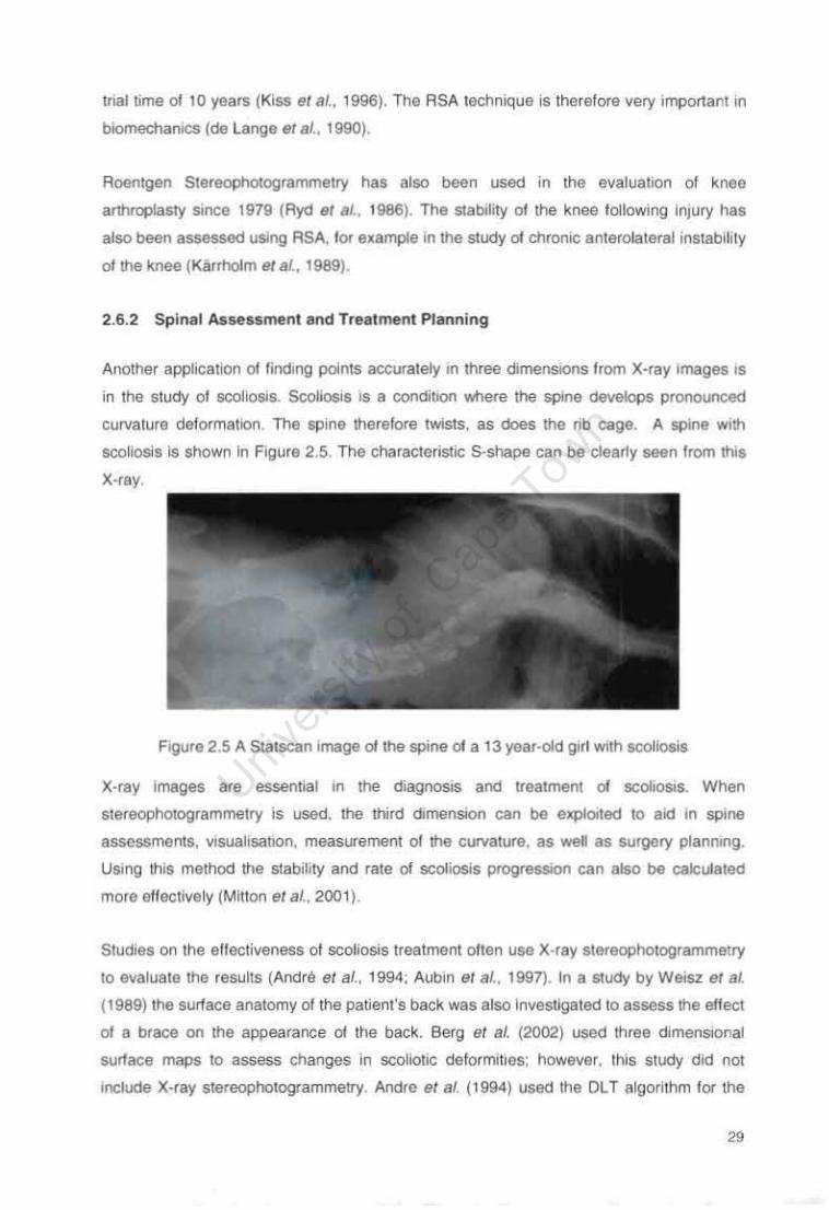
trial lime of 10 years (Kiss el 81" 1996), The RSA technique Is therefore very Important In
blOll'leChanics (de Lange Sf al" 1990).
Roentgen Siereophologrammelry has also been used in the evaluation of knee
arthroplasty smce 1979 (Ryd SI ., .. 1986). The stabihty of the knee loIlowing Injury has
also been assessed using RSA, lor example In the study 01 chronIC anteroiateraJ instability
of the knee (Kirrllolm Bf sl .. 1989).
2.6.2 Spinal Anenmentand Treatment Planning
Another applICation oI l indmg points accurately In three dimefISIOfIs from X-ray Images IS
in the Study of scol~Sls. ScolIosis is II condi\JOfl wnere the spine develops pronounced
curvature deformaHon The spine therefore twists. as does the rib cage. A spine With
scoliosis Is shown In Figure 2.5. The characteristIC 5-shape can be clearly seen from this
X-ray.
Figule 2.5 A Statscan Image oI lhe spine 01 a 13 year·oId glfl with scoliosis
X·ray Images are essential In the diagOOSlS and treatment 01 scoliosis. When
Slereophoiogrammetry Is used, the third dimenSion can be explorted 10 aid In spine
assessments, Vlsuali&atlon, measuremem 01 the curvature, as weI as surljlOry plannlflg.
USing this melhod the stability and rale 01 scoliosis progression can also be calculaled
more elf8(:tively (Minon ef al .• 2001) .
Studies on the eliactiveness 01 scoliosis treatment ollen use X·ray stereophologrammetry
to evaluate the results (Andre et al., 1994; Aubm et al. , 1997), In a study by Weisz el ai,
(1989) the SUrlace anatomy of the patien!"s back was also Invesllgatecllo assess the effect
01 a brace on the appearance 01 the back. Berg sr al. (2002) used three d,menSiOflat
surlace maps to assess changes In scoliotiC deformities: however. thiS Study did not
Include X-ray stereophotogrammetry. Aadre et al. (1994) used the OLT algorithm for the
"
three-d imensional recorostructlon 01 the human spine The DL T can be performed on
pati"nt .. in an up, iOI'T pOSiT .. ,..., lInrl is th"r"fm" r.omfl"lIhle WITh rli"[JnMlir. flmIOC()I ~ Inr
scol iOSis diagnoSIS {Mitton el al" 20(0).
The IntelVertebral stability of transpedicu lar fixation lumbar fusion 01 the spine has been
evaluated In previous studies With high accuracy using Ihe RSA method. RSA provides a
safe radiographiC method for assessing fixati oo Without the intrUSive surgery reQUifed lor
fUSion exploration (Johnsson el al., 1 999).
2.6.3 Radiat ion Oncology
Tho 3D local isation 01 pOints from Images has applications In rad iation oncology such as
brach)'lherapy, the Implantation of rad ioactIve seeds to Ireal cancer. (Jackson. 1983:
Siddoo and Chin, t985; Lam and Ten Haken, 1991), A post·implant evaluation is
necessary to evaluate the source placement errors so thaI the Impact on the coverage 01
the volume of Interest can be established {Martel and Narayana. t998).
The pOSitioning 01 pallents for rad iation therapy is another appllcahon in the Irealmen! of
cancer. Accurate pallent positioning in retation 10 tllO treatment machine and thus the
rad,alion beam is very Imponant in conformal radlahon therapy such as proton therapy
becausa of the small margins used (Rogus e/ al" 1999). In conformal (adlallon therapy.
the radiation beam is shaped in th ree-dimensions so that the radiat loo dose to the larget
volume IS maXimised while the dose to the surrounding normal tissue lS mimmised (Martel
and Narayana, 1998).
2.6.4 Cephalometry
The use of X·rays to determine the three dimenSional measurements 01 craniofaCial
landmarks was first introduced by Broadbent (1931) and a vanely 01 methods have smee
been developed with applications In the fields of dentistI)'. orthodont.cs and maxillotacial
surgery (Papadopoulos el al" 2(02) It is of photogrammetriC mterestlhal1n several facia l
studies. X- ray techmques have been used together With camera photogrammetry (Mitchell
and Newton, 2002) There IS also scope for the use of X-ray slereophotogrammelry In
cranium growth assessments (Albenus el al .. 1990).

2.6.5 Additional Applications
Additional appIielltionS lor X-ray stereophotogrammetry exist. such as assessing !racrure
stability al'ld joint kInematics. where joint stability can be assessed (Kafl'hoim 61 al.. t999)
and Where the stabil~y 01 ligaments (e.g. anterior cruciale ligament) IS determined. There
is also scope lor the use 01 X-ray stereophotogrammetry in computer aSSISted surgery
(MIlton or al" 2000: Vals!ar or al •• 2002). In addl~on sluclies have even been 00ne USIng
X·ray stereophotogrammetry 101 use In minImally invasive hepatIc surgery (Stefan!t.ic 8/111 ••
2(00).
"

Chapter 3 : Materials and Method
3.1 Statscan Materia ls and Technical Apparatu s
3.1 .1 The Statscan Digital Scanner
Tha Statscan digital scannar (see Figure 3 1) is II tow d05e digital X·ray machine cUrTantly
used for Trauma appl ications at the Groote Schuur Hospita l In Cape Town The scanner is
capable 01 takrng whole body X· ray Images In approximately 13 seconds.
-,
• x
~.
•
• •
Figure 3. ' The Statscan O'g'tal X·ray Scanner with global coordinate system
Statscan performs slot scanning With 12 CCO cameras and produces hlgh·quallty d'g,tal
X-ray Imagas I'I'Th low rad iati on exposure. approximately 2 72% 01 the standard
convenTIonal dose In Trauma applications (Benningfield el al.. 2003). The X-ray source and
d~t"""' r b"n~s ,"" muunl" d "n" C-A"" <ls~rnbly th"t Cdn b" ''''dt~u dround th .. ).Jdl,,,nt
trolley ThiS enables anterror·postenor (0 ) and laleral (90 ) X-ray Images to be raken, as
wel l as ImagBS at any angle between O· and 90 This function ,s essential In Ihls prOject
since it allows lor X·ray images to be taken from diHerent angles without moving !he
pallen t or requiting muillp le X-ray sources. The trolley ,s a 26 mm board made or a Single
piece 01 low density structural toam surrounded by a carbon ',bra sk,n

The Statscan axes have been defined as shown in Figure 3.1 in order to be consistent
with that of van Geems et al., (1995). With the source-detector at a 0° scanning angle with
respect to the patient, the X-axis is vertical, the Z-axis is in the direction of horizontal
C-arm travel and the V-direction is orthogonal to the X-Z plane.
3.1.2 Statscan Digital Radiographs
The digital radiographs are formed from a series of line or slot scans obtained as the
C-arm moves across the patient trolley. The fan-beam projects outward from the source in
two dimensions on the XV plane. The imaging geometry is therefore similar to the fan
beam of computed tomography (Cn rather than the cone of conventional X-ray imaging
as illustrated in Figure 2.2, Section 2.
In fact, in the planning phase of computed tomography, patients often undergo scan
projection radiography (see Section 2.3.1) where the position of the X-ray source is kept at
a fixed angular position with respect to the plane of patient movement in order to localise
the target region. This is effectively what the Statscan scanner achieves.
The Statscan scanner can produce images of an area ranging from 100 mm x 100 mm to
a maximum of 680 mm x 1800 mm. These constraints are important when designing the
calibration equipment (see Section 3.3.1).
The. spatial resolution required can be set before performing an X-ray scan. This can be
either 2.78 Ip/mm on high resolution, or 1.67 Ip/mm on low resolution with 5 x 5 pixel
binning. The fundamental pixel size is 60 ~m. The image pixels are square. The contrast
resolution is 16 000 grey levels. Using the console tools, it is possible to scroll through the
grey levels to improve visibility of structures with differing densities (Benningfield at al.,
2003). The X-ray images can be saved in the DICOM format, however the Bitmap format
was used since it was easier to manipulate in Matlab.
The density of the patient trolley was not taken into account during the image processing
of the images since the density was assumed to be constant throughout and the table
density made a small and insignificant difference to the images. The total attenuation of
X-rays by the table is approximately equivalent to 0.7 mm of aluminium.
33
3.1.3 The Computer Equipment
A Pentium IV processor was used during this project. The operating system used was
Microsoft Windows XP Home. All programming was done in Matlab 6.58• Matlab is very
efficient in running matrix calculations and since images are essentially matrices made up
of pixels, which have different greyscale or colour values, this program was found to be
suitable to perform the processing required.
3.2 Method of X-ray Stereophotogrammetry used with Statscan
The Statscan image acquisition technique is similar to the technique used to obtain scan
projection radiographs (SPRs) for computed tomography (see Section 2.3.1); therefore it
was reasonable to assume that a stereophotogrammetry technique suitable for SPRs
could also be used with Statscan images. The van Geems et al. (1995) method of two
dimensional projective transformation for the calculation of three-dimensional CT
coordinates of image points from CT scan projection radiographs (SPRs) will be used in
this project (see Section 2.3).
3.2.1 Stereophotogrammetry technique suitable for use with SPRs
An important initial observation is that the Statscan Z-coordinate, in the direction of
horizontal C-arm movement, is linearly proportional to the image y-coordinate and
therefore the measurements (in mm) could be obtained from the image coordinates (in
pixels). Since this dimension can easily be derived, we can focus on finding the X and V
coordinates of each "slice".
Using CT terminology one could say that, if calibration markers are known to be on the X
V plane, only one CT slice is required to produce the three-dimensional CT slice marker
co-ordinates. A two-dimensional projective transformation of the x-coordinates from X-ray
images taken at different angles would be sufficient in order to find the X, V coordinates of
each "slice". Following this, the three-dimensional coordinates of the markers could be
established.
In order to determine the transformation parameters, two Statscan images (effectively
SPRs) of the calibration frame must be scanned from different orientations and the
8 The Mathworks, Inc., Natick MA, USA
34

calibration markers must be able to be identified on the images. The equation for the x
coordinate Xk,i of point i on image k is (van Geems et al., 1995):
where the slice coordinates Xi and Yi , and the five h parameters (h k,h •••• h k,s) relate to
image k. The Xk,i value can be found by taking measurements from the X-ray image k and
points Xi and Yi are known from the independent calibration of the calibration frame. These
pOints for each X-ray image are substituted into equation (7).
The five unknown h parameters remain unsolved, thus requiring five non-collinear
calibration markers for a unique solution. If more than five calibration markers are used
this would provide an over-determined system and a least squares method can be used to
solve for the parameters.
Equation (7) can be written in matrix form for calibration markers 1 - n:
Am=L (8)
where:
X) ~ 1 -xk,)X) -Xk,)~ hk,l
X2 Y2 1 -xk,2X2 -Xk,2Y2 hk ,2
A= (f)= hk,3 L=
hk,4
Xn Yn 1 -xk,nXn - Xk,nYn hk ,5
The slice coordinates Xi and Yj of an unknown marker can now be found by back
SUbstitution into equation (7). The coordinate Zi can be determined from the X-ray image
and the slice system. Therefore the three-dimensional coordinates (Xi. Yt• 2() of a point can
be found (van Geems at al., 1995).
3.3 Calibration Equipment
3.3.1 The Calibration Frame Design
A calibration frame or cage is a three-dimensional frame with markers of known
coordinates usually covering the volume of interest. Challis and Kerwin (1992) established
35

that the use of control points around the outside of the volume of interest is preferred to
control points distributed within the volume. The calibration frame is needed to define the
laboratory coordinate system and to find the transformation parameters that will allow
three dimensional coordinates to be found from two-dimensional image coordinates. Once
the volume is calibrated, it will be possible to calculate the spatial coordinates of unknown
markers within the specified space with respect to the defined laboratory coordinate
space.
The accuracy of the transformation depends on the accuracy of the calibration marker
coordinates, and therefore this section of the project was vital. The following had to be
considered during the calibration frame design process:
• The frame had to be rigid and stable with the markers firmly attached so that the
coordinate measurements remain valid.
• The calibration markers had to cover the outside limits of the volume of interest, as
recommended by Challis and Kerwin (1992).
• Theoretically the transformation technique only requires six known calibration
markers or control points; however, studies have demonstrated that reconstruction
accuracy improves with an increased number of control points with limited
improvement when more than 16 control points are used in DL T (Chen et sl.,
1993). The calibration frame therefore had to have at least 16 control points.
The calibration frame had to be calibrated using a line-of-sight camera stereo
photogrammetry technique; therefore the following characteristics were required to ensure
good calibration:
• The markers had to be visible on photographs of the frame taken from many
different angles.
• There had to be sufficient contrast between the markers and the frame structure so
that the markers can be easily identified on the photographs.
• The frame structure material had to be limited so that as few control frame points
as possible were obscured.
• Markers had to be large enough to allow easy identification on the photographs.
36

In addition, the accuracy of calculating the coordinates of unknown markers depends on
the accuracy to which the corresponding coordinates of the markers are located on the
X-ray images. This in turn depends on the image quality, resolution, size of calibration
markers and level of contrast available on the X-ray images. The calibration frame
therefore needed to be optimally designed to enable easy identification of the
corresponding markers on the digital X-ray images:
• The frame material had to be radiolucent and the calibration markers had to be
radio-opaque to provide sufficient contrast between the frame and markers.
• The arrangement of the markers had to be irregular to prevent overlapping markers
on the X-ray images.
• A logical, standardised calibration marker numbering system had to be established
as recommended by Karrholm et a/. (1989).
The dimensions of the possible scanning area also had to be taken into account when
deSigning the calibration frame. The C-arm of the Statscan machine can only be rotated
with the trolley in a raised position and raising the trolley would shrink the maximum
scanning volume available; therefore the trolley height was taken into account. With the
trolley fully raised, the maximum scanning width was 560 mm (see Figure 3.2).
Trolley h~9_ht _ L __ t 1070 mm I (raised)
840 mm 1 (ret r~cted)
X-ray source
Detectors
1 Not to s(;alel
Figure 3.2 The dimensions of the Statscan machine and the height of the trolley limit the
imaging space and provide constraints for the design of the calibration frame.
37
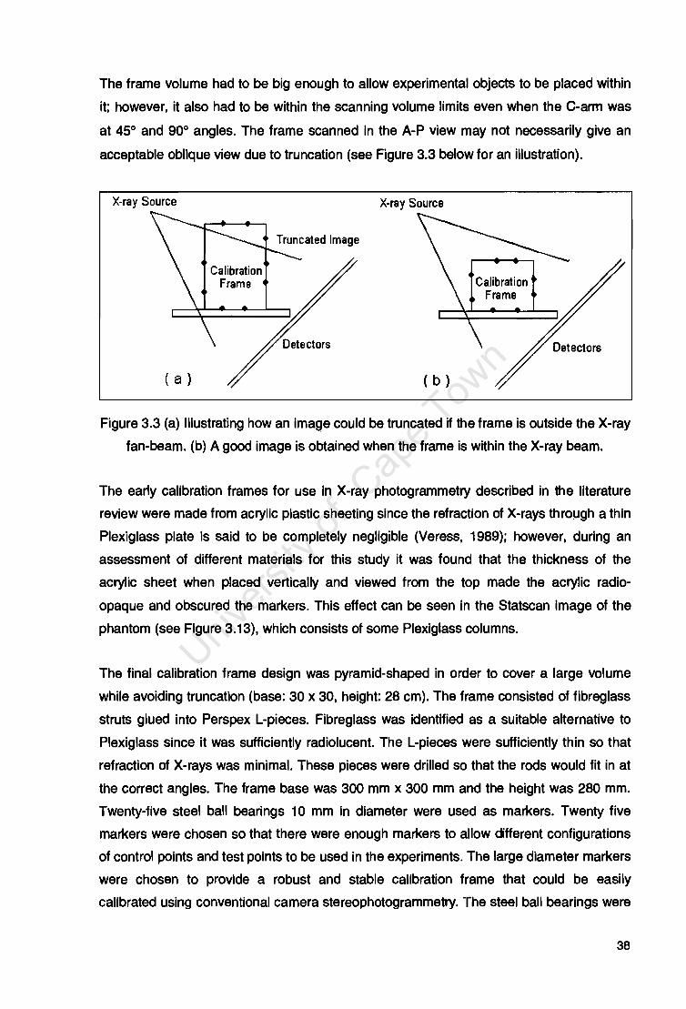
The frame volume had to be big enough to allow experimental objects to be placed within
it; however. it also had to be within the scanning volume limits even when the C-arm was
at 45° and 90° angles. The frame scanned in the A-P view may not necessarily give an
acceptable oblique view due to truncation (see Figure 3.3 below for an illustration).
X-ray Source
( a )
X-ray Source
( b )
Calibration Frame
Figure 3.3 (a) Illustrating how an image could be truncated if the frame is outside the X-ray
fan-beam. (b) A good image is obtained when the frame is within the X-ray beam.
The early calibration frames for use in X-ray photogrammetry described in the literature
review were made from acrylic plastic sheeting since the refraction of X-rays thro~gh a thin
Plexiglass plate is said to be completely negligible (Veress. 1989); however. during an
assessment of different materials for this study it was found that the thickness of the
acrylic sheet when placed vertically and viewed from the top made the acrylic radio
opaque and obscured the markers. This effect can be seen in the Statscan image of the
phantom (see Figure 3.13). which consists of some Plexiglass columns.
The final calibration frame design was pyramid-shaped in order to cover a large volume
while avoiding truncation (base: 30 x 30. height: 28 cm). The frame consisted of fibreglass
struts glued into Perspex L-pieces. Fibreglass was identified as a suitable alternative to
Plexiglass since it was sufficiently radiolucent. The L-pieces were sufficiently thin so that
refraction of X-rays was minimal. These pieces were drilled so that the rods would fit in at
the correct angles. The frame base was 300 mm x 300 mm and the height was 280 mm.
Twenty-five steel ball bearings 10 mm in diameter were used as markers. Twenty five
markers were chosen so that there were enough markers to allow different configurations
of control pOints and test points to be used in the experiments. The large diameter markers
were chosen to provide a robust and stable calibration frame that could be easily
calibrated using conventional camera stereophotogrammetry. The steel ball bearings were
38
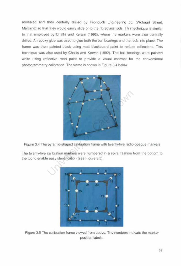
annoaled and then centrally dnlled by Pr<rloudl Engineollllg cc. (Wotrilad Stree1.
Maitland) so thaI they woukl easily slide onlO Ihe hbreglass rods This technique IS similar
to that employed by Challis and Kerwln (1992). where the milikors wore alSo cenlrally
dnlled. An epoxy gluo was used 10 glue boIh Ihe ball bearings and the rods II1tO place. The
trarne was then paillted black using mati blaci<board paint 10 reduce reflectIOns. T<"lIs
tecllruque was also used by Challis and Kerwin (1992). The ball bearings were painled
while USing reflective road paint 10 provide a VIsual contrast for the convonl ior'lal
photogrammetcy calibration. The frame IS shown In Figure 3.4 below.
- • • • • •
• • • • •
• • • < • • •
• • • • • • • •
• Figure 34 The pyramld·SOaped cahbra1ion frame With !Wenly·llve radIO-opaque markers
The twenly·five cahbfluion markers were numbered In a spual faSOlOn from Ihe boilom 10
the top 10 enable easy ldenllticalPOn (see FI!jure 3.5).
Figure 3.5 The calibra tion 'rame viewed trom above. The numbers Indtcale the marker
POSition labels.
"
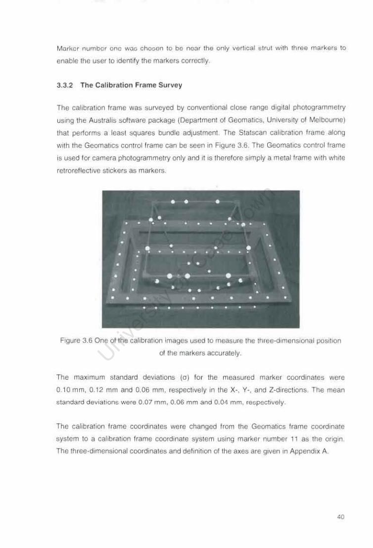
Mmkcr numb"r 0"" w.:m "ho:>on to be Il()ar the only vert ical strut wIth throe markers to
enable lhe user to identify the marllers cor rectly
3.3.2 The Calibration Frame Survey
The cal ibrat ion frame was surveyed by conventional close range dlg,tal photogrammelly
uSing the Austral is soItware package (Department of Geomatlcs, Univers ity 01 Melbourne)
Ihat performs a least squares bundle adjustment The Stalscan cahbrahO" frame along
With the Geomallc5 controll rame can be seen in Figure 3.B. The Geomatlcs cOnlrol trame
is used for camera photogrammelry only and It IS Iherefore simply a metallrame wllh while
retrore!leC1lve stickers as markers.
0 0 0
0 0 0 • • • • • • • '0 •
• • • • • • •
• • • •
• • • • • • • • • • • 0 • • • • • • • • • •
• • • • • • • • • • • • • • • • • •
Figure 3.6 One ollhe cat lbratlon Images used 10 measure Ihe three-dImensional pos.hOn
01 the markers accuralely.
The maXimum standard devlalloflS (0) for the measured marlier coord inates were
o t Omm, 0.12 mm Elnc! 0.06 mm, respectively In the x· . yo. and Z-directions The mean
standard deViations were 0.07 mm. 0.06 mm and 0.04 mm. ,e~p"Cllvely .
The calibrarlOO frame coordinates were changed trom the Geomatics Irame coord inate
syS!em to a calIbration Irame coordmate system using marker number I t as Ihe origin
The Three-dimensional coordinates and deitntllon oIlhe axes are given In AppendiX A.
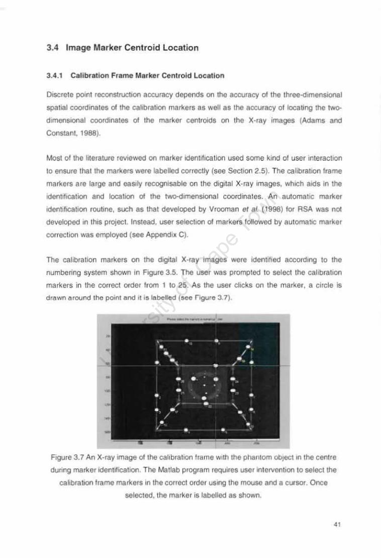
3.4 Image Marker Centroid location
3.4.1 Calibration Frame Marker Centroid location
Otscrete point reconstruction accuracy dependS on the aCC\Jlacy 01 the Ihree-dlmensional
spatial c(l()fClenates 01 the calibrallon markers as well as the accuracy of locating the tW<r
drmensional coordinates of the marker cenlrolos on the X'ray Images (Aclams and
Constant. 1988).
Most of the literature ICVlewecl on marker Identrficatlon used some kind 01 user IIllelaction
to ensure thallhe' markels were labelled cOfrectly (see Section 2.5). The calibrallon frame
markers are large and eaSily recognisable on the digital X·ray images, whICh aids In lhe
iden"licalion and Iocabon 01 lhe two-dImensional coordinates. An automatic: markel
idenhhcalion roullne. su:::h as lhat developed by Vrooman er a/. (1998) fOf RSA was nol
deveKlped In thIS project Instead, user se~tlon 01 markers followed by automatIC marker
coooction was employed (see Appendix C).
The calibration markers on the tIigotal X·ray images were identified accord'ng to the
numbering system shown in Figure 3.5. The user was prompted to select the calibration
markers in Ihe correct Ofder from' \025. As the user clicks on the marker, a circle is
dr ... wn ... round lhll pornt and II ,5 labeled (aee ng • .rrll 3.7).
FlQUre 3.7 An X·ray image of the calibration frame With the phantom object III the centre
dunng marker idenlrfic:atlon. The IIoIatiab program requires user intel'llenllon \0 select the
ca6brallOn lrame markers In the correc1 order USing the mouse and a ClnOf. Once
selected. the marker Is labelled as shown.
"
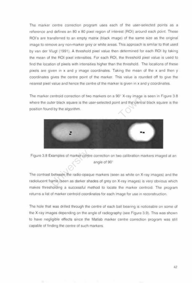
The marker cenlre corrll(1lQn program uses each of Ihe user-seleCled points as a
reference and defmes an 80 x 80 pixel regIOn of mimes! (ROI) around each poln!. These
ROl's are Iransferred to an empty matnx (black Image) of the same SIZI! as the onglnal
Image 10 remove any non-marker grey or white amas. This approach ~ Slmllar to that used
by van dec V1ugt (lggl)_ A threshold pl xe! value Ihen determined lor each ROI by taking
lhe mean 01 the AOI PiXel mtenslties for each AOI. the threshold pl~el value is used to
find the locatIOn of prxels llilth ontenSllleS hlgiler than the threshold The locations of lhese
pixels are gwen m x and y ,mage coordmates. Taking the mean of the x and then y
coordinates gives the centre peonl of tile marker Thrs value IS rounded off to 9'1/(1 the
nearesl prxel value and hence the centre of the marker is grven In x and y coordinates
The marker centrOId correctIOn of two markers on a 90 X-ray Image IS seen In figure 3.8
where the outer black square rs the user-selected pornl and the central black square ~ the
posrtlon found by the algor1thrn
Figure 3.8 Examples of marker centre COfrectron on two cahbrahon markers Imaged al an
angle of 90
The contrast between the rado-opaque markers (seen as whole on X-ray rmages) and the
radfolucent flame (selin as darl<:er stlacles of grey on X-ray Images) Is very obVrous wl-llch
makes th,csholdll'9 a successful mtlthed to locate the marko, centroid The pr'ogram
w tums a Irst of marl<:er cenlrord coorclrnatcs lor each rmage lOf use In .cconslrUCf.o<l
The hola thai was dnlled through the centre of each ball bearing IS notICeable on some of
the X-ray Images dcpllnding on the angie 01 racflOgraphy (see Figure 3_9)_ This was shown
to have negligib le effects since the Matlab marker centre Co«ectlOn program was stili
capab le of "ndlng the centre of such markers
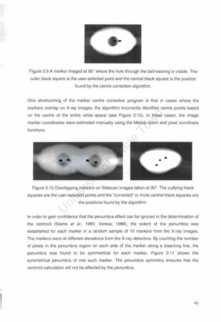
Figure 3.9 A mar1<er Imaged at 90° wheu:! the hote through the ball-beaflng is visible. The
outer black square IS tho user-selected point and the central black square is Ihe poSition
found by the centre correction algorithm.
One shortcoming 01 the mar1<er centre correction program is that in eases where the
mar1<ers ovel1ap OIl X-rav images, the algorithm Incorreclly identijies centre points based
on the centre of the entire white space (see Frgufe 3.10). In these eases, the Image
marker coordina tes Wtire estimated manually using the Matlab ~oom and pixel coordinate
Itrnctloos.
Frgure 3.10 Ovel1apprng markers OIl StalScafl rmages takefl 0190". The outlying black
squall:~S are the user-selected porfllS and the '"corrected'" or more central black SQuares are
the positions loufld by the algontlun.
In order to gain COfltideoce that the pefll.lmbra eltect can be lQrtored in the determrnatlOfl of
the centrOId (Slama el 81., 1980; Veress, 1989), the e~tem 01 the penumbra was
established for each marker In a random sample 01 10 ma/kOis from the X-ray Images.
The marllers were at different elevabOOB from the X.ray Oeteclors By coufl!ing the flI.Imber
OJ pixels in the peflumbra reg;oo on each side 01 the marlier along a bisecting line. the
penumbra was lound to be symmetrical lor each marlier. Frgure 3.11 shows the
symmetrical penumbra 01 one SlICh marker The penumbra symmetry ensures that the
centrOid calculation will not be affected by the pefll.lmbra.
"
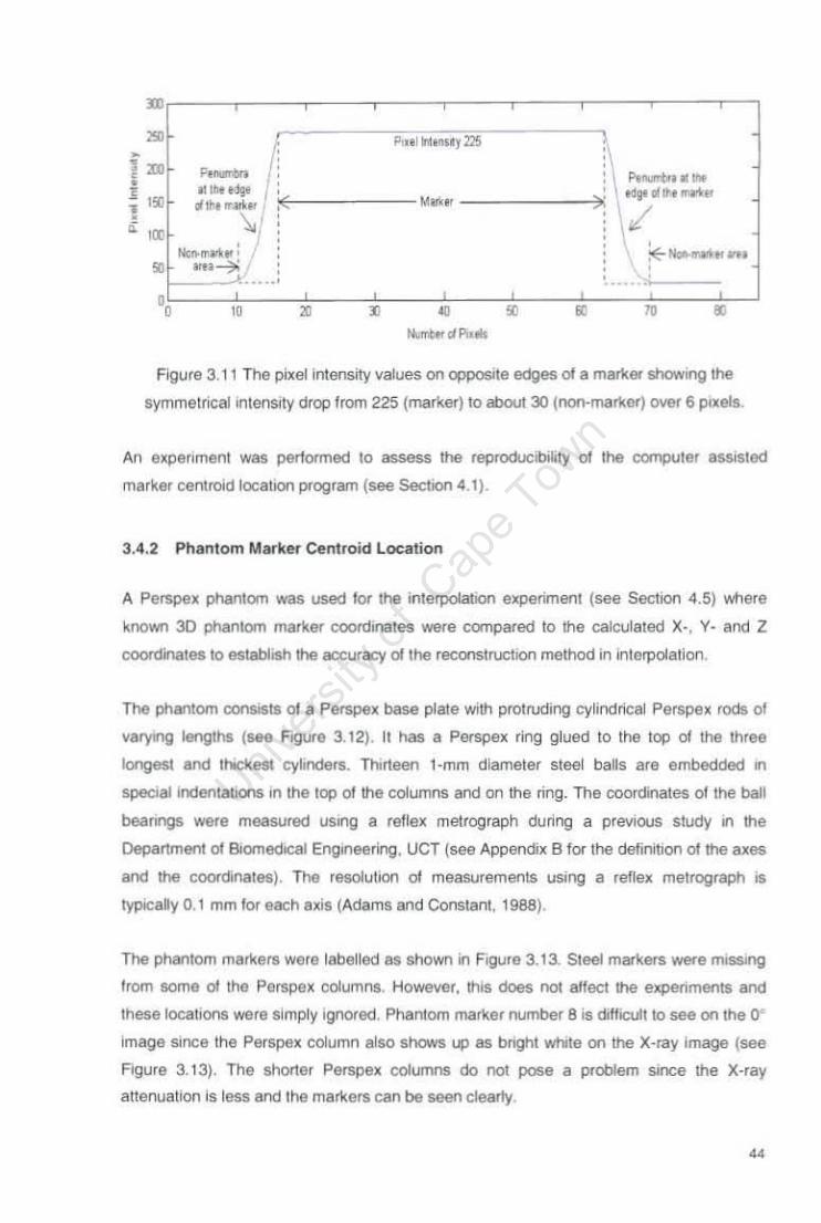
" '" •
• Ii I" ,- , • , • <
MtI,,,,I9o I , • ,. ...'h. r ...... . <
,re \ , • Ncn-mOl\ .. ' • ..... --:'»i , , ..... ,
00 m • • Figure 3.11 The pixel intensity values on opposite edges of a mar\(er 6howlng the
symmetrical ~lens.ty drop from 225 (marker) 10 about JO (noo·malker) ovo( 6 PIXelS.
An experiment was per10rmed 10 assess !he reproducibility 01 the computer assisted
marker CenlrtHd locatlOl'l program (see Section 4.1).
3.4.2 Phantom Marker Centroid Location
A Pel'Spex phantom was used lor the interpolation experiment (see SectiOn 4.5) where
known 30 phantom marlr.er coordinates wm8 compared to the calculated X- . y. end Z
coordinates to establish the accuracy 0/ the lecQOStructlOll method in interpolation.
The phantom OOOSISts 01 a Perspex base plate with protruding cylindrical Perspex rods 01
V8r'y1Og lengths (see FtgUfe 3.12). It has a Perspex ring glued to the top of the three
\ong8$l and thockest cybnders. Thneen I-mm diameter 51001 bans are embedded in
speciallndentatJOl1S in the top 01 the ~umns and on the ring. The coordinates of the ball
bearr.gs were measured usoog a reUex me\rograph during a previous study Ofl the
Department 01 BiomedlClll Engmeering. UCT (see Appendix B for the definition of the lIXe5
and the coordinates). The resolution 01 measurements using a rellex metrograptl is
typtCsRy 0.1 mm for each axi$ (Adams and Constant, 1988)_
The phantom markars wele labetled as shown in Figure 3.13. Steel markers W6fe mrs&ng
Irom some of the Perspex Columns. However, !his tioes not atfecl the elq>efiments and
these locations were simply ignored. Phantom marker number 6 IS difficult to see on the 0-
image since the Perspex column also shows up as bright white 00 the X-ray image (see
Figure 3_ t3). The shorter Perspex columns do not pose a problem Since the X-ray
attenuallon Is less aod the marker!! can be seen clearly
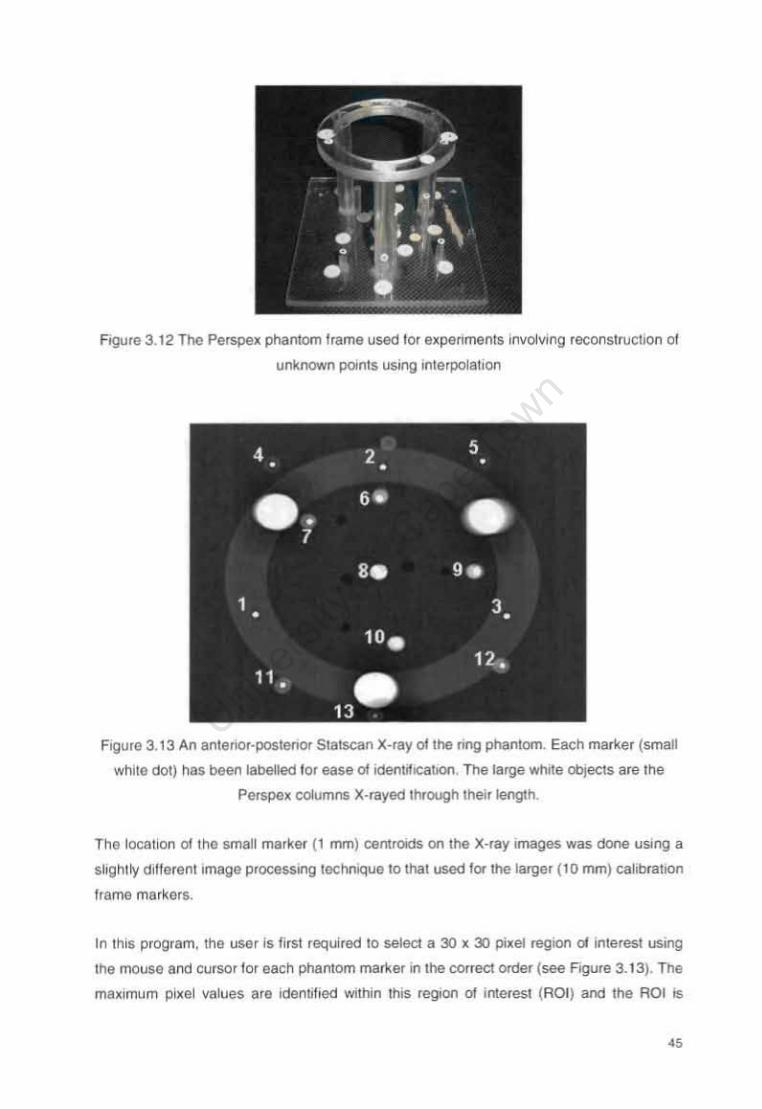
-s;s-.. .. ~.--• ';"l' :r,· . ... . .! Q
• • " r •
e -'0--
Figure 3.12 The Per&pex phantom Irame llSOO lot oJpenmenls jrwojyjng r8COflstruclron or
unknown poinls using inlerpojetlOll
4 2 5 • • •
•• 6" • 7
Se 9 .. , 3 • •
'0. 12-.
". '3·
Figure 3.13 An anterior-postenor Statscan X·fay ollhe nng phantom. Each marker (small
while dot) has been labelled l or ease of Ident~lCallOn. The large while objects are the
Perspex columns X-rayed through Ihelrleoglh
The localion of the small marker (1 mm) cemrOlds on the X-ray .mages was done using a
slightly dlUerenlrmage proceSSJf19 tocMIQUe 10 thaI used lor the larger (10 rnm) calIbratiOn
frame markers.
In this program. the Usef is firs! required 10 select a 30 x 30 pixel region of interest uSing
the mouse and cursor lor each phantom marker 111 the coned order (see Figure 3.13). The
maximum pixel values are Idenhhed wUhm Ihis reg.on 01 imeresl (ROI) and Ihe ROt is

converted Iota a binary Image whele the maXIITJ.lm pxel values with a connectIVIty 01 4
Pixels are given a value t (while) and the other pKeis are changed to 0 (black). The Inbt.ult
Matlab lunctlon "lmleature" IS then used to fond the centre of mass 01 each while marl<er
reglOll. Based en the VlSualmspectlOll of 9t selected markers (13 markers in each of the 7
radiographs), the program accurately round the marker cen1res as long as there _8 rro
other Interlerences such as overlapping markers. m~lIkelS Wllhm the 30 x 30 Pixel feglOll
of Inleres1 or Interlerences lfOm the radro-opaque Perspex columns ($8tI Figure 3. t4).
Frgure 3. t 4 The marker cenlre correction 01 a t mm steet marker emb8(kled In a Perspex
rod The ooter black square is the user selected point and the central square IS the
corrected cenlre
3.5 Reconstruction Software
Computer programs wntten in Matlab were used to perform the three dlmenSlonat
recOrlstruction as described by van Geems It997) (see Append iX C). The krrown three·
dimensronal coordinates ot the COrltrot points were USed as InputS as well as the
corresponding two dimenSional coord'nates 01 the same pOints and the lwo-d,mellSlonal
coordinates of the leSI POints The program uses junct ions to generate the reqUired matrix
9JVBr1 by the algoflthm In SeCiIOfl 3.2.1
The OUtput 01 the program IS a matrix conta ining the ca lcula ted marker coordinates The
program compares these calculated coord inates to the known coord inates and provides
the X. Y and Z errors for each poiI1t.
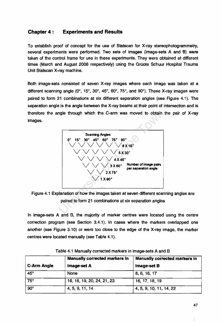
Chapter 4: Experiments and Results
To establish proof of concept for the use of Statscan for X-ray stereophotogrammetry, several experiments were performed. Two sets of images (image-sets A and B) were taken of the control frame for use in these experiments. They were obtained at different times (March and August 2006 respectively) using the Groote Schuur Hospital Trauma Unit Statscan X-ray machine.
Both image-sets consisted of seven X-ray images where each image was taken at a
different scanning angle (0°, 15°, 30°, 45°, 60°, 75°, and 90°). These X-ray images were
paired to form 21 combinations at six different separation angles (see Figure 4.1). The
separation angle is the angle between the X-ray beams at their point of intersection and Is
therefore the angle through which the C-arm was moved to obtain the pair of X-ray
images.
Scanning Angles
0° 15° 30° 45° 60° 75° 90° V V V V V V6X15°
V V V V V5X300
V V V V 4X45° V V V 3 X 60° Number of image pairs
per separation angle V V 2X75° Vi X900
Figure 4.1 Explanation of how the images taken at seven different scanning angles are
paired to form 21 combinations at six separation angles
In image-sets A and B, the majority of marker centres were located using the centre
correction program (see Section 3.4.1). In cases where the markers overlapped one
another (see Figure 3.10) or were too close to the edge of the X-ray image, the marker
centres were located manually (see Table 4.1).
Table 4.1 Manually corrected markers in image-sets A and B
Manually corrected markers in Manually corrected markers in
C-Arm Angle Image-setA Image-setB
45° None 8,6,16,17
75° 16,18,19,20,24,21,23 16, 17, 18, 19
90° 4,5,9,11,14 4,5,9,10,11,14,22
47
In image-set B. with the C-arm at 60° and 75°. markers 23 and 24 were truncated and so
were not present on the X-ray images. With the C-arm angle at 90° (scanning laterally).
markers 20 and 21 were truncated (see marker labelling in Figure 3.5). This problem was
not experienced when image-set A was obtained. and so this truncation is possibly due to
slight changes in the operating table set-up between scanning image-sets A and B. These
four markers have been excluded from all the experiments.
The method of establishing the accuracy of point reconstruction varies among researchers
depending on the information available (Challis and Kerwin. 1992). Some researchers
compared calculated distances with measured distances (Adams and Constant. 1988).
while others compared calculated point coordinates with measured coordinates (Wood
and Marshal. 1986; Plamondon and Gagnon. 1991; Challis and Kerwin, 1992). The
comparison of distances is mainly used when the object coordinate systems and
calibration frame coordinate systems differ. In the Statscan experiments. marker
coordinates were compared to measured coordinates except in phantom point
reconstruction (see Section 4.5). where the marker distances from an origin marker to
other markers were compared with measured distances.
The following experiments were performed to assess the suitability of Statscan for X-ray
stereophotogrammerty:
1) The reproducibility of locating two-dimensional marker centroids using two images
taken at 0° and 90° from image-set B.
2) The reconstruction of control points (points on the calibration frame that were used
in determining the transformation parameters) using image-sets A and B.
3) The reconstruction of test points (non-control pOints on the calibration frame) using
image-set B only.
4) The reconstruction of test points (non-control points on the calibration frame) using
extrapolation and image-set B only.
5) The reconstruction of phantom test points that lie within the control point volume
using interpolation and image-set B only.
48

4.1 Reproducibility of the 2D marker centroid location
The reproducibility of the manual marker selection and the marker centroid correction
program was tested by assessing the marker selection results of three independent
operators. Each operator selected the 15 markers on the image-set B, 0° and 90° images
three times according to the numbering given in Figure 3.5, with the exception of markers
numbered 4, 5, 9, 10, 11, 14, 20 and 21. These markers were excluded because they
overlapped on the 90° image and gave obviously incorrect results when using the marker
centroid correction program. The results are given as the mean standard deviations of the
x and y image coordinates for the sets of manually selected and corrected markers.
To establish the effect of the marker centroid identification on the three dimensional
reconstruction, the nine sets of two dimensional marker coordinates obtained from manual
marker selection and the centroid correction program as described above were used to
reconstruct the 15 control points. The results are given as the mean standard deviations of
the nine sets of X-, Y- and Z-coordinates for each identification technique.
4.1.1 Results: Reproducibility of 20 marker centroid selection and correction
The mean standard deviations for the manual selection of the 15 markers (nine sets per
image) were 0.46 and 0.45 pixels (0° image), 0.31 and 0.25 pixels (90° image) and 0.39
and 0.35 pixels (0° and 90°) for x and y respectively. The image resolution is
approximately 0.2 mm per pixel, so the mean standard deviations for x and y image
coordinates when manually selected can be given as 0.08 mm and 0.07 mm respectively
(see Table 4.2).
The mean standard deviations of the x and y image coordinates for the nine corrected
marker selections were 0.42 and 0.09 pixels (0° image) and 0.53 and 0.09 pixels
(90° image) in the image x and y directions respectively. In the 0° scanning angle, the
image x axis corresponds to the Statscan Y axis and the image y axis corresponds to the
Statscan Z axis (direction of travel). The total mean standard deviations for 00 and
90° images are 0.47 and 0.09 pixels (approximately 0.09 mm and 0.02 mm) in the x and y
directions respectively (see Table 4.2). It was noted that both the x and y errors were
generally greater for markers that were further from the X-ray detectors, than for those
closer to the detectors (see Table 0.1, Appendix 0).
49

II . \
Table 4.2 The mean standard deviations for the 20 coordinates of the markers identified
manually and using the marker correction program
x (pixels) y (pixels) x (mm) y(mm)
Manual marker centroid identification 10.39 0.35 0.08 0.07 Marker
10.47 program identification 0.09 0.09 0.02
The mean standard deviations for the 3D reconstruction of the nine sets of 15 markers
were 0.05 mm, 0.07 mm, 0.05 mm for X, Y and Z-coordinates respectively when using the
manually selected 20 coordinates, and 0.07 mm, 0.06 mm and 0.02 mm for X, Y and Z
coordinates respectively when using the corrected marker coordinates (see Table 4.3).
Table 4.3 The mean standard deviations for the reconstruction of 3D coordinates of the
markers identified manually and using the marker correction program
Manual marker centroid identification Marker centroid correction
ro ram identification
X (mm) Z (mm)
0.05 0.07 0.05
0.07 0.06 0.02
The X direction manual marker centroid identification gives a lower standard deviation
than the marker centroids correction program. The marker centroids correction program
should be optimised to at least be an improvement on the manual method.
4.2 Reconstruction of control points
The reconstruction of points that are used in the calculation of the transformation
parameters (control points) does not fully test the reconstruction accuracy of this method,
although it does provide information about the accuracy of the mathematical technique
and any unaccounted for aspects of the reconstruction, e.g. noise (Challis and Kerwin,
1992). The reconstruction of control points has previously been used as a measure of
accuracy by Wood and Marshal (1986) and Hatze (1988). In this experiment, the
reconstruction of two independent image-sets (image-sets A and B) was used to assess
the repeatability of the method.
The three dimensional reconstruction results are used to test repeatability instead of
merely comparing the marker centroids from the X-ray stereo-pairs (Wang et al., 1996)
50
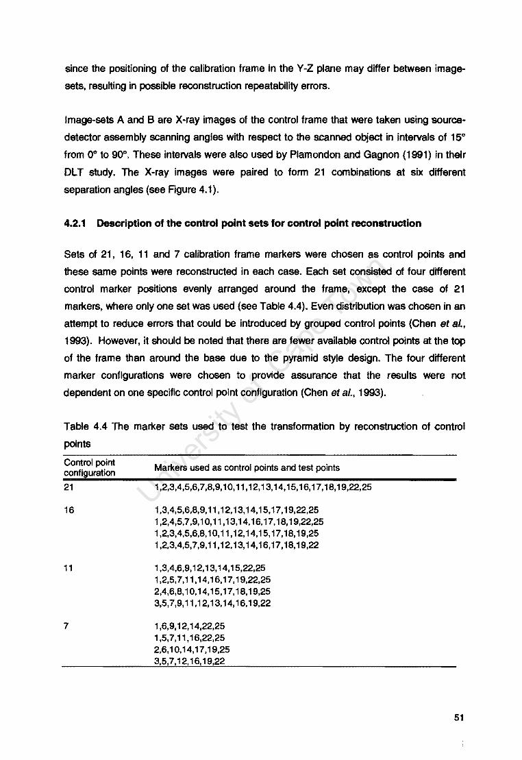
since the positioning of the calibration frame in the Y -Z plane may differ between image
sets, resulting in possible reconstruction repeatability errors.
Image-sets A and 8 are X-ray images of the control frame that were taken using source
detector assembly scanning angles with respect to the scanned object in intervals of 15°
from 0° to 90°. These intervals were also used by Plamondon and Gagnon (1991) in their
DLT study. The X-ray images were paired to form 21 combinations at six different
separation angles (see Figure 4.1).
4.2.1 Description of the control point sets for control point reconstruction
Sets of 21, 16, 11 and 7 calibration frame markers were chosen as control points and
these same points were reconstructed in each case. Each set consisted of four different
control marker positions evenly arranged around the frame, except the case of 21
markers, where only one set was used (see Table 4.4). Even distribution was chosen in an
attempt to reduce errors that could be introduced by grouped control points (Chen at aL,
1993). However, it should be noted that there are fewer available control points at the top
of the frame than around the base due to the pyramid style design. The four different
marker configurations were chosen to provide assurance that the results were not
dependent on one specific control point configuration (Chen at al., 1993).
Table 4.4 The marker sets used to test the transformation by reconstruction of (:ontrol
points
Control point configuration
21
16
11
7
Markers used as control points and test points
1,2,3,4,5,6,7,8,9,10,11,12,13,14,15,16,17,18,19,22,25
1,3,4,5,6,8,9,11,12,13,14,15,17,19,22,25 1,2,4,5,7,9,10,11,13,14,16,17,18,19,22,25 1,2,3,4,5,6,8,10,11,12,14,15,17,18,19,25 1,2,3,4,5,7,9,11,12,13,14,16,17,18,19,22
1,3,4,6,9,12,13,14,15,22,25 1,2,5,7,11,14,16,17,19,22,25 2,4,6,8,10,14,15,17,18,19,25 3,5,7,9,11,12,13,14,16,19,22
1,6,9,12,14,22,25 1,5,7,11,16,22,25 2,6,10,14,17,19,25 3,5,7,12,16,19,22
51

4.2.2 Results of control point reconstruction
The transformation error is expressed as the mean absolute difference between the known
three-dimensional coordinates, as measured by the Australis system {see Section 3.3.2),
and the calculated coordinates of each marker. The mean absolute errors (ex ,ey,ez) were
calculated as shown below for each stereo-pair to allow analysis of the effect of the
separation angle.
where:
n
Xci 'YCi ,Zci
(9)
(10)
(11 )
number of points for each series (i.e. 21, 16 x 4, 11 x 4,7 x 4)
3D coordinates of the points measured by the Australis system
3D coordinates calculated using the transformation parameters
The program uses linear fitting on the two stereo X-ray images to obtain two reconstructed
Z-coordinates for each marker since the object Z-coordinate has a linear relationship with
the image y coordinate. The Z-coordinate (Zci) is taken as the mean of the two
reconstructed Z-coordinates for each marker. The resultant error (eRes ) was calculated as
shown in equations 12 and 13.
(12)
where: (13)
In addition to the mean absolute errors, the maximum absolute errors were also calculated
for the X, Y and Z coordinates and are given in Table D.2 and D.3 in Appendix D.
52
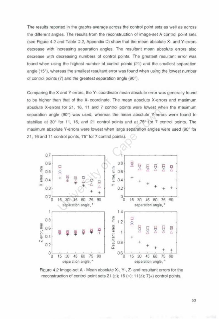
The results reported in the graphs average across the conlrol point sets as well as acr05S
!he dillerent ar'lgles. The results from the reconstrucTion 04 Image·set A control point sets
(see Figure 4.2 and Table 0 .2, Appendix OJ show that the mean absolute X· and Y·errors
decrease With IncreaSing separa tion angles. The resultant mean absolute errOrs also
decrease with decreasing numbers 01 conTr~ poInls. The greeTest resultant error was
found when uSIOQ The htghesl number 01 control poinTs (2 T) and the smallest separation
angle ( T5~). whereaslhe smalleST resultant error was found when using the towest number
01 control poI/lts (7) and the greatest separation ar'lgle (90°).
~nr'lg the X and Y errors, the Y- coordrnate mean absoluTe efror was generally found
to be higher than that 01 the X· coordinate. The mean abs~ule X-errors and maximum
absolute X·errors for 21. 16, T 1 and 7 control poInlS were lowest when the maximum
separation angle (90") was used, wtrereas the mean absolute Y-errors were found to
slabillSe at JO' for 11 . 16. and 21 conlrol pornts and at 75' for 7 control points. The
maXimum absolute Y-errors were lowest when large separation angles were used (90° for
21 , T6 and 11 control porniS. 75· 'or 7 control points).
07
" 08 ~ ~ 2 ~ ~ , 0 e £ 05 e e " ! " + ~ • C , "
+ • ~ C 0 • + • • + " > +
03 0.2 + + + + +
"0 "., "Ol " OJ 00
" ., " Ol " OJ sepiritlOn .~. ' sepa.;llIon angle .•
I " 08 e 0 e " e , " ~ 0 ! § ~ 2 § " ! ~ ~ ~ ~ + • ~
" " + • • ~ N , 0.8 +
" • • + a + + + 00 "., "Ol "., "0 " ., " Ol "
., sepilillon atlQtl , • l eparilron angle , ·
Figure 4.2Image-sel A - Mean absolute X-. Yo, Z- and resultant errors lor the reconstruction 01 COOIrol point sets 21 (): 16 (0 ); 11 ( .... ); 7(+) control pornts.
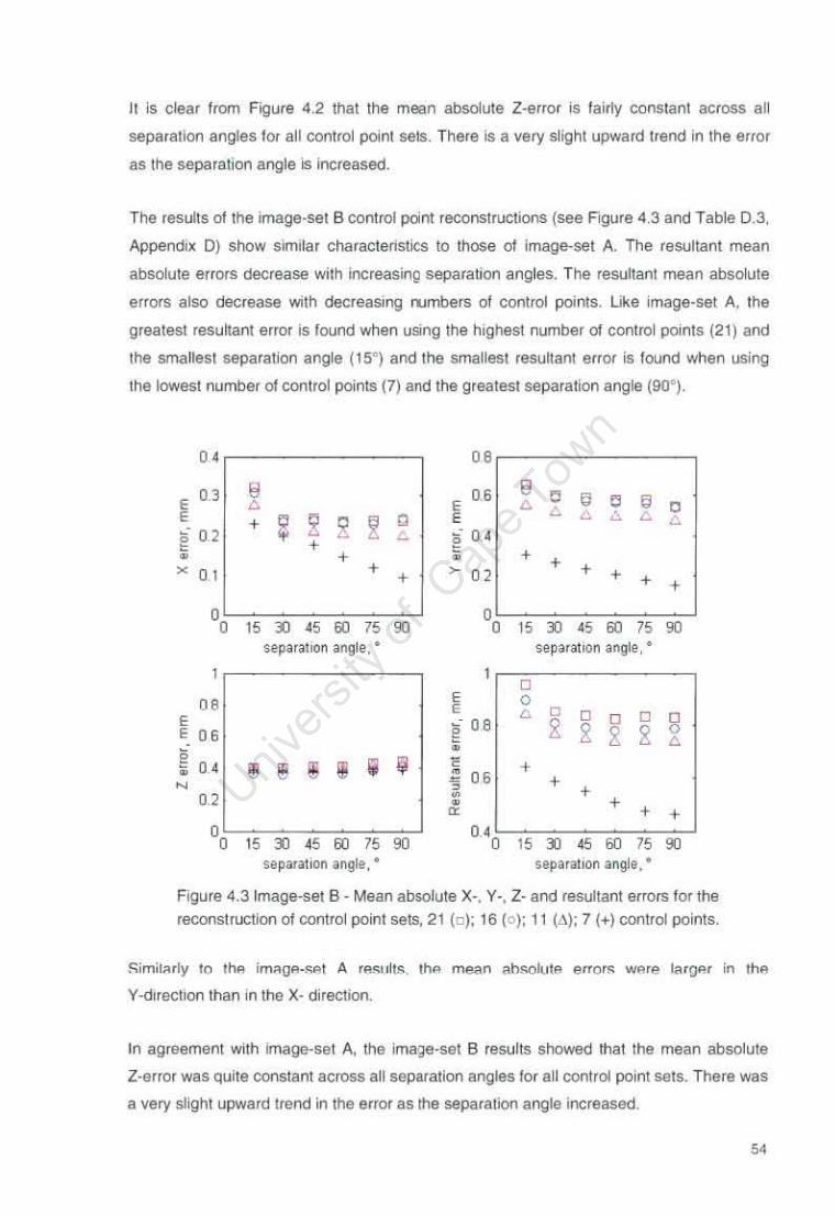
H Is clear from FlQure 4.2 that the mean absolute Z-error is fairly constant across all
sepa!ation angles tor all control point sets. There Is a very slight upward tlend in 1he error
as 1he separation angle is Increased.
The results of the image·set 6 control pcint recons1ructions (see Figure 4.3 and Table 0 .3.
Appendix 0) show similar characlenstics to those of Image-set A. The reSIJltant mean
absolute errors decrease wilh increasing separation angles. The resultan1 mean absolute
errors also decrease with decreasmg rumbers of control points. Like image-set A. the
greatest resunant error is found when using the highest number 01 control points (21) and
1he smalles1 separation angle (15°) and the smallest resultant error is found when using
the lowest number 01 control points (7) and the greatest separation angle (90").
" DB
0.3 8 0.6 8 0 " 0 " E 0 , 6 0 , ? ~ ~ 0 , 6 " 6 6 + R " , 02 " <5 o.
" + " • + • + + • " + > 02 + + + + +
00 15 ., " OJ 75 OJ 00 15 .,
" OJ 75 OJ sepa r~HM angle. ' separation angl2. •
1 0
DO ! 0 , 6 0 0
R 0 8 ~- 08 & g g , 06 ,
6 g •
" ~ ~ II II ij ~ • + • • 06 • + N , + 02 • • + • + + 00 15 .,
" OJ 75 OJ 0.4
0 15 " " OJ 75 OJ separatIOn angle .• separation angle.'
Figure 4.3Image·set B · Mean absolute X-. Yo. Z- and resultant errors for the
r&construction of control poil'lt sets. 21 (0); t6 (0); It (~); 7 (+) COfltrol poinls.
!';imil"rly 10 Ih" im"g"_"'" A 'a«lIlt8 th .. me3n aho;olutFl erro", WFlre ta r(}FIr in the
Y-dlrection than In the X· direction.
In agl8ement with image-set A, the Ima·:1Q·set 6 results shewed that the mean absolute
Z-e f/or was qUlle constanl across all separation an91eslor all cont rol point sets. There was
a very slight upward trend in the enor as the separation angle Increased.
AUhougtJ !he e<rOf !rends lor Image-sets A and B wele conSistent_ the error magnitvdes
differed between the IWO Image-sets. In all cases. Iowel mean absolute errors wllre
rOCOfded for Image-set B Ihan Image-set A. The mean differences between the mean
absolute X-, Y- aod Z efrors 01 image-set A and B WIIre O. t e mm, 0.14 mm and 0.12 mm
.t;spectNely Imagtt-sel B was oblalned a lew months afte. Image-set A and the
dil1erences in errOl" could be annbuted to improvements on the Statscan Image
leconstruclion software. The differences in mean absolute enor and maximum abSOlute
81rOl between Image-sets A and Bare labulaled in Table 0.4 in AppendiX 0 101
compleleness. Image-set B was chosen 10 be used for the rest of the expenments Sloce it
yie lded better ovelall accuracy than Image·set A
To summarise. in this expenment we have seen that when points Ihat WIlle used In the
derivatfon 01 transformation parameters (control points) were reconstructed. the lowest
mean absolute errors were observad when uSing the lowest numbel 01 control points and
the largest separation angle, The low e rror when uSing large separation al'lQles IS In
agreemenl With the literature and the low error when lew control points are used can :Ml
eJlPlaoned by the "over-fltllng" 01 the DL T equations to the lew control pointS. The observed
accuracy can therefore not be taken as a Irue representatiofl 01 uflknown po'n!
reconstrlJCllOfl
4.3 Reconstruction of test points using calibration frame markers
In Ihls expenment. the reconstr1.IChon of non-conlrol point cahbratlOfl Irame marllers (lest
painlS) was used 10 teslthe accUiacy ollocallng unknown points These 1'lOIl-coniroi poiO/s
were not used In eslabhshong the transformatlOfl parameters. Thls appfoach cJ
leconslructlng non-control poon' cal ibration marl<ers has been LJ$ed by severallesearchers
on lhe pas' to establish the true accuracy of reconsttUC1lng unknown poll1l!> (ChallIS and
Kerwin, 1992; Plamondor1 and Gagnon, 199t; Chen elal. 1 994). Image-SlIt B was used III
thiS experiment
4 .3. 1 Descript ion ollhe con trol pOinl sets lor test poinl reconstruc tion
The same se ts 01 16. t 1 and 7 carlb/allon 1rame marllers as on Section 4.2 were chosen as
control points but II1stead of leconstrucllng lhase same points. ',ve dlfl erent POintS were
reconsuucted (see Table 4.51_
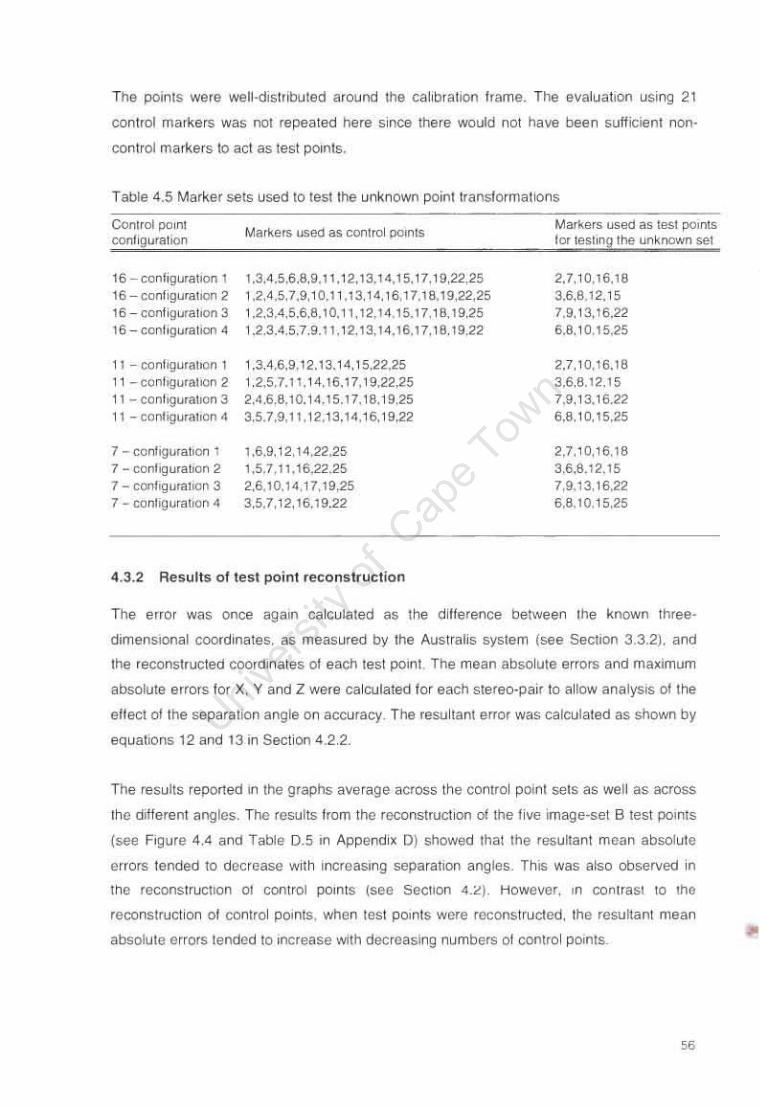
The points were well·dlslutxl!ed around the cal ibration frame. The evaluation using 21
control markers was nOi repeated here since there would not have been su/ticlent non·
conlro! markers to act as test POints.
Table 4.5 Marker sets used to test the unknown point transformat ions
Conlrol po int cont igurahon
16 -con1igurstlon 1 16 -conflgurallon 2 16 - configurshon 3 16 - ccnfiguralioo 4
11 - confIQurahCn 1 I I -conhguraloon 2 11 - conhgura!Ion 3 11 - conhgura!Ion 4
7 - confIQuratlon 1 7 - conhgurahOn 2 7 - coofigufililon 3 7 - conhgura!Ion 4
Markers .... oo as cormol polnlS
t .3.4.5,6.8.9. t 1. I 2.13.14. 1 5. I 7. I 9,22.25 1.2,4.5.7.9, 10.1 I .13, 14.16,17.1 8.19,22,25 1 .2.3.4.5.6,6. 1 O. 1 t, 12.1 4 15.17, I 8, HI.25 1 .2.3.4.5.7.9. 11. I 2. 13. 14. 16. t 7. 18. 19,22
I .3.4.6.9. 12. 13. I 4, 1 5,22.25 1.2.5.7.1 I. I 4.16.17.19.22.25 2.4.6.6.10.14.15. t 7. 16. 19,25 3,5.7.9.1 1.12.13.14.16.19,22
1.6.9, I 2,1 4,22.25 1.5.7.11.16.22.25 2,6.10.14, 17,19,25 3.5.7,12.16.19.22
4.3.2 Results 01 test point reconstruction
Markers USed as test pomts for tesl",\! the un~nown sel
2.7, 10.16.1 6 3.6,6.12. 15 7.9.13,16.22 6.8. 10.15.25
2.1,10,16.16 3.6,8.12.15 7.9.13.16.22 6.6.10.15.25
2.7,10.16.18 3.6.8.12.15 7.9.13,16.22 6.6.10. 15.25
The error was once aga,n ca lculated as the dltterence between Ihe known three·
dimenSional coordinates. as measured by the Australis system (see Section 33.2). and
Ihe reconstructed coordinates ot each test point The mean absolute errors and ma~lmum
absOlute errors lor X. Y and Z were ca lCUlated lor each stereo-pair to allow analYSIS of the
effect of the separallon angle on accuracy. The resu ltant error was calculated as shown by
equations 12 and t3 in Section 4.2.2.
The results reported In the graphs average across the control point selS as well as across
the ditferent angles. The results from the r(!ConstructlOn of the five image-set Blest pomts
(see Figure 4,4 and Table 0.5 In Append i ~ 0) showed that Ihe resultant mean absolute
errors tended to decrease wllh increaSing separation angtes. ThIS was also observed in
Ihe re<:onSlrUCllOn 01 contrOl POints (see Section 4_~ )_ However, on conl raSI to the
reconstruct ion ot control POintS. when !Cst POints were reconstructed, the resultant mean
absolule errors tended to Increase with decreasing numbers at contro l POIntS. •
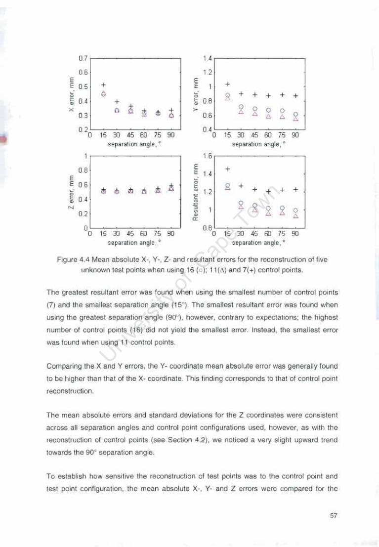
0.7 " 06 12 , ,
+ , 05 + , g • , s + + + + + " + • 06 • • • 0 • • • + > 2 ~ 0 0 0.' 0 06 • 0 R "0 15 " " 60 75 ., "0 15 " " 60 75 .,
separ(l1lon angle,' separal.on angle, '
1 " 06
, + ,
" , , , 06 • 0 +
~ • • • • • 12 + + + +
" • • ~ • 2 2 N , 2 0
" • • 0
" 00 15 " "'" 75 ., 06
0 15 .., " '" 75 '" separation angle , ' s~pimdlon .. ngle,·
Figure 4.4 Mean absolute X-, Y-, Z- and .&sultanl CHorS for the reconsl(lJcflon 01 live unknown lest points when uSing 16 ( ): 11(,,) and 7{ t ) control poilns.
The greatest resultant error was found when usmg Ihe smallesl number 01 control points
{7} and Ihe smallest separation angle (15"). The smallest resultant error was found when
using the grealesl separation angle (90"), however. contrary to expe<:talions; the highest
number 01 control points (16) did not ylekl the smallest error. Instead, Ihe smallest error
was found when using 11 conlrol points.
Comparing Ihe X and Y errors, the y . coordlnale mean absolute error was generally found
\0 be higher than that 01 the X- coordil'\ate. This finding corresponds to that 01 COfltrol point
reconstrUclion.
The mean absolute errors and standard deviations lor the Z coordinates were consistent
across all separation angles and control point configurations used. however. as with Ihe
r&coostruclion of COfltroi points (see Section 4.2). we noticed II very slight upward trood
towards the go' separation af1gte.
To establish how sensrHva the reconstruction of last points was to the control point and
test point configuration. the mean absolute X-. Y- and Z errors were compared tor Ihe

reconstruction of test pdnts using 16 control points in Ihe foor different conhgural101'\s
(defined In Table 4.5). The configurations are different well·distnbuted arrangements 01
control and test points aroond the frame.
It is clear from Figure 4.5 that the configuration 01 control points and test points influenced
the reconstruction of test points.
"' • " "' ! ". ~ ! , ,
! '" • 0', . ~ .~ .
i ~ 09 ~ .... - 0 0 " • "' " ....
~ .... . • '. ""-+. , 0 NOs!; + ..... • • • "" -.. ... .. ~ . "" ' 0 • • . +.. . "
10, R .1) ' ,+-.~. ,. '" " ~ ,
1 0
" "' 0" ..,. ..... i" 0 0 0 • , 0
0 o .. "6 0 • 0 , , b 0 •
, P" :i 05 • f " 0 0 G 0
"' , " ~ " ~ " " • ,
" ~ • ~ " .. '~, " ~ " .. " .. S.~"MrctI"'" • Sop ............ . s., ....... 0IIfIt •
'" I" I"
Figure 4.5 The mean absolute (a) X'. (b) y. and (c) Z errors fOf the reconstruction of 5 test
pornts USing 16 control po.-rts In dilferent configurations; configuraliOfll (r ),
configurallOn 2 {r Io configuration 3 (.1). configuration 4 ( .. )
(ConflgIJrahOOS dellned if! Table 4.5).
Through experimentallOn we have shown that 5epa/allon angles affected the
reconsuuctlon 01 lesl I><*1ls, although we have not yet established whether the scamrng
ang~ at which the stereo-Images were taken In relatron to the otr;ect affected the results.
To study thiS effect. the mean absolute X. Y and Z erfOfS fOf reconsIJucOOn of the five test
poInls using 16 control pornls rn configuration I WIth sIx differe", stereo-rmages
(6I:IPalallOO an91" of 15 ~h) we,,, plotted C_ Figure 4.6) . The .... sults ahQW [Millie
ooer1la\Joo of tM X·ray SOUtee WIth respect to the calibfatlOfl frame had an effect on
reconstruction accuracy. The highest errOf!!; werlt observed in the Y-direction when the
higher C·arm 5C8nnir'1g ang1ee were used. whereas the X·directlOn BfrOfS decreased
beyond 15 .30° C·ann 8CafWling angles. The Z-dlrectron BffOfS increased With Increasing
scaMing angle.

FIguTe 4 6 An Tllus\ICnion 01 the allllCt on the C·arm scanning angles that form the
separation angle 01 IS 00 X ( ). Y {oj and Z (.\ ) mean absotute errors when
reC005trUCllflg S tcst poIOts uSlOg 16 coolrot points In conlTguraliOfl I
To summaflse. the best performance was ooserved When II conlrol pomlS and a large
scpalahon angle (90 ) were used to rOCOfistruct the live well-dlsmbuted \(lst pOIms. In
contrast to Ihe control pomt reconstructlOl"l (see Sechon 4.2). usong 7 COO\.ot porn!s
resulted In the highest errol'S. The recoostruCl1OI"I 01 lest pomts provides a more realisliC
assessment 01 reconstruction accuracy lhan the reconstruct iOn 01 coolro l poInlS SInce
over·ht1lJlg 01 oquallons to the lew points (over·paramclerISaITOn) IS fIOl e~peflCflCed . ThiS
e~perrment also showed lhal tile separation anglo. scanning angle and control polnl
configuration plays a role in the roconsl ructlOfl 01 well·d istnbuted test points
4.4 Reconstruction 01 test points using extrapolalion
ExtrapojatlOfl IS the localloo 01 unknoWT'l poims outSIde the space that IS deMed by Ihe
controj points 8y evalua ting the errors In localTOg such P(MIS. we can draw CQncl(Isions
about the hmllalTon$ of Ihe use 01 Ihe Stalscan machine lOT 8ppl lca1lor"ls whcrc IIle points
to be located ,lTe not Wllhln Ihe cOfltroi space
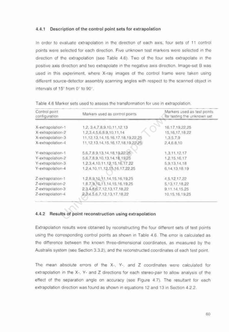
4.4.1 Oescrlpl10n 01 tile control point sets lor extrapolation
In orOOr to evaluale extrapolation In Ille direcllon oj each aXIs. loul selS 01 II conlrol
ponts were selected tor each d"ecl,on Five unknown test markers were selected on the
dlrachon 01 the ext rapolahon (see Table 4,6), Two 01 the lour sets exlrapolate In the
poSiti ve aXIs d,roction and two extrapolate in the negative aXI s dIrectIOn. tmage·set B was
used ,n thIS expe ro ment where X-ray Images 01 the contn)l Irame were taken USing
dillarent source·detector assembly scanning angles With respect 10 the scanned object m
Inte ..... als 0115 Irom 0 to 90
Table 4 6 Marker sets used to assess the IransforlMhon lor use m exlrapoiallOl'l
Contlo l po nt eont lpula~Ion
X·exuapolallon., X" xl,apolal10n·2 l(·u t,apolaltO!1·3 X·exuapolalion·4
y ·e ~lrapolallOn·'
Y·exTr~aTIOn·2
Y ·e. lrapo!atoon·3 Y ·,><lrapo!aTron·4
Z·'~!tapolabOn·l
7 ·,. trapolaTlOn·2 l·l!xlfllpolatlOn·3 l,ulrapola!IOf1·4
1.2. 3~.7.8.910. 1 '.1213
1.2.3.4.5.6.8.9.10, 11 ,14 I 1,12, 13. I~.15 16.17,18. 192225 , 1.1213.14, IS 16.17.18.1922.25
5,6.789,13,1418.19.22.25 5,6.7.8.9,10,13.14.18.19.25 1.2.3 ,4 .10.11 .12.15.16,1722 124.10, 11 ,12.15.16,17,22,25
I ,2.8,9 10.11 .14. I 5. 16, 19.25 , ,0.7.9.10.11. 14, 15. 16, 19.25 2.345.6.7.12.13,17,16.22 2.3 •• . 5,6.7,12. , 3.17. 18.22
4 .4.2 Results 01 point rl!'Construclion using extrapolat ion
MtI'~e's used as test po'rns 10' !e$!Jf19 the un~nown set
16.17. 19.22.25 15.16.17, 18.22 1.35.7,9 2.4.68.10
1.3.1 1 12.17 1.2.15,16.17 5.9.13.14,18 6,1413,1619
45.1217.22 5.13.17,111..22 9,11141525 10.15.16,19.25
£xltapolaaon results were obtaIned by reconstructUl{j the lour d!l:erenl sels 01 tesl ponls
usn'9 rhe correspondIng COl1trol pornts as shown In Table 01 6 The errOl IS C!llcuiated as
the dillerence betweon lhe kl1Ol'in Ihroe·dlmcnsoonal coordinates. !IS meaSl,lred by the
Austrahs system (see Seclron 3.3.2). and the r8OOf\Slructed coordinates of each lest potnt
The mean absolute errOl'S 01 the X-, Y· , and Z coord'nates were calculated to!'
e. trapola tlon In the X-. y. and Z directions lor each stereo-pair 10 allow analys!S 01 Ihe
ellect of the separallon angle an accuracy (see Fig\,a'e 47), The Issukanl tor each
eKlrapoiatlon dll8ClJon YlaS louncl as shown In eqll1l\lOflS 12 and 13 In Secl oon 4.2.2
00
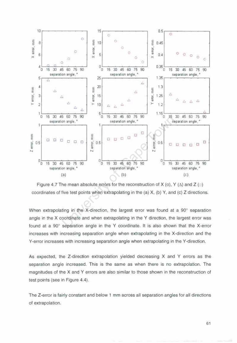
'",-----, , . i . , "
o
o
o
~O 15 3J 45 60 75 90
r-;::":·:":":'"::':':·'c"c'.· -l ' " , • ~ 1 > ,
! a 0 5 , "
.. pI .. ue" OI1gl. ,· ,.)
",-----,
,
r-:'~::":':'"::':':·'c"c'.· -l ~
•• ~.,>! ,." anglo. '
o 0 D a Cl [J
'01
!
""Oc-----.,
o 0 0 o ,
03S0C-'"'''~;;-".''m;;-;''''~;;-' . ...:"0-:":':'"::':-0"'0'.'_ ., , ~ ,
, "L.o-CO-"COo-~C:.J o 15 :JJ £5 60 75 90 "~" 01,'" ~"gIt.'
~ 0 5
" 00 15 JJ 45 60 75 90
.. " ... I,cn ."!Iit, • ",
Figure 4.7 The mean absolute errors for the reconstnJctjon of X (0). Y (to) and Z ('1 )
coordinates of ffve lest points whon exlrapolaling in lho (a) X, (b) Y, and (e) Z directions.
When extrapolating in the X·dir&Ctlon, tho largest error was found at a 90 ' separation
angle In the X coordInate and wnen extrapolating in the Y direction, tho largest error was
found at a 90" separa1ion angle in the Y coordinate. It Is also shown that the X-error
Increases w,rh increasing separation anglo when oXlrapoialing in tho X-direction and the
Y·olror increases with Increasing separation angle when eXirapoialing in the V-direction.
As expected. the Z-directlon extrapolalion yielded decreasing X and Y errors as lhe
separallon angle increased. This is the same as when Ihere is no extrapolalion. The
magnitudes of Ihe x and Y errors are also Similar to those shown In the reconstruction of
lesl points (see in Figure 4.4).
The Z-error is fairly COflstant and below 1 mm across all separation angles for al! directions
of extrapolaHon.
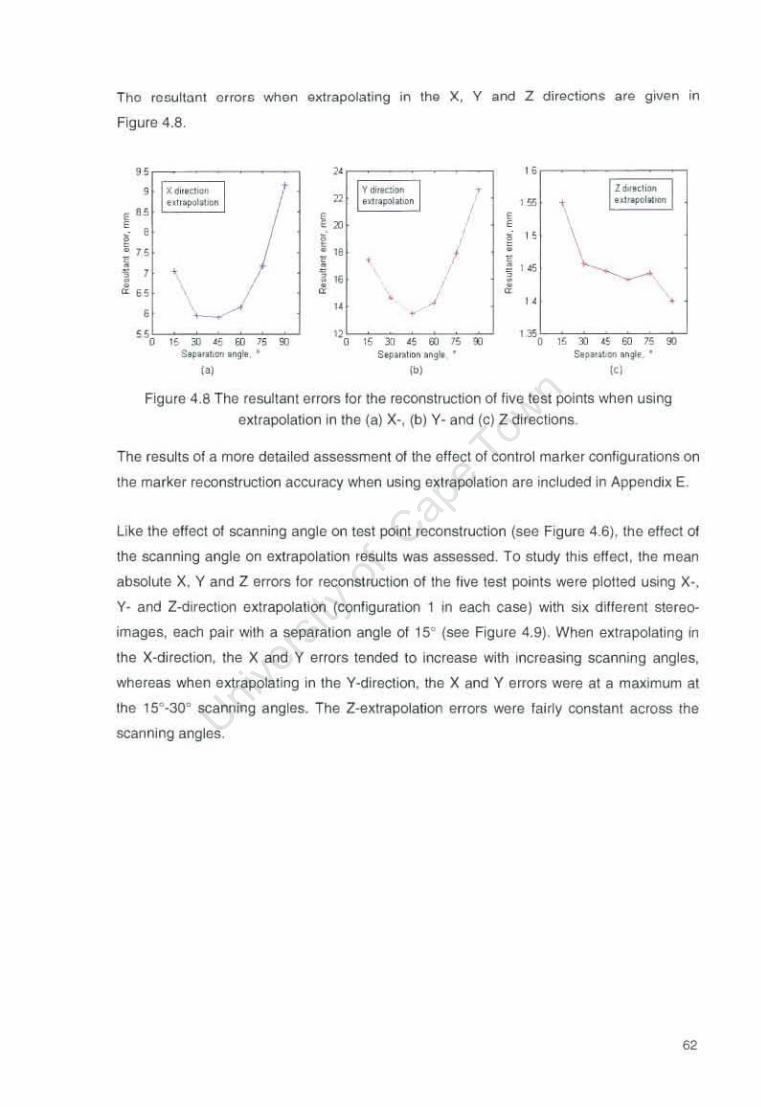
Tho .owlt"nl o'ro .. , whon e~t rapolatlng in the X. Y and Z directions aro g.ven ;n
FIgure 4.8.
"' ,.
" • 11:-'0- ·1 , § • lOOk . ... . ..,' ........ II . ,,' .......... ,. • .... .,,01 ...... ,"' I . !
\ • • i 1~ ! " I" I \.------
, , • , , , • I • , ,. '" "
, " ~ " • _ ....
", " • " • " • ", " • " • , • '", " • " • " • --... SOl'''''''''''''' . SO_ ..... .. jIr • ,., '" '"
FIgure 4.8 The resultaf1l errors for the reconstructiOn of live tast points when uSing
extrapolation In the (a) X" (b) y . and (cl Z directiOns_
The results of B more detailed assessment of !he eftect of control marker configurations on
the marker reconstruction accoracy wt1en using exlrapolatlon are included in Appendix E.
Uke the effect of scanning angle on test point reconstruction (see Figure 4.6), the effect of
the scanning angle on extrapolation results wa.s essessed. To study thiS ellect, the mea.n
absolute X, Y and Z errors for reconstruclion of the live lest points were plolted USing X'.
Y· and Z·direction extrapolation (configuration t in each case) with SIX di!lerent stereo
images, each pair with a separallon angle of 15° (see Figure 4.9). When eX1rapo!ating in
the X-di reClioo. the X and Y errors tended to fncrease with Increasing scanning angles,
whereas wtten extrapolating in the Y-diraction, the X and Y errors were a1 a mruomum al
the tS· ·30· scanning angles. The Z·extrapolation e.rors \WIre fairly constant across the
scanning angles.

e '" e , 0
., " • • '" ~ 0
• -0 ... 0 • 10 • <> 0 • • .A . • -' _. • 0 .15 , . ., ,"" ,"" 0'" ,'-",
Calm scann,ng .n~111 fo,m.,g th. 15" Up ... loon .. gle
"J e '50 e g 0
" '00 • • • 0 ., • • • 0 • • • , • 0 .15 .. ., "" ''''' "'75 ,..,
C'lfm StlMIIIg .ngln iormlllg ihe 15" sepilfillOn angle
(bJ , , , ,
15 .~. , .. -- --·· -A· .. • • • • > 0 • o. -_ ..... -0 ' n 05 I> 0 ---9.
0 .... . .. o · . __ . • " .. ~ 0
0 .15 .. ., '"" ."" "'75 ,..,
C·."" .ealVWlg angle$ fonTnng !he 15" soop,uallOO Xlgla
'<J F>gure 4 9 An lIIuslrabon oIlhe elfecl 01 C·arm scannIng angles lhal lorm the separahon
angle 01 1 S· on the X (ol,Y (.1) and Z (0 ) mean absolute errors when extrapolating In Ihe (a) X· (b) y. and (e) Z.orecttons
To SIMT1marise, the errors obsefVed men reconstructing lesl !>Onts using eJ(lrap~allOn
were mudllarger lhan when the Iesl points are well-.distribuled around the contrOl space.
n was also shown that the extrapolation errors depended on separatIon angle, S(:ann,ng
angje end the conl igUfIUIOI1 01 control and tesl points

4.5 Reconstruction of phantom points using interpolation
The purpose ot thIS experiment is 10 assess the usc of Statscan using Interpolatioo (i.e.
reconst ructl()(1 ot un~nown points trlat lie within Ihe volume dellmlled by lhe contrOl POlnIS)
A phamom with measured object marker positions (see SeellOn 342) was Imagod WIthin
the calibralJon Irame (see FlgUie 4.10) using differenl source-detector assembly scanning
angles with respect to tile scanned object In Imervals of 15 Irom oe to 90' (Image-set B)
Figure 4.1 0 The phamom with in the calibration Irame on the patient tab le of the Statscan
machine. Groote SChuur Hospital
As in prevIous experiments. the X·ray images taken at seven dilterent scanning angles
(0 . t5 , 30', 45, 60 , 75~. SO<) were paired to form 21 combinations at SIX dlfterem
separat ion angles. An example of a stereo-pair 01 Statscan Images taken al scanning
angles of 0 and 45 (45 separation angle) is given in Figure 4 11

Figure 4 11 A pair oj Statscan Images where the phantom was uKhographed WIthin the
catibratlOn frame at 0 ancl 45 respec1lVeI~
The Matlab routines were used to identll~ the two·dimenSlOl1al (l . ~ ) cOOfdlfla tes 01 the
calibratlOl1 markers (soo SectlOl1 34 t) and phantom markers (see Section 3 4 2) on each
Image The manual correctlOfl of calibratloo frame markers for lmage·set B (see Table 4 II
applies hele AegardorlQ the phantom markers, at cenaln C·arm angles 11 was di" rculltO be
absolutely sure whether the marker label was identified correr::tl~ and also whether the
c€Iltre was Identrfled C()(rectl~ b~ the Matlab program tn cases wf"oere thE; marker label
Idenlifrca tlOl1 was sure but the marker was overlapped b~ other markers or Perspex
columns. the marker posl!lOfl was manually COfrected (see Table 4 7) In cases where
there was COl"IluslOfl 01 marker label rdentdicatron or where the marker was completely
occluded b~ some obteC1 (e,g Perspex column). the marker was excluded. ThIS study dJCI
OOt establish an IdentdrcatlOl1 routine lor occluded marker.;. such as thaI presented by
Kaptelll ef al .. 2005
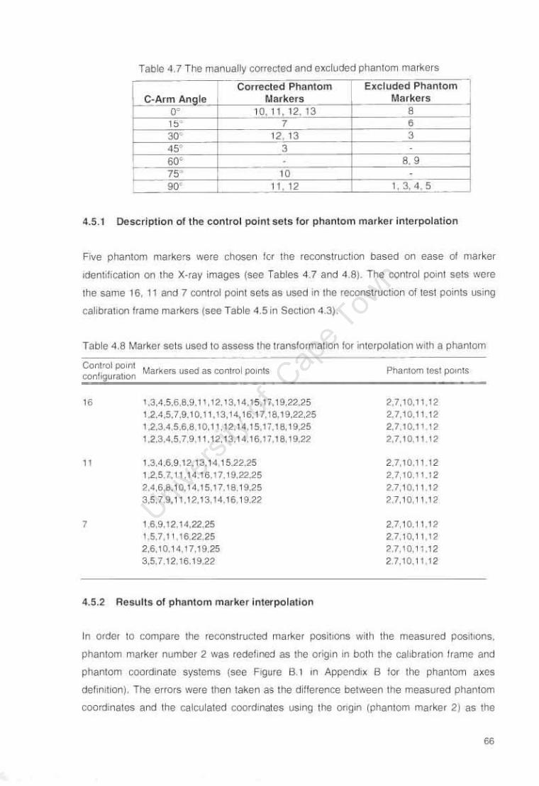
Table 4.7 The manually corrected and excluded phanlom markers
, .
4.5 .1 Description of the contro l point sets for phantom marker interpolation
Five phanlom markers lIIere chosen fer the reconstruction based on ease 01 marker
Idenllflcation on lhe X·ray images (see Tables 4.7 arld 4 8). The contro l poll1t sels IVere
the same 16, 11 and 7 col1trol point sets as used 111 the reconst ruction of test paints using
cal Ibration Iramo markers (see Table 4.51n Section 4.3),
Table 4.8 Marker sets used to assess The translormallOI1 for interpolatron With a phantom
COn!.01 poInt confIguratIOn
"
,
Markers used as control points
I .3.4.5.6.B.9. I I, I 2. I 3,1 4. I 5, I 7, I 9,22,25 1.2.4.5.7,9.10. I I , I 3. I 4. itS. 17, I 8, 19.22.25 1.2.3.4,5.6,8. I O. I 1.12.14,15, I 7. I 6, 19,25 1.2,3.4.5.7,9. I 1. I 2. 13, 14.16. 17. I e, I 9,22
1.3.4.6,9.12. I 3, 1 4, 1 5.22.25 1,2.5 7, 11.14.1 6. 17. 19.22.25 2.4.6,8. 10, 14, IS, I 7. 1 8. 1 9.25 3,5 ,7.9.1 1,1 2,13,1 4,16,19,22
1,6.9,12.1 4,22.25 1,5.7,11 16.22.25 2,6.10.14,17,19.25 3.5.7.12,16.19.22
4.5.2 Results of phantom marker interpolation
2,7.10,1 1,12 2,7.10,1 1.12 2,7,10.11 .12 2.7.10,11,12
2,7.1 0.1112 2,7,10.1 1.1 2 2.7, 10.1 112 2.7.10,11.12
2,7, 10.1 1,1 2 2.7.10.11 ,12 2.7.10.11,12 2.7.10,11,12
In order to compare the reconst ructed marker positrons w~h the measured POSitIonS,
phantom marker number 2 was Jedefllled as the origll1 in both the ca llbrallon trame and
phantom coordlnato systems (see Frgore B. I III AppendIX B for the phanlom axes
defll1ll1on). The errors were then laken as the difference between the measured phantom
coord,nates and the ca lculated coordmates using the Ol<gln (phal1tom marker 2) as the
"
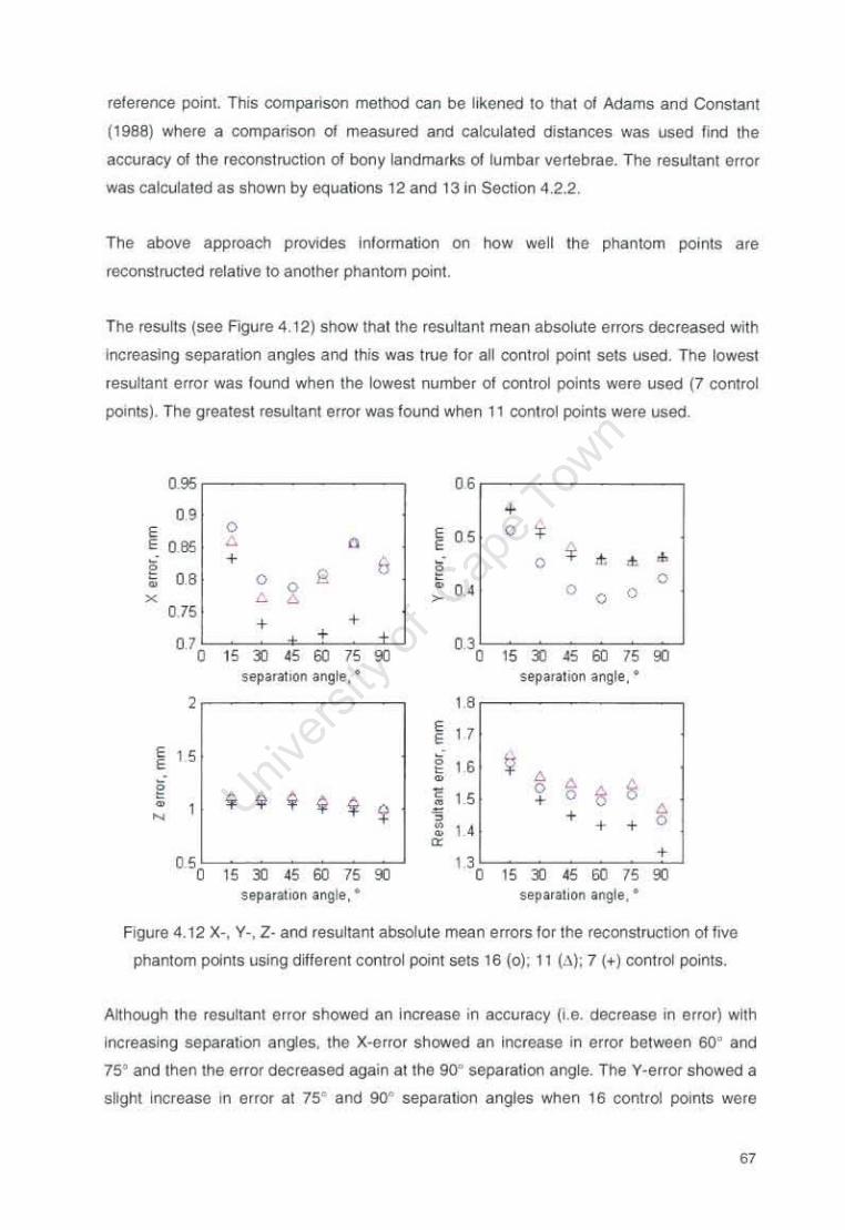
relerence pornt. This comparison method can be likened 10 that 01 Adams and Constant
(1968) where a comparison 01 measured and calculaled dlslancBs was used fiocl Ihe
accuracy oIlhe re<:onslruclion 01 bony landmarkS 01 lumbar vertebrae. The resultanl error
was calculated as shown by equations 12 and 13 in Section 42.2.
The above approach provides Information on how well the phantom points are
reconstructed relative to anolher phantom poijnt.
The resulls (see Figure 4.12) show that the resultanl mean absolule errors decreased with
Increasing separallo-n angles aocl this was tll.le for all control point sets used. The lowest
reSllltanl error was loulld when the lowest number of control points were used (7 control
pOints). The greatest resultant error was found when 11 control poinlS were used.
0.95 0.6
09 + E 0 ,OS 0 ~ E 0.85
, a ~
~ + 6 ~ 0 .+ • •
" 0 2 0 0 -co 0 0 x L 0 > 0
075 + + 07
0 + 03
0 " lJ " 60 " '" " lJ " 60 " '" separat<on ang le,' separallOn ~nQle, • , " E
" E , IS g " ~ g • , a e ~ $ 9 E IS
0 0 8 • ~ • ~ • + a x + N • 0 • + + • " • "0 "0
+ 15 lJ 45" 75 '" " lJ 45 60 75 '" separaliOn angle. ' separat.on angle .•
Figure 4.12 X-, yo . Z- and resultant absotule mean errors for the reconstruction of /rve
phantom points uslng d~ferentcootrol point selS 16 (0); It (;'II ; 7 (+) control points.
AHhough the resultant erlOl showed an Increase In accuracy (I.e. decrease In error) with
Increasing separatlOO angfes. the X-error showed an increase in error belween 50' and
75' aM then the error decreased again al the 90" separatioo angle. The V-errOl shoWed a
slight Increase In error at 75' and 90' separation angles when 16 COf'ltrol pomts were

used. however this increase In Y·error was not as pronounced when using 11 and 7
control points.
Another nOleworthy ooservabOllls thallhe lowest X" Z· and resultant errors were loond
when usmg 7 control points. howeV8f the lowest Y·error was lound when using 16 control
pawliS.
While the mean absolute erTOfS IOf the Z COOfdinales were tugher than thOse seen in
previous eKPSrimenls, the error was constant across aN separation angles and control
point conf'9Ura tlOr"ls. The three..oimer\SlOl"lal rllOOl"lS\fVCtlOfl 01 live phanlom points WIthin
the calibralion frame IS sho¥rTI graphlcaDy in F9Jffl 4.13.
" ,22 25- 6
" ". ,, _ x "" 18 ,
0 I ..
" 8 , 600 S " 6
~ 0 0
.100 \I' " Dl ,.
I '
100 0
Y ·100 ·100 l
Figure 4. 13 A three-dimensional plol 01 the 251rame marker measured posItioos (~), t I labened control po4nlS ( ... ) and the 5 interpoteted points (0) 'Mtl'in !he calibration frame
space.
To summarise. resultant mean absolute errors 01 beTWeen 1.33 mm and I 64mm were
observed when reconstructing unknown potnts using interpolation (p0."ts I,e Within the
conlrol point space). The errors were shown to depend on separation angle and number of
control polms.
"
Chapter 5: Discussion
The results obtained from the experiments presented in Chapter 4 highlight differences in
the three..<Jimensional reconstruction of discrete points when the reconstruction is
performed under various conditions such as varying separation angles and numbers of
control points. Point reconstruction errors when using interpolation and extrapolation
marker configurations have also been established.
In this chapter, these results are compared with those of previous stereophotogrammetry
studies where projective transformation techniques such as the DL T method were used.
Some Roentgen Stereophotogrammetric Analysis (ASA) results are used for oomparison
where relevant. In addition, the results are compared to those of previous Statscan point
IocaUsation experiments (Dou~as st al., 2004).
While many of the findings agreed with the literature results, several noteworthy
differences were observed. The differences between the results of this study and those in
the literature are discussed in detail in this chapter and possible reasons for the
differences are examined.
The material used in this study differs from that used in the literature and these differences
may account for differences in results. The set-up of equipment used in this study is
therefore compared to that of the literature to assess the impact the differences could have
on reconstruction errors (see Section 5.1).
In addition, the effect of different calibration configurations 'On reconstruction accuracy has
been compared to that described for previous studies. Despite the fact that the marker
configurations and separation angles differ from those used in the literature, the
comparison is useful since trends in reconstruction accuracy can be identified {see Section
5.2).
5.1 Equipment as a Possible Source of Error
5.1.1 The Calibration Frame
This section analyses the calibration frame as a possible source of reconstruction error.
69
While sturdy, the calibration frame was not completely rigid. If a force was applied to the
frame, it tended to bend slightly before returning to its original shape. Any errors that may
have been introduced through slight altering of the control frame were considered
negligible. The maximum standard deviations for the measured marker coordinates were
0.10 mm, 0.12 mm and 0.06 mm, respectively in the X-, Y-, and Z-directions (Section
3.3.2) and this is in line with the measurement accuracies of previous studies e.g. 0.5 mm
accuracy for measurement with a Theodolite, Chen et al. (1994).
The markers on the calibration frame were 10 mm in diameter, which is large in
comparison to those used in other X-ray stereophotogrammetry studies (0.7 mm in the
Andre et al. (1994) st4dy; 1 mm in the Plamondon and Gagnon (1991) study and 3 mm in
the Choo and Oxland (2003) study). However, in a conventional stereo-photogrammetry
stUdy, 3.18 cm markers were used (Chen et al., 1994) and in a conventional
cinematography study, 3 cm spherical markers were used (Hinrichs and McLean, 1995).
The large markers could have introduced measurement errors, although the comparisons
shown in this study are relative and thus the overall results of trends should not be
affected.
As in the study of Chen et al. (1993), a limitation of this study was that the calibration
frame markers were fixed. The marker positions could not be altered once they were glued
in place, even when it was found that several calibration frame markers overlapped one
another in the images. It would have been prudent to perform a test with the frame before
the markers were finally glued into position.
In such cases where the calibration markers overlapped on the X-ray images, the marker
centres were estimated manually using the Matlab pixel value and zoom functions. This is
expected to have a minor impact on errors since the manual marker identification standard
deviation was found to be 0.08 mm and 0.07 mm for x and y image coordinates
respectively compared to 0.09 mm and 0.02 mm for x and y image coordinates
respectively for marker correction using the Matlab program. Where markers coukl not be
identified on the stereo images, these markers were completety excluded from the
experiments.
Although the calibration frame was designed to avoid object truncation, (see Section 3.3.1)
insufficient margin was included in the design geometry to take changes in patient table
set-up into account. This lead to marker truncation in image-set B. Despite this, sufficient
remaining calibration frame markers were available to perform the required experiments.
70

5.1.2 The Digital Imaging System
While the sources of error inherent to the process of Statscan digital X·ray image
generation were not studied in detail, possible sources of error are mentioned based on
observations when using the X·ray scanner.
The Statscan X·ray imaging syste'm is different to those used in other studies because It is
a fully digital system while many of the studies reviewed in the literature were based on
film or digitised X·ray film.
The geometry of the Statscan machine is also different to the X·ray machines used in the
literature. The Statscan machine has been designed for clinical use and therefore has a
movable patient table. This table, which can be raised and lowered, had to be raised for
the duration of the image pair acquisition so that the C·arm could be rotated. However, the
table does not have a height measurement and so it was not possible to be confident that
the experiments performed with imaga.set A and B were performed under exactly the
same conditions.
The fact that it was not possible to position the calibration frame within the X-ray beam for
all scanning angles in imaga.set B demonstrates that there were some set-up differences.
This led to the exclusion of four markers (20, 21, 24 and 25) that could otherwise have
been used in the study. Since these markers were unavailable, the experiments could not
make use of the same control point sets as were used in the previous Statscan
stereophotogrammetry study of Douglas st al. (2004).
The table and calibration frame positions were not altered in any way between X-ray scans
to ensure that they remain as a rigid unit, otherwise, the transformation parameters would
be invalidated (Adams, 1981). Therefore, no errors were introduced in this way.
The accuracy of the C-arm angle measurement is not known but errors in the scanning
angle would not affect the trends reported. On the other hand, if it was necessary to
calibrate the system prior to using the system for patient studies i.e. radiograph the patient
without the calibration frame (Adams and Constant, 1988), the fact that the Caarm may not
return to exactly the same point each time would probably lead to significant
reconstruction errors.
71

The accuracy of the scanning start and end point settings is also not known. The start and
finish positions should be the same for each image so that the image y-coordinates are not
significantly offset from one image to another. The Z-coordinate was determined by taking
the average from both stereo-images so the offset should not significantly affect the
reconstructed Z-coordinate accuracy.
The limitation of the Statscan machine is that the C-arm has a limited 90° rotation. This
limited the angles that were used in the experiments.
5.2 "rhe effect of calibration variables on reconstruction accuracy
5.2.1 The reproducibility of two-dimensional marker identification
The identification of marker centroids plays an important role in the three-dimensional
reconstruction of discrete points (Adams and Constant, 1988); therefore the reproducibility
of marker identification was evaluated. The literature presents two main ways of assessing
marker identification accuracy by either the comparison of the two-dimensional
coordinates obtained by different methods (Wang et BI., 1996; Ostgaard et BI., 1997), or
the comparison of reconstructed three-dimensional coordinates that were found using two
dimensional image coordinates obtained by different methods (Ostgaard et al., 1997;
Douglas et BI., 2004). As in Ostgaard et BI. (1997), both of these methods were used in
this study.
In the present study, the mean standard deviations for the eighteen sets of two
dimensional coordinates (nine selections on each 0° and 90° image) using the marker
centroid correction program were approximately 0.09 mm and 0.02 mm for x and y image
coordinates respectively (estimating 0.2 mm per pixel). These errors are significantly
larger than the errors reported in the literature, 0.007 mm to 0.008 mm (Ostgaard et BI.,
1997) and 0.013 mm to 0.057 mm (Wang et BI., 1996). This can be attributed to the fact
that the markers used in this study (10mm) were more than a factor of 10 bigger than
those used in the referenced studies, 0.8 mm (Ostgaard et BI., 1997) and 1 mm (Wang et
BI., 1996). It may be possible to identify a marker centroid on a smaller marker to greater
accuracy. The fact that the error is greater in the image x direction could be attributed to
the marker elongation in the x-direction, so there is a greater chance that the centre in the
x-direction could be poorly identified.
72
While the reproducibility of the two-dimensional marker centroid identification is relatively
low in this study, the marker centroid correction program results are comparable to the
standard deviation for typical manual marker centre identification, 0.05 mm (Wang 8t al.,
1996). In addition, the results obtained for manual marker selection of the same markers
(0.08 mm and 0.07 mm standard deviation for image coordinates x and y respectively,
estimating 0.2 mm per pixel) are also similar in magnitude to the results reported by Wang
at al. (1996).
The mean standard deviations for the reconstruction of the nine sets of 15 manually
identified markers were 0.05 mm, 0.07 mm and 0.05 mm for X, Y and Z-coordinates
respectively. When using the marker correction program, there was only a slight reduction
in error (0.07 mm, 0.06 mm and 0.02 mm for X, Y and Z-coordinates respectively). The
results were similar to those found by Douglas at al. (2004), where standard deviations of
0.14 mm, 0.06 mm and 0.05 mm were reported for the X, Y and Z directions respectively.
The three-dimensional reconstruction reproducibility was significantly lower than that found
by Ostgaard 8t al. (1997) in an RSA study, where standard deviations of 0.005 mm to
0.006 mm were obtained. However the results were within the region of magnitude found
by Gussekloo at al. (2000) where 0.12 mm standard deviation was obtained in each
direction. In addition, the res.ults are comparable to the reproducib~ity of the automated
RSA procedure by Vrooman at al. (1998), where translation errors between 0.03 mm and
0.11 mm were reported.
Differences in two-dimensional marker coordinates between this and other studies .could
also be due to differences in image resolution.
While a lower error in locating the two-dimensional marker centroids is desirable since it
reduces the magnitude of the reconstruction errors, it will not change the relative effects of
the mathematical algorithm and marker distribution (Choo and Oxland, 2003). Therefore,
the relative effects of separation angles and control point configurations on reconstruction
accuracy can still be compared.
5.2.2 The effect of separation angle and scanning angle on reconstruction
accuracy
The results from the reconstruction of control pOints (image-sets A and B), test points
(image-set B) and independent phantom points found by interpolation (image"'S8t B)
73
showed that the resultant mean absolute errors decrease with increasing separation
angles irrespective of the number of control points used (see Figures 4.2, 4.3, 4.4 and
4.12). This result agrees with previous stereophotogrammetry studies (Wood and
Marshall, 1986; Adams and Constant, 1988; Plamondon and Gagnon, 1991; Douglas et
a/., 2004).
The improvement in accuracy with an increase in separation angle can be attributed to the
fact that more information is available about the object space when the stereo-pair is taken
at large separation angles. Adams and Constant (1988) pointed out that small
misidentifications on the two dimensional images will result in significant differences when
small separation angles are used, but that these errors would be minimum in biplanar
radiography, where a goo separation angle is used. This explains why the biplane
radiography method is popular in X-ray stereophotogrammetry.
Comparing the results with those from Douglas et a/. (2004) where a similar study was
performed with Statscan using different control point sets we notice that for control and
test point reconstruction the maximum X and Y errors are found when using a 15°
separation angle. In contrast, the results from the reconstruction of test pOints using
extrapolation did not demonstrate an increase in accuracy that corresponds to an increase
in separation angle. This will be discussed in Section 5.2.4.
In the reconstruction of control pOints, the mean absolute Z-error was fairly constant
across all the separation angles: in the region of 0.5 mm for image-set A and 0.4 mm for
image-set B. In the reconstruction of test points, the mean absolute Z-error was also found
to be constant across all separation angles in the region of 0.5 mm. This can be attributed
to the fact that the Z coordinate was found by the linear mapping of the image y
coordinate. -rhe results agree with those of Douglas et a/. (2004), where the mean
absolute error in the Z direction was constant between 0.4 mm and 0.5 mm, depending on
the number of control points used.
The slight upward trend in mean absolute Z-error with increasing separation angle could
be attributed to possible marker centre identification errors present in some markers that
were used in the reconstruction. This is supported by the results in Figure 4.5 where the
test point reconstruction was performed for four different marker configurations of 16
control points each. The graph shows an increase in Z-error in configurations 1 and 2,
whereas the Z-error is fairly constant in the other two reconstructions.
74
The results from the different configurations cannot be compared to the different
configurations of Challis and Kerwin (1992), since the calibration frame used in the present
study has a different shape, and the markers are not arranged symmetrically.
The effect of the scanning angle orientation on test point reconstruction accuracy was
assessed using a constant separation angle of 150 t as was used by Plamondon and
Gagnon (1991). A significant difference in the V-direction was found with large errors
found at larger scanning angles. This can be explained by the fact that the caltbration
frame was not symmetrical and therefore despite the constant separation angle used, the
information available for the generation of transformation parameters was different at
different scanning angles. These results agree with Plamondon and Gagnon (1991), who
observed similar significant differences (0.12 mm mean compared to 0.04 mm mean) in
the x-direction (equivalent to our V-direction) when a higher film angle (equivalent to our
scanning angle) was used.
5.2.3 The effect of the number of control points on reconstruction accuracy
The results from the reconstruction of control points (image-sets A and B) show that the
mean absolute error is highest when high numbers of control points are used (21 points)
and the accuracy increases with decreasing numbers of control points. The lowest mean
absolute errors were seen in the reconstruction of 7 control points. This result agrees with
the findings of Challis and Kerwin (1992), Hinrichs and McLean (1995) and Douglas et al.,
(2004). While the magnitude of the reconstruction errors are shown to be much lower than
those of Hinrichs and McLean (1995), the results are comparable to the mean errol'S of
Adams and Constant (1988) for the reconstruction of 21 control points (0.3 mm, 0.3 mm,
0.9 mm in the X, V and Z directions respectively).
Like in the Statscan study, in the cinematography study of Hinrichs and Mclean (1995),
with a 900 separation angle, the highest accuracy was seen in the reconstruction of the
lowest number of control points (16 control points in this case) and errors in reconstructing
control points increased as numbers of control points were increased (16 to 60 control
points).
In contrast, when the test points were reconstructed, the mean absolute error was highest
when the smallest number of control points (7 control points) were reconstructed (see
Figure 4.4). This is in agreement with the results of Challis and Kerwin (1992), Wood and
Marshal (1986) and Hinrichs and McLean (1995). In a study for minimally invasive hepatic
75
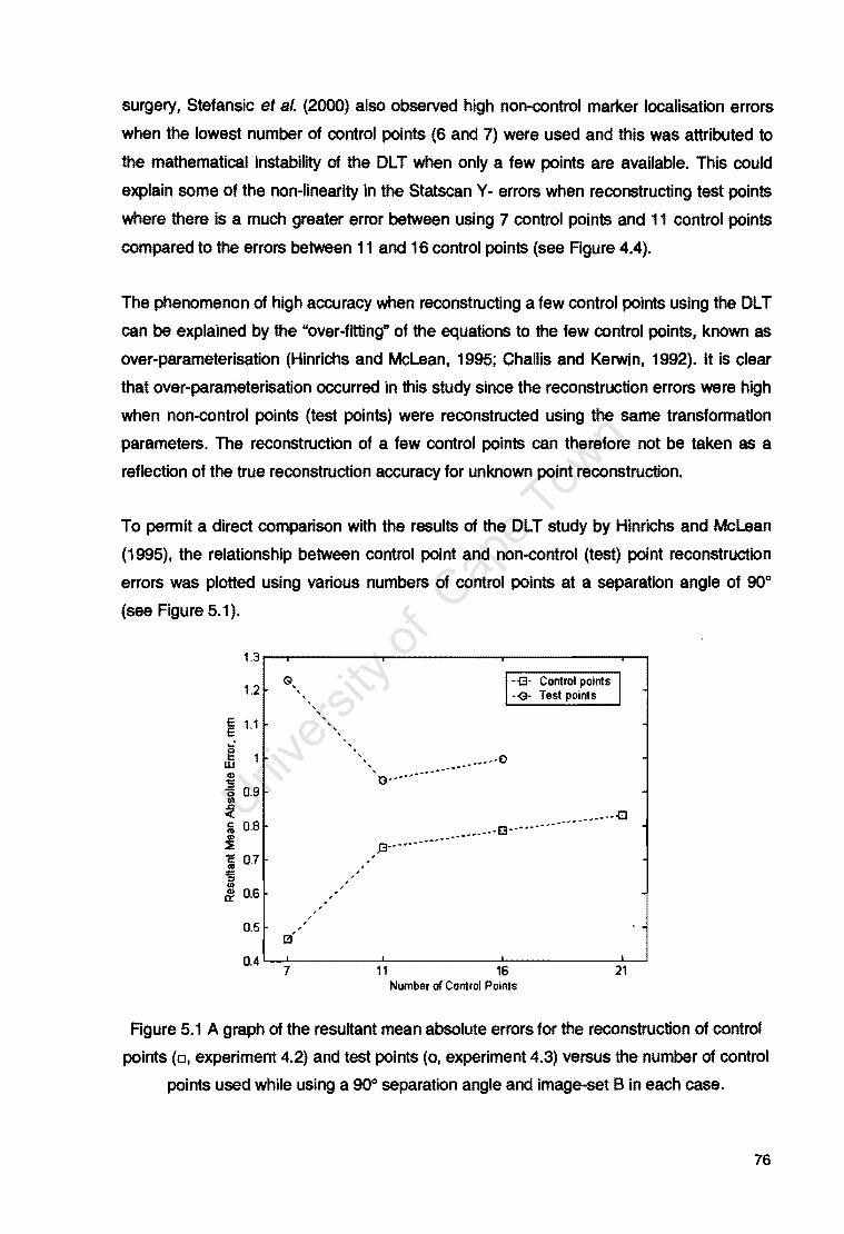
surgery, Stefan sic et al. (2000) also observed high non-control marker localisation errors
when the lowest number of control points (6 and 7) were used and this was attributed to
the mathematical instability of the DL T when only a few points are available. This could
explain some of the non-linearity in the Statscan Y - errors when reconstructing test points
where there is a much greater error between using 7 control pOints and 11 control points
compared to the errors between 11 and 16 control points (see Figure 4.4).
The phenomenon of high accuracy when reconstructing a few control points using the DL T
can be explained by the "over-fitting" of the equations to the few control points, known as
over-parameterisation (Hinrichs and Mclean, 1995; Challis and Kerwin, 1992). It is clear
that over-parameterisation occurred in this study since the reconstruction errors were high
when non-control pOints (test points) were reconstructed using the same transformation
parameters. The reconstruction of a few control points can therefore not be taken as a
reflection of the true reconstruction accuracy for unknown point reconstruction.
To permit a direct comparison with the results of the DLT study by Hinrichs and Mclean
(1995), the relationship between control point and non-control (test) point reconstruction
errors was plotted using various numbers of control points at a separation angle of 900
(see Figure 5.1).
1.3....-.,..------.-------,--------,r----I
1.2
~ 1.1
g 1 w CD 'S 15 0.9
411
~ i O.S ~ ; 0.7 -s (I)
t'i 0.6
0.5
G"
[~" ,
, ,
, , ,
1--G- Control points I -~ Test points
'''', ~~~ .... E> " G··· .. ----···----
• _ -£3 ___ • __ -. ---- ---. --- --l!l .... " .. -... -....... -• .13------
.
0.4 '--7.1------'-'-,-----' .... 6------'2'---'
Number of Control Points
Figure 5.1 A graph of the resultant mean absolute errors for the reconstruction of control
points (0, experiment 4.2) and test points (0, experiment 4.3) versus the number of control
points used while using a 900 separation angle and image-set B in each case.
76
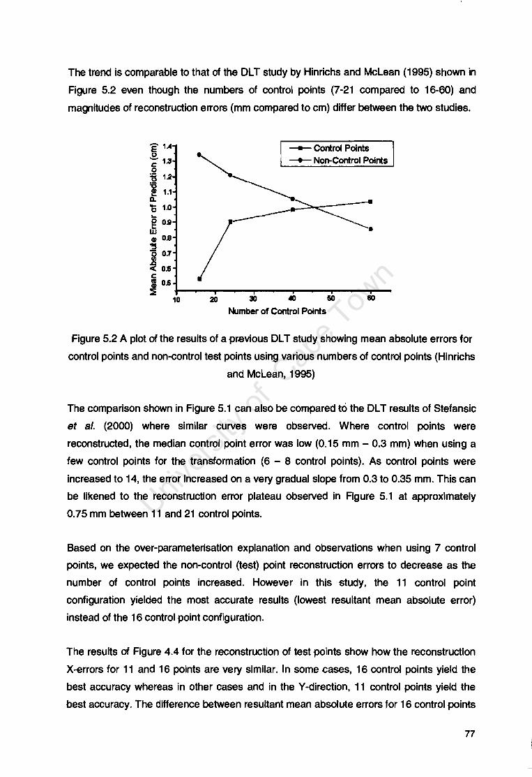
The trend is comparable to that of the DL T study by Hinrichs and McLean (1995) shown in
Figure 5.2 even though the numbers of control points (7-21 compared to 16-60) and
magnitudes of reconstruction errors (mm compared to cm) differ between the two studies.
S1A --- Control Points u ~ 1.3 ---.- Non-Control Points 0 13 1.2 '6 ~ 1.1
D.. b 1.0 ... g0.9 w • CD 0.8 '5 i 0.1
~ 0."6 c II 0.6 ::E
10 ~ ~ ~ ~ m Number of Control Points
Figure 5.2 A plot of the results of a pravious DL T study showing mean absolute errors for
control pOints and non-control test points using various numbers of control points (Hinrichs
and McLean, 1995)
The comparison shown in Figure 5.1 can also be compared to the DL T results of Stefan sic
et a/. (2000) where similar curves were observed. Where control points were
reconstructed, the median control point error was low (0.15 mm - 0.3 mm) when using a
few control points for the transformation (6 - 8 control points). As control points were
increased to 14, the error increased on a very gradual slope from 0.3 to 0.35 mm. This can
be likened to the reconstruction error plateau observed in Figure 5.1 at approximately
0.75 mm between 11 and 21 control points.
Based on the over-parameterisation explanation and observations when using 7 control
pOints, we expected the non-control (test) pOint reconstruction errors to decrease as the
number of control pOints increased. However in this study, the 11 control point
configuration yielded the most accurate results (lowest resultant mean absolute error)
instead of the 16 control point configuration.
The results of Figure 4.4 for the reconstruction of test points show how the reconstruction
X-errors for 11 and 16 points are very similar. In some cases, 16 control points yield the
best accuracy whereas in other cases and in the Y -direction, 11 control points yi~d the
best accuracy. The difference between resultant mean absolute errors for 16 control points
77
and 11 control points when reconstructing test points is less than 0.1 mm, which may be
within the random error region, thereby explaining the highest accuracy observed when
using 11 control points.
An improvement of test point reconstruction accuracy with the use of an increased number
of control points is also explained by Chen et al., 1994 as being due to the likelihood of a
more even distribution when an increased number of control points are used. The
configuration of the control points could therefore also have an effect on the accuracy.
This is illustrated in Figure 4.5 where different errors were observed when different
configurations of the same number of control points (16 control points) are used to
reconstruct the five different test points across different separation angles. One can clearly
see the difference in error that is purely as a result of configuration. Chen et al. (1994)
states that it is generally accepted that it is more important to have well-distributed control
points than just to increase the number of control points. While every effort was made to
ensure even distribution of control points in the experiments, the inherent uneven
arrangement of control points on the calibration frame may have introduced errors.
In addition, the higher error that is seen when a minimum number of control points are
used to reconstruct test points can be explained since the transformation parameters are
more vulnerable to the individual random error of the control points (Chen et al., 1994).
Chen et al. (1994) reported an increase in DL T accuracy as the number of control points
increased from 8 to 16, but found that the accuracy did not continue to increase when
numbers of control points exceeded 16. The results of Hinrichs and McLean (1995)
dispute this since their results showed a continued increase in accuracy beyond 16 points
to the maximum number available (60 control points). The reason given was that while
Hinrichs and McLean (1995) reconstructed the same test points for each DL T assessment,
Chen et al. (1994) did not.
Although the same test points were reconstructed for each of the 16, 11 and 7 control
points, the present study did not include as many control pOints as Hinrichs and McLean
(1995), where as many as 60 control points were available. It was therefore not possible to
establish whether there would be a continued improvement in test point accuracy if more
than 16 control points were used, as demonstrated by Hinrichs and McLean (1995), or
whether the accuracy would reach a plateau if more than 16 control points were used.
78

5.2.4 The reconstruction accuracy when extrapolating
As expected, the errors resulting from discrete point reconstruction using extrapolation in
the X and Y directions were found to be significantly larger than those for the
reconstruction of well-distributed test points on the calibration frame. This is in line with the
finding by Wood and Marshall (1986) and Hinrichs and McLean (1995) that unknown
points should lie within the volume defined by the control points for optimum DL T
reconstruction.
The highest errors were found when extrapolating in the V-direction, where the X-error
was highest at a 150 separation angle (13 mm), and the V-error was highest at a 900
separation angle (22 mm). It was expected that the V-error should be the greatest since
the least spatial information is available in the direction of extrapolation. The same
phenomenon was found when extrapolating in the X-direction, where the X-error was the
greatest of the three coordinate errors (9 mm at 900 separation angle).
When examining the reconstruction of each individual control point configuration, it was
shown that the error tended to be greatest when the test pOints were furthest away from
the control point volume (see Figures E.2 and E.3 in Appendix E). This result agrees with
that of Hinrichs and McLean (1995) and Choo and Oxland (2003), where the accuracies of
different levels of extrapolation (distances from the control points) were assessed. Hinrichs
and McLean (1995) found that at maximum extrapolation (expressed as 300%), the errors
had increased nearly ten-fold compared to the 0% condition (6.01 cm compared to
0.61 cm). While Choo and Oxland (2003) found that accuracies were better if an initial
DL T calibration was done followed by calibration frame removal compared to extrapolation
accuracies. In addition, Wood and Marshal (1986) found that the errors were between
50% and 100% greater than reconstruction errors when using well-distributed control
points.
On further examination of the reconstruction of each individual configuration, it was also
observed that the extrapolation configuration played an important role in reconstruction
accuracy. This is best illustrated by the mean absolute errors when extrapolating in the
X-direction (see Figure E.1 in Appendix E). The errors for configuration 1, where the
control pOints were grouped at the bottom of the frame and the test points were grouped at
the top, were considerably larger than those for configuration 3, where the control points
were grouped on the top of the frame and the test pOints were at the bottom (see Figures
E.1 and E.2 in Appendix E). This could in part be due to the distance of the test points
79

from the control points (they were further apart in configuration 1), but this could also be
due to more information being available in the X-direction when using configuration 3.
The results of the extrapolation study are different to those of Douglas at al. (2004) , and
this is attributed to the fact that, while Similar, the control and test configurations are not
the same. Douglas at al. (2004) showed that the resultant X-direction extrapolation error
first decreased from 48 mm to below 5 mm through separation angles of 15° to 60° and
then increased to above 5 mm at a 90° separation angle. The present study results also
showed an initial decrease in X-extrapolation resultant error followed by an increase (see
Figure 4.8), however the error magnitudes differ somewhat (7 mm to 6 mm through
separation angles of 15° to 45° followed by an increase to 9 mm at a 90° separation
angle). The difference in error magnitudes has been shown to depend on control and test
marker configuration; therefore it is assumed that this is the reason for the differences
between the present study results and those of Douglas at al. (2004).
In the present study, the resultant mean absolute errors for V-direction extrapolation were
shown to first decrease from 18 mm to 13 mm through separation angles 15° to 45°, and
then increase to a maximum at 23 mm at a 90° separation angle. In contrast, Douglas et
al. (2004) found that the resultant V- error decreased conSistently from 14 mm to 6 mm as
separation angles were increased from 15° to 90°.
These V-direction extrapolation results can be further compared to those of the Wood and
Marshall study (1986). Taking X-ray source and image orientations into account, we can
equate the Statscan X, V and Z coordinate system to the Wood and Marshall (1986) Z-,
X-, and V coordinates and so using the Statscan coordinate system we can say that the
Wood and Marshal (1986) extrapolation was in the equivalent V direction. It was found that
the highest extrapolation reconstruction errors were also found in the V direction,
supporting the results of the present study. In addition, Wood and Marshal (1986) showed
that the V-errors were higher with increasing separation angles (13.1 mm with a 45°
separation angle, 13.5 mm with a goo separation angle). The mean resultant errors were
also found to be higher when the larger separation angles were used.
The results from V-direction extrapolation also showed an unexpected increase in Z-error
with increasing separation angle. This was unexpected Since the Z-error was merely a
linear mapping of the y-image coordinate. The error is attributed to the cumulative effect of
relatively poor two dimensional coordinate localisation in markers that were furthest away
from the detector banks, as well as slight image distortion. This can be justified since the
80

set of control points chosen in V-direction extrapolation were either very close to the
detector bank or far away from the detector bank. The resulting relatively poor two
dimensional coordinate localisation of control points could have resulted in poor
reconstruction of the test point Z-coordinate when large separation angles (which use
laterally scanned images) were used. To reinfor~ this theory, we plotted the Z- mean
absolute errors from V-direction extrapolation when reconstructing five test points using 11
control points (configuration 1) and a 15° separation angle The Z-errors are plotted against
the six pairs of scanning angles that were used to obtain the stereo-images {0° and 15°,
15° and 30°,30° and 45°,45° and 60°,60° and 75°, 75° and 90°).
E E
o~~ ............... ~ ............... ~ .................... ~ ............... ~ .......... --~ 0-15 15-30 3::1-45 45-60 60-75 75-90
C-arm scanning angles, 0
Figure 5.3 A plot of the mean absolute Z-errors from the reconstruction of five test points
when extrapolating in the V-direction using 11 control pOints (configuration 1) and a
separation angle of 15° versus the pairs of C-arm scanning angles.
Figure 5.3 shows that the V-extrapolation Z-error increased as the C-arm was turned into
the more lateral scanning position, hence the control point sets would have been far away
from the detector bank and thus elongated. which would have resulted in redUCed two
dimensional marker identification. In addition, any slight image distortions. sometimes
seen as the apparent bowing of the control frame struts on the images, would have added
to the increased error when scanning in the more lateral positions (scanning angles
between 45° and 900). This slight image distortion was not assessed in full in this study.
The results for the resultant mean absolute errors for Z direction extrapolation agree with
those of Douglas at al. (2004). where both studies showed a decrease in this error with
increaSing separation angles. In addition, both studies resulted in much lower errors when
extrapolating in the Z direction compared to the X- and V directions. The magnitudes of
the Z-extrapolation errors are also comparable. e.g. the maximum resultant
Z-extrapolation error in this study was 1.55 mm while the same error found by Douglas at
al. (2004) was approximately 1.8 mm. This relatively good reconstruction in the Z-direction
81
can be attributed to the linear mapping between the Z-axis image and frame coordinate
systems.
From the comparison of mean absolute errors for the six different sets of stereo-images
that each had a separation angle of 15° (Scanning angles of 0° and 15°, 15° and 30°, 30°
and 45°, 45° and 60°, 60° and 75°, 75° and 90°) it was clear that not only did the
separation angle playa role in determining reconstruction error, but the angles at which
the two images were radiographed .(scanning angle) also made a difference. The highest
error when extrapolating in the X-direction was found in the Y -coordinate when the
scanning angles of the stereo-pair were 75° and goo. The highest error when extrapolating
in the Y -direction was found in the X-coordinate when the scanning angles of the stereo
pair were 15° and 30°.
It is suggested that the accuracy depends on the scanning angle because the calibration
frame is unsymmetrical, resulting in different reconstruction information available at
different scanning angles. This dependence on scanning angle was also observed when
reconstructing test pOints that lie on the outer limits of the volume of interest.
5.2.5 The reconstruction accuracy when interpolating
While the reconstruction of test points that lie on the limits of the volume of interest is often
used as a measure of reconstruction accuracy in the literature, the reconstruction of
completely independent points that lie within the volume of interest can be considered to
be the final test of the reconstruction technique. Indeed, the reconstruction of independent
object points using Statscan was the final objective of this study.
The minimum mean absolute coordinate errors for the reconstruction of five phantom
points were 0.7 mm in the X-direction, 0.3 mm in the V-direction and approximately 1 mm
in the Z-direction, which is comparable to the findings of Adams and Constant (1988), in
an interpolation study of lumbar vertebrae (average difference of distances between the
measured and calculated coordinates was ± 0.8 mm). In their study, the vertebrae were
radiographed within the calibration frame, just as the phantom is radiographed inside the
Statscan calibration frame and so the points to be reconstructed were independent of the
control frame.
As expected, the resultant mean absolute errors decreased with increased separation
angles, and this was valid for all control pOint sets used (see Figure 4.12). However, the X-
82
error and V-errors increased slightly (about 0.05 mm) between 60° - 75°, and 75° - goo
separation angles respectively. This increase in error may be explained by the position of
the phantom within the frame and the proximity to control points, since this increase in
error was not observed when the same control points were used in the reconstruction of
test points that were on the calibration frame (see Figure 4.4).
The mean absolute Z-error was constant across the separation angles (approximately
1 mm). Although the magnitude of the error was greater than that found in control and test
point reconstruction, the consistent error across the separation angles was expected due
to linear mapping of the image y coordinates to Statscan Z coordinates. If the Z-error could
be reduced the resultant error would be reduced since the X and V errors ranged between
0.7 - 0.9 mm and 0.38 - 0.55 mm respectively.
In the interpolation of phantom points, it can be said that the separation angle used to
obtain the images is of more importance than the number of control points used and the
best results would be achieved by using a large separation angle.
5.3 Applications for the use of Statscan Stereophotogrammetry
This section covers the suitability of the use of Statscan stereophotogrammetry for
different medical applications by comparing the set-up and errors of this stUdy to those
found in the literature (see Section 2.6).
In some previous X-ray stereophotogrammetric studies, initial calibration of the volume .of
interest was done before the patient or object was radiographed so that the calibration
frame did not impede patient set-up (van Geems et al., 1995; Choo and Oxland, 2003).
This approach was not assessed in this study, however it is postulated that to eliminate
additional sources of error, the calibration of the volume of interest should be done
simultaneously with patient or object radiography. This is because the C-arm positioning
accuracy is not known. It is possible that the C-arm would not return to exactly the same
starting positions and scanning angles, so there is a possibility that the transformation
parameters would be invalidated by moving and then repositioning the C-arm. Using the
calibration frame in the present study, only a small volume of interest could be
radiographed e.g. ankle joint. In cases where larger volumes of interest need to be
radiographed, a larger calibration frame will have to be constructed.
83
As with many literature studies, the greatest reconstruction errors were found when using
extrapolation. It is therefore advised that this method be avoided unless very large errors
in the region of 25 mm mean absolute errors are acceptable.
The resultant mean accuracy of locating unknown points using interpolation was found to
be between 1.33 mm and 1.64 mm depending on the separation angle and number of
control points used (see Figure 4.12). This error is above the acceptable limit for
applications such as measuring the sub-millimetre micro-motion of orthopaedic implants
such as the movements between prosthetic stems and the femur after total hip
replacements (Ojerf et al., 1987; Kiss et al., 1996; Onsten et al., 1995; Alfaro-Adrian et al.,
1999) and the micromotion of knee joint prostheses (Ryd et al., 1986; Karrholm et al.,
1989). Typically, the maximum implant motion that results in stable long term fixation is
between 0.15 mm and 0.2 mm (Nilsson and Karrholm, 1996). To measure such distances
the analysis method would require higher accuracy than that achieved in the present
study. The literature has shown that the Roentgen Stereophotogrammetric Analysis (RSA)
method is more suited to the assessment of micromotion (Valstar et al., 2002).
Three-dimensional pOint reconstruction is often utilised in spine studies and the modelling
of the human spine. X-ray stereophotogrammetry has also been used to evaluate the
effectiveness of scoliosis treatment (Andre et al., 1994; Aubin et al., 1997). Andre et al.
(1994) used the OLT algorithm for the three-dimensional reconstruction of the human
spine and reported mean errors between 0.6 mm and 1.5 mm for the reconstruction of
steel markers. The maximum error found when using the smallest separation angle was
4.5 mm. Where vertebral landmarks were used in the literature, errors as high as 5 mm
were common due to the difficulty in identifying the pOints on the X-ray images (Andre et
al., 1994). Vertebral landmark reconstruction methods presented in the literature report
varying errors; 0.7 mm (20/30 method by Benameur et ai, 2003); 1.4 mm for the NSCP
method (Mitton et al., 2000); 2.4 mm for the OLT (Mitulescu et al., 2001) and 2.6 mm for
the OLT (Aubin etal., 1997).
The results presented in this study fall within the range of accuracies reported in the
literature and therefore Statscan may be suitable for spinal stereophotogrammetric
studies. However, it must be taken into consideration that scoliosis studies generally
require the patient be in an upright position while radiographed and this would not be
possible with the current Statscan machine set-up. Statscan stereophotogrammetry would
be suitable for applications where the patient is required to be in the supine position.
84

Post-implant evaluation in brachytherapy is necessary to determine the error in placement
of the implanted radioactive source and the dose impact to the target volume; such
evaluation is ideally done using three-dimensional studies (Martel and Narayana, 1998).
Source placement errors reported by Martel and Narayana (1988) were in the range of
0.2 mm - 5 mm. Other interstitial brachytherapy studies reported errors ranging from 1 mm
to 5 mm for three dimensional source localisation using X-ray images (Li st al., 1996; Cai
et al., 1997; Bica et al., 1999). The results presented in the present study fall within the
acceptable range for interstitial brachytherapy; therefore Statscan etereophotogrammetry
may be suitable for post-implantation assessments.
In the field of cephalometry, the use of projective transformations and X-ray images to
obtain three dimensional measurements of the cranium has yielded errors greater than
1 mm. These errors are considered acceptable in this field {Kusnoto at al., 1999);
therefore Statscan stereophotogrammetry may be suitabJe for cephalometry.
A major advantage of the use of Statscan is the relative low ionising radiation dose
received by the patient; a mean surface dose of 6.2 IJSv, which is approximately 3% of the
standard conventional X-ray dose (Beningfield et al., 1999). Scoliosis patients often
require a number of X-ray examinations during the course of treatment; therefore it is very
important that the radiation dose is as low as reasonably achievable (Kalmar st al., 1994).
This is especially important for children, who are more vulnerable to the effects of ionising
radiation (Morin Doody et al., 2000).
65
Chapter 6 : Conclusions
The main objective of this study was to assess the feasibility of using the Statscan low
dose digital X-ray scanner for the localisation of discrete points using X-ray
stereophotogrammetry .
To find a suitable stereophotogrammetric technique, traditional and newly developed
methods were explored. The most suitable method for the calibration of Statscan was
established to be the scan projection radiography (surview) method where the X- and Y
coordinates were found using information from the image x coordinates and the Z
coordinates were determined by linear mapping of the image y coordinates. USing
information gathered from previous studies, a calibration frame with radio-opaque markers
was constructed specifically for use with Statscan. The three dimensional marker positions
were measured using a line-of-sight photogrammetric technique and a marker location
routine was written in Matlab to locate the marker centroids on the X-ray images.
Experiments were performed to establish the reconstruction errors and characteristics of
the Statscan set-up using different numbers of control points and various X-ray scanning
angles. In addition, reconstruction accuracies when using both extrapolation and
interpolation were assessed.
The following conclusions are drawn from the discussion of the results (see Chapter 5):
• The Statscan low dose X-ray scanner can be used to locate pOints in three
dimensions using stereophotogrammetric techniques.
• The reconstruction errors differ depending on the number of control points used,
their configuration, as well as the separation angle and scanning angle used.
• The optimum configuration for performing stereophotogrammetry to locate
unknown points was when using interpolation with a large separation angle.
• The reconstruction errors when using extrapolation can be very large and this
configuration should be avoided.
86

• Suitable applications tor Statscan stereophotogrammetry depend on the required
accuracy. The method is suitable for applications where errors above 1 mm and
below 2 mm can be tolerated, such as cephalometry, brachytherapy planning and
assessment of the spine.
By using the results of this study it may be possible to optimise the two-dimensional
marker identification, calibration frame design and control marker configuration to obtain
improved results using Statscan.
87

Chapter 7 : Recommendations
The reconstruction accuracy is greatly affected by the calibration of Statscan images,
which could be optimised by an improvement in the calibration frame design. To avoid
marker truncation, future Statscan calibration frames should not be as tall as the frame
constructed for this study.
It is not necessary to round-off the two-dimensional marker coordinates to the nearest
pixel value as was done in this study. Some noise may have been introduced by doing
this, which could have affected the accuracy. This should be avoided in future studies. The
identification of the marker centre could be optimised by using shape analysis of the
markers rather than simple centroids to improve accuracy and robustness.
The designers of future calibration frames should also attempt to reduce or eliminate the
overlapping markers when images are taken at different scanning angles. This is
especially relevant when the frame is scanned laterally.
It is recommended that future studies establish how sensitive the results are to noise by
perturbing the position of a marker and recording how the reconstructed position changes.
In cases where it would not be possible to radiograph the volume of interest within the
calibration frame, it is necessary to calibrate the system prior to the patient study. In order
to do this, It is recommended that the system be validated for the possible error source
due to the C-arm not returning exactly to the same scanning position between calibration
and patient study. It is recommended that future studies establish the influence of
performing the calibration prior to the patient study.
It is recommended that the influence of patient movement between taking the two X-ray
images is studied together with possible ways of compensating for patient movement.
In the application of scoliosis assessments and cephalometry, it may be useful to mount
conventional cameras on the C-arm and to use conventional photogrammetry in
conjunction with X-ray stereophotogrammetry so that surface as well as internal anatomy
information can be obtained.
88

Appendix A: Measured Calibration Frame Marker Coordinates
Table A.l The 30 coordinates of the 25 calibration 'rame markers as measured using lhe
AlJStrall$ Soflware (Geomaucs Depanment, Melbourne University) ...... , ""- X(mm) Y(mm) Z(mm)
, 54.9675 -21 .9954 -68.7051 , 170.3936 -22.0499 -68.6406 , 220.3433 -21 .9954 -68.7051
4 290.9364 75.1468 -67.8372 , 290.5157 197.3222 -66.8947 , 218.0902 289.1242 -67.4319
, 169.0128 289 1 0~ -68.2057 , 53.8497 289.3481 -68.9390 , -21 .5489 173.5313 -68.6066
10 -21 .3486 75.0nl ·68.6066
11 0 0 0 .-" 264.3730 4.1490 8.1095
" 270.2518 270.0489 ·6.2904
" ·0.5260 267.4379 -2.8697
15 22.2243 22.4789 67.8178
" 46.4584 46.8392 141 .0369
H 219.1059 47.9926 135.4750
18 228.8911 229.0072 113.8032
" 41 .0746 225.0669 122.2146
20 112.9338 66.6352 200.4574
" 152.32n 67.3085 199.8355
" 198.8461 134.8890 201 .0628
" 153.2557 199.9837 201 .1605
24 112.5103 199.4511 201 .1004
" 65.288 1 157.5331 200.6699
"
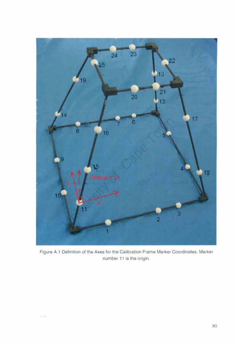
Figure A. 1 Oefin.lIOn oI1he Axes fo r lhe Cal ibratIon Frame Marker Coord inates. Marker
number 11 is the ongln.
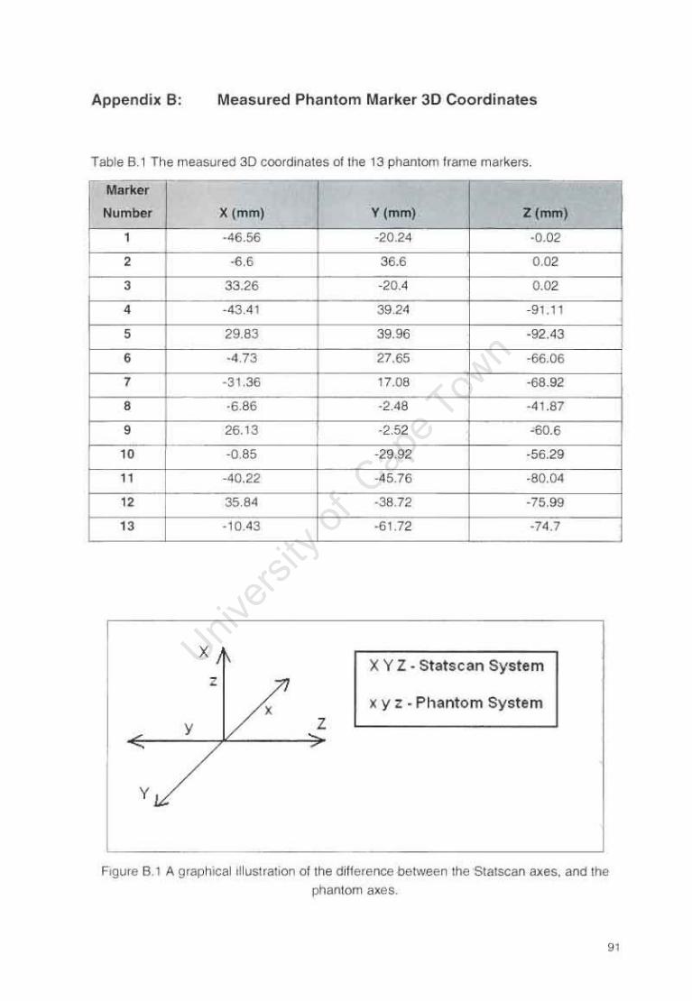
Appendix B: Measured Phantom Marker 30 Coordinates
Table 6, 1 The measured 3D coordinates of the t 3 phantom frame markers.
Markel'"
Number X (mm) Y(mm) Z(mm)
1 -46.56 -20.24 -0.02
2 -6 .6 36.6 0.02
3 33.26 -20.4 0.02
• -43.41 39.24 -91.11
5 29.83 39.96 -92.43 , ·4 ,73 27.65 -66.06
7 -31.36 17.08 -68.92
8 '6,86 ·2.48 -41.87
9 26. 13 ·2.52 '60.6
10 -085 -29.92 -56.29
11 -40.22 -45.76 -80.04
" 35.84 -38.72 -75.99
13 -10.43 -61,72 -74.7
x x y Z - Statscan System
x y z - Phantom System z
Figure B. l A graphlcal li lustrallQrl 01 the difference betweerllhe Slalscan axes. and the
pharltom axes.

Appendix C: MaUab Software Code
This sactJOfI prOVIdes an overview 0/ the Matlab cooe used 10 perform the Image
processing and ma!hemal>Cal translormatlOnS lor the three-dimenslOflal rl3COOStructlOl'lS.
The codes (m·liles) WIN be stored on CD-ROM III the Depa'tment 01 BIomedical
EnglJleenng, UniverSIty 01 Cape Town
Three main codes were used In the e~penmenl$ whICh were then modified to SUit the
speclhc e~penments Suthes wele added to the code names 10 ldenldy Ihe changes.
First. the getmarlls.m coclo IS lhe markel correctlOfl program The output of "getmarks.m"
IS used ,n the "Run m" code. wnlCh calls "calcpolnls.m" 10 perlorm lhe 30 reconSlf\lCtJOfl.
The ne~t code IS "Evaluate.m", which uses the data saved by "Aun m" 10 pioIthe data.
Program to locate the marker centroids - '·getmarks.m"
The input 0/ this program Is Ihe X·ray Image Wllh markers. and The ovtput is an array 01 the
marker x and y coordinates. This code requires user Input 10 select the markers in the
correct sequence.
An X· ray image IS read Into the Matlab workspace and the user IS then prompled 10
klenlily each marker by uSing the mouse and cursor. Each marker IS labelled ae<:ordrng to
the user seteclion. A reglOll of interest is then del ined for each marker uSing lhe user
defined points as a relerence. The program identifies the centroid by using thresholding in
the reglOll 01 ,nterest and the ceT\trOld coord inates are rounded otl 10 the nearest pixel
values.
The "getmarks_phamom,m" code dlflers from "gctmarks.m" by USing a smallor reglOO 01
mterest due to the smaller phanlom markers compared \0 calibrat ion markers The
program also uses a Matlab lunclJOn to identify the centroid,
Program to define the control points and les t points - " Aun.m"
After gatherrng all the necessary 20 marker dala Irom stereo· Images, lhe 20 coordinates
ale then used III the Run,m code ThoS code first defines the known 30 marker coordinateS
and then loads the 20 sterco-image coordinates Dependrng 01'1 the use, lhe IiS1S
(configuralt011S) 01 control pornts and tesl potrlis are defll\ed Mra ThIS program uses a lor·
loop 10 per10fm the 30 fecOflstruchon on the dlfterenl X·ray stereo-pairs The program
"

calls another code, ·caicpomlS,m", which COI1talns the alQOflthms to perlorm the 30
leconstlUCllOn. In tum, "caIcpolms.m" uses proglams called "make_A m" arld
"BACKSU8.m" In Ille calculauon. The ourputs 01 "calcpolnts.m" are the ciflelen:es
between the known 30 coordinates and the calCIJlated 30 coordinates. These values are
saved by "Run,m",
Program to organise and plot the results - " Evaluate.m"
This program loads the data files that were saved by "Run.m" and orgarnses the re$U11S so
that the data can be pIoned as she ........ In Chaptel 4. The program coocatenates the results
Irom like sets 01 data and calculat8s the mean absolute errors. The resultantS and
standard deviatIOns are also perlormed hefe.

Appendix 0 : Experiment Data Tables
Table 01 The Siandarcl deVlal10llS (SO) IOf nne salS of 20 callbra1lOn Irame marl<er
COOfdlnales obtained USIng !he marker COfrecoon program (0' scanning angle.
lmage"sel B).
0 0
o~ 1
Jt ~ ~
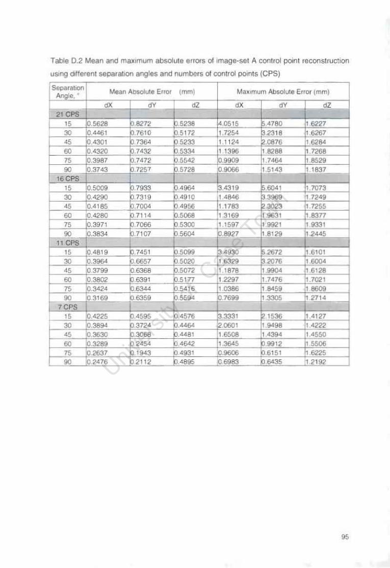
Table 0.2 Mean and ma~lmum absdule errOls oIlmage·sel A conlrol poinlleconslructlon
USing Qtte<enl separatiOll angles and numbers 01 conlrol points (CPS)
Mean Absolule Erf(l' (mm) MaXimum Absolute error (mm)
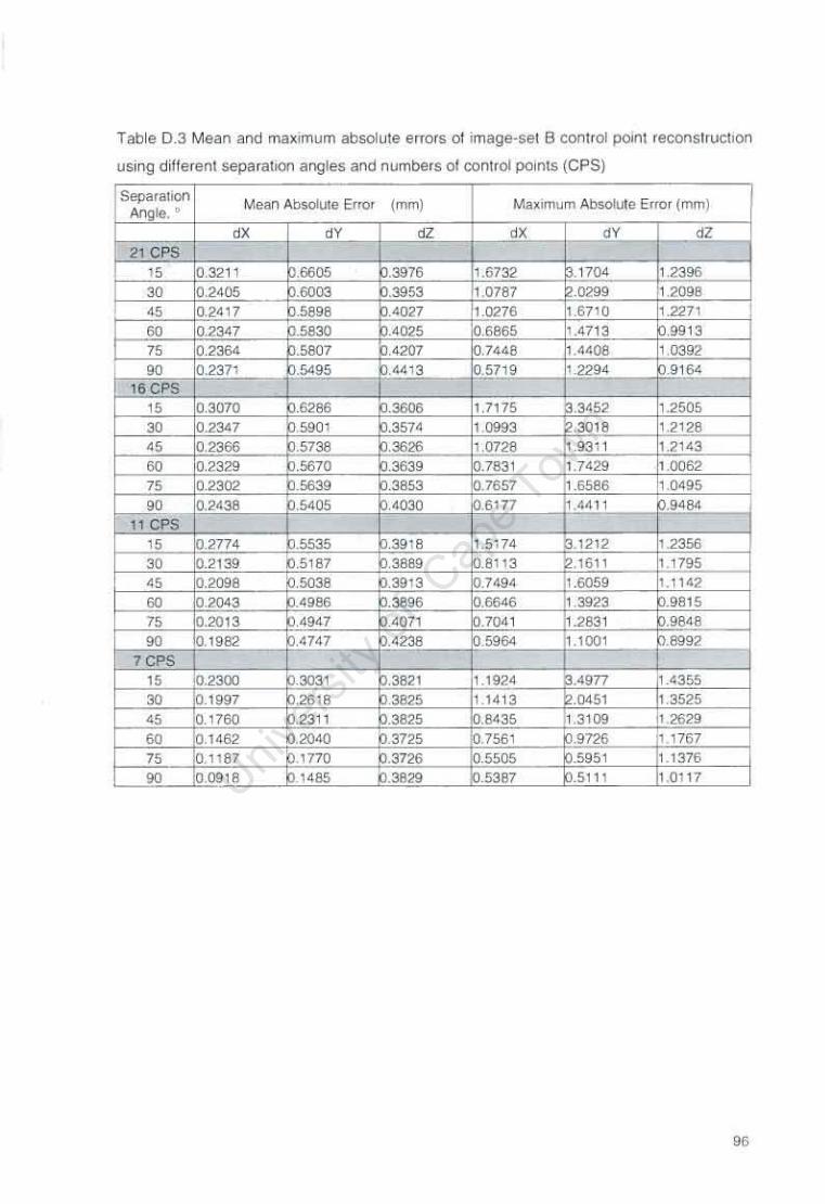
Table 0_3 Mean and maximum absolute errors ot image-set B control potnt reconstruCllOn
using different separat'OI1 aflgles afld numbers of control points (CPS)
Mean AbsolUie Error (mm) Maximum Absolll1e Error (mm)
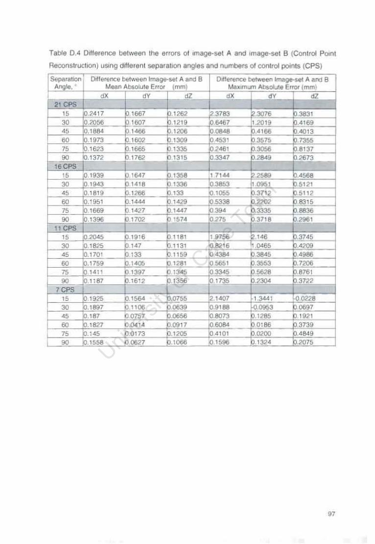
Table 0.4 Orf!erence between the errors at ,mage-set A and 'mage-set B (Control Potnt
ReconstruChOtl) uSing different separal,OO angles arid numbers 01 control points (CPS)
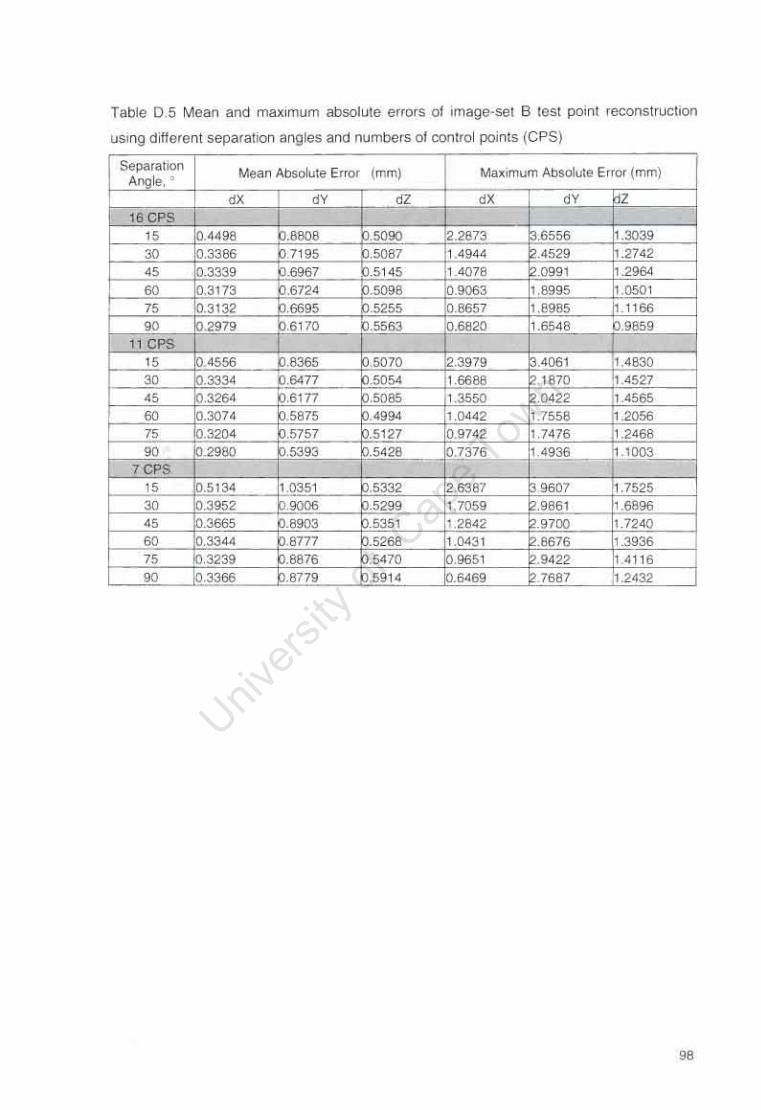
Table 05 Mean and maximum absolule errors of Image-set B lest point re<:onstruCllOn
usmg d ifferent separation angles and numbers of control points (CPS)
Mean Absolute Error (mm) MaXimum Absolute ErrOl (mml
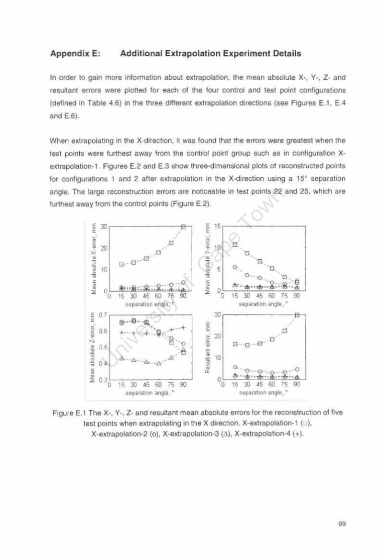
Appendix E: Addit ional Extrapolation Experiment Details
In order 10 gain more informatton about extrapolation. the mean absolute X-, Yo, Z· and
resuhant errors were pIoned 'Of each of the tour control and test point configuratIOns
(detloed In Table 4.6) in the three different extrapolation directJons (see Figures E. ! , EA
and E.6).
When eKtrapole1tng In the X·directlOn. ~ was 10000nd that the errors were greatest when the
test POintS were furthest away Irom the cootrol point group such as in cooiigumllon X·
extrapolation·' Figures E.2 and E.3 show three-dimensional plots 01 reconstl'lJ(;led poln1s
lor contigurations , and 2 alief extrapola tion In Ihe X-directloo using a 15° separation
angle. The large reconstructiorr errors are noticeable In test points 22 and 25, which ere
lunhast away Irom the control points (Figure E.2).
! D ! " , '" ! • D '0 ~
x .0 ." • 0".0 • , .. i n , G ' 0 • " • , • • '0 .. 0. "U
" '",Q",,-. .• ()"o 0 '. . S • • S. " .!h' ..... g,. ;jI: , . '" •
00 •
00 > D ., ., " '" >
" D " .,
" '" " fI~rOl,1)fI "'~t,· "p""oQn angl •. • , " D ,
IJo"O· ·-G. , • 06 '. + .. ~ ,
.0 • + .. + . -+- .1jI< q, - 8"0 , o ."
0 • " • 0
i ~.
~: . e 5 " • 6 ....... tt..- ,
• o. • 0 • 0 • • • > "0 " . , .. " '"
00
" D " eo " '" D '~.,",+On "'~II • II~""!""'~ ..
Figure E. ! The X" Y" z - and resuttant mean absolute erTors tor Ihe reconstruction ot l ive
lest POIn1S when extrapolating ln the X dlr8Cllon, X·exlrepotatIO/'l·' ( ).
X·axtrapo!a!Klo-2 (0), X-extrapolation·3 (L\) , X·exlrapolatlon-4 (+).
..
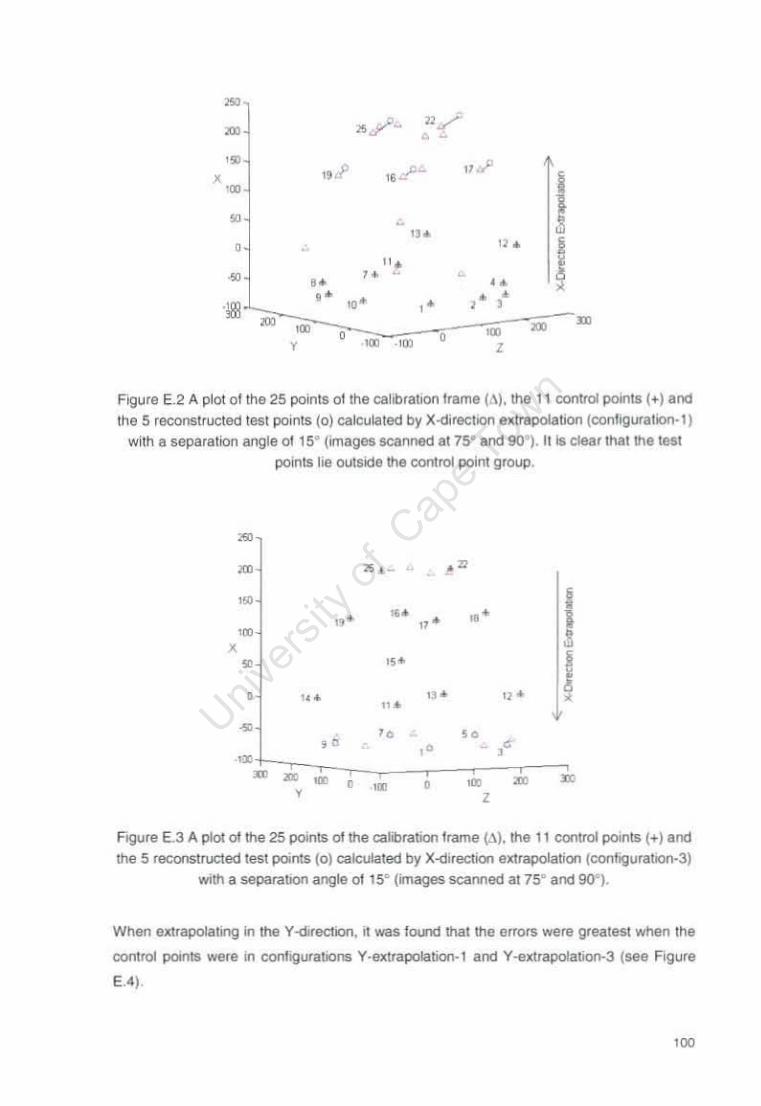
~
m 'J5/-- 2:1./ • '. " ,p ,,-, ~.
I , 18 -. , . • •
'" 0 ", ! '" ~ ,. "
" " " 10" "
• 181 "
, '" m ,.
~ m 0 ,. .,. 0 , ,
FIgure E.2 A plot ot the 25 points altho calibratlOll Irame ("'). the 11 control points (+) and
Ihe 5 r~onstructed lest points (0) calcu~led by X-dirOCIIOO extrapolation (conligura lion- l)
with a separation angle 01 IS' (Images scanned at 75' and 90'), 1116 clear tt!alltle test
points he outside mil 0001/01 po!nt group.
~
m " - ."
'. i ,, ' •• .' ,, ' ,. ~ ,
• I~" I ". ", 0 ... , ". ~
" .. "
, ,. " ,
m m ~ m 0 ,. • ,. , , Figure E.3 A plot 01 the 25 points of the calibra!JOr1 frame (~). the 11 control potnts (+1 and
lhe .5 reconslfucted test pants (0) calculated by X-d'rectKlll extrapolation /coo6gurallOn-3) wilh II separa\JOfl angle of ISO (images scanoed al 75· and go'),
Whllfl extrapolallng in the Y-directlOO. II was fOl,lfld thai the errors were grealesl when the
control points wele in conliguratJ::Ins Y-extrapolalion-l and V-e.trapolahon-3 (see FIgure
E.4) .
'00
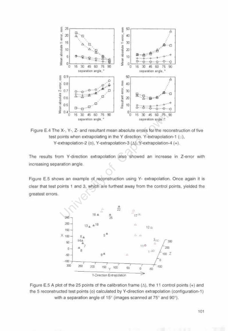
! ~ I~ ~ ' • • ~ • ' " ..
i ~~ .. • " • " ,P 0 • • i " ., ~ 1 ~ .' ." , • , ~" . " " 'l • "
~· ,e ;: I!'· ... + ..• . -..... ... .. + . , . . ~ :: :~ , 1)."0" " 0 ··-0"9 i " J " " ~ ~ .. n .. " ~ ~ .. "
.., ..,_ ........ ..~ .... .", &0,0. '
I" ..,
0 0 l (18 ,0 • 1 " .. ~.
I .. 01 0- _0··4) -0,_ D ~ .A . CJ • 1: :1; ~ .<I& ,. .. ~ 1" 0 • " ". .: •. ·0 '
'" 0 1 " .. " , rJ. .iJ '-C· • 6:-·t··;:· · ... ·· .... f 0 .
0
. ··o-·.()·-o
" ~ 6 .. " .., " " ~ ., .. , .., . .,- ...... ..,..r .. ""' ......
FIQure E.4 The X" '(-, Z· and resultant mean absolute errors fOf the reconstruction 01 five lest points when eXlrapolatng in the Y direcbon. Y-extrapolation-' ( ).
Y-extrapol,ltIon-2 (0). Y-el(Uapo!ation-3 CAl, Y·extrllpolation-4 (+).
The fesults 110m Y·dlrectlOf1 eX1rapolabon also showed an Increase in Z-error with
Increasing separation angle
Figure E.S snows an example of reconsuUCTIOfl USing y. exrrapolation. Once again it is
Clear that test points 1 and 3. WhICh are furthest away 1,0m the control points, yielded the
greatest errors.
, " ", ,
~ ~
m 13 .... 18 ,,., X,.
" " • .. , , , , , ,
~ " .~
m ~ ~ ,ro • ,. ,., V-001'ttJon~~
Figure E.5 A plot 01 the 25 points ot the calibratIon !rame (n), the 11 control POInts (+) and
ltIe 5 recorlStructed test points (0) calculated by Y-directjoo extrapoiahOfl (conl lguration· ' )
WIth a separa tion angle 01 IS' (Images scanned at 15' and 90' ).
'"

As with the e~trapolation in ttle X and Y directIOnS. the Z·dirflCtlon e~trapola tion accuracy
is shown \Q clepend on the control and test point configuration (see Figure E.6). For the
mafOrit)l 01 configurations chosen, the x and Y mean absolute erfO/"S decrease with
increasll1g separation engle and this ca'1 be anribulitd to there being more InformatIOn
available for the gen81'ation 01 these coordinates when the separation angie is lalge
Figure E.7 shows an e~ample ot raconstvctlOn USIng Z· extrapolation. The reC01'1structlon
Is much mo.'e accurate than thaI 01 X and Y direction e)(lrapolallon and Is similar to
reconstruction without extrapolation.
, "' ! " ~.
! " I D "- " • • • " i). .1·::~ .. +-·.t:.'- • • • " & Q' .• ' 1:; ' -> • " •• "" . • 01). •.• "" •• & i .;; :':e:' .-.1>', 01). 0 • • ·0 .-(t • • " D. • " •
• 0··0··[1 .. -0 D • 0 • • 010
• , " ~ ~ "' " •
, '0 " ~ ~ " " ~ ~'","'II,.n an~I.<· .. p~'~nOtl."gl •• , " .c .. a , ,
~. [1"0··[1'·
" D , " ~ ~ • I 06 [3-··0··0 o ··-E]' " $: .. iF' "" .. a."iiI" 4
, li. • • .• , .... ;;g,'~ . 6 • " • " • • ... +. + . • .. -+- • • i "0 "0 " " ~ '" " ~ " " ~ "' "
., "pal"oon onvIe<' np .. O! .. n "ng/t •
Figure E,6 The X·. Y •. Z· and resultant !Tean absolute elT()f1; for the recoostruclloll or Ijye test pomts when e)(l rapolating I'l the Z dtrecron. Z·extrapolatlon· t (l.
Z·elClrapoiallOn·2 (0), Z·extlfPOlation-3 (t.). Z·eJdrapoiatlOn·4 (.1.
'"
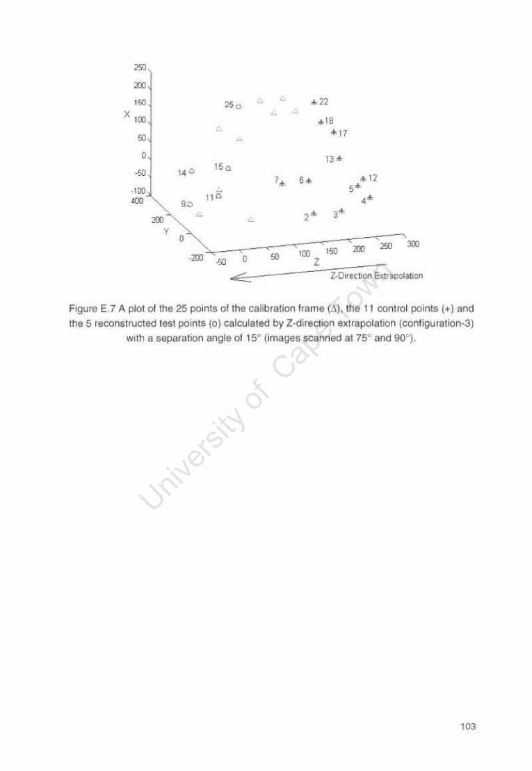
'" ;m
,~ "0 ."
X '00 ... c ." ~
• ". .~ ,, 0 "0
'. 6. ,j, 12
· '00 " ... ,,0 "
" " ,.,
'" '" '00 ". '" ." 0 " Z
...-:- Z-OnclJOn &:trapolilllOn
Figure E.7 A plot of the 25 points 01 the calibration frame (aj. the 11 control points (T) and lhe 5 reconslruc1ed lest points (0) calculated by Z-direction Q)(lrapolauon (configuraHon-3)
with a separation angle ol lSD Omages scanned al 75° aocl 90").
""
References
Abdel-A1-lz VI. Karara HM (1971) Oi reel Lmear Iranslormallon Irom comparalor
coordmale! 11110 obioct-space coordinates In Proc ASP/UI Symposl(Jm on Clos(} Rango
Phologrammelry. AmeliCan Society 01 Pt1ologrammetry. Fal ls Church pp I - 18
Adams LP (1981) X-ra~ stereo phologrammelry locating the precise. lhree dimensIOnal
position 01 Image pamls, MedIcal & BlOk>glCal EnglflOOnng & Computing, 19: 569 - 578.
Adams LP. Constanl OA (1988) Boosleuometncs In the study 01 !he morpllology 01 !he
lumbar sacral SPIne Mcdtcal & &%gIcaI Engrneenng & Computiflg 26, 383 - 388.
Alberll.lS P. Malmberg M PefSSOn S. Selllik G (1990) Vanablhly 01 measurements 01 cranial growlh In !he rabbit Amencan Journal 01 Ana/omy. 188. 393 - 400
Allaro·Adrlan J. Gill HS Muflay OW (1999) Cement migratIOn OI lier THR A companson 01
Charnley Ellie and b eler Femoral SIems usmg ASA The Journal 01 Bone arld Joml
S(Jrgory.8 ' 130- 134
AndrE! S, Dansereau J. Labelle H (1994) Ophm,zed verllCal slereo base radIOgraph(; selup
lor the c liniCal ,hree-dlmenslonal reconSlrUCllOn 01 Ihe human spone Journal of BIOmechanics, 27 (8) . 1023 - 1035.
Aronson 5, Jonsson N. Atberius P (1985) Tantatum markers In rad'09raphy An
assessmen' ollissue reac,.ons. Skeletal Radiology, 14 (31' 207 - 21 1
Aubin C-L Oafl$t!r-ellu J. Parenl r , Llibelle II, ckI QUIse JA (1997) MorphometrIC
evalu.allOns 01 personalised 3D reconstructIOns andgeomelrlC models 01 the human spme
MedICal & BIologICal Engmeenng & Computmg, 35: 61 I - 61 8
Baumnnd S. Mol'" FH. CUlly 5 (1983) The g&emelfy or 'hree dimenSional measurement
hom coplanar It-ray .mages Amencan Journal 01 OffhodonflCS. 84; 313 - 322
Benameur S. MIgnone M. Parent 5 , Labelle H Skill" W de GuISe J (2003) 3D f 20
reglsuahon and segmentatIOn 01 scoIlobc vertebrae lIsong stahStlC8l models. Compu/eflzecj
Mool(;ai lmagmg and Graphics 27 321 . 327
Bennrngfield SJ. Potg18ter H NICOl A. vall As 5 , Bowl!! G. Henng G. Lat\l E (2003) Report
OIl a new type or trauma Iltll-bOOy d,g'lal X·ray machine Emerging Rad/okJgy. 10. 23 - 29.
''''
Berg DC, Hill DL, Raso VJ, Lou E, Church T, Moreau MJ, Mahood JK (2002) Using threedimensional difference maps to assess -changes in scoliotic deformities. Medica} &
Biological Engineering & Computing, 40: 290 - 295.
Bice WS, Dubois OF, Prete JJ, Prestidge SR (1999) Source localisation from axial image sets by iterative relaxation of the nearest neighbour criterion. Medical Physics, 26: 1919-1924.
Berlin N (1997) High precision measurements in digital radiographs. UmeA University, Sweden.
Berlin N, Thien T, Karrholm J (2002) The precision of radiostereometric measurements. Manual vs. digital measurements. Journal of Biomechanics, 35: 69 - 79.
Bragdon CR, Estok OM, Malchau H, Karrholm J, Yuan X, Bourne R, Veldhoven J, Harris WH (2003) Comparison of two digital radiostereometric analysis methods in the determination of femoral head penetration In a total hip replacement phantom. Journal of Orthopaedic Research, 22 (3): 659 - 664.
Broadbent BH (1931) A new x-ray technique and its application to orthodontia. Angle Orthodontist, pp. 1-45.
Cai J, Chu JCH, Saxena VA, Lanzi LH (1997) A method for more efficient source localization of interstitial implants with biplane radiographs. Medical Physics, 24: 1229-1234.
ChalliS JH, Kerwin DG (1992) Accuracy assessment and control point configuration when using DLT for photogrammetry. Journal of Biomechanics, 25: 1053 - 1058.
Chen L, Armstrong CW, Raftopoulos DO (1994) An investigation on the accuracy of the direct linear transformation technique. Journal of Biomechanics, 27: 493 - 500.
Choo AMT, Oxland TR (2003) Improved RSA accuracy with DL T and balanced calibration marker distributions with an assessment of initial calibration. Journal of Biomechanics, 36: 259-264.
Dansereau J, Stokes IA (1988) Measurements of the three-dimensional shape of the rib cage. Journal of Biomechanics, 21 (11): 893 -901.
De Lange A, Huiskes R, Kauer JMG (1990) Measurement errors in RoentgenStereophotogramrnetric Joint Motion Analysis. Journal of Biomechanics, 23 (3): 259 -269.
105
Djerf K, Edholm P, Hedbrant J (1987) A simplified Roentgen Stereo-photogrammetric Method: Analysis of small movements between the prosthetic stem and the femur after total hip replacement. Acta Radiologiea, 28: 603 - 606.
Douglas TS, Meintjes EM, Vaughan Cl, Viljoen D (2003) The role of depth in eye distance measurements: comparison of single and stereophotogrammetry. American Journal of Human Biology, 14: 573 - 578.
Douglas TS, Vaughan Cl, Wynne SM (2004) Three-dimensional point localisation in Iowdose X-ray images using stereophotogrammetry. Medical & Biological Engineering &
Computing, 42: 37 - 43.
Gall K, Verhey l (1993) Computer-assisted positioning of radiotherapy patients using implanted radio-opaque fiducials. Medical Physics, 20 (4): 1153 -1159.
Gazzani F (1993) Comparative assessment of two algorithms for calibrating stereophotogrammetric systems. Journal of Biomechanics, 26 (12): 1449 - 1454.
Gussekloo SWS, Janssen BAM, Vosselan MG, Bout RG (2000) A single camera roentgen stereophotogrammetry method for static displacement analysis. Journal of Biomechanics, 33: 759-763.
Hallert B (1960) Photogrammetry: Basic Principles and General Survey. McGraw-Hil1800k Company Inc, New York.
Hatze H (1988) High preCision 3D photogrammetric calibration and object space reconstruction using a modified DlT-approach. Journal of Biomechanics, 21(7): 533-538.
Hinrichs RN, Mclean SP (1995) Nl T and extrapolated Dl T: 3D cinematography alternatives for enlarging the volume of calibration. Journal of Biomechanics, 28 (10): 1219 -1223.
Jackson DD (1983) An automatic method for localizing radioactive seeds in implant dosimetry. Medical Physics 10 (3): 370 - 372.
Johnsson R, Axelsson P, Gunnarsson G, Stromqvist B (1999) Stability of lumbar Fusion with Transpedicular Fixation determined by Roentgen Stereophotogrammetric Analysis. Spine, 24 (7): 687 - 690.
Judge AW (1926) Stereoscopic Photography: Its application to science, industry and education. Chapman & Hall Ltd. london, pp. 200 - 209.
106

Kalmar JA, Jones JP, Merritt CRB (1994) low-dose radiography of scoliosis in children: A comparison of methods. Spine, 19: 818 - 823.
Kaptein Bl, Valstar ER, Spoor CW, Soel Be, Rozing PM {20(6) Model-based RSA of a femoral hip stem using surface and geometrical shape models. Clinical Orthopaedics & Related Research. 488: 92 - 97.
Kaptein Bl, Valstar ER, Stoel BC, Rozing PM, Retber JH (2003) A new model-based RSA method validating using CAD models and models from r:eversed engineering. Joumal of Biomechanics. 36: 873 - 882.
Kaptein Bl, Valstar ER, Stoel BC, Rozing PM, Reiber JH (2005) A new type of modelbased Roentgen stereophotogrammetric analysis for solving the occluded marker problem. Joumal of Biomechanics. 38: 2330 - 2334.
Karrholm J, Elmqvist lG, Selvik G, Hansson LI (1989) Chronic Anterolateral instability of
the knee - A roentgen stereophotogrammetric evaluation. The American Joumal.of Sports Medicine, 17 (4): 555 - 563.
Kiss J, Murray OW, Turner-smith AR, Bithell J, Bulstrode CJ (1996) Migration of cemented femoral components after THR. The Joumal of Bone & Joint Surgery, pp 796 - 801.
KofmanJ, Miller 01, Knopf GK, Zecevic A (1998) Calibration and measurement' accuracy of a stereophotogrammetric system using the Oir.ect Linear Transformation. North American Congress on Biomechanics, http://asb-biomech.org/NACOB98/107
Kreel, l (1981) Clark's Positioning in Radiography, Tenth Edition, Vol. 2. William Heinemann Medical Books Ltd, London. pp 704 - 707.
Kusnoto B, Evans CA, Begole EA, de Rijk W (1999) Assessment of 3-dimensional computer generated cephalometric measurements. American Joumal of Orthodontics and DentofacialOrthopedics, 166: 390 - 399.
Kwon V-H, http://kwon3d.comltheorv/dltldlt.htrnl, 8all State University, Biomechanics Laboratory, United States of America. last accessed January 2006.
lam Kl, Ten Haken RK (1991) Improvement of precision in spatial localisation of radioopaque markers using the two-film technique. Medical Physics, 18 ~6): 1126 - 1131.
lam Kl, Ten Haken RK, McShan Ol, Thornton AF (1993) Automated determination of patient set-up errors in radiation therapy using spherical radio-opaque markers. Medical Physics, 20 (4): 1145 -1152.
107
Li S, Chen GTY, Pelizzari CA, Reft C, Roeske JC, lu Y (1996) A new source localization algorithm with no requirement of one-to-one source correspondence between biplane
radiographs. Medical Physics, 23: 921 - 927.
Martel MK, Narayana V (1998) Brachytherapy for the Next Century: Use of Image Based
Treatment Planning. Radiation Research, 150: S178 - S188.
Marzan GT, Karara HM (1975) A computer program for direct linear transformation solution of the collinearity condition, and some applications of it. Symposium on Close
Range Photogrammetric Systems. American Society of Photogrammetry. Falls Church,
pp. 420 - 476.
Medcyclopaedia, Last accessed October 2006. http://www.medcyclopaedia.comllibrarv/topics/volume its/scanoq ram .aspx
Meintjes EM, Douglas TS, Martinez F, Vaughan Cl, Adams lP, Stekhoven A, Viljoen D (2002) A stereophotogrammetric method to measure the facial dysmorphology of children in the diagnosis of Fetal Alcohol Syndrome. Medical Engineering Physics, 24: 683 - 689.
Mitchell Hl, Newton I (2002) Medical photogrammetric measurement: overview and prospects. ISPRS Journal of Photogrammetry & Remote Sensing, 56: 286 - 294.
Mitton D, landry C, Veron S, Skalli W, Lavaste F, De Guise J.A (2000) 3D reconstruction method from biplanar radiography using non-stereocorresponding pOints and elastic deformable meshes. Medical & Biological Engineering & Computing, 38: 133-139.
Mitulescu A, Semaan I, De Guise JA, leborgne P, Adamsbaum C, Skalli A (2001)
Validation of the non-stereo corresponding points stereoradiographic 3D reconstruction technique. Medical & Biological Engineering & Computing, 39: 152-158.
Moffit FH (1967) Photogrammetry, International Textbook Company, Pennsylvania, pp. 174 -177.
Morin Doody M, Lonstein JE, Stovall M, Hacker DG, luckyanov N, Land CE (2000) Breast cancer mortality after diagnostic radiography: Findings from the U.S. Scoliosis Cohort Study. Spine, 25 (16): 2052-2063.
Nelissen RGHH, Valstar ER, Rozing PM (1998) The effect of hydroxyapatite on the micromotion of total knee prostheses: A randomised, double-blind study. Journal of Bone
and Joint Surgery [Am]. SO-A (11): 1665 - 1672.
108
Nilsson KG, Karrholm J (1996) RSA in the assessment of aseptic loosening. The Joumal of Bone & Joint Surgery, 78B (1): 1 - 3.
Nystrom L, Soderkvist I, Wedin P (1994) Technical Note: A note on $)ffle identification
problems arising in Roentgen Ster:eophotogrammetric Analysis. Joumal of Biomechanics, 27 (10): 1291 - 1294.
Cnsten I, Akesson K, Besjakov J, Obrant KJ (1995) Migration of the Charnley stem in
Rheumatoid arthritis & osteoarthritis. The Journal of Bone & Joint Surgery, pp. 18 - 22.
Ostgaard SE, Gottlieb L, Toksvig-Larson S, Lebech A. Talbot A & Lund B (1997) Technical
Note: Roentgen Stereophotogrammetric Analysis using computer-based image-anatysis.
Joumal of Biomechanics, 30 (9): 993 - 995.
Papadopoulos MA, Christou PK, Athanasiou AE, Boettcher P, Zeilhofer HF, Sader R,
Papadopoulos NA (2002) Three dimensional craniofacial recoRstruction imaging. Oral
Surgery, Oral Medicine, Oral Pathology, Oral Radiol. Endod., 93: 382 - 393.
Petit Y, Dansereau J, Labelle H, de Guise JA (1998) Estimation of 3D location and
orientation of human vertebral facet joints from standing digital radiographs. Medical & Biological Engineering & Computing, 36: 389 - 394.
Plamondon A. Gagonon M (1991) Effect of the configuration of data acquisition on the
accuracy of a stereoradiographic system. Medical & Biological Engineering & Computing, 29: 620 - 622.
Ras F, Habets LLMH, van Ginkel FC, Prahl-Andersen B (1996) Quantification of facial
morphology using stereophotogrammetry - demonstration of a new concept. Joumal of Dentistry. 24: 369 - 374.
Rogus RD, Stern RL, Kubo HD (1999) Accuracy of a photogrammetry-based patient
positioning and monitoring system for radiation therapy. Medical Physics, 26 (5): 721 -
728.
RSA Biomedical website, http://www.rsabiomedical.se. Last accessed Sep~mber 2006.
Ryd L, Albrektsson BEJ, Herberts P, Lindstrand A, Selvik G (1986) Micromotion of non
cemented Freeman-Samuelson knee prostheses in Gonarthrosis. Clinical Orthopaedics & Related Research. pp: 205-212.
Ryd L, Yuan X, Lofgren H (2000) Methods for determining the accuracy of
radiostereometric analysis (RSA). Acta Orthopaedica Scandinavia, 71 {4): 403-8.
109
Selvik G (1989) Roentgen Stereophotogrammetry, A method for the study of the
kinematics of the skeletal system. Acta Orthopaedica Scandinavia Supplement, 232: 1-51
Selvik G, Alberius P & Aronson AS (1983) A Roentgen Stereophotogrammetric System.
Construction, calibration and technical accuracy. Acta Radiologica Diagnosis, 24: 343-352.
Siddon RL, Chin LM (1985) Two-film Brachytherapy reconstruction algOrithm. Medical
Physics, 12: 77-83.
Slama CC, Theurer C, Henriksen SW (1980) Manual of Photogramrnetry, Fourth Edition, American Society of Photogrammetry, pp. 846-857.
Stefansic JD, Herline AJ, Shyr Y, Chapman WC, Fitzmatrick JM, Dawant BM,
Galloway RL (2000) Registration of Physical Space to Laparoscopic Image Space for Use
in Minimally Invasive Hepatic Surgery. IEEE Transactions on Medical Imaging, 19 (10): 1012-1023.
Valstar ER, Botha CP, van der Glas M, Rozing PM, van der Helm FCT, Post FH,
Vossepoel AM (2002) Towards computer-assisted surgery in shoulder joint replacement.
ISPRS Journal of Photogrammetry and Remote Sensing, 56: 326 - 337.
Valstar ER, de Jong FW, Vrooman HA, Rozing PM, Reiber JHC (2001) Model based Roentgen Stereophotogrammetry of orthopaedic implants. Journal of Biomechanics, 34:
715-722.
Valstar ER, Gill R, Ryd L, Flivik G, Borlin N, Karholm J (2005) Guidelines for standardization of radiostereometery (RSA) of implants. Acta Orthopaedica, 76: 563 -
572.
Valstar ER, Nelissen RGHH, Reiber JHC, Rozing PM (2002) The use of Roentgen
Stereophotogrammetry to study micromotion of orthopaedic implants. ISPRS Journal of
Photogrammetry and Remote Sensing, 56: 376 - 389.
Van der Vlugt G (1991) The development of a real-time photogrammetric system for
patient positioning in proton therapy. Dissertation, University of Cape Town.
Van Geems BA (1996) The use of multiple surviews of a computed tomography scanner to determine the 3D coordinates of external cranial markers. International Archive of
Photogrammetry and Remote SenSing, 31: 576 - 580.
Van Geems BA (1997) The Development of a simple stereotatic device for neurosurgical
applications. Dissertation, University of Cape Town, pp: 34 - 47; 192 - 199.
110
Van Geems BA, Adams LP, Hough J (1995) The use of a two .dimensional projective
transform to solve for the parameters for the anterior-posterior and ~ateral surviews of aCT scan. Intemational Archive of Photogrammetry and Remote Sensing, 30, pp. 366 - 371.
Veress SA (1989) X-Ray Photogrammetry, Systems, and Applications. Non-Topographic Photogrammetry, Editor: Karara HM. American Society for Photogrammetry and Remote Sensing, Second Edition, pp. 167 - 186.
Vrooman HA, Valstar ER, Brand GJ, Admiraai DR, Rozing PM, Reiber JHC (1998) Fast and accurate automatic measurements in digitized stereophotogrammetric radiographs.
Journal of Biomechanics, 31: 491 - 498.
Wang S, Jones NB, Richardson JB, Klaassens E (1996) Optimtsed method for locating reference markers in Roentgen stereophotogrammetric analysis of orthopaedic radiographs. Medical & Biological Engineering & Computing, 34: 88 - 92.
Weisz I, Jefferson RJ, Carr AJ, Tumer-Smith AR, Mclnemey A, Houghton GR (1989) Back
shape in brace treatment of idiopathic scoliosis. Clinical Orthopaedics and Related Research, 240: 157 - 163.
Wood GA, Marshall RN (1986) The accuracy of DLT extrapolation in three-dimensional film analysis. Joumal of Biomechanics, 19: 781 -785.
Yuan X, Ryd L (2000) Technical Note: Accuracy analysis for RSA: a computer simulation study on 3D marker reconstruction. Journal of Biomechanics, 33: 493 - 498.
ZIII DG, Cullen MR (1992) Advanced Engineering Mathematics. PWS publishing company, Boston, pp. 465 - 468.
111