Local Search Algorithms

Local Search

Combinatorial problems...

• involve finding a grouping, ordering, or assignment of a discrete set of objects which satisfies certain constraints

• arise in many domains of computer science and various application areas

• have high computational complexity (NP-hard)

• are solved in practice by searching an exponentially large space of candidate / partial solutions

Examples for combinatorial problems:

• finding shortest/cheapest round trips (TSP)

• finding models of propositional formulae (SAT)

• planning, scheduling, time-tabling

• resource allocation

• protein structure prediction

• genome sequence assembly

The Propositional Satisfiability Problem (SAT)

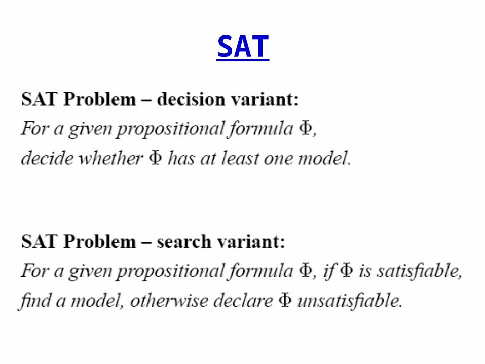
SAT

The Traveling Salesperson Problem (TSP)

• TSP – optimization variant:• For a given weighted graph G = (V,E,w),

find a Hamiltonian cycle in G with minimal weight,

• i.e., find the shortest round-trip visiting each vertex exactly once.

• TSP – decision variant:• For a given weighted graph G = (V,E,w),

decide whether a Hamiltonian cycle with minimal weight ≤ b exists in G.

TSP instance: shortest round trip through 532 US cities

Search Methods

• Types of search methods:

• systematic ←→ local search

• deterministic ←→ stochastic

• sequential ←→ parallel

Local Search (LS) Algorithms

• search space S

(SAT: set of all complete truth assignments to propositional variables)

• solution set

(SAT: models of given formula)• neighborhood relation

(SAT: neighboring variable assignments differ in the

truth value of exactly one variable)• evaluation function g : S → R+

(SAT: number of clauses unsatisfied under given

assignment)

SS '

SxSN

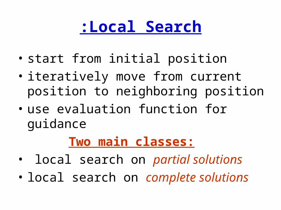
Local Search:

• start from initial position

• iteratively move from current position to neighboring position

• use evaluation function for guidance

Two main classes:

• local search on partial solutions

• local search on complete solutions

local search on partial solutions

• Order the variables in some order.

• Span a tree such that at each level a given value is assigned a value.

• Perform a depth-first search.

• But, use heuristics to guide the search. Choose the best child according to some heuristics. (DFS with node ordering)

Local search for partial solutions

Construction Heuristics for partial solutions

• search space: space of partial solutions

• search steps: extend partial solutions with assignment for the next element

• solution elements are often ranked according to a greedy evaluation function

Nearest Neighbor heuristic for the TSP:

Nearest neighbor tour through 532 US cities

DFS

• Once a solution has been found (with the first dive into the tree) we can continue search the tree with DFS and backtracking.

• In fact, this is what we did with DFBnB.

• DFBnB with node ordering.

Limited Discrepancy Search

• At each node, the heuristic prefers one of the children.

• A discrepancy is when you go against the heuristic.

• Perform DFS from the root node with k discrepancies

• Start with k=0• Then increasing k by 1• Stop at anytime.

Number of Discrepancies

011 11 2 2 2 3

• Assume a binary tree where the heuristic always prefers the left child.

Limited Discrepancy Search

Advantages:

• Anytime algorithm

• Solutions are ordered according to heuristics

local search on complete solutions

Iterative Improvement (Greedy Search):

• initialize search at some point of search space

• in each step, move from the current search position to a neighboring position with better evaluation function value

Iterative Improvement for SAT

• initialization: randomly chosen, complete truth assignment

• neighborhood: variable assignments are neighbors iff they differ in truth value of one variable

• neighborhood size: O(n) where n = number of variables

• evaluation function: number of clauses unsatisfied under given assignment

Hill climbing

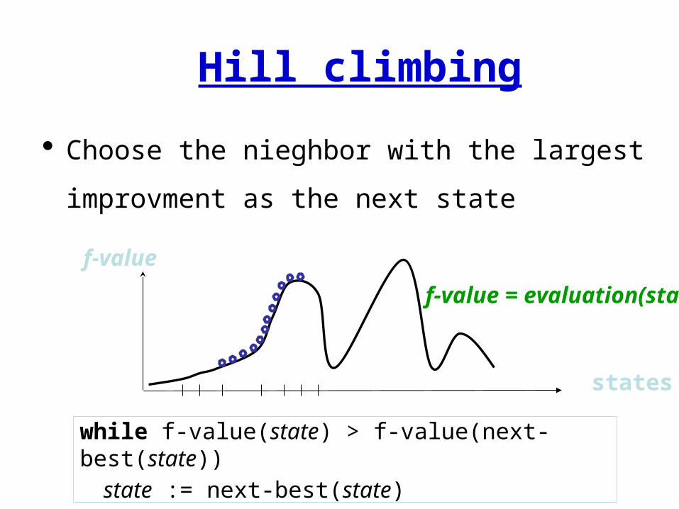
Choose the nieghbor with the largest

improvment as the next state

states

f-value

f-value = evaluation(state)

while f-value(state) > f-value(next-best(state))

state := next-best(state)

Hill climbing

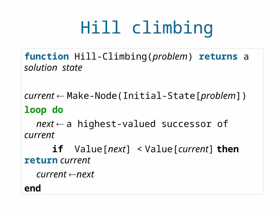
function Hill-Climbing(problem) returns a solution state

current Make-Node(Initial-State[problem])

loop do

next a highest-valued successor of current

if Value[next] < Value[current] then return current

current next

end

Problems with local searchTypical problems with local search (with

hill climbing in particular)

• getting stuck in local optima

• being misguided by evaluation/objective function

Stochastic Local Search

• randomize initialization step

• randomize search steps such that suboptimal/worsening steps are allowed

• improved performance & robustness

• typically, degree of randomization controlled by noise parameter

Stochastic Local Search

Pros:• for many combinatorial problems more efficient

than systematic search• easy to implement• easy to parallelizeCons:• often incomplete (no guarantees for finding

existing solutions)• highly stochastic behavior• often difficult to analyze theoretically/empirically

Simple SLS methods

• Random Search (Blind Guessing):

• In each step, randomly select one element of the search space.

• (Uninformed) RandomWalk:

• In each step, randomly select one of the neighbouring positions of the search space and move there.

Random restart hill climbinghill climbing עלול להיתקע בנקודה שבה אין

התקדמות. נוכל לשפר אותו בצורה הבאה:. hill climbingבחר בנקודה רנדומלית והרץ את 1.אם הפתרון שמצאת טוב יותר מהפתרון הטוב 2.

ביותר שנמצא עד כה – שמור אותו..1חזור ל-3.

מתי נסיים? – לאחר מספר קבוע של איטרציות. – לאחר מספר קבוע של איטרציות שבהן לא נמצא שיפור לפתרון הטוב ביותר

שנמצא עד כה.

Random restart hill climbing

states

f-value

f-value = evaluation(state)

Randomized Iterative Improvement:

• initialize search at some point of search space search steps:

• with probability p, move from current search position to a randomly selected neighboring position

• otherwise, move from current search position to neighboring position with better evaluation function value.

• Has many variations of how to choose the randomly neighbor, and how many of them

• Example: Take 100 steps in one direction (Army mistake correction) – to escape from local optima.

Simulated annealing

Combinatorial search technique inspired by the physical process of annealing [Kirkpatrick et al. 1983, Cerny 1985]

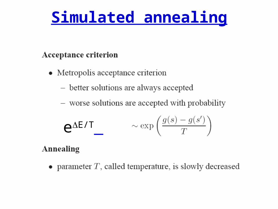
Outline Select a neighbor at random.

If better than current state go there.

Otherwise, go there with some probability.

Probability goes down with time (similar to

temperature cooling)

Simulated annealing

eE/T

Generic choices for annealing schedule

Pseudo codefunction Simulated-Annealing(problem, schedule) returns

solution state

current Make-Node(Initial-State[problem])

for t 1 to infinity

T schedule[t] // T goes downwards.

if T = 0 then return current

next Random-Successor(current)

E f-Value[next] - f-Value[current]

if E > 0 then current next

else current next with probability eE/T

end

Example application to the TSP [Johnson & McGeoch 1997]

baseline implementation:• start with random initial solution• use 2-exchange neighborhood• simple annealing schedule; relatively poor performance improvements:• look-up table for acceptance probabilities• neighborhood pruning• low-temperature starts

Summary-Simulated Annealing

Simulated Annealing . . .

• is historically important

• is easy to implement

• has interesting theoretical properties (convergence), but these are of very limited practical relevance

• achieves good performance often at the cost of substantial run-times

Tabu Search

• Combinatorial search technique which heavily relies on the use of an explicit memory of the search process [Glover 1989, 1990] to guide search process

• memory typically contains only specific attributes of previously seen solutions

• simple tabu search strategies exploit only short term memory

• more complex tabu search strategies exploit long term memory

Tabu search – exploiting short term memory

• in each step, move to best neighboring solution although it may be worse than current one

• to avoid cycles, tabu search tries to avoid revisiting previously seen solutions by basing the memory on attributes of recently seen solutions

• tabu list stores attributes of the tl most recently visited

• solutions; parameter tl is called tabu list length or tabu tenure

• solutions which contain tabu attributes are forbidden

Tabu Search

Problem: previously unseen solutions may be tabu use of aspiration criteria to override tabu status

Stopping criteria:• all neighboring solutions are tabu• maximum number of iterations exceeded• number of iterations without improvement

Robust Tabu Search [Taillard 1991], Reactive Tabu Search[Battiti & Tecchiolli 1994–1997]

Example: Tabu Search for SAT / MAX-SAT

• Neighborhood: assignments which differ in exactly one variable instantiation

• Tabu attributes: variables• Tabu criterion: flipping a variable is

forbidden for a given number of iterations• Aspiration criterion: if flipping a tabu

variable leads to a better solution, the variable’s tabu status is overridden

[Hansen & Jaumard 1990; Selman & Kautz 1994]

Genetic algorithms

• Combinatorial search technique inspired by the evolution of biological species.

• population of individual solutions represented as strings

• individuals within population are evaluated based on their “fitness” (evaluation function value)

• population is manipulated via evolutionary operators

– mutation– crossover– selection

Genetic algorithms

• How to generate the next generation.

• 1) Selection: we select a number of states from the current generation. (we can use the fitness function in any reasonable way)

• 2) crossover : select 2 states and reproduce a child.

• 3) mutation: change some of the genues.

General Genetic algorithm• Pop= initial population• Repeat{• NEW_POP = EMPTY;• for i=1 to POP_SIZE{• x=fit_individual; // natural selection• y=fit_individual;• child=cross_over(x,y);• if(small random probability) • mutate(child);• add child to NEW_POP• }• POP=NEW_POP• } UNTIL solution found• Return(best state in POP)

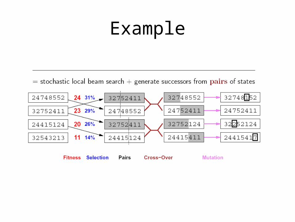
Example

8-queen example

Summary: Genetic Algorithms

Genetic Algorithms• use populations, which leads to increased

search space exploration• allow for a large number of different

implementation choices• typically reach best performance when

using operators that are based on problem characteristics

• achieve good performance on a wide range of problems