Embed Size (px)
Citation preview

Local Reverse Time Migration with Extrapolated VSP Green’s
Function
Xiang Xiao
UTAM, Univ. of Utah
Feb. 7, 2008

2
Outline
Motivation Theory Numerical Tests
Sigsbee VSP data set GOM VSP data set
Conclusions
Motivation Theory Numerical Tests Conclusion

3
VSP Forward Modeling
s
x
g
Motivation
D(g|s)
VSP data
Theory Numerical Tests Conclusion

4
Reverse Time Migration
s
x
g
Motivation
D(g|s)
VSP data
Theory Numerical Tests Conclusion

5
Reverse Time Migration
s
x
G(x|g) g
G(x|s)
BackwardD(g|s)
Forwardsource
m(x) ~ s
~ ds G(x|s)
Forward source
G(x|g)* D(g|s)dg
Backward data
g
*
Motivation Theory Numerical Tests Conclusion
6
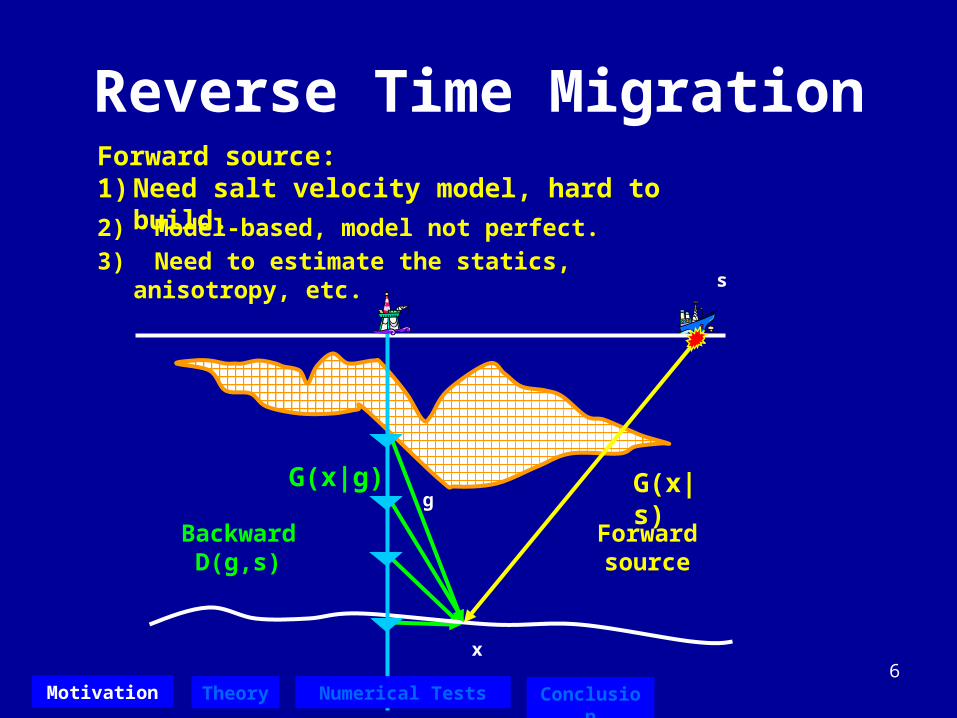
Reverse Time Migration
s
x
G(x|g) g
G(x|s)
BackwardD(g,s)
Forwardsource
Motivation Theory Numerical Tests Conclusion
Forward source:1) Need salt velocity model, hard to build.
2) Model-based, model not perfect.
3) Need to estimate the statics, anisotropy, etc.

7
s
g
g’
x
VSPSWP Interferometry
Migrate virtual source gather D(g|g’) Limitation:
1) s and x are at different side;2) Image near vertical structures;
Motivation Theory Numerical Tests Conclusion

8
Outline
Motivation Theory Numerical Tests Conclusions
Motivation Theory Numerical Tests
Sigsbee VSP data set GOM VSP data set
Conclusion

9
Local Reverse Time Migration, Key Idea
(a) VSP data: P(g|s)=T(g|s)+R(g|s)
Transmission T(g|s)
s
g
Reflection R(g|s)
x
TheoryMotivation Theory Numerical Tests Conclusions

10
Local Reverse Time Migration, Key Idea(a) VSP data: P(g|s)=T(g|s)+R(g|s)
T(g|s)
s
gR(g|s)
x
s
(b) Backward reflection
R(g|s)g
x
R(x|s)= G(x|g)*R(g|s)g
(c) Backward Transmission
T(g|s)
s
g
x
T(x|s)= G(x|g)*T(g|s)
g
(d) Crosscorrelation:
m(x)= R(x|s)*T(x|s)g
TheoryMotivation Theory Numerical Tests Conclusions
Local VSP Green’s function
R(g|s)g
x

11
m(x) ~ s
~ dsg’
G(x|g’)* D(g’|s) dg’
Backward D(g’|s)
G(x|g)* D(g|s)dg
Backward D(g|s)
g
*
x1(1)
(2)
x2
x3
(3)
s
g
g’
Illumination Zones
(1) specular zone, (2)diffraction zone, (3) unreliable zone,
TheoryMotivation Numerical Tests Conclusions
12
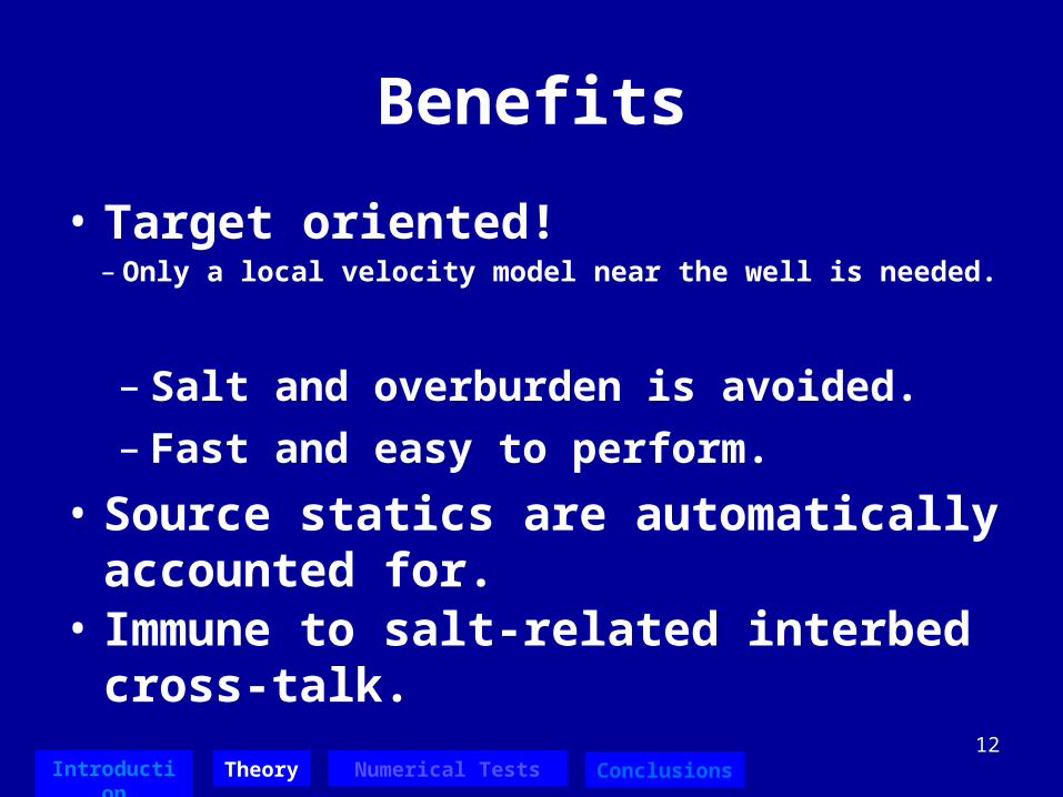
Benefits
• Target oriented!
Introduction Numerical Tests
– Only a local velocity model near the well is needed.
– Salt and overburden is avoided.
– Fast and easy to perform.
• Source statics are automatically accounted for.
• Immune to salt-related interbed cross-talk.
Theory Conclusions

13
Outline
Motivation Theory Numerical Tests Conclusions
• Motivation
• Theory
• Numerical Tests– Sigsbee VSP data set– GOM VSP data set
• Conclusion

14
Sigsbee P-wave Velocity Model0
Dep
th (
km)
9.2
4500
1500
m/s
-12.5 12.5Offset (km)
279 shots
150 receivers
Motivation Theory Numerical Tests Conclusions

15
Local Reverse Time Migration Results
4.6
9.2
Dep
th (
km)
-3 3Offset (km)
True modelMigration image
f = fault
f
d
d
(1)
(2)
(3)
(1) specular zone (2) diffraction zone(3) unreliable zone
d = diffractor
Motivation Theory Numerical Tests Conclusions
16
Outline
Introduction Theory Numerical Tests Conclusions
Motivation Theory Numerical Tests
Sigsbee VSP data set GOM VSP data set
Conclusion

17
Dep
th
(m)
Offset (m)4878
0 1829
0
GOM VSP Well and Source LocationSource @150 m offset
Introduction Theory Numerical Tests Conclusions
2800 m
3200 m
Salt
82 receivers

18
P-to-S ratio = 2.7
Velocity ProfileS WaveP Wave
Dep
th
(m)
0
45000 5000 0 5000
2800 m
3200 m
Salt
GOM Data
Incorrect velocity model
P-to-S ratio = 1.6
Introduction Theory Numerical Tests Conclusions
Velocity (m/s) Velocity (m/s)

19
Z-Component VSP DataD
epth
(m
)
Traveltime (s)
2652
3887
1.2 3.0
Salt
Direct P
Reflected P
Reverberations
Introduction Theory Numerical Tests Conclusions

20
X-Component VSP DataD
epth
(m
)
Traveltime (s)
2652
3887
1.2 3.0
Salt
Direct P
Reflected P
Reverberations Direct S
Introduction Theory Numerical Tests Conclusions
21
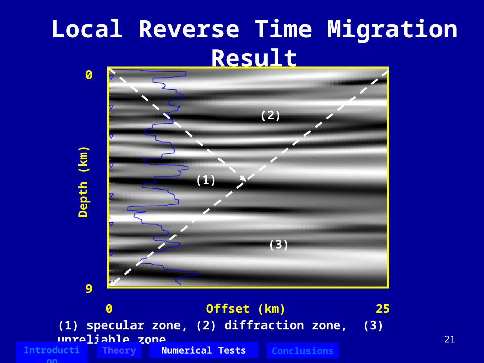
Local Reverse Time Migration Result
(1)
(2)
(3)
(1) specular zone, (2) diffraction zone, (3) unreliable zone
0D
epth
(km
)
9
0 25Offset (km)
Introduction Theory Numerical Tests Conclusions

22
Conclusions
• Target oriented!
Introduction Theory Numerical Tests Conclusions
– Only local well model is needed.
– Salt and overburden is avoided.
– Fast and easy to perform.
• Source statics are automatically accounted for.
• Immune to salt-related interbed cross-talk.

23
Thank you!
• Thank the sponsors of the 2007 UTAM consortium for their support.

24
VSP WEM0
Dep
th (
km)
90 25Offset (km)
SSP WEM 0
Dep
th (
km)
9

25
s
s
x
G2
s
(a) Approximate G2
x
G1 gForwardwavelet
(b) Compute G1
x
g’ G2
data D(g’|s)Backward
x
G1 g G2
(c) Migrate data D(g|s)
D(g|s)
s
Flow Chart
26
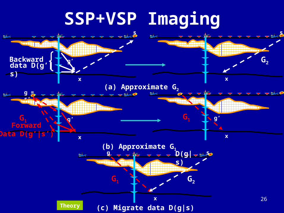
ss
(a) Approximate G2 x
G2
x
g’data D(g’|s)Backward
g = s’
(b) Approximate G1 x
g’
x
g’ G1 Forward
Data D(g’|s’)
G1
x
(c) Migrate data D(g|s)
G1 G2
D(g|s) sg
SSP+VSP Imaging
Theory

27
(b) Backproject reflections
R(x|s)= G(x|g)*R(g|s)g
R(g|s)g
x
28
Outline
Motivation Theory Numerical Tests Conclusions
Motivation Theory Numerical Tests
Sigsbee VSP data set GOM VSP data set
Conclusions