Local Protectionism, Market Structure, and SocialWelfare: China’s Automobile Market

Panle Jia Barwick Shengmao Cao Shanjun Li∗

November 2016

Abstract

While China has made great strides in transforming its centrally-planned economy to a

market-oriented economy, there still exist widespread interregional trade barriers, such as poli-

cies and practices that protect local firms against competition from non-local firms. This study

documents the presence of local protectionism and quantifies its impacts on market competition

and social welfare in the context of China’s automobile market, the largest automobile market

in the world. Using a census of vehicle registration records, we show that joint ventures (JVs)

and especially state-owned enterprises (SOEs) command much higher market shares in their

headquarter province than at the national level. Results from a spatial regression discontinuity

analysis at provincial borders and falsification tests suggest that this pattern is not driven by

differences in consumer preference or dealer network, and point to local protectionism such

as subsidies of local brands as the primary contributing factor. We then set up and estimate a

market equilibrium model to quantify the impact of local protectionism, controlling for other

demand and supply factors. Our counterfactual simulations show that local protectionism leads

to significant choice distortions and consumer welfare loss. It also benefits JVs and SOEs at

the expense of more efficient private firms. In the long run, local protectionism could have

important impacts on market structure such as firm entry and exit as well as resource allocation

across regions.

Keywords: Local Protectionism, Regression Discontinuity, Market Equilibrium Model, Welfare

∗Barwick: Department of Economics, Cornell University and NBER (email: panle.barwick@cornell.edu); Cao:Department of Economics, Stanford University (email: shengmao@stanford.edu); Li: Dyson School of Applied Eco-nomics and Management, Cornell University (email: sl2448@cornell.edu). We thank Matt Backus, Steve Coate,Penny Goldberg, Ivan Png, and seminar participates at Arizona State University, Cornell University, Cornell-PennState Econometrics and IO Conference, Federal Trade Commission, Indiana University, NBER Chinese EconomyWorking Group, New York IO Day Conference, Peking University, University of California-Davis, and University ofWisconsin for helpful comments. We acknowledge generous data sharing from Tao Chen, Rui Li and Xiaobo Zhangand excellent research assistance from Binglin Wang and Jingyuan Wang.

1 Introduction

Since the implementation of market reform and open-up policy in 1978, China has made greatstrides in transforming its centrally-planned economy to a market-oriented economy. By recog-nizing private ownership, unleashing entrepreneurial spirit, and promoting international trade, thereform has led to a phenomenal economic growth with an annual GDP growth rate of 10 percentfor over 35 years.1 Despite the tremendous progress made in integrating with the world econ-omy, China’s domestic market still exhibits widespread interregional barriers to trade. One suchbarrier includes policies and practices that protect local firms against competition from non-localfirms, which we characterize as local protectionism. Local protectionism manifested in these tradebarriers arises from a combination of factors: the top-down political personnel system that reliesheavily on local GDP growth for promotion, rent-seeking behaviour of local officials, and the lackof effective regulations from the central government.

Distortionary polices and practices that affect factor allocation in the input market are docu-mented in both developed and especially developing countries (Banerjee and Munshi, 2004; Peekand Rosengren, 2005; Hsieh and Klenow, 2009). Studies have shown that these policies and prac-tices could have substantial effects on productivity and aggregate output (Baily et al., 1992; Restuc-cia and Rogerson, 2008; Brandt et al., 2009). Our study documents the presence of local protec-tionism and quantifies its impacts on market competition and social welfare in an output market, theautomobile market in China. Discriminatory policies and practices imposed by local governmentschange the relative prices of products based on their origin of production. This in turn distortsconsumer choices, affects how resource and production are allocated across automakers, and haslong-term impacts on market structure and economic performance. Recent policy discussions, inthe midst of slowing Chinese economy, have focused on strengthening domestic demand to promotefuture economic growth. Understanding the impact of local protectionism (and interregional tradebarriers in general) on market competition and social welfare could have important implications forfuture policies.

Using a census of registration records at the individual vehicle level from 2009 to 2011, we doc-ument that vehicle models produced by state-owned enterprises (SOEs) and joint ventures (JVs)command a much higher market share in their headquarter province than at the national level, aphenomenon that we call ‘home bias’. We first present evidence that home bias survives controlsfor consumer demographics, distance and transportation costs, dealer networks, and a variety ofgeographic and temporal fixed effects. To test whether the home bias is driven by consumer pref-erence, we employ a spatial regression discontinuity design by focusing on the clusters of adjacent

1This process was unfolded in three major waves: the reform in the agricultural sector that started in 1978 and madefarmers residual claimants, the privatization of State-own Enterprises (SOEs) from the late 1980’s, and the entry toWTO in 2001, respectively.

2

counties on different sides of provincial borders. We show that strong home bias persists withinthese county clusters: even though counties within a cluster have similar culture, customs, con-sumer demographics and access to dealer stores, SOE and JV products command much highermarket shares in counties located in their headquarter province than in the adjacent counties acrossthe province border. In contrast, home bias is absent for models produced by private automakers, apattern that is robust across various specifications. A consumer survey of recent Chinese car buyersshows that few consumers can distinguish between private or SOE products. These results suggestthat the home bias we have documented is not chiefly driven by either consumer demographics orconsumer ethnocentrism (such as pride and voluntary support for local products), since we controlfor the former by focusing on clusters of similar counties, and the later would have led to a similarhome market advantage by the private firms. Our falsification tests show that non-local productsthat are most similar in attributes to local SOE or JV products do not enjoy any sales advantage inlocal products’ home market. In addition, there is no systematic differences in consumer preferencein adjacent counties across the borders of non-producing provinces (provinces that do not have anyauto firms). Together these results suggest that local protective policies and practices instead ofconsumer preference heterogeneity are the key driver behind our finding. While it is impossibleto obtain an exhaustive list of such policies, we have uncovered a series of them that are targetedtoward SOE and JV products (see section 2 for more details).

To understand the impacts of local protectionism on market competition and social welfare, weset up and estimate a market equilibrium model in the spirit of Berry et al. (1995), incorporatinglocal protectionism as a price subsidy on local products. Demand parameters are estimated usingprovincial-level sales data (macro-moments) and a household survey of new vehicle buyers (micro-moments). First, the estimation results suggest that local protectionism (including explicit subsidiesand implicit barriers) is equivalent to a price discount of 28% for SOE products and 11% for JVproducts, which leads to a sales increase of about 277.1% for SOEs and 44.5% for JVs in theirheadquarter province. Second, estimated subsidies and other preferential treatment amount to 34billion Yuan from 2009 to 2011. Counterfactual simulations show that choice distortions inducedby local protectionism lead to a consumer welfare loss of 12.3 billion Yuan (nearly $2 billon)during the three years of our sample, while industry profit and tax revenue increase by 8 billionYuan due to the subsidies. In addition, these policies lead to substantial redistribution: they benefitaffluent car buyers at the expense of less wealthy consumers and benefit high-cost SOEs and JVsat the expense of more efficient private automakers. Note that our estimates are conservative: theydo not take into consideration the additional social cost that is associated with collecting taxes tofinance these subsidies, exclude institutional purchase (cars procured by local governments and taxicompanies, etc.) that is subjected to local protection, omit subsidies that auto firms receive duringthe production process (subsidy on capital and R&D, tax exemptions, etc.), and ignore long-term

3

consequences of local protection. The aggregate welfare loss associated with local protection inthe passenger car sector of the auto industry could be much bigger than the one presented here.

Our study makes the following three contributions to the literature. First, it adds to the literatureon understanding brand preferences and market share dynamics. Bronnenberg et al. (2012) showthat brand preferences based on past experience are highly persistent and can explain a large percentof geographic variation in market shares. Schmalensee (1982) and Sutton (1991) examine marketshare dynamics in the temporal dimension and illustrate that early entrants can gain a persistentcompetitive edge through consumer learning and advertising.

In the automobile market, the most closely related papers include Goldberg and Verboven(2011) and Cosar et al. (2016). The former studies the integration of the European market andprovides evidence of home bias in vehicle demand across European countries. The latter uses sim-ilar data from six European countries, Brazil, Canada, and the US and concludes that consumerpreference for domestic brand, rather than supply-side considerations, is the main contributing fac-tor to home bias. Our study adds to this literature by showing that local governments’ policies andpractices could be another important factor in shaping the geographic variation in market shares.

The automobile market in China provides a unique setting to study the formation of brand pref-erences that is different from the studies cited above, because most vehicle buyers are first-timeconsumers of cars. The literature on the persistence of demand preference suggest that protectivepolicies could have long lasting effects. Even if these policies are eliminated as China embracesmore reforms and emulates practices in developed countries, they could still affect future marketshare dynamics through persistent brand preference. Our welfare estimates could be vastly under-estimating the long-term efficiency loss induced by these policies.

Second, our paper contributes to the literature on understanding the sources of resource mis-allocation and its implications on productivity and economic growth. Fajgelbaum et al. (2016)examine the impact of state taxes on spatial resource misallocation and show that equalizing statetaxes can increase worker welfare and aggregate output. Hsieh and Klenow (2009) document amuch larger dispersion in the marginal product of capital and labor across firms in China and Indiathan those observed in the U.S.. Brandt et al. (2009) estimate that the distortions in factor allocationin China reduce aggregate TFP by about 30% on average from 1985 to 2007, with the within- andbetween-province distortions accounting for similar portion of the reduction. These studies havefocused on the input market and argued that financial and labor market imperfections could limitthe free flow of capital and labor. Different from the previous literature, our analysis focuses on themarket frictions induced by government policies in a product market. We show that such frictionsincrease the market power of some firms at the expense of others, resulting in inefficient productionallocation and ultimately misallocation of inputs across heterogeneous firms.

Third, our paper adds to the emerging literature on understanding intra-national trade barriers

4

and spatial patterns of production specialization. Within the trade literature, recent studies havequantified the importance of geography in trade costs using data from both developing and devel-oped countries (Anderson et al., 2014; Atkin and Donaldson, 2016; Cosar and Fajgelbaum, 2016).Our paper points to local discriminatory policy as another source of trade costs. These protectivepolicies against non-local firms are hard to measure since they vary across space and time and areoften implicit. Using province level industry aggregate output, previous studies have provided ev-idence of local protectionism by detecting regional specialization that deviates from comparativeadvantage of input factors (Young, 2000; Bai et al., 2004; Holz, 2009). Our study documents localprotectionism in a consumer good industry by showing that local products enjoy home bias thatcannot be explained by transportation cost, sales network, and preference heterogeneity. More im-portantly, our paper is the first to quantify the impacts of local protectionism on market outcomesand social welfare, an important step toward understanding the market structure in an emergingeconomy.

The rest of the paper is organized as follows. Section 2 presents an overview of the automobileindustry in China, discusses the institutional background and anecdotal evidence of local protec-tionism, and describes our data. Section 3 provides evidence of local protectionism using a spatialregression discontinuity analysis and establishes local protectionism as the leading explanation forSOE’s and JV’s home bias using falsification tests and a consumer survey. Section 4 sets up amarket equilibrium model of vehicle demand and supply and discusses the identification strategy.Section 5 presents results from the structural model. Section 6 conducts simulations to quantify thewelfare impact of local protectionism. Section 7 concludes.

2 Background and Data

In this section, we first present anecdotal evidence of local protectionism and discuss the relevantinstitutional background. We then provide an overview of China’s automobile industry and describethe data.

2.1 Local Protectionism

We define local protectionism as policies and practices that protect local firms against competitionfrom non-local firms. In the automobile market, a common practice is to give consumers directsubsidies or tax incentives for purchasing local products, where the definition of a “local” productis tied with different requirements across jurisdictions.2

2Yu et al. (2014), an article in Wall Street Journal on 5/23/2014, reports that government subsidy to 22 publicly tradedautomakers in China amounted to 2.1 billion Yuan in 2011 and this number increased to 4.6 billion in 2013. Thearticle acknowledges that “(t)he subsidies come in many forms, including local government mandates and subsidies

5

Table 1: Examples of Local ProtectionismCase From To Location Size Eligibility1 3/1/09 12/31/09 Hebei 10% or 5000 Local minivans2 7/1/09 12/31/09 Heilongjiang 15% or 7500 Local brands3 8/18/09 unkown Henan 3% or 1500 Local brands in Henan4 1/1/12 12/31/12 Chongqing total 300mil. Changan Automotive5 4/4/12 12/31/12 Anhui 3000 Local brands for Taxi6 7/1/12 6/30/13 Changchun, Jilin 3500-7000 FAW indigenous brands7 1/1/14 12/31/14 Chongqing total 70mil. Changan Automotive8 4/16/14 unkown Xiangtan, Hubei 2000 Geely Automotive9 5/1/15 4/30/16 Fuzhou, Jiangxi 5%-10% Jiangling Automotive10 11/15/15 12/15/15 Guangxi 1500-2000 Local brands

Source: Official government documents from online searches. Unit in Yuan.

From online searches with the keywords ”subsidy + promote automobile industry”, we compilea list of policies in the past few years that subsidize buyers of local brands using direct mone-tary transfer, tax and fee waivers, or low-interest loans. Table 1 presents ten cases of subsidywith explicitly stated compensation amount for products that are produced either by designatedlocal automakers or in the jurisdiction. The 6th case is worth noting in that the subsidy only ap-plies to indigenous brands produced by the state-owned subsidiaries of the First Auto Works group(henceafter FAW), but not to the brands by the JV subsidiaries of FAW.3

Besides direct subsidies, local protectionism comes in many other forms: explicit requirementsfor government agencies and taxi companies to purchase local brands; procurement priority ortailpipe emission standards that favor local brands; and explicit and implicit barriers for non-localbrands to establish dealer network. The common theme of the stated rationale behind these poli-cies in official government documents is to increase employment, strengthen the local automobileindustry and in turn the local economy.

It is important to note that the local protectionism or various trade barriers more generallythat we analyze here is not about physical barriers related to a poor transportation infrastructure.Highways, the railway systems, as well as supply chain management have improved dramaticallyin China during the last decade (Faber, 2014).

Local protectionism in China arises from a combination of factors. First, market reforms startedin 1978 made economic development the primary responsibility for local governments. GDPgrowth became an essential measure of performance in the top-down political personnel systemwhere local officials (provincial governors, city and county mayors) are evaluated by government

for purchases of locally made cars, making a total figure for local and national financial help difficult to calculate.”3FAW is one of the largest automakers in China. It has three state-owned subsidiaries producing indigenous brandssuch as Besturn and three JV subsidiaries producing Volkswagen, Toyota, and Mazda models.

6

officials at the higher level.4 In addition, the fiscal decentralization whereby local expendituresare mostly financed by local revenue provides officials incentives to seek a strong local economy(Jin et al., 2005). Both the promotion system and fiscal decentralization lead to inter-jurisdictionalcompetition and discriminatory policies that protect local firms against competition from non-localfirms.

A famous example is the ‘war of license fees’ between Shanghai and Hubei province in thelate 1990s. Starting from the early 1990s, Shanghai municipal government implemented ReservePrice auctions for vehicle license plates. Vehicle buyers were required to pay for the license platebefore registering their newly purchased vehicles. In 1999, in the name of promoting the growth oflocal automobile industry, Shanghai government set the reservation price to 20,000 yuan for localbrands (e.g. Santana produced by Shanghai Automotive) and 98,000 yuan for non-local brands.In retaliation, Hubei province, the headquarter province of China’s Second Automotive Group,charged an extra fee of 70,000 yuan to Santana consumers “to establish a fund to help workers ofcompanies going through hardship” .

Second, local government officials often derive private benefits from local SOEs and JVs. Localgovernments appoint the top executives of SOEs and JVs in their jurisdiction and there exists arevolving door between top executives in these companies and government officials. A a result,local government officials can directly benefit from local SOEs in many ways, ranging from findingjobs for their relatives in these companies to eliciting monetary support for public projects and evenprivate usage.5

Third, the central government has not been very effective in regulating inter-regional trades.While the literature of fiscal federalism points out the potential benefit of allowing local govern-ments to make better-informed decisions on public goods provision, it also acknowledges the pit-falls of regional protectionism and allocative distortions (Oats, 1972). The central governmentplays an important role in addressing these pitfalls through promoting a national market and elim-inating trade barriers. The Commerce Clause in the U.S. Constitution explicitly prohibits stateregulations that interfere with or discriminate against interstate commerce. This to a large extentfrees the U.S. market of local protective policies observed in China, although some inter-state tradebarriers also persist in the U.S. (Fajgelbaum et al., 2016). Although China’s Anti Unfair Compe-tition Law, passed in 1993, explicitly prohibits municipal or provincial governments from givingpreferential treatment to local firms, enforcement of the law has not been very effective.

As Table 1 shows, local protectionism often manifests as differential treatment for firms withdifferent ownership types. SOEs are treated most favorably because of their importance in the lo-

4The effectiveness of the one-child policy used to be an important criterion. In recent years, environmental measuresare added to the evaluation system.

5This has been highlighted by many recent high-profile corruption cases in China where government officials wereconvicted of taking eye-popping bribes from executives of large companies in their jurisdiction.

7

cal economy and close ties between SOE top executives and local government officials. JVs liebetween SOEs and private firms in the spectrum of differential treatment. By law, JVs are ownedin majority by Chinese automakers and in practice, the Chinese partners are all SOEs. In the em-pirical analysis, we measure the degree of local protection for SOEs, JVs, and private automakersseparately. Consistent with Bai et al. (2004) which finds stronger local protectionism in industrieswhere SOEs account for a larger output share, our empirical analysis shows that local protectionismbenefits SOEs the most and JVs the second.

2.2 The Chinese Automobile Industry

Like many other industries, China’s automobile industry rose from virtually non-existent thirtyyears ago to the top of the world at an astonishing speed. Figure 1 depicts the annual sales of newpassenger vehicles in U.S. and China. The total number of new passenger vehicle sales in Chinaincreased from 0.85 million in 2001 to 21.1 million in 2015, surpassing the U.S. to become thelargest market in the world in 2009. The growth in China’s automobile market during this periodaccounted for about 75 percent of the growth in the world automobile market.

Figure 1: New Passenger Vehicle Sales in China and U.S.

All major international automakers currently have production capacity in China. Following thestrategy of “exchange-market-for-technology”, or “Quid Pro Quo” (Holmes et al., 2015), Chinesegovernment requires foreign automakers to form joint ventures with domestic automakers in orderto set up a production facility. The non-Chinese parties combined in a joint venture cannot claimmore than 50 percent of the ownership. A purpose of such a requirement is to help domestic

8

automakers to learn from foreign automakers and eventually compete in the international market.Volkswagen was the first to enter the Chinese market by forming a JV with Shanghai Automotive in1983. To date, Volkswagen and GM have the largest presence in China among foreign automakers.

For its potentially large contribution to local employment and GDP and its spillover benefitsto upstream industries, the automobile industry is a frequent target for government protection.Provinces compete to provide financial incentives to attract automakers. As a result, automobileproduction currently exists in 26 out of 31 provinces. During China’s 11th Five Year Plan from2005 to 2010, all of these provinces designated the automobile industry as a strategic industry thatenjoy tax benefits and various other government support.

Perhaps not surprisingly, China’s automobile market is much less concentrated and the averageoutput of each automaker is smaller compared to the U.S.. In 2015, there are over 60 automakersproducing in China and the top six dominant firms account for 46% of market shares. After years ofrapid expansion, the Chinese auto industry is plagued with overcapacity, with an average capacityutilization rate of merely 65%. In contrast, in the U.S., there are fifteen automakers and the top sixfirms control 77% of the market. The automobile assembly plants are located in 14 out of 50 states,with an average capacity utilization rate around 85%.6

2.3 Data

Our analysis is based on four main data sets: (1) the universe of individual vehicle registrationrecords from 2009 to 2011 that is compiled by the State Administration of Industry and Com-merce, (2) trim level vehicle attributes from R. L. Polk & Company (henceforth Polk), (3) citylevel household demographics from the 2005 one-percent population survey, and (4) an annualsurvey of new vehicle buyers by Ford Motor Company.

For the vehicle registration data, we observe the month and county of registration, the brandand model name of the vehicle registered, as well as major attributes such as transmission type,fuel type, and engine size. We also observe whether the license is for an individual or institutionalpurchase. Institutional purchases account for about 10% of all registration records. As one mightexpect, institutional purchases exhibit a much greater extent of home bias (appendix C). We focuson individual purchases in this study since institutional purchases are often driven by non-marketconsiderations that require a different model. We aggregate data to the model-county level forthe spatial discontinuity analysis in Section 3, and to the model-province level for the structuralestimation in Section 4. To translate the number of registration records, or sales, into market shares,

6According to a 2013 OECD report titled “Medium-Run Capacity Adjustment in the Automobile Industry”, the capac-ity utilization in China’s automobile industry was 64 percent in 2012, compared to 83 percent in both U.S. and Japanand 84 percent in Germany.

9

we define market size as the number of Chinese households in each province.7 JVs contribute to68.7% of total sales during our sample period. Private automakers, SOEs, and imports account for11.4%, 16.7% and 3.1% of total sales, respectively.

The trim-level vehicle data report the manufacturer suggested retail price (MSRP), vehicle type(sedan, SUV, or MPV), vehicle size (m2), engine size (liter), horsepower (kilowatts), weight (ton),transmission type, and fuel type. MSRPs are set by manufacturers and are the same nationwidefor each model-year. Discounts offered by individual dealers may lead to transaction prices thatare different from the MSRPs. According to a 2016 store-level promotion data that is discussedin detail in Appendix B, there are small regional variations in retail prices.8 However, we believethat MSRP is a decent approximation of transaction price (which we do not observe) in our studyfor two reasons. First, heavy discounts are rare: around 40% of trim-by-store observations have nodiscount, 25% have a 10% discount, and only 3% have a 20% discount. More importantly, dealerstores do not give more discount to local products, which suggests that using MSRP in place of thetransaction price will not bias the estimation of local protection.

MSRP in China includes value-added tax, consumption tax, as well as import tariffs whenapplicable.9 It does not include sales tax, which is normally set at 10% but is reduced to 5% and7.5% for vehicles with engine displacement no more than 1.6 liter in 2009 and 2010, respectively.We add sales tax to MSRP, and deflate it to the 2008 level to obtain the real transaction price paidby consumers. We choose engine size over horsepower-to-weight ratio as a measure of accelerationbecause engine size is known to be a more salient feature for auto buyers in China.

We define a model by its model name, vehicle type, transmission type, and fuel type. Trimlevel attributes are aggregated to the model level via a simple average, and then matched to ourregistration data. Price and attributes for each model are constant across all markets in a given year,but exhibit between-year variations due to price updates, introduction of new trims, and withdrawalof old trims. To construct a measure of fuel economy, we first collect information on the fuel con-sumption per 100km for each model from the Ministry of Information and Industrial Technology(MIIT). Then we multiply it with the province-year gasoline price to obtain the average fuel cost inyuan per 100km.

7While some consumers might purchase a new vehicle in one province and register it in another province, this isuncommon since dealers typically bundle services with the sale price of a new vehicle.

8We collect the promotion data from Autohome.com, a major privately-run gateway website that regularly updatesinformation on car features and industry headlines. Minimum Retail Price Maintenance (RPM) whereby automakersprohibit dealers from selling below a preset price has been common in China. For example, the China AutomobileDealers Association complained in 2011 that large automakers had been imposing RPM and exclusive territory toreduce price-competition among dealers. This did not draw attention from China’s antitrust authority until veryrecently. As in the U.S., RPM is not treated as per se illegal by China’s antitrust authority and each case has to bejudged based on individual merits.

9Consumption tax is levied to promote sales of small and fuel-efficient vehicles. It varies from 1% to 40%, dependingon vehicle size.

10

Besides prices and attributes, another important factor for auto demand is the dealer network.Due to the lack of historical data, we use a cross section of dealer counts by brand and province inMarch 2016 to approximate the dealership network during our sample period. According to reportsby China Auto Dealers Association (CADA), the number of dealer stores in China increased from13,000 in 2009 to 24,000 at the end of 2014. Appendix A shows that automakers have a moreextensive dealer network in their home market than in other provinces, but the differences are notas large as those observed in sales, suggesting that dealer network only partially explains the homebias in sales.

Information on headquarter and plant locations is obtained from each firm’s website. Our finalconsists of 38 domestic firms and 14 foreign firms. The domestic firms include 6 private firms, 20JVs, and 12 SOEs. No firm moved its headquarter within our sample period, and only two openednew plants. For each model produced by a domestic firm, we find the commuting distance betweenits plant location and each of its destination markets.

Our raw dataset contains a total of 683 models. Many of them are only sold in a few provinceswith very low sales. We keep the most popular models that account for 95% of national sales ineach year. Doing so has several benefits. First, sales of small brands are likely measured with errors.Second, and more importantly, since we focus on analyzing differences between vehicle models’local shares and national shares, limiting to major national brands gives us a conservative measureof local protectionism. For example, some brands might not be marketed nationally. Including themin our analysis would exaggerate the extent of local protection. Third, obtaining counterfactualequilibrium prices is computationally challenging when we have a demand system with a largenumber of products. We also drop models priced above 800,000 RMB (about $123,000), as demandfor these luxury brands is likely driven by conspicuous consumption or other factors not capturedin our stylized model. That leaves us with a total of 179, 218, and 234 models in each year. Choicesets across provinces in any given year do not vary much. For example, in 2011, 25 out of 31provinces have all 234 models. The choice set does exhibit variation over time, due to entry andexit of vehicle models. The total number of observations in our final sample is 19,505.

11

Table 2: Summary Statistics of Key VariablesVariable Mean Std. Dev. Min MaxSales 1259 2263 1 60612Real price (1000 yuan) 184.7 144.5 27.5 798.7Fuel cost (yuan/100 km) 50.1 10.0 24.9 101.2Engine size (liter) 1.8 0.5 0.8 4.0Vehicle size (m2) 7.7 0.9 4.2 10.3Auto transmission 0.48 0.50 0 1SUV 0.17 0.37 1 0MPV 0.06 0.24 0 1Number of dealers 20.8 23.3 0 137Distance to headquarter (1000km) 2.1 1.4 0 5.2Note: The number of observations is 19,505. Sales are monthly sales by model andprovince. The number of dealers is by province and brand.

Table 2 reports the summary statistics. The average price of a vehicle is 184,700 Yuan (about$28,000). The average price is similar to that observed in the U.S. market but the price range islarger in China. The indigenous brands from domestic automakers tend to occupy the low-endsegment while the JVs and imports compete in the high-end segment. Among the brands from JVsand imports that are also available in the U.S. market, our price comparison shows that the pricesfor entry models (such as Ford Focus and Toyota Corolla) are similar in the two markets but thosefor luxury brands can be twice as expensive in China as in the US. The price difference for thesevehicles can be attributed to the high consumption tax (as high as 40% of the wholesale price), thenature of demand (e.g., conspicuous consumption), and market competition (Li et al., 2015).

Table 3 below shows that different types of firms have very different product mix. JV brandson average have a higher price, vehicle size, and engine size compared to private or SOE brands.The price difference between JV products and their domestic counterparts is much larger than thedifference in the observed attributes. Higher prices are largely driven by better brand recognitionand higher unobserved qualities, which we capture using brand fixed effects in our estimation. Inaddition, JVs have a more extensive dealer network, and a larger fraction of their products haveautomatic transmission. Imported products are typically luxury brands, and majority of them areSUVs.

12

Table 3: Mean values of Key Variables by Firm TypeVariable Private JV SOE ImportsSales 1271 1443 1118 382Real price (1000 yuan) 80.0 188.3 96.0 428.1Fuel cost (yuan/100 km) 45.7 49.7 47.7 61.7Engine size (liter) 1.5 1.8 1.6 2.5Vehicle size (m2) 7.2 7.9 7.4 8.3Auto transmission 0.06 0.55 0.17 1SUV 0.20 0.11 0.10 0.56MPV 0 0.04 0.15 0.11Number of dealers 13.1 26.3 11.6 12.0Number of observations 2230 11907 3363 2005Note: Sales are monthly sales by province. The number of dealers is byprovince by brand.

Rising household income is perhaps the most important factor that drives China’s exponentialgrowth in vehicle sales since the mid 2000s. To account for the impact of income on vehicledemand, we obtain empirical distributions of household income at the province level from China’s1% population survey in 2005, separately for urban and rural households. Such comprehensivedata at the individual level or county level for recent years are difficult to find. Consequently, foreach year in our sample period, we scale each provincial income distribution from the 2005 surveysuch that its mean matches the provincial average from the annual China Statistical Yearbooks.10

By using the 2005 census data, our implicit assumption is that the shape of income distributions inChina did not change significantly between 2005 and 2011.

Besides the income distribution for the general population, we also obtain the income distri-butions for new vehicle buyers from an annual survey conducted by Ford Motor.11 The surveybreaks annual household income into four brackets: less than 48k Yuan, 48k-96k Yuan, 96k-144kYuan, and greater than or equal to 144k Yuan, and reports the fraction of vehicle buyers from eachincome bracket in each year. It further divides vehicles into 24 types and reports the fraction ofcar buyers in each income bracket for each vehicle type. We aggregate the 24 types into five seg-ments: mini/small sedan, compact sedan, medium/large sedan, sport utility vehicle (SUV), andmulti-purpose vehicle (MPV).

The first panel of Table 4 compares the income distribution among all vehicle buyers to that ofthe general population. The second panel of Table 4 reports the income distribution of consumersfor each of the five vehicle segments in 2011. Consumers with a higher household income aredisproportionately more likely to buy new vehicles, especially high-end sedans, SUVs, and MPVs.In 2011, only 4% of households in China have annual income above 144k, which is the median10In 2010, the average household income in China is about one seventh of that in the U.S..11The survey covers 20,293, 22,915, and 33,961 vehicle buyers in 2009, 2010, and 2011, respectively.

13

Table 4: Micro-moments: Fraction of Vehicle Buyers by Annual Income

(a) Fraction of Households by Annual Income (yuan)

Year < 48k 48k−96k 96k−144k ≥ 144kAmong Vehicle Buyers2009 0.16 0.34 0.32 0.192010 0.11 0.27 0.32 0.302011 0.09 0.26 0.34 0.31

Among All Households2009 0.69 0.23 0.05 0.032010 0.63 0.27 0.06 0.042011 0.55 0.33 0.08 0.04

(b) Fraction of Buyers by Income Brackets for Different Vehicle Segments, 2011

Segment < 48k 48k−96k 96k−144k ≥ 144kSmall/mini sedan 0.15 0.40 0.30 0.15Compact sedan 0.11 0.30 0.37 0.22Medium/large sedan 0.05 0.16 0.32 0.47SUV 0.05 0.15 0.33 0.47MPV 0.07 0.24 0.33 0.36

price of a car in our sample. Yet they account for 47% of the sales of medium/large sedans andSUVs, and 36% of MPVs. The information on consumer income distribution is used to form micro-moments in our estimation as in Petrin (2002) and helps us to separately identify price elasticityand income elasticity.

3 Descriptive Evidence and Spatial Discontinuity

We first provide descriptive evidence on the strong home bias enjoyed by JVs and especially SOEs.Then we use a spatial regression discontinuity analysis and a series of falsification tests to showthat local protectionism is the leading cause of home bias.

Home bias is well documented in the trade, finance, and marketing literature (French andPoterba, 1991; McCallum, 1995; Klein and Ettensoe, 1999). It is typically though not exclu-sively observed in the international context with respect to products from different countries (e.g.,a country-of-origin effect). Our analysis focuses on interregional trade and the home bias we studyis a province-of-origin effect (based on vehicle assembly) within a country.

14

3.1 Descriptive Evidence

To graphically illustrate differences in sales between the home province and the national market,Figure 2 contrasts the market share at the national level with that in the headquarter province for se-lected automakers. The first four are private automakers, the next five JVs, and the last five SOEs12.For non-private firms, especially SOEs, market shares in their local market are significantly higherthan those at the national level. One notable example is Xiali: it accounts for only 2.36% of na-tional new vehicle sales but enjoys a market share of 16.4% in its home province Tianjin. Thereis no noticeable home bias for most private automakers. Appendix A provides the comparison fora comprehensive list of automakers: across the board, SOEs exhibit the strongest home bias andprivate automakers the least.

Figure 2: National and Home-Province Market Shares

0%

5%

10%

15%

20%

25%

30%

Local share National share

Besides local protectionism as we discussed in Section 2.1, there are a number of reasons thatcould to lead to this disparity. First, transportation costs are lower in the local market. However,transportation costs do not have an impact on demand unless they are reflected in vehicle prices.MSRP is the same across all markets for each model in our sample, and our promotions data donot show any appreciable difference between dealer discounts in local and non-local markets. Thissuggests that firms are absorbing the higher transpiration costs (they typically account for one totwo percent of vehicle prices) in markets further away from their production facilities instead ofpassing them through to consumers. Nonetheless, vehicle demand could depend on distance since

12For each firm type, we select firms that have the largest national market shares. These twelve firms together accountfor over 60% of total vehicle sales in China between 2009 and 2011.

15

nearby consumers have better information about a product and greater exposure to local advertising.In this section, we focus on counties that border with each other and hence have similar distancesto the production facilities. In the structural analysis in the next section, we control the distancebetween the production location and the destination market.

Second, appendix A shows that brands produced in the home province have more extensivedealer networks. However, the differences in dealer network between the national market and thehome market are typically smaller than those in sales. In our analysis, we control for the numberof dealers by brand either by focusing on adjacent counties or including the number of dealersby brand in the regression explicitly. It is worth noting that the observed differences in dealernetwork could be partly driven by local policies and practices that treat dealers of local brandsmore favorably in the process of issuing dealer license permits.

Third, there could be a better compatibility of consumer preference and local products. Forexample, many JVs have headquarters in high-income markets such as Beijing, Shanghai, andGuangdong, and sell expensive foreign brands that are popular among wealthy households. Simi-larly, SOEs that produce low-priced indigenous brands tend to locate in less wealthy provinces suchas Anhui, Jilin, and Liaoning. The better match between household income in the home market andthe market segment could lead to larger market shares locally than nationally for these products,as documented in Cosar et al. (2016). We include income, arguably the most important householddemographics, in our analysis in addition to a variety of fixed effects such as provincial fixed ef-fects, and their interaction with vehicle type. In addition, we conduct falsification tests below andthe results suggest that this is unlikely to be an important factor.

Fourth, there could exist an innate preference for locally produced vehicles due to consumerethnocentrism whereby consumers in one group (typically a country) may view purchasing prod-ucts from another group being inappropriate or maybe even immoral because doing so could hurtlocal economy or for other considerations(Shimp and Sharma, 1987). Consumer ethnocentrismor animosity could give rise to the country-of-origin effect and is well studied in the marketingliterature (Klein and Ettensoe, 1999; Canli and Maheswaran, 2000). It is important to note thatconsumer sentiments such as ethnocentrism is often studied in the context of products from differ-ent sovereign countries, our research focuses on interregional trade within China.

Last, discounts to company employees could also increase local sales.

3.2 Spatial Regression Discontinuity

Using our county-level vehicle sales data, we employ a proof-by-elimination strategy in which wecarefully rule out each of the the five factors discussed earlier as the main driver of home biasin vehicle demand, and thereby identify the effects of local protectionism. Our main empirical

16

strategy is a spatial discontinuity design in which we limit our analysis to clusters of adjacentcounties across provincial borders. We focus on provinces that house headquarters of automakersand group counties into different clusters, each of which contains two or three adjacent counties ondifferent sides of a provincial border. We leave out counties along the borders of Tibet, Xinjiang,and Qinghai, since these counties are too large for our identification assumptions. Our final sampleconsists of 630 counties in 285 clusters as shown in different color in Figure 3.

Figure 3: Clusters of Counties along Provincial Borders

The spatial discontinuity design takes advantage of the fact that provincial borders lead to dis-continuity in the types of protective policies and practices discussed in Section 2.1, while assumingsimilar consumer preference across the borders. We focus on the differences within each clusterand control for cluster-specific preferences for different brands, e.g., one cluster of counties mayprefer SUVs over sedans due to road conditions. The underlying assumption is that because of thegeographic proximity, consumers within the cluster have similar taste for vehicles (i.e., no disconti-nuity at the border) and similar access to information and dealer stores . The key empirical patternof interest is whether the differences in market shares persist within each cluster, that is, whetherbrands sell much better in a county within the home province than the nearby county across theborder. We focus on the standard RD regressions in this section and provide further supportingevidence through falsification tests and intra-province analysis in next section.

We implement the spatial discontinuity design in the logit framework using county-level sales

17

data following Berry (1994):

ln(s jm

s0m) = β1HQ jmPRI j +β2HQ jmJV j +β3HQ jmSOE j

+γ1PL jmPRI j + γ2PL jmJV j + γ3PL jmSOE j

+φ jc(m)+δm +ηt +ξ jmt , (1)

where s jm stands for the market share of product j in county m, and s0m stands for the share of theoutside option. Cluster-model fixed effects, φ jc(m), control for differences in consumer preferencesacross clusters. The implicit assumption is that consumers in counties within the same cluster havethe same preference for each model. After further controlling for county fixed effects and year fixedeffects, we identify our parameters of interest, β1 to β3, from the difference in market shares byfirm type between home-market and non-home-market counties within the same cluster. We alsolook at whether plant presence in some non-home-province leads to an increase in demand. 13

The spatial discontinuity design tests whether observed home bias survives after controllingfor a number of confounding factors discussed above. More specifically, it controls for distance,dealership network, and to a limited extent consumer demographics. Within the same cluster, eachbrand has similar market access to all counties since it is easy to commute to a dealer located in anadjacent county.14

Table 5 summarizes the results. Columns (1) and (2) control for model fixed effects. Column(1) includes all 2336 counties in our full sample, while column (2) only includes the 630 countiesalong provincial borders. Results in columns (1) and (2) are similar, indicating that the magnitudeof home bias does not differ significantly in the set of bordering countries from that in the fullsample. Home advantage for private products is negative but small in column (1) and statisticallyinsignificant across all other specifications. The estimates of β1 and β2 reflects the captures of homebias: sales for JVs and SOEs in their home markets are higher by 82% and 180%, respectively.

Columns (3) and (4) implement the spatial discontinuity design by including cluster-modelfixed effects following the identification strategy described earlier. Column (4) restricts the sampleto 373 counties that have similar GDP per capita within a cluster. The home bias for JVs and SOEsonly reduces moderately from column (2): down from 82% to 52% for JVs and from 180% to 159%for SOEs in column (3). Results in columns (3) and (4) are very similar. The large β estimatesthat survive the control of cluster-model fixed effects suggest that distance, access to dealers andconsumer demographics are not the drivers of home bias observed in our data. The results alsoshow that SOEs, but not JVs or private automakers, also enjoy higher demand in non-home markets

13PL jm takes value 1 in all counties in a province that is not the headquarter province for model j, but has a plant bythe firm that produces model j.

14When one buys a car in another county, the registration will occur at the county of residence and is recorded so inour data.

18

where they have production facilities.

Table 5: Results from the spatial discontinuity modelAll All Clusters Clusters(1) (2) (3) (4)

HQ*Private, β1 -0.16*** -0.00 0.12 0.12(0.04) (0.07) (0.08) (0.11)

HQ*JV, β2 0.68*** 0.60** 0.42*** 0.41***(0.03) (0.06) (0.03) (0.04)

HQ*SOE, β3 1.09*** 1.00*** 0.95*** 0.94***(0.03) (0.05) (0.04) (0.06)

PL*Private, γ1 0.26*** 0.21*** 0.02 -0.08(0.04) (0.07) (0.07) (0.11)

PL*JV, γ2 0.15*** 0.18** 0.03 -0.07(0.02) (0.04) (0.045) (0.06)

PL*SOE, γ3 0.63*** 0.61*** 0.42*** 0.51***(0.04) (0.08) (0.079) (0.08)

County FE Yes Yes Yes YesYear FE Yes Yes Yes YesModel FE Yes Yes No NoCluster-model FE No No Yes YesNo. of counties 2336 630 630 373No. of obs. 885376 180398 180398 96058

Notes: In column (4), we restrict the sample to clusters where theratio between the highest and lowest GDP per capita across coun-ties within the cluster is no larger than 1.6. p<0.1, ** p<0.05, ***p<0.01.

Cosar et al. (2016) document that a country-of-origin effect of 240 percent in vehicle demandbased on data from nine countries. They show that consumer preference for products that areoriginated or assembled from the same country accounts for nearly 70 percent of the home bias,with supply side factors (tariff and trade barriers) and dealer network explaining the rest. In China,imports account for less than 7% of new vehicle sales today, and hence our focus is on vehiclesproduced within China. The home bias in this study captures the province-of-origin (in terms ofassembly) rather than the country-of-origin effect.

We argue that consumer ethnocentrism (an innate preference for local products), the fourthfactor discussed above, is also unlikely to be a significant driver of home bias. Our RD analysisshows that private automakers do not have any appreciable advantage in their home markets whileJVs and SOEs do. For consumer ethnocentrism to be an important factor, one has to argue thatthe innate preference for local brands only applies to SOEs and JVs but not private automakers.There is no reason to believe that this should be the case: few consumers know the differencesin ownership structure, especially between SOEs and private automakers. This is confirmed from

19

a survey of Chinese consumers who recently bought a car. We conducted a pilot study at dealerstores in an affluent province in eastern China that accounts for about 10% of national sales. Ourresults indicate that few car buyers in China can tell whether an auto maker is private or an SOE.A surprisingly low fraction of consumers can recognize a JV, even though all of these firms’ namesprominently feature the name of their foreign partner (e.g. BMW Brilliance).

To examine the impact by employee discount, we look at the degree of home bias at the pro-duction counties, where the company employees are likely to reside. We estimate the followingmodel:

ln(s jm

s0m) = β1HQ jmPRI j +β2HQ jmJV j +β3HQ jmSOE j

+α1OwnPL jmPRI j +α2OwnPL jmJV j +α3OwnPL jmSOE j

+θ1OtherPL jmPRI j +θ2OtherPL jmJV j +θ3OtherPL jmSOE j

+ρ j +δm +ηt +ξ jmt , (2)

OwnPL jm takes value 1 if county m is the production county for model j. OtherPL jm takes value 1if county m is not the production county for model j, but has a plant owned by the firm (it producessome other model by the firm). 17 out of the 38 firms in our sample have production plants in at leasttwo different counties, each of which produces a different set of models. In this specification, weidentify the α and θ parameters by comparing sales in the production counties with other countiesin the same province. Table 6 below shows the estimation results.

Table 6: Home Bias at the production counties(1) (2)

Est. SE Est. SEHQ*Private, β1 -0.17*** 0.04 -0.17 0.04HQ*JV, β2 0.66*** 0.03 0.66*** 0.03HQ*SOE, β3 1.07*** 0.03 1.06*** 0.03OwnPL*Private, α1 0.72*** 0.17 0.68*** 0.18OwnPL*JV α2 0.90*** 0.22 0.91*** 0.22OwnPL*SOE α3 0.92*** 0.32 0.90*** 0.32OtherPL*Private θ1 -0.27*** 0.03OtherPL*JV θ2 0.11*** 0.02OtherPL*SOE θ3 -0.25 0.23No. of obs. 885376 885376No. of counties 2336 2336

Notes: We control for model, county, and year fixed effects.* p<0.1, ** p<0.05, *** p<0.01.

We see significant home bias in the production county, but not in other plant locations by the

20

same firm. Such results suggest that employee discount is unlikely to be a key driver of home bias.Employee discounts typically cover all products under a firm, instead of just the models producedin the plants where the employees work. Therefore, if employee discounts have a large impact ondemand, we should expect positive and significant estimates for the θs.

An interesting result from Table 6 is that models by all three types of firms, including the privateautomakers, have significant home bias in their production counties (in addition to the home biasin the headquarter province). The result suggests that there could be some consumer ethnocentrismnear the production sites15, but it dissipates rapidly once we move out of the production county.

Table 7 below shows results from a specification in which we interact the HQ dummy withdistance from the production county. The unit of distance is 1000 km. The median distance inour sample is 0.16 (160km), while the maximum distance is 0.6 (600km). The reference group iscounties outside the headquarter province.

Table 7: Home bias within the headquarter province

(1) (2)Est. SE Est. SE

HQ*Private, β1 -0.17*** 0.04 -0.14** 0.06HQ*JV, β2 0.66*** 0.03 0.81*** 0.05HQ*SOE, , β3 1.07*** 0.03 1.28*** 0.06OwnPL*Private, α1 0.72*** 0.17 0.70*** 0.18OwnPL*JV, α2 0.90*** 0.22 0.75*** 0.22OwnPL*SOE, α3 0.92*** 0.32 0.71** 0.32HQ*Dist*Private -0.18 0.19HQ*Dist*JV -1.05*** 0.20HQ*Dist*SOE -1.19*** 0.28

Notes: We control for model, county, and year fixed effects.* p<0.1, ** p<0.05, *** p<0.01.

Home bias for models by private automakers completely disappears once we move out of theproduction county, suggesting that consumer ethnocentrism is extremely localized. On the otherhand, home bias for JV and SOE models also drops steeply when we move out of the produc-tion counties, and continues to dissipate slowly as we move further away inside the headquarterprovince. However, a large part of it remains intact even at the maximum distance, where the coef-ficients for JV and SOE are 0.18 and 0.56, respectively. One explanation for the variation in homebias is heterogeneous degrees of local protection within the headquarter province. For example,three of the ten examples of local subsidies in Table 1 are implemented at the prefecture level, andonly applicable to counties in the same prefecture as the production counties. Overall, results from

15Another possible explanation is county-level government protection, which is less likely since our previous resultssuggest no evidence for local protection for the private firms.

21

Table 7 suggest that while consumer ethnocentrism contributes to a large part of home bias at theproduction counties, its impact highly localized and almost completely diluted when we comparesales at the province level.

3.3 Falsification Tests

The spatial discontinuity design allows us to control for cluster-specific consumer preferences,dealer networks, and travel distance by focusing on neighboring counties across provincial bor-ders. The key identification assumption is that there are no systematic differences in consumerpreference toward local SOEs or JVs within the county-cluster, that is, no discontinuity in con-sumer preference across provincial boundaries. This could be violated if, for example, auto makerslocate their headquarter in provinces that better match local consumer demographics (observed andunobserved). Although observed consumer demographics tend to be similar between neighboringcounties across provincial borders, there could be differences in unobserved consumer demograph-ics.16 We conduct the following falsification tests to examine this assumption.

If consumers prefer local products because these products are more compatible with consumerdemographics in the home province (observed and unobserved), we should find a market advantageof non-local products that are similar to local products. Our first falsification test replaces each localmodel with its closest non-local counterpart(s). Specifically, we group the 186 domestic modelsin 2011 into 68 groups of similar models. The models in each group have headquarters in twodifferent provinces that are not adjacent, belong to firms with the same ownership type, and fall inthe same vehicle segment. In addition, the models are matched on price, vehicle size, horsepower,and fuel economy. Although the last step might be subjective, the choices are often obvious asclose competing products in the same vehicle segment tend to have similar attributes (for exampleDongfeng-Honda Civic vs. FAW-Toyota Corolla, Dongfeng-Honda CR-V vs. FAW-Toyota RAV4).

Importantly, we swap the local status between these non-local counterparts and local productsand perform the same regression discontinuity analysis as in the previous section. The coefficientestimates on the three interaction terms, HQ*private, HQ*JV, and HQ*SOE, are -0.23***, -0.04,and 0.08, compared to 0.12, 0.42*** and 0.95*** in the previous section. The results show thatalthough consumer prefer local JVs and SOEs, they do not prefer close substitutes that are non-local. We conclude that the home bias is unlikely to be driven by the better compatibility betweenconsumer demographics and local products, the third factor discussed in Section 3.1.

To further test on the extent of consumer preference heterogeneity across neighboring countieson provincial borders, we now turn to provinces that are not home to any auto producers. Wegenerate 93 county clusters from these provinces following the same procedure as in Section 3.2.

16We are not able to find data on county-level household income from all the potential sources we know of. The sampleof 2005 Census data is only representative at the prefecture (city) level.

22

For each cluster, we arbitrarily specify one county as the treatment group and estimate equation (2)cluster by cluster. Instead of using the three dummies of firm ownership type interacted with thelocal status as in the previous section, we interact ownership type with the dummy for the treatmentcounty. If there is no systematic difference in consumer preference toward JVs or SOEs acrosscounties within a cluster, we should expect these interaction terms to be zero. Our results confirmthis: for the interaction between JV products and the treatment county, the coefficient estimate issignifiant at the 5% level for 10 out of 93 clusters (or 10.8%). For the interaction between SOEsand the treatment dummy, the coefficient estimate is significant for 5 out of 93 clusters (5.4%). Thedistribution of these parameter estimates centers around zero and is symmetric.

In our third falsification test, we randomly assign each automaker to one of the provinces thatdo not have auto firms (hence the automaker is ‘local’ in its assigned province), repeat this for100 times, and estimate equation (2) for each of these 100 samples using randomly generated localstatus. The local SOE and JV parameter estimates center around 0, are rarely significant, and arenever close to the magnitude (in absolute value) reported in our RD analysis across all of these100 simulations. A large estimate in absolute value (either positive or negative) would indicatepreference in favor of SOEs or JVs. Results here suggest that in provinces without any local SOEor JV products, we do not find any systematic evidence that they prefer SOEs or JVs over privateproducts.

To summarize, our analysis shows a large home bias among JVs and especially SOEs, butnot among private automakers. The evidence provided suggests that the home bias is not drivenby transportation costs, sales network, consumer preference heterogeneity, innate preference forlocally produced products, or employee discounts. The pattern of home bias is consistent withour discussion in Section 2 that local protective policies tend to be more favorable to JVs andSOEs because their importance in the local economy and the institutional connection with the localgovernment. Together, these findings point to local protection rather than consumer preferences asthe main source of home bias.

4 Structural Model

So far we have presented evidence on the existence of local protection and that it is the leading causeof home bias. In this section, we quantify its magnitude on demand for vehicles produced locallyversus non-locally, taking into consideration consumer heterogeneity in auto demand. Assumingoptimal pricing, these demand estimates allow us to back out cost functions for different autoproducers. We first present the demand and supply models and then discuss identification andestimation strategies.

23

4.1 Demand

A market is defined as a province. Each year, households choose from Jmt models and the outsideoption to maximize their utility. We define the indirect utility of household i buying product j inmarket m and year t as a function of products attributes and household demographics:

umti j = u((1−ρ jm)p0t j,Xt j,ξmt j,ymti,Dmti)+ εmti j,

where u denotes the part of utility that is explained by product attributes and consumer demo-graphics, and εmti j is a random taste shock which we assume to follow the type I extreme valuedistribution. Utility from the outside option is normalized to εmti0.

Given that local protectionism takes many forms, including explicit ones like discounts for localbrands, and implicit ones such as entry barriers for non-local brands, it is impractical to incorporateformally all different forms of protection into our model. Instead, we capture them by a pricediscount for local brands.17 Let p0

t j denote the retail price of product j in year t, which is thesame nationwide. Price with protection is denoted as pmt j = (1−ρ jm)p0

t j, where ρ jm stands for thediscount rate for product j in market m. In our baseline model, ρ jm takes one of three values: ρ1 ifj is a JV product and m is its home market, and ρ2 if j is an SOE product and m is its home market,and 0 otherwise.18 We set the discount rate for private products in their home market to 0 based onevidence from our boundary discontinuity analysis. Here the degree of local protection for JV orSOE products is assumed to be the same across different provinces. Later we relax this assumptionand allow the discount rates ρ jm to depend on provincial attributes.

Xt j is a vector of observed product attributes, including a constant term, log of fuel cost, ve-hicle size, engine size, a dummy for automatic transmission, brand dummies, year fixed effects,and market by vehicle-segment interaction dummies. The implicit assumption of putting the ve-hicle attributes in logs is that additional utility diminishes as the attribute gets larger. The marketby vehicle-type dummies allow market-specific taste for different vehicle types. For example,provinces with a larger average household size or hilly terrains are likely to exhibit higher prefer-ence for SUVs. ξmt j captures all unobserved product attributes, such as advertising or customerservice as perceived or experienced by buyers in market m and year t. ymti and Dmti stand forincome and other household attributes.

17Price discounts and subsidies need to be financed by taxes. In our welfare analysis, we examine the impact of thetax-financed subsidy system on market outcomes and social welfare.

18We also estimate the model incorporating a separate ρ jm for local private products, but the associated coefficient issmall and insignificant.

24

We specify u(pmt j,Xt j,ξmt j,ymti,Dmti) as

umti j =−αmtipmt j +K

∑k=1

Xt jkβmtik +ξ j, (3)

and define household i’s marginal util from a dollar, αmti, as

αmti = eαi+α1lnymti+σpνmti

= eαi ∗ yα1 ∗ eσpνmti,

which has three components. The first term eαi reflects the base level of price sensitivity. Weallow it to take four different values, one for each of the four income brackets in the Ford survey,to better match our micro-moments. The second component yα1 captures how household incomeinfluences demand sensitivity to price. One would expect α1 to be negative since high-incomehouseholds tend to be less responsive to a price increase due to diminishing marginal utility ofmoney. Finally, we introduce a random shock eσpνmti , where νmti follows the standard normaldistribution, and σp is the standard deviation of the normal distribution to be estimated. This termcaptures many idiosyncratic factors that influence price elasticity. Some examples include parentalsupport, inheritance, and assets accumulated in the past. Both ymti and pmt j are in million yuan.

Xt jk stands for the kth attributes of product j. βmtik is the random taste by household i forattribute k due to unobserved household demographics. We define this taste as

βmtik = βk +σkνmtik,

which follows a normal distribution with mean βk and standard deviation σk. We allow randomtaste for the constant term, fuel cost, and engine size, in addition to price, given their importance inaffecting consumer demand. Taste dispersion σ for all other attributes is assumed to be 0. The ran-dom coefficient for the constant term, νmti1, captures household i’s preference for the unobservedoutside option, such as existing cars or access to good public transportation. In the baseline speci-fication, we assume that the mean taste for the vehicle attributes are equal across all markets in allyears.

With all the components defined as above, the utility function can be fully written out as

umti j =−eαi+α1lnymti+σpνmtipmt j +K

∑k=1

Xt jk(βk +σkνmtik)+B j +ζm +ηt +ξmt j + εmti j, (4)

where B j, ζm, and ηt stand for brand, market by vehicle segment, and year fixed effects, respec-

25

tively.19

To facilitate the discussion on identification and estimation below, we rewrite the utility functionas:

umti j = δmt j +µmti j + εmti j,

δmt j = Xt jβ +B j +ζm +ηt +ξmt j, (5)

µmti j = −eαi+α1lnymti+σpνmtipmt j +K

∑k=1

Xt jkσkνmtik (6)

where µmti j, the household-specific utility, depends on household characteristics, but δmt j, the meanutility, does not.

We use θ1 to denote parameters in the δmt j, which we call linear parameters, and θ2 to denoteparameters in µmti j, which we call non-linear parameters, following Berry et al. (1995). The non-linear parameters include: θ2 = {α1, α2, α3, α4,α1,ρ1,ρ2,σp,σ1,σ2,σ3}, where α1, α2, α3, α4,α1

are price coefficients, ρ1,ρ2 are local protection discounts, and σp,σ1,σ2,σ3 are parameters thataffect the dispersion of random coefficients. The probability that household i chooses product j is:

Prmti j(p,X,ξ ,ymti,Dmti,θ1,θ2) =eδmt j(θ1)+µmti j(θ2)

1+∑Jmh=1(e

δmth(θ1)+µmtih(θ2)). (7)

The individual choice probability can then be aggregated to obtain market shares, which are matchedto observed data to estimate model parameters.

4.2 Supply

We estimate the demand and supply equations separately. Our supply-side specification closelyfollows Berry et al. (1995) except for a few minor modifications. First, instead of choosing theoptimal price in every market, a firm chooses one national price for each model that it produces tomaximize its total profits in a given year. National pricing is likely a reasonable approximation forthe Chinese market because market-specific promotions are rare in early years Li et al. (2015), andbecause arbitrage prevents large differences in prices due to the low transportation costs shippingvehicles to different regions. Second, taxes levied on automobile purchase is high in China and canaccount for as much as 50% of the final transaction price. This creates a sizeable wedge betweenthe price paid by consumers and the sales revenue accrued to firms. We explicitly remove taxes

19We include dummies for markets interacted with three vehicle segments: Sedan, SUV, and MPV. There are 31∗3−1 = 92 dummies, and the default group is Beijing Sedan. Small/mini sedans, compact sedans, and medium/largesedans are combined into one Sedan segment, since the classification of these groups is highly correlated with sizeand engine displacement.

26

from firms’ profit function. Last, many JVs in China’s auto industry have common stakeholdersthat could facilitate implicit collusion.20 We assume the standard Nash-Bertrand competition be-tween firms in the baseline model, and experiment with alternative specifications that incorporatecollusion among firms with a ownership structure that overlaps.

The annual national profit for firm f is (we suppress subscript t for simplicity):

π f =M

∑m=1

∑j∈F

(p0j −T j(p0

j)−mc j)Mmsm j

= ∑j∈F

(p0j −T j(p0

j)−mc j)S j,

where F is the set of all products by firm f , p0j is the manufacturer suggested retail price MSRP,

T j refers to total tax and is a function of the sales price, mc j is the marginal cost of product j, andMmsm j is the sales of product j in market m. In the second line, we use S j to represent productj’s national sales. Here we make two simplifying assumptions on the marginal cost. First, themarginal cost for each model is constant across all markets and does not depend on the distancebetween where it is produced and where it is sold. It implicitly includes the average transportationcosts to different markets. Second, the marginal cost is independent of quantity and hence price.

Each firm chooses {p0j , j ∈F} to maximize its total profits. Given this assumption, p0

j shouldsatisfy the following first-order condition:

S j(1−∂T j

∂p0j)+ ∑

r∈F(p0

r −Tr−mcr)∂Sr

∂p0j= 0,∀ j

Define ∆ as a J by J matrix, whose ( j,r) term is −∂Sr∂p j

if r and j are produced by the same firm,and 0 otherwise. The first-order conditions can now be written in vector notation as:

S(1− ∂T∂p0 )−∆(p0−T−mc) = 0,

which implies

p0 = mc+T+∆−1[S(1− ∂T

∂p0 )]. (8)

In order to back out marginal costs from the equation above, we need to calculate T, ∂T∂p0 and ∆.

A new vehicle is subjected to a maximum of four types of taxes: consumption tax (tcj ), value-

added tax (tvaj ), sales tax (ts

j), and import tariffs(t imj ). We use these letters to denote the tax rates.

An unconventional feature of the tax system in China is that the "pre-tax" price in fact includes the

20The empirical evidence on collusion is mixed. For example, Hu et al. (2014) rejects hypotheses of collusion.

27

consumption tax, which depends on the engine size of the vehicle. For example, if the pre-tax priceof a vehicle is 100k yuan and consumption tax is 25%, the firm gets 75k yuan from each unit ofthe vehicle sold, while the government collects the remaining 25k as consumption tax. The otherthree types of taxes are charged as a percentage of the pre-tax price. Valued-added tax is 17% forall models, import tariff is 25% for imported products, while sales tax is normally set at 10% buthad been lowered to 5% and 7.5% for vehicles with engine displacement no more than 1.6 liters in2009 and 2010, respectively. Let p0

j denote the retail price paid by consumers, and p fj denote firm’s

revenue. We have:

p0j =

p fj

1− tcj∗ (1+ tva

j + tsj + t im

j ),

T j = p0j −p f

j = p0j −

p0j ∗ (1− tc

j )

1+ tvaj + ts

j + t imj, and

∂T j

∂p0j

= 1−1− tc

j

1+ tvaj + ts

j + t imj

To calculate ∆, note that the impact of a price change on the total sales is the sum of the impactsacross all individual markets. We write

∂S j

∂p j=

∂ ∑31j=1 Sm j

∂p j=

31

∑m=1

Mm∂ sm j

∂p j=

31

∑m=1

Mm

∑1000i=1

∂ smi j∂p j

1000

=31

∑m=1

Mm∑

1000i=1 −αimsmi j(1− smi j)(1−ρ jm)

1000.

where we simulate 1,000 individuals in each market to calculate market shares (i = 1, ...,1000).Similarly, we have:

∂Sr

∂p j=

31

∑m=1

Mm∑

1000i=1 αimsmi jsmik(1−ρm j)

1000.

With the three components solved for, we can now back out marginal cost for each model j.Marginal cost is assumed to be constant across all markets, and does not depend on quantity:

mct j =Wt jφ +ωt j, (9)

where Wt j include vehicle attributes, firm-type dummies, and year dummies, and ωt j stands forunobserved cost shock to model j in year t. We are most interested in the coefficients of firm-typedummies, which capture the relative cost efficiency among private firms, SOEs, JVs, and imports.

28

4.3 Identification and Estimation

Our discussion of identification focuses on two sets of key parameters: a) the price discounts ρ1

and ρ2 that capture the extent of local protectionism, and b) the coefficients that capture consumerprice sensitivity. We then briefly describe how parameters are estimated.

Since we do not observe local protection directly, the key to quantify the extent of local pro-tectionism is to control for the confounding factors, including transportation costs, market access,and consumer preference (due to observed and unobserved demographics or innate preference forlocal products). The analysis from the spatial discontinuity design suggests that these are not themajor drivers behind the home bias pattern observed in the data. In the structural model, we controlfor transportation costs using the distance between the market and the location of production andcontrol for market access using the number of dealers by province by brand. In addition, we includeprovince-vehicle segment fixed effects to control for market-specific preference for different vehi-cle types. Similar to the findings from the spatial discontinuity design, the coefficient estimate onthe price discount that captures local protectionism does not vary substantially across specificationwith different controls of these variables.

To address the price endogeneity arising from the correlation between prices and unobservedproduct attributes ξmt j, we use excluded instruments that include the number of products in thesame vehicle segment by the same firm, the number of products in the same vehicle segment byrival firms, and the consumption tax. Non-price attributes serve as instruments for themselves andare assumed to be orthogenal to the unobserved attributes. The first two variables – number of ownor rival products – are in the spirit of traditional BLP IV: they capture the intensity of competitionand should affect the pricing decision.

The third IV, the consumption tax, is motivated by the fact that tax rates vary by vehicle enginesize. The rational for these tax policies is to promote sales of small and fuel-efficient vehicles toreduce pollution and congestion. The tax rates range from 1% for engine size equal to or smallerthan 1.0L to 40% for engine size above 4.0L. Since engine size is positively correlated with price(cars with larger engines tend to be more expensive), this tax scheme introduces discrete jumps inprices at the boundaries of engine size brackets. We further add separate home market dummiesfor JVs and SOEs to the list of instruments.

Consumer price sensitivity is captured by eαi+α1lnymti+σpνmti as shown in equation (4). To bettermatch with the micro level data described in table 4, we allow the base level of price sensitivity,eαi , to take four different values {eα1 ,eα2,eα3,eα4}, corresponding to the four income bracketsin the Ford Survey. Two data patterns help to identify these coefficients. The first one is thevariation in market shares: more expensive models have higher market shares in provinces withhigher household income. This helps to identify the income coefficient α1. The second and morepowerful source of identification is the micro-moments: households with higher income are more

29

likely to buy new vehicles, and much more likely to buy expensive vehicles such as large sedans andSUVs than low-income households. These moments help to identify {α1, α2, α3, α4}. A high αi

makes all consumers in income group i dislike price more and less likely to buy new vehicles. If theestimated coefficient leads to an over-prediction of the fraction of consumers from income group i,αi will increase until the model’s prediction aligns with the level observed in our micro-moments.

Demand-side parameters are estimated by simulated GMM with two sets of moment conditions.The first set of moment conditions is constructed using excluded instruments and exogenous vehicleattributes that are discussed above, as well as a dummy for local JV products and a dummy for localSOE products.21 The second set of moment conditions are based on the Ford survey of new vehiclebuyers. They require the model predicted fractions of buyers in each income bracket to matchthe observed shares for each of the three years in the survey, both across all vehicle segments andseparately for each of the four vehicle segments. There are 45 micro-moments and 181 macromoments, or 226 moments altogether.22

The estimation is carried out in simulated GMM with a nested contraction mapping as is nowstandard in the BLP literature.23 The estimation of parameters is carried out in a two-step pro-cedure: we start with identity matrices as the weighting matrix to obtain consistent estimates ofthe parameters and the optimal weighting matrix; then we re-estimate the model with the optimalweighting matrix to obtain the final parameter estimates.

5 Estimation Results

5.1 Demand

Table 8 shows estimation results from two specifications of the random coefficient model. In bothspecifications, the linear parameters are those in the mean utility defined in equation (5) and theprice coefficients and random coefficients are in the household-specific utility defined in equation(6). Column (1) requires all income brackets to have the same base level price sensitivity eα .Column (2) allows each income group i to have a distinct eαi , which helps us to match the micro

21We assume that headquarter locations are exogenous and orthogonal to contemporaneous variation in product qualityξmt j.

22For micro-moments, we have four income brackets, five segments as well as all segments combined, and three years,which leads to 3∗5∗3 = 45 micro-moments. Note that we do not include moments associated with the fifth vehiclesegment (MPV) because the fraction of buyers in each income group for MPV is linearly dependent from those forthe other segments and across all vehicle segments. For macro moments, we have 6 excluded IVs, which are thenumber of own and rival products in the same segment, consumption tax rate and level, dummy for SOE and JV;7 product attributes, 92 province by vehicle type dummies, 2 year fixed effects, 1 dummy for Beijing 2011 lotterypolicy that reduces car demand, and 73 brand dummies.

23The simulation is based on 1000 Halton draws in each province. The convergence criterion for the contractionmapping is 1e-13.

30

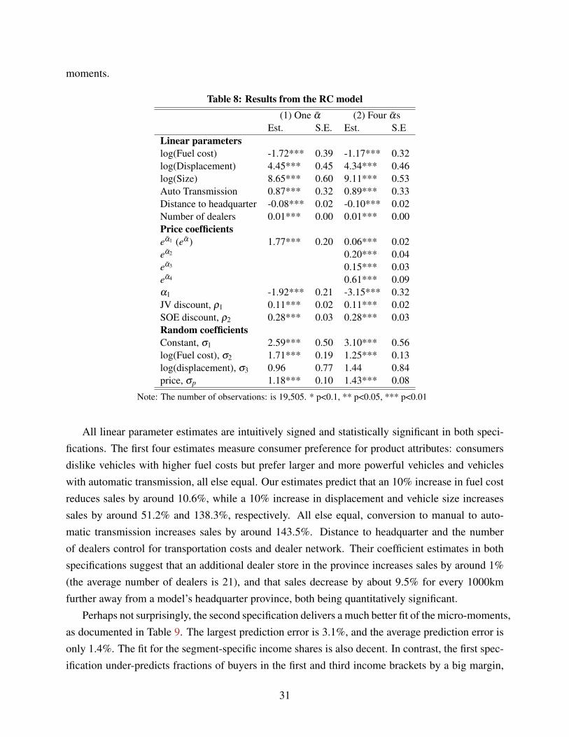
moments.

Table 8: Results from the RC model(1) One α (2) Four αs

Est. S.E. Est. S.ELinear parameterslog(Fuel cost) -1.72*** 0.39 -1.17*** 0.32log(Displacement) 4.45*** 0.45 4.34*** 0.46log(Size) 8.65*** 0.60 9.11*** 0.53Auto Transmission 0.87*** 0.32 0.89*** 0.33Distance to headquarter -0.08*** 0.02 -0.10*** 0.02Number of dealers 0.01*** 0.00 0.01*** 0.00Price coefficientseα1 (eα ) 1.77*** 0.20 0.06*** 0.02eα2 0.20*** 0.04eα3 0.15*** 0.03eα4 0.61*** 0.09α1 -1.92*** 0.21 -3.15*** 0.32JV discount, ρ1 0.11*** 0.02 0.11*** 0.02SOE discount, ρ2 0.28*** 0.03 0.28*** 0.03Random coefficientsConstant, σ1 2.59*** 0.50 3.10*** 0.56log(Fuel cost), σ2 1.71*** 0.19 1.25*** 0.13log(displacement), σ3 0.96 0.77 1.44 0.84price, σp 1.18*** 0.10 1.43*** 0.08

Note: The number of observations: is 19,505. * p<0.1, ** p<0.05, *** p<0.01

All linear parameter estimates are intuitively signed and statistically significant in both speci-fications. The first four estimates measure consumer preference for product attributes: consumersdislike vehicles with higher fuel costs but prefer larger and more powerful vehicles and vehicleswith automatic transmission, all else equal. Our estimates predict that an 10% increase in fuel costreduces sales by around 10.6%, while a 10% increase in displacement and vehicle size increasessales by around 51.2% and 138.3%, respectively. All else equal, conversion to manual to auto-matic transmission increases sales by around 143.5%. Distance to headquarter and the numberof dealers control for transportation costs and dealer network. Their coefficient estimates in bothspecifications suggest that an additional dealer store in the province increases sales by around 1%(the average number of dealers is 21), and that sales decrease by about 9.5% for every 1000kmfurther away from a model’s headquarter province, both being quantitatively significant.

Perhaps not surprisingly, the second specification delivers a much better fit of the micro-moments,as documented in Table 9. The largest prediction error is 3.1%, and the average prediction error isonly 1.4%. The fit for the segment-specific income shares is also decent. In contrast, the first spec-ification under-predicts fractions of buyers in the first and third income brackets by a big margin,

31

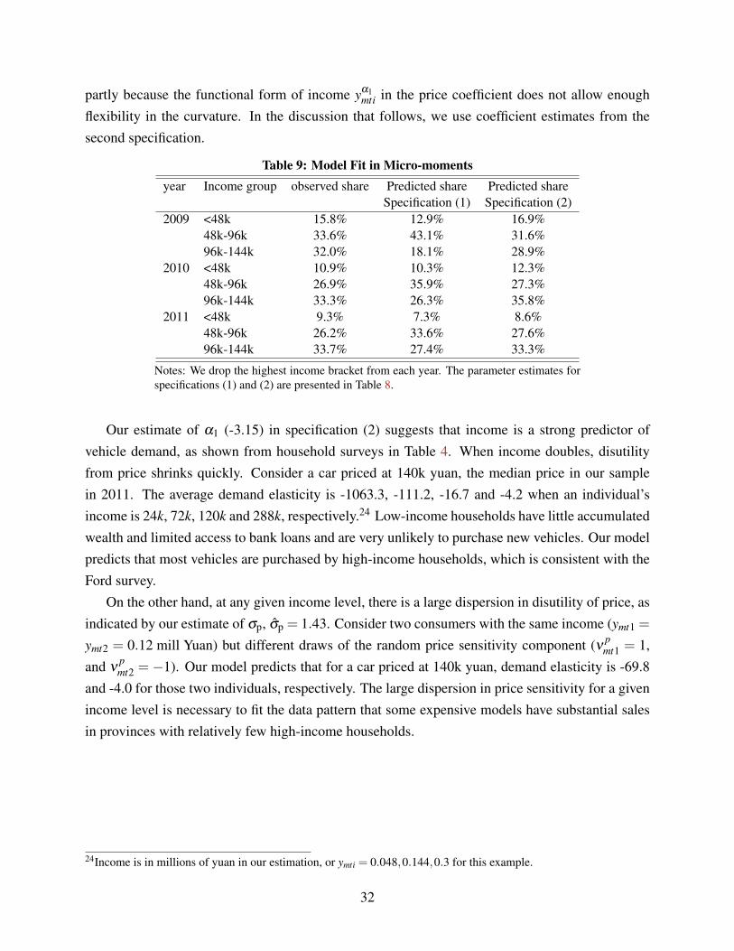
partly because the functional form of income yα1mti in the price coefficient does not allow enough

flexibility in the curvature. In the discussion that follows, we use coefficient estimates from thesecond specification.

Table 9: Model Fit in Micro-momentsyear Income group observed share Predicted share Predicted share

Specification (1) Specification (2)2009 <48k 15.8% 12.9% 16.9%

48k-96k 33.6% 43.1% 31.6%96k-144k 32.0% 18.1% 28.9%

2010 <48k 10.9% 10.3% 12.3%48k-96k 26.9% 35.9% 27.3%96k-144k 33.3% 26.3% 35.8%

2011 <48k 9.3% 7.3% 8.6%48k-96k 26.2% 33.6% 27.6%96k-144k 33.7% 27.4% 33.3%

Notes: We drop the highest income bracket from each year. The parameter estimates forspecifications (1) and (2) are presented in Table 8.

Our estimate of α1 (-3.15) in specification (2) suggests that income is a strong predictor ofvehicle demand, as shown from household surveys in Table 4. When income doubles, disutilityfrom price shrinks quickly. Consider a car priced at 140k yuan, the median price in our samplein 2011. The average demand elasticity is -1063.3, -111.2, -16.7 and -4.2 when an individual’sincome is 24k, 72k, 120k and 288k, respectively.24 Low-income households have little accumulatedwealth and limited access to bank loans and are very unlikely to purchase new vehicles. Our modelpredicts that most vehicles are purchased by high-income households, which is consistent with theFord survey.

On the other hand, at any given income level, there is a large dispersion in disutility of price, asindicated by our estimate of σp, σp = 1.43. Consider two consumers with the same income (ymt1 =

ymt2 = 0.12 mill Yuan) but different draws of the random price sensitivity component (ν pmt1 = 1,

and νpmt2 = −1). Our model predicts that for a car priced at 140k yuan, demand elasticity is -69.8

and -4.0 for those two individuals, respectively. The large dispersion in price sensitivity for a givenincome level is necessary to fit the data pattern that some expensive models have substantial salesin provinces with relatively few high-income households.

24Income is in millions of yuan in our estimation, or ymti = 0.048,0.144,0.3 for this example.

32

Figure 4: Price Elasticities and Markup-Price Ratios

To help understand the magnitude of the parameter estimates, we plot the 2011 own-price elas-ticities and Lerner index against vehicle price for each model in Figure 4. Own price elasticityvaries from -2.67 to -7.14, with a median of -4.88. Models with a higher price tend to have a lowerelasticity as shown in the top panel of Figure 4.25 The magnitudes of the own price elasticitiesare somewhat larger than those obtained for the U.S automobile market in Berry et al. (1995) andPetrin (2002). Chinese vehicle buyers have lower average income than those in U.S. and hence arelikely to be more price sensitive.26 The bottom panel of Figure 4 depicts the Lerner index using

25Everything else equal (for example, fixing individuals’ observed and unobserved preference), more expensive modelshave more elastic demand by construction. On the other hand, expensive models are typically purchased by wealthyindividuals who are less price sensitive, which is captured by the income variable in our price coefficient yα1

mti. How-ever, the income distribution we use is bounded above and capped at the maximum income observed in our 2005Census. For the ultra-expensive models that are priced above 600,000 RMB ($90,000), the upper bound of incomebecomes binding and the elasticity starts to increase after a certain point.

26As discussed in Section 2, brands produced by joint ventures and imports are one to three times more expansive inChina than in U.S..

33

before-tax prices. The ratio varies from 16.3% to 36.0%, with a mean of 22.2%. Products with ahigh price have a large Lerner index as buyers of those expensive automobiles tend to be less pricesensitive.

Estimates of ρ1 and ρ2 suggest that the price discount implied by local protectionism is equiva-lent to 11% of MSRP for local JV products and 28% for local SOE products. Some of the reporteddirect subsidies in Table 1 are as high as 15% of the auto price for local brands. Besides directreduction in the purchasing price, subsidies come in other forms including waivers of registrationfees and tolls and low-interest loans. There are also other implicit barriers to market access. Ourestimates of price discounts encapsulate the impact of all forms of local protectionism.

These very significant discounts, together with variation in products’ own-price elasticites, areconsistent with the magnitude of home bias for JV and SOE products estimated via the regressiondiscontinuity design in Table 5. For example, a 11% price discount for JVs and a price elasticity of-4.88 would imply roughly a 54% increase in sales, compared to 49% estimated in Table 5. In thebaseline specification, we normalize the price discount toward products by private automakers tozero based on the empirical evidence of no economically significant home bias for these products.In an alternative specification, we incorporate a separate price discount for local private products.The wedge between the coefficient of local private products and local JVs and SOEs remains thesame. If we interpret the (modest) coefficient of local private products as capturing the usual home-bias arising from preference (e.g., patriotism), then our results indicate that local protectionismappears much more important than local preference in affecting demand for local JV and SOEproducts.

5.2 Supply

Once we obtain demand parameters, we use the optimal pricing equation (8) to back out marginalcosts, taken into consideration the impact of the tax schedules and different ownership structuresacross firms. Here we assume Bertrand-Nash pricing with no collusion. We also estimate marginalcosts assuming that firms partially internalize interests of other firms with common ownership, asin Jie et al. (2013) and Miller and Weinberg (2016). For example, FAW-Toyota and Tianjin-Toyotashare a common foreign partner, which might soften the price competition between these firms.RESULTS TO BE ADDED.

To examine how car attributes and firm type affect marginal costs, we regress log of marginalcosts on these controls (see equation (9) for the marginal cost equation). There are 631 observationsin total, one for each model-year, since prices are set at the national level. Table 10 presentsresults for the base specification, with marginal cost being constant in quantity and assuming nocollusion. Column (1) includes the key attributes and their squared terms, and a separate dummy for

34

vehicle segment SUV and MPV. Column (2) adds brand fixed effects. Column (3) further includesestimated ˆξmt j from the demand-side to control for unobserved product quality. We average ˆξmt j

across provinces to obtain the national average. In Column (4) and (5), we break down JV productsby the origin of the foreign partner (Column (4)), and add a control for labor cost at the plantlocation (Column (5)).27

The coefficients on car attributes are in general intuitive. For example, marginal costs are higherfor larger engine size, larger cars, cars with auto transmission, and SUVs. Multi-purpose vehiclesegment includes a variety of specialized cars, including mini-buses that are often of lower qualitywith lower prices. Their marginal cost is lower than that for the other two segments. The onlyexception is the coefficient for fuel costs. The positive coefficient on fuel use implies that it ischeaper to produce more fuel efficient cars, which is somewhat puzzling. This might be driven bythe high correlation between fuel use, engine size, and size.

Turning to the relative cost efficiency among private, SOE, JV, and foreign auto makers, resultsfrom Column (1) suggest that private firms and SOEs enjoy 25% to 34% cost advantage over JVs(the base group) and a similar advantage over imports. This is mostly driven by different productmix between private/SOE and JV/foreign firms. Compared with domestic auto firms, JVs andforeign firms produce more high-end products (leather seats, sunroof, etc.) that are more likely touse high quality parts. Once we control for brand fixed effects (Column (2) onward), the gap inmarginal costs reduces by a large margin. Private firms are the most cost efficient among the fourgroups, and their marginal cost is about 5-6% lower than that of JVs across different specifications.Imports are the close runner-up, with a 4-5% of cost advantage.

Surprisingly, JVs do not seem to be more cost efficient than SOEs, even though all foreignpartners are well-known leading auto producers in the world. When we separate JVs by the coun-try origin of their foreign partners, we find that JVs with US, Japanese and Korea partners havesimilar cost efficiency to the SOEs. JVs with European partners appear the least efficient, and theirmarginal cost is 9% higher than that of domestic private auto firms.

The fact that JVs do not appear more efficient than SOEs might be related to how they aremanaged. First, every domestic partner of a JV is an SOE in our sample period.28 Second, theseSOE domestic partners hold at least 50% stake in a JV and in most cases control the operation andmanagement of the firm, while the foreign partner mainly provides the technology.

27Wages for automakers at the city level are difficult to find. Instead, we use each city’s median urban household incomedivided by the average household size from the 2005 Census as a proxy for auto-workers’ wage. For imports, we usethe maximum of our constructed city-level ‘wage’, since wages for auto-workers in Europe, U.S.A., or Japan/SouthKorea are much higher than those in China.

28The only private firm that formed a joint venture with foreign producers in our sample is Youngman Lotus, but ithad negligible sales and ceased passenger car production in 2015 and was dropped in our estimation. The first jointventure between a prominent private and a foreign auto producer happened in 2010, when BYD and Mercedes-Benzformed a joint venture BYD Daimler. Their first production debuted in 2014.

35

The medium marginal cost of a JV product in our sample is around 100k yuan. The transfer ofvehicle production from JVs to private firms would lead to a cost saving of about 6%, or around 6kyuan per vehicle.

Table 10: Results from cost-side estimations

(1) (2) (3) (4) (5)Est. S.E. Est. S.E Est. S.E Est. S.E Est. S.E

Private -0.08*** 0.03 -0.04*** 0.02 -0.04** 0.02 -0.04* 0.02 -0.04** 0.02JV/JV(US) 0.25*** 0.02 0.02 0.02 0.02 0.02 0.01 0.02 0.01 0.02JV(Japan) -0.00 0.02 -0.00 0.02JV(Korea) 0.03 0.02 0.03 0.02JV(Europe) 0.06*** 0.02 0.06** 0.02Imports 0.33*** 0.04 -0.02 0.03 -0.02 0.03 -0.02 0.02 -0.04 0.03Fuel use2 -0.01 0.00 -0.01** 0.00 -0.01** 0.00 -0.01** 0.00 -0.01** 0.00Engine size 1.38*** 0.16 0.71*** 0.11 0.67*** 0.10 0.71*** 0.10 0.70*** 0.10Engine size2 -0.17*** 0.03 -0.08*** 0.02 -0.07*** 0.02 -0.07*** 0.02 -0.07*** 0.02Size -0.33*** 0.11 0.07 0.07 0.15** 0.06 0.13** 0.06 0.13** 0.06Size2 0.03*** 0.01 0.00 0.00 -0.00 0.04 -0.00 0.00 -0.00 0.00Auto Trans. 0.18*** 0.02 0.12*** 0.01 0.12*** 0.01 0.12*** 0.01 0.12*** 0.01SUV 0.04 0.03 0.09*** 0.02 0.08*** 0.02 0.09*** 0.02 0.09*** 0.02MPV -0.06* 0.03 -0.05** 0.02 -0.05** 0.02 -0.04** 0.02 -0.04** 0.02ln(labor cost) 0.14 0.12year FE Y Y Y Y YBrand FE N Y Y Y Yξ N N Y Y Y

Note: The number of observations is 631. The reference firm type is JV in Columns (1) to (3), and JV(US) inColumns (4) and (5). Brand fixed effects and ξ are from the demand estimation. *p<0.1, ** p<0.05, *** p<0.01.

6 Simulations and Welfare Analysis

We examine what would happen in terms of market outcomes and social welfare if the trade barriersacross regions are eliminated. We conduct simulations based on 2011 to illustrate the results.

6.1 Impacts on Market Outcomes

We first predict vehicle sales setting the discount rates ρ1 and ρ2 to zero to mimic a world withoutlocal protectionism. The top panel of Table 11 demonstrates that SOE products would lose threequarters of the sales in their headquarter (home-market) province, while JV products lose about onethird of their home-market sales. In contrast, the impact of removing local protection on nationalvehicle sales is much smaller: in the absence of any price adjustment, the national market sharereduces by 4.1% for SOEs and 0.8% for JVs. Relative to free trade, local protection increases

36

SOEs’ and JVs’ national sales by a modest margin. This occurs for two reasons. First, there are31 provinces in China and each firm has only one home market. As a result, home-market sales,which directly benefit from local protection, only account for 5% of national vehicle sales for themedian vehicle. Second, when all provinces implement local protection, a SOE or JV auto-markerbenefits in its home province but loses in other provinces. This kind of business-stealing offsetsthe effectiveness of local protection in increasing national demand for locally protected products.In theory, higher local demand could be entirely offset by lower sales elsewhere, as in the classicexample of prisoners’ dilemma. In our setting, the local benefit on average outweighs the losseselsewhere, though there is considerable heterogeneity among different vehicle models.

When we remove local protection, a significant fraction of sales lost by these protected localproducts goes to similar non-local products, rather than the outside option. This kind of substitutionleads to a 3.0% increase in national sales of private brands, and a 0.8% increase for imported brands.Consumers who switch away from a local SOE or JV product tend to be more price sensitive andand are unlikely to substitute towards expensive imported products. Private brands benefits themost because their prices are on average lower than other products and they have similar attributesto the heavily protected SOE brands.

If price discounts were to be removed as a correction of existing policies, firms would adjustprices to cope with the loss of their home biass. The bottom panel of Table 11 reports changes insales when prices are allowed to change and Figure 5 plots the distribution of price updates by firmtypes.29 The magnitudes of the average price adjustments are small since removing local protectiononly has limited impacts on national vehicle demand. The majority of the JV and SOE productswould see price cuts due to significant demand loss in the home market.

The magnitude of the price adjustment is highly correlated with the importance of the homemarket. For example, the largest price reductions (-1.71% and -2.38%) come from two models pro-duced by Xiali, whose home-market sales account for around 20% of their national sales, relativeto the medium model whose home-market sales account for 5% of its national sales. In addition,products with a small home market may experience a gain in their national sales and report a priceincrease as a result.

29For each year, we numerically solve a system of J non-linear equations following the optimal pricing equation inpage 21. J is the number of models in that year.

37

Table 11: Impacts of Removing Local Protection on Sales in 2011Firm type Home-market Sales (’000) National Sales (’000)

Before After % Change Before After % Change

Without price updatesPrivate 74 76 2.6% 967 996 3.0%JV 426 294 -31.1% 6232 6184 -0.8%SOE 105 25 -76.4% 1277 1224 -4.1%Imports 357 360 0.8%

With price updatesPrivate 74 76 2.2% 967 988 2.1%JV 426 295 -30.7% 6232 6190 -0.7%SOE 105 26 -75.4% 1277 1244 -2.6%Imports 357 359 0.6%

Compared to SOE and JV products, the price adjustments for private and imported products aresmaller in absolute value, which is driven by two opposing forces. On one hand, the removal oflocal protectionism increases demand for these products, exerting upward pressure on prices. Onthe other hand, prices are strategic substitutes. When SOEs and JVs reduce their prices, it exertsdownward pressure on prices of private and imported cars. Note that in our setting with multi-product firms and price discounts that are local in nature, patterns of price adjustments are morecomplex than that of a single-product firm in a national market.

Figure 5: Percentage Price Changes by Firm Type

Overall, the removal of local protectionism leads to a price reduction for the majority of the

38

products while the decreases are larger for JV and SOE products than for products from privateand foreign automakers. As shown in the bottom panel of Table 11, these price changes help tocounteract part of the reduction in sales when local protection is absent.

6.2 Welfare Analysis

We now examine the welfare consequences of local protectionism separately for consumer surplus,firm profits, and tax revenue. The removal of local protection increases consumer welfare throughtwo channels. First, the simulations above demonstrate that the majority of the vehicle modelswould see price cuts absent local protectionism. Second, local protection distorts consumer choicestoward SOE or JV products that can be suboptimal. Eliminating local protection gets rid of suchchoice distortions and increases welfare.

To illustrate the welfare loss of choice distortions, consider a simple example where consumeri in market m obtains a consumer surplus of 10,000 yuan from her top choice product A, and asurplus of 6000 yuan from a local product B. Suppose that the government in market m providesa subsidy of 5000 yuan to consumers who purchase B. The subsidy leads consumer i to choose Bover A, which entails a welfare loss of 4000 yuan: the government spends 5000 yuan subsidingconsumer i’s vehicle purchase, but only increases her surplus by 1000 yuan. We incur such losseswhenever local protection causes a consumer to choose a suboptimal local brand that is differentfrom her intrinsic top choice. Importantly, the magnitude of the welfare loss is solely determinedby the gap in the intrinsic utility between a consumer’s top choice and the subsidized product, andis independent of the size of subsidy.

To compare consumer surplus with and without subsidies, we use simulations. For each province,we draw 1,000 pseudo consumers using the empirical income distribution and 20,000 random εi

vectors for each consumer. Then we calculate the monetized difference in the intrinsic utility be-tween a consumer’s top choice without protection and with protection. The intrinsic utility of thetop choice without protection is:

Max Utility = maxj=0,...,J

{u1i jm + εi jm} (10)

where u1i jm is the same as that defined in equation (3) but excludes the price discounts for local JVs

and SOEs. The intrinsic utility of the best choice under protection is:

Max UtilityProtection = maxj=0,...,J

{ui jm + εi jm}−ρkmt p0kmt |k=argmax j=0,...,J{ui jm+εi jm} (11)

where ui jm is the same as that defined in equation (3), k is the top choice under local protection,and ρkmt p0

kmt is the subsidy (price discount) associated with choice k. The difference between

39

(10) and (11), averaged across εi draws and divided by αmti (consumer i’s price sensitivity), is thewelfare loss associated with choice distortions for consumer i. We average the welfare loss acrossconsumers and multiply it with the market size to obtain the total welfare loss in market m underlocal protection. Then we aggregate it to the national level to obtain the welfare gain from removinglocal protection nationwide.

Note that not all local protection is equated as monetary price discounts. One might be con-cerned that this could overstate the loss of protection since local protection comes in many forms,and not all of them involve monetary subsidy. Fortunately, whether local protection involves mone-tary subsidy is irrelevant for the calculation here, since the magnitude of the welfare loss of choicedistortions only depends on the gap of the intrinsic utility between a consumer’s top choice and thesubsidized product.

Figure 6: Consumer welfare gains through removing local protection (bn. yuan), 2011

0

0.1

0.2

0.3

0.4

0.5

0.6

0.7

0.8

Original price Revised Price

Figure 6 shows predicted consumer welfare gains in 2011 by provinces when choice distortionis eliminated. The blue bars show welfare gains from choice elimination only, while the orangebars include additional welfare gains after firms update their prices.30 As expected, welfare gainis higher in larger markets such as Guangdong, and in provinces that house more native JV andespecially SOE brands. For example, Anhui only account for 2.9% of total vehicle sales in Chinain 2011, ranked 13 out of the 31 provinces. However, it records the second highest expected welfaregains since it is the home to two of the largest SOE brands, Chery and JAC.

Our simulations show that consumer welfare gain from the elimination of choice distortions is2.5 billion yuan, or roughly 22% of total subsidies in 2011. Allowing prices to adjust further leadsto an additional welfare gain of one billion yuan. Over the three-year period, total expected welfare30The graph only shows 14 provinces that have at least one native JV or SOE brands. The other 17 provinces mainly

benefit from price reductions.

40

gain from the elimination of local protection is 12.3 billion yuan (nearly $2 billion), or 36.7% oftotal subsidies for local products.

While local protectionism reduces consumer welfare shown above, Table 12 presents its impacton firm profit and tax revenue. Removing local protection reduces the profits of, and the tax rev-enue from, JVs and SOEs while benefits private automakers and imports. The elimination of thesubsidies to local JVs and SOEs would lead some consumers to switch to products from privateand foreign automakers, as well as the outside good. The simulation results illustrate that the re-moval of local protection would lead to a reduction of 2.9 and 2.6 billion yuan in firm profit andtax revenue in 2011, respectively.

Table 12: Impacts of Removing Local Protection on Profits and Tax in 2011Firm type Total Profit (bill.) Tax Revenue (bill.)

Before After % Change Before After % ChangeWithout price updatesPrivate 10.3 10.6 2.8% 17.2 17.7 2.7%JV 223.5 221.7 -0.8% 297.9 295.3 -0.8%SOE 17.4 16.8 -3.5% 27.1 26.1 -3.6%Imports 27.6 27.8 0.8% 62.2 62.7 0.7%

With price updatesPrivate 10.3 10.5 2.0% 17.2 17.6 2.0%JV 223.5 221.1 -1.1% 297.9 295.6 -0.8%SOE 17.4 16.7 -4.0% 27.1 26.2 -3.2%Imports 27.6 27.7 0.5% 62.2 62.6 0.5%

Notes: The unit for profit and tax revenue is billion yuan.

Figure 7 shows the impact of removing local protection on firm profit for selected firms of dif-ferent ownership type (the first four are private automakers; the next six are SOEs; the six after thatare JVs; and the last two are imports). Consistent with the table above, local protection generallybenefits JVs and SOEs at the expense of private automakers and imports. Nevertheless, there issome heterogeneity across firms even within the same ownership type. Among SOEs, Brillanceand Xiali enjoy a very large benefit from local protection while Haima suffers from local protectivepolicies. This heterogeneity is driven by the fact that local protection is a double-edged sword inthat it benefits the firm in the local market but it hurts the firm in non-local markets. If the productis unpopular in the local market31(such is the case for BMW-Brilliance) or the local market is toosmall (such is the case for Haima) for example due to poor compatibility with the local marketdemographics, the net impact of the local protection could be negative. On the other hand, Bril-

31One reason for this to happen is that a product may be a poor match for the population demographics in its homemarket. For example, BMW-Brilliance sells high-end products that are unaffordable for most consumers in its homemarket Liaoning.

41

liance and Xiali are very popular brand in the local market but fairs poorly in non-local market (forexample due to poor reputation in the those markets). Local protection can benefit these brandslocally much more than it hurts them in non-local markets.

Figure 7: Impact on Firm Profit by Firm Type

‐12%

‐10%

‐8%

‐6%

‐4%

‐2%

0%

2%

4%

A significant portion of the profit and tax revenue loss arises from consumers switching awayfrom the once-protected local brands to the outside option. One needs to be careful in interpretingthese loss as net ‘welfare loss’, as it is more appropriate to view them as a redistribution acrossdifferent industries. Our supply side is a partial analysis and does not model the profit and taxrevenue associated with the outside good (or the spending on other types of goods). When con-sumers switch to the outside option, they are likely to spend on public transportation, used cars, orother economic activities that would generate profits and tax revenue elsewhere. While the reduc-tion of local car production would indeed hurt the auto industry (or more specifically, most JV andSOE automakers), its economy-wide impact on industry profits and tax revenues is ambiguous andbeyond the scope of our analysis.

The tangible part of welfare impact on the firm side is driven by substitution across products.For example, the removal of local protection could lead to larger sales of more or less profitableproducts. To examine this, we use numeric simulations to separate substitutions among differentcar products from substitutions to the outside option.32 Our results show that in 2011 JVs and SOEswould lose 33,542 and 20,157 units of sales to the outside option, corresponding to a net profit lossof 1.1 billion and a tax revenue loss of 1.6 billion. The remainder of 1.8 and 1.0 billion in profit32For every pseudo household in each market with a native JV or SOE brand, we draw 20,000 vectors of εi, each of

which pins down household i’s top choice with and without local protection. We then average the substitution patternsover 20,000 draws to obtain substitution patterns by household i, and average over the 1000 pseudo households toreplicate substitution patterns in each market.

42

and revenue loss comes from substitutions across products in two ways. First, JVs and SOEs lose20,298 units to private product and 2271 units to imports.33. Private firms typically have chargelower prices, thinner profit margins, and pay lower taxes. The medium profit margin is around 10k,25k, 11k, 73k per vehicle for private, JV, SOE, and imported brands, respectively. Second, majorityof the substitutions happen between products under the same type of firm. In 2011, JVs and SOElose 94,266 and 39,035 units of sales each to other JVs and SOEs. When consumers switch awayfrom a local product after the removal of subsidies, they are more likely to choose cheaper productsthat fetch lower profit margin and pay less tax. During the three-year period, total profit and taxrevenue loss from substitution across products is 4.9 billion yuan and 3.1 billion yuan, respectively.

So far we have ignored the fact that tax collection is necessary to finance government subsidiesand that the marginal excess burden per additional dollar of tax revenue is non-trivial. Accordingto Ballard et al. (1985), the welfare loss from a 1 percent increase in all distortionary tax rates isin the range of 17 to 56 cents per dollar of extra revenue in the U.S., using elasticity assumptionsthat appear plausible. There are many reasons to believe that the marginal excess burden for taxcollection is higher in China, since taxed activities are likely to be more elastic, market distortionsare more severe, and tax evasion is prevalent. The total amount of tax subsidy is estimated to be34 billion Yuan during our sample period. Assuming the marginal excess burden is 37 cents perYuan (37%) using the mid point of the estimates provided by Ballard et al. (1985), the welfare lossassociated with the tax collection to finance subsidies amounts to 12.58 billion Yuan. Even if theactual monetary subsidy is half of our estimates (which captures implicit barriers in addition todirect subsidies), the welfare loss associated with tax collection is still substantial.

Overall, our results suggest that the removal of local protection would induce more intenseprice competition and improve consumer surplus by 12.3 billion yuan through eliminating choicedistortions. At the same time, it would lead to a total loss of 8.0 billion yuan in profits and taxrevenues as sales accrue to less profitable firms. Our cost-side estimates suggest that private firmsare more cost-efficient than SOEs and JVs by around 5%. While the magnitude of such cost-savings is small in the short-run, eliminating local protection would benefit the growth of privatefirms, which in turn would lead to a more competitive landscape of the auto industry in the longrun that benefits consumers and leads to more efficient allocation of production.

33Consumers who switch away from an once-protected local product are much more likely to choose private productsthan imports for three main reasons. First, private products start with a larger market share than imports. Second,private products are much closer substitutes to the heavily protected SOE products as well as most JV productscompared to the imports, as shown in Table 3. Third, consumers who change their minds due to a price discount aretypically sensitive to prices and unlikely to purchase expensive imports. As can be seen from Figure 7, private firmsstand to gain much more from the abolition of local protection compared to the foreign firms.

43

7 Conclusion

Based on the census of new passenger vehicle registrations from 2009 to 2011 in China, we providerobust evidence of local protectionism in China’s automobile market using a regression discontinu-ity design. Through a structural model of vehicle demand and supply, we then quantify the impactsof local protectionism on market outcomes and show that abolishing local protection would signif-icantly improve consumer welfare at the expense of a smaller loss of firm profits and tax revenues.In addition, the shift of production from high-cost SOEs to low-cost private firms would makeresource allocations more efficient across firms and foster productivity growth. Our findings there-fore call for close attention of central policy makers on eradicating trade barriers across regions andfacilitating market integration within the country as China tries to spawn the next wave of economicgrowth.

While our study is the first to examine the impacts of local protectionism on market outcomesand social welfare focusing on an output market in China, future research could explore its long-term impacts on market structure such as firm entry and exit, innovation and productivity. Thiswould help us understand the extent to which local protectionism has led to the salient featuresobserved in this industry such as a large number of automakers, production capacity being scatteredaround the country, and low capacity utilization. In addition, it would be interesting to furtherexplore the incentives of local governments and understand the balances they are trying to strikebetween consumer welfare, GDP growth, and tax revenue.

44

References

Anderson, James, Catherine Milot, and Yoto Yotov, “How Much Does Geography Deflect Ser-vices Trade? Canadian Answers,” International Economic Review, 2014, 55, 791–818.

Atkin, David and Dave Donaldson, “Who’s Getting Globalized? The Size and Nature of Interna-tional Trade Costs,” 2016. Working Paper.

Bai, Chong-En, Yingjuan Du, Zhigang Tao, and Yueting Sarah Tong, “Local Protectionismand Regional Specialization: Evidence from China’s Industries,” Journal of International Eco-

nomics, 2004, 63, 397–417.

Baily, Martin, Charles Hulten, and David Campbell, “Productivity Dynamics in ManufacturingPlants,” Brooking Papers on Economic Activity: Microeconomics, 1992, pp. 187–267.

Ballard, Charles L., John B. Shoven, and John Whalley, “General Equilibrium Computationsof the Marginal Welfare Costs of Taxes in the United States,” The American Economic Review,1985, 75.

Banerjee, Abhijit and Kaivan Munshi, “How Efficiently is Capital Allocated? Evidence fromthe Knitted Garment Industry in Tipur,” Review of Economic Studies, 2004, 71, 19–42.

Berry, Steven, “Estimating Discrete Choice Models of Product Differentiation,” RAND Journal of

Economics, 1994, 25 (2), 242–262.

, James Levinsohn, and Ariel Pakes, “Automobile Prices in Market Equilibrium,” Economet-

rica, 1995, 63 (4), 841–890.

Brandt, Loren, Trevor Tombe, and Xiaodong Zhu, “Factor market distortions across time, spaceand sectors in China,” Review of Economic Dynamics, 2009, 16, 39–58.

Bronnenberg, Bart J., Jean-Pierre H. Dub, and Matthew Gentzkow, “The Evolution of BrandPreferences: Evidence from Consumer Migration,” American Economic Review, 2012, 102,2472–2508.

Canli, Zeynep Gurhan and Durairaj Maheswaran, “Determinants of Country-of-Origin Evalu-ations,” Journal of Consumer Research, 2000, 27 (1), 96–108.

Cosar, A. Kerem and Pablo D. Fajgelbaum, “Internal Geography, International Trade, and Re-gional Specialization,” American Economic Journal: Microeconomics, 2016, 8, 24–56.

, Paul L. Grieco, Shengyu Li, and Felix Tintelnot, “What Drives Home Market Advantage?,”2016. Working Paper.

Faber, Benjamin, “Trade integration, market size, and industrialization: Evidence from china’s

45

national trunk highway system,” The Review of Economic Studies, 2014, 81:3, 1046–1070.

Fajgelbaum, Pablo D., Eduardo Morales, Juan Carlos Suez Serrato, and Owen Zidar, “StateTaxes and Spatial Misallocation,” 2016. Working Paper.

French, Kenneth and James Poterba, “Investor Diversification and International Equity Mar-kets,” American Economic Review, 1991, 81.

Goldberg, Pinelope and Frank Verboven, “Evolution of Price Dispersion in the European CarMarket,” Review of Economic Studies, 2011, 68, 811–848.

Holmes, Thomas J., Ellen R. McGrattan, and Edward C. Prescott, “Quid Pro Quo: TechnologyCapital Transfers for Market Access in China*,” The Review of Economic Studies, 2015.

Holz, Carsten, “No Razor?s Edge: Reexamining Alwyn Young?s Evidence for In- creasing Inter-provincial Trade Barriers in China,” Review of Economics and Statistics, 2009, 91, 599–616.

Hsieh, Chang-Tai and Peter J. Klenow, “Misallocation and Manufacturing TFP in China andIndia,” Quarterly Journal of Economics, 2009, 124, 1403–1488.

Hu, Weimin, Junji Xiao, and Xiaolan Zhou, “Collusion or Competition? Inter-firm Relationshipsin the Chinese Auto Industry,” Journal of Industrial Economics, 2014, LXII, 1–40.

Jin, Hehui, Yingyi Qian, and Barry R. Weingast, “Regional Decentralization and Fiscal Incen-tives: Federalism, Chinese Style,” Journal of Public Economics, 2005, 89, 1719–1742.

Klein, Jill and Richard Ettensoe, “Consumer Animosity and Consumer Ethnocentrism: An Anal-ysis of Unique Antecedents,” Journal of International Consumer Marketing, 1999, 11 (4), 5–24.

Li, Shanjun, Junji Xiao, and Yiming Liu, “The Price Evolution in China’s Automobile Market,”Journal of Economic Management and Strategy, 2015.

, Lang Tong, Jianwei Xing, and Yiyi Zhou, “The Market for Electric Vehicles: Indirect Net-work Effects and Policy Impacts,” Journal of the Association of Environmental and Resource

Economists, 2016.

McCallum, John, “National Borders Matter: Canada-U.S. Regional Trade Patterns,” American

Economic Review, 1995, 85.

Miller, Nathan and Matthew Weinberg, “The Market Power Effects of a Merger: Evidence fromthe U.S. Brewing Industry,” 2016. working paper.

Oats, Wallace, Fiscal Federalism, New York: Harcourt Brace Jovanovich, 1972.

Peek, Joe and Eric Rosengren, “Unnatural Selection: Perverse Incentives and the Misallocationof Credit in Japan,” American Economic Review, 2005, 95, 1144–1166.

46

Petrin, Amil, “Quantifying the benefit of new products: the case of minivan,” Journal of Political

Economy, 2002, 110 (4), 705–729.

Restuccia, Diego and Richard Rogerson, “Policy distortions and aggregate productivity withheterogeneous establishments,” Journal of Development Economics, 2008, 11, 707–720.

Schmalensee, R., “Product Differentiation Advantages of Pioneering Brands,” American Eco-

nomic Review, June 1982, 72 (3), 349–365.

Shimp, Terence A. and Subhash Sharma, “Consumer Ethnocentrism: Construction and Valida-tion of the CETSCALE,” Journal of Marketing Research, 1987, 24.

Sutton, John, Sunk Costs and Market Structure: Price Competition, Advertising, and the Evolution

of Concentration, MIT Press, 1991.

Young, Alwyn, “The Razor?s Edge: Distortions and Incremental Reform in the People?s Republicof China,” Quarterly Journal of Economics, 2000, 115, 1091–1135.

Yu, Rose, Colum Murphy, and Mike Ramsey, “Subsidies Stoke China’s Domestic Car Makers,”The Wall Street Journal, May 2014.

47

AppendicesA home bias by Firm

The table below shows the market share in sales by firm at the national level and in the homemarket (where the firm is headquartered). The last column is the percentage difference in the shareof dealers at the national level and in the home market. Most private firms do not fare much betterin their home markets; every single SOE has very stark advantage in its home market; JVs liesomewhere in-between. The differences in dealer counts are typically below those in sales.

Table 1: home bias by Firm

Firm National Home % Difference % Difference inShare Share in Sales Dealers %

Private FirmsBYD 4.70% 4.93% 5% 15%Geely 3.73% 2.10% -44% -22%Great Wall 2.04% 3.33% 63% 3%Lifan 0.38% 0.99% 161% 91%Zotye 0.30% 0.25% -17% -37%SOEsChery 4.70% 11.70% 149% 72%FAW 2.41% 7.27% 202% 177%Xiali 2.36% 16.40% 595% 341%Chana 1.52% 4.60% 203% 181%JAC 1.32% 5.49% 316% 139%Haima 1.30% 2.67% 105% 77%Brilliance 0.87% 3.07% 253% 222%JVsVW Shanghai 9.98% 28.16% 182% 85%GM Shanghai 9.98% 18.06% 81% 68%VW FAW 7.90% 21.57% 173% 51%Hyundai Beijing 6.55% 7.50% 14% 8%Nissan Dongfeng 5.69% 11.43% 101% 41%Toyota FAW 4.95% 4.30% -13% 3%Ford Changan 3.97% 6.82% 72% 70%Honda Guangzhou 3.76% 7.11% 89% 79%PSA Dongfeng 3.37% 11.27% 234% 78%Kia Yueda 3.29% 3.31% 1% 21%Honda Dongfeng 2.55% 4.90% 93% 27%Toyota Guangzhou 2.48% 5.46% 120% 55%Suzuki Changan 1.91% 2.25% 18% -5%GM Shanghai Wuling 0.83% 3.70% 343% 197%Suzuki Changhe 0.82% 1.36% 66% 138%BMW Brilliance 0.64% 0.57% 11% 23%

1

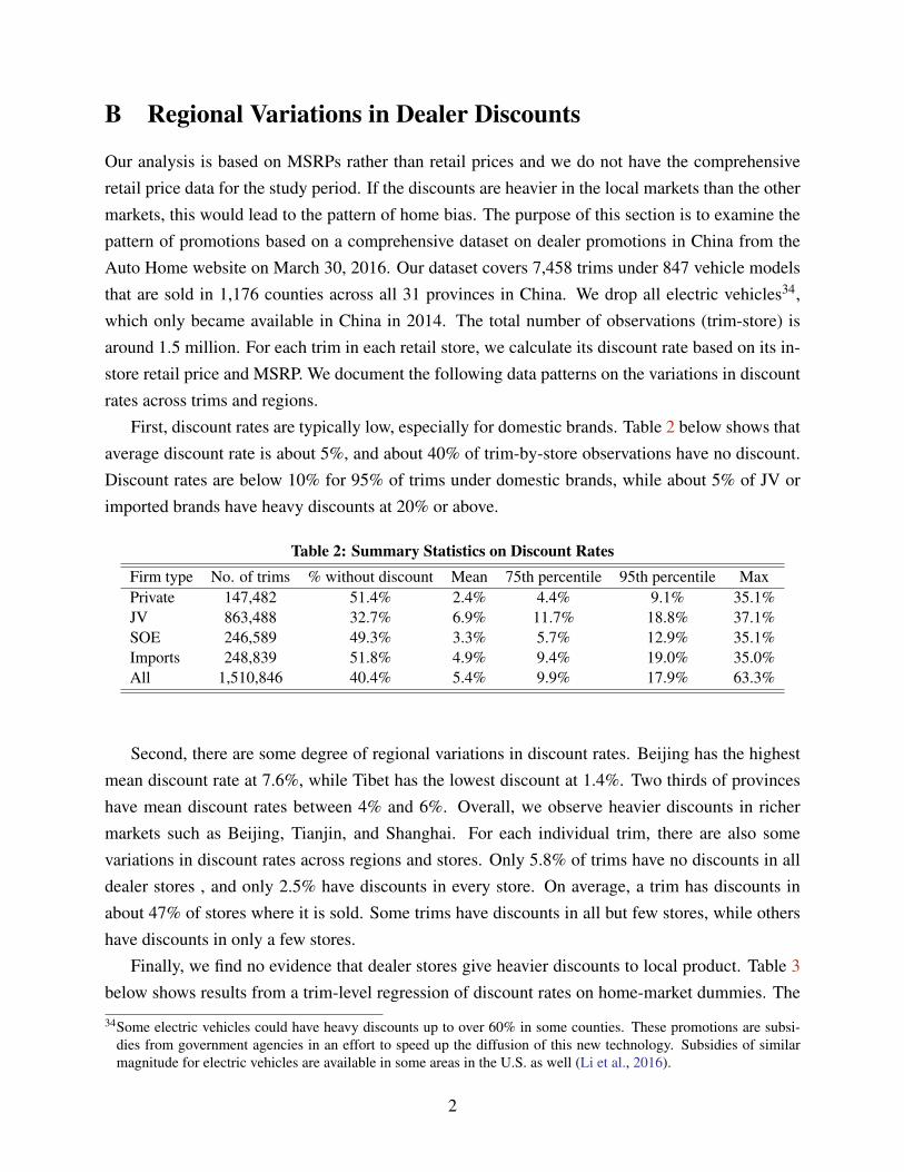
B Regional Variations in Dealer Discounts

Our analysis is based on MSRPs rather than retail prices and we do not have the comprehensiveretail price data for the study period. If the discounts are heavier in the local markets than the othermarkets, this would lead to the pattern of home bias. The purpose of this section is to examine thepattern of promotions based on a comprehensive dataset on dealer promotions in China from theAuto Home website on March 30, 2016. Our dataset covers 7,458 trims under 847 vehicle modelsthat are sold in 1,176 counties across all 31 provinces in China. We drop all electric vehicles34,which only became available in China in 2014. The total number of observations (trim-store) isaround 1.5 million. For each trim in each retail store, we calculate its discount rate based on its in-store retail price and MSRP. We document the following data patterns on the variations in discountrates across trims and regions.

First, discount rates are typically low, especially for domestic brands. Table 2 below shows thataverage discount rate is about 5%, and about 40% of trim-by-store observations have no discount.Discount rates are below 10% for 95% of trims under domestic brands, while about 5% of JV orimported brands have heavy discounts at 20% or above.

Table 2: Summary Statistics on Discount RatesFirm type No. of trims % without discount Mean 75th percentile 95th percentile MaxPrivate 147,482 51.4% 2.4% 4.4% 9.1% 35.1%JV 863,488 32.7% 6.9% 11.7% 18.8% 37.1%SOE 246,589 49.3% 3.3% 5.7% 12.9% 35.1%Imports 248,839 51.8% 4.9% 9.4% 19.0% 35.0%All 1,510,846 40.4% 5.4% 9.9% 17.9% 63.3%

Second, there are some degree of regional variations in discount rates. Beijing has the highestmean discount rate at 7.6%, while Tibet has the lowest discount at 1.4%. Two thirds of provinceshave mean discount rates between 4% and 6%. Overall, we observe heavier discounts in richermarkets such as Beijing, Tianjin, and Shanghai. For each individual trim, there are also somevariations in discount rates across regions and stores. Only 5.8% of trims have no discounts in alldealer stores , and only 2.5% have discounts in every store. On average, a trim has discounts inabout 47% of stores where it is sold. Some trims have discounts in all but few stores, while othershave discounts in only a few stores.

Finally, we find no evidence that dealer stores give heavier discounts to local product. Table 3below shows results from a trim-level regression of discount rates on home-market dummies. The

34Some electric vehicles could have heavy discounts up to over 60% in some counties. These promotions are subsi-dies from government agencies in an effort to speed up the diffusion of this new technology. Subsidies of similarmagnitude for electric vehicles are available in some areas in the U.S. as well (Li et al., 2016).

2

coefficients are small in magnitude, reflecting the low discount rates on average. After controllingfor province and trim fixed effects, the discount rate for private automakers and SOEs are nega-tive, implying that the discounts are even smaller in the local markets than in the other markets.Nevertheless, all three coefficients are small in magnitude and suggest no economically significantdifferences in discount rates between the local market and the other markets.

Table 3: Regional Variation in Promotions(1) (2) (3)

Est. S.E. Est. S.E. Est. S.E.HQ*Private -3.39*** 0.06 -0.18*** 0.05 -0.41*** 0.05HQ*SOE -2.31*** 0.05 0.04 0.04 -0.16*** 0.04HQ*JV 1.66*** 0.03 0.37*** 0.02 -0.03 0.02Trim FE N Y YProvince FE N N Y

Note: The number of observations is 1,510,846. The dependent variable is thediscount rate (in percentage points). * p<0.1, ** p<0.05, *** p<0.01.

C Logit Regressions

Our structural analysis incorporates local protection as price discounts for consumer purchase oflocal brands. Alternatively, we could capture local protection directly in the utility function as in thespatial discontinuity analysis in Section 3.2. In particular, we can specify the Berry-logit equationas the following:

ln(s jmt

s0mt) = β1LCL jm +β2LCL jmSOE j +β3LCL jmJV j

−αPj +X jθ + τB j +δm +ηt +ξ jmt ,

where j denotes a product (vehicle model), m province, and t year. LCL is a dummy for localproducts. There are two types of local products based on if product j is produced by an automakerheadquartered in market m or if it is produced by an automaker with a plant in market m. We allowthese two types of local products to have different levels of home bias. P j is the price of product j

while X j includes other observed vehicle attributes. B j, δm, ηt are brand (e.g., Toyota), province,and year fixed effects, respectively. To deal with the price endogeneity due to unobserved vehicleattributes, we use the same set of IVs as discussed in section 4.3 in Columns (2) to (4).

We conduct regressions separately for individual and institution purchases at the provincial-year-product level as in our structural analysis. Table 4 below presents the results from Berry-logitregressions for individual purchases. We find that JV and especially SOEs have large and statisti-cally significant home-market advantage in their headquarter provinces but private automakers donot. This is consistent with our results from the spatial discontinuity analysis in Section 3.2 and in-

3

forms our choice of allowing two free parameters for local discount rates in our structural analysis.The coefficient for Plant*SOE is statistically significant in the IV specifications, suggesting thatproducts from SOEs also enjoy an advantage in provinces where the automaker has manufacturingplants, although the magnitude is much smaller than the coefficient on HQ*SOE. The results alsoshow that controlling for dealer network and product-market distance only erode a small part ofhome-market advantages for local JVs and SOEs, as suggested from the spatial discontinuity anal-ysis. The results for institutional purchases presented in Table 5 show an even stronger home biasfor JVs and SOEs as local governments often require and encourage the purchase of local productsby government agencies and taxi companies for their vehicle fleet.

Table 4: Results from Berry-Logit Regressions, individual purchaseOLS IV I IV II IV III(1) (2) (3) (4)

HQ*Private 0.02 0.02 -0.10 0.04(0.11) (0.18) (0.16) (0.15)

HQ*JV 0.65*** 0.94*** 0.81*** 0.66***(0.06) (0.06) (0.07) (0.06)

HQ*SOE 1.32*** 1.59*** 1.46*** 1.32***(0.10) (0.09) (0.10) (0.10)

Plant*Private 0.01 -0.05 0.02 0.02(0.09) (0.12) (0.13) (0.13)

Plant*JV -0.07 0.23*** 0.20*** -0.07(0.07) (0.06) (0.06) (0.06)

Plant*SOE 0.45** 0.29 0.33* 0.45***(0.22) (0.19) (0.19) (0.18)

ln(Price) -0.41*** -3.07*** -3.07*** -3.03***(0.06) (0.18) (0.18) (0.18)

Distance -0.06*** -0.06*** -0.05***(0.01) (0.01) (0.01)

No. of Dealers 0.01*** 0.01***(0.00) (0.00)

Notes: The number of observations is 19,505 with the unit of obser-vation being province-year-product. All the regressions control forvehicle attributes, year and brand fixed effects, as well as market-specific preference for each vehicle type. p<0.1, ** p<0.05, ***p<0.01.

4

Table 5: Results from Berry-Logit Regressions, Institutional purchaseOLS IV I IV II IV III(1) (2) (3) (4)

HQ*Private 0.02 0.02 -0.10 0.04(0.11) (0.18) (0.16) (0.15)

HQ*JV 0.65*** 0.94*** 0.81*** 0.66***(0.06) (0.06) (0.07) (0.06)

HQ*SOE 1.32*** 1.59*** 1.46*** 1.32***(0.10) (0.09) (0.10) (0.10)

Plant*Private 0.01 -0.05 0.02 0.02(0.09) (0.12) (0.13) (0.13)

Plant*JV -0.07 0.23*** 0.20*** -0.07(0.07) (0.06) (0.06) (0.06)

Plant*SOE 0.45** 0.29 0.33* 0.45***(0.22) (0.19) (0.19) (0.18)

ln(Price) -0.41*** -3.07*** -3.07*** -3.03***(0.06) (0.18) (0.18) (0.18)

Distance -0.06*** -0.06*** -0.05***(0.01) (0.01) (0.01)

No. of Dealers 0.01*** 0.01***(0.00) (0.00)

Notes: The number of observations is 19,505 with the unit of obser-vation being province-year-product. All the regressions control forvehicle attributes, year and brand fixed effects, as well as market-specific preference for each vehicle type. p<0.1, ** p<0.05, ***p<0.01.

5