Local Model Checking of Weighted CTLwith Upper-Bound Constraints

Jonas Finnemann Jensen, Kim Guldstrand Larsen,Jirı Srba, and Lars Kaerlund Oestergaard

Department of Computer Science, Aalborg UniversitySelma Lagerlofs Vej 300, 9220 Aalborg, Denmark

jopsen@gmail.com, {kgl,srba}@cs.aau.dk, larsko@gmail.com

Abstract. We present a symbolic extension of dependency graphs byLiu and Smolka in order to model-check weighted Kripke structuresagainst the logic CTL with upper-bound weight constraints. Our ex-tension introduces a new type of edges into dependency graphs and liftsthe computation of fixed-points from boolean domain to nonnegativeintegers in order to cope with the weights. We present both global andlocal algorithms for the fixed-point computation on symbolic dependencygraphs and argue for the advantages of our approach compared to thedirect encoding of the model checking problem into dependency graphs.We implement all algorithms in a publicly available tool prototype andevaluate them on several experiments. The principal conclusion is thatour local algorithm is the most efficient one with an order of magni-tude improvement for model checking problems with a high number of“witnesses”.

1 Introduction

Model-driven development is finding its way into industrial practice within thearea of embedded systems. Here a key challenge is how to handle the growingcomplexity of systems, while meeting requirements on correctness, predictabil-ity, performance and not least time- and cost-to-market. In this respect model-driven development is seen as a valuable and promising approach, as it allowsearly design-space exploration and verification and may be used as the basis forsystematic and unambiguous testing of a final product. However, for embeddedsystems, verification should not only address functional properties but also anumber of non-functional properties related to timing and resource constraints.

Within the area of model checking a number of state-machine based modelingformalisms has emerged, allowing for such quantitative aspects to be expressed.In particular, timed automata (TA) [1], and the extensions to weighted timedautomata (WTA) [6,2] are popular and tool-supported formalisms that allow forsuch constraints to be modeled.

Interesting behavioural properties of TAs and WTAs may be expressed innatural weight-extended versions of classical temporal logics such as CTL for

branching-time and LTL for linear-time. Just as TCTL and MTL provide ex-tensions of CTL and LTL with time-constrained modalities, WCTL and WMTLare extensions with weight-constrained modalities interpreted with respect toWTAs. Unfortunately, the addition of weight now turns out to come with aprice: whereas the model-checking problems for TAs with respect to TCTL andMTL are decidable, it has been shown that model-checking WTAs with respectto WCTL is undecidable [9].

In this paper we reconsider this model checking problem in the setting ofuntimed models, i.e. essentially weighted Kripke structures, and negation-freeWCTL formula with only upper bound constraints on weights. As main contri-butions, we show that in this setting the model-checking problem is in PTIME,and we provide an efficient symbolic, local (on-the-fly) model checking algorithm.

Our results are based on a novel symbolic extension of the dependency graphframework of Liu and Smolka [16] where they encode boolean equation systemsand offer global and local algorithms for computing minimal and maximal fixedpoints in linear time. Whereas a direct encoding of our model checking prob-lem into dependency graphs leads to a pseudo-polynomial algorithm1, the novelsymbolic dependency graphs allow for a polynomial encoding and a polynomialtime fixed-point computation. Most importantly, the symbolic dependency graphencoding enables us to perform a symbolic local fixed-point evaluation. Exper-iments with the various approaches (direct versus symbolic encoding, globalversus local algorithm) have been conducted on a large number of cases, demon-strating that the combined symbolic and local approach is the most efficientone. For model-checking problems with affirmative outcome, this combination isoften one order or magnitude faster than the other approaches.

Related Work

Laroussinie, Markey and Oreiby [14] consider the problem of model checkingdurational concurrent game structures with respect to timed ATL properties,offering a PTIME result in the case of non-punctual constraints in the formula.Restricting the game structures to a single player gives a setting similar to ours,as timed ATL is essentially WCTL. However, in contrast to [14], we do allowtransitions with zero weight in the model, making a fixed-point computationnecessary. As a result, the corresponding CTL model checking (with no weightconstraints) is a special instance of our approach, which is not the case for [14].Most importantly, the work in [14] does not provide any local algorithm, whichour experiments show is crucial for the performance. No implementation is pro-vided in [14].

Buchholz and Kemper [10] propose a valued computation tree logic (CTL$)interpreted over a general set of weighted automata that includes CTL in thelogic as a special case over the boolean semiring. For model checking CTL$formulae they describe a matrix-based algorithm. Their logic is more expressivethan the one proposed here, since they support negation and all the comparison

1 Exponential in the encoding of the weights in the model and the formula.

2

operators. In addition, they permit nested CTL formulae and can operate onmax/plus semirings in O(min(log(t) ·mm, t · nz)) time, where t is the numberof vector matrix products, mm is the complexity of multiplying two matrices oforder n and nz is the number of non-zero elements in special matrix used forchecking “until” formulae up to some bound t. However, they do not provideany on-the-fly technique for verification.

Another related work [8] shows that the model-checking problem with respectto WCTL is PSPACE-complete for one-clock WTAs and for TCTL (the only costvariable is the time elapsed).

Several approaches to on-the-fly/local algorithms for model checking themodal mu-calculus have been proposed. Andersen [3] describes a local algorithmfor model checking the modal mu-calculus for alternation depth one running inO(n · log(n)) (where n is the product of the size of the assertion and the labeledtransition system). Liu and Smolka[16] improve on the complexity of this ap-proach with a local algorithm running in O(n) (where n is the size of the inputgraph) for evaluating alternation-free fixed points. This is also the algorithmthat we apply for WCTL model checking and the one we extend for symbolicdependency graphs. Cassez et. al. [11] present another symbolic extension of thealgorithm by Liu and Smolka; a zone-based forward, local algorithm for solvingtimed reachability games. Later Liu, Ramakrishnan and Smolka [15] also intro-duce a local algorithm for the evaluation of alternating fixed points with thecomplexity O(n+ (n+adad )ad), where ad is the alternation depth of the graph. Wedo not consider the evaluation of alternating fixed points in the weighted settingand this is left for the future work.

Outline. Weighted Kripke structures and weighted CTL (WCTL) are presentedin Section 2. Section 3 then introduces dependency graphs. Model checkingWCTL with this framework is discussed in Section 4. In Section 5 we proposesymbolic dependency graphs and demonstrate how they can be used for WCTLmodel checking in Section 6. Experimental results are presented in Section 7 andSection 8 concludes the paper.

2 Basic Definitions

Let N0 be the set of nonnegative integers. A Weighted Kripke Structure (WKS)is a quadruple K = (S,AP, L,→), where S is a finite set of states, AP is a finiteset of atomic propositions, L : S → P(AP) is a mapping from states to sets ofatomic propositions, and →⊆ S × N0 × S is a transition relation.

Instead of (s, w, s′) ∈→, meaning that from the state s, under the weight w,

we can move to the state s′, we often write sw→ s′. A WKS is nonblocking if for

every s ∈ S there is an s′ such that sw→ s′ for some weight w. From now on we

consider only nonblocking WKS2.

2 A blocking WKS can be turned into a nonblocking one by introducing a new statewith no atomic propositions, zero-weight self-loop and with zero-weight transitionsfrom all blocking states into this newly introduced state.

3

A run in an WKS K = (S,AP, L,→) is an infinite computation

σ = s0w0→ s1

w1→ s2w2→ s3 . . .

where si ∈ S and (si, wi, si+1) ∈→ for all i ≥ 0. Given a position p ∈ N0 in therun σ, let σ(p) = sp. The accumulated weight of σ at position p ∈ N0 is then

defined as Wσ(p) = Σp−1i=0 wi.

We can now define negation-free Weighted Computation Tree Logic (WCTL)with weight upper-bounds. The set of WCTL formulae over the set of atomicpropositions AP is given by the abstract syntax

ϕ ::= true | false | a | ϕ1 ∧ ϕ2 | ϕ1 ∨ ϕ2 |EX≤k ϕ | AX≤k ϕ | E ϕ1 U≤k ϕ2 | A ϕ1 U≤k ϕ2

where k ∈ N0 ∪ {∞} and a ∈ AP. We assume that the ∞ element added to N0

is larger than any other natural number and that ∞ + k = ∞− k = ∞ for allk ∈ N0. We now inductively define the satisfaction triple s |= ϕ, meaning that astate s in an implicitly given WKS satisfies a formula ϕ.

s |= true

s |= a if a ∈ L(s)

s |= ϕ1 ∧ ϕ2 if s |= ϕ1 and s |= ϕ2

s |= ϕ1 ∨ ϕ2 if s |= ϕ1 or s |= ϕ2

s |= E ϕ1 U≤k ϕ2 if there exists a run σ starting from s and a position p ≥ 0

s.t. σ(p) |= ϕ2,Wσ(p) ≤ k and σ(p′) |= ϕ1 for all p′ < p

s |= A ϕ1 U≤k ϕ2 if for any run σ starting from s, there is a position p ≥ 0

s.t. σ(p) |= ϕ2,Wσ(p) ≤ k and σ(p′) |= ϕ1 for all p′ < p

s |= EX≤k ϕ if ∃s′ s.t. sw→ s′, s′ |= ϕ and w ≤ k

s |= AX≤k ϕ if ∀s′ s.t. sw→ s′ where w ≤ k it holds that s′ |= ϕ

3 Dependency Graph

In this section we present the dependency graph framework and a local algo-rithm for minimal fixed-point computation as originally introduced by Liu andSmolka [16]. This framework can be applied to model checking of the alternation-free modal mu-calculus, including the CTL logic. Later, in Section 4, we demon-strate how to extend the framework from CTL to WCTL.

Definition 1 (Dependency Graph). A dependency graph is a pair G =(V,E) where V is a finite set of configurations, and E ⊆ V × P(V ) is a fi-nite set of hyper-edges.

Let G = (V,E) be a dependency graph. For a hyper-edge e = (v, T ), wecall v the source configuration and T the target (configuration) set of e. For aconfiguration v, the set of its successors is given by succ(v) = {(v, T ) ∈ E}.

4

a

b c

d

∅

a = b ∧ cc = b ∨ (a ∧ d)b = true

a b c d

A0 0 0 0 0F (A0) 0 1 0 0F 2(A0) 0 1 1 0F 3(A0) 1 1 1 0F 4(A0) 1 1 1 0

Fig. 1. A dependency graph, function F , and four iterations of the global algorithm

An assignment A : V → {0, 1} is a function that assigns boolean values toconfigurations of G. A pre fixed-point assignment of G is an assignment A where,for every configuration v ∈ V , holds that if (v, T ) ∈ E and A(u) = 1 for all u ∈ Tthen also A(v) = 1.

By taking the standard component-wise ordering v on assignments, whereA v A′ if and only if A(v) ≤ A′(v) for all v ∈ V (assuming that 0 < 1), we getby Knaster-Tarski fixed-point theorem that there exists a unique minimum prefixed-point assignment, denoted by Amin .

The minimum pre fixed-point assignment Amin of G can be computed byrepeated applications of the monotonic function F from assignments to assign-ments, starting from A0 where A0(v) = 0 for all v ∈ V , and where

F (A)(v) =∨

(v,T )∈E

(∧u∈T

A(u)

)

for all v ∈ V . We are guaranteed to reach a fixed point after a finite numberof applications of F due to the finiteness of the complete lattice of assignmentsordered by v. Hence there exists an m ∈ N0 such that Fm(A0) = Fm+1(A0),in which case we have Fm(A0) = Amin . We will refer to this algorithm as theglobal one.

Example 1. Figure 1 shows a dependency graph, its corresponding function Fgiven as a boolean equation system, and four iterations of the global algorithm(sufficient to compute the minimum pre fixed-point assignment). Configurationsin the dependency graph are illustrated as labeled squares and hyper-edges aredrawn as a span of lines to every configuration in the respective target set.

In model checking we are often only interested in the minimum pre-fixed pointassignment Amin(v) for a specific configuration v ∈ V . For this purpose, Liuand Smolka [16] suggest a local algorithm presented with minor modifications3

in Algorithm 1. The algorithm maintains three data-structures throughout itsexecution: an assignment A, a dependency set D for every configuration and aset of hyper-edges W . The dependency set D(v) for a configuration v maintains

3 At line 12 we added the current hyper-edge e to the dependency set D(u) of the suc-cessor configuration u, i.e. D(u) = {e}. The original algorithm sets the dependencyset to empty here, leading to an incorrect propagation.

5

Algorithm 1: Liu-Smolka Local Algorithm

Input: Dependency graph G = (V,E) and a configuration v0 ∈ VOutput: Minimum pre fixed-point assignment Amin(v0) for v0

1 Let A(v) = ⊥ for all v ∈ V2 A(v0) = 0; D(v0) = ∅3 W = succ(v0)4 while W 6= ∅ do5 let e = (v, T ) ∈W6 W = W \ {e}7 if A(u) = 1 for all u ∈ T then8 A(v) = 1; W = W ∪D(v)9 else if there is u ∈ T such that A(u) = 0 then

10 D(u) = D(u) ∪ {e}11 else if there is u ∈ T such that A(u) = ⊥ then12 A(u) = 0; D(u) = {e}; W = W ∪ succ(u)

13 return A(v0)

a list of hyper-edges that were processed under the assumption that A(v) = 0.Whenever the value of A(v) changes to 1, the hyper-edges from D(v) must bereprocessed in order to propagate this change to the respective sources of thehyper-edges.

Theorem 1 (Correctness of Local Algorithm [16]). Given a dependencygraph G = (V,E) and a configuration v0 ∈ V , Algorithm 1 computes the mini-mum pre-fixed point assignment Amin(v0) for the configuration v0.

As argued in [16], both the local and global model checking algorithms runin linear time.

4 Model Checking with Dependency Graphs

In this section we suggest a reduction from the model checking problem of WCTL(on WKS) to the computation of minimum pre fixed-point assignment on adependency graph.

Given a WKS K, a state s of K, and a WCTL formula ϕ, we constructa dependency graph where every configuration is a pair of a state and a for-mula. Starting from the initial pair 〈s, ϕ〉, the dependency graph is constructedaccording to the rules given in Figure 2.

Theorem 2 (Encoding Correctness). Let K = (S,AP, L,→) be a WKS,s ∈ S a state, and ϕ a WCTL formula. Let G be the constructed dependencygraph rooted with 〈s, ϕ〉. Then s |= ϕ if and only if Amin(〈s, ϕ〉) = 1.

Proof. By structural induction on the formula ϕ. Details are given in the ap-pendix. ut

6

〈s, true〉

∅(a) True

〈s, a〉

∅

if a ∈ L(s)

(b) Proposition

〈s, ϕ1 ∧ ϕ2〉

〈s, ϕ1〉 〈s, ϕ2〉

(c) Conjunction

〈s, ϕ1 ∨ ϕ2〉

〈s, ϕ1〉 〈s, ϕ2〉

(d) Disjunction

〈s,E ϕ1 U≤k ϕ2〉

〈s, ϕ2〉 〈s, ϕ1〉 〈s1,E ϕ1 U≤k−w1 ϕ2〉 〈sn,E ϕ1 U≤k−wn ϕ2〉· · ·

let {(s1, w1), . . . , (sn, wn)} = {(si, wi) | swi→ si and wi ≤ k}

(e) Existential Until

〈s,A ϕ1 U≤k ϕ2〉

〈s, ϕ2〉 〈s, ϕ1〉 〈s1,A ϕ1 U≤k−w1 ϕ2〉 〈sn,A ϕ1 U≤k−wn ϕ2〉· · ·

if wi ≤ k for all wi s.t swi→ si

let {(s1, w1), . . . , (sn, wn)} = {(si, wi) | swi→ si}

(f) Universal Until

〈s,EX≤k ϕ〉

〈s1, ϕ〉 〈sn, ϕ〉· · ·

let {s1, s2, . . . , sn} = {si | swi→ si, wi ≤ k}

(g) Existential Next

〈s,AX≤k ϕ〉

〈s1, ϕ〉 〈sn, ϕ〉· · ·

let {s1, . . . , sn} = {si | swi→ si, wi ≤ k}

(h) Universal Next

Fig. 2. Dependency graph encoding of state-formula pairs.

7

s 1

{a}

〈s,E a U≤1000 b〉

〈s,E a U≤999 b〉 〈s, a〉〈s, b〉

∅

〈s,E a U≤998 b〉

〈s,E a U≤997 b〉...

〈s,E a U≤0 b〉

Fig. 3. A WKS and its dependency graph for the formula E a U≤1000 b

Clearly, to profit from the local algorithm by Liu and Smolka [16] presentedin the previous section, we construct the dependency graph on-the-fly wheneversuccessor configurations are requested by the algorithm. Such an explorationgives us often more efficient local model checking algorithm compared to theglobal one (see Section 7).

However, the drawback of this approach is that we may need to constructexponentially large dependency graphs. This is demonstrated in Figure 3 wherea single-state WKS on the left gives rise to a large dependency graph on theright where its size depends on the bound in the formula. Hence this methodgives us only a pseudo-polynomial algorithm for model checking WCTL.

5 Symbolic Dependency Graphs

We have seen in previous section that the use of dependency graphs for WCTLmodel checking suffers from the exponential explosion as the graph grows inproportion to the bounds in the given formula (due to the unfolding of the untiloperators). We can, however, observe that the validity of s |= E a U≤k b impliess |= E a U≤k+1 b. In what follows we suggest a novel extension of dependencygraphs, called symbolic dependency graphs, that use the implication above inorder to reduce the size of the constructed graphs. Then in Section 6 we shalluse symbolic dependency graphs for efficient (polynomial time) model checkingof WCTL.

Definition 2 (Symbolic Dependency Graph). A symbolic dependency graph(SDG) is a triple G = (V,H,C), where V is a finite set of configurations,H ⊆ V × P(N0 × V ) is a finite set of hyper-edges, and C ⊆ V × N0 × V isa finite set of cover-edges.

8

ab

c d ∅

5

3

(a) A symbolic dependency graph

i a b c d

A0 ∞ ∞ ∞ ∞F (A0) ∞ ∞ ∞ 0F 2(A0) ∞ ∞ 0 0F 3(A0) ∞ 3 0 0F 4(A0) 0 3 0 0F 5(A0) 0 3 0 0

(b) Minimum pre fixed-point computation

Fig. 4. Computation of minimum pre fixed-point assignment of a SDG

The difference from dependency graphs explained earlier is that for eachhyper-edge of a SDG a weight is added to all of its target configurations anda new type of edge called a cover-edge is introduced. Let G = (V,H,C) be asymbolic dependency graph. The size of G is |G| = |V | + |H| + |C| where |V |,|H| and |C| is the size the of these components in a binary representation (notethat the size of a hyper-edge depends on the number of nodes it connects to).For a hyper-edge e = (v, T ) ∈ H we call v the source configuration and T thetarget set of e. We also say that (w, u) ∈ T is a hyper-edge branch with weightw pointing to the target configuration u. The successor set succ(v) = {(v, T ) ∈H} ∪ {(v, k, u) ∈ C} is the set of hyper-edges and cover-edges with v as thesource configuration.

Figure 4(a) shows an example of a SDG. Hyper-edges are denoted by solidlines and hyper-edge branches have weight 0 unless they are annotated withanother weight. Cover-edges are drawn as dashed lines annotated with a cover-condition. We shall now describe a global algorithm for the computation ofthe minimum pre fixed-point. The main difference is that symbolic dependencygraphs operate over the complete lattice N0 ∪{∞}, contrary to standard depen-dency graphs that use only boolean values.

An assignment A : V → N0 ∪ {∞} in an SDG G = (V,H,C) is a mappingfrom configurations to values. We denote the set of all assignments by Assign.A pre fixed-point assignment is an assignment A ∈ Assign such that A = F (A)where F : Assign → Assign is defined as

F (A)(v) =

0 if ∃(v, k, v′) ∈ C s.t. A(v′) ≤ k <∞, or A(v′) < k =∞min

(v,T )∈H

(max{w +A(v′) | (w, v′) ∈ T}

)otherwise.

(1)

If we consider the partial order v over assignments of a symbolic dependencygraph G such that A v A′ if and only if A(v) ≥ A′(v) for all v ∈ V , then thefunction F is clearly monotonic on the complete lattice of all assignments orderedby v. It follows by Knaster-Tarski fixed-point theorem that there exists a uniqueminimum pre fixed-point assignment of G, denoted Amin .

9

Notice that we write A v A′ if for all configurations v we have A(v) ≥ A′(v)in the opposite order. Hence, A0(v) =∞ for all v ∈ V is the smallest element inthe lattice.

As the lattice is finite and there are no infinite decreasing sequences of weights(nonnegative integers), the minimum pre fixed-point assignment Amin of G canbe computed by a finite number of applications of the function F on the smallestassignment A0, where all configurations have the initial value∞. So there existsan m ∈ N0 such that Fm(A0) = Fm+1(A0), implying that Fm(A0) = Amin isthe minimum pre fixed-point assignment of G. Figure 4(b) shows a computationof the minimum pre fixed-point assignment on our example.

The next theorem demonstrates that fixed-point computation via the globalalgorithm (repeated applications of the function F ) on symbolic dependencygraphs still runs in polynomial time (proof is in the appendix).

Theorem 3. The computation of the minimum post fixed-point assignment foran SDG G = (V,H,C) by repeated application of the function F takes timeO(|V | · |C| · (|H|+ |C|)).

We now propose a local algorithm for minimum pre fixed-point computationon symbolic dependency graphs, motivated by the fact that in model checkingwe are often interested in the value for a single given configuration only, hencewe might be able (depending on the formula we want to verify) to explore onlya part of the reachable state space.

Given a symbolic dependency graph G = (V,H,C), Algorithm 2 computesthe minimum pre fixed-point assignment Amin(v0) of a configuration v0 ∈ V . Thealgorithm is an adaptation of Algorithm 1. We use the same data-structures as inAlgorithm 1. However, the assignment A(v) for each configuration v now rangesover N0∪{⊥,∞} where ⊥ once again indicates that the value is unknown at themoment.

Table 1 lists the values of the assignment A, the set W (implemented asqueue) and the dependency set D during the execution of Algorithm 2 on theSDG Figure 4(a). Each row displays the values before the i’th iteration of thewhile-loop. The value of the dependency set D(a) for a is not shown in the tablebecause it remains empty.

In order to prove the correctness of Algorithm 2, we extend the loop invariantfor the local algorithm on dependency graphs [16] with weights. The proof ofthe invariant is given in the appendix.

Lemma 1. The while-loop in Algorithm 2 satisfies the following loop-invariants(for all configurations v ∈ V ):

1) If A(v) 6= ⊥ then A(v) ≥ Amin(v).2) If A(v) 6= ⊥ and e = (v, T ) ∈ H, then either

a) e ∈W ,b) e ∈ D(u) and A(v) ≤ x for some (w, u) ∈ T s.t. x = A(u) + w, where

x ≥ A(u′) + w′ for all (w′, u′) ∈ T , orc) A(v) = 0.

10

Algorithm 2: Symbolic Local Algorithm

Input: A SDG G = (V,H,C) and a configuration v0 ∈ VOutput: Minimum pre fixed-point assignment Amin(v0) for v0

1 Let A(v) = ⊥ for all v ∈ V2 A(v0) =∞; W = succ(v0)3 while W 6= ∅ do4 Pick e ∈W5 W = W \ {e}6 if e = (v, T ) is a hyper-edge then7 if ∃(w, u) ∈ T where A(u) =∞ then8 D(u) = D(u) ∪ {e}9 else if ∃(w, u) ∈ T where A(u) = ⊥ then

10 A(u) =∞; D(u) = {e}; W = W ∪ succ(u)11 else12 a = max{A(u) + w | (w, u) ∈ T}13 if a < A(v) then14 A(v) = a; W = W ∪D(v)

15 let (w, u) = arg max(w,u)∈T

A(u) + w

16 if A(u) > 0 then17 D(u) = D(u) ∪ {e}

18 else if e = (v, k, u) is a cover-edge then19 if A(u) = ⊥ then20 A(u) =∞; D(u) = {e}; W = W ∪ succ(u)21 else if A(u) ≤ k <∞ or A(u) < k ==∞ then22 A(v) = 023 if A(v) was changed then24 W = W ∪D(v)

25 else26 D(u) = D(u) ∪ {e}

27 return A(v0)

3) If A(v) 6= ⊥ and e = (v, k, u) ∈ C, then eithera) e ∈W ,b) e ∈ D(u) and A(u) > k, orc) A(v) = 0.

These loop-invariants allow us to conclude the correctness of the local algo-rithm (details are in the appendix).

Theorem 4. Algorithm 2 terminates and computes an assignment A such thatA(v) 6= ⊥ implies A(v) = Amin(v) for all v ∈ V . In particular, the returnedvalue A(v0) is the minimum pre fixed-point assignment of v0.

We note that the termination argument is not completely straightforwardas there is not a guarantee that it terminates within a polynomial number of

11

i A(a) A(b) A(c) A(d) W D(b) D(c) D(d)

1 ∞ ⊥ ⊥ ⊥ (a, 5, b)2 ∞ ∞ ⊥ ⊥ (b, {(0, c), (3, d)}) (a, 5, b)3 ∞ ∞ ∞ ⊥ (c, {(0, d)}) (a, 5, b) (b, {(0, c), (3, d)})4 ∞ ∞ ∞ ∞ (d, ∅) (a, 5, b) (b, {(0, c), (3, d)}) (c, {(0, d)})5 ∞ ∞ ∞ 0 (c, {(0, d)}) (a, 5, b) (b, {(0, c), (3, d)}) (c, {(0, d)})6 ∞ ∞ 0 0 (b, {(0, c), (3, d)}) (a, 5, b) (b, {(0, c), (3, d)}) (c, {(0, d)})7 ∞ 3 0 0 (a, 5, b) (a, 5, b) (b, {(0, c), (3, d)}) (c, {(0, d)})8 0 3 0 0 (a, 5, b) (b, {(0, c), (3, d)}) (c, {(0, d)})

Table 1. Execution of Algorithm 2 on SDG from Figure 4(a)

s0 s1 s2 s3 sn ∅. . .

0

b1

0

b2

0

b3

0

b4

0

bn

20

a1

21

a2

22

a3

23

a4

2n−1

anz

Fig. 5. A SDG where the local algorithm can take exponential running time

steps as depicted on the SDG in Figure 5 where for technical convenience, wenamed the hyper-edges a1, . . . , an, b1, . . . , bn and z. Consider now an executionof Algorithm 2 starting from the configuration s0. Let us pick the edges from Wat line 4 according to the strategy:

– if z ∈W then pick z, else

– if ai ∈W for some i then pick ai (there will be at most one such ai), else

– pick bi ∈W with the smallest index i.

Then the initial assignment of A(s0) =∞ is gradually improved to 2n−1, 2n−2,2n − 3, . . . 1, 0. Hence, in the worst case, the local algorithm can performexponentially many steps before it terminates, whereas the global algorithmalways terminates in polynomial time. However, as we will see in Section 7,the local algorithm is in practice performing significantly better despite its high(theoretical) complexity.

6 Model Checking with Symbolic Dependency Graphs

We are now ready to present an encoding of a WKS and a WCTL formula asa symbolic dependency graph and hence decide the model checking problem viathe computation of the minimum pre fixed-point assignment.

Given a WKS K, a state s of K and a WCTL formula ϕ, we construct thecorresponding symbolic dependency graph as before with the exception that theexistential and universal “until” operators are encoded by the rules given inFigure 6.

12

〈s,E ϕ1 U≤k ϕ2〉

〈s,E ϕ1 U≤? ϕ2〉

k

(a) Existential Until

〈s,A ϕ1 U≤k ϕ2〉

〈s,A ϕ1 U≤? ϕ2〉

k

(b) Universal Until

〈s,E ϕ1 U≤? ϕ2〉

〈s, ϕ2〉 〈s, ϕ1〉 〈s1,E ϕ1 U≤? ϕ2〉 〈sn,E ϕ1 U≤? ϕ2〉· · ·

w1

wn

let {(s1, w1), . . . , (sn, wn)} = {(si, wi) | swi→ si}

(c) Existential Until

〈s,A ϕ1 U≤? ϕ2〉

〈s, ϕ2〉 〈s, ϕ1〉 〈s1,A ϕ1 U≤? ϕ2〉 〈sn,A ϕ1 U≤? ϕ2〉· · ·

w1

wn

let {(s1, w1), . . . , (sn, wn)} = {(si, wi) | swi→ si}

(d) Universal Until

Fig. 6. SDG encoding of existential and universal ‘until’ formulas

Theorem 5 (Encoding Correctness). Let K = (S,AP, L,→) be a WKS,s ∈ S a state, and ϕ a WCTL formula. Let G be the constructed symbolicdependency graph rooted with 〈s, ϕ〉. Then s |= ϕ if and only if Amin(〈s, ϕ〉) = 0.

Proof. By structural induction on ϕ. Details are given in the appendix. ut

In Figure 7 we depict the symbolic dependency graph encoding of E a U≤1000 bfor the configuration s in the single-state WKS from Figure 3. This clearly illus-trates the succinctness of SDG compared to standard dependency graphs. Theminimum pre fixed-point assignment of this symbolic dependency graph is nowreached in two iterations of the function F defined in Equation (1).

We note that for a given WKS K = (S,AP, L,→) and a formula ϕ, the sizeof the constructed symbolic dependency graph G = (V,H,C) can be bounded asfollows: |V | = O(|S| · |ϕ|), |H| = O(|→| · |ϕ|) and |C| = O(|ϕ|). In combinationwith Theorem 3 and the fact that |C| ≤ |H| (due to the rules for constructionof G), we conclude with a theorem stating a polynomial time complexity of theglobal model checking algorithm for WCTL.

Theorem 6. Given a WKS K = (S,AP, L,→), a state s ∈ S and a WCTLformula ϕ, the model checking problem s |= ϕ is decidable in time O(|S|·|→|·|ϕ|3).

13

〈s,E a U≤1000 b〉 〈s,E a U≤? b〉

〈s, b〉 〈s, a〉 ∅

1000

1

Fig. 7. SDG for the formula s |= E a U≤1000 b and the WKS from Figure 3

As we already explained, the local model checking approach in Algorithm 2may exhibit exponential running time. Nevertheless, the experiments in the sec-tion to follow show that this unlikely to happen in practice.

7 Experiments

In order to compare the performance of the algorithms for model checkingWCTL, we developed a prototype tool implementation. There is a web-basedfront-end written in CoffeeScript available at

http://jonasfj.github.com/WKTool/

and the tool is entirely browser-based, requiring no installation. The modelchecking algorithms run with limited memory resources but the tool allows afair comparison of the performance for the different algorithms. All experimentswere conducted on a standard laptop (Intel Core i7) running Ubuntu Linux.

In order to experiment with larger, scalable models consisting of parallelcomponents, we extend the process algebra CCS [18] with weight prefixing aswell as proposition annotations and carry out experiments with weighted modelsof Leader Election [12], Alternating Bit Protocol [5], and Task Graph Schedulingproblems for two processors [13]. The weight (communication cost) is associatedwith sending messages in the first two models while in the task graph schedulingthe weight represents clock ticks of the processors.

7.1 Dependency Graphs vs. Symbolic Dependency Graphs

In Table 2 we compare the direct (standard dependency graph) algorithms withthe symbolic ones. The execution times are in seconds and OOM indicates thatverification runs out of memory. For a fixed size of the problems, we scale thebound k in the WCTL formulae. In the leader election protocol with eight pro-cesses, we verified a satisfiable formula E true U≤k leader, asking if a leadercan be determined within k message exchanges, and an unsatisfiable formulaE true U≤k leader > 1, asking if there can be more than one leader selectedwithin k message exchanges. For the alternating bit protocol with a communica-tion buffer of size four, we verified a satisfied formula E true U≤k delivered = 1,asking if a message can be delivered within k communication steps, and an un-satisfied formula E true U≤k (s0 ∧ d1) ∨ (s1 ∧ d0), asking whether the senderand receiver can get out of synchrony withing the first k communication steps.

14

Leader Election

Direct Symbolic

k Global Local Global Local

200 3.88 0.23 0.26 0.02 Satisfi

ed

400 8.33 0.25 0.26 0.02600 OOM 0.24 0.26 0.02800 OOM 0.25 0.26 0.02

1000 OOM 0.26 0.27 0.02

200 7.76 8.58 0.26 0.26 Unsa

tisfied

400 17.05 20.23 0.26 0.26600 OOM OOM 0.26 0.26800 OOM OOM 0.26 0.26

1000 OOM OOM 0.26 0.26

Alternating Bit Protocol

Direct Symbolic

k Global Local Global Local

100 3.87 0.05 0.23 0.03 Satisfi

ed

200 8.32 0.06 0.23 0.03300 OOM 0.10 0.28 0.04400 OOM 0.11 0.23 0.03500 OOM 0.13 0.23 0.03

100 3.39 3.75 0.27 0.23 Unsa

tisfied

200 6.98 8.62 0.30 0.25300 OOM 15.37 0.28 0.24400 OOM OOM 0.27 0.24500 OOM OOM 0.27 0.22

Table 2. Scaling of bounds in WCTL formula (time in seconds)

For the satisfied formula, the direct global algorithm (global fixed-point com-putation on dependency graphs) runs out of memory as the bound k in the for-mulae is scaled. The advantage of Liu and Smolka [16] local algorithm is obviousas on positive instances it performs (using DFS search strategy) about as wellas the global symbolic algorithm. The local symbolic algorithm clearly performsbest. We observed a similar behaviour also for other examples we tested and thesymbolic algorithms were regularly performing better than the ones using the di-rect translation of WCTL formulae into dependency graphs. Hence we shall nowfocus on a more detailed comparison of the local vs. global symbolic algorithms.

7.2 Local vs. Global Model Checking on SDG

We shall now take a closer look at comparing the local and global symbolicalgorithms. In Table 3 we return to the leader election and alternating bit pro-tocol but we scale the sizes (number of processes and buffer capacity, resp.) ofthese models rather than the bounds in formulae. The satisfiable and unsatisfi-able formulae are as before. In the leader election the verification of a satisfiableformula using the local symbolic algorithm is consistently faster as the instancesize is incremented, while for unsatisfiable formulae the verification times areessentially the same. For the alternating bit protocol we present the results forthe bound k equal to 10, 20 and ∞. While the results for unsatisfiable formulaedo not change significantly, for the positive formula the bound 10 is very tight inthe sense that there are only a few executions or “witnesses” that satisfy the for-mula. As the bound is relaxed, more solutions can be found which is reflected bythe improved performance of the local algorithm, in particular in the situationwhere the upper-bound is ∞.

We also tested the algorithms on a larger benchmark of task graph schedulingproblems [4]. The task graph scheduling problem asks about schedulability ofa number of parallel tasks with given precedence constraints and processing

15

Leader Election

k = 200

n Global Local

7 0.08 0.01 Satisfi

ed

8 0.26 0.029 1.06 0.03

10 5.18 0.0311 23.60 0.0312 Timeout 0.04

7 0.08 0.08 Unsa

tisfied

8 0.26 0.269 1.05 1.06

10 4.97 4.9611 23.57 24.0712 Timeout Timeout

Alternating Bit Protocol

k = 10 k = 20 k =∞n Global Local Global Local Global Local

5 0.33 0.10 0.33 0.07 0.33 0.04 Satisfi

ed

6 0.78 0.18 0.77 0.17 0.80 0.067 1.88 0.34 1.92 0.14 1.96 0.058 4.82 0.82 4.71 0.72 4.78 0.099 13.91 10.60 12.41 1.67 12.92 0.20

10 OOM OOM OOM 6.29 OOM 0.23

4 0.27 0.24 0.27 0.23 0.29 0.24 Unsa

tisfied

5 0.54 0.43 0.51 0.37 0.57 0.406 1.42 0.98 1.21 0.93 1.31 1.027 2.70 2.05 2.93 2.06 3.14 2.218 6.15 4.98 7.08 5.57 6.86 5.349 OOM OOM OOM OOM OOM OOM

Table 3. Scaling the model size for the symbolic algorithms (time in seconds)

times that are executed on a fixed number of homogeneous processors [13]. Weautomatically generate models for two processors from the benchmark containingin total 180 models and scaled them by the number of initial tasks that we includefrom each case into schedulability analysis.

The first three task graphs (T0, T1 and T2) are presented in Table 4. We

model check nested formulae and the satisfiable one is E true U≤90 (treadyn−2 ∧A true U≤80 done) asking whether there is within 500 clock ticks a configurationwhere the task tn−2 can be scheduled such that then we have a guarantee thatthe whole schedule terminates within 500 ticks. When the upper-bounds aredecreased to 5 and 10 the formula becomes unsatisfiable for all task graphs inthe benchmark.

Finally, we verify the formula E true U≤k done asking whether the task graphcan be scheduled within k clock ticks. We run the whole benchmark through thetest (180 cases) for values of k equal to 30, 60 and 90, measuring the numberof finished verification tasks (without running out of resources) and the totalaccumulated time it took to verify the whole benchmark for those cases whereboth the global and local algorithms provided an answer. The results are listedin Table 5. This provides again an evidence for the claim that the local algorithmprofits from the situation where there are more possible schedules as the boundk is being relaxed.

8 Conclusion

We suggested a symbolic extension of dependency graphs in order to verifynegation-free weighted CTL properties where temporal operators are annotatedwith upper-bound constraints on the accumulated weight. Then we introducedglobal and local algorithms for the computation of fixed-points in order to answer

16

T0 T1 T2

n Global Local Global Local Global Local

2 0.24 0.04 0.06 0.01 0.07 0.01

Satisfi

ed3 3.11 0.01 0.15 0.08 0.19 0.014 4.57 1.13 0.18 0.08 0.88 0.195 6.09 0.03 2.73 0.01 7.05 0.026 OOM OOM 5.27 1.08 OOM 1.447 OOM 0.02 OOM 0.02 OOM 0.018 OOM 0.03 OOM OOM OOM 2.759 OOM OOM OOM OOM OOM 1.86

10 OOM 0.03 OOM OOM OOM OOM

2 0.22 0.20 0.05 0.05 0.08 0.01 Unsa

tisfied

3 2.91 2.55 0.14 0.13 0.20 0.014 6.35 4.45 0.16 0.14 0.91 0.205 7.45 5.00 2.31 1.69 7.48 0.036 OOM OOM 4.67 4.40 OOM 1.407 OOM OOM OOM OOM OOM OOM

Table 4. Scaling task graphs by the number of initial tasks (time is seconds)

180 task graphs for k = 30 k = 60 k = 90

Algorithm global local global local global local

Number of finished tasks 32 85 32 158 32 178Accumulated time (seconds) 50.4 12.9 47.6 2.30 47.32 0.44

Table 5. Summary of task graphs verification (180 cases in total)

the model checking problems for the logic. The algorithms were implemented andexperimented with, coming to the conclusion that the local symbol algorithm isthe preferred one, providing order of magnitude speedup in the cases where thebounds in the logical formula allow for a larger number of possible witnesses ofsatisfiability of the formula.

In the future work we will study a weighted CTL logic with negation thatcombines lower- and upper-bounds. (The model checking problem for a logiccontaining weight intervals as the constraints is already NP-hard; see appendixfor a straightforward proof of this.) From the practical point of view it would beworth designing good heuristics that can guide the search in the local algorithmin order to find faster the witnesses of satisfiability of a formula. Another chal-lenging problem is to adapt our technique to support alternating fixed points.

References

1. Rajeev Alur and David L. Dill. Automata for modeling real-time systems. InMike Paterson, editor, ICALP, volume 443 of Lecture Notes in ComputerScience, pages 322–335. Springer, 1990.

17

2. Rajeev Alur, Salvatore La Torre, and George J. Pappas. Optimal paths inweighted timed automata. In Benedetto and Sangiovanni-Vincentelli [7], pages49–62.

3. Henrik Reif Andersen. Model checking and boolean graphs. TheoreticalComputer Science, 126(1):3 – 30, 1994.

4. Kasahara Laboratory at Waseda University. Standard task graph set.http://www.kasahara.elec.waseda.ac.jp/schedule/.

5. K. A. Bartlett, R. A. Scantlebury, and P. T. Wilkinson. A note on reliablefull-duplex transmission over half-duplex links. Communications of the ACM,12(5):260–261, 1969.

6. Gerd Behrmann, Ansgar Fehnker, Thomas Hune, Kim Guldstrand Larsen, PaulPettersson, Judi Romijn, and Frits W. Vaandrager. Minimum-cost reachabilityfor priced timed automata. In Benedetto and Sangiovanni-Vincentelli [7], pages147–161.

7. Maria Domenica Di Benedetto and Alberto L. Sangiovanni-Vincentelli, editors.Hybrid Systems: Computation and Control, 4th International Workshop, HSCC2001, Rome, Italy, March 28-30, 2001, Proceedings, volume 2034 of Lecture Notesin Computer Science. Springer, 2001.

8. Patricia Bouyer, Kim Guldstrand Larsen, and Nicolas Markey. Model checkingone-clock priced timed automata. Logical Methods in Computer Science, 4(2),2008.

9. Thomas Brihaye, Veronique Bruyere, and Jean-Francois Raskin. Model-checkingfor weighted timed automata. In Yassine Lakhnech and Sergio Yovine, editors,FORMATS/FTRTFT, volume 3253 of Lecture Notes in Computer Science, pages277–292. Springer, 2004.

10. Peter Buchholz and Peter Kemper. Model checking for a class of weightedautomata. Discrete Event Dynamic Systems, 20:103–137, 2010.

11. Franck Cassez, Alexandre David, Emmanuel Fleury, Kim G. Larsen, and DidierLime. Efficient on-the-fly algorithms for the analysis of timed games. In INCONCUR 05, LNCS 3653, pages 66–80. Springer, 2005.

12. E. Chang and R. Roberts. An improved algorithm for decentralizedextrema-finding in circular configurations of processes. Commun. of ACM,22(5):281–283, 1979.

13. Y.-K. Kwok and I. Ahmad. Benchmarking and comparison of the task graphscheduling algorithms. Journal of Parallel and Distributed Computing, 59(3):381– 422, 1999.

14. Francois Laroussinie, Nicolas Markey, and Ghassan Oreiby. Model-checkingtimed atl for durational concurrent game structures. In Eugene Asarin andPatricia Bouyer, editors, FORMATS, volume 4202 of Lecture Notes in ComputerScience, pages 245–259. Springer, 2006.

15. Xinxin Liu, C.R. Ramakrishnan, and ScottA. Smolka. Fully local and efficientevaluation of alternating fixed points. In Tools and Algorithms for theConstruction and Analysis of Systems, volume 1384 of LNCS, pages 5–19.Springer Berlin Heidelberg, 1998.

16. Xinxin Liu and Scott A. Smolka. Simple linear-time algorithms for minimal fixedpoints (extended abstract). In ICALP, pages 53–66, 1998.

17. Silvano Martello and Paolo Toth. Knapsack problems: algorithms and computerimplementations. John Wiley & Sons, Inc., New York, NY, USA, 1990.

18. R. Milner. A calculus of communicating systems. LNCS, 92, 1980.

18

A Appendix

A.1 Proofs related to dependency graphs

Proof of Theorem 2Let K = (S,AP, L,→) be a WKS, s ∈ S a state, ϕ a WCTL formula. Let G bethe constructed dependency graph rooted with 〈s, ϕ〉. Then s |= ϕ if and only ifAmin(〈s, ϕ〉) = 1.

Proof. We prove Theorem 2 by structural induction on ϕ.

(I) For ϕ = true we show that for all s ∈ S we have Amin(〈s, true〉) = 1if and only if s |= true. But as s |= true always holds, it is sufficient toshow that Amin(〈s, true〉) = 1 for any pre fixed-point assignment A ofG. In Figure 2(a) we add a hyper-edge from the configuration 〈s, true〉,to the empty target set. Thus, we have that A(v) = 1 for any pre fixed-point assignment A of G, because all vertices in the empty set satisfy anyproperty vacuously.

(II) For ϕ = a we prove that Amin(〈s, a〉) = 1 if and only if s |= a for alls ∈ S. If a ∈ L(s) we have s |= a and by Figure 2(b), there is a hyper-edgefrom the configuration 〈s, a〉 to the empty target set. As in (I) this meansthat Amin(〈s, a〉) = 1, which leaves us to consider a /∈ L(s). In this casewe obviously have s 6|= a and by the side-condition in Figure 2(b), we canconclude that there is no hyper-edge from the configuration 〈s, a〉 whena /∈ L(s). Thus, we have Amin(〈s, a〉) = 0 because Amin is the minimumpre fixed-point assignment.

(III) For ϕ = ϕ1 ∧ ϕ2 we show that Amin(〈s, ϕ1 ∧ ϕ2〉) = 1 if and only ifs |= ϕ1 ∧ ϕ2 for all s ∈ S. By Figure 2(c), a configuration 〈s, ϕ1 ∧ ϕ2〉has a single hyper-edge with the target set {〈s, ϕ1〉, 〈s, ϕ2〉}. With thisobservation it is easy to see that Amin(〈s, ϕ1 ∧ ϕ2〉) = 1 if and only ifAmin(〈s, ϕ1〉) = 1 and Amin(〈s, ϕ2〉) = 1. By the induction hypothesisthis is equivalent to s |= ϕ1 and s |= ϕ2, which following the semanticsimplies s |= ϕ1 ∧ ϕ2.

(IV) For ϕ = ϕ1∨ϕ2 we show that Amin(〈s, ϕ1∨ϕ2〉) = 1 if and only if s |= ϕ1∨ϕ2 for all s ∈ S. By Figure 2(d), a configuration 〈s, ϕ1∧∨2〉 has two hyper-edges with the target sets {〈s, ϕ1〉} and {〈s, ϕ2〉}. With this observation,we have that Amin(〈s, ϕ1 ∨ ϕ2〉) = 1 if and only if Amin(〈s, ϕ1〉) = 1or Amin(〈s, ϕ2〉) = 1. By the induction hypothesis this is equivalent tos |= ϕ1 or s |= ϕ2, which following the semantics implies s |= ϕ1 ∨ ϕ2.

(V) For ϕ = E ϕ1 U≤k ϕ2 we show that Amin(〈s,E ϕ1 U≤k ϕ2〉) = 1 if andonly if s |= E ϕ1 U≤k ϕ2 for all s ∈ S. Recall the semantics for thesatisfaction of formula E ϕ1 U≤k ϕ2, requires that for some k′ ≤ k, thereexists a run σ and a position p ≥ 0 that satisfy the following conditions.

σ(p) |= ϕ2 (2)

σ(j) |= ϕ1 , for all j < p (3)

Wσ(p) ≤ k′ (4)

19

⇒: Assume that Amin(〈s,E ϕ1 U≤k ϕ2〉) = 1, we now show that thisimplies s |= E ϕ1 U≤k ϕ2.We denote the iteration in which a configuration v was first assigned thevalue 1, as Z(v), formally we write the auxiliary function Z as follows.

Z(v) =

{i if F i(A0)(v) 6= F i−1(A0)(v)

∞ otherwise(5)

For any configuration v it holds that Z(v) <∞ if and only if Amin(v) = 1,as a pre fixed-point assignment must be reached in a finite number ofiterations. Considering Z(v) for a configuration v = 〈s,E ϕ1 U≤k ϕ2〉,where Amin(v) = 1, we see that in iteration Z(v) − 1, the assignmentof some configuration in the target-set for a hyper-edge to v must havebeen changed to 1. In Figure 2(e) we observe that there are two kinds ofhyper-edges, leading us to conclude that at least one of the following twocases must hold.

A) Z(〈s, ϕ2〉) = Z(v)− 1, orB) max{Z(〈s, ϕ1〉), Z(〈s′,E ϕ1 U≤k−w ϕ2〉)} = Z(v)−1, for some

s′, s.t. sw→ s′.

We now show that Amin(〈s,E ϕ1 U≤k ϕ2〉) = 1 implies the existence ofa run σ and a position p satisifying conditions 2, 3 and 4 for k′ ≤ k, byinduction on Z(〈s,E ϕ1 U≤k ϕ2〉).First we observe that Z(〈s,E ϕ1 U≤k ϕ2〉) is always greater than 1, asonly configurations v having trivial hyper-edges (v, ∅) are assigned 1 inthe first iteration of F .Base Case (Z(〈s,E ϕ1 U≤k ϕ2〉) = 2): In this case we know that case(A) must hold, seeing that no configuration u = 〈s′,E ϕ1 U≤k−w ϕ2〉 canhave Z(u) = 1. From case (A), we have that Z(〈s, ϕ2〉) = 1, which meansthat Amin(〈s, ϕ2〉) = 1. By structural induction, Amin(〈s, ϕ2〉) = 1 givesus s |= ϕ2. Thus, any run σ = s . . . and position p = 0 satisfy conditions2, 3 and 4 for k′ = 0, hence, it also holds for k′ ≤ k.Inductive Step (Z(〈s,E ϕ1 U≤k ϕ2〉) > 2): Again, we consider cases (A)and (B). If case (A) holds we can construct a run σ = s . . . and positionp = 0 as before. If (B) is the case, we have that Amin(〈s, ϕ1〉) = 1 andAmin(〈s′,E ϕ1 U≤k−w ϕ2〉) = 1. By structural induction it follows fromAmin(〈s, ϕ1〉) = 1 that s |= ϕ1.Because Z(〈s′,E ϕ1 U≤k−w ϕ2〉) < Z(〈s,E ϕ1 U≤k ϕ2〉) it follows byinduction that there is a run σ = s′ . . . and a position p that satisfyconditions 2, 3 and 4 for k′ ≤ k − w. Considering the extension σ′ = s

w→s′ . . . of σ and position p′ = p + 1, we observe that σ′ and p′ also satisfythe conditions for k′ ≤ k.– Condition 2 holds because σ′(p′) = σ(p) and σ(p) |= ϕ2.– Condition 3 holds since σ(0) = s, s |= ϕ1 and for all j < p we haveσ′(j + 1) = σ(j) and σ(j) |= ϕ1.

– Condition 4 holds due to the fact thatWσ(p) ≤ k−w impliesWσ′(p′) ≤

k, because Wσ′(p′)−Wσ(p) = w.

20

We have now shown that Amin(〈s,E ϕ1 U≤k ϕ2〉) = 1 implies that thereexists a run σ starting from s and a position p satisfying conditions 2, 3 and4 for k′ ≤ k. Thus, given the semantics it follows that s |= E ϕ1 U≤k ϕ2.⇐: Assume that s |= E ϕ1 U≤k ϕ2, we now show that this impliesAmin(〈s,E ϕ1 U≤k ϕ2〉) = 1. From the semantics it follows that thereis a run σ and position p satisfying conditions 2, 3 and 4 for k′ ≤ k Lets = s0, then we can write σ as follows.

σ = s0w1→ s1 . . . sp−1

wp→ sp . . .

We show that Amin(〈si,E ϕ1 U≤k−Wσ(i) ϕ2〉) = 1 by induction on istarting from p.Base Case (i = p): By condition 2 of the semantics, sp |= ϕ2, whichby structural induction on ϕ implies Amin(〈sp, ϕ2〉) = 1. In Figure 2(e),we observe that there is a hyper-edge from 〈sp,E ϕ1 U≤k−Wσ(i) ϕ2〉 to〈sp, ϕ2〉, thus,Amin(〈sp, ϕ2〉) = 1 impliesAmin(〈sp,E ϕ1 U≤k−Wσ(i) ϕ2〉) =1, which proves our base case.Inductive Step (i < p): By condition 3 of the semantics, si |= ϕ1, whichby structural induction on ϕ implies Amin(〈si, ϕ1〉) = 1. By induction oni, we know that Amin(〈si+1,E ϕ1 U≤k−Wσ(i+1) ϕ2〉) = 1 holds. In Figure2(e), we observe that there is a hyper-edge e from 〈si,E ϕ1 U≤k−Wσ(i) ϕ2〉to the target-set 〈si, ϕ1〉 and 〈si+1,E ϕ1 U≤k−Wσ(i+1) ϕ2〉, as Wσ(i+1)−Wσ(i) = wi+1, which is exactly the transition weight between si and si+1.Since we know that Amin(v) = 1 for all configurations v of the target-set ofthe hyper-edge e, then it must follow thatAmin(〈si,E ϕ1 U≤k−Wσ(i) ϕ2〉) =1 for all i ≤ p.

(VI) For ϕ = A ϕ1 U≤k ϕ2 we have that Amin(〈s,A ϕ1 U≤k ϕ2〉) = 1 if and onlyif s |= A ϕ1 U≤k ϕ2 for all s ∈ S. Recall the semantics for the satisfactionof formula A ϕ1 U≤k ϕ2, requires that for any run σ there exists a positionp ≥ 0 satisfying the following conditions for k′ ≤ k.

σ(p) |= ϕ2 (6)

σ(j) |= ϕ1 , for all j < p (7)

Wσ(p) ≤ k′ (8)

⇒: Assume that Amin(〈s,A ϕ1 U≤k ϕ2〉) = 1, we now show that thisimplies s |= A ϕ1 U≤k ϕ2.We denote the iteration in which a configuration v was first assigned 1, asZ(v), formally we write the auxiliary function Z as in Equation 5, shownin the previous case.For any configuration v it holds that Z(v) <∞ if and only if Amin(v) = 1,as a pre fixed-point assignment must be reached in a finite number ofiterations. Considering Z(v) for a configuration v = 〈s,A ϕ1 U≤k ϕ2〉,where Amin(v) = 1, we see that in iteration Z(v) − 1, the assignment ofsome configuration in the target-set for a hyper-edge to v must have beenchanged to 1. In Figure 2(f) we see that there are at most two hyper-edges,

21

leading us to conclude that at least one of the following two cases musthold.

A) Z(〈s, ϕ2〉) = Z(v)− 1, or

B) Z(v) - 1 = max

{Z(〈s, ϕ1〉)Z(〈s′,A ϕ1 U≤k−w ϕ2〉) for all s′ , s.t. s

w→ s′

For any configuration v = 〈s,A ϕ1 U≤k ϕ2〉, we now show by inductionon Z(v) that Amin(v) = 1 implies that for any run σ = s . . ., there is aposition p satisfying conditions 6, 7 and 8 for k′ ≤ k. We observe that Z(v)is always greater than 1, seeing that v does not have a trivial hyper-edge(v, ∅), and only configurations with trivial hyper-edges are assigned thevalue 1 in F 1.

Base Case (Z(〈s,A ϕ1 U≤k ϕ2〉) = 2): It must be the case that (A) holds,as it is not possible for any configuration on the form u = 〈s′,A ϕ1 U≤k−w ϕ2〉to have Z(u) = 1. From case (A), we have that Z(〈s, ϕ2〉) = 1 which im-plies that Amin(〈s, ϕ2〉) = 1. Hence, by structural induction it follows thats |= ϕ2. For any run σ = s . . . we have that p = 0 is a position that satisfiesconditions 6, 7 and 8 for k′ ≤ k.

Inductive Step (Z(〈s,A ϕ1 U≤k ϕ2〉) > 2): Once more, we considercases (A) and (B). If case (A) holds then for any run σ = s . . . wehave position p = 0 that satisifes the conditions as before. If (B) is

the case, we have that Amin(〈s, ϕ1〉) = 1 and for all si s.t. swi→ si,

it holds that Amin(〈si,A ϕ1 U≤k−wi ϕ2〉) = 1, which by induction onZ(〈si,A ϕ1 U≤k−wi ϕ2〉) implies that si |= 〈si,A ϕ1 U≤k−wi ϕ2〉. Bystructural induction it follows from Amin(〈s, ϕ1〉) = 1 that s |= ϕ1.

Considering any run σ starting from s, we see that this run must be on theform σ = s

wi→ si . . . for some si, s.t. swi→ si. For any postfix σ′ = si . . . of σ,

there exists a position p′ satisfying conditions 6, 7 and 8 for k′ ≤ k − wi,as si |= A ϕ1 U≤k−wi ϕ2. Thus, given σ we have that p = p′ + 1 is aposition satisfying conditions 6, 7 and 8 for k′ ≤ k.

– Condition 6 holds because σ(p) = σ′(p′) and σ′(p′) |= ϕ2.

– Condition 7 holds since σ(0) = s, s |= ϕ1 and for all j < p′ we haveσ(j + 1) = σ′(j) and σ′(j) |= ϕ1.

– Condition 8 holds due to the fact that W ′σ(p′) ≤ k − wi impliesWσ(p) ≤ k, because Wσ(p)−W ′σ(p′) = wi.

We have now shown that Amin(〈s,A ϕ1 U≤k ϕ2〉) = 1 implies that for anyrun σ starting from s, there is a position p satisfying conditions 6, 7 and8 for k′ ≤ k. Thus, it follows from the semantics that s |= A ϕ1 U≤k ϕ2.

⇐: Assume that s |= A ϕ1 U≤k ϕ2, we now show that this impliesAmin(〈s,A ϕ1 U≤k ϕ2〉) = 1.

Considering the formula ϕ = A ϕ1 U≤k ϕ2 and state s, if s |= ϕ then itfollows from the semantics that for any run σ starting from s, there is aposition p that satisfies conditions 6, 7 and 8 for k′ ≤ k. Given σ = s . . .,the existence of p also implies the existence of some smallest p′. By ρ(s, ϕ),

22

we denote maximum such smallest p′ for any run starting from s.

ρ(s,A ϕ1 U≤k ϕ2) = max

{smallest p satisfying6, 7 and 8 for k′ ≤ k

∣∣∣∣ for all σ = s . . .

}Considering the state s and formula ϕ = A ϕ1 U≤k ϕ2, we now show thats |= ϕ implies Amin(〈s, ϕ〉) = 1 by induction on ρ(s, ϕ).Base Case (ρ(s, ϕ) = 0): In this case we have that for any run σ = s . . .,the position p = 0 satisifies conditions 6, 7 and 8 for k′ ≤ k. Condition 6implies that s |= ϕ2 which by structural induction implies Amin(〈s, ϕ2〉) =1. In Figure 2(f) we see that 〈s, ϕ〉 has a hyper-edge to 〈s, ϕ2〉. Thus, itmust hold that Amin(〈s, ϕ〉) = 1.Inductive Step (ρ(s, ϕ) > 0): In this case we have that for any runσ = s . . ., there is a position p ≤ ρ(s, ϕ) which satisifies conditions 6, 7and 8 for k′ ≤ k. We also know that p > 0, because if p were 0 for somerun σ = s . . ., then this would imply s |= ϕ2, in which case the smallestp would be 0 for any run σ = s . . .. Thus, as ρ(s, ϕ) > 0 this cannot bethe case and p > 0, which from condition 7 implies that s |= ϕ1 and bystructural induction we have that Amin(〈s, ϕ1〉) = 1.In Figure 2(f) we see that 〈s, ϕ〉 has a hyper-edge to the target-set con-

taining 〈s, ϕ1〉 and 〈si,A ϕ1 U≤k−wi ϕ2〉 for all si s.t. swi→ si. Thus, to show

thatAmin(〈s, ϕ〉) = 1 we need only show thatAmin(〈si,A ϕ1 U≤k−wi ϕ2〉) =

1 for all si s.t. swi→ si.

Consider some si s.t. swi→ si, then any run σ′ = si . . . starting from si

must be a postfix of some run σ = swi→ si . . . starting from s. We know

that given σ, there exists a position p ≤ ρ(s, ϕ) satisifying conditions 6,7 and 8 for k′ ≤ k. Now considering σ′ we have that position p′ = p − 1also satisifies these conditions for k′ ≤ k − wi.– Condition 6 holds because σ′(p′) = σ(p) and σ(p) |= ϕ2.– Condition 7 holds since σ′(j − 1) = σ(j) and σ(j) |= ϕ1 for all j < p.– Condition 8 holds due to the fact that Wσ(p) ≤ k implies Wσ′(p

′) ≤k − wi, because Wσ(p)−W ′σ(p′) = wi.

As the p′ constructed is strictly smaller than p, we have thatρ(si,A ϕ1 U≤k−wi ϕ2) < ρ(s, ϕ). Thus, by induction it follows from si |=A ϕ1 U≤k−wi ϕ2 that Amin(si,A ϕ1 U≤k−wi ϕ2) = 1. As all configurationsin a hyper-edge for 〈s, ϕ〉 are assigned the value 1, it must hold thatAmin(〈s, ϕ〉) = 1.

(VII) For ϕ = EX≤k ϕ we show that Amin(〈s,EX≤k ϕ〉) = 1 if and only ifs |= EX≤k ϕ for all s ∈ S.⇒: Assume that Amin(〈s,EX≤k ϕ〉) = 1, then it holds that s |= EX≤k ϕ.In Figure 2(g), the configuration 〈s,EX≤k ϕ〉 has a hyper-edge for every

si ∈ {si | swi→ si and wi ≤ k}. Clearly, Amin(〈s,EX≤k ϕ〉) = 1 if and

only if Amin(〈si, ϕ〉) = 1 is the case for any such si. By the inductionhypothesis this is equivalent to si |= ϕ, which following the semanticsimplies that s |= EX≤k ϕ.⇐: Assume that s |= EX≤k ϕ, then it holds that Amin(〈s,EX≤k ϕ〉) = 1.From the semantics, it must be the case that there exists an si, such that

23

swi→ si, with wi ≤ k, it holds that si |= ϕ. By the induction hypoth-

esis, this implies that Amin(〈si, ϕ〉) = 1 for any such si. Since Amin isa pre fixed-point assignment, a hyper-edge in Figure 2(g) ensures thatAmin(〈s,EX≤k ϕ〉) = 1.

(VIII) For ϕ = AX≤k ϕ we show that Amin(〈s,AX≤k ϕ〉) = 1 if and only ifs |= AX≤k ϕ for all s ∈ S.⇒: Assume that Amin(〈s,AX≤k ϕ〉) = 1, then it holds that s |= AX≤k ϕ.In Figure 2(h), the configuration 〈s,AX≤k ϕ〉 has a single hyper-edgewith a target set on the form {〈s1, ϕ〉, . . . , 〈sn, ϕ〉}, for every si, such that

swi→ si and wi ≤ k. It is clear that Amin(〈s,AX≤k ϕ〉) = 1 if and only if

Amin(〈si, ϕ〉) = 1 for all such si. Given the induction hypothesis, we havethat si |= ϕ for 1 ≤ i ≤ n, which implies that s |= AX≤k ϕ.⇐: Assume that s |= AX≤k ϕ, then it holds that Amin(〈s,AX≤k ϕ〉) = 1.By the semantics it must be that case that si |= ϕ, for all si such that

swi→ si, where wi ≤ k. By the induction hypothesis this implies that

Amin(〈si, ϕ〉) = 1 for all such si. As Amin is a pre fixed-point assignment,the hyper-edge in Figure 2(h) ensures that Amin(〈s,AX≤k ϕ〉) = 1.

ut

A.2 Proofs related to symbolic dependency graphs

We start with a technical lemma. In what follows, we shall use the notation F istanding for F i(A0).

Lemma 2. Let G = (V,H, ∅) be an SDG without cover-edges and ci denote aconfiguration which assignment changed to the smallest value in the i’th iterationof the functor, formally written as follows.

ci = arg minv∈{v∈V |Fi−1(v)>F i(v)}

F i(v)

It holds that F i(ci) = Amin(ci).

Proof. To prove that Amin(ci) = F i(ci), we show that Equation (16) holds. Itthen trivially follows that F i(ci) is the minimum pre fixed-point assignment ofci, because no future smallest assignment in any iteration j > i becomes lessthan F i(ci).

To show that Equation (16) holds, we observe that when the assignment ofconfiguration ci+1 is changed to the smallest value in the i+ 1’th iteration, thenits assignment must have become smaller in iteration i+ 1, written as Equation(9).

F i(ci+1) > F i+1(ci+1) (9)

F i+1(ci+1) = max{w′ + F i(u′) | (w′, u′) ∈ T} (10)

F i−1(u) > F i(u) (11)

F i(u) ≥ F i(ci) (12)

24

This implies that there exists a hyper-edge (ci+1, T ) ∈ H such that Equation(10) holds. Because the value F i+1(ci+1) was not reached in the i’th iteration,there must be a hyper-edge branch (w, u) ∈ T such that the assignment ofconfiguration u changed from the i − 1’th to the i’th iteration, which yieldsEquation (11).

We know that the smallest assignment changed from the i− 1’th to the i’thiteration is F i(ci). Hence, we get Equation (12), because no other assignmentmade in the i’th iteration is smaller than F i(ci).

max{w′ + F i(u′) | (w′, u′) ∈ T} ≥ w + F i(u) (13)

F i+1(ci+1) ≥ w + F i(u) (14)

F i+1(ci+1) ≥ w + F i(ci) (15)

F i+1(ci+1) ≥ F i(ci) (16)

As the hyper-edge branch (w, u) for which the value of u changed is in T ,we observe that w + F i(u) must be less than equal to the right hand side ofEquation (10) giving us Equation (13). Substituting this back into Equation(10) and we get Equation (14). We now recall the lower-bound on F i(u) fromEquation (12) in order to write Equation (15). Thus, we get Equation (16) as wmust be non-negative. ut

Proof of Theorem 3Computing the minimum pre fixed-point assignment of G = (V,H,C) by repeatedapplication of the functor F takes O(|V | · |C| · (|H|+ |C|)) time.

Proof. Let us first realize that a single iteration of F takes O(|H| + |C|) aswe go through all the edges and and for each such edge update the value ofthe source configuration. Note that from the construction we have that thereare always more configurations than cover-edges. After we establish that thealgorithm terminates after no more than |V | · |C| iterations, the claim is proved.

If we consider a symbolic dependency graph without cover-edgesG = (V,H, ∅),we have that the minimum pre fixed-point assignment is reached within |V | iter-ations. This follows from Lemma 2 that states that after each iteration, there isat least one configuration that reaches its minimum pre fixed point assignment.

Assume now that the symbolic dependency graph contains cover-edges. It isclear that once the value of a source configuration for a cover-edge is updated,it takes the value 0 and cannot be improved any more. Hence, after at most |V |iterations at least one cover-edge sets the value of its source configuration to 0and then we need to perform at most |V | iterations before the same happens foranother cover-edge, etc. Hence the total number of iterations is O(|V | · |C|) asrequired for establishing the claim of the theorem. ut

A.3 Correctness of local algorithm on SDG

Proof of Lemma 1The while-loop in Algorithm 2 satisfies the following loop-invariants (for all con-figurations v ∈ V ):

25

1) If A(v) 6= ⊥ then A(v) ≥ Amin(v).2) If A(v) 6= ⊥ and e = (v, T ) ∈ H, then either

a) e ∈W ,b) e ∈ D(u) and A(v) ≤ x for some (w, u) ∈ T s.t. x = A(u) + w, where

x ≥ A(u′) + w′ for all (w′, u′) ∈ T , orc) A(v) = 0.

3) If A(v) 6= ⊥ and e = (v, k, u) ∈ C, then eithera) e ∈W ,b) e ∈ D(u) and A(u) > k, orc) A(v) = 0.

Proof. We prove the invariants with the inductive argument that if the invariantholds at the beginning of the every iteration of the while-loop, it also holds atthe end of every iteration.

Invariant (1): Initially, we have that A(v) = ⊥, for all v ∈ V \ {v0}, andA(v0) = ∞ for the initial configuration v0. Hence, the invariant holds triviallythe first time the while-loop is entered.

We observe that the assignment A is only updated in lines 10, 14, 20 and 22of Algorithm 2. From this, there are three different cases to consider regardingthe updated value of A.

In lines 10 and 20, A(v) is assigned the value ∞. Because A(v) = ∞ ≥Amin(v), it is clear that the invariant holds.

In line 14, A(v) is assigned the value max{A(u) + w | (w, u) ∈ T} for ahyper-edge (v, T ), if the value of this expression is strictly smaller than thecurrent value of the assignment of v. This corresponds to the “otherwise” caseof the function in Equation 1, hence the invariant holds.

In line 22, A(v) is assigned the value 0, if there exists a cover-edge (v, k, u)where A(u) ≤ k, which corresponds to the first case of the functor in Equation1. Thus, we have shown that Invariant (1) holds.

Invariants (2) and (3): The two invariants hold initially, because A(v) = ⊥for all v ∈ V \ {v0} and for the initial configuration v0, we have that W =succ(v0). So, every hyper-/cover-edge with the source configuration v0 is in W ,which gives rise to cases (2a) and (3a).

We observe that, whenever a hyper-/cover-edge e is removed from W , it isadded to the dependency set D(u) of a target configuration u in e, unless it isthe case that A(v) has the value 0. With this observation, and the fact that whenwe explore a new configuration u by setting A(u) = ∞, we always add succ(u)to W . It is easy to see that Invariants 2 and 3 hold. ut

Theorem 7 (Algorithm 2 Termination). Algorithm 2 terminates.

Proof. The while-loop in Algorithm 2 finishes when the queue W is empty (W =∅), resulting in the termination of Algorithm 2. To prove that this eventuallyoccurs, we observe that whenever cover-/hyper-edges are added to W , then in thesame iteration, there is a configuration v such that the value of A(v) decreasesor A(v) changes from ⊥ to ∞. Moreover, we notice that A(v) is always non-increasing and once the value of A(v) changes from ⊥, it is never assigned the

26

value ⊥ again. Due to the fact that it is always the case that A(v) ≥ 0, then itfollows that in Algorithm 2, the cover-/hyper-edges are only added to W a finitenumber of times. Thus, Algorithm 2 must terminate. ut

Theorem 8 (Algorithm 2 Correctness). Upon termination of Algorithm 2on the input a symbolic dependency graph G = (V,H,C), it holds that A(v) 6= ⊥implies A(v) = Amin(v) for all v ∈ V .

Proof. We prove correctness of Algorithm 2 by examining the cases of Lemma 1.From Invariant (1) of Lemma 1, we have that for all v ∈ V , where A(v) 6= ⊥,

it holds that A(v) ≥ Amin(v), leaving us to show that A(v) is also a pre fixed-point assignment.

To prove that A(v) is pre fixed-point assignment for all v ∈ V where A(v) 6=⊥, we must show that A(v) = F (A)(v). From the definition of the functor(Equation 1) we see that the two following cases must be considered.

i) If there exists (v, k, u) ∈ C and A(u) ≤ k, then A(v) = 0.ii) For any (v, T ) ∈ H and x = max{A(u′) +w′ | (w′, u′) ∈ T}, then A(v) ≤ x.

First we consider case (i). We prove by contradiction that A(v) = 0. As-sume that A(v) > 0. Considering invariant 3, we observe that the algorithm hasterminated, thus, W = ∅ and case 3a cannot hold. This means that either case3b or case 3c must hold. Since A(v) 6= 0, we know that case 3c does not hold,leaving us to conclude that case 3b holds. By case 3b, we have A(u) > k, whichcontradicts A(u) ≤ k. Thus, we must have A(v) = 0, proving (i).

For case (ii). We prove by contradiction that A(v) ≤ x. Assume thatA(v) > x. Considering Invariant 2, we observe as before that the algorithmhas terminated, thus, W = ∅ and case 2a cannot hold. Hence, either case 2b orcase 2c must hold. Because x ≥ 0 and we assumed A(v) > x, it must be the casethat A(v) 6= 0, so we know that case 2c cannot hold. This leaves us with case2b, which by Lemma 1 must hold.

By case 2b, we have that there exists a hyper-edge branch (w, u) ∈ T , s.t.A(v) ≤ x′, where x′ = A(u) + w and x′ ≥ A(u′) + w′ for all (w′, u′) ∈ T . Asboth x and x′ are the maximum value of the set {A(u′) + w′ | (w′, u′) ∈ T}, itmust be the case that x = x′. Thus, A(v) ≤ x′ contradicts our assumption thatA(v) > x. Therefore, it must be the case that A(v) ≤ x.

Consequently, we conclude that upon termination of Algorithm 2, it holdsthat for all v ∈ V , where A(v) 6= ⊥, the assignment A(v) is the minimum prefixed-point assignment of v. ut

Corollary 1. Given a symbolic dependency graph G = (V,H,C) and an ini-tial configuration v0 ∈ V , Algorithm 2 computes the minimum pre fixed-pointassignment of v0 in G.

Proof. We only assign ⊥ in line 1 and since A(v0) is assigned ∞ initially, wecannot have A(v0) = ⊥ upon when finishing the while-loop. Thus, in line 27 ofAlgorithm 2 we have A(v0) = Amin(v0) by Theorem 8. Consequently, Algorithm2 returns the minimum pre fixed-point assignment of v0, Amin(v0). ut

27

A.4 Correctness of Encoding of WCTL Model Checking into SDG

Proof of Theorem 5Let K = (S,AP, L,→) be a WKS, s ∈ S a state, ϕ a WCTL formula. Let G bethe constructed symbolic dependency graph rooted with 〈s, ϕ〉. Then s |= ϕ if andonly if Amin(〈s, ϕ〉) = 0.

Proof. We prove Theorem 5 by observing that there is two kinds of config-urations in the symbolic dependency graph rooted with 〈s, ϕ〉. We have thatconfigurations on the form 〈s,E ϕ1 U≤? ϕ2〉 or 〈s,A ϕ1 U≤? ϕ2〉 may havenon-zero hyper-edge weights. We shall refer to these configurations as symbolicconfigurations, and all other configurations as concrete configurations.

Notice that the bound for symbolic configurations is “?”, while 〈s,E ϕ1 U≤k ϕ2〉is a concrete configuration. With the introduction of concrete and symbolic con-figurations, we now present two invariants for the symbolic encoding.

i) Concrete configurations 〈s, ϕ〉 can only obtain the values 0 or ∞, whereAmin(〈s, ϕ〉) = 0 if and only if s |= ϕ.

ii) For a symbolic configuration v = 〈s,E ϕ1 U≤? ϕ2〉 it holds that Amin(v) = kif and only if s |= E ϕ1 U≤k′ ϕ2 for any k′ ≥ k.(A similiar invariant applies to configurations for the universal until-formula).

It is easy to see that Theorem 5 follows trivially from Invariant (i). Thus, weneed only show that these invariants hold by structural induction on ϕ.

(I) For ϕ = true we show that Invariant (i) holds for all configurations〈s, true〉. Because s |= true always holds we need only show thatAmin(〈s, true〉) = 0. In Figure 2(a) there is a hyper-edge from the config-uration 〈s, true〉 to the empty target set. Hence, we have that A(v) = 0for any pre fixed-point assignment A of G.

(II) For ϕ = a we prove Invariant (i), i.e. Amin(〈s, a〉) = 0 if and only if s |= afor all s ∈ S. If a ∈ L(s) we have s |= a and by Figure 2(b), there isa hyper-edge from the configuration 〈s, a〉 to the empty target set. Likein the previous case this means that Amin(〈s, a〉) = 0, which leaves usto consider the case when a /∈ L(s). In this case it is clear that s 6|= aand by the side-condition in Figure 2(b), we can conclude that there isno hyper-edge from the configuration 〈s, a〉 when a /∈ L(s). Thus, we haveAmin(〈s, a〉) =∞ since Amin is the minimum pre fixed-point assignment.

(III) For ϕ = ϕ1 ∧ ϕ2 we show that Invariant (i) holds. First we show thatAmin(〈s, ϕ1∧ϕ2〉) is either∞ or 0, and Amin(〈s, ϕ1∧ϕ2〉) = 0 if and onlyif s |= ϕ1 ∧ ϕ2. Since sub-configurations 〈s, ϕ1〉 and 〈s, ϕ1〉 are concrete(Figure 2(c)) it follows by structural induction that their assignments onlyevaluate to either 0 or ∞. Furthermore, we have Amin(〈s, ϕ1〉) = 0 andAmin(〈s, ϕ2〉) = 0, if and only if s |= ϕ1 and s |= ϕ2, which following thesemantics implies s |= ϕ1 ∧ ϕ2.

(IV) For ϕ = ϕ1 ∨ ϕ2 Invariant (i) can be shown with arguments similar tothose used previously for conjunction.

28

(V) For ϕ = E ϕ1 U≤k ϕ2 we show Invariant (i), i.e. Amin(〈s,E ϕ1 U≤k ϕ2〉) =0 if and only if s |= E ϕ1 U≤k ϕ2 for all s ∈ S. From Figure 6(a) we see thatany configuration 〈s,E ϕ1 U≤k ϕ2〉 has a single cover-edge with the cover-condition k leading to the symbolic configuration v = 〈s,E ϕ1 U≤? ϕ2〉.By structural induction we have from Invariant (ii) that Amin(v) ≤ k ifand only if s |= E ϕ1 U≤k ϕ2. Thus, we have shown Invariant (i), ascover-edges can only assign the value 0.

(VI) For ϕ = E ϕ1 U≤? ϕ2 we show Invariant (ii), i.e. thatAmin(〈s,E ϕ1 U≤? ϕ2〉) =k if and only if s |= E ϕ1 U≤k′ ϕ2 for any k′ ≥ k.Recall the semantics for the satisfaction of the formula E ϕ1 U≤k ϕ2,requires that for some k′ ≤ k, there exists a run σ and a position p ≥ 0satisfying the following conditions.

σ(p) |= ϕ2 (17)

σ(j) |= ϕ1 , for all j < p (18)

Wσ(p) ≤ k′ (19)

⇒: Assume that Amin(〈s,E ϕ1 U≤? ϕ2〉) = k, we now show that this im-plies the existence of a run σ and position p satisfying conditions 17, 18 and19 for k′ ≤ k. By the semantics this obviously implies s |= E ϕ1 U≤k′ ϕ2

for any k′ ≥ k.We denote the iteration in which a configuration v was first assigned thevalue k, as Zk(v). Formally we write the auxiliary function Zk as follows.

Zk(v) =

{i if F i(v) ≤ k and F i−1(v) > k

∞ otherwise(20)

For any configuration v it holds that Zk(v) <∞ if and only if Amin(v) ≤ k,as a fixed-point must be reached in a finite number of iterations. Consid-ering Zk(v) for a configuration v = 〈s,E ϕ1 U≤? ϕ2〉, where Amin(v) ≤ k,we see that in iteration Zk(v) − 1, the assignment of some configurationin the target-set for a hyper-edge to v must have been changed to k. FromFigure 2(e) we see that there are two kinds of hyper-edges, leading us toconclude that at least one of the following two cases must hold.

A) Zk(〈s, ϕ2〉) = Zk(v)− 1, orB) max{Zk(〈s, ϕ1〉), Zk−w(〈s′,E ϕ1 U≤? ϕ2〉)} = Zk(v) − 1, for

some s′, s.t. sw→ s′.

We now show that Amin(〈s,E ϕ1 U≤? ϕ2〉) = k implies the existence of arun σ and a position p satisifying conditions 17, 18 and 19 for k′ ≤ k, byinduction on Zk(〈s,E ϕ1 U≤? ϕ2〉).First we observe that Zk(〈s,E ϕ1 U≤? ϕ2〉) is always greater than 1, asonly configurations v having trivial hyper-edges (v, ∅) are assigned 0 inthe first iteration of F .Base Case (Zk(〈s,E ϕ1 U≤? ϕ2〉) = 2): In this case we know that case(A) must hold, seeing that no configuration u = 〈s′,E ϕ1 U≤? ϕ2〉 canhave Zk−w(u) = 1. From case (A), we have that Zk(〈s, ϕ2〉) = 1 and as this

29

is a concrete configuration, it holds that Amin(〈s, ϕ2〉) = 0 by Invarianti. From here it also follows that Amin(〈s, ϕ2〉) = 0 implies s |= ϕ2. Thus,any run σ = s . . . and position p = 0 satisfy conditions 17, 18 and 19 fork′ = 0, hence, it also holds for k ≥ k′.Inductive Step (Zk(〈s,E ϕ1 U≤? ϕ2〉) > 2): Again, we consider cases(A) and (B). If case (A) holds we can construct a run σ = s . . . andposition p = 0 as before. If (B) is the case, we have that Zk(〈s, ϕ1〉) ≤ ∞which implies Amin(〈s, ϕ1〉) = 0 as 〈s, ϕ1〉 is a concrete configuration.Futhermore, it follows from Invariant (ii) by structural induction thats |= ϕ1.Because Zk−w(〈s′,E ϕ1 U≤? ϕ2〉) < Zk(〈s,E ϕ1 U≤? ϕ2〉) it follows byinduction that there is a run σ = s′ . . . and a position p that satisfyconditions 17, 18 and 19 for k′ ≤ k − w. Considering the extension σ′ =s

w→ s′ . . . of σ and position p′ = p + 1, we observe that σ′ and p′ alsosatisfy the conditions for k′ ≤ k.– Condition 17 holds because σ′(p′) = σ(p) and σ(p) |= ϕ2.– Condition 18 holds since σ(0) = s, s |= ϕ1 and for all j < p we haveσ′(j + 1) = σ(j) and σ(j) |= ϕ1.

– Condition 19 holds due to the fact that Wσ(p) ≤ k − w impliesWσ′(p

′) ≤ k, because Wσ′(p′)−Wσ(p) = w.

⇐: Assume that s |= E ϕ1 U≤k ϕ2, we now show that this impliesAmin(〈s,E ϕ1 U≤? ϕ2〉) ≤ k. From the semantics it follows that thereis a run σ and position p satisfying conditions 17, 18 and 19 for k′ ≤ kLet s = s0, then we can write σ as follows.

σ = s0w1→ s1 . . . sp−1

wp→ sp . . .

We show that Amin(〈si,E ϕ1 U≤? ϕ2〉) ≤ k −Wσ(i) by induction on istarting from p.Base Case (i = p): By condition 17 of the semantics, sp |= ϕ2, which bystructural induction on ϕ implies Amin(〈sp, ϕ2〉) = 0 because 〈sp, ϕ2〉 is aconcrete configuration. In Figure 6(c), we observe that there is a hyper-edge from 〈sp,E ϕ1 U≤? ϕ2〉 to 〈sp, ϕ2〉, thus, Amin(〈sp, ϕ2〉) = 0 impliesAmin(〈sp,E ϕ1 U≤0 ϕ2〉) = 0, which proves our base case.Inductive Step (i < p): By condition 18 of the semantics, si |= ϕ1, whichby structural induction on ϕ implies Amin(〈si, ϕ1〉) = 0. By induction oni, we know that Amin(〈si+1,E ϕ1 U≤? ϕ2〉) ≤ k −Wσ(i+ 1) holds.In Figure 6(c), we observe that there is a hyper-edge e from 〈si,E ϕ1 U≤? ϕ2〉to the target-set 〈si, ϕ1〉 and 〈si+1,E ϕ1 U≤? ϕ2〉. We also notice that ehas the transition weight between si and si+1, wi+1, on the hyper-edgebranch to 〈si+1,E ϕ1 U≤? ϕ2〉. Thus, from the semantics of hyper-edgesit follows that Amin(〈si,E ϕ1 U≤? ϕ2〉) ≤ k −Wσ(i + 1) + wi+1. But asWσ(i)+wi+1 = Wσ(i) we have that Amin(〈si,E ϕ1 U≤? ϕ2〉) ≤ k−Wσ(i),which proves our inductive case.

(VII) For ϕ = A ϕ1 U≤k ϕ2 we have that Amin(〈s,E ϕ1 U≤k ϕ2〉) = 0 if andonly if s |= A ϕ1 U≤k ϕ2 for all s ∈ S. The proof strategy here is similarto the previously shown case for ϕ = E ϕ1 U≤k ϕ2.

30

(VIII) For ϕ = A ϕ1 U≤? ϕ2 it can be shown that Amin(〈s,E ϕ1 U≤? ϕ2〉) = kif and only if s |= A ϕ1 U≤k′ ϕ2 for all k′ ≥ k. The proof strategy is anadaptation of the approach for ordinary dependency graphs. In particularit is similar to the proof strategy applied for E ϕ1 U≤? ϕ2, which wasadapted from the proof for ordinary dependency graphs.

(IX) For ϕ = EX≤k ϕ we observe in Figure 2(g) that all successor configura-tions are concrete. It is straightforward to adapt the proof strategy usedfor ordinary dependency graphs for this case.

(X) For ϕ = AX≤k ϕ, shown in Figure 2(h), all successor configurations areagain conrete. Once again, it is easy to adapt the proof strategy for thiscase.

ut

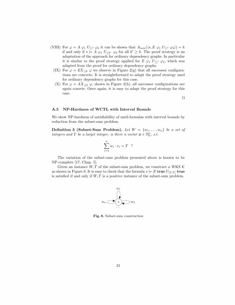
A.5 NP-Hardness of WCTL with Interval Bounds

We show NP-hardness of satisfiability of until-formulas with interval bounds byreduction from the subset-sum problem.

Definition 3 (Subset-Sum Problem). Let W = {w1, . . . , wn} be a set ofintegers and T be a target integer, is there a vector x ∈ Nn0 , s.t.

n∑i=1

wi · xi = T ?

The variation of the subset-sum problem presented above is known to beNP-complete [17, Chap. 5].

Given an instance W,T of the subset-sum problem, we construct a WKS Kas shown in Figure 8. It is easy to check that the formula s |= E true U[T,T ] trueis satisfied if and only if W,T is a positive instance of the subset-sum problem.

s

w1

w2

. . .

wn

Fig. 8. Subset-sum construction

31