Local Mixtures and Exponential Dispersion Models

Local Mixtures and Exponential Dispersion

Models

by

Paul Marriott

Department of Statistics & Applied Probability,

National University of Singapore,

3 Science Drive 2,

Singapore 117543.

email: [email protected]

Summary

Exponential dispersion models are powerful tools for modelling. They are

highly flexible yet they keep within a well understood inferential framework. This

paper looks at mixtures of exponential models, in particular local mixtures. It

considers the relationship between mixing and over-dispersion. By using geomet-

ric methods a new class of models is developed all of which are identifiable, flexible

and interpretable. A powerful large sample inference theory, especially suited to

families with boundaries, is developed which extends the good inferential proper-

ties of exponential dispersion families to the new class of mixture models.

Some key words: Affine geometry; Convex geometry; Differential geometry;

Dispersion model; Mixture model; Multinomial approximation; Statistical mani-

fold.

1

1 Introduction

Exponential dispersion models have proved to be very successful at increasing

modelling flexibility while keeping within a well understood inferential framework.

An excellent treatment of their theory and application can be found in Jørgensen

(1997). Another way of enriching a simple parametric modelling framework is

to consider mixing over parameters. This approach has many applications, see

for example see Titterington et al (1985), Lindsay (1995) or McLachlan & Peel

(2000). Marriott (2002, 2003) considers a restricted form of mixing, called local

mixing, which allows a considerable increase in inferential tractability compared

to general mixture models. This paper extends the theory of local mixing to

general exponential models. It introduces a new class of models called true local

mixtures whose members are flexible, identifiable, interpretable. Furthermore the

class has a tractable asymptotic inference theory which means that these models

are straightforward, if non-standard, inferentially.

This paper considers local mixtures for models of the exponential dispersion

form

fZ(z|θ, λ) := exp[λ{zθ − κ(θ)}]νλ(z)

where νλ(z) is independent of θ, see Jørgensen (1997, page 72). However all results

can also be easily extended to the additive form of dispersion models

exp{θz − λκ(θ)}νλ(z).

Throughout the measure νλ(z) is suppressed in the notation to aid clarity except

when it becomes important in the analysis.

The paper is organized as follows. Section 2 introduces the idea of a true local

mixture model and the examples used throughout. Section 3 discusses identifi-

cation and parameterisation issues for these models, while §4 considers inference.

In particular Theorem 4 describes a large sample asymptotic theory which makes

the models inferentially extremely tractable, while simulation studies illustrate the

relationship between local mixture models and other methods of dealing with over

dispersion. All proofs can be found in the appendix.

2

2 Local mixture models

Consider the following mixtures

∫

exp[λ{(θ + η)z − κ(θ + η)}]dQ(η) (1)

and∫

exp (λ{θ(µ + η)z − κ{θ(µ + η)}]) dQ(η), (2)

where Q is a distribution function. In (2) the mixing is over the mean value

parameterisation where µ(θ) is the expected value of Z under the parameters θ, λ.

The essential idea of a local mixture model is that the mixing is only responsible

for a relatively small amount of the variation in the model. Loosely it assumes

that the mixing distribution Q(η) in (1) and (2) is close to a delta function and

then applies a Laplace expansion. Using the expansions of Marriott (2002), under

regularity, these integrals can be approximated by low dimensional parametric

families. For the mixture given by integral (1) this approximation is

fZ(z|θ, λ)

(

1 + λξ1

{

z −d

dθκ(θ)

}

+ λξ2

−d2

dθ2κ(θ) + λz2 − 2 λ z

d

dθκ(θ) + λ

{

d

dθκ(θ)

}2

, (3)

with a positivity condition which ensures that (3) is a density given by

ξ12 − 4 ξ2 + 4 ξ2

2λd2

dθ2κ(θ) < 0.

As shown in Marriott (2002) the local mixture expansion is invariant with re-

spect to reparameterisation. Thus the same result as (3) is given by expanding inte-

gral (2) in the µ parameterisation. This expansion is denoted by fZ(z|θ(µ), λ, ν1, ν2)

which is defined by

fZ(z|θ(µ), λ)

[

1 + ν1

{

z − µ

V (µ)

}

+ ν2

−V (µ) + z2 − 2 µ z + µ2 − ddµ

V (µ)z + ddµ

V (µ)µ

V (µ)2

,(4)

3

where V (µ) is the variance function for the fZ(z|θ(µ), λ) family, see Jørgensen

(1997, pp48). The relationship between the parameters (ξ1, ξ2) and (ν1, ν2) can be

calculated directly from the chain rule and is given by

ν1 = ξ1∂µ

∂θ+ ξ2

∂2µ

∂θ2, ν2 = ξ2

(

∂µ

∂θ

)2

.

In general there are two issues to consider when using such models. First iden-

tification, since it is not clear that the parameters (µ, λ, ν1, ν2) of (4) uniquely char-

acterize densities. The second issue is the inferential implications of the boundary

which are an intrinsic part of such models. This paper treats both these issues.

2.1 True local mixture models

Investigation of the geometry of the local mixture expansion reveals a surprising

fact. Expansions of the form (3) and (4) need not themselves be mixture models.

If a model is a mixture it must satisfy some natural inequalities in its moment

structure. However, as is shown in the examples below, it is possible to find

parameter values (µ, λ, ν1, ν2) which generate a proper density which fails to respect

these natural mixture inequalities.

In order to see when the local mixture expansion can be interpreted as a mixture

define the subclass of local mixture models, called true local mixture models, for

which there exists a mixing distribution, Q̃, such that

fZ{z|θ(µ), λ, ν1, ν2} =∫

fZ{z|θ(µ + η), λ}dQ̃(η). (5)

Note the differences between equation (5) and the expansion given by (4). First,

equation (5) is not an asymptotic approximation, rather it is an equation which

requires the existence of Q̃. Second, the point θ(µ) need not be the mode of Q̃

as in the Laplace based expansion of Marriott (2002). Finally it is convenient to

define a subclass of mixing distributions. Define a true local mixture model to be

of width 2ε if the support of Q̃ lies in [−ε, ε]. This is a crude way of ensuring that

the mixing distribution is ‘small’.

4

2.2 Examples

In this section the examples are considered which are used throughout.

Example: Normal mixture family.

Consider a mixture over the mean parameter µ in a normal family with fixed

variance, known to be 1. That is

fZ(z|µ, Q) :=∫

φ(z|µ + η, 1)dQ(η),

where Q is a localizing mixture family and φ(z|µ, σ2) is the normal density with

mean µ and variance σ2. The corresponding local mixture density is

fZ(z|µ, 1, ν1, ν2) = φ(z|µ, 1)[

1 + ν1(z − µ) + ν2{(z − µ)2 − 1}]

,

and the positivity constraint which ensures that the expansion is a density is given

by

ν21 − 4ν2 + 4ν2

2 < 0. (6)

Under fZ(z|µ, Q), Z has a second moment greater than 1+{EQ(µ+η)}2, however

the moments of the corresponding local mixture model fZ(z|µ, 1, ν1, ν2) are

E(Z) = µ + ν1,

E(Z2) = 1 + (µ + ν1)2 + 2ν2 − ν2

1 .

Thus the natural moment structure for mixing implies the inequality

2ν2 − ν21 ≥ 0. (7)

Inspection shows that there are parameter values which satisfy inequality (6) but

not (7). Thus a necessary condition for fZ(z|µ, 1, ν1, ν2) to be a true local mixture

is that both (6) and (7) hold. It is shown later that this is also a sufficient condition

for small enough mixing.

Example: Poisson mixture family.

Consider the family of Poisson distributions parameterised by θ

Po(z|θ) =1

z!exp {zθ − exp(θ)} ,

5

where z ∈ IN . The local mixture family for this case has the form

Po(z|θ){

1 + ξ1

(

z − eθ)

+ ξ2

(

−eθ + z2 − 2 zeθ + e2 θ)}

,

with a positivity condition sufficient to ensure that this a density given by

ξ12 + 4 ξ2

2eθ − 4 ξ2 < 0.

As with the normal case this condition is not sufficient to ensure that the local

mixture is a true local mixture.

Example: Binomial mixture family.

The binomial family,

Bi(z|π, n) =n! πz (1 − π)n−z

z! (n − z)!,

has a local mixture expansion fZ(z|π, n, ν1, ν2) given by

Bi(z|π, n)

{

1 + ν1(z − π n)

π (1 − π)+ ν2

(z2 − z + 2 zπ − 2 zπ n + π2n2 − π2n)

π2 (π − 1)2

}

.

The positivity condition checks if there are any integers between 0 and n for which

the local mixture expression is negative. Thus there are n linear constraints of the

form

1 + ν1(z − π n)

π (1 − π)+ ν2

(z2 − z + 2 zπ − 2 zπ n + π2n2 − π2n)

π2 (π − 1)2 ≥ 0

for all z ∈ {0, · · · , n}. As with the other examples these conditions do not ensure

that the local mixture is a true local mixture. Conditions which do ensure this are

given later.

3 Identification and reparametrisation

3.1 Visualising the geometry

The key geometric idea in Marriott (2002) is that a local mixture family is an

embedded finite dimensional manifold with boundary. Hence it has good geometric

6

properties which can be exploited for inference. The geometric structure of the

family is discovered by considering its embedding in an infinite dimensional affine

space (XMix, VMix), where for all sufficiently smooth, square integrable f(z)

XMix ={

f(z)|∫

f(z)dν = 1}

, VMix ={

f(z)|∫

f(z)dν = 0}

,

see Marriott (2002) for details. The geometry of affine spaces is simple and

tractable, hence all calculations are made relative to this space.

Rather than go through the formal geometric arguments it might be more

helpful to consider the model visually. This might seem to be difficult since the

affine space (XMix, VMix) is infinite dimensional, but a lot of information can be

gathered by taking finite dimensional affine projections of this space. To do this

consider the following result.

Theorem 1 Define, for any integers (n1, n2, n3) for which the corresponding in-

tegrals converge, the map

(XMix, VMix) → IR3

fZ(z) 7→ (Ef(Zn1), Ef (Z

n2), Ef(Zn3)).

This map has the property that finite dimensional affine subspaces in (XMix, VMix)

map to finite dimensional affine subspaces in IR3.

Proof See Appendix

This theorem allows finite dimensional projections of (XMix, VMix) to be taken.

These projections respect the geometric structure. If a line is straight in (XMix, VMix)

it will automatically be straight in the projection. Furthermore, a point which lies

in a convex hull in (XMix, VMix) will lie in the convex hull of the image in IR3.

Thus, as far as possible, the visual geometry in the plot respects the geometry in

the infinite dimensional space.


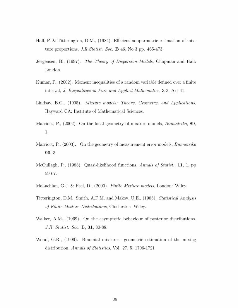
Figure 1 shows how the example of local mixtures of the normal family can

be visualised. The curve in Fig. 1 is the image of the family φ(z|µ, 1) in a three

7

dimensional representation given by the first three non-central moments. The two

arrows are the tangent and mixture curvature vectors for this family.

3.2 Orthogonal parameterisations

Theorem 9 of Marriott (2002) shows that any member of the local mixture family

can be written as an affine combination of the tangent and second derivative vec-

tors, translated so that the origin is moved to fZ(z|θ(µ), λ). It is a member of the

affine space

A(µ) :=

⟨

∂

∂µfZ(z|θ(µ), λ),

∂2

∂µ2fZ(z|θ(µ), λ)

⟩

fZ(z|θ(µ),λ)

,

where the notation 〈v1, v2〉x denotes the affine space through x spanned by v1, v2.

The positivity condition for any family defines a convex subset of this affine plane

within which lie all the local mixture models which are densities. Define the convex

subset of the affine space A(µ) by

F (µ) := {fZ(z|µ, λ, ν1, ν2) ∈ A(µ)|fZ(z|µ, λ, ν1, ν2) is a density } .

The full local mixture family is the union of all F (µ) as µ varies.


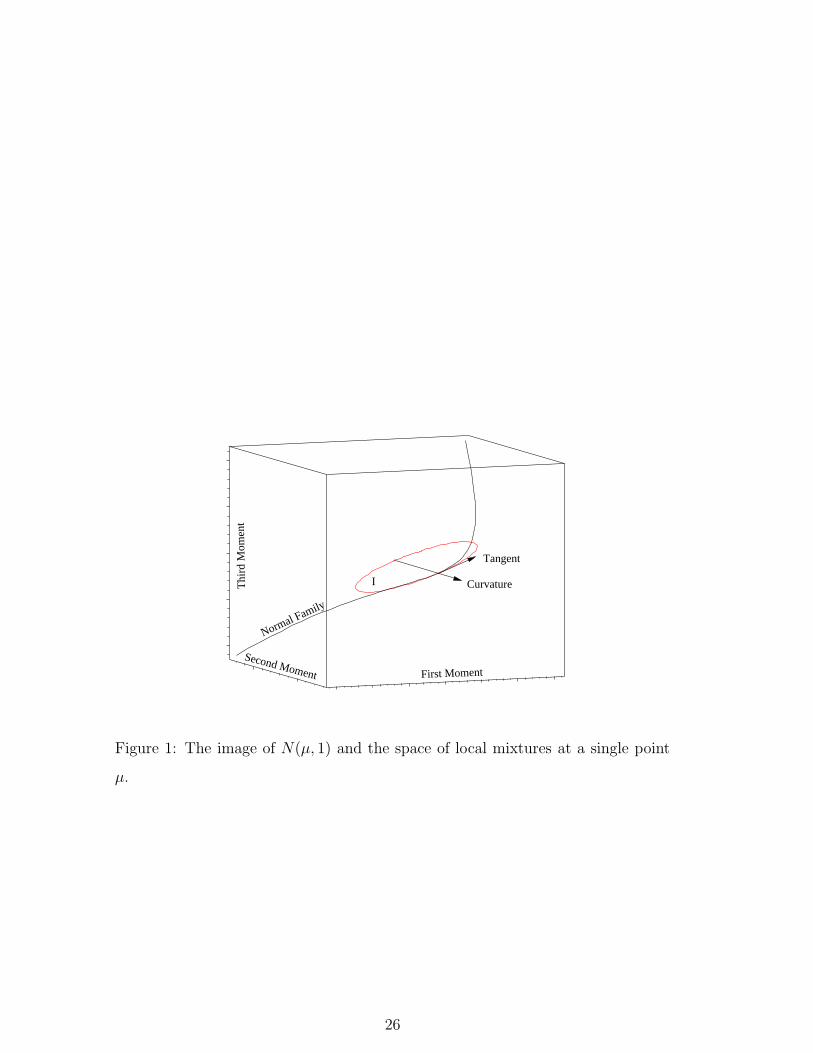
For the normal example one of the sets F (µ) is shown in Fig. 1 and denoted

by I. The union of all such families is shown in Fig. 2. It can be seen that

local mixtures are represented by the three dimensional interior of a smooth two

dimensional surface.

As is seen visually in Fig. 1, and is generally true, the tangent space to F (µ) and

the curve fZ(z|θ(µ), λ) share a common tangent direction, ∂∂µ

fZ(z|θ(µ), λ). This

is both geometrically and statistically inconvenient since it introduces problems

with identification and produces a singularity in the parameterisation. Hence it is

natural to reparametrise the model fZ(z|µ, λ, ν1, ν2) by (µ′, λ′, ν ′1, ν

′2) so that: (i)

ν ′1 = ν ′

2 = 0 corresponds to the family fZ(z|µ, λ) in the natural way, and (ii) that

8

for fixed µ′ and λ′ the two-dimensional sub-manifold defined by {fZ(z|µ′, λ′, ν ′1, ν

′2)}

is orthogonal to ∂∂µ

fZ(z|µ, λ, 0, 0).

For any exponential dispersion family the directions ∂∂η

and ∂∂µ

are Fisher or-

thogonal if∫ (z − µ)

V (µ)

∂fZ

∂η{z|µ(η), λ, ν1(η), ν2(η)} dz = 0

This holds if E(Z) is a constant in the ∂∂η

direction. Since the first moment for

Z with density fZ(z|µ, λ, ν1, ν2) is µ + ν1 it is required to find a parameterisation

(µ′, λ′, ν ′1, ν

′2) such that µ′ + ν ′

1 = a constant, while respecting condition (i). This

can always be easily achieved.


A parameterisation which achieves this for the normal family is given by µ′ =

µ − ν1, λ′1 = λ1, ν

′1 = ν1, ν

′2 = ν2, with the positivity constraint

ν ′21 − 4ν ′

2 + 4ν ′22 < 0.

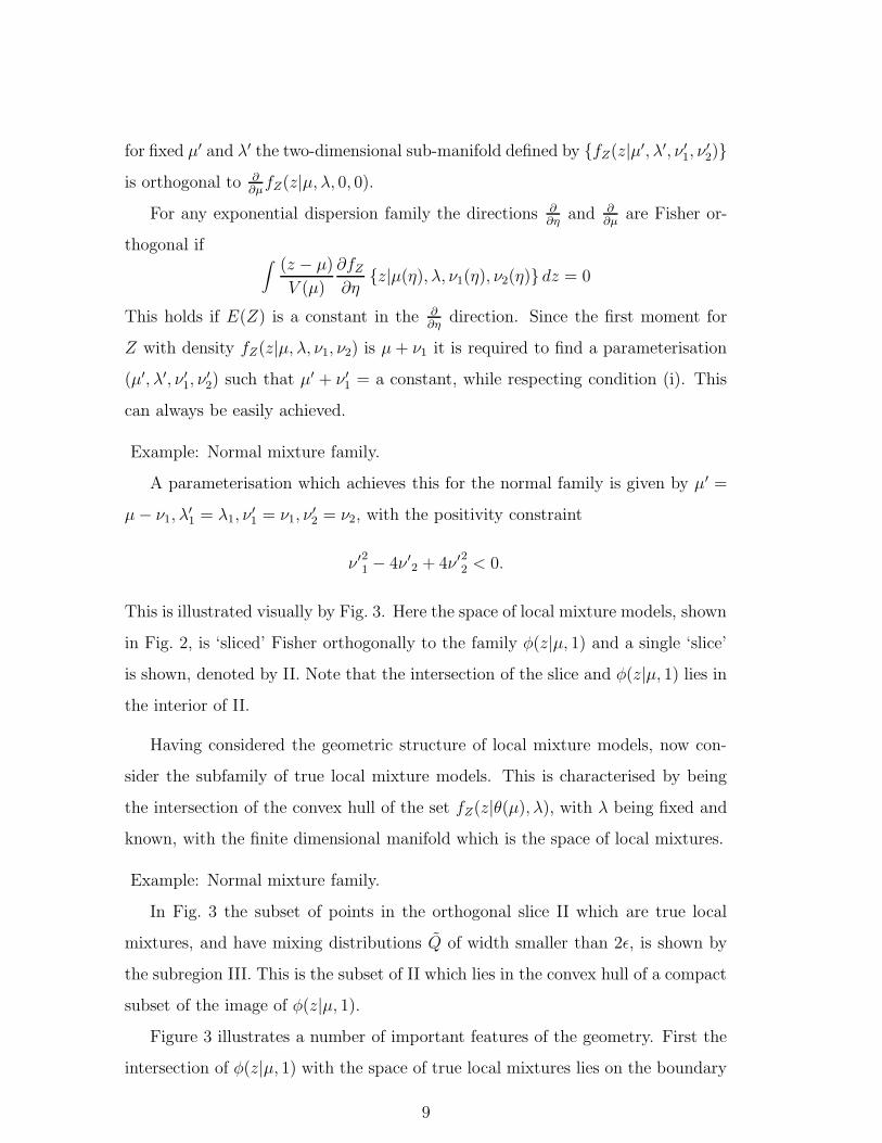
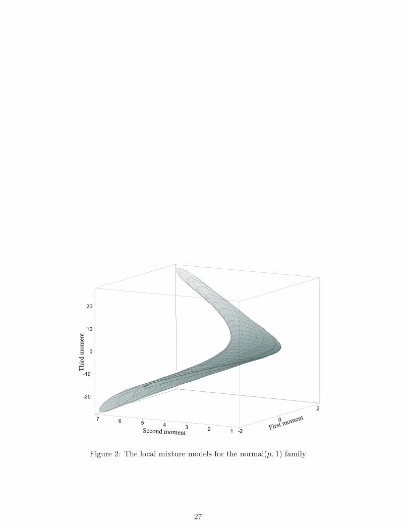
This is illustrated visually by Fig. 3. Here the space of local mixture models, shown

in Fig. 2, is ‘sliced’ Fisher orthogonally to the family φ(z|µ, 1) and a single ‘slice’

is shown, denoted by II. Note that the intersection of the slice and φ(z|µ, 1) lies in

the interior of II.

Having considered the geometric structure of local mixture models, now con-

sider the subfamily of true local mixture models. This is characterised by being

the intersection of the convex hull of the set fZ(z|θ(µ), λ), with λ being fixed and

known, with the finite dimensional manifold which is the space of local mixtures.


In Fig. 3 the subset of points in the orthogonal slice II which are true local

mixtures, and have mixing distributions Q̃ of width smaller than 2ε, is shown by

the subregion III. This is the subset of II which lies in the convex hull of a compact

subset of the image of φ(z|µ, 1).

Figure 3 illustrates a number of important features of the geometry. First the

intersection of φ(z|µ, 1) with the space of true local mixtures lies on the boundary

9

of this space. Any inference procedure must take this into account. Second note

that the boundary of III at the intersection is not smooth. If possible mixing

distributions, Q̃, are restricted to having a fixed compact support then the tangent

space of III is a tangent cone. The ‘angle’ that is made at the vertex of this cone

is a function of the size of the compact support of Q̃. The inferential consequences

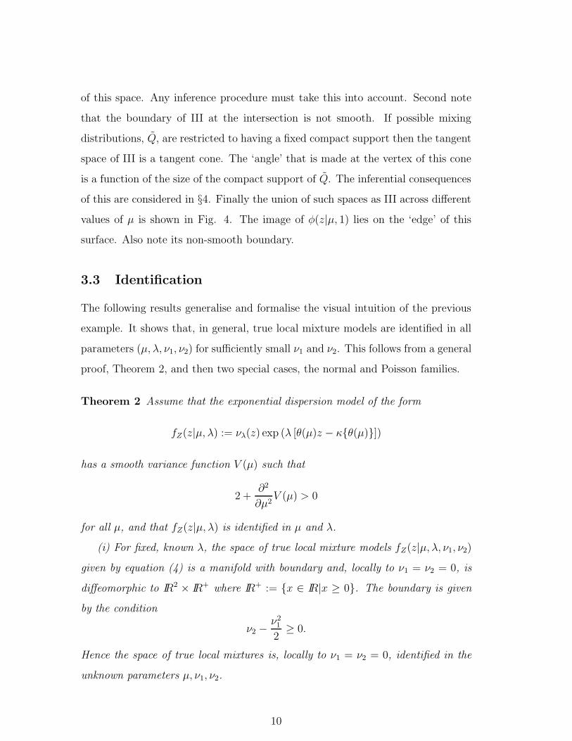
of this are considered in §4. Finally the union of such spaces as III across different

values of µ is shown in Fig. 4. The image of φ(z|µ, 1) lies on the ‘edge’ of this

surface. Also note its non-smooth boundary.

3.3 Identification

The following results generalise and formalise the visual intuition of the previous

example. It shows that, in general, true local mixture models are identified in all

parameters (µ, λ, ν1, ν2) for sufficiently small ν1 and ν2. This follows from a general

proof, Theorem 2, and then two special cases, the normal and Poisson families.

Theorem 2 Assume that the exponential dispersion model of the form

fZ(z|µ, λ) := νλ(z) exp (λ [θ(µ)z − κ{θ(µ)}])

has a smooth variance function V (µ) such that

2 +∂2

∂µ2V (µ) > 0

for all µ, and that fZ(z|µ, λ) is identified in µ and λ.

(i) For fixed, known λ, the space of true local mixture models fZ(z|µ, λ, ν1, ν2)

given by equation (4) is a manifold with boundary and, locally to ν1 = ν2 = 0, is

diffeomorphic to IR2 × IR+ where IR+ := {x ∈ IR|x ≥ 0}. The boundary is given

by the condition

ν2 −ν2

1

2≥ 0.

Hence the space of true local mixtures is, locally to ν1 = ν2 = 0, identified in the

unknown parameters µ, ν1, ν2.

10

(ii) For free, unknown λ, if

∂

∂λlog νλ(z) (8)

is not a polynomial in z then the space of true local mixture models is, locally to

ν1 = ν2 = 0, identified in all its parameters (µ, λ, ν1, ν2).

Proof See Appendix.

Note that the condition on the variance function of Theorem 2 appies to many

exponential dispersion families including the normal, Poisson, binomial, gamma,

extreme stable, compound Poisson, and many others, see Jørgensen (1997, page

130). However, while the condition in Theorem 2(ii) on the normalising factor

νλ(z) is quite general and applies to the binomial, gamma, negative binomial and

many other families, Jørgensen (1997, pp 85-91), there are two very important

special cases for which this condition does not hold. These are the normal and

Poisson families. These cases are treated here separately as they require a rather

more detailed analysis.


The well known fact that a mixture of normal distributions can itself be normal,

in particular that

∫

φ(z|µ + η, σ21)φ(η|0, σ2

2)dη = φ(z|µ, σ21 + σ2

2) (9)

makes one suspect that the identification issue for this family must be quite deli-

cate. Direct calculation shows that the condition in Theorem 2 (ii) does not hold.

Despite this, as is shown in the Appendix, locally to ν1 = ν2 = 0 the local mixture

family is fully identified in (µ, λ, ν1, ν2).

Example: Poisson mixture family.

Jørgensen (1997, p 90) shows how to write the Poisson family as an additive

exponential dispersion model,

λz

z!exp(θz − λ exp(θ)),

11

but also shows that this is the only family for which θ and λ are not identified,

since µ = λ exp(θ). Hence this family falls outside the regularity conditions of

Theorem 2. The relevant result for this family is that the true local mixture model

is identified for the three parameters µ, ν1, ν2, locally to ν1 = ν2 = 0.

To be consistent with the idea of local mixing it is interesting to see what effect

putting structure on the possible mixing distribution Q̃ has on the geometry. It is

natural to ask that Q̃ is small in some sense. This can be done in many ways and

one method is considered here and in more detail in §4.

For a true local mixture fZ(z|µ, λ, ν1, ν2) there exists a mixing distribution Q̃

such that fZ(z|µ, λ, ν1, ν2) =∫

fZ(z|µ+η, λ)dQ̃(η). By calculation of moments and

applying Taylor’s theorem the following identities follow easily

ν1 = EQ̃(η), (10)

ν2 =1

2EQ̃(η2) +

1

3!

V ′′′(µ∗)

2 + V ′′(µ)EQ̃(η3), (11)

where ′ denotes differentiation with respect to µ and µ∗ is some value in the interval

(µ, µ + ν1).

If the mixing distribution has finite support then, following Kumar (2002),

there are natural inequalities on all moments hence, from equations (10)-(11),

there are restrictions on the ν1 and ν2 parameters for each µ, λ. In particular

simple calculations show that for fixed µ and λ,

EQ̃(η2) ≤ ν21 + εν1.

Such a restriction is shown, for the normal example, in Fig. 5 on the space A3

defined in the proof of Theorem 2 and in the region III of Fig. 3. The shaded areas

show the subset of true local mixtures for which Q̃ has width 2ε. The following

theorem formalises this observation.

Theorem 3 Assume that an exponential dispersion model fZ(z|µ, λ) satisfies the

conditions of Theorem 2 and that Q̃, defined by equation (5), has finite support

and is of width 2ε.

12

(i) For fixed, known λ the sub-set of true local mixture models is a manifold

with boundary and locally to ν1 = ν2 = 0 is diffeomorphic to IR × IR+ × IR+.

(ii) For free λ if the conditions of Theorem 2 holds, or if the family is normal,

the family of true local mixtures, locally to ν1 = ν2 = 0, is diffeomorphic to IR2 ×

IR+ × IR+.

Proof See Appendix.

4 Inference

4.1 Boundaries and inference

As motivation for the basic principle of this section consider inference on ρ in the

simplest type of mixture model

ρf(z) + (1 − ρ)g(z) (12)

where f(z) and g(z) are known. Hall and Titteringon (1984) consider this problem

when f and g are unknown and the analysis below follows their approach in the

simpler case.

For this problem there are two types of boundary for ρ. First ρ has the in-

terpretation of being a probability, thus 0 ≤ ρ ≤ 1. Denote the extreme values 0

and 1 here as soft boundaries. Second since the expression g(z) + ρ(f(z) − g(z))

integrates to one for all ρ, (12) is a density if and only if it is non-negative for

all z. Let the set ρ for which (12) is a density be given by [ρmin, ρmax]. Denote

the boundary of [ρmin, ρmax] as a hard boundary. It is immediate that the soft

boundary lies always inside the hard boundary.

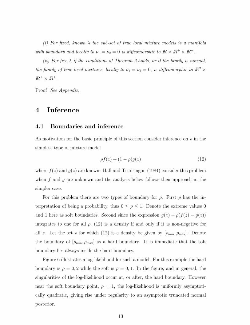
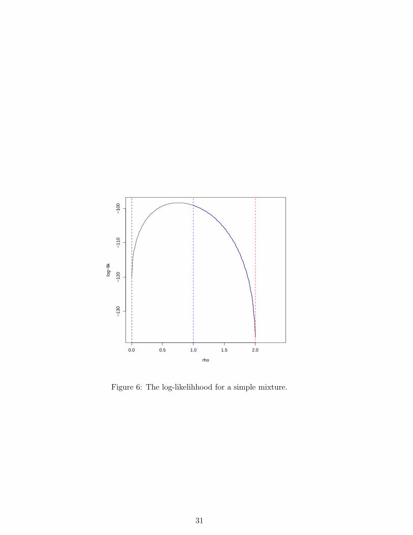
Figure 6 illustrates a log-likelihood for such a model. For this example the hard

boundary is ρ = 0, 2 while the soft is ρ = 0, 1. In the figure, and in general, the

singularities of the log-likelihood occur at, or after, the hard boundary. However

near the soft boundary point, ρ = 1, the log-likelihood is uniformly asymptoti-

cally quadratic, giving rise under regularity to an asymptotic truncated normal

posterior.

13

The critical condition for asymptotic truncated posterior normality is that the

soft boundary dominates the inference problem, either because it is stricter, or be-

cause the hard boundary is in an inferentially unimportant region of the parameter

space. Figure 6 illustrates both of these points. The soft boundary point ρ = 1 is

stricter than the hard boundary point ρ = 2, and although ρ = 0 is both hard and

soft it lies a long way in the tail of the posterior distribution. For this example

then a good approximation to a truncated normal posterior is expected.

This discussion can be generalised to true local mixture models. For this class

the boundaries are again of two forms. The hard boundaries come from the pos-

itivity conditions on the expansions (3) or (4). The soft boundaries come from

restricting to true local mixtures which lie within the convex hull of fZ(z|µ, λ).

If the bounds from the second of these conditions are stricter and bounded away

from the positivity bounds then approximately truncated quadratic log-likelihoods

and truncated normal posteriors should be expected. In general since a true local

mixture satisfies equation (5), the soft boundary lies inside the hard positivity

boundary. Detailed analysis of the examples in this paper shows that asymptoti-

cally the soft boundary is strictly inside the hard boundary and the hard boundary

is inferenicially asymptotically unimportant.

The following proof follows Hall and Titterington (1984) by embedding the

true local mixture model in a multinomial family in order to investigate the log-

likelihood approximation.

Theorem 4 Let fZ(z|µ, λ, ν1, ν2) be a true local mixture model which either satis-

fies the conditions of Theorem 2, or is a normal or Poisson family. Asymptotically,

in sample size, in any region strictly inside the hard boundary, the log-likelihood

is uniformly quadratic on (µ′, λ, α, β) in a shrinking neighbourhood of the mode,

where

µ′ = µ + ν1, α = 2ν2 − ν21 , β =

ν31

3− ν1ν2.

Furthermore, assuming any prior chosen is continuous then the posterior for (µ′, λ, α, β)

will be an asymptotically truncated normal distribution.

14

Proof See Appendix.

4.2 Examples

This section looks at examples of inference in a true local mixture model. In order

to keep the presentation focused it concentrates on over-dispersion and mixing in

the binomial example. The comparison of the normal and binomial cases illustrates

the fundamental differences between continuous and discrete distributional theory.

For an extensive treatment of the normal based examples see Marriott (2002, 2003).

There is a large literature regarding the problem of over-dispersion with bi-

nomial models and this section looks at a number of approaches. The geometric

approach taken here has strong links with that of Lindsay (1995) and in particular

with the related work of Wood (1999). Wood looks at the problem of learning about

the mixing distribution, Q. In contrast to this a practitioner might be interested in

estimating µ = E(Z), under an over-dispersed binomial model. Two approaches

are of interest here, quasi-likelihood and direct modelling through, for example,

the beta-binomial model. For the first of these approaches see Cox (1983), Mc-

Cullagh (1983) and Firth (1987) and references therein. For the second approach

see Crowder (1978). Finally one might be interested in testing for over-dispersion,

again see Cox (1983). This section demonstrates that for each of these possible

inferential questions the true local mixture approach is powerful, insightful and

computationally straightforward.

For computations with true local mixture models the Markov chain Monte Carlo

algorithm is use here. This is not the only possible approach, for example Marriott

(2003) uses a simple closed form geometrically based estimator, while Critchley and

Marriott (2003) use moment based methods. However the richness of the output

of Markov chain Monte Carlo gives the clearest illustration of the local mixture

approach. Furthermore Theorem 4 indicates that it is to be expected that the

performance of the algorithm will be extremely good. Finally, the algorithm allows

exploration of the effect of different prior assumptions on the form, in particular the

size, of the mixing distribution, and of the effect of the hard and soft boundaries.

15

Wood (1999) uses a geometric framework very similar to the one in §3.1. The

binomial family Bi(z|π, n) is embedded in the simplex,

Tn =

{

(x0, x1, . . . , xn) |n∑

i=1

xi = 1, xi ≥ 0 for all i

}

,

in IRn+1 by the mapping

(Bi(0|π, n), Bi(1|π, n), . . . , Bi(n|π, n)).

It is immediate that the affine space (XMix, VMix) used in this paper is isomorphic

to the hyperplane in IRn+1 which contains Tn. Thus for the binomial example the

affine geometry of this paper and Wood’s are identical.

Consider an example motivated by Example 1 of Wood (1999, p. 1715). In

this example data was generated from a Bi(z|π, n) distribution where n = 10 and

π was drawn from a distribution with mean 0.5 and a small standard deviation.

Using a large simulated dataset Wood shows that the mixing distribution can be

estimated from such data. Such an example can be thought of as a local mixture.

Using Wood’s example as motivation consider a much smaller dataset, with sample

size 50, generated from his fitted distribution. Here π comes from the discrete dis-

tribution with support at (0.46, 0.47, 0.48, 0.49, 0.50, 0.51, 0.52, 0.53) with probabil-

ities (0.0116, 0.0881, 0.1430, 0.1759, 0.1865, 0.1745, 0.1394, 0.0810). Since the sam-

ple size is so much smaller than Wood’s it is unrealistic to expect that the full

mixing distribution can be estimated. Rather the local mixture methodology in-

stead estimates the parameters in fZ(z|π, ν1, ν2).

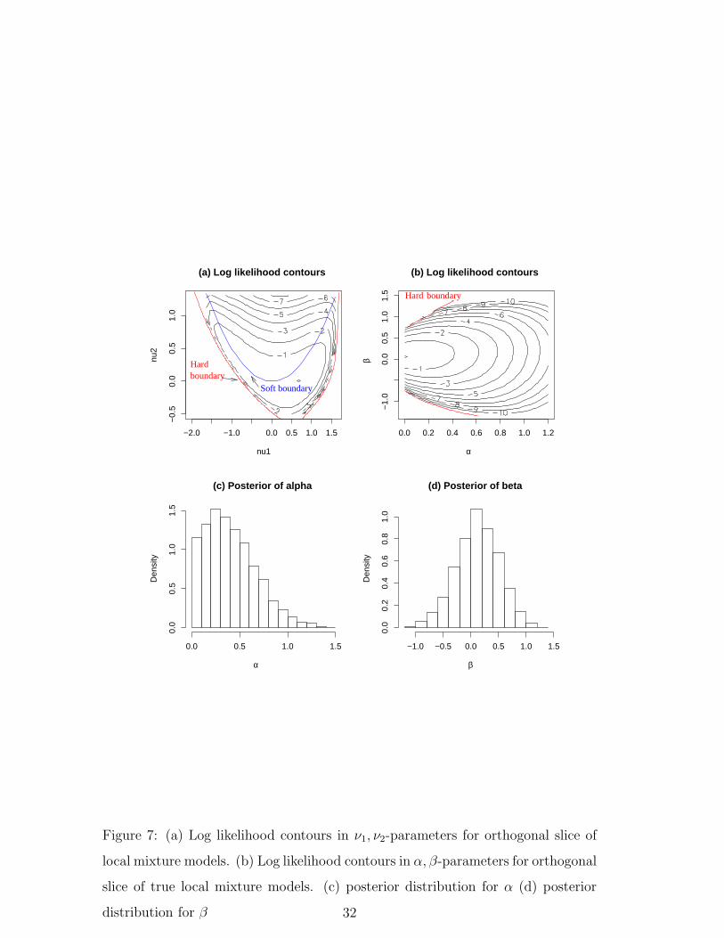
Figure 7 shows the log likelihood function for this dataset for the slice of the

space of true local mixtures which is orthogonal to Bi(z|π, n) at the sample mean.

Figure 7 (a) shows the log likelihood in the (ν1, ν2) parameterisation while 7 (b)

shows the log likelihood contours for the (α, β) parameterisation. This parameter-

isation,

(α, β) :=

(

ν2 −ν2

1

2,ν3

1

3− ν1ν2

)

.

was used in Theorems 2 and 4 and shown in Fig. 5. In Fig. 7 (a) the hard

boundary given by the intersection of the slice with the boundary of Tn can clearly

16

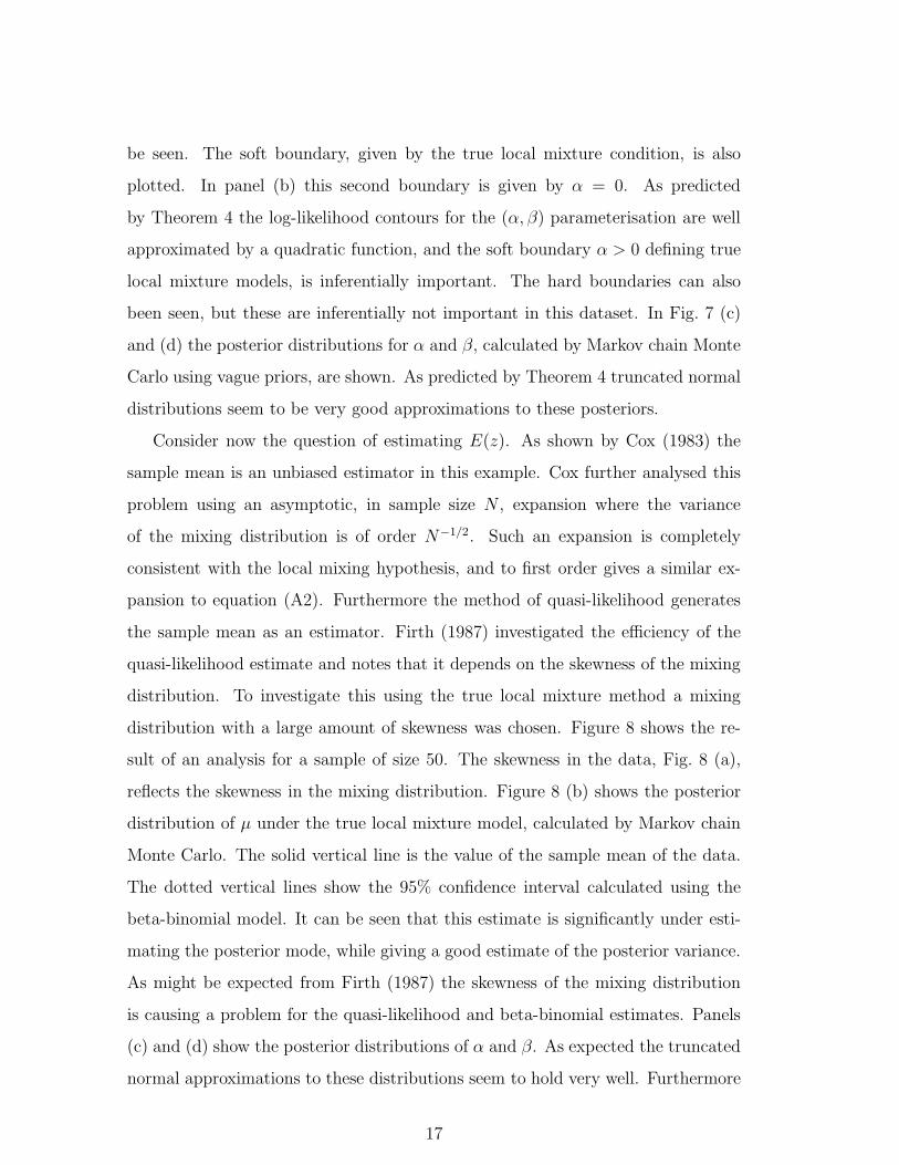
be seen. The soft boundary, given by the true local mixture condition, is also

plotted. In panel (b) this second boundary is given by α = 0. As predicted

by Theorem 4 the log-likelihood contours for the (α, β) parameterisation are well

approximated by a quadratic function, and the soft boundary α > 0 defining true

local mixture models, is inferentially important. The hard boundaries can also

been seen, but these are inferentially not important in this dataset. In Fig. 7 (c)

and (d) the posterior distributions for α and β, calculated by Markov chain Monte

Carlo using vague priors, are shown. As predicted by Theorem 4 truncated normal

distributions seem to be very good approximations to these posteriors.

Consider now the question of estimating E(z). As shown by Cox (1983) the

sample mean is an unbiased estimator in this example. Cox further analysed this

problem using an asymptotic, in sample size N , expansion where the variance

of the mixing distribution is of order N−1/2. Such an expansion is completely

consistent with the local mixing hypothesis, and to first order gives a similar ex-

pansion to equation (A2). Furthermore the method of quasi-likelihood generates

the sample mean as an estimator. Firth (1987) investigated the efficiency of the

quasi-likelihood estimate and notes that it depends on the skewness of the mixing

distribution. To investigate this using the true local mixture method a mixing

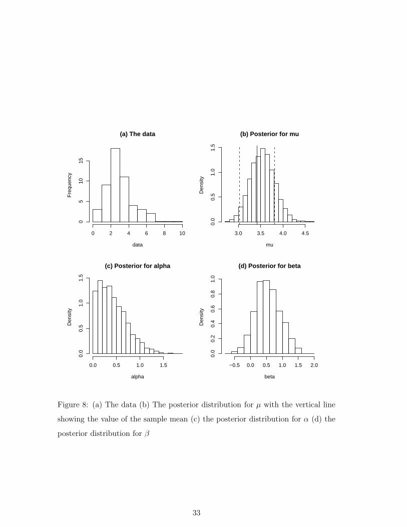
distribution with a large amount of skewness was chosen. Figure 8 shows the re-

sult of an analysis for a sample of size 50. The skewness in the data, Fig. 8 (a),

reflects the skewness in the mixing distribution. Figure 8 (b) shows the posterior

distribution of µ under the true local mixture model, calculated by Markov chain

Monte Carlo. The solid vertical line is the value of the sample mean of the data.

The dotted vertical lines show the 95% confidence interval calculated using the

beta-binomial model. It can be seen that this estimate is significantly under esti-

mating the posterior mode, while giving a good estimate of the posterior variance.

As might be expected from Firth (1987) the skewness of the mixing distribution

is causing a problem for the quasi-likelihood and beta-binomial estimates. Panels

(c) and (d) show the posterior distributions of α and β. As expected the truncated

normal approximations to these distributions seem to hold very well. Furthermore

17

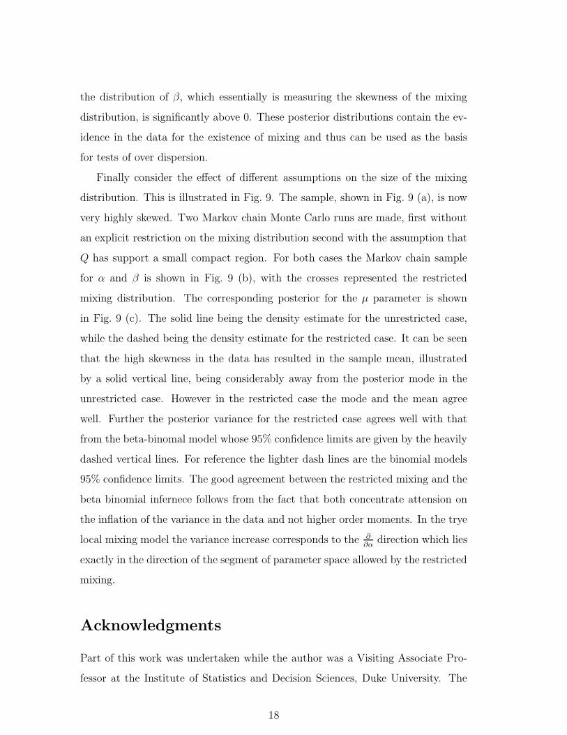
the distribution of β, which essentially is measuring the skewness of the mixing

distribution, is significantly above 0. These posterior distributions contain the ev-

idence in the data for the existence of mixing and thus can be used as the basis

for tests of over dispersion.

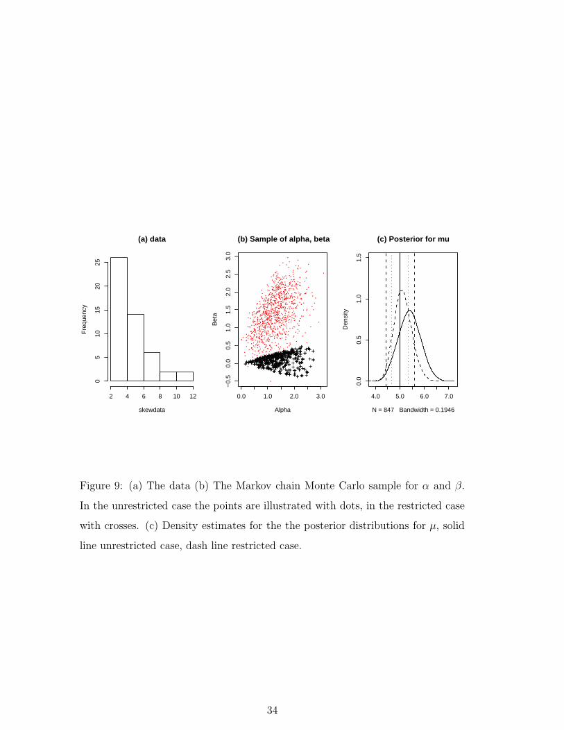
Finally consider the effect of different assumptions on the size of the mixing

distribution. This is illustrated in Fig. 9. The sample, shown in Fig. 9 (a), is now

very highly skewed. Two Markov chain Monte Carlo runs are made, first without

an explicit restriction on the mixing distribution second with the assumption that

Q has support a small compact region. For both cases the Markov chain sample

for α and β is shown in Fig. 9 (b), with the crosses represented the restricted

mixing distribution. The corresponding posterior for the µ parameter is shown

in Fig. 9 (c). The solid line being the density estimate for the unrestricted case,

while the dashed being the density estimate for the restricted case. It can be seen

that the high skewness in the data has resulted in the sample mean, illustrated

by a solid vertical line, being considerably away from the posterior mode in the

unrestricted case. However in the restricted case the mode and the mean agree

well. Further the posterior variance for the restricted case agrees well with that

from the beta-binomal model whose 95% confidence limits are given by the heavily

dashed vertical lines. For reference the lighter dash lines are the binomial models

95% confidence limits. The good agreement between the restricted mixing and the

beta binomial infernece follows from the fact that both concentrate attension on

the inflation of the variance in the data and not higher order moments. In the trye

local mixing model the variance increase corresponds to the ∂∂α

direction which lies

exactly in the direction of the segment of parameter space allowed by the restricted

mixing.

Acknowledgments

Part of this work was undertaken while the author was a Visiting Associate Pro-

fessor at the Institute of Statistics and Decision Sciences, Duke University. The

18

author would also like to thank Frank Critchley for many helpful discussions.

Appendix: Proofs of Theorems

Proof of Theorem 1

Any finite dimensional affine subspace in (XMix, VMix) can be defined by

f +∑

i

λivi,

where f ∈ XMix, vi ∈ VMix. The image of this space will therefore be in IR3,

(

Ef+∑

iλivi

(Zn1), Ef+∑

iλivi

(Zn2), Ef+∑

iλivi

(Zn3))

Expanding gives

(Ef(Zn1), Ef(Z

n2), Ef(Zn3)) +

∑

i

λi (Evi(Zn1), Evi

(Zn2), Evi(Zn3)) .

which is an affine space, when all integrals exist. 2

Proof of Theorem 2.

First consider the following lemma.

Lemma If the Fisher information at µ is non zero for the family

fZ(z|µ, λ) := eλ θ(µ) z−λκ{θ(µ)},

and if l 6= k, then∂l

∂µlfZ(z|µ, λ) and

∂k

∂µkfZ(z|µ, λ)

are linearly independent as functions of z.

Proof . First consider ∂l

∂θl fZ(z|θ, λ) which has the form Pl(z)fZ(z|θ, λ) where Pl(z)

is a polynomial in z of order l with leading coefficient λl. It is immediate that

∂l

∂θlfZ(z|θ, λ) and

∂k

∂θkfZ(z|θ, λ)

are linearly independent as functions of z when l 6= k.

19

The derivative ∂l

∂µl fZ(z|µ, λ) can be calculated from the chain rule and has the

form Pl(z)fZ(z|µ, λ), now with the leading term having the coefficient λl(

∂θ∂µ

)l.

This is non zero if the Fisher information is non zero and the result follows. 2

(i) Having proved the lemma now assume that fZ(z|µ, λ) satisfies the conditions

of the theorem. Any local mixture model with mean µ0 has the form

fZ(z|µ0 − ν1, λ) + ν1∂

∂µfZ(z|µ0 − ν1, λ) + ν2

∂2

∂µ2fZ(z|µ0 − ν1, λ) (A1)

whose tangent directions ∂∂ν1

and ∂∂ν2

are orthogonal to ∂∂µ

when ν1 = ν2 = 0.

Hence it is sufficient to examine the identification of expression (A1) for ν1 and ν2

and a fixed mean, µ0.

All local mixtures lie in the affine space (XMix, VMix), thus can be written as

fZ(z|µ0, λ) + V (z)

where V (z) ∈ VMix. Let Vpower(µ0) be the vector subspace of VMix defined by the

set of all formal power series

∞∑

k=1

C(k)∂k

∂µkfZ(z|µ0, λ)

where C(k) is independent of z, and let Xpower(µ0) be the set of functions of the

form

Xpower := {fZ(z|µ0, λ) + v | v ∈ Vpower(µ0)} .

By expanding (A1) by Taylor’s theorem it follows that locally to fZ(z|µ0, λ) it has

the form

fZ(z|µ0, λ)+

(

ν2 −ν2

1

2

)

∂2

∂µ2fZ(z|µ0, λ)+

(

ν31

3− ν1ν2

)

∂3

∂µ3fZ(z|µ0, λ)+

∑

l≥4

Cl∂l

∂µlfZ(z|µ0, λ).

(A2)

and lies in the affine space (XPower(µ0), VPower(µ0)). By the lemma the higher order

terms in the sum are linearly independent of the first three terms. Hence there ex-

ists a well defined affine map from (XPower(µ0), VPower(µ0)) into the two dimensional

affine space

A3(µ, λ) :=

⟨

∂2

∂µ2fZ(z|µ0, λ),

∂3

∂µ3fZ(z|µ0, λ)

⟩

fZ(z|µ0,λ)

20

defined by dropping the higher order terms. To prove identification in (XMix, VMix)

it is sufficient to prove it in this finite dimensional subspace. Using the obvious

coordinate system, the image of the local mixtures is given by

(α, β) :=

(

ν2 −ν2

1

2,ν3

1

3− ν1ν2

)

and Fig. 5 shows this image directly.

Under the condition on the variance function and by using Jensen’s inequality,

any true local mixture fZ(z|µ0, λ, ν1, ν2) satisfies the moment inequality

EfZ(z|µ0,λ)(Z2) ≤ EfZ(z|µ0−ν1,λ,ν1,ν2)(Z

2).

Expanding the right hand side as a series in ν1, ν2 gives

µ20 + V (µ0) +

{

2 +∂2

∂µ2V (µ)

}{

ν2 −ν2

1

2

}

+ · · · .

Thus, for sufficiently small, ν1, ν2 it is a necessary condition for being a true local

mixture that

ν2 −ν2

1

2> 0. (A3)

In Fig. 5 this region is shown by the half plane, α > 0. Analysis shows that in this

region the coordinate system (α, β) is non singular, and has a point singularity

only on α = 0 at the origin ν2 = 0.

To show that the condition is sufficient to give a true local mixture consider

the convex hull of the image of fZ(z|µ, λ) in the affine space defined the first three

deriatives

⟨

∂

∂µfZ(z|µ0, λ),

∂2

∂µ2fZ(z|µ0, λ),

∂3

∂µ3fZ(z|µ0, λ)

⟩

fZ(z|µ0,λ)

.

At µ0 the image is given by truncating the Taylor expansion to

fZ(z|µ0, λ) +3∑

i=1

1

i!(µ − µ0)

i ∂i

∂µifZ(z|µ0, λ).

Any two component mixture

πfZ(z|µ0 + µ1, λ) + (1 − π)fZ(z|µ0 + µ2, λ)

21

which satisfies the constraint that its mean is µ0 has an image in the (α, β) pa-

rameterisation, defined above, given by (−µ1µ2,−(µ1 + µ2)µ1µ2). Hence since the

projection of the convex hull of fZ(z|µ, λ) in (XMix, VMix) is onto the convex hull

of the projection of fZ(z|µ, λ) in A3(µ, λ) it is clear that that true local mixtures,

in the (α, β) parameterisation, spans IR+ × IR.

The space of tangent vectors for fZ(z|µ, λ, ν1, ν2) at ν1 = ν2 = 0 is therefore

an orthogonal sum of the tangent space ∂∂µ

and that of ∂∂ν1

and ∂∂ν2

which has the

form IR × IR+. Locally to ν1 = ν2 = 0 the space of true local mixture models is a

manifold with boundary and is locally diffeomorphic to IR2 × IR+.

(ii) If λ is now considered a free parameter the identification of 4 parameters

needs to be considered. It is sufficient to show that the tangent vector

∂

∂λfZ(z|µ, λ)

does not lie in the space spanned by ∂∂µ

, ∂∂ν1

, ∂∂ν2

of fZ(z|µ, λ, ν1, ν2) at ν1 = ν2 = 0.

By direct calculation it can be seen that each element of this space can be written

as P (z)fZ(z|µ, λ) where P (z) is a polynomial in z. Since, under the assumption

of the theorem the tangent vector

∂

∂λfZ(z|µ, λ) =

[

∂

∂λlog{νλ(z)} + θz − κ(θ)

]

fZ(z|µ, λ)

is not of this form it follows that it does not lie in the tangent space of the other

parameters. Hence locally to ν1 = ν2 = 0 the family fZ(z|µ, λ, ν1, ν2) is identified.

2

Proof of identification in normal example.

As in the proof of Theorem 2 consider for some value µ0 the subset of local

mixture models which have E(z) = µ0. As above the image of this set in the affine

space

A4(µ, σ2) :=

⟨

∂2

∂µ2fZ(z|µ0, σ

2),∂3

∂µ3fZ(z|µ0, σ

2),∂4

∂µ4fZ(z|µ0, σ

2)

⟩

fZ(z|µ0,σ2)

is

fZ(z|µ0, σ2) +

(

ν2 −ν2

1

2

)

∂2

∂µ2fZ(z|µ0, σ

2) +

(

ν31

3− ν1ν2

)

∂3

∂µ3fZ(z|µ0, σ

2)

22

+

(

ν21ν2

2−

ν41

8

)

∂4

∂µ4fZ(z|µ0, σ

2).

By expanding this as a Taylor series around σ20 it can be seen that the projection

into A4 is well defined and given by

fZ(z|µ0, σ20) +

(

δ

2+ ν2 −

ν21

2

)

∂2

∂µ2fZ(z|µ0, σ

20)

+

(

ν31

3− ν1ν2

)

∂3

∂µ3fZ(z|µ0, σ

20)

+

(

δ2

8+

δ

2(ν2 −

ν21

2) +

ν21ν2

2−

ν41

8

)

∂4

∂µ4fZ(z|µ0, σ

20)

where σ2 = σ20 + δ. In the obvious coordinates this can be written as

(

α +δ

2, β,

δ2

8+

δ

2α −

1

4C(α, β)2α −

3

4C(α, β)β

)

where when α ≥ 0 C(α, β) is a well-defined function. The map from α, β, δ to this

space can easily be shown to be one to one when α ≥ 0. 2

Proof of Theorem 3.

As shown in the proof of Theorem 2 the subset of the space of true local

mixtures orthogonal to ∂∂µ

at µ0 is, locally to ν1 = ν2 = 0, diffeomorphic to a

subset of A3(µ0, λ). If the mixing distribution is of width 2ε this is diffeomorphic

to the convex hull of (x2, x3) for |x| ≤ ε. The result follows immediately. 2

Proof of Theorem 4

Standard proofs of the asymptotic normality of the posterior, for example

Walker (1969), can almost be applied directly, except for the fact that the pa-

rameter space is not an open subset of IR4. When the conditions of Theorem 2

apply, or the family is normal or Poisson, then the true local mixture family is

locally diffeomorphic to a closed segment

S = {(x, y, z, w) ∈ IR4|z, w ≥ 0},

in particular the boundary is typically inferentially important.

In order to return the inference to a more regular setting it is convenient to

embed the model in a larger one where standard results apply. Following Hall

23

and Titterington (1984) consider approximating the log-likelihood for a true local

mixture family by a multinomial approximation determined by the probabilities

(π1, · · · , πM), where the number of bins, M , in the multinomial model grows at

a rate N1/4, where N is the sample size. In such a family the log-likelihood is

uniformally quadratic in any neighbourhood strictly bounded away from the hard

boundaries πi = 0, 1.

The embedding is given by

(µ′, λ, α, β) → πi(µ′, λ, α, β) =

∫

Di

fZ(z|µ′, λ, α, β)dz.

The approximation of the log-likelihood relies on

log {fZ(zi|µ′, λ, α, β)|Dj|} − log

{

∫

Dj

fZ(z|µ′, λ, α, β)dz

}

→ 0 (A4)

as N → ∞, where zi ∈ Dj. By assumption the region of parameter space of

interest lies strictly inside the positivity boundary, thus fZ(zi|µ′, λ, α, β) is strictly

bounded away from zero hence the contribution to the log-likelihood remains finite

for all zi and the convergence in (A4) applies.

The posterior on (µ′, λ, α, β) is approximated by the posterior in IRM condi-

tionally on being on the image of (µ′, λ, α, β). Since this image is diffeomorphic to

S it is approximately a truncated normal. It follows by standard arguments that

the posterior is asymptotically truncated normal. 2

References

Cox, D.R., (1983). Some remarks on overdispersion, Biometrika, 70, 1, pp 269-74.

Critchley, F. & Marriott, P. (2003). Data-informed influence analysis, Under

review for Biometrika.

Crowder, M.J., (1978). Beta-binomial anova for proportions, Appl. Statist. 27,

No. 1, pp. 34-37.

Firth, D., (1987), On the efficiency of quasi-likelihood estimation, Biometrika,

74, 2, pp 233-45.

24

Hall, P. & Titterington, D.M., (1984). Efficient nonparmetric estimation of mix-

ture proportions, J.R.Statist. Soc. B 46, No 3 pp. 465-473.

Jørgensen, B., (1997). The Theory of Dispersion Models, Chapman and Hall:

London.

Kumar, P., (2002). Moment inequalities of a random variable defined over a finite

interval, J. Inequalities in Pure and Applied Mathematics, 3 3, Art 41.

Lindsay, B.G., (1995). Mixture models: Theory, Geometry, and Applications,

Hayward CA: Institute of Mathematical Sciences.

Marriott, P., (2002). On the local geometry of mixture models, Biometrika, 89,

1.

Marriott, P., (2003). On the geometry of measurement error models, Biometrika

90, 3.

McCullagh, P., (1983). Quasi-likelihood functions, Annals of Statist., 11, 1, pp

59-67.

McLachlan, G.J. & Peel, D., (2000). Finite Mixture models, London: Wiley.

Titterington, D.M., Smith, A.F.M. and Makov, U.E., (1985). Statistical Analysis

of Finite Mixture Distributions, Chichester: Wiley.

Walker, A.M., (1969). On the asymptotic behaviour of posterior distributions.

J.R. Statist. Soc. B, 31, 80-88.

Wood, G.R., (1999). Binomial mixtures: geometric estimation of the mixing

distribution, Annals of Statistics, Vol. 27, 5, 1706-1721

25

Normal Family

Tangent

CurvatureI

First MomentSecond Moment

Thi

rd M

omen

t

Figure 1: The image of N(µ, 1) and the space of local mixtures at a single point

µ.

26

-2

0

2

123

456

7

-20

-10

0

10

20

First moment

Second moment

Thir

d m

om

ent

Figure 2: The local mixture models for the normal(µ, 1) family

27

Thi

rd M

omen

t

Second Moment

Firs

t Mom

ent

Curvature

Tangent

Normal Family

II

III

Figure 3: The image of N(µ, 1) and the orthogonal slice of the space of local

mixture models. Region II shows the space of local mixtures with a fixed mean,

while the subregion III shows the true local mixtures whose mixing distribution

has a fixed compact support.

28

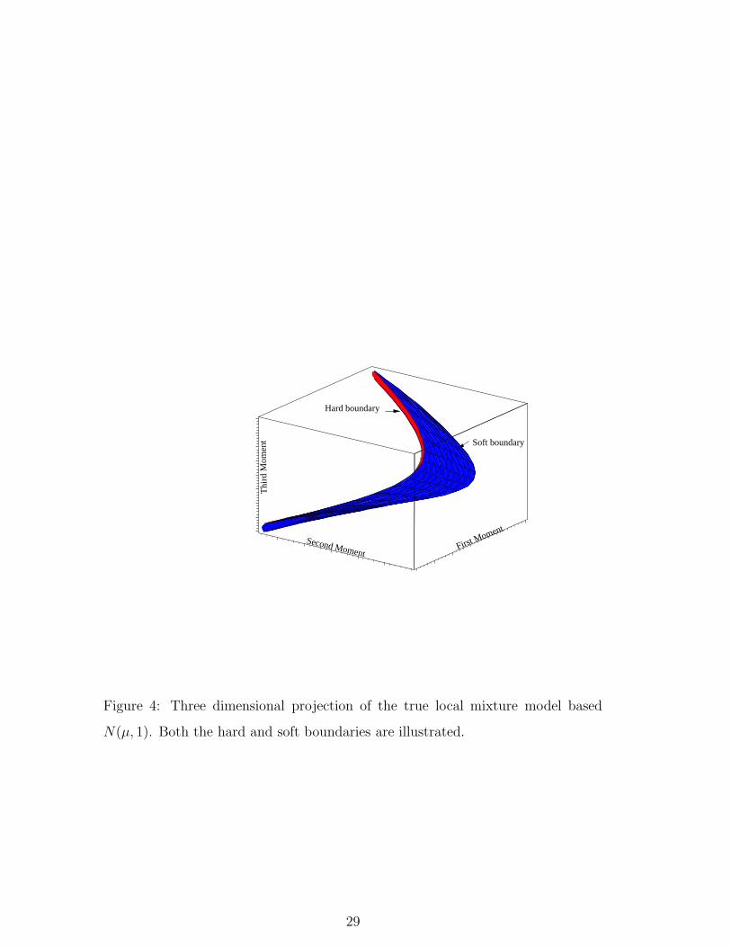
Soft boundary

Hard boundary

Thi

rd M

omen

t

First Moment

Second Moment

Figure 4: Three dimensional projection of the true local mixture model based

N(µ, 1). Both the hard and soft boundaries are illustrated.

29

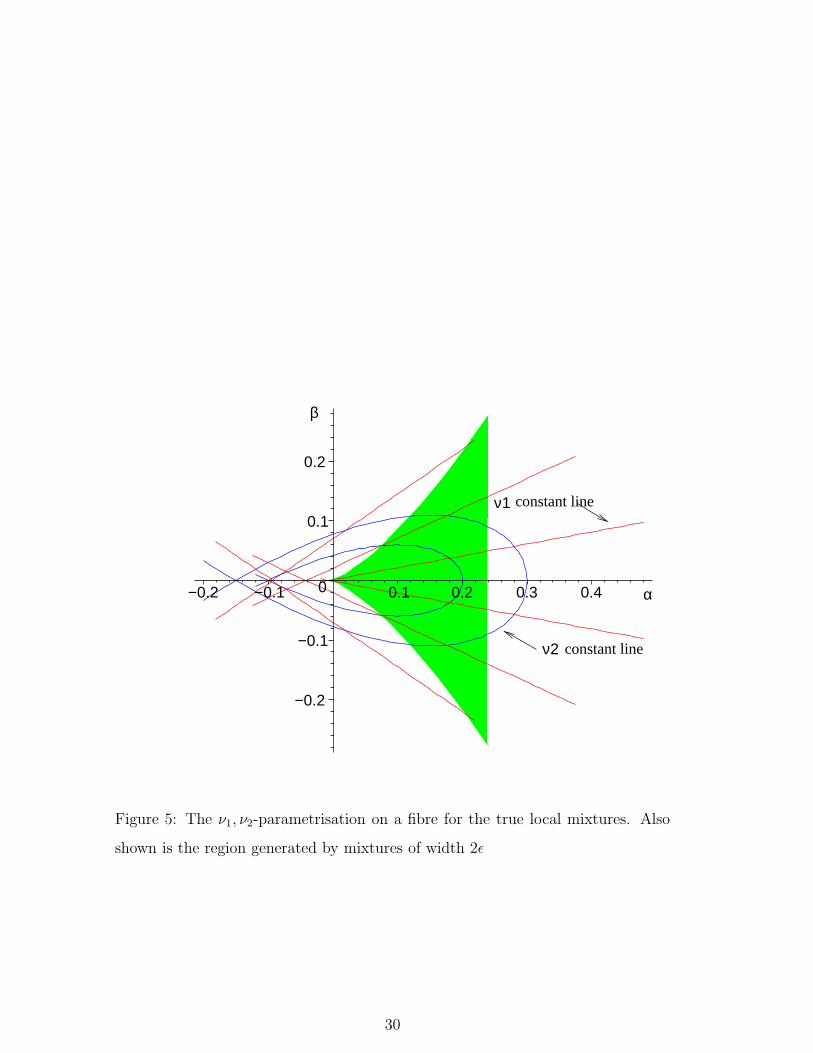
ν1

ν2

constant line

� � � � � � � � ��

� � � � � � � � ��

constant line

−0.2

−0.1

0

0.1

0.2

−0.2 −0.1 0.1 0.2 0.3 0.4 α

β

Figure 5: The ν1, ν2-parametrisation on a fibre for the true local mixtures. Also

shown is the region generated by mixtures of width 2ε

30

0.0 0.5 1.0 1.5 2.0

−13

0−

120

−11

0−

100

rho

log−

lik

Figure 6: The log-likelihhood for a simple mixture.

31

(a) Log likelihood contours

nu1

nu2

−2.0 −1.0 0.0 0.5 1.0 1.5

−0.

50.

00.

51.

0

(b) Log likelihood contours

α

β

Hard

Hardboundary

Soft boundary

boundary

0.0 0.2 0.4 0.6 0.8 1.0 1.2

−1.

00.

00.

51.

01.

5

(c) Posterior of alpha

α

Den

sity

0.0 0.5 1.0 1.5

0.0

0.5

1.0

1.5

(d) Posterior of beta

Den

sity

−1.0 −0.5 0.0 0.5 1.0 1.5

0.0

0.2

0.4

0.6

0.8

1.0

β

Figure 7: (a) Log likelihood contours in ν1, ν2-parameters for orthogonal slice of

local mixture models. (b) Log likelihood contours in α, β-parameters for orthogonal

slice of true local mixture models. (c) posterior distribution for α (d) posterior

distribution for β 32

(a) The data

data

Fre

quen

cy

0 2 4 6 8 10

05

1015

(b) Posterior for mu

mu

Den

sity

3.0 3.5 4.0 4.5

0.0

0.5

1.0

1.5

(c) Posterior for alpha

alpha

Den

sity

0.0 0.5 1.0 1.5

0.0

0.5

1.0

1.5

(d) Posterior for beta

beta

Den

sity

−0.5 0.0 0.5 1.0 1.5 2.0

0.0

0.2

0.4

0.6

0.8

1.0

Figure 8: (a) The data (b) The posterior distribution for µ with the vertical line

showing the value of the sample mean (c) the posterior distribution for α (d) the

posterior distribution for β

33

(a) data

skewdata

Fre

quen

cy

2 4 6 8 10 12

05

1015

2025

0.0 1.0 2.0 3.0

−0.

50.

00.

51.

01.

52.

02.

53.

0

(b) Sample of alpha, beta

Alpha

Bet

a

+++++++++

+++++++++++++++++++++++

++

+++++++

+

++

++

++ +++

++++++++++++++++

+ +++++++++++

+++

+

+++++++++++++ +++

+

++

+++++

++++

+++++ +++ +

++

++

+++++++++++ ++++++++ ++

++++++++++++

++

+

+++ ++++

++++++++++

+

+++

++++ +

++++++++

++++ +++

++++++++ ++++++++

++++

++

+++

++++ +++++++++ ++++++++ +

++++++

+

++++++

++++++++

+++++++++

++++++++++++++

+++++++ +

++

++++

+++++

+

++ ++ ++++++ ++++

+++++++

+

+

+++++

++++++

+ +++++

++++

+ +

++

+++

+++++++++++++

++

++ +++++++++++

++

++++++++++++

+++ +++++++

++++++

+++++ ++

++

+

++++++++++

+++++++++

++++++++ +++++++++

+++++ +++++++

++

++++++ ++

++++++

+++

+++++

+++

++++++++

++++++++ +++++ +

++++

++++

++ ++++

++++

++++++++++

+++++ ++ +++++

++++++++

+++ ++ +++++++++++++

++++++

++++

++

+++

++++

++

++++

+++

+++++++ +++

+++++

++

+++

++++++++++++

++++

+

+

+++++

+++

+++ ++++++++

++++++

+

++++++++++++

+++

++

+

+++

+++++++

++++

+++

++++++

++++

++++++

+++

+ ++

++++

+++++++ + +++ +++++++

+ ++++++

+++++++

+ +++

+++++++++++++++++

++

++

+++++ +++++ ++

++ ++++

++

++++

+++++

++++

++++++ ++++

4.0 5.0 6.0 7.0

0.0

0.5

1.0

1.5

(c) Posterior for mu

N = 847 Bandwidth = 0.1946

Den

sity

Figure 9: (a) The data (b) The Markov chain Monte Carlo sample for α and β.

In the unrestricted case the points are illustrated with dots, in the restricted case

with crosses. (c) Density estimates for the the posterior distributions for µ, solid

line unrestricted case, dash line restricted case.

34

Documents

Local Mixtures and Exponential Dispersion Models