Embed Size (px)
Citation preview

Local Mispricing and Microstructural Noise:
A Parametric Perspective∗
Torben G. Andersen† Ilya Archakov‡
Gokhan Cebiroglu§ Nikolaus Hautsch¶
This Version: October 2019
Abstract
We extend the classic ”martingale-plus-noise” model for high-frequency returns to accom-
modate an error correction mechanism and endogenous pricing errors. It is motivated by (i)
novel empirical evidence documenting that microstructure noise is interwoven with innova-
tions to the efficient price; (ii) building a bridge between high-frequency econometrics and
market microstructure models. We identify temporal pricing error corrections and noise
endogeneity as complementary components driving high-frequency dynamics and inducing
two separate regimes, characterized by the sign of the return serial correlation and an im-
plied bias in realized variance estimates. We document frequent fluctuations between these
regimes, which we associate with price discovery in a setting with incomplete information
and learning. The model links critical concepts from high-frequency statistics and market
microstructure theory, opening up new paths for volatility estimation.
Keywords: volatility estimation; market microstructure noise; price reversal; momentum;
contrarian trading; JEL classification: C58, C32, G14
∗We thank participants of the ”Jan Mossin Symposium,” Bergen, 2016; FERM, Guangzhou, 2016; SoFiE,
Aarhus, 2016; ”New Developments in Measuring and Forecasting Financial Volatility,” Durham, NC, 2016; MFA
Meeting, Chicago, 2017; Stevanovich Conference, University of Chicago, 2018; IAAE Conference, Nicosia, 2019;
and seminars at Aarhus University, Humboldt University, Universitat Pompeu Fabra, UNC at Chapel Hill, Vienna
University of Economics and Business, the U.S. Commodity Futures Trading Commission, and the University of
Giessen for comments and discussions. We are grateful to Peter R. Hansen for valuable comments. Andersen
acknowledges support from CREATES (DNRF78), funded by the Danish National Research Foundation. Hautsch
acknowledges financial support from the Wiener Wissenschafts-, Forschungs- und Technologiefonds (WWTF).†Kellogg School of Management, Northwestern University and NBER. Email: [email protected].‡Department of Statistics and Operations Research, University of Vienna. Email: [email protected].§Credit Suisse, London. Email: [email protected]. The views, thoughts, and opinions expressed in this
article belong solely to the author, and are not necessarily shared by the author’s employer.¶Department of Statistics and Operations Research, and the Research Platform ”Data Science @ Uni Vi-
enna,” University of Vienna, Vienna Graduate School of Finance and Center for Financial Studies. Email: niko-

1 Introduction
The increasing availability of high-frequency asset price data has spurred two largely separate
literatures. One focuses on model-free ex-post measurement of features concerning the realized
return path, with the main attribute of interest being the realized volatility, representing the
empirical quadratic return variation. The premise is that asset prices reflect an underlying
arbitrage-free “efficient” or “fundamental” return process polluted by microstructure noise
(MMN), due to rounding to a price grid, varying transaction and quote intensities, private
information, bid-ask spreads, and other trading costs. Hence, the fundamental log-price process
is a semimartingale, while MMN is viewed as a nuisance factor. Implicitly, this literature
presumes that all relevant information is impounded instantaneously so that, at all times,
transaction prices and quotes embed the latent efficient equilibrium price, bracketed by the bid-
ask spread. Consequently, at the micro level, the fundamental price is “hidden” through a MMN
distortion which, locally, are of non-trivial order. As a result, much work has been devoted
to MMN-robust inference for realized components of the efficient price process, see, e.g., the
classic articles in Andersen and Bollerslev (2018b), the survey by Andersen and Bollerslev
(2018a), and the book treatment of Ait-Sahalia and Jacod (2014).
Whereas the realized volatility literature generally treats the fundamental price innovations
as exogenous, a central topic in the market microstructure literature is price discovery. This
literature explores a variety of complications, including asymmetric information, heterogeneous
trading motives, and market design features. Here, learning, price impact, and strategic trading
arise as natural phenomena. The interaction of such features generates a complex environment,
so most theoretical microstructure models are fairly stylized, allowing for specific aspects of the
price discovery process to be explored in isolation. For example, Kyle (1985) analyzes strategic
trading of a risk-neutral agent with monopolistic private information, finding information to be
incorporated into the price slowly, as the informed agent spreads trades over time to manage
price impact. In contrast, Holden and Subrahmanyam (1992) show that information revelation
occurs rapidly if there are multiple informed agents. Likewise, both information acquisition
and risk aversion can have similar effects, see, e.g., Holden and Subrahmanyam (1996). Vives
(1995) also demonstrates that the speed of information revelation is negatively correlated with
the degree of risk aversion among informed agents and the amount of noise trading. Finally, in a
stylized setting, Glosten and Milgrom (1985) show that the bid (ask) prices represent conditional
expectations of the efficient price conditional on a sell (buy) transaction, so the “noise” in the
realized volatility literature is literally intertwined with innovations to the fundamental price.
In summary, typical microstructure models imply that noise is endogenous because inno-
vations to the transaction prices and quotes interact with the efficient price process through
1

learning and temporal feedback mechanisms. At the same time, microstructure theory is largely
void of the return dynamics of primary interest in the econometric work focusing on realized
volatility. In this paper, we build bridges between these strands of the literature. In particular,
as a methodological contribution, we suggest estimating the fundamental volatility over short
intraday windows from our microstructure model in a manner that corrects realized volatility
measures for MMN effects. By cumulating the former estimators, we obtain an alternative return
variation measure that generally is consistent with the RV measures, but deviates systematically
under specific market conditions, reflecting the relative strength of different MMN distortions.
As an initial step, we document, empirically, the presence of persistent time-varying return
autocorrelation, inconsistent with a noise process that is orthogonal to the fundamental price.
At the same time, the return correlation pattern displays pronounced fluctuations. As a vivid
illustration, Figure 1 provides volatility signature plots for four different stocks on selected days.
The upward sloping curves (as one approaches the origin) in the left panels are similar to the
biases induced by i.i.d. noise, which generate an MA(1) structure and negative return serial
correlation, as noted by Roll (1984).1 However, our sample of Nasdaq stocks contains many
examples of the exact opposite behavior. This is exemplified by the right panels, where the
signatures drop sharply as we approach the highest sampling frequencies, reflecting pronounced
positive serial correlation. Consistent with such findings, studies–going back at least as far as
Hansen and Lunde (2006)–show that the high-frequency return dynamics is inconsistent with
an MA(1) representation, as also touched on by Hasbrouck and Ho (1987). In-and-of-itself,
positive serial dependence may be rationalized by a more general specification of the noise
process. However, if noise is uncorrelated with the efficient price, it will only augment the
overall return variation, implying that signature plots will be increasing at high frequencies,
where the noise is dominant. That is, a declining return variation at high frequencies is only
feasible, if the noise and fundamental return innovations are (negatively) correlated, i.e., the
noise is endogenous. Hence, such MMN features leave a distinct footprint in the data.
The above evidence points towards time-varying return dependencies that are at odds with
the semimartingale paradigm and are not readily accommodated through the infill asymptotic
inference procedures commonplace within the high-frequency econometrics literature. More-
over, the presence of endogenous noise raises fundamental questions regarding our ability to
separately identify the return volatility associated with the efficient price versus noise innova-
tions. These considerations lead us to adapt a simple discrete-time parametric framework that
allows for rapidly shifting regimes, yet also provides a tractable and economically interpretable
setting, highlighting the impact of microstructural traits on the high-frequency dynamics.
1In a fully parametric setting, this property can be exploited to construct estimators of both the “fundamental” andMMN variance, see, e.g., Zhang et al. (2005).
2

Figure 1: The figure depicts signature plots for the Realized Variances (RV) computed for 4 stocks (Facebook,Apple, Ebay and Amazon) on selected trading days. The left and right panels illustrate cases with downwardand upward sloping signature plots, respectively. For each sampling frequency ∆ (from 1sec to 120sec with aone-second step), we compute the RV measure for multiple ”grids” obtained by shifting the initial price observationup by one second to ∆ seconds (thus, for ∆=1sec we have one grid and for ∆=120sec, we obtain 120 grids).Blue dots correspond to daily RV estimates computed from different underlying sampling frequencies and all gridconfigurations. The red solid lines represent the average values of RV across all grids (the so-called sub-sampledRV).
To ensure a transparent setup, we extend the classic ”martingale-plus-noise” model by
components accommodating an error correction mechanism and price endogeneity. These
features arise naturally once one recognizes that the investors’ information set is imperfect
and subject to acquisition and processing delays. Under these circumstances, investors cannot
determine, with certainty, whether a given price increase is due to the arrival of positive (private)
news or random net buying orders from liquidity traders (noise). In the former case, the price is
likely to continue its upward trajectory while, in the second case, the price tends to revert to its
prior level. Even if astute traders avoid systematic mispricing, the valuation is only unbiased
on average. During episodes with sustained imbalances in net liquidity demand or an unusual
intensity of privately informed trading, rational agents tend to err in their instantaneous valuation
in the same direction. At the same time, rationality does imply that simple momentum and
contrarian strategies cannot earn significant profits. The fact that we find positive and negative
3

return autocorrelation patterns about equally common is consistent with the latter hypothesis.
The ingredients of our model are not new to the MMN literature, but no existing tractable
framework simultaneously accommodates noise endogeneity and pronounced variation in the
return autocorrelation pattern. We retain tractability by stipulating that our model applies only
locally, and thus allow the model parameters to vary across intraday intervals. This flexible
approach is aligned with our empirical evidence, showing that momentum and contrarian
regimes, and thus the sign of return autocorrelations, may alternate frequently across the trading
day. It effectively allows the shifting market environment to guide the evolution of the system.
Moreover, the use of a local approximating model with constant volatility enables us to sidestep
the difficult task of jointly modeling the intraday patterns and the persistent activity dynamics.
Our model mimics features associated with learning via an error correction mechanism,
reminiscent of the partial adjustment dynamics introduced by Amihud and Mendelson (1987). It
includes four parameters; (i) the volatility of the random walk process (“fundamental volatility”);
(ii) the “magnitude of the noise,” or noise-to-signal ratio; (iii) the speed of reversal from
mispricing, which is closely related to the persistent autocorrelation or momentum effects; and
(iv) the instantaneous response to efficient price innovations, capturing the extent of mispricing
due to informational frictions. These parameters allow for both dynamic error correction
and price endogeneity features with differential implications for the return autocorrelation
pattern. Furthermore, the specification enables us to separate these components and render them
statistically identifiable and economically interpretable.
This parsimonious representation captures various return dependencies implied by existing
microstructure models. In particular, the classical “martingale-plus-noise” model as well as
variants, allowing the noise to be correlated with the efficient returns, emerge as special cases.
Combined with our ability to accommodate heterogeneity across intraday intervals, we obtain
a setting reminiscent of the endogenous noise representation analyzed by Kalnina and Linton
(2008).2 Our approach is also related to prior studies that link the properties of noise more
explicitly to the process of trading and the underlying microstructure, see, e.g., Madhavan et al.
(1997), Diebold and Strasser (2013), Chaker (2013) and Li et al. (2016). However, none of these
studies consider the type of high-frequency variation in the mispricing and temporal feedback
effects that we deem crucial in explaining the return dynamics observed in Figure 1.
In our model, the speed of price reversion interacts with the noise-to-signal ratio to determine
the sign of the return autocorrelation. We classify the market environment accordingly as
belonging to one of two regimes. In one, the impact of “mispricing” is dominated by the
strength of the price reversal, induced by idiosyncratic noise shocks, so the returns display
negative serial correlation, or “contrarian” traits. In the other regime, the feedback from
2See also Sheppard (2013) for a related notion intended to measure market “speed.”
4

mispricing generates “momentum,” or positive return autocorrelation.
The irregular alternation between such return dependency regimes have important implica-
tions for standard volatility measures based on high-frequency returns, see, e.g., Andersen et al.
(2003). In the contrarian regime, realized volatility tends to exaggerate the quadratic variation
of the efficient price, inducing the well-known upward-shaped volatility signature plots. In
the other regime, high-frequency sampling causes downward-shaped signature plots. Even
more fundamentally, prolonged periods of nontrivial return autocorrelation renders the standard
infill asymptotic approach problematic, because the associated finite-sample approximations
assume that the return dependencies are negligible beyond short (calendar) time windows. The
latter assumption, however, is not compatible with market microstructure approaches featuring
learning and pricing error corrections, as such mechanisms make return dependencies persist for
extended periods and are naturally cast in discrete time. In fact, the difficulty to align temporal
feedback effects in market microstructure models with infill asymptotics, where pricing errors
(in the limit) should be corrected instantaneously, is one of the major reasons why there is no
straightforward connection between common approaches for high-frequency based volatility
estimation and market microstructure models. For these reasons, we turn towards a discrete-time
representation and employ more traditional methods of inference.
Conveniently, our model may be cast in a linear state-space form, enabling estimation via
the Kalman filter. This facilitates consistent estimation of the (locally constant) volatility, albeit
with non-negligible error for short horizons. The setting encompasses several alternative models,
including the i.i.d. martingale-plus-noise and Amihud and Mendelson (1987) specifications,
allowing us to test their relative merits. In addition, we analyze identification issues arising from
mispricing and noise endogeneity. We find that the fundamental return volatility is identified,
even if the signal-to-noise ratio and the degree of noise endogeneity are only partially identified.
As such, our approach represents a step towards the development of high-frequency volatility
estimators that retain a link to the existing market microstructure literature and allow for a more
structural treatment of the impact due to noise shocks.
We estimate the model over intraday intervals using mid-quote returns sampled at different
frequencies. The analysis points towards a high degree of informational efficiency, although
the price discovery process also involves a non-trivial element of sluggishness. We identify
strong intraday periodicities in the speed of price discovery and, strikingly, find that fundamental
volatility is highly elevated at the market open and flat through the remainder of the trading day.
The dramatic increase in market activity towards the market close is, in contrast, driven by a spike
in uninformed trading and idiosyncratic noise. This illustrates the potential of our approach
to build a foundation for new quantitative measures of market efficiency and fundamental
volatility. Formal econometric tests favor our flexible parameter approach, involving a lagged
5

price adjustment mechanism, relative to popular stylized microstructure models.
The rest of the paper is structured as follows. Section 2 provides comprehensive evidence
for locally significant return autocorrelation of varying sign. Section 3 introduces the model,
explores its dynamic properties, and its relation to existing models. Section 4 focuses on
identification issues in our general specification and reviews our estimation strategy. Section
5 present our detailed empirical findings, and Section 6 concludes. Auxiliary materials are
deferred to a Supplementary Appendix, including also a large-scale Monte Carlo study.
2 Local Regimes of Significant Return Autocorrelation
This section provides novel empirical evidence for the existence of short-lived regimes, charac-
terized by distinct levels of return autocorrelation. That is, the return series vacillates between
periods with significantly positive, insignificant, and significantly negative return dependence.
We quantify the return serial dependence over consecutive short intervals using high-frequency
mid-quote prices of the Nasdaq 100 equity index constituents, obtained from LOBSTER.3 To
keep the analysis manageable, we restrict our sample to the first three months of 2014 yielding
a total of 61 trading days. For each day, we consider the full 6.5 hour trading period.
Since we focus on the properties of mid-quote returns across short intervals, spanning 10-20
minutes, we split our sample into quintiles based on the average daily number of mid-quote
revisions, with Group 1 being the 20% of stocks with most frequent revisions and Group 5 being
the 20% with the fewest. While we concentrate our discussion on the most liquid groups, we
convey a sense of robustness by reporting results for the full spectrum of stocks.
Figure 2 displays the distribution of daily mid-quote revisions, with the vertical lines
providing the partitioning into five liquidity groupings. The corresponding quintiles amount
to 17,485, 10,365, 8,166, 5,531 and 2,497 average daily mid-quote revisions, respectively. If
we sample every 5 seconds (over 6.5 hours of trading), we have 4,680 return observations per
day. Consequently, for a typical stock in Group 5, we usually have fewer quote revisions than
intra-day returns, whereas this ratio is much more favorable for stocks in Groups 1 to 4.
2.1 Significance of Return Autocorrelations in Local Intervals
We face the challenge of identifying return autocorrelations over local intervals of unknown (and
possibly) time-varying lengths. If individual stocks truly do undergo alternating periods with
different degrees of return autocorrelation – ranging from significantly negative to significantly
positive – but such episodes are fairly short, of varying duration and not directly observed, we
3The LOBSTER database (https://lobsterdata.com) builds on Nasdaq’s historical TotalView-ITCH data. It providesinformation on all trade and quote activity on Nasdaq at nano-second time stamp precision.
6

5000 15000 25000 35000 45000Average mid-quote updates (per day)
0
2
4
6
8
10
12
14
Stoc
ks from
the sa
mple
Figure 2: Empirical distribution of per-stock averages of daily mid-quote revisions for 100 considered Nasdaqstocks, based on the first 61 trading days in 2014. The vertical dashed lines corresponds to the 20th, 40th, 60th and80th percentiles of the empirical distribution, thus partitioning the sample into five corresponding liquidity groups.
need to adopt a methodology designed to detect this type of deviation from the null hypothesis of
constant return autocorrelation. On the one hand, autocorrelations computed over long intervals
provide limited power against local fluctuations in the sign and size of serial correlations, as the
values are averaged across short-lived within-period regimes, implying that the autocorrelation
statistics are biased towards zero. On the other hand, we require a non-trivial number of return
observations to obtain statistics with reasonable precision, suggesting the use of longer intervals.
To address this bias-variance trade-off, we employ different test procedures and robustify our
results by analyzing local intervals of different lengths (10, 15, and 20 minutes) and sampling at
different, but relatively high frequencies, ∆ = 2, 3, and 5 seconds, guaranteeing a fairly large
number of observations within each interval. For the most illiquid stocks, this is an aggressive
choice, and we may expect the findings for Group 5 to reflect the impact of microstructure
effects and, especially, irregular trading.
Invoking the null hypothesis of zero return autocorrelation, it is natural to initially test
whether an abnormal number of intervals generates excessively high absolute serial correlation.
To formalize the procedure, denote the intra-day mid-quote log-return for a given stock over
interval i by ri, with i ranging across an equidistant grid i = 1, . . . ,M . Throughout the paper,
we assume that the drift (unconditional mean) over short (intraday) intervals are negligible,
imposing E[ri] = 0. We then split the intra-daily trading period into Kd local intervals (ranging
from 10 to 20 minutes), with N = bM/Kdc observations in each interval. For a sample with D
trading days, we have a total of K = DKd local intervals in our sample. For k = 1, . . . ,K, the
empirical (first-order) autocorrelation for interval k is ρk =(∑N−1
i=1 ri,kri−1,k
)/∑N
i=1 r2i,k,
7

where ri,k denotes the i-th midquote return in interval k.4
For inference robust to heteroskedasticity and volatility clustering in high-frequency returns,
stemming from stochastic volatility and intraday periodicity effects, we apply asymptotic limit
results by Kokoszka and Politis (2011). Under mild assumptions on the return moments and the
dependence in the squared return process, they demonstrate that,
√N (ρk − ρk)
d→ N (0, Vk) ,
where the asymptotic variance Vk can be consistently estimated by
Vk =(N − 1)−1
∑N−1i=1 r2
i,kr2i−1,k
(N−1∑N
i=1 r2i,k)
2.
Under the null hypothesis H0 : ρk = 0, for all k, the local estimates ρk are noisy estimates
of zero, stemming from asymptotically independent, non-identical Gaussian distributions. To
gain power, we do not aim at testing the significance of local autocorrelations for each individual
interval, but focus on averages of absolute (local) autocorrelations. Given the results above, the
absolute autocorrelations |ρk| are asymptotically distributed as a half-normal random variate
with E[|ρk|] =√
2Vk/(Nπ) and V[|ρk|] = (1 − 2/π)Vk/N for all k. Then, by a standard
central limit theorem, under H0, the average absolute autocorrelation ρ = K−1∑
k |ρk|,asymptotically follows the distribution,
ρa∼ N
(1
K
∑k
√2VkNπ
,1
K2N
(1− 2
π
)∑k
Vk
). (1)
Hence, by constructing a test for ρ using the quantiles associated with the distribution in
equation (1), we obtain a test with power against the alternative of local autocorrelations of
varying signs. To test separately for positive and negative autocorrelations, we split the sample
of K intervals into the subsamples I− and I+, consisting of intervals where ρk is positive
or negative, respectively. Accordingly, one-sided average absolute autocorrelations are given
by ρ+ = K−1+
∑k∈I+ |ρk| and ρ− = K−1
−∑
k∈I− |ρk|, respectively, where K+ = |I+| and
K− = |I−|. The asymptotic distributions of ρ+ and ρ− are readily derived as for ρ above.
Hence, this test has power to separate average empirical autocorrelation estimates of a given
sign from random realizations of the same sign generated by the null distribution.
Table 1 reports the corresponding test results. The choice of T and ∆ trades off estimation
efficiency (increasing for low ∆ and large T ), biases due to the possible impact of market
4In unreported results, we find qualitatively similar autocorrelation results for the corresponding transaction returns.
8

T = 10 min T = 15 min T = 20 min
(I) (I+) (I−) (I) (I+) (I−) (I) (I+) (I−)
∆ #5%#1%#5%#1%#5%#1% π+ #5%#1%#5%#1%#5%#1% π+ #5%#1%#5%#1%#5%#1% π+
Liquidity group 1 (20 most liquid assets from NASDAQ 100)
2 sec 20 20 20 20 14 13 0.57 20 20 20 20 14 12 0.58 20 20 20 20 14 12 0.593 sec 20 20 20 20 11 10 0.58 20 20 20 20 12 10 0.59 20 20 20 20 12 9 0.605 sec 20 20 20 20 11 9 0.59 20 20 20 20 11 10 0.60 20 20 19 19 10 9 0.62
Liquidity group 2
2 sec 20 20 20 20 17 17 0.53 20 20 20 19 17 17 0.54 20 20 20 20 17 16 0.543 sec 20 20 20 20 16 15 0.55 20 20 20 20 15 14 0.55 20 20 20 20 15 15 0.565 sec 20 20 20 20 15 12 0.57 20 20 20 20 14 11 0.58 20 20 20 20 11 10 0.59
Liquidity group 3
2 sec 20 20 18 18 20 19 0.49 20 20 18 18 18 18 0.49 20 20 18 18 18 16 0.503 sec 20 20 18 18 20 15 0.52 20 20 18 18 18 16 0.52 20 20 18 18 14 11 0.535 sec 20 20 19 19 16 12 0.55 20 20 18 18 14 10 0.56 20 20 18 18 9 7 0.57
Liquidity group 4
2 sec 20 20 18 18 20 19 0.44 20 20 18 17 19 19 0.45 20 20 18 15 19 19 0.453 sec 20 20 18 17 20 19 0.48 20 20 18 17 18 18 0.48 20 20 17 17 18 17 0.485 sec 20 20 19 19 17 17 0.51 20 20 19 18 16 16 0.52 20 20 20 19 17 14 0.53
Liquidity group 5 (20 least liquid assets from NASDAQ 100)
2 sec 20 20 19 14 20 19 0.27 20 20 14 10 20 19 0.30 20 20 11 8 20 19 0.313 sec 20 20 18 15 20 20 0.29 20 20 14 11 20 20 0.32 20 20 11 10 20 19 0.335 sec 20 20 18 14 20 19 0.32 20 20 17 11 20 19 0.35 20 20 14 7 20 18 0.36
K = 2379 K = 1586 K = 1159
Table 1: Significance of first order return autocorrelations calculated for local intra-daily intervals of length T =10, 15, and 20 minutes. Columns #5% and #1% report the number of stocks (out of 20 in each liquidity group) forwhich the null hypothesis is rejected at 5% and 1% significance level, respectively. Columns marked by (I) referto the results of the test which is based on all intervals in the sample, while columns under (I+) and (I−) refer toresults based on intervals with only positive or only negative autocorrelations, respectively. Columns π+ provide theaverage (across stocks) fraction of intervals with positive return autocorrelations over the full sample of K intra-dailyintervals (K is reported in the bottom of the table). The tests are conducted for local intervals observed during 61consecutive trading days spanning the first three month of 2014. Results are reported separately for five groups ofstocks sorted by the average number of daily mid-quote revisions.
microstructure noise (worsens for small ∆) and the superposition of local autocorrelation
regimes (problematic for large T ) versus the resulting power of the test. We report inference
based on local intervals of T = 10, 15, and 20 minutes, computed at sampling frequencies ∆ =
2, 3, and 5 seconds. The results are based on the first 61 trading days of 2014 and are reported
separately for stocks from the five liquidity groups defined above.
We report on the test for absolute autocorrelation ρ in the columns marked by (I), while
those marked (I+) and (I−) concern ρk for k ∈ I+ and k ∈ I−, respectively. We indicate the
number of stocks (out of 20 in each liquidity class) for which we reject the null at 1% and 5%
confidence levels, together with the relative proportions of intervals belonging to I+ (or I−).
First, for every single stock, we reject the null hypothesis of constant first-order return
9
autocorrelation of zero. For a vast majority of stocks, we also reject the null for most configura-
tions of T and ∆, when positive and negative autocorrelations are considered separately. The
fraction of intervals with positive serial correlation ranges between 27% and 62%, depending on
the liquidity group, sampling frequency ∆ and interval length T . Hence, the evidence clearly
supports the hypothesis of significant local return serial correlation of varying signs.
Secondly, for most liquid stocks (group 1 and 2), we reject the null more often for regimes
of positive than negative autocorrelation. This pattern reverses for the low-liquidity groups 4
and 5, revealing asymmetries with respect to the intensity of the quote revisions. For longer
intervals, T , rejections of the null are slightly less frequent, likely due to a loss of power caused
by variations in the return dynamics within the intervals. Conversely, the proportion of rejections
is largely independent of the sampling frequency, ∆.
Finally, we generally observe more intervals with positive than negative autocorrelations
(K+ > K−) for the stocks from the first three liquidity groups. This suggests that a form of
“momentum” is a major driver of the local return dependence structure.
2.2 Persistence of Return Autocorrelations
We now explore the persistence of the regimes. Predictability of the sign of the return autocorre-
lation across local windows is inconsistent with the hypothesis of zero return dependencies and
suggests the existence of local regimes with shifting autocorrelation structures.
By defining the indicator variable
θk = 1{ρk≥0
}, k = 1, . . . ,Km
we apply a standard nonparametric Wald–Wolfowitz runs test to assess whether θk is purely
random. A ”run” is defined as a string of identical elements in the indicator sequence. Assuming
independent elements, the number of runs, Rθ, follows the asymptotic distribution,
Rθ ∼ N
(2π+π−K + 1, 4π2
+π2−K
2 − 2π+π−K
K − 1
),
where π+ = 1K
∑k θk = K+/K and π− = 1−π+ = K−/K denote the proportions of positive
and negative autocorrelation regimes, respectively. Table 2 reports results for different choices
of T and ∆. The null is rejected for a clear majority of stocks, even at the 99% confidence level.
Moreover, the rejections fall consistently in the left tail, indicating (positive) persistence.
To explore the underlying dependence structure, we implement a test based on the serial
correlation in the local return autocorrelation regime. We define {θk} as a homogeneous Markov
chain of order one with transition probability pij = Prob(θk+1 = j∣∣θk = i), with i, j ∈ {0, 1}.
10

T = 10 min T = 15 min T = 20 min∆ #2.5 #97.5 #0.5 #99.5 π+ #2.5 #97.5 #0.5 #99.5 π+ #2.5 #97.5 #0.5 #99.5 π+
Liquidity group 1 (20 most liquid assets from NASDAQ 100)
2 sec 19 0 19 0 0.57 19 0 17 0 0.58 19 0 17 0 0.593 sec 19 0 18 0 0.58 20 0 18 0 0.59 19 0 17 0 0.605 sec 20 0 17 0 0.59 19 0 18 0 0.60 19 0 15 0 0.62
Liquidity group 2
2 sec 20 0 20 0 0.53 18 0 16 0 0.54 14 0 14 0 0.543 sec 18 0 18 0 0.55 17 0 14 0 0.55 19 0 16 0 0.565 sec 19 0 17 0 0.57 19 0 18 0 0.58 17 0 17 0 0.59
Liquidity group 3
2 sec 17 0 14 0 0.49 17 0 14 0 0.49 15 0 11 0 0.503 sec 15 0 15 0 0.52 18 0 16 0 0.52 18 0 15 0 0.535 sec 16 0 15 0 0.55 18 0 16 0 0.56 16 0 14 0 0.57
Liquidity group 4
2 sec 20 0 14 0 0.44 16 0 14 0 0.45 13 0 12 0 0.453 sec 19 0 16 0 0.48 15 0 12 0 0.48 17 0 12 0 0.485 sec 18 0 17 0 0.51 16 0 13 0 0.52 16 0 11 0 0.53
Liquidity group 5 (20 least liquid assets from NASDAQ 100)
2 sec 18 0 15 0 0.27 15 0 13 0 0.30 16 0 12 0 0.313 sec 19 0 17 0 0.29 17 0 13 0 0.32 15 0 10 0 0.335 sec 18 0 15 0 0.32 17 0 10 0 0.35 14 0 11 0 0.36
K = 2379 K = 1586 K = 1159
Table 2: The table reports on Wald–Wolfowitz run tests for intervals of T = 10, 15, and 20 minutes. The nullhypothesis asserts that positive vs. negative return autocorrelation regimes follow an independent random sequence.The number of stocks (out of 20), for which we reject the null, are given in columns labeled %2.5, %0.5 (left tailrejections) and %97.5, %99.5 (right tail rejections). Columns π+ provide the average (across stocks) fraction ofintervals with positive return autocorrelation in the full sample of K intraday intervals. The sample covers 61 tradingdays spanning the first three month of 2014. Results are reported separately for stocks sorted by the intensity ofmid-quote revisions, with the highest in Group 1 and the lowest in Group 5.
The null hypothesis stipulates that θk is an i.i.d. Bernoulli process, i.e., p00 = p10 = p and
p01 = p11 = 1− p, so θk should be Bernoulli distributed with E[θk] = p and V[θk] = p(1− p),
∀k. A natural estimator for pij , pij , is the proportion of transitions from state i to state j relative
to the total number of observations for state i. Under the null, letting π+ denote the sample
estimate of p and K →∞, pij is asymptotically distributed as
pij ∼ N
(1{
i=1}(2π+ − 1) + π−,
π+π−K
).
Table 3 reports results for different values of T and ∆. The null hypothesis of random
variation in the sign of the autocorrelation is rejected in most cases. Notably, the rejections are
associated exclusively with extreme right tail realizations of the test statistic, indicating that both
positive and negative autocorrelation regimes display persistence across adjacent local intervals.
11

Persistence of positive regimes (H0: p11 = p) Persistence of negative regimes (H0: p00 = 1− p)
10 min 15 min 20 min 10 min 15 min 20 min∆ #2.5 #97.5 π+ #2.5 #97.5 π+ #2.5 #97.5 π+ #2.5 #97.5 π− #2.5 #97.5 π− #2.5 #97.5 π−
Liquidity group 1 (20 most liquid assets from NASDAQ 100)
2 sec 0 20 0.57 0 19 0.58 0 16 0.59 0 19 0.43 0 19 0.42 0 19 0.413 sec 0 18 0.58 0 18 0.59 0 17 0.60 0 19 0.42 0 20 0.41 0 18 0.405 sec 0 18 0.59 0 18 0.60 0 15 0.62 0 20 0.41 0 20 0.40 0 19 0.38
Liquidity group 2
2 sec 0 20 0.53 0 17 0.54 0 13 0.54 0 20 0.47 0 18 0.46 0 16 0.463 sec 0 18 0.55 0 14 0.55 0 16 0.56 0 18 0.45 0 19 0.45 0 20 0.445 sec 0 18 0.57 0 18 0.58 0 15 0.59 0 20 0.43 0 19 0.42 0 17 0.41
Liquidity group 3
2 sec 0 16 0.49 0 17 0.49 0 14 0.50 0 15 0.51 0 17 0.51 0 14 0.503 sec 0 16 0.52 0 17 0.52 0 18 0.53 0 15 0.48 0 18 0.48 0 16 0.475 sec 0 16 0.55 0 17 0.56 0 15 0.57 0 16 0.45 0 17 0.44 0 17 0.43
Liquidity group 4
2 sec 0 20 0.44 0 16 0.45 0 15 0.45 0 15 0.56 0 15 0.55 0 13 0.553 sec 0 17 0.48 0 15 0.48 0 16 0.48 0 18 0.52 0 14 0.52 0 16 0.525 sec 0 17 0.51 0 15 0.52 0 14 0.53 0 19 0.49 0 17 0.48 0 16 0.47
Liquidity group 5 (20 least liquid assets from NASDAQ 100)
2 sec 0 19 0.27 1 18 0.30 0 19 0.31 0 12 0.73 0 9 0.70 0 9 0.693 sec 0 20 0.29 1 18 0.32 0 16 0.33 0 16 0.71 0 10 0.68 0 8 0.675 sec 0 19 0.32 0 18 0.35 0 16 0.36 0 14 0.68 0 12 0.65 0 10 0.64
K = 2379 K = 1586 K = 1159 K = 2379 K = 1586 K = 1159
Table 3: The table reports the number of stocks for which the null hypothesis of independent transitions betweenlocal autocorrelation regimes is rejected. On the left side, we report the results of the test for the persistence ofregimes with positive return autocorrelation underH0: p11 = p. On the right side, we test the presence of persistenceof regimes with non-positive return autocorrelation under H0: p00 = 1− p. We reject the null hypothesis for theleft tail at the 2.5% and for the right tail at the 97.5% level. The corresponding number of stocks for which wereject the null hypothesis is given in columns marked by #2.5 and #97.5. Columns π+ and π− provide average(across stocks) fractions of intervals with positive and non-positive return autocorrelations in the total sample ofK intra-daily intervals, respectively (K are reported in the bottom of the table). The tests are conducted for localintervals observed during 61 consecutive trading days spanning the first three month of 2014. The results are reportedseparately for five groups of stocks sorted by the average daily mid-quote revisions.
Section 1 of the Supplementary Appendix explores the small-sample properties of our tests
and their robustness to noise and jumps via simulations from a stochastic volatility model
used by, e.g., Huang and Tauchen (2005), Barndorff-Nielsen et al. (2008b), and Goncalves
and Meddahi (2009). Even for small samples mimicking our local intervals and prices subject
to MMN and jumps, the size distortions identified in our simulations differ by an order of
magnitude from the test outcomes reported above. These findings confirm that our evidence
concerning the variability, significance and persistence of local autocorrelation regimes is not
spurious, but rather appear to be driven by structural features of the price formation process.
12

3 A Model for High-Frequency Asset Price Dynamics
This section introduces a parsimonious parametric model that can accommodate the salient
features of the short-term price dynamics documented in Section 2. The objective is to assist in
the identification and interpretation of the drivers behind the time-variation in the shape of the
volatility signature plots and the return serial correlation patterns. The aspiration is to provide
a starting point for building more realistic models of real-time price discovery and market
fluctuations in which we can gauge the relative impact of learning, information heterogeneity
and elements of market microstructure frictions.
3.1 The Discrete-Time Local Regime Model
We consider a model in discrete time, i ∈ {0, 1, 2, . . . , T}, defined over an equidistant time
grid. At each point in time, we observe the logarithm of the quote midpoint for a given asset, pi ,
yielding a total of T log-returns, ri = pi − pi−1, i = 1, . . . , T . We focus on the salient features
of the intraday return dynamics and typically think of each return covering a short interval, on
the order of multiple seconds, but not fractions of a second.
An important consideration for our model design is the identification of channels for price
discovery, as opposed to MMN, allowing for significant return autocorrelation over non-trivial
time intervals. Generally, we cannot disentangle such features by nonparametric techniques, so
we impose identifying structure through parametric assumptions, subject to empirical scrutiny.
The ”efficient” (full information and frictionless) log price at time i, p∗i, follows a random
walk, consistent with a no-arbitrage representation for the return over short intraday intervals,
p∗i = p∗i−1 + ε∗i and ε∗i = r∗i = p∗i − p∗i−1 , (2)
where r∗i = ε∗i is the “efficient” return with E[ε∗i ] ∼ i.i.d.(0, σ2∗).
The evidence in Section 2 suggests that the mid-quote price dynamics deviates from that of
the efficient price in significant ways. We propose a simple representation that accommodates
both price endogeneity and correlation in the pricing errors via readily identifiable components.
Specifically, the return dynamics, locally, evolves according to the scheme,
ri = pi − pi−1 = −α (pi−1 − p∗i−1) + (γ ε∗i + εi) , 0 < α < 2, (3)
where εi is an i.i.d. component, uncorrelated with ε∗i , E[εi ] = E[εi ε∗i ] = 0 and V[εi] = σ2
ε .
It is convenient to introduce an explicit notation for the noise-to-signal ratio,
λ = σ2ε/σ
2∗ .
13

In the “classic” martingale plus noise model, this ratio directly impacts the optimal sampling
frequency, see Ait-Sahalia et al. (2005) and Bandi and Russell (2006), and it remains critical for
the short-run price dynamics in our general framework.
For α = γ = 1, our model reduces to this classical representation, pi = p∗i + ε∗i . In
contrast, if γ 6= 1 or α 6= 1, we introduce endogeneity and error correction into the price
dynamics, potentially generating downward-sloped volatility signatures and persistent return
autocorrelation.
Uncorrelated Endogenous Pricing Errors
For α = 1, we eliminate persistent return serial dependence. Specifically,
pi = p∗i + (γ − 1) ε∗i + εi , (4)
so the system features i.i.d. noise but, in general, there is endogeneity, as the error term is
correlated with the fundamental price innovation ε∗i , whenever γ 6= 1.
Letting γ differ across local intervals is one way to mimic intertemporal heterogeneity in the
information environment. Traders with incomplete information seek to infer the fundamental
value from the concurrent market dynamics, including signals derived from price innovations,
evolving order book imbalances, consummated trades, and incoming news items. At a point in
time, rational agents with incomplete information tend to draw similar conclusions from avail-
able public signals. Hence, cumulative random shocks in either direction generate correlated,
albeit short-lived, pricing errors. Even if investors price assets correctly on average, they will,
for short intervals, induce γ > 1 in some scenarios and γ < 1 in others. Such temporary periods
of over- or under-reaction to latent news impact the price dynamics. To formalize the discussion,
we explicitly characterize the return variation and first-order return dependence in the system.
Direct computations exploiting equation (4) demonstrate that the return variance equals
V[ri] = V[pi − pi−1] = σ2∗ + 2 [ γ(γ − 1) + λ ]σ2
∗ , (5)
while the first-order return auto-covariance takes the form
Cov[ri, ri−1] = [ γ(1− γ) − λ ]σ2∗ , (6)
and all higher order return autocorrelation coefficients (h > 1) are zero.
The return variation depends on the quadratic term γ (γ − 1). If γ = 1, we obtain the
traditional expression for the noise-induced inflation of the return variation. If γ < 1, the
14
concurrent return innovation fails to fully incorporate the efficient price innovation. This
smoothes the price path, counteracting the effect of the idiosyncratic noise, so the return variation
may even drop below the value associated with the fundamental return, i.e., V[ri] < σ2∗ . Note
further that, because α = 1, the adjustment to the fundamental price innovation will be fully
completed by the subsequent interval. Consequently, the impact of the cumulative squared
returns are minimized, when the price change is distributed evenly across the current and
following interval, i.e., the smoothing effect is maximized at γ = 1/2. In other words, for
γ < 1/2, a disproportionate share of the adjustment occurs in the interval following the efficient
price innovation, generating a more irregular price path. Finally, for γ > 1, the price overreacts
to fundamental news, reinforcing the excess volatility stemming from i.i.d. noise.
The effect of γ on the return autocovariance is simply the reverse, as it depends on γ (1−γ). Accordingly, the return autocovariance attains its maximum at γ = 1/2 and is positive
for γ (1 − γ) > λ, i.e., for moderate noise. In these cases, endogeneity, i.e., correlation
between the fundamental returns and the pricing errors, induces momentum which outweighs
the idiosyncratic noise and generates positive return serial dependence. For γ > 1 the price
overshoots, exacerbating the negative return correlation induced by idiosyncratic noise.
The above discussion reflects the fact that the effect of γ on the second order return moments
is symmetric around 1/2. All else equal, two distinct γ values that imply the same value for
|γ − 1/2| induce the same degree of price smoothing and lead to identical return variances
and auto-covariances. This helps explain why we later establish an equivalence among two
benchmark cases, γ = 1 and γ = 0. Hence, for α = 1, not only γ = 1 but also γ = 0 generates
the classic martingale plus noise model, annihilating the issue of endogeneity. This equivalence
induces a statistical identification problem that will be analyzed in some detail below.
Error Correction Dynamics
Focusing instead on the error correction mechanism, the scenario γ = 1 and α 6= 1 yields
pi = pi−1 − α (pi−1 − p∗i−1) + ε∗i + εi = p∗i + (1 − α) (pi−1 − p∗i−1) + εi . (7)
Now, the i.i.d. error term is independent of the fundamental return innovation, but for 0 < α < 1,
the observed price responds sluggishly to current and past pricing errors, inducing longer-run
return autocorrelation. The latter is, empirically, a relevant feature, as documented in Section 2.
This error correction mechanism is motivated by the intuition that risk-averse agents with in-
complete information form (unconditionally) unbiased, yet not error-free, expectations about the
efficient price. The agents are aware that temporary mispricing is likely, creating opportunities
15

for (risky) speculative trading that generates a pull back towards efficiency. As such, the model
captures temporal feedback effects through a minimalistic reduced-form approach. Earlier
contributions, including Kyle (1985) and Vives (1995), discuss various settings and economic
factors, that render prolonged price reaction patterns consistent with sequential learning models.
More formally, it is straightforward in this case to establish that
V[ri] = σ2∗ +
2λ
2 − ασ2∗ , (8)
and the hth-order return auto-covariance is
Cov[ri, ri−h] = − (1 − α)h−1 αλ
2 − ασ2∗ . (9)
Absent endogeneity, the error term inflates the return variation and the autocorrelation in
Equation (9) is negative. For a small α, the information transmission is slow, i.e., pricing
errors induce more protracted corrections, implying more return smoothing and lower the price
variation. Likewise, if α > 1, price reactions imply overshooting and increased return variation.
0 20 40 60 80 100time
−6
−4
−2
0
2
4
6
8
10
p an
d p*
p *
p :α=0.05α=0.90
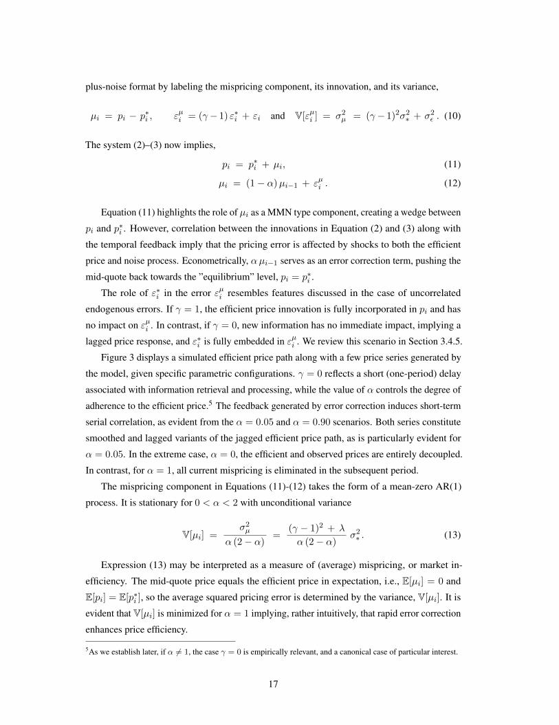
Figure 3: Simulated trajectories for p∗i and pi from model (2) - (3) given two different values of α. The remainingparameters take the values σ2
∗ = 1, γ = 0 and λ = 0.1.
The ”Random-Walk-plus-Noise” Representation
To facilitate comparisons to the extant literature, we couch our model (2)-(3) in a random-walk-
16
plus-noise format by labeling the mispricing component, its innovation, and its variance,
µi = pi − p∗i , εµi = (γ− 1) ε∗i + εi and V[εµi ] = σ2µ = (γ− 1)2σ2
∗ + σ2ε . (10)
The system (2)–(3) now implies,
pi = p∗i + µi, (11)
µi = (1− α)µi−1 + εµi . (12)
Equation (11) highlights the role of µi as a MMN type component, creating a wedge between
pi and p∗i . However, correlation between the innovations in Equation (2) and (3) along with
the temporal feedback imply that the pricing error is affected by shocks to both the efficient
price and noise process. Econometrically, αµi−1 serves as an error correction term, pushing the
mid-quote back towards the ”equilibrium” level, pi = p∗i .
The role of ε∗i in the error εµi resembles features discussed in the case of uncorrelated
endogenous errors. If γ = 1, the efficient price innovation is fully incorporated in pi and has
no impact on εµi . In contrast, if γ = 0, new information has no immediate impact, implying a
lagged price response, and ε∗i is fully embedded in εµi . We review this scenario in Section 3.4.5.
Figure 3 displays a simulated efficient price path along with a few price series generated by
the model, given specific parametric configurations. γ = 0 reflects a short (one-period) delay
associated with information retrieval and processing, while the value of α controls the degree of
adherence to the efficient price.5 The feedback generated by error correction induces short-term
serial correlation, as evident from the α = 0.05 and α = 0.90 scenarios. Both series constitute
smoothed and lagged variants of the jagged efficient price path, as is particularly evident for
α = 0.05. In the extreme case, α = 0, the efficient and observed prices are entirely decoupled.
In contrast, for α = 1, all current mispricing is eliminated in the subsequent period.
The mispricing component in Equations (11)-(12) takes the form of a mean-zero AR(1)
process. It is stationary for 0 < α < 2 with unconditional variance
V[µi] =σ2µ
α (2− α)=
(γ − 1)2 + λ
α (2− α)σ2∗ . (13)
Expression (13) may be interpreted as a measure of (average) mispricing, or market in-
efficiency. The mid-quote price equals the efficient price in expectation, i.e., E[µi] = 0 and
E[pi] = E[p∗i ], so the average squared pricing error is determined by the variance, V[µi]. It is
evident that V[µi] is minimized for α = 1 implying, rather intuitively, that rapid error correction
enhances price efficiency.
5As we establish later, if α 6= 1, the case γ = 0 is empirically relevant, and a canonical case of particular interest.
17

The second factor controlling the degree of inefficiency is the pricing error innovation in
the numerator of Equation (13). This term is small if, all else equal, there is no (local) over- or
under-reaction to latent news (γ = 1), and the idiosyncratic error is minimal (low λ).
In summary, the price dynamics reflects the covariance structure of the innovations to the
mispricing component and the fundamental price, and how these shocks are propagated through
the temporal adjustment process. The covariance structure takes the form,
Σ =
[E[(εµi )2] E[εµi ε
∗i ]
E[εµi ε∗i ] E[(ε∗i )
2]
]=
[(γ − 1)2 + λ γ − 1
γ − 1 1
]σ2∗ . (14)
Equation (14) shows that the off-diagonal entries are non-zero, if and only if γ 6= 1. This point
is discussed further below in our review of the extant literature.
We reiterate that our model, deliberately, is of reduced form and focuses on specific channels
behind salient features of the return dynamics. It is intended as an approximation for short
intraday periods, like 10-30 minutes, for which the factors governing the return dynamics
remain stable. Over longer horizons, the size of the volatility innovation is clearly not constant.
Allowing model parameters to shift across adjacent short intervals, indicating a transition from
one informational regime to another, is in line with the findings of significant time-varying
return autocorrelations in Section 2. We may move from a period of under-reaction to one
of over-reaction due to the shifting nature of the information flow and the broader market
environment.6
3.2 Second Order Return Moments
This section provides model-implied conditions for excess volatility and return serial correlation.
These features are closely related and reflect the impact of MMN versus smoothing in the return
variation process. The latter also affects our ability to identify the drivers behind the price
dynamics from the observed return moments in the absence of auxiliary assumptions.
3.2.1 Excess Return Variation
We recall that the log-return in Equation (3) may be stated as ri = −αµi−1 + (ε∗i + εµi ) . The
following lemma provides an explicit expression for the return variation in this general case.
6The spirit of this approach mimics the assumptions often invoked for developing inference techniques with high-frequency data, see, e.g., Mykland and Zhang (2009) and Bibinger et al. (2014), who explicitly rely on localwindows in which the quantity of interest, in their case return volatility, may be assumed to remain fixed.
18

Lemma 1 (Return Variance). Assume σ2ε > 0, 0 < α ≤ 1, 0 ≤ γ < 2. Then,
V[ri] = α2 V[µi] + (γ2 + λ)σ2∗ (15)
= σ2∗ +
2
2 − αFα(γ, λ) σ2
∗ , (16)
where, for later convenience, for given α, we define Fα(γ, λ) as a function of γ and λ,
Fα(γ, λ) = γ2 + ( 1 − γ ) α + λ − 1.
Proof. Follows by a sequence of straightforward calculations from equation (13).
Equation (15) implies that the return volatility is increasing in σ2∗ and λ. Likewise, due
to the “smoothing” of the price path for low α, the volatility increases with α (for γ < 1).
Finally, as before, the return variation is minimized for γ = α/2, increasing for γ > α/2, and
decreasing for γ < α/2, generalizing the result for the uncorrelated endogenous noise setting
(α = 1).
The following corollary summarizes the conditions for excess volatility in our general
setting, featuring both error correction and endogeneity.
Corollary 1. Assume σ2ε > 0, and 0 < α ≤ 1.
V[ri] ≤ V[r∗i ] if Fα(γ, λ) ≤ 0 , (17)
V[ri] > V[r∗i ] otherwise. (18)
Consequently, the return volatility is lower than the fundamental volatility if price updating
is slow, the extent of noise is low (i.e., α and λ are small), and γ is close to α/2, implying a
variance-minimizing degree of smoothing. The condition Fα(γ, λ) < 0, alternatively, can be
stated as γ2 + λ < 1− α(1− γ). Hence, the two regimes are governed by the relative size of
the effective return smoothing, 1− α(1− γ), and the size of the return innovations, γ2 + λ.
Thus, we have two distinct regimes. In the classical model, γ = 1, the presence of noise,
λ > 0, trivially leads to excess volatility. In contrast, in the presence of partial price adjustments,
the volatility may drop below the level associated with the fundamental innovation process and
generate inverted volatility signature plots.
3.3 Return Auto-Covariances
The determinants of whether returns display excess volatility are also critical for the sign of the
return auto-covariances. This is a consequence of the following lemma and corollary.
19

Lemma 2 (Return Auto-Covariances). Assume σ2ε > 0, 0 < α ≤ 1, , h ≥ 1. Then,
Cov[ri, ri−h] = ψ(h− 1) σ2∗[1 − α (1− γ) − (γ2 + λ)
](19)
= − Fα(γ, λ) ψ(h− 1) σ2∗ , (20)
with ψ(h− 1) = α2−α (1− α)h−1 and ψ(0) = 1, if α = 1.
Proof. See the Supplementary Appendix.
Hence, the relation between 1 − α (1 − γ) and γ2 + λ also governs the sign of the auto-
covariance for the observed returns. We summarize this result in the form of a corollary.
Corollary 2. Assume σ2ε > 0, 0 < α ≤ 1, and h ≥ 1.
Cov[ri, ri−h] ≥ 0 if Fα(γ, λ) ≤ 0 , (21)
Cov[ri, ri−h] ≤ 0 otherwise. (22)
We note that, for 0 < α < 1, the sign of the auto-correlation is identical for all h ≥ 1, so both
”contrarian” and ”momentum” regimes display persistent return dependence. In Section 5, we
seek to identify this feature empirically over short trading intervals.7
For models without endogeneity, γ = 1, return momentum is ruled out, as the necessary
condition, λ < 0, is infeasible – a point further discussed in Section 3.4.1. In contrast, for
γ < 1, momentum regimes are attainable and, contrary to the pure price endogeneity setting of
Section 3.1, this is now possible, e.g., for γ = 0 (as long as λ < 1− α).
It is useful to relate these model implications to our prior empirical evidence. Section 2.1
finds that the returns, on average, display only limited serial dependence. For low values of γ,
this is possible only if 1−α ≈ λ. This is plausible, if the MMN component is small, while prices
impound information swiftly, i.e., 1−α is small as well. More generally, zero return correlation
is consistent with MMN, as long as the impact is mitigated by a certain sluggishness in market
prices. Nonetheless, a large noise component, λ ≥ 1, always induces negative serial correlation
and excess return volatility due to the reversal needed to correct idiosyncratic mispricing.
A natural application of these results is to realized volatility estimation. Traditional realized
variance measures, obtained from cumulative high-frequency squared returns, will be biased
and inconsistent unless the market environment generates a return dynamic that satisfies the
condition for zero excess volatility or, equivalently, for no (significant) return serial correlation,
namely, γ2 + λ ≈ 1 − α (1− γ) or Fα(γ, λ) ≈ 0.
7In contrast, α > 1 implies that the signs alternate for h > 1. Such cycles may be plausible over longer horizons,but abrupt alterations in the return dependencies across short intraday intervals are counterfactual.
20
Finally, note that for given α and λ, scenarios for which |γ − α/2| are identical, e.g., the
cases γ = 0 and γ = α, yield the same return variances and autocovariances. We will discuss
these aspects in more detail in the context of statistical identification in Section 4.1.
3.4 Nested Models
Our model captures basic structural mechanisms from alternative market microstructure ap-
proaches within a uniform setting, providing a starting point for identifying strengths and
limitations of existing paradigms. Because we nest several important special cases, our em-
pirical work should help shed light on which models best approximate salient features of the
high-frequency return process. A second objective is to highlight the identification issues that
arise in microstructure models with a latent endogenous noise component. This often-overlooked
feature becomes evident, as we summarize the empirical implications of various models below.
3.4.1 The Classical Model with Idiosyncratic Noise Autocorrelation
A critical feature of our model (2)–(3) is the allowance for noise endogeneity by having γ 6= 1.
In fact, if γ = 1 then, independently of the noise dynamics, we obtain,
Σ =
[E[(εµi )2] E[εµi ε
∗i ]
E[εµi ε∗i ] E[(ε∗i )
2]
]=
[λ 0
0 1
]σ2∗ .
The absence of correlation among the innovations has important ramifications. Letting ∆µi =
µi − µi−1, for any stationary noise dynamics and integers i, j, we have E[ ε∗i ∆µj ] = 0 and,
ri = pi − pi−1 = ε∗i + ∆µi . (23)
It follows that the actual return variation always exceeds the efficient return variation,
E[ r 2i ] = σ2
∗ + E[ (∆µi)2 ] ≥ σ 2
∗ ,
and the return variance and autocovariances take the form in equations (8) –(9). It implies that,
uniformly, the volatility signature plots should lie above the efficient variance. This is at odds
with the evidence in Section 2, as the signature plots often drop sharply at higher frequencies.
We reiterate that this feature arises, even with dependence in the return series induced by
serial correlation in the noise process. Our model specification (11) and (12) now implies
pi = p∗i + µi , (24)
µi = (1− α)µi−1 + εi , (25)
21
with E[εi ε∗i ] = 0 and E[ εi µj ] = 0 for all integers i, j. Hence, in our parametric setting, the
mispricing component, µi , follows an AR(1) process, inducing return dependence for α 6= 1.
This has empirical relevance for measures using high-frequency features, such as the bid-ask
spread, the price grid and order splitting induce serial dependence in both transaction and
quote returns. Recognizing this issue, the original realized volatility estimation procedures
employ sparse sampling, e.g., Andersen and Bollerslev (1998). Subsequently, a variety of robust
statistical approaches were proposed, including realized kernels, pre-averaging, multi-scale,
or spectral procedures, e.g., Barndorff-Nielsen et al. (2008b), Jacod et al. (2009), Zhang et al.
(2005), and Bibinger et al. (2014). A recent development of simple procedures attaining the
same objective is given by Da and Xiu (2019).
3.4.2 The Classical Model
The i.i.d. noise model is obtained from the model in the preceding section by, in addition,
imposing α = 1, so we have E[εi ε∗i ] = 0 and,
pi = p∗i + εi . (26)
Thus, fundamental news is embodied instantaneously and past pricing errors are corrected
without delay, so shocks fully dissipate by the next observation, yielding V[ri] = σ2∗(1 + 2λ)
and Cov[ri , ri−1] = −λσ2∗ . That is, instant error correction implies negative first-order serial
correlation, but also no return correlation beyond lag one.
This scenario corresponds to the “classic” random-walk-plus-iid-noise model, see, e.g.,
Zhou (1996), Ait-Sahalia et al. (2005) and Bandi and Russell (2008). It still provides the
basic reference for empirical microstructure effects, yet it rules out both feedback effects and
noise endogeneity. The model is rejected, if we find significant evidence of 0 < α < 1, and,
secondarily, γ 6= 1. In fact, these conditions apply for a large set of subintervals in Section 5.2,
pointing towards serious empirical shortcomings of the classic model.
3.4.3 The Uncorrelated Endogenous Noise Model
As discussed in Section 3.4.2, imposing α = 1 generates a scenario with endogenous, but
serially uncorrelated noise, where pi = p∗i + (γ− 1) ε∗i + εi , and the first-order autocovariance
equals Cov(ri , ri−1) = [(1 − γ) γ − λ] σ 2∗ . The specification is consistent with positive
return dependence if γ < 1 , i.e., the concurrent return innovation does not fully incorporate the
efficient price innovation. In this setting, the fundamental return variation may be estimated
consistently through a simple first-order lag adjustment to the realized volatility estimator, as
originally suggested by Zhou (1996).
22

The general point is that noise endogeneity and information feedback are distinct features
and have different implications. The endogeneity can alter the sign of the first-order return
autocorrelation, while the noise correlation generates longer lasting correlation effects. One
objective of this paper is to determine conditions under which we can identify the underlying
source of noise from the observed high-frequency return dependencies.
3.4.4 The Amihud-Mendelson Model
Our model (2)–(3) modifies the standard representation to allow for economic mechanisms
that generate longer-run return dependence. Meanwhile, the finance literature contains several
models designed to accommodate low-frequency serial correlation. Prominent models include
Amihud and Mendelson (1987) and Hasbrouck and Ho (1987). Specifically, the model by
Amihud and Mendelson (1987) emerges as a special case by setting γ = α, implying,
pi = (1 − α) pi−1 + αp∗i + εi . (27)
In this scenario, the mid-quote price is a weighted average of the past price and the current
efficient price, with an innovation term, that is uncorrelated with the efficient price innovation.
The price dynamics in Equation (27) mimics the one in Equation (3), with the notable
difference that the price adjustment in the latter is based on the discrepancy between the lagged
observed and past efficient price. Importantly, the model allows for both noise endogeneity
and feedback effects through an error correction mechanism, while providing a parsimonious
and readily identifiable model. The main drawback is the tight link between the strength of
endogeneity and speed of error correction via the condition γ = α.
Note that Amihud and Mendelson (1987) seek to capture daily return dynamics. In that
context, updating based on the current efficient price (established over a full trading day) is
sensible relative to one-day-old information. In a high-frequency setting, featuring incessant
order book revisions, multiple trades per second, and nearly continuous news feeds, it is less
plausible that traders have the capability, and all relevant information, to gauge the efficient
price every instant. Instead, updates may occur with a delay of a few seconds. As such, Equation
(3) seems more suitable at high frequencies.
3.4.5 The Information Delay Model
An alternative specification, yielding the identical first- and second-order return moments as the
Amihud and Mendelson (1987) model, may be obtained via a different economic mechanism.
As noted in Section 3.2, γ = 0 implies that even well-informed agents respond to newly arriving
information with a minor delay. This leads to a lagged price response and feedback – features
23
that appear empirically relevant. Moreover, the delay and feedback effects can be stronger
or weaker depending on the information and market environment at the time, motivating our
approach of keeping model parameters fixed only over short intraday intervals.
In this “information processing delay” representation, the only contemporaneous shock
impacting the price is idiosyncratic noise. Simultaneously, the price adjusts to past pricing
errors, enabling the efficient price innovations to govern the intermediate return dynamics, as
the market disentangles the noise and fundamental shocks to prices.
Letting γ = 0, Equations (2)–(3) generate the following price dynamic,
pi = (1 − α) pi−1 + αp∗i−1 + εi . (28)
A few comments are in order. First, since ε∗i is latent and uncorrelated with εi, we obtain
an equivalent representation by relabeling p∗i−1 as p∗i . But this renders Equations (27) and (28)
identical. In other words, we cannot separately identify the two models – they generate the
identical process for the observed returns. This point was briefly mentioned in Section 3. It
complicates identification and inference in general – an issue we discuss in depth in Section 4.1.
Second, the covariance structure for the innovations now takes the simple form
Σ =
[E[(εµi )2] E[εµi ε
∗i ]
E[εµi ε∗i ] E[(ε∗i )
2]
]= σ2
∗
[1 + λ −1
−1 1
].
This result reflects that efficient innovations are incorporated into prices with a delay, so the
mispricing component must absorb the full impact of any concurrent ε∗i shock, rendering the
noise process endogenous. In this scenario, the return dynamics, reflecting the error correction
mechanism, is the only source of coherence between market and efficient prices. Hence, the
market is in a perpetual state of transition, driven by an ongoing process of price discovery.
Conceptually, this separates our specification from standard microstructure models in which
prices are in equilibrium, except for short-lived distortions induced by exogenous noise shocks.
Third, the “information delay” model differs from the high-frequency Amihud and Mendel-
son (1987) model, as the latter has a covariance structure identical to the general representation
(14), but with γ = α. For either model, once information processing is initiated, it proceeds at
a rate governed by α. The latency of the efficient innovation means that we cannot determine
if this occurs with a temporal delay or not. This notwithstanding, the incomplete and delayed
price adjustment renders the noise endogenous. Typically, such endogeneity is imposed through
explicit statistical assumptions, see, e.g., Kalnina and Linton (2008), but it is endowed with a
more structural interpretation in our specification.
In summary, our information delay model – or high-frequency reinterpretation of Amihud
24

and Mendelson (1987) – featuring just three free parameters, (α, λ, σ∗), endows the asset pricing
process with dynamic properties reflecting distinct underlying economic factors. The empirical
evidence in Section 5 illustrates how this fully identifiable variant of our model captures salient
features of the short-run dynamics, providing a superior framework for assessing the separate
economic forces at play relative to traditional microstructure representations.
3.5 Realized Volatility Measures
This section reviews the implications of the preceding results for realized volatility measures
computed from return data generated by model (2)–(3). The realized volatility for interval [0, T ],
using equidistant log-price observations, pi∆ , i = 0, . . . , n = n(∆) = bT/∆c, is obtained as
RVT (∆) =
n(∆)∑i=1
(pi∆ − p(i−1)∆
) 2=
n(∆)∑i=1
( ri∆ ) 2 , (29)
where we have chosen the notation n(∆) to make the dependence of n on ∆ explicit.
In the frictionless variant of our model with α = γ = 1 and λ = 0, we have
E [RVT (∆) ] = T σ2∗ . (30)
In the case of general exogenous noise, ri = ε∗i + ∆µi , as discussed in Section 3.4.1, we
find, in analogy to the result established there, that,
E [RVT (∆) ] = T[σ2∗ + E[ (∆µi)
2]≥ T σ2
∗ . (31)
This result reiterates a point stressed by Hansen and Lunde (2006) – the realized volatility
measure, absent endogenous noise, cannot be downward biased. Moreover, the extent of any
upward bias is determined by the properties of the noise process. The usual assumption is that
every price observation contains a noise component unrelated to the sampling interval, so ∆µi
constitutes an Op(1) term which, for ∆→ 0, dominates the Op(√
∆) term stemming from the
efficient price innovation. This generates an increasing upward bias with sampling frequency,
and a positively sloped volatility signature plot for ∆→ 0.
As noted previously, the above is, generally, not factual. The illustrations in Figure 1 show
that, as the sampling frequency increases, the volatility signature plot is sharply upward sloping
in some periods and sharply downward sloping in other periods. The discussion in Section
3.4.1 reminds us that the latter is possible only if the noise is endogenous. Specifically, for our
25

parametric model (2)–(3), but imposing exogenous noise, γ = 1, we obtain
E [RVT (∆) ] = T [ 1 + 2λ ] σ2∗ . (32)
In contrast, for the full parametric model with γ 6= 1,
E [RVT (∆) ] = T
[1 +
2
2 − αFα(γ, λ)
]σ2∗ . (33)
As before, the sign of Fα(γ, λ) determines whether the return volatility measure is upward or
downward biased. Both cases are empirically important, as they each occur with regularity,
showing that a (time-varying) degree of exogenous and endogenous noise is required to capture
the observed features of the volatility process for individual large capitalization equity returns.
4 Statistical Inference
4.1 Identification
Section 3 shows that our general model (2)–(3) is not uniquely identified from the second-order
return moments. This type of identification issue is well recognized. There are two distinct
sets of assumptions regarding the noise, leading to starkly different procedures. One approach
casts the model in continuous time and conducts inference via an in-fill asymptotic scheme,
where the number of observations (ticks) diverges within a fixed interval. In this case, the noise
dependence can generally be identified, because the size of the tick-by-tick innovations in the
efficient price shrinks in line with the interval, while the magnitude of the noise shocks are
invariant with respect to sampling frequency, so the noise is asymptotically “big,” allowing for
nonparametric identification. A thorough development of this approach is provided by Jacod
et al. (2017); see also the discussion in Li and Linton (2016). Likewise, Da and Xiu (2019)
obtain consistent inference from a tick-time MA(q) noise process in a continuous-time setting
with independence between noise and efficient price, but otherwise very general assumptions.
In contrast, if the noise dependence is fixed in calendar time, asymptotic inference requires an
increasing time horizon. In this case, identification hinges on the stipulation that the fundamental
price process is a (semi-)martingale, while the noise is stationary. The latter implies an element
of mean reversion but, without auxiliary assumptions, this can only be ascertained with precision
over longer time intervals. Moreover, dependence between the noise and fundamental price
process complicates identification even further, as noted in Ait-Sahalia et al. (2006). Typically,
one can only accomplish this task via careful parametric modeling.
Our general discrete-time model illustrates the latter point. Without endogeneity (γ = 1),
26

the system is identified through the parametric specification, but once such dependence is
introduced, we have only partial identification. We can estimate the key parameter determining
the fundamental price volatility, namely σ2∗ , but the finer details of the noise dynamics are elusive,
as the second-order moments of observed returns cannot disentangle the delay with which the
observed price incorporates the fundamental innovation from the relative size (variance) of the
noise component. Specifically, the issue revolves around separate identification of λ and γ.
Both impact the return variation and autocovariances, (15) and (20), only through the function
Fα(γ, λ) = γ2 − αγ + α+ λ− 1. Thus, any combinations of γ and λ yielding the same value
for Fα(γ, λ) imply identical second-order moments. In contrast, it is readily shown that α and
σ2∗ are identifiable. Henceforth, in this section, we often abbreviate Fα(γ, λ) by Fα.
We may exploit additional information by imposing natural constraints on γ and λ, such
as non-negativity. Yet, whenever they are not on the boundary, any small shift in γ may be
offset by a compensatory shift in λ, leaving Fα unaltered. Since Fα is linear in λ and quadratic
in γ, fixing γ identifies λ but, as illustrated in Section 3, fixing λ does not generally uniquely
identify γ, as the implied second-order polynomial in γ has two roots. Accordingly, scenarios
with identical values for |γ − α/2| are observationally equivalent. When estimating the general
model, we therefore focus on the lower-dimensional vector (α, σ2∗ , Fα), with values for Fα
consistent with a range of (γ, λ) combinations for given return dynamics.
To illustrate the geometry of non-identification regions for (γ, λ), we consider two scenarios
associated with positive and negative return autocorrelations, respectively. In Regime I, we
choose the parameter values α = 0.835, σ2∗ = 0.986 · 10−8 and Fα = −0.100 producing a
positive first-order autocorrelation of 0.087. In Regime II, we set α = 0.976, σ2∗ = 0.524 · 10−8
and Fα = 0.091, resulting in a negative first-order autocorrelation of −0.074. These values for
α, σ2∗ and Fα correspond to the median estimates α, σ2
∗ and Fα obtained across local 10-minute
intervals with positive and negative return autocorrelations, respectively, in Section 5.
27

0.0 0.2 0.4 0.6 0.8 1.0 1.2γ
0.0
0.1
0.2
0.3
0.4λ
F<0
F>0
Regime Iλ= λ(γ)Fα(γ, λ) = 0
0.0 0.2 0.4 0.6 0.8 1.0 1.2γ
0.0
0.1
0.2
0.3
0.4
λ
γ<1 γ>1
F<0
F>0
Regime II
Figure 4: The dashed blue lines describe admissible values of (γ, λ), corresponding to Regime I (left plot) andRegime II (right plot). Regime I has α = 0.835, σ2
∗ = 0.986 · 10−8 and Fα = −0.100 and generates positivereturn autocorrelation. Regime II has α = 0.976, σ2
∗ = 0.524 · 10−8 and Fα = 0.091 and generates negativeautocorrelation. The solid black lines represent values of (γ, λ) which solve equation Fα(γ, λ) = 0 for a given α.
Figure 4 depicts the admissible loci of (γ, λ) for Regimes I (left) and II (right), imposing
non-negativity. The shaded rectangular area indicates the range of values γ and λ can take given
the remaining parameters. The admissible (γ, λ) combinations are indicated by the dashed blue
line, with λ treated as a function of γ and the values of Fα and α for the corresponding regime.
The solid black line depicts the loci of (γ, λ) solving Fα(γ, λ) = 0 for a given α. All
points below this line imply Fα(γ, λ) < 0, whereas all points above indicate Fα(γ, λ) > 0.
Accordingly, for Regime I (positive autocorrelation) and negative Fα, all admissible pairs (γ, λ)
are located below the parabolic curve Fα(γ, λ) = 0. In contrast, for Regime II (negative
autocorrelation), all admissible (γ, λ) combinations lie above Fα(γ, λ) = 0.
This analysis delivers maximum admissible values for γ and λ in a given regime. For λ, it
is attained at the level of γ that minimizes the return variance, i.e., γ = α/2,
λmax =α2
4− α + Fα + 1. (34)
Correspondingly, it is readily seen that γmax is attained for λ = 0, so that,
γmax =α
2+√λmax. (35)
This provides algebraic upper bounds given estimates for the identified parameters (α, σ2∗ , Fα).
We further note that the maximum γ satisfying the boundary condition Fα(γ, λ) = 0 is
attained for λ = 0 and equals unity. Therefore, Fα < 0 implies γmax < 1, and Fα > 0 implies
γmax > 1. This feature is nicely illustrated in Figure 4. If Fα < 0 (Regime I), the dashed
curve λ(γ) is below the black curve (Fα(γ, λ) = 0), crossing the horizontal axis below 1, and
28

γmax < 1. If Fα > 0 (Regime II), the situation is reversed. Here, overreactions to return
innovations (γ > 1) only occur for Fα > 0, implying negative first-order autocorrelation.
These identification relations have direct implications for the special cases of our model, dis-
cussed in Section 3.4. Firstly, the equivalence between the Amihud-Mendelson and Information
Delay model follows from the fact that γ = α and γ = 0 both imply Fα(γ, λ) = α + λ − 1.
Secondly, the classic i.i.d. noise model implies γ = 1 and Fα(1, λ) = λ > 0, excluding positive
serial correlation. As demonstrated in Section 2, this is counterfactual, and the associated
estimates of the efficient return variance, σ2∗ , will generally be biased.
The endogenous, uncorrelated noise model of Section 3.4.3 with α = 1 implies F1(γ, λ) =
γ2 − γ + λ. In contrast to the classical model with idiosyncratic noise, this allows for a
positive first-order return autocorrelation. Due to the constraints discussed above, we have
F1(γ, λ) ≥ −14 , thus the first-order autocorrelation must fall within (−1
2 ,12).
Finally, by fixing γ, the information delay (equivalently, Amihud-Mendelson) model allows
for identification of all remaining parameters without imposing additional constraints on the
return dynamics. This specification allows for only partial instant incorporation of fundamental
information along with the feedback mechanism associated with dynamic price discovery.
4.2 Estimation
For estimation purposes, it is convenient to restate the model as
ri = −αµi−1 + εi,
µi = (1− α)µi−1 + εµi ,
where εi = γε∗i + εi and εµi = εi − ε∗i = (γ − 1)ε∗i + εi. Then, returns ri are driven by a latent
variable µi following an AR(1) process with covariance structure given by
E[ εiµi+h ] = (1− α)h(γ2 + λ− γ
)σ2∗ , ∀h ≥ 0,
E[ εiµi−h ] = 0, ∀h > 0,
E[ εiεµi ] = [ γ(γ − 1) + λ ] σ2
∗,
E[ εiεµi−h ] = 0, ∀h 6= 0.
As illustrated in the Supplementary Appendix, the model can be straightforwardly estimated
by maximum likelihood using the prediction error decomposition, see, e.g., Harvey (1989),
29
yielding the log-likelihood
`(Y, θ) = −1
2
T∑i=1
ln(si) −1
2
T∑i=1
ν2i
s2i
, (36)
where νi denote (optimal) linear predictions of ri given the past returns (ri−1, . . . , r1), and
s2i = E[ν2
i |ri−1, . . . , r1] denotes the conditional variance. Assuming Gaussianity for εi and ε∗i ,
`(Y, θ) can be readily computed by the Kalman filter based on a reformulation of the model
in terms of a linear state-space system. If the errors ε∗i and εi are not normally distributed,
Equation (36) instead has the interpretation of a quasi likelihood function yielding consistency
of parameter estimates provided that the second order moments of returns are correctly specified.
In this case, the linear predictions of the state variables are not optimal among all prediction
functions, but remain the best linear ones, see the Supplementary Appendix, Section 2 for
details.
We reiterate that our estimation approach differs fundamentally from the usual infill asymp-
totic procedures applied for realized volatility estimation. This reflects our finding of prolonged
periods of persistent return serial correlation and the corresponding model feature involving a
temporal feedback mechanism. To capture such temporal effects, the analysis is most naturally
cast in discrete time, using a fixed ∆ > 0. In this context, ML inference provides a standard√T convergence rate for fixed ∆ and T →∞.
5 Evidence from Model Estimation
In this section, we explore the high-frequency price dynamics within local intraday intervals by
estimating variants of the model introduced in Section 3, using the sample of mid-quote returns
for the 100 stocks described in Section 2.
5.1 Parameter Estimates
We estimate the model by maximum likelihood using the Kalman filter, as described in Section
4.2 and the Supplementary Appendix. We obtain estimates for each stock in the NASDAQ 100
over the first 61 trading days of 2014, for each T = 10 min interval, sampling at the ∆= 2 second
frequency. As such, our empirical analysis utilizes a total of 237,900 local intervals.
Since the parameters of the general model are only partially identified, we momentarily
impose the convenient restriction, γ = 0. In Section 4.1, we demonstrated that γ = 0 is
admissible irrespective of the regime governing the return dynamics. Hence, the parameters
α, σ2∗ and Fα(γ, λ) remain unrestricted and are uniquely identified, with λ simply adjusting to
30

accommodate the estimated value for Fα(0, λ) = F . Next, we remove the γ = 0 constraint
and instead determine the set of (γ, λ) values compatible with Fα(γ, λ) = F . This allows us to
readily obtain the upper bounds for λmax and γmax given by Equations (34)-(35).
5.1.1 Empirical Distribution of Parameter Estimates
Figure 5 displays the empirical distributions of the parameter estimates obtained across all
stocks in the first, fourth and fifth quintile, respectively, sorted according to the intensity of
quote-midpoint revisions, as detailed in Section 2. All distributions appear unimodal and
approximately symmetric, apart from the distinct right skew in the σ2∗ distribution.
In Group 1, the α estimates have a mode around 0.90, corroborating the hypothesis of a
feedback effect and mildly sluggish price adjustments. The distribution of γmax is centered
around 1, .consistent with our prior finding in Table 1 of an empirical first-order return autocor-
relation around zero, but with a significant number of both positive and negative coefficients.
The two regimes imply, respectively, that γmax < 1 and γmax > 1, with these values attained
only for λ = 0, as illustrated also by the left and right panels of Figure 4. Because the returns,
invariably, embody some degree of noise – price discreteness and other frictions are non-trivial
at high frequencies – we expect λ > 0. Hence, the relevant parameter vector must imply
γ < γmax, reflecting a leftward movement along the dashed curves in Figure 4, starting from
(γ, λ) = (γmax, 0). We conclude that, for a majority of the local intervals, γ < 1.
The above discussion reflects the fundamental identification issues that typically arise in
microstructure models with latent and endogenous noise. Our model has two separate sources
of non-martingale return behavior. Idiosyncratic noise is “corrected” over time, inducing
negative return serial dependence, while incomplete incorporation of fundamental innovations –
endogeneity – induces positive dependence, as market prices subsequently adjust to the shift in
the efficient price (for α/2 < γ < 1). Therefore, given a parameter vector being compatible
with a given level of serial correlation, it is possible to increase both the strength of idiosyncratic
noise and the endogeneity (initial under-reaction to fundamental news) and have the effects
cancel, leaving the return autocorrelation pattern unchanged.
Our results imply that, for most intervals, the return dynamics is affected by endogenous
noise. This typically induces a smoother price path, and the overall effect is a positive or negative
return autocorrelation depending on the relative size of the idiosyncratic noise component, λ.
Note also that some of the local intervals featuring negative return autocorrelation may imply
γ > 1, indicating an information environment where agents are (overly) concerned about
asymmetric information and tend to overreact to information signals, generating “overshooting.”
For such episodes, there is an additional trigger for price reversals that reinforces the impact of
idiosyncratic noise.
31

0.6 0.8 1.0 1.2α
0
2
4
6
8
10
Group 1 Group 4 Group 5
0.0 0.2 0.4 0.6 0.8σ2*
1e−7
0.0
0.2
0.4
0.6
0.8
1.0 1e8
0.0 0.2 0.4 0.6λmax
0
5
10
15
−0.4 −0.2 0.0 0.2 0.4corr(rt+1, rt)
0
2
4
6
8
10
0.6 0.8 1.0 1.2 1.4γmax
0
2
4
6
8
−0.4 −0.2 0.0 0.2 0.4Fα(γ, λ)
0
5
10
15
Figure 5: The figure depicts empirical distributions of the parameter estimates (under the restriction γ = 0)obtained from T = 10 min intervals sampled at frequency ∆= 2 sec. Results are reported for the stocks in the 1st,4th and 5th group sorted by the average number of daily mid-quote revisions (20 stocks per group) for the first 61trading days in 2014. In total, each density is constructed from parameter estimates across 47,580 local intervals.
Furthermore, our upper bound estimates for the noise-to-signal ratio, λmax, fall below
0.4 for most intervals. This confirms findings in the recent literature of a small idiosyncratic
noise component for large capitalization stocks. Consistent with the evidence in Section 2, the
distribution of the autocorrelation estimates for Group 1 has a small positive mode and a right
skew, indicating that, for liquid stocks, regimes with positive return autocorrelation are common
and, perhaps, even in the majority.
32

For the less liquid stocks in Group 4, we find a slightly lower degree of return dependence,
a lower level of fundamental volatility, and more rapid error correction. To interpret these
findings, it is useful to have actual estimates for the relative degree of idiosyncratic noise, but
this is complicated due to the lack of separate identification for λ. We return to this issue below.
In Group 5, the estimates of α and λmax are somewhat higher on average, have smaller
dispersion around the mode and are distinctly right-skewed. That is, less liquid stocks with
fewer quote revisions and larger relative tick size generate returns that are noisier and react
more strongly to past pricing errors. Consequently, the model-implied return autocorrelations
are predominantly negative, as also indicated by the slight left skew in the associated empirical
distribution. Table 4 of the Supplementary Appendix provides detailed summary statistics for
the parameter estimates in each of the five liquidity quintiles. The identical qualitative patterns
are present in all quintiles and the relevant statistics shift monotonically across the quintiles,
corroborating our earlier findings. We stress, however, that Group 5 constitutes an outlier and
may be unduly impacted by pronounced illiquidity. The results for the initial 10 minutes of
trading, reported in Figure 1 of the Supplementary Appendix, corroborates this conjecture.
The trading in the opening period is very active as overnight news and accumulated orders are
processed by the market. Consequently, Group 5 stocks are also quite liquid over this interval,
and Figure 1 of the Supplementary Appendix confirms that the distribution of the parameter
estimates are closely aligned with those in the other groups. In short, the general estimates for
Group 5 are likely heavily impacted by microstructure frictions, and we focus our attention on
the other groups in the sequel.
The fully identified Information Delay model from Section 3.4.5 or, equivalently, the
Amihud-Mendelson model in Section 3.4.4 enables us – at the cost of imposing one additional
restriction – to shed light on the trade-off between γ and λ. This model retains both the
noise endogeneity and error correction mechanism, but α now governs the strength of each.
Importantly, the model is fully consistent with our general model estimates, as the permissible
combinations of (γ, λ) always allow for γ = 0 or, equivalently, γ = α. In this scenario, the
fundamental price innovation is incorporated only partially, and possibly with a delay, into the
current market price. The distribution of the estimates for the relative size of the idiosyncratic
noise component, λ, in this model is displayed in Figure 6.
We observe an upward shift in λ for Group 4 versus Group 1. Group 2 and 3 stocks (not
depicted) have λ distributions located between those of Group 1 and 4, with Group 2 closer
to Group 1, indicating a monotonic pattern. This suggests, quite intuitively, that more active
stocks display less idiosyncratic noise. For a higher λ, traders interpret any given price change
as relatively more likely to reflect noise than information, increasing the α coefficient and thus
the willingness to trade against recent price moves, pulling the return autocorrelation towards
33
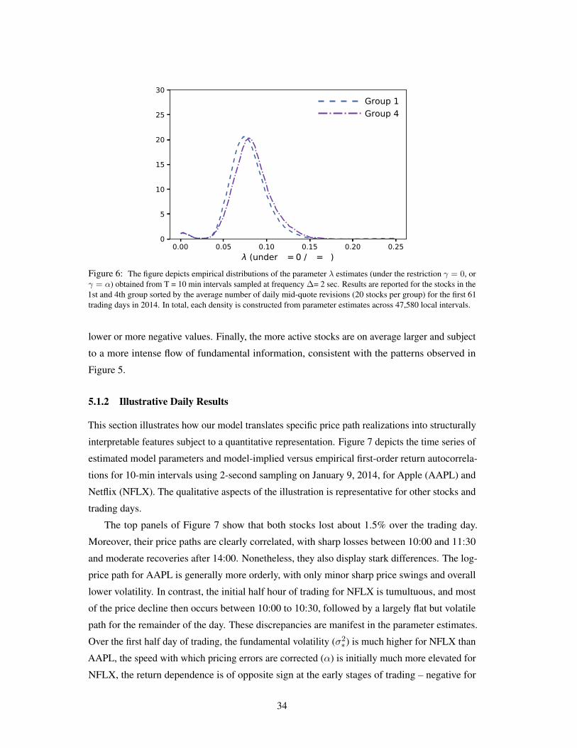
0.00 0.05 0.10 0.15 0.20 0.25λ (under γ=0 / γ=α)
0
5
10
15
20
25
30Group 1Group 4
Figure 6: The figure depicts empirical distributions of the parameter λ estimates (under the restriction γ = 0, orγ = α) obtained from T = 10 min intervals sampled at frequency ∆= 2 sec. Results are reported for the stocks in the1st and 4th group sorted by the average number of daily mid-quote revisions (20 stocks per group) for the first 61trading days in 2014. In total, each density is constructed from parameter estimates across 47,580 local intervals.
lower or more negative values. Finally, the more active stocks are on average larger and subject
to a more intense flow of fundamental information, consistent with the patterns observed in
Figure 5.
5.1.2 Illustrative Daily Results
This section illustrates how our model translates specific price path realizations into structurally
interpretable features subject to a quantitative representation. Figure 7 depicts the time series of
estimated model parameters and model-implied versus empirical first-order return autocorrela-
tions for 10-min intervals using 2-second sampling on January 9, 2014, for Apple (AAPL) and
Netflix (NFLX). The qualitative aspects of the illustration is representative for other stocks and
trading days.
The top panels of Figure 7 show that both stocks lost about 1.5% over the trading day.
Moreover, their price paths are clearly correlated, with sharp losses between 10:00 and 11:30
and moderate recoveries after 14:00. Nonetheless, they also display stark differences. The log-
price path for AAPL is generally more orderly, with only minor sharp price swings and overall
lower volatility. In contrast, the initial half hour of trading for NFLX is tumultuous, and most
of the price decline then occurs between 10:00 to 10:30, followed by a largely flat but volatile
path for the remainder of the day. These discrepancies are manifest in the parameter estimates.
Over the first half day of trading, the fundamental volatility (σ2∗) is much higher for NFLX than
AAPL, the speed with which pricing errors are corrected (α) is initially much more elevated for
NFLX, the return dependence is of opposite sign at the early stages of trading – negative for
34
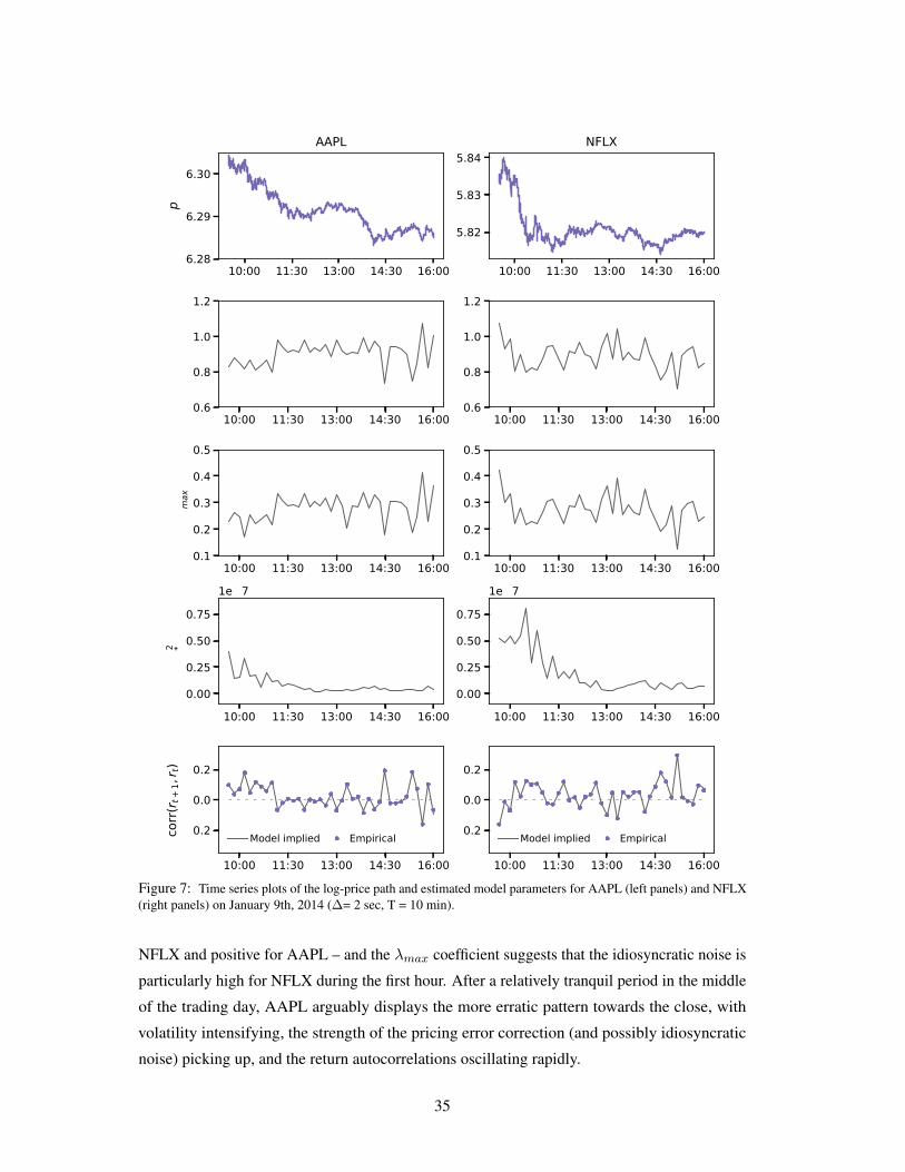
10:00 11:30 13:00 14:30 16:006.28
6.29
6.30p
AAPL
10:00 11:30 13:00 14:30 16:00
5.82
5.83
5.84NFLX
10:00 11:30 13:00 14:30 16:000.6
0.8
1.0
1.2
α
10:00 11:30 13:00 14:30 16:000.6
0.8
1.0
1.2
10:00 11:30 13:00 14:30 16:000.1
0.2
0.3
0.4
0.5
λ max
10:00 11:30 13:00 14:30 16:000.1
0.2
0.3
0.4
0.5
10:00 11:30 13:00 14:30 16:000.00
0.25
0.50
0.75
σ2 *
1e−7
10:00 11:30 13:00 14:30 16:000.00
0.25
0.50
0.751e−7
10:00 11:30 13:00 14:30 16:00
−0.2
0.0
0.2
corr(
r t+1,r t)
Model i plied E pirical
10:00 11:30 13:00 14:30 16:00
−0.2
0.0
0.2
Model i plied E pirical
Figure 7: Time series plots of the log-price path and estimated model parameters for AAPL (left panels) and NFLX(right panels) on January 9th, 2014 (∆= 2 sec, T = 10 min).
NFLX and positive for AAPL – and the λmax coefficient suggests that the idiosyncratic noise is
particularly high for NFLX during the first hour. After a relatively tranquil period in the middle
of the trading day, AAPL arguably displays the more erratic pattern towards the close, with
volatility intensifying, the strength of the pricing error correction (and possibly idiosyncratic
noise) picking up, and the return autocorrelations oscillating rapidly.
35
Hence, despite striking similarities, the market environment for the two stocks evolved
differently. For NFLX, traders may have sensed that (unknown) new information needed to
be incorporated into the price at the open. After an initial phase of rapid moves up and down,
characterized by a strong negative return autocorrelation, the sentiment turned bearish, and
the price dropped quickly, while fundamental volatility increased to an even higher level, and
the return serial dependence turned positive. In contrast, AAPL underwent a relatively calm
price decline at a lower level of fundamental price volatility, with positive return autocorrelation
throughout this period, and a lower speed of pricing error correction. Towards the market close,
however, more information uncertainty is apparent in the trading for AAPL than NFLX.
Our model renders distinct and rapidly shifting features of the market environment, as
those noted above, quantifiable and interpretable. The bottom panels of Figure 7 illustrate
how well our model accommodates the observed variation in first-order return autocorrelations.
Importantly, the real objective is not to fit these return moments, but rather to convert them into
a simple structural framework that helps us disentangle the factors driving the market dynamics.
Specifically, a period with observed negative return correlations may reflect either a high degree
of idiosyncratic noise, a low degree of fundamental information flow, a quicker pricing error
correction, or a combination of such attributes. Each scenario translates into a different measure
for the intensity of the information and frictional forces driving the significant intraday variation
in the return autocorrelation regimes documented in Section 2.
5.2 Model Specification Analysis
We now examine whether the introduction of the key parameters, α and γ, provide a statistically
relevant extension to the models for high-frequency asset prices routinely used in the literature.
In particular, the classical model with i.i.d. noise, in Section 3.4.2, arises from our general
model under the parameter restrictions α = 1 and γ = 1.
We first test the null hypothesisH0 : α = 1 against the two-sided alternative,H ′1 : α < 1 and
H ′′1 : α > 1. We employ a Wald test based on QML (”sandwich”) estimates of the asymptotic
covariance. Table 4 reports the rejection frequencies based on a 5% significance level computed
across the 100 stocks and all local intervals with T = 10 minutes and ∆ = 2 seconds.
Despite low power due to the short intervals and despite possibly conservative QML Wald
test statistics, we reject the null hypothesis for approximately 20% of the local intervals.
Interestingly, whereas the null is rejected roughly similarly for more liquid stocks (Groups 1-4),
the rejection rate for the least liquid stocks (Group 5) is considerably higher reaching almost
35%. Moreover, the rejections are almost exclusively due to point estimates of α < 1. This
suggests that the price dynamics reflects a delayed response to both current and past pricing
36
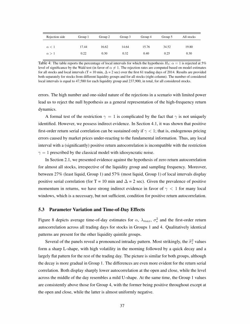
Rejection side Group 1 Group 2 Group 3 Group 4 Group 5 All stocks
α < 1 17.44 16.62 14.64 15.76 34.52 19.80
α > 1 0.22 0.30 0.32 0.40 0.25 0.30
Table 4: The table reports the percentage of local intervals for which the hypothesis H0: α = 1 is rejected at 5%level of significance by the Wald test (in favor of α 6= 1. The rejection rates are computed based on model estimatesfor all stocks and local intervals (T = 10 min, ∆ = 2 sec) over the first 61 trading days of 2014. Results are providedboth separately for stocks from different liquidity groups and for all stocks (right column). The number of consideredlocal intervals is equal to 47,580 for each liquidity group and 237,900, in total, for all considered stocks.
errors. The high number and one-sided nature of the rejections in a scenario with limited power
lead us to reject the null hypothesis as a general representation of the high-frequency return
dynamics.
A formal test of the restriction γ = 1 is complicated by the fact that γ is not uniquely
identified. However, we possess indirect evidence. In Section 4.1, it was shown that positive
first-order return serial correlation can be sustained only if γ < 1; that is, endogenous pricing
errors caused by market prices under-reacting to the fundamental information. Thus, any local
interval with a (significantly) positive return autocorrelation is incompatible with the restriction
γ = 1 prescribed by the classical model with idiosyncratic noise.
In Section 2.1, we presented evidence against the hypothesis of zero return autocorrelation
for almost all stocks, irrespective of the liquidity group and sampling frequency. Moreover,
between 27% (least liquid, Group 1) and 57% (most liquid, Group 1) of local intervals display
positive serial correlation (for T = 10 min and ∆ = 2 sec). Given the prevalence of positive
momentum in returns, we have strong indirect evidence in favor of γ < 1 for many local
windows, which is a necessary, but not sufficient, condition for positive return autocorrelation.
5.3 Parameter Variation and Time-of-Day Effects
Figure 8 depicts average time-of-day estimates for α, λmax, σ2∗ and the first-order return
autocorrelation across all trading days for stocks in Groups 1 and 4. Qualitatively identical
patterns are present for the other liquidity quintile groups.
Several of the panels reveal a pronounced intraday pattern. Most strikingly, the σ2∗ values
form a sharp L-shape, with high volatility in the morning followed by a quick decay and a
largely flat pattern for the rest of the trading day. The picture is similar for both groups, although
the decay is more gradual in Group 1. The differences are even more evident for the return serial
correlation. Both display sharply lower autocorrelation at the open and close, while the level
across the middle of the day resembles a mild U-shape. At the same time, the Group 1 values
are consistently above those for Group 4, with the former being positive throughout except at
the open and close, while the latter is almost uniformly negative.
37

10:00 11:30 13:00 14:30 16:00
0.88
0.90
0.92
0.94
αGroup 1 Group 4
10:00 11:30 13:00 14:30 16:000.25
0.30
0.35
0.40λmax
10:00 11:30 13:00 14:30 16:000.0
0.5
1.0
1.5
2.0 1e−7 σ2*
10:00 11:30 13:00 14:30 16:00−0.04
−0.02
0.00
0.02
0.04corr(rt+1, rt)
10:00 11:30 13:00 14:30 16:00
0.96
0.98
1.00
1.02
1.04
1.06γmax
10:00 11:30 13:00 14:30 16:00−0.08
−0.04
0.00
0.04
0.08Fα(γ, λ)
Figure 8: Intraday plots of average model parameters estimated over the period January - March, 2014 (61 tradingdays in total). Results are reported for the Nasdaq stocks from 1st and 4th groups sorted by the average number ofdaily mid-quote revisions (with 20 stocks in each group) for ∆= 2 sec on intraday intervals T = 10 min.
These features also impact the remaining parameters. For α, we observe an elevation
at the open and close, while there is a mild reverse U-shape across the main phase of the
trading session. The bottom two panels display the maximum γ and λ values consistent with
the fully identified parameters. They merely provide upper bounds and cannot be attained
simultaneously. Specifically, γmax applies for λ = 0, while λmax is achieved for γ = α/2.
Since we, unquestionable, must have λ > 0 to capture idiosyncratic noise stemming from
market frictions, the average γ must be below unity almost uniformly for Group 1 and, likewise,
most of the time in Group 4. Hence, endogenous noise is ubiquitous. These considerations
38
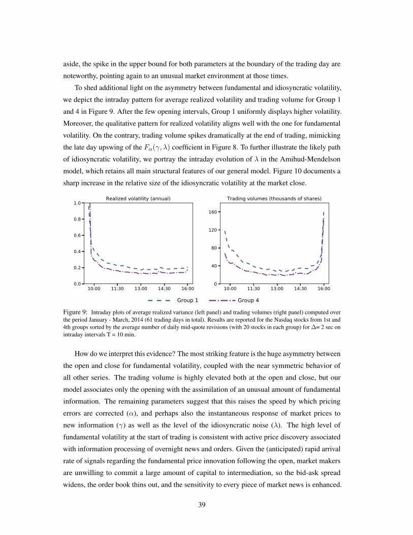
aside, the spike in the upper bound for both parameters at the boundary of the trading day are
noteworthy, pointing again to an unusual market environment at those times.
To shed additional light on the asymmetry between fundamental and idiosyncratic volatility,
we depict the intraday pattern for average realized volatility and trading volume for Group 1
and 4 in Figure 9. After the few opening intervals, Group 1 uniformly displays higher volatility.
Moreover, the qualitative pattern for realized volatility aligns well with the one for fundamental
volatility. On the contrary, trading volume spikes dramatically at the end of trading, mimicking
the late day upswing of the Fα(γ, λ) coefficient in Figure 8. To further illustrate the likely path
of idiosyncratic volatility, we portray the intraday evolution of λ in the Amihud-Mendelson
model, which retains all main structural features of our general model. Figure 10 documents a
sharp increase in the relative size of the idiosyncratic volatility at the market close.
10:00 11:30 13:00 14:30 16:000.0
0.2
0.4
0.6
0.8
1.0Realized volatility (annual)
Group 1 Group 4
10:00 11:30 13:00 14:30 16:000
40
80
120
160
Trading volumes (thousands of shares)
Figure 9: Intraday plots of average realized variance (left panel) and trading volumes (right panel) computed overthe period January - March, 2014 (61 trading days in total). Results are reported for the Nasdaq stocks from 1st and4th groups sorted by the average number of daily mid-quote revisions (with 20 stocks in each group) for ∆= 2 sec onintraday intervals T = 10 min.
How do we interpret this evidence? The most striking feature is the huge asymmetry between
the open and close for fundamental volatility, coupled with the near symmetric behavior of
all other series. The trading volume is highly elevated both at the open and close, but our
model associates only the opening with the assimilation of an unusual amount of fundamental
information. The remaining parameters suggest that this raises the speed by which pricing
errors are corrected (α), and perhaps also the instantaneous response of market prices to
new information (γ) as well as the level of the idiosyncratic noise (λ). The high level of
fundamental volatility at the start of trading is consistent with active price discovery associated
with information processing of overnight news and orders. Given the (anticipated) rapid arrival
rate of signals regarding the fundamental price innovation following the open, market makers
are unwilling to commit a large amount of capital to intermediation, so the bid-ask spread
widens, the order book thins out, and the sensitivity to every piece of market news is enhanced.
39
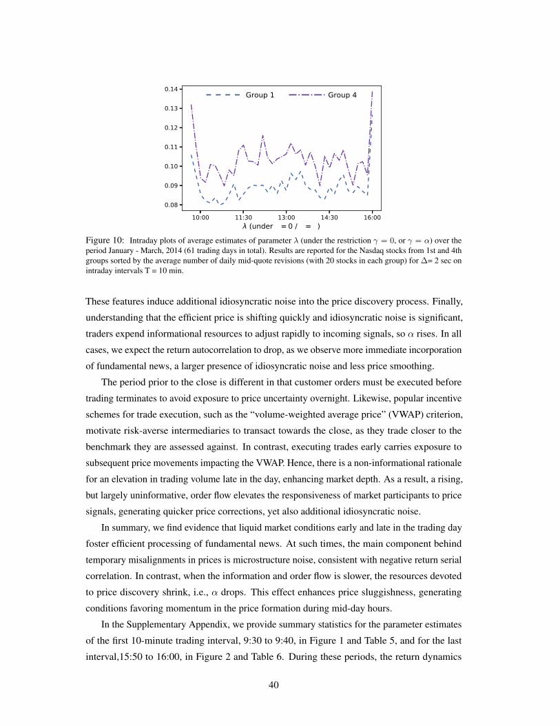
10:00 11:30 13:00 14:30 16:00λ (under γ=0 / γ=α)
0.08
0.09
0.10
0.11
0.12
0.13
0.14Group 1 Group 4
Figure 10: Intraday plots of average estimates of parameter λ (under the restriction γ = 0, or γ = α) over theperiod January - March, 2014 (61 trading days in total). Results are reported for the Nasdaq stocks from 1st and 4thgroups sorted by the average number of daily mid-quote revisions (with 20 stocks in each group) for ∆= 2 sec onintraday intervals T = 10 min.
These features induce additional idiosyncratic noise into the price discovery process. Finally,
understanding that the efficient price is shifting quickly and idiosyncratic noise is significant,
traders expend informational resources to adjust rapidly to incoming signals, so α rises. In all
cases, we expect the return autocorrelation to drop, as we observe more immediate incorporation
of fundamental news, a larger presence of idiosyncratic noise and less price smoothing.
The period prior to the close is different in that customer orders must be executed before
trading terminates to avoid exposure to price uncertainty overnight. Likewise, popular incentive
schemes for trade execution, such as the “volume-weighted average price” (VWAP) criterion,
motivate risk-averse intermediaries to transact towards the close, as they trade closer to the
benchmark they are assessed against. In contrast, executing trades early carries exposure to
subsequent price movements impacting the VWAP. Hence, there is a non-informational rationale
for an elevation in trading volume late in the day, enhancing market depth. As a result, a rising,
but largely uninformative, order flow elevates the responsiveness of market participants to price
signals, generating quicker price corrections, yet also additional idiosyncratic noise.
In summary, we find evidence that liquid market conditions early and late in the trading day
foster efficient processing of fundamental news. At such times, the main component behind
temporary misalignments in prices is microstructure noise, consistent with negative return serial
correlation. In contrast, when the information and order flow is slower, the resources devoted
to price discovery shrink, i.e., α drops. This effect enhances price sluggishness, generating
conditions favoring momentum in the price formation during mid-day hours.
In the Supplementary Appendix, we provide summary statistics for the parameter estimates
of the first 10-minute trading interval, 9:30 to 9:40, in Figure 1 and Table 5, and for the last
interval,15:50 to 16:00, in Figure 2 and Table 6. During these periods, the return dynamics
40

deviates substantially from the remainder of the trading day. We also report statistics across
all intraday intervals excluding the first and last 20 minutes of trading (Figure 3 and Table 7,
Supplementary Appendix). The latter confirm that the statistics reported in Figure 5 and Table
4 of the Supplementary Appendix are representative of the general market conditions and not
excessively distorted by the dynamics around the open and close.
5.4 Model-Implied versus Realized Return Volatility
As a final robustness check, we compare the relationship between the model-implied estimates
of the fundamental variance and realized volatility measures obtained at distinct frequencies.
This is useful to assess whether our 2-second sampling and stylized modeling generate biased
measures. The top panel of Figure 11 displays the average of the fundamental variance estimates
of σ2∗ along with the corresponding averages of daily realized volatility obtained from sampling
at the 2-second, 2- and 10-minute frequencies as well as from squared open-to-close returns.
By aggregating over the full sample period and all stocks, we should obtain reasonably precise
(average) volatility estimates from 10-minute sampling and squared open-to-close returns, while
one may suspect a bias in the standard RV measure based on 2-second returns and possibly also
from 2-minute sampling. The logic is similar to that of volatility signature plots, where the
average volatility may be approximated by averaging (nearly) unbiased, but noisy, estimates.
In fact, we find that both the averaged model-implied estimates and the 2-second average RV
measures generally are consistent with those obtained from 2-minute and 10-minute sampling
as well as with squared open-to-close returns. Upon closer inspection, there is a tendency
for the 2-second RV estimates to be a little below the other measures for liquidity groups 1-3
and higher for group 5. This is consistent with a minor average MMN bias in the 2-second
measure, where the more liquid stocks reveal more often positive return autocorrelations while
the illiquid stocks in group 5 experience more episodes with negative return autocorrelation.
This implies that RV measures tend to underestimate or overerestimate the underlying return
variation of the respective stocks, respectively.8 Nonetheless, the main impression is that all
these measures effectively are equivalent and point to no serious average biases even in the
2-second RV estimates. Importantly, the model-implied estimates are well aligned with the
robust estimates based on the 10-minute RV measure.
To further explore the properties of the model-implied volatility estimates, the middle and
bottom panels compare the model-implied estimate to the corresponding high-frequency based
RV measures for local windows with positive and negative return autocorrelations, respectively.
First, we confirm that the σ2∗ estimates consistently exceed the 2-second RV measure in the
8Given the very large number of observations, any visible differences in the bars are highly statistically significant.
41

1 2 3 4 50.0
0.1
0.2
0.3
0.4An
nual. v
olatilit
yAll intervals
Model-implied RV (2sec) RV (2min) RV (10min) Daily squared return
1 2 3 4 50.0
0.1
0.2
0.3
0.4
Annu
al. v
olatilit
y
Only intervals with non-negative return autocorrelationModel-implied RV (2sec) RV (2min) RV (10min)
1 2 3 4 5Liquidity groups
0.0
0.1
0.2
0.3
0.4
Annu
al. v
olatilit
y
Only intervals with negative return autocorrelationModel-implied RV (2sec) RV (2min) RV (10min)
Figure 11: The barplots show the average estimates of the return variance (represented in annualized volatilityunits) computed by the model-implied and several realized variance measures. The model-implied measures areestimates of the fundamental variance parameter σ2
∗ obtained from T = 10 min intervals sampled at frequency ∆= 2sec. The realized variance are computed at frequencies 2 sec, 2 min and 10 min. In addition, we consider the squaredopen-to-close return as a proxy for the daily return variance. All variance measures are averaged over the entireperiod (the first 61 trading days in 2014) and over the stocks of a given liquidity group, where groups are sorted bythe average number of daily mid-quote revisions (20 stocks per group).
middle panel and fall below the 2-second RV measure in the bottom panel. This is a largely
mechanical result, as our model translates the estimated second order return moments into
structural parameters that interpret the autocorrelation as signals of distortions induced by MMN
in line with the directional effects observed in the two bottom panels. More interestingly, we
observe the identical general directional association between the model-implied estimates and
42

the RV measures based on more sparsely sampled returns. I.e., the average σ2∗ estimate exceeds
all RV measures in the middle panel and is below all RV measures in the bottom panel. This is
consistent with the MMN induced autocorrelation structure estimated from 2-second frequency
implying similar effects for the 2- and 10-minute frequencies and generating biases over the full
length windows of 10 minutes.
To summarize, our microstructure model estimated over short intraday intervals generally
produces return variation estimates that are consistent with those obtained from standard realized
volatility measures. However, they also deviate systematically, whenever there is notable
autocorrelation in the very high-frequency return series. This corroborates the hypothesis that
sizable MMN effects generate biases in realized volatility estimates of varying sign. For longer
periods, like a full trading day, such effects are often mitigated by cancellations induced by
the shifting signs of the bias, yet it remains non-trivial over shorter time windows and it will
manifest itself significantly for days where the predominant MMN features induce persistent
spells of return serial dependence of a given sign. As such, our empirical results bridge the
MMN and RV literatures: the main microstructure theories imply a form for noise endogeneity
that violates the standard infill asymptotic RV approach, while the RV measures are robust to
strongly time-varying heteroskedasticity in the return series of a type that is absent in popular
microstructure models. By focusing on a simple structural model, estimated over short windows
to accommodate the time-varying features of the return process, we generally obtain consistent
return variation measures, but also strong evidence that the MMN effects biases the RV measures
in specific directions during episodes when the prevailing market conditions induce persistent
return autocorrelation patterns.
6 Concluding Remarks
MMN leaves a distinct imprint on high-frequency financial returns, manifesting itself through
(absolute) return autocorrelations for individual stocks which (i) are highly significant, on
average, over local intervals, and (ii) display persistence, yet also undergoes rapidly shifting
signs. The fact that a large proportion of local intervals display a nontrivial degree of positive
return autocorrelation is a new finding, contradicting the common assumption of MMN as
being exogenous to the efficient price process. Notably, exogeneity is also inconsistent with
well-known market microstructure models, such as Glosten and Milgrom (1985) suggesting that
price discovery and noise innovations are intrinsically related, and Kyle (1985) or Vives (1995),
who points towards longer-lasting pricing errors induced by strategic trading and learning.
Consequently, the portrayals of the price formation process in the market microstructure lit-
erature are at odds with the econometric literature on high-frequency based volatility estimation.
43

Specifically, realized volatility measures usually rely on “semimartingale-plus-noise” models,
precluding persistent structural interactions between the efficient price innovations and noise.
Instead, the key assumption is that the noise component becomes dominant, and thus locally
identifiable by nonparametric means, as the sampling interval shrinks to zero. This defies the
idea of significant longer-run dependencies in the error process itself and for its interaction with
the fundamental price innovations.
We seek to bridge this gap by extending the martingale-plus-noise model so that it aligns
better with the structural market microstructure literature and the empirical footprint left by
MMN through the high-frequency return autocorrelogram. Our modification introduces noise
endogeneity and an error correction mechanism capturing partial adjustment dynamics along
the lines of Amihud and Mendelson (1987). This parsimonious reduced-form model captures
the salient features of the high-frequency return dynamics for local intervals. The interplay
of the model’s four parameters - the volatility of the underlying martingale process, the noise
variance, the strength of temporal error correction, and the correlation, or endogeneity, between
the efficient price innovations and noise - triggers local intervals of ’momentum’ behavior
(positive autocorrelations) and ’contrarian’ trading (negative autocorrelations). Moreover, it
helps to identify the complementary roles of the temporal error correction component and the
endogenous pricing errors in determining the sign and strength of the return autocorrelations.
An immediate consequence of an error correction component, rationalized by learning and
delayed information processing, is that the (calendar) time correlation pattern itself becomes
an integral part of the model specification. As a result, the model is naturally cast in discrete
time, rather than as a continuous-time diffusion system involving vanishing dependency as the
sampling intervals shrinks in accordance with an infill asymptotic setting.
We hasten to add that, unquestionable, the realized volatility approach has drastically
improved our ability to monitor and model the evolving return variation process. The point is
that daily realized volatility measures are largely unaffected by such local biases, as long as the
positive and negative autocorrelation regimes are evenly balanced across the trading day, and
thus cancel through intertemporal averaging. Nonetheless, it does imply that local realized (spot)
volatility estimates are subject to potentially significant biases. Moreover, trading days for which
the return autocorrelation pattern is highly one-sided will be associated with realized volatility
measures that are subject to a substantial measurement error. A few concurrent papers deal
with extreme manifestations of this phenomenon, in the sense that they identify individual local
episodes of highly significant semimartingale violations, which warrant separate interpretation
and treatment, see, e.g., Christensen et al. (2018) and Andersen et al. (2019). An earlier piece
noting the need for filtering episodes featuring unusually strong return serial correlation is
Barndorff-Nielsen et al. (2008a), who classified such episodes as “sliding jumps.”
44
We differ from the studies above by documenting that local violations of the semimartingale
hypothesis are common, yet also fleeting, and we link this observation to the constant arrival
of economic news in the presence of incomplete and asymmetric information, ongoing price
discovery and learning, noise, and trading costs. Specifically, using high-frequency mid-quote
returns from Nasdaq, we find that a flexible price discovery process in line with our information
delay model is useful for capturing the high-frequency return dynamics over local intervals. We
show that the pricing error is endogenous and, consequently, the classic martingale-plus-iid-
noise model is rejected. Moreover, the incorporation of a sluggish price adjustment is critical
for modeling the dynamics of high-frequency returns.
From a statistical viewpoint, this paper makes a number of contributions. First, the proposed
model provides a more structural treatment of market microstructure noise capturing sources of
endogeneity and temporal dependence. These insights can be exploited to construct conceptually
novel model-based estimators of volatility that adapt more explicitly to this noise structure.
Second, we show that even minor extensions of the martingale-plus-noise model may not be fully
identifiable. In particular, the signal-to-noise ratio is only partially identified if the covariance
between the MMN and efficient price components are unconstrained. We accommodate the
partial identification feature through restrictions on the parameter space for which we conduct
inference. It also implies an observational equivalence between an error correction mechanism
based on the current (efficient) price (Amihud and Mendelson (1987)) and temporal corrections
of mispricing based on the lagged efficient price (”information delay model”). Nonetheless,
the fundamental volatility estimator is always fully identified in these settings. Third, our
results provide strong evidence for locally shifting return dynamics. These findings have direct
implications for local volatility estimation and should, in periods with unusual return dynamics,
also help mitigate biases associated with the estimation of volatility over longer daily or weekly
horizons. In summary, the combination of market microstructure inspired modeling and explicit
recognition of the ever evolving market dynamics opens up interesting avenues for future work
on the construction of alternative local and daily volatility estimators.
References
AIT-SAHALIA, Y. AND J. JACOD (2014): High-Frequency Financial Econometrics, Princeton University Press.
AIT-SAHALIA, Y., P. MYKLAND, AND L. ZHANG (2005): “How Often to Sample a Continuous-Time Process in
the Presence of Market Microstructure Noise,” Review of Financial Studies, 351–416.
——— (2006): “Comment,” Journal of Business & Economic Statistics, 162–167.
AMIHUD, Y. AND H. MENDELSON (1987): “Trading Mechanisms and Stock Returns: An Empirical Investigation,”
Journal of Finance, 42 (3), 533–553.
45

ANDERSEN, T. G. AND T. BOLLERSLEV (1998): “Answering the Skeptics: Yes, Standard Volatility Models Do
Provide Accurate Forecasts,” International Economic Review, 39, 885–905.
——— (2018a): “Introduction,” in Volatility, Volume I, ed. by T. G. Andersen and T. Bollerslev, Cheltenham, U.K.;
Northampton, MA, U.S.: Edward Elgar Publishing, xiii–xli.
——— (2018b): Volatility, Volume I and II, Edward Elgar Publishing.
ANDERSEN, T. G., T. BOLLERSLEV, F. DIEBOLD, AND P. LABYS (2003): “Modeling and Forecasting Realized
Volatility,” Econometrica, 71, 579–625.
ANDERSEN, T. G., Y. LI, V. TODOROV, AND B. ZHOU (2019): “Black Holes in High-Frequency Financial Data,”
Working Paper, Hong Kong UST and Northwestern University.
BANDI, F. AND J. RUSSELL (2006): “Separating Microstructure Noise from Volatility,” Journal of Financial
Economics, 79, 655–692.
——— (2008): “Microstructure Noise, Realized Variance, and Optimal Sampling,” Review of Economic Studies, 75,
339–369.
BARNDORFF-NIELSEN, O. E., P. HANSEN, A. LUNDE, AND N. SHEPHARD (2008a): “Realised Kernels in Practice:
Trades and Quotes,” Econometrics Journal, 4, 1–32.
BARNDORFF-NIELSEN, O. E., P. R. HANSEN, A. LUNDE, AND N. SHEPHARD (2008b): “Designing Realized
Kernels to Measure the ex post Variation of Equity Prices in the Presence of Noise,” Econometrica, 76, 1481–1536.
BIBINGER, M., N. HAUTSCH, P. MALEC, AND M. REISS (2014): “Estimating the quadratic covariation matrix
from noisy observations: local method of moments and efficiency,” Annals of Statistics, 42, 1312–1364.
CHAKER, S. (2013): “Volatility and Liquidity Costs,” Tech. Rep. 2013-29, Bank of Canada.
CHRISTENSEN, K., R. OOMEN, AND R. RENO (2018): “The drift burst hypothesis,” Working Paper, University of
Aarhus.
DA, R. AND D. XIU (2019): “When Moving Average Models Meet High-Frequency Data: Uniform Inference on
Volatility,” Working Paper, University of Chicago.
DIEBOLD, F. AND G. STRASSER (2013): “On the Correlation Structure of Microstructure Noise: A Financial
Economic Approach,” Review of Economic Studies, 80, 1304–1337.
GLOSTEN, L. AND P. MILGROM (1985): “Bid, Ask and Transaction Prices in a Specialist Market with Heteroge-
neously Informed Traders,” Journal of Financial Markets Economics, 14, 71–100.
GONCALVES, S. AND N. MEDDAHI (2009): “Bootstrapping Realized Volatility,” Econometrica, 77, 283–306.
HANSEN, P. R. AND A. LUNDE (2006): “Realized Variance and Market Microstructure Noise,” Journal of Business
and Economic Statistics, 24, 127–161.
HARVEY, A. C. (1989): Forecasting. Structural Time Series Models and the Kalman Filter., Cambridge University
Press.
46
HASBROUCK, J. AND T. HO (1987): “Order Arrival, Quote Behavior, and the Return-Generating Process,” Journal
of Finance, 42, 1035–1048.
HOLDEN, C. AND A. SUBRAHMANYAM (1992): “Long-Lived Private Information and Imperfect Competition,”
Journal of Finance, 47, 247–270.
——— (1996): “Risk Aversion, Liquidity, and Endogenous Short Horizons,” Review of Financial Studies, 9,
691–722.
HUANG, X. AND G. TAUCHEN (2005): “The Relative Contribution of Jumps to Total Price Variance,” Journal of
Financial Econometrics, 3, 456–499.
JACOD, J., Y. LI, P. MYKLAND, M. PODOLSKIJ, AND M. VETTER (2009): “Mirostructure noise in the continuous
case: the pre-averaging approach,” Stochastic Processes and Their Applications, 26, 2803–2831.
JACOD, J., Y. LI, AND X. ZHENG (2017): “Statistical Properties of Microstructure Noise,” Econometrica, 85,
1133–1174.
KALNINA, I. AND O. LINTON (2008): “Estimating Quadratic Variation Consistently in the Presence of Endogenous
and Diurnal Measurement Error,” Journal of Econometrics, 147, 47–59.
KOKOSZKA, P. AND D. POLITIS (2011): “Non-linearity of ARCH and stochastic volatility models and Bartlett’s
formula,” Probability and Mathematical Statistics, 31, 47–59.
KYLE, A. S. (1985): “Continuous Auctions and Insider Trading,” Econometrica, 53 (6), 1315–1335.
LI, Y., S. XIE, AND X. ZHENG (2016): “Efficient Estimation of Integrated Volatility Incorporating Trading
Information,” Tech. rep., Hong Kong University of Science and Technology.
LI, Z. AND O. LINTON (2016): “Robust Measures of Microstructure Noise,” Tech. rep., Hong Kong University of
Science and Technology.
MADHAVAN, A., M. RICHARDSON, AND M. ROOMANS (1997): “Why Do Security Prices Change? A Transaction-
Level Analysis of NYSE Stocks,” Review of Financial Studies, 10, 1035–1064.
MYKLAND, P. AND L. ZHANG (2009): “Inference for Continuous Semimartingales Observed at High Frequency,”
Econometrica, 77, 1403–1445.
ROLL, R. (1984): “A Simple Implicit Measure of the Effective Bid-Ask Spread in an Efficient Market,” Journal of
Finance, 1127–1140.
SHEPPARD, K. (2013): “Measuring Market Speed,” Tech. rep., University of Oxford.
VIVES, X. (1995): “The Speed of Information Revelation in a Financial Market Mechanism,” Journal of Economic
Theory, 67, 187–204.
ZHANG, L., P. MYKLAND, AND Y. AIT-SAHALIA (2005): “A Tale of Two Time Scales: Determining Integrated
Volatility With Noisy High-Frequency Data,” Journal of the American Statistical Association, 100, 13941411.
ZHOU, B. (1996): “High-Frequency Data and Volatility in Foreign-Exchange Rates,” Journal of Business and
Economic Statistics, 45–52.
47