Local helioseismology using ring diagram analysis

Astron. Nachr. / AN 328, No. 3/4, 257 – 263 (2007) / DOI 10.1002/asna.200610727

Local helioseismology using ring diagram analysis

H.M. Antia1,� and S. Basu2

1 Tata Institute of Fundamental Research, Homi Bhabha Road, Mumbai 400005, India2 Astronomy Department, Yale University, P. O. Box 208101, New haven CT 06520-8101, U. S. A.

Received 2006 Nov 17 , accepted 2007 Jan 2

Published online 2007 Feb 28

Key words Sun: helioseismology – Sun: oscillations – Sun: interior

Ring diagram analysis is an extension of global helioseismology that is applied to small areas on the Sun. It can be used toinfer the horizontal components of large scale flows as well as the structure, and variations thereof, in the outer convectionzone. We describe below the ring-diagram analysis technique, and some results obtained using this technique.

c© 2007 WILEY-VCH Verlag GmbH & Co. KGaA, Weinheim

1 Introduction

Helioseismology has successfully determined the solar in-

ternal structure (e.g., Gough et al. 1996) as well as the ro-

tation rate in the solar interior (e.g., Thompson et al. 1996;

Schou et al. 1998). However, the low and intermediate de-

gree modes that are used in these global studies do not re-

solve features near the solar surface adequately. Further-

more, the global modes are only sensitive to the east-west

component of horizontal velocity (i.e. rotation). And these

modes are only sensitive to the longitudinally-averaged

north-south symmetric component of the rotation rate and

of structure. The meridional (north-south) component of

velocity cannot be studied using the global modes. Lo-

cal helioseismic techniques need to be employed to study

the meridional component of velocity as well as to study

the longitudinal variation of solar flows and solar struc-

ture. These techniques, which are effectively based on high-

degree modes of solar oscillations, also give better resolu-

tion near the solar surface when compared to global tech-

niques.

High-degree solar oscillation modes (� ≥ 150) which

are trapped in the outer parts of the solar envelope have

lifetimes that are much smaller than the sound travel time

around the Sun and hence the characteristics of these modes

are mainly determined by average conditions in the local

neighbourhood rather than the average conditions over the

entire spherical shell. The properties of these modes are

better determined by local helioseismic techniques. Ring

diagram (plane wave k-ν) analysis (Hill 1988) and time-

distance analysis (Duvall et al. 1993) are examples of such

local helioseismic techniques. In this review we will de-

scribe only the ring-diagram analysis. For other techniques

readers can refer to Gizon & Birch (2005) and other articles

in this issue.

� Corresponding author: [email protected]

Ring diagram analysis is an extension of global helio-

seismic analysis with the observations being restricted to a

small region (typically 15◦×15◦) of the solar surface. Ring

diagrams are obtained from a time series of Dopplergrams

of a specific area of the Sun generally tracked with the mean

rotation velocity. The Dopplergrams are remapped to helio-

graphic co-ordinates while tracking. The three dimensional

Fourier transform of this time series gives the power spec-

trum P (kx, ky, ν), where kx, ky are the wavenumbers in the

two spatial directions and ν is the cyclic frequency. These

power spectra are referred to as ring diagrams because of

the characteristic ring-like shape of regions where the power

is concentrated in sections of constant temporal frequency,

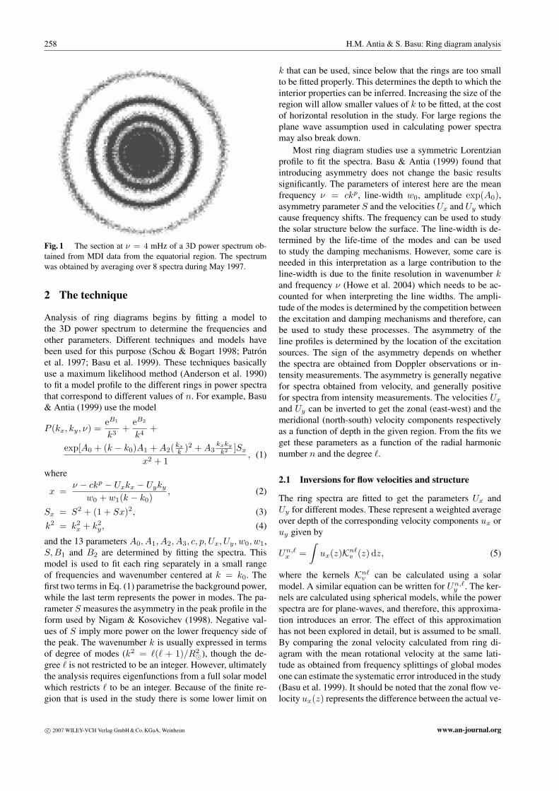
reflecting the near azimuthal symmetry of the power in kspace (Fig. 1).

These 3D power spectra are the basic inputs for ring dia-

gram analysis. The frequency ν(kx, ky) where the power is

concentrated provides the diagnostic for the region studied.

In particular, these frequencies are shifted due to flows in the

horizontal (x, i.e., zonal, and y, i.e., meridional) directions.

By measuring the frequency shifts one can, in principle, es-

timate the flow velocities below the surface. The frequency

shifts and other parameters are a horizontal average of these

parameters over the region studied. Thus the size of the cho-

sen region determines the spatial resolution of ring diagram

studies. This size in turn, is determined by the necessity of

being able to resolve modes with different wavenumbers

in some suitable range. For the spatial resolution of MDI

(Michelson Doppler Imager) and GONG (Global Oscilla-

tions Network Group) instruments a size of 15◦ × 15◦ is

found to be reasonable for most applications.

In the next section we describe the technique used in fit-

ting the ring diagram power spectra and the inversion tech-

niques to infer the flows and structure variations. In Sec. 3,

we describe some of the results that have been obtained us-

ing this technique.

c© 2007 WILEY-VCH Verlag GmbH & Co. KGaA, Weinheim

258 H.M. Antia & S. Basu: Ring diagram analysis

Fig. 1 The section at ν = 4 mHz of a 3D power spectrum ob-

tained from MDI data from the equatorial region. The spectrum

was obtained by averaging over 8 spectra during May 1997.

2 The technique

Analysis of ring diagrams begins by fitting a model to

the 3D power spectrum to determine the frequencies and

other parameters. Different techniques and models have

been used for this purpose (Schou & Bogart 1998; Patron

et al. 1997; Basu et al. 1999). These techniques basically

use a maximum likelihood method (Anderson et al. 1990)

to fit a model profile to the different rings in power spectra

that correspond to different values of n. For example, Basu

& Antia (1999) use the model

P (kx, ky, ν) =eB1

k3+

eB2

k4+

exp[A0 + (k − k0)A1 + A2(kx

k )2 + A3kxky

k2 ]Sx

x2 + 1, (1)

where

x =ν − ckp − Uxkx − Uyky

w0 + w1(k − k0), (2)

Sx = S2 + (1 + Sx)2, (3)

k2 = k2x + k2

y, (4)

and the 13 parameters A0, A1, A2, A3, c, p, Ux, Uy, w0, w1,

S,B1 and B2 are determined by fitting the spectra. This

model is used to fit each ring separately in a small range

of frequencies and wavenumber centered at k = k0. The

first two terms in Eq. (1) parametrise the background power,

while the last term represents the power in modes. The pa-

rameter S measures the asymmetry in the peak profile in the

form used by Nigam & Kosovichev (1998). Negative val-

ues of S imply more power on the lower frequency side of

the peak. The wavenumber k is usually expressed in terms

of degree of modes (k2 = �(� + 1)/R2�), though the de-

gree � is not restricted to be an integer. However, ultimately

the analysis requires eigenfunctions from a full solar model

which restricts � to be an integer. Because of the finite re-

gion that is used in the study there is some lower limit on

k that can be used, since below that the rings are too small

to be fitted properly. This determines the depth to which the

interior properties can be inferred. Increasing the size of the

region will allow smaller values of k to be fitted, at the cost

of horizontal resolution in the study. For large regions the

plane wave assumption used in calculating power spectra

may also break down.

Most ring diagram studies use a symmetric Lorentzian

profile to fit the spectra. Basu & Antia (1999) found that

introducing asymmetry does not change the basic results

significantly. The parameters of interest here are the mean

frequency ν = ckp, line-width w0, amplitude exp(A0),asymmetry parameter S and the velocities Ux and Uy which

cause frequency shifts. The frequency can be used to study

the solar structure below the surface. The line-width is de-

termined by the life-time of the modes and can be used

to study the damping mechanisms. However, some care is

needed in this interpretation as a large contribution to the

line-width is due to the finite resolution in wavenumber kand frequency ν (Howe et al. 2004) which needs to be ac-

counted for when interpreting the line widths. The ampli-

tude of the modes is determined by the competition between

the excitation and damping mechanisms and therefore, can

be used to study these processes. The asymmetry of the

line profiles is determined by the location of the excitation

sources. The sign of the asymmetry depends on whether

the spectra are obtained from Doppler observations or in-

tensity measurements. The asymmetry is generally negative

for spectra obtained from velocity, and generally positive

for spectra from intensity measurements. The velocities Ux

and Uy can be inverted to get the zonal (east-west) and the

meridional (north-south) velocity components respectively

as a function of depth in the given region. From the fits we

get these parameters as a function of the radial harmonic

number n and the degree �.

2.1 Inversions for flow velocities and structure

The ring spectra are fitted to get the parameters Ux and

Uy for different modes. These represent a weighted average

over depth of the corresponding velocity components ux or

uy given by

Un,�x =

∫ux(z)Kn�

v (z) dz, (5)

where the kernels Kn�v can be calculated using a solar

model. A similar equation can be written for Un,�y . The ker-

nels are calculated using spherical models, while the power

spectra are for plane-waves, and therefore, this approxima-

tion introduces an error. The effect of this approximation

has not been explored in detail, but is assumed to be small.

By comparing the zonal velocity calculated from ring di-

agram with the mean rotational velocity at the same lati-

tude as obtained from frequency splittings of global modes

one can estimate the systematic error introduced in the study

(Basu et al. 1999). It should be noted that the zonal flow ve-

locity ux(z) represents the difference between the actual ve-

c© 2007 WILEY-VCH Verlag GmbH & Co. KGaA, Weinheim www.an-journal.org

Astron. Nachr. / AN (2007) 259

locity and the mean rotation velocity assumed while track-

ing the region.

Equation (5) defines a linear inverse problem to deter-

mine the velocity ux(z) (or uy(z)) when the kernels and

Un,�x (or Un,�

y ) are known for a set of modes. This is ba-

sically an ill-conditioned problem and we need some addi-

tional assumptions to get a reasonable solution. This is gen-

erally done by assuming that the solution is smooth in some

sense. There are many techniques for solving inverse prob-

lems (Gough & Thompson 1991). The two main approaches

are the Regularised Least Squares (RLS) and the Optimally

Localised Averages (OLA) methods.

The basic idea of the RLS method is to expand the re-

quired solution in terms of suitable basis functions and to

determine the coefficients of expansion by minimising the

sum of the squared differences between the observations

and the adopted model. An additional term is added to en-

sure smoothness of the solution. This is usually the integral

of the squared second derivative. For example, we minimise

a function of the form

χ2 =∑n,�

1σ2

n,�

(Un,�

x −∫

Kn,�v (z)ux(z) dz

)2

+ λ

∫ (d2ux(z)

dz2

)2

dz . (6)

Here we have assumed the errors, σn,� to be independent

of each other. The constant λ is a regularisation parameter,

which is adjusted to get appropriate smoothness of the solu-

tion. If λ = 0, the solution reduces to a normal least squares

approximation, while for very large values of λ the solution

will approach a linear function. In particular, at large depths

where only a few modes penetrate, the resulting solution

will tend to be linear. For the second term of Eq. (6) we can

choose to minimise the first derivative instead of the second

derivative. In that case the solution will approach a constant

value as λ → ∞. The choice of λ is arbitrary to some ex-

tent, but it can be selected by experimenting with artificial

data calculated for known velocity profiles with random er-

rors (consistent with those in the observed data) added to

the artificial data. The inversion results for these artificial

data can then be compared with the known input profiles to

estimate an optimal value of λ. If λ is properly chosen then

the results are not very sensitive to small variations in this

parameter.

The OLA technique (Backus & Gilbert 1968) attempts

to produce a linear combination of data such that the result-

ing averaging kernel is suitably localised while simultane-

ously controlling the error estimates. The basic idea in OLA

method is to construct a linear combination of data,

ux(z0) =∑n,�

an,�(z0)Un,�x =

∫K(z, z0)ux(z) dz, (7)

where K(z, z0) is the averaging kernel given by

K(z, z0) =∑n,�

an,�(z0)Kn,�v (z) . (8)

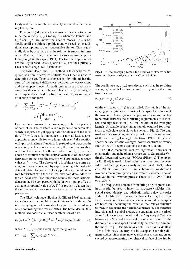
Fig. 2 A few averaging kernels for inversion of flow velocities

from ring diagram analysis using the OLA technique.

The coefficients an,�(z0) are selected such that the resulting

averaging kernel is localised around z = z0 and at the same

time the error

σ2ux

(z0) =∑n,�

a2n,�(z0)σ2

n,� (9)

on the estimated ux(z0) is controlled. The width of the av-

eraging kernel gives an estimate of the spatial resolution of

the inversion. Once again an appropriate compromise has

to be made between the conflicting requirements of low er-

rors and high resolution (i.e., small width) of the averaging

kernels. A sample of averaging kernels obtained for inver-

sions to calculate solar flows is shown in Fig. 2. The data

used are for a ring diagram analysis of the equatorial region

of the Sun during Carrington Rotation 1910. The power-

spectrum used was the averaged power spectrum of twenty

four 15◦ × 15◦ regions spanning the entire rotation.

The OLA technique requires significant amounts of

computation and quite often a variant called Subtractive Op-

timally Localised Averages (SOLA) (Pijpers & Thompson

1992, 1994) is used. These techniques have been success-

fully used for ring diagram analysis (Basu et al. 1999; Haber

et al. 2002). Comparison of results obtained using different

inversion techniques gives an estimate of systematic errors

involved in the inversion process (Basu et al. 1999; Haber

et al. 2004).

The frequencies obtained from fitting ring diagrams can,

in principle, be used to invert for structure variables like,

sound speed, density and adiabatic index below the solar

surface. Unlike the inversion for flow velocities, the inver-

sion for structure variations is nonlinear and all techniques

are based on linearising the equation that relates structure

to frequencies using the variational principle. For structure

inversions using global modes, the equations are linearised

around a known solar model, and the frequency differences

between the Sun and the model are inverted to obtain the

difference in sound speed and density between the Sun and

the model (e.g., Dziembowski et al. 1990; Antia & Basu

1994). This however, may not be acceptable for ring dia-

gram studies, since there may be unknown systematic errors

caused by approximating the spherical surface of the Sun by

www.an-journal.org c© 2007 WILEY-VCH Verlag GmbH & Co. KGaA, Weinheim


a plane-parallel model as well as those caused by the pro-

jection of a spherical surface onto a plane, particularly at

high latitudes. As a result, in most ring diagram studies of

solar structure, we take the differences between two sets of

observed frequencies to study the differences in structure

between the corresponding regions. If these structural dif-

ferences are small, the linearisation may be justified. Thus

the difference in frequencies of two regions would be re-

lated by

δνn,�

νn,�=

∫Kn,�

c,ρ (z)δc2

c2(z) dz

+∫

Kn,�ρ,c (z)

δρ

ρ(z) dz +

F (νn,�)In,�

. (10)

Here again the kernels can be calculated from a known so-

lar model. The kernel Kc,ρ(z) measures the sensitivity of

frequencies to variations in sound speed at constant den-

sity, while Kρ,c(z) measures the effect of density at con-

stant sound speed. The function F (ν) is a smooth function

which takes into account uncertainties in layers very close

to the surface, while In,� is the mode inertia. This term is es-

sentially ad hoc and takes account of various contributions

from near-surface layers, such as non-adiabatic effects, that

are not included in the variational principle. In addition to

ignored effects, the surface term also accounts for contribu-

tions from near-surface regions that cannot be resolved by

the mode set used for the inversions. Once again we can use

any of the inversion techniques like RLS, OLA or SOLA for

calculating the structure difference between two regions in

the Sun (e.g., Basu et al. 2004).

3 Results

Ring diagram analysis was proposed by Hill (1988) for

studying flows in the solar interior. Hill (1989) used data

obtained at NSO to study the flow velocities in four dif-

ferent regions on the Sun and found variations of order

of 20 m s−1. Subsequently, Hill (1990) applied inversion

techniques to infer the flow velocities as a function of the

depth from frequency shifts caused by flows. The shifts

were determined by fitting ellipses to the rings at constant

frequency. Patron et al. (1997) attempted to fit 3D power

spectra using a Lorentzian profile, and applied this to data

obtained from the Taiwan Oscillation Network (TON). With

the availability of data from the MDI instrument on board

SOHO, considerable progress has been made in applying

ring diagram technique to study large scale flows in the solar

interior. The updated GONG instruments are now providing

near-continuous coverage of the Sun, and the data are being

successfully used for ring-diagram analysis.

Although ring diagram analysis cannot measure the flow

velocities in the vertical direction, Komm et al. (2004) have

attempted to use the continuity equation to estimate the ver-

tical component using the horizontal velocities on a grid of

regions covering the solar surface. Considering the low res-

olution of ring diagram technique and significant uncertain-

ties in the horizontal velocities, it is not clear if such efforts

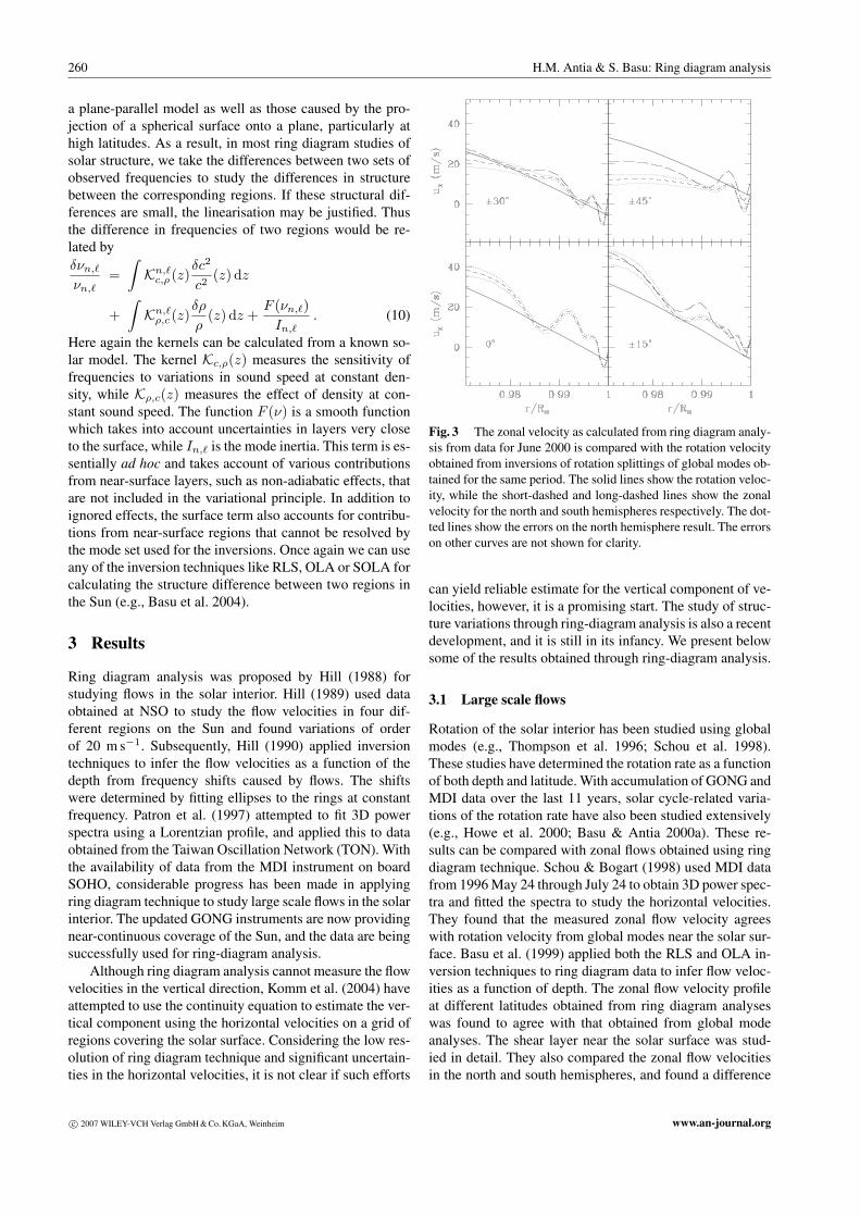
Fig. 3 The zonal velocity as calculated from ring diagram analy-

sis from data for June 2000 is compared with the rotation velocity

obtained from inversions of rotation splittings of global modes ob-

tained for the same period. The solid lines show the rotation veloc-

ity, while the short-dashed and long-dashed lines show the zonal

velocity for the north and south hemispheres respectively. The dot-

ted lines show the errors on the north hemisphere result. The errors

on other curves are not shown for clarity.

can yield reliable estimate for the vertical component of ve-

locities, however, it is a promising start. The study of struc-

ture variations through ring-diagram analysis is also a recent

development, and it is still in its infancy. We present below

some of the results obtained through ring-diagram analysis.

3.1 Large scale flows

Rotation of the solar interior has been studied using global

modes (e.g., Thompson et al. 1996; Schou et al. 1998).

These studies have determined the rotation rate as a function

of both depth and latitude. With accumulation of GONG and

MDI data over the last 11 years, solar cycle-related varia-

tions of the rotation rate have also been studied extensively

(e.g., Howe et al. 2000; Basu & Antia 2000a). These re-

sults can be compared with zonal flows obtained using ring

diagram technique. Schou & Bogart (1998) used MDI data

from 1996 May 24 through July 24 to obtain 3D power spec-

tra and fitted the spectra to study the horizontal velocities.

They found that the measured zonal flow velocity agrees

with rotation velocity from global modes near the solar sur-

face. Basu et al. (1999) applied both the RLS and OLA in-

version techniques to ring diagram data to infer flow veloc-

ities as a function of depth. The zonal flow velocity profile

at different latitudes obtained from ring diagram analyses

was found to agree with that obtained from global mode

analyses. The shear layer near the solar surface was stud-

ied in detail. They also compared the zonal flow velocities

in the north and south hemispheres, and found a difference



of about 5 m s−1 near the surface, but in view of possible

systematic errors it is not clear if this can be considered to

be significant. Similar results were obtained by Gonzalez

Hernandez & Patron (2000). Figure 3 shows a comparison

of zonal velocities in the two hemispheres obtained by ring

diagram analysis with rotation velocity inferred from rota-

tional splittings of global modes. While Basu et al. (1999)

studied ring spectra at different latitudes that were aver-

aged over an entire Carrington rotation to improve preci-

sion, Haber et al. (2000) used ring diagram analysis to study

mosaics of regions covering entire solar surface up to a lat-

itude of 60◦ (usually referred to as the ‘dense-pack’) at dif-

ferent times. They used this to study the variation in flow

velocities over latitude and longitude.

Haber et al. (2000) and Basu & Antia (2000b) have iden-

tified the torsional oscillation pattern in the east-west flows.

A similar pattern of temporal variation has been seen at the

solar surface (Howard & LaBonte 1980) and in the inte-

rior using global modes (Howe et al. 2000; Basu & Antia

2000a). Haber et al. (2000) also found north-south asym-

metry in the zonal flow velocities. Some north-south asym-

metry has been found in all results, but there is no agreement

between different results and it is not clear if there is indeed

any significant asymmetry.

Unlike zonal flows, meridional flows cannot be deter-

mined from frequency splittings of global modes, and hence

these have been inferred using local helioseismic techniques

only. Surface Doppler measurements have shown merid-

ional flows with an amplitude of about 27 m s−1 from the

equator to the poles in both hemispheres (e.g., Hathaway et

al. 1996). These flows play a crucial role in modern solar dy-

namo theories (e.g., Dikpati & Charbonneau 1999; Nandy

& Choudhuri 2002), and hence it is important to study these

flows in the solar interior. In particular, conservation of mass

requires that the direction of meridional flow should reverse

below some depth in the interior. Many dynamo models

assume that this occurs around the tachocline, but current

helioseismic technique cannot give any information about

these flows at such depths.

Giles et al. (1997) were the first to detect meridional

flows in the solar interior using time-distance technique.

Their results agree with those obtained using ring diagram

analysis (Schou & Bogart 1998; Basu et al. 1999; Gonzalez

Hernandez et al. 1999; Haber et al. 2000). These studies

did not find any evidence of a return flow from the poles

to the equator up to a depth of about 21 Mm–ring-diagram

analyses cannot probe deeper layers. The dominant compo-

nent of the meridional flow has a form vm sin 2θ, where θis the colatitude and the amplitude is found to be about 30

m s−1 near the surface. There is only a weak depth depen-

dence in the amplitude of this component. Higher compo-

nents are also significant at intermediate depths. In partic-

ular, the component P 14 (cos θ) (where Pm

� (x) is the asso-

ciated Legendre polynomial) suggested by Durney (1993)

is found to have an amplitude of about 3–4 m s−1 (Basu et

al. 1999; Basu & Antia 2003). The north-south symmetric

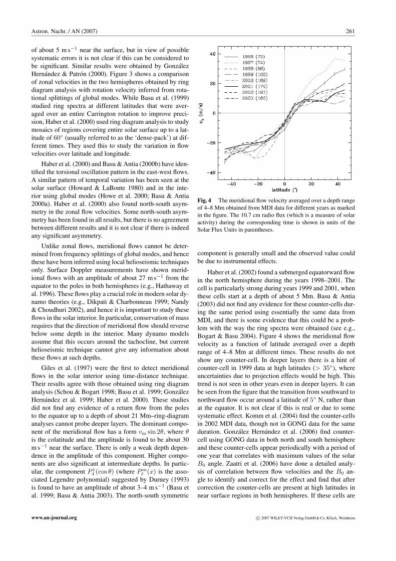
Fig. 4 The meridional flow velocity averaged over a depth range

of 4–8 Mm obtained from MDI data for different years as marked

in the figure. The 10.7 cm radio flux (which is a measure of solar

activity) during the corresponding time is shown in units of the

Solar Flux Units in parentheses.

component is generally small and the observed value could

be due to instrumental effects.

Haber et al. (2002) found a submerged equatorward flow

in the north hemisphere during the years 1998–2001. The

cell is particularly strong during years 1999 and 2001, when

these cells start at a depth of about 5 Mm. Basu & Antia

(2003) did not find any evidence for these counter-cells dur-

ing the same period using essentially the same data from

MDI, and there is some evidence that this could be a prob-

lem with the way the ring spectra were obtained (see e.g.,

Bogart & Basu 2004). Figure 4 shows the meridional flow

velocity as a function of latitude averaged over a depth

range of 4–8 Mm at different times. These results do not

show any counter-cell. In deeper layers there is a hint of

counter-cell in 1999 data at high latitudes (> 35◦), where

uncertainties due to projection effects would be high. This

trend is not seen in other years even in deeper layers. It can

be seen from the figure that the transition from southward to

northward flow occur around a latitude of 5◦ N, rather than

at the equator. It is not clear if this is real or due to some

systematic effect. Komm et al. (2004) find the counter-cells

in 2002 MDI data, though not in GONG data for the same

duration. Gonzalez Hernandez et al. (2006) find counter-

cell using GONG data in both north and south hemisphere

and these counter-cells appear periodically with a period of

one year that correlates with maximum values of the solar

B0 angle. Zaatri et al. (2006) have done a detailed analy-

sis of correlation between flow velocities and the B0 an-

gle to identify and correct for the effect and find that after

correction the counter-cells are present at high latitudes in

near surface regions in both hemispheres. If these cells are



real they will have consequences for the angular momentum

transport as well as solar dynamo theories. More studies are

needed to confirm or reject the existence of these cells. In

addition to the counter-cell, other temporal variations have

also been seen when the meridional flow pattern is aver-

aged over an entire solar rotation. These variations can be

studied using the residuals obtained by subtracting tempo-

ral averages from the observed values at each latitude. These

residues are found to be of order of 10 m s−1 and some re-

sults show a systematic shift in the pattern. There is consid-

erable disagreement between different results on the tempo-

ral variation of meridional flows and it is difficult to identify

any robust pattern of temporal variations.

Ring diagram analysis has also been used to study flows

associated with active regions. The dense-pack regions from

MDI have been used by Hindman et al. (2004) and Haber et

al. (2004) to make synoptic maps of sub-surface flows in

the Sun. They find that flows tend to converge near active

regions. Komm et al. (2005) found that active regions tend

to rotate faster than their quieter surroundings. At depths

greater than 10 Mm, they find strong outflows from active

regions.

3.2 Solar structure

The frequencies of two different regions can differ if their

internal structures are different. Frequency differences have

been found between active and quiet regions on the Sun

(Hindman et al. 2000; Rajaguru et al. 2001; Howe et

al. 2004). The active regions are found to have higher fre-

quencies, and the magnitude of the frequency differences

appears to be correlated to differences in the average surface

magnetic field between the corresponding regions. In addi-

tion to frequencies, the widths of the modes are also larger

in active regions when compared to quiet regions, but the

power in the modes is smaller (Rajaguru et al. 2001). There

is also an increase in mode-asymmetry in active regions

(Rajaguru et al. 2001). Similar variations have been seen in

global mode characteristics as the average magnetic field in-

creases with activity level (e.g., Libbrecht & Woodard 1990;

Howe et al. 1999), though these variations are much smaller

in magnitude as compared to those between active and quiet

regions, presumably because of higher magnetic field.

The observed frequency differences between an active

and a quiet region can be interpreted as structural differ-

ence that can be determined using inversion techniques de-

scribed in Sect. 2.1. However, these neglect the direct ef-

fects of the magnetic fields, which cause frequency shifts

due to additional force field. This is in addition to any struc-

tural changes induced by the magnetic field. It is not easy to

distinguish between effect of magnetic field and that due to

structural variations (Lin et al. 2006). Thus it is difficult to

interpret these inversion results directly. Basu et al. (2004)

found that in the immediate sub-surface layers, the sound

speed is lower in active regions, but below a depth of about

7 Mm the trend reverses. This is similar to results found us-

ing time-distance technique (Kosovichev et al. 2000). Fig-

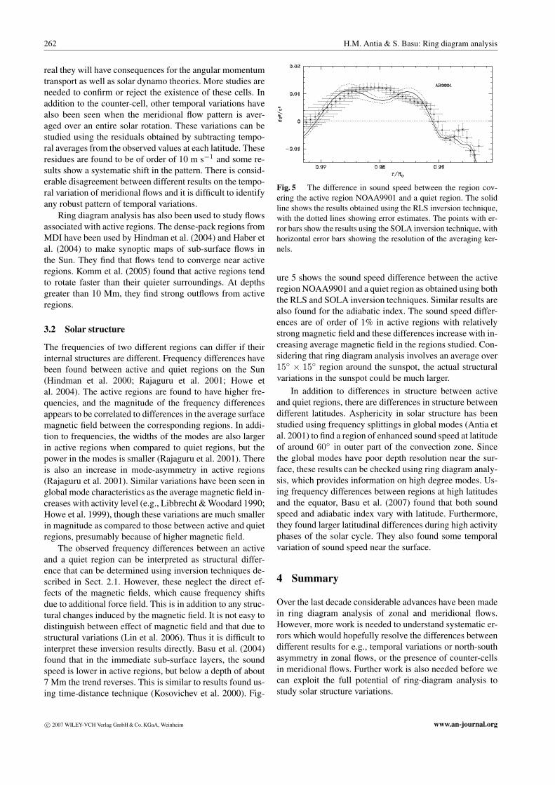
Fig. 5 The difference in sound speed between the region cov-

ering the active region NOAA9901 and a quiet region. The solid

line shows the results obtained using the RLS inversion technique,

with the dotted lines showing error estimates. The points with er-

ror bars show the results using the SOLA inversion technique, with

horizontal error bars showing the resolution of the averaging ker-

nels.

ure 5 shows the sound speed difference between the active

region NOAA9901 and a quiet region as obtained using both

the RLS and SOLA inversion techniques. Similar results are

also found for the adiabatic index. The sound speed differ-

ences are of order of 1% in active regions with relatively

strong magnetic field and these differences increase with in-

creasing average magnetic field in the regions studied. Con-

sidering that ring diagram analysis involves an average over

15◦ × 15◦ region around the sunspot, the actual structural

variations in the sunspot could be much larger.

In addition to differences in structure between active

and quiet regions, there are differences in structure between

different latitudes. Asphericity in solar structure has been

studied using frequency splittings in global modes (Antia et

al. 2001) to find a region of enhanced sound speed at latitude

of around 60◦ in outer part of the convection zone. Since

the global modes have poor depth resolution near the sur-

face, these results can be checked using ring diagram analy-

sis, which provides information on high degree modes. Us-

ing frequency differences between regions at high latitudes

and the equator, Basu et al. (2007) found that both sound

speed and adiabatic index vary with latitude. Furthermore,

they found larger latitudinal differences during high activity

phases of the solar cycle. They also found some temporal

variation of sound speed near the surface.

4 Summary

Over the last decade considerable advances have been made

in ring diagram analysis of zonal and meridional flows.

However, more work is needed to understand systematic er-

rors which would hopefully resolve the differences between

different results for e.g., temporal variations or north-south

asymmetry in zonal flows, or the presence of counter-cells

in meridional flows. Further work is also needed before we

can exploit the full potential of ring-diagram analysis to

study solar structure variations.



Acknowledgements. SB is partially supported by NASA grant

NNG06GD13G, and NSF grant ATM 0348837.

References

Anderson, E.R., Duvall, T.L., Jr., Jefferies, S.M.: 1990, ApJ 364,

699

Antia, H.M., Basu, S.: 1994, A&AS 107, 421

Antia, H.M., Basu, S., Hill, F., Howe, R., Komm, R.W., Schou, J.:

2001, MNRAS 327, 1029

Backus, G.E., Gilbert, J.F.: 1968, Geophys. J. Roy. Astr. Soc. 16,

169

Basu, S., Antia, H.M.: 1999, ApJ 525, 517

Basu, S., Antia, H.M.: 2000a, ApJ 541, 442

Basu, S., Antia, H.M.: 2000b, SoPh 192, 469

Basu, S., Antia, H.M.: 2003, ApJ 585, 553

Basu, S., Antia, H.M., Tripathy, S.C.: 1999, ApJ 512, 458

Basu, S., Antia, H.M., Bogart, R.S.: 2004, ApJ 610, 1157

Basu, S., Antia, H.M., Bogart, R.S.: 2007, ApJ 654, 1146

Bogart, R.S., Basu, S.: 2004, in: D. Danesy (ed), Helio- and Aster-oseismology: Towards a Golden Future, ESA SP-559, p. 329

Dikpati, M., Charbonneau, P.: 1999, ApJ 518, 508

Durney, B.R.: 1993, ApJ 407, 367

Duvall, T.L., Jr., Jefferies, S.M., Harvey, J.W., Pomerantz, M.A.:

1993, Nature 362, 430

Dziembowski, W.A., Pamyatnykh, A.A., Sienkiewicz, R.: 1990,

MNRAS 244, 542

Giles, P.M, Duvall, T.L., Jr., Scherrer, P.H., Bogart, R.S.: 1997,

Nature 390, 52

Gizon, L., Birch, A. C.: 2005, LRSP 2, 6

Gonzalez Hernandez, I., Patron, J.: 2000, SoPh 191, 37

Gonzalez Hernandez, I., et al.: 1999, ApJ 510, L153

Gonzalez Hernandez, I., Komm, R., Hill, F., Howe, R., Corbard,

T., Haber, D.A.: 2006, ApJ 638, 576

Gough, D.O., Thompson, M.J.: 1991, in: A.N. Cox, W.C. Liv-

ingston, M. Matthews (eds.), Solar Interior and Atmosphere,

p. 519

Gough, D.O., et al.: 1996, Sci 272, 1296

Haber, D.A., Hindman, B.W., Toomre, J., Bogart, R.S., Thompson,

M.J., Hill, F.: 2000, Solar Phys. 192, 335

Haber, D.A., Hindman, B.W., Toomre, J., Bogart, R.S., Larsen, R.

M., Hill, F.: 2002, ApJ 570, 855

Haber, D.A., Hindman, B.W., Toomre, J., Thompson, M.J.: 2004,

Solar Physics, 220, 371

Hathaway, D.H., et al.: 1996, Sci 272, 1306

Hill, F.: 1988, ApJ 333, 996

Hill, F.: 1989, ApJ 343, L69

Hill, F.: 1990, SoPh 128, 321

Hindman, B., Haber, D., Toomre, J., Bogart, R.: 2000, SoPh 192,

363

Hindman, B.W., Gizon, L., Duvall, T.L., Haber, D.A., Toomre, J.:

2004, ApJ 613, 1253

Howard, R., LaBonte, B.J.: 1980, ApJ 239, L33

Howe, R., Komm, R., Hill, F.: 1999, ApJ 524, 1084

Howe, R., Christensen-Dalsgaard, J., Hill, F., Komm, R.W.,

Larsen, R.M., Schou, J., Thompson, M.J., Toomre, J.: 2000,

ApJ 533, L163

Howe, R., Komm, R.W., Hill, F., Haber, D.A., Hindman, B.W.:

2004, ApJ 608, 562

Komm, R., Corbard, T., Durney, B.R., Gonzalez Hernandez, I.,

Hill, F., Howe, R., Toner, C.: 2004, ApJ 605, 554

Komm, R., Howe, R., Hill, F., Gonzalez Hernandez, I., Toner, C.,

Corbard, T.: 2005, ApJ 631, 636

Kosovichev, A.G., Duvall, T.L., Jr., Scherrer, P.H.: 2000, SoPh

192, 159

Libbrecht, K.G., Woodard, M.F.: 1990, Nature 345, 779

Lin, C.-H., Li, L.-H., Basu, S.: 2006, in: K. Fletcher (ed.),

SOHO18/GONG 2006/ HELAS I, ESA SP-624, p. 58.1

Nandy, D., Choudhuri, A.R.: 2002, Sci 296, 1671

Nigam, R., Kosovichev, A.G.: 1998, ApJ 505, L51

Patron, J., et al.: 1997, ApJ 485, 869

Pijpers, F.P., Thompson, M.J.: 1992, A&A 262, L33

Pijpers, F.P., Thompson, M.J.: 1994, A&A 281, 231

Rajaguru, S.P., Basu, S., Antia, H.M.: 2001, ApJ 563, 410

Schou, J., Bogart, R.S.: 1998, ApJ 504, L131

Schou, J., et al.: 1998, ApJ 505, 390

Thompson, M.J., et al.: 1996, Sci 272, 1300

Zaatri, A., Komm, R., Gonzalez Hernandez, I., Howe, R., Corbard,

T.: 2006, SoPh 236, 227


Documents

Local helioseismology using ring diagram analysis