The

GovernmeMinistry oStatistics WBanglades

The Bangladesh Bureau of Statistics

in collaboration with

United Nations World Food Programme

Local Estimation of Poverty and Malnutrition in Bangladesh

BANGLADESH 2004

nt of the People’s Republic of Bangladesh f Planning, Planning Division

ing h Bureau of Statistics

ost in need.

Salehuddin M. Musa ndc

Foreword

It is our pleasure to present you a copy of the publication “local estimation of poverty and malnutrition in Bangladesh”. It is the product of close collaboration between the Bangladesh Bureau of Statistics and the World Food Programme, with technical support provided by the Statistics Research and Consulting Centre, Massey University, New Zealand. Future effort by the Government of Bangladesh and its development partners to reduce poverty and malnutrition and to eliminate extreme poverty and hunger, will be guided by the Poverty Reduction Strategy Paper (PRSP) currently being prepared. To reach the targets set for the Millennium Development Goals and those in the PRSP it will be necessary to target resources toward the most deprived and vulnerable areas. Although, general knowledge on the spatial pattern of poverty existed in the country, detailed level information on poverty and malnutrition was lacking. Poverty and nutrition data are generally available up to the Division level through Household Income and Expenditure Surveys, nutrition surveys or surveillance systems. By combining the data from these surveys with the recently conducted census of population, the Bangladesh Bureau of Statistics succeeded in deriving estimates of poverty and malnutrition at the sub-district level. Through the use of Geographic Information Systems technology, the local level estimates have been plotted on a series of user-friendly maps, which will make it very easy to identify areas with high concentrations of poverty and malnutrition. We therefore believe that these maps will be of considerable benefit when a mechanism for aid allocation is required. The study would not have been possible without the hard work, commitment and inputs provided by various institutions and individuals. In particular we would like to thank the following partners for providing technical guidance, data, comments and suggestions: The Bangladesh Bureau of Statistics, the World Food Programmes in Bangladesh, the Statistics Research and Consulting Centre of Massey University, the World Bank, University of California, Berkeley, and the WFP Regional Bureau in Bangkok. Through our collective effort we have contributed to a better understanding of poverty and malnutrition in Bangladesh. Insight into local factors that contribute to people’s poverty and malnutrition status is essential in developing appropriate ways in reaching the PRSP and MDG goals of eliminating extreme poverty and hunger. By knowing where the poor and malnourished are, we should be able to target development resources more effectively and efficiently by ensuring that they are directed to those m Douglad C. Coutts Representative Joint Secretary World Food Programme Bangladesh Statistics Wing, Planning Division

Government of the People’s Republic of Bangladesh

i

Acknowledgement I am happy to know that the report of “local Estimation of Poverty and Malnutrition in Bangladesh” is ready for publication. It is a collaborative effort of Bangladesh Bureau of Statistics and World Food Programme, Dhaka. The findings of this report will help determine the level of poverty incidence and malnutrition at Upazila/thana level. Definitely, this report will be useful in execution of food security programme upto sub- district level. I gratefully recognize the hard work of Professor Stephen Haslett and Dr. Geoffery Jones of the Statistics Research and Consulting Centre, Massey University, New Zealand for using Bangladesh Population Census 2001 data (5% sample), Household Income and Expenditure Survey (HIES) 2000 data and Child Nutrition Survey (CNS) 2000 data in preparing this draft report. I also thank and recognize the sincere work of Mr.Abdul Rashid Sikder, Deputy Director General, Bangladesh Bureau of Statistics for his guiding role in co-ordinating the analytical work. I earnestly acknowledge the contribution of Mr. Faizuddin Ahmed, Director, Mr.Abdul Mallik, Director, Mr. Nowsherwa, Joint Director, Mr. Nowsher Alam, Project Director , Mr. Mainuddin Ahmed, Project Director, Mr. Abdus Salam, Project Director, Mrs. Tajkera Begum, Deputy Director, Mr. Shamsul Alam, Deputy Director, Mr. Zulfiquer Ahmed, Statistical Officer and Mr. Abdus Satter, Statistical Officer of Bangladesh Bureau of Statistics and Mr. Siemon Hollema, Chief Policy & Resourcing Section, Mrs Nusha Yamina Choudhury, Head VAM Unit, and Farah Aziz of World Food Programme (WFP) of Dhaka Office. I also thank Mr. Peter Lanjouw of the World Bank and Mr. Tomoki Fujii of the University of California, Berkeley for their valuable advice. In conclusion, I concede with gratitude the technical and financial support that World Food Programme (WFP), Dhaka had rendered which made it possible to carry out this study. I hope, WFP will continue its collaborative effort for further in depth analysis in future. Suggestions and comments on this report are most welcome. (A.K.M.Musa) Director General Bangladesh Bureau of Statistics

ii

Contents Forward ............................................................................................................................... i Acknowledgement ............................................................................................................. ii Executive Summary .......................................................................................................... iv 1. Introduction .................................................................................................................... 1 2. Methodology .................................................................................................................. 4 3. Data Sources .................................................................................................................. 9 4. Implementation ............................................................................................................ 13 5. Results for Poverty Measures ...................................................................................... 18 6. Results for Malnutrition Measures ............................................................................... 21 7. Conclusions and Discussion ........................................................................................ 23 References ........................................................................................................................ 26 Appendices

A. Auxiliary variables .......................................................................................... 28 B. Regression results ............................................................................................ 30 C. Summary of small-area estimates ................................................................... 33 D. Poverty and nutrition maps ............................................................................. 35

iii

Local Estimation of Poverty and Malnutrition in Bangladesh

Executive Summary

Bangladesh is one of the poorest countries in the world: roughly half of its 126 million citizens live in deprivation, while roughly half of all children under six years show evidence of chronic malnutrition. Poverty and malnutrition in Bangladesh are characterized by regional variation. Factors such as tendency to natural disasters, distribution and quality of land, access to education and health facilities, level of infrastructure development, employment opportunities, and dietary and hygiene practices provide possible explanations for this. Future efforts by the Government and aid agencies to further reduce poverty and malnutrition will be guided by the Interim Poverty Reduction Strategy Paper (I-PRSP) and the full PRSP, currently being prepared, which advocate the use of targeted development programmes directed towards the most deprived and vulnerable areas. This approach should improve the cost-effectiveness of social interventions, but its implementation requires detailed information on poverty and malnutrition at the local level. Indicators for poverty and malnutrition were therefore estimated by applying a variant of the small area estimation technique as pioneered by the World Bank. A five percent sample of the 2001 population census was used in combination with the 2000 Household Income and Expenditure Survey to derive estimates of the poverty incidence, gap and severity at the sub-district level. Estimates were also calculated for average caloric intake and food poverty. Malnutrition estimates are based on the 2000 Child Nutrition Survey. The maps based on these local level estimates are presented in Appendix D. For the poverty estimates a reasonable level of accuracy was achieved, with on the whole acceptable small standard errors, to justify comparison between sub-districts. The poorest areas are found in the Northwest, and the districts of Mymensingh, Netrakona, Bhola and Bandarban (Map D.1). A union level map of poverty was also prepared. As this map is at a finer level -union rather than sub-district- it incorporates information on the accuracy of the poverty estimates by showing the probability that the union has a high incidence (higher than 30 percent) of extreme poverty (Map D.2). A resource allocation map was derived by multiplying the average poverty gap with the total sub-district population. It shows the total monthly resources required to eliminate extreme poverty in all sub-districts. It assumes that there are no additional costs involved in transferring these resources to the extreme poor. Although this assumption is of course unrealistic, the map does provide an indication of the likely cost involved in achieving the MDG / PRSP target of eliminating extreme poverty (Map D.3).

iv

Small area estimates are also calculated for average caloric intake and food poverty, however these are comparatively less accurate, and in general are not precise enough for reliable comparisons to be made between sub-districts (Map D.4 and D.5). Two measures of malnutrition of children under five years age were calculated, namely stunting (low height-for-age) and underweight (low weight-for-age). Due to limitation in local level data on health and caring practices, good predictive models for malnutrition could not be found. The standard errors are 6 percent on average which is perhaps a little too high for reliable comparison to be made between sub-districts and the maps should therefore be regarded as tentative. To account for this, the standard error values were incorporated by calculating the probability that the prevalence of stunting and underweight exceeds 50 percent in a sub-district. According to these maps, malnutrition is particular severe in the coastal belt as well as in the Northern districts of Mymensingh, Netrakona and Sunamganj (Map D.7 and D.9). The poverty and malnutrition maps provide a graphical summary of which areas are suffering from a relatively high deprivation. The main purpose in producing such maps is to aid the planning of social intervention programmes. They could in addition prove useful as a research tool, for example by overlaying geographic, social or economic indicators.

v

Local Estimation of Poverty and Malnutrition in Bangladesh

1. Introduction

1.1 Background Bangladesh is the eighth most populous country in the world, and one of the poorest. Though significant progress has been made in recent years in reducing the incidence of poverty and malnutrition, the fact remains that roughly half of its 126 million citizens live in deprivation, while roughly half of all children under 6 years show some evidence of chronic malnutrition (World Bank, 2003). Poverty and malnutrition in Bangladesh are characterized by regional variation. Factors such as proneness to natural disasters, distribution and quality of land, access to education and health facilities, level of infrastructure development, employment opportunities, and dietary and hygiene practices provide possible explanations for this. Future efforts by the Government and aid agencies to further reduce poverty and malnutrition will be guided by the Interim Poverty Reduction Strategy Paper (I-PRSP) and the full PRSP, currently being prepared, which advocate the use of targeted development programmes directed towards the most deprived and vulnerable areas. This approach should improve the cost-effectiveness of social interventions, but its implementation requires detailed knowledge at local level of incidence and severity. 1.2 Geographic and administrative units Bangladesh is divided into six divisions: Barisal, Chittagong, Dhaka, Khulna, Rajshahi and Sylhet. However, the Household Income and Expenditure Survey, 2000 includes Sylhet in the Chittagong Division, so here is treated as such. Table 1.1 shows the hierarchy of geographic and administrative units in Bangladesh, and their approximate size in terms of number of households. The terms Upazila, Union and Mauza apply in general to rural areas, Thana, Ward and Mahalla to urban or metropolitan.

Table 1.1 The number and size of administrative units at different levels.

division district upazila/thana

union/ ward

mauza/ mahalla

Census contains 5 64 507 5637 59990 Mean no. households 5072464 396286 50024 4499 423

Some knowledge exists on the general spatial pattern of poverty and malnutrition. Recent surveys conducted by the Bangladesh Bureau of Statistics (BBS) give estimates of economic and nutritional status for the whole country and at the division level. However

1

the accuracy of such estimates at a particular level depends crucially on the effective sample size at that level, so that at the district level and below the standard errors of survey-based estimates become too large because each is based on a small number of observations. Effective targeting of aid, as advocated by I-PRSP, requires a nation-wide overview of poverty and nutrition at the upazila, or preferably union, level. Estimates need to be precise, ie with small standard errors, so that the areas with the greatest need are identified correctly. 1.3 Poverty maps The statistical technique of small-area estimation (Ghosh and Rao, 1994, Rao, 1999; Rao, 2003) provides a way of improving survey estimates at small levels of aggregation, by combining the survey data with information derived from other sources, typically a population census. A variant of this methodology has been developed by a research team at the World Bank specifically for the small-area estimation of poverty measures (Elbers, Lanjouw and Lanjouw, 2001). The ELL method has been implemented in several countries including Thailand (Healy, 2003), Cambodia (Fujii, 2002), South Africa (Alderman et al., 2001) and Brazil (Elbers et al. 2001). The methodology is described in detail in the next section. Outputs, in the form of estimates at local level together with their standard errors, can be combined with GIS data to produce a “poverty map” for the whole country, giving a graphical summary of which areas are suffering relatively high deprivation. Our main purpose in producing such maps is to aid the planning of social intervention programmes. They could in addition prove useful as a research tool, for example by overlaying geographic, social or economic indicators. 1.4 Measures of poverty and malnutrition Poverty can be defined in a number of ways. The direct calorie intake (DCI) method is based on per capita calorific intake: the members of a household are considered poor if their average calorie intake falls below a certain level. In Bangladesh “absolute poverty” is defined as an average intake of less than 2122 kcal per capita per day, whilst “hard-core poverty” refers to an average below 1805 kcal per capita per day. In this report, we use a variant of the ELL method to produce a poverty map based on household per capita calorie intake, in addition to the cost-of-basic-needs (CBN) approach used in other implementations of poverty mapping methodology. In the CBN approach poverty lines are calculated to represent the level of per capita expenditure required to meet the basic needs of the members of a household, including an allowance for non-food consumption. First a food poverty line is established, being the amount necessary to meet basic food requirements. Then a non-food allowance is added. The “lower poverty line” adds an amount equal to the typical non-food expenditure of households whose total expenditure

2

is equal to the food poverty line. The “upper poverty line” adds an amount equal to the typical non-food expenditure of households whose food expenditure is equal to the food poverty line. Because prices vary among geographical areas, poverty lines are calculated separately for different regions. Thus in the CBN approach poverty measures are functions of household per capita expenditure. Poverty incidence for a given area is defined as the proportion of individuals living in that area who are in households with an average per capita expenditure below the (lower or upper) poverty line. Poverty gap is the average distance below the poverty line, being zero for those individuals above the line. It thus represents the resources needed to bring all poor individuals up to a basic level. Poverty severity measures the average squared distance below the line, thereby giving more weight to the very poor. These three measures can be placed in a common mathematical framework, the so-called FGT measures (Foster, Greer and Thorbeck, 1984):

)(11

zEIzEz

NP i

N

i

i <⋅

−

= ∑=

α

α (1.1)

where N is the population size of the area, Ei is the expenditure of the ith individual, z is the poverty line and I(Ei < z) is an indicator function (equal to 1 when expenditure is below the poverty line, and 0 otherwise). Poverty incidence, gap and severity correspond to α = 0, 1 and 2 respectively. In this report we estimate all six values (three measures for each of two poverty lines) at the upazila level. In practice we find that all six are highly correlated, so that a single poverty map showing lower poverty incidence captures most of the available information on the geographical distribution of poverty. Two measures of malnutrition are considered, based on measurements of a child’s height and weight. Stunting or low height-for-age is defined as having a height at least two standard deviations below the median height for a reference population. Underweight or low weight-for-age is similarly defined. The data used as a reference standard in these definitions was established in 1975 by the National Center for Health Statistics/Centers for Disease Control in the USA (Hamill, Dridz, Johnson, Reed et al., 1979). In this report we consider the nutrition status of children between the ages of 6 and 66 months. Within a particular region stunting is defined as the proportion of such children with a standardized height-for-age (HAZ) value below –2. Similarly underweight is the proportion with a standardized weight-for-age (WAZ) value below –2. Stunting can be regarded as evidence of chronic malnutrition. Underweight on the other hand reflects both chronic malnutrition and acute malnutrition. It is a current condition resulting from inadequate food intake, past episodes of undernutrition or poor health conditions. Our aim in this report is to construct upazila-level maps for both measures.

3

2. Methodology We present in this section a brief overview of small-area estimation and the ELL method. Details of the implementation in Bangladesh are given in Section 4. 2.1 Small area estimation Small area estimation refers to a collection of statistical techniques designed for improving sample survey estimates through the use of auxiliary information (Ghosh and Rao, 1994; Rao, 1999; Rao, 2003). We begin with a target variable, denoted Y, for which we require estimates over a range of small subpopulations, usually corresponding to small geographical areas. (In this report Y is either per capita expenditure or its derived measures, per capita calorie intake, standardized height-for-age or standardized weight-for-age.) Direct estimates of Y for each subpopulation are available from sample survey data, in which Y is measured directly on the sampled units (households or eligible children). Because the sample sizes within the subpopulations will typically be very small, these direct estimates will have large standard errors so will not be reliable. Indeed, some subpopulations may not be sampled at all in the survey. Auxiliary information, denoted X, can be used under some circumstances to improve the estimates, giving lower standard errors. In the situations examined in this report, X represents additional variables that have been measured for the whole population, either by a census or via a GIS database. A relationship between Y and X of the form

uXY += β

can be estimated using the survey data, for which both the target variable and the auxiliary variables are available. Here β represents the estimated regression coefficients giving the effect of the X variables on Y, and u is a random error term representing that part of Y that cannot be explained using the auxiliary information. If we assume that this relationship holds in the population as a whole, we can use it to predict Y for those units for which we have measured X but not Y. Small-area estimates based on these predicted Y values will often have smaller standard errors than the direct estimates, even allowing for the uncertainty in the predicted values, because they are based on much larger samples. Thus the idea is to “borrow strength” from the much more detailed coverage of the census data to supplement the direct measurements of the survey. 2.2 Clustering The units on which measurements have been made are often not independent, but are grouped naturally into clusters of similar units. Households tend to cluster together into villages or other small geographic or administrative units, which are themselves relatively homogenous. Put simply, households that are close together tend to be more similar than

4

households far apart. When such structure exists in the population, the regression model above can be more explicitly written as

ijiijij ehXY ++= β (2.1)

where Yij represents the measurement on the jth unit in the ith cluster, hi the error term held in common by the ith cluster, and eij the household-level error within the cluster. The relative importance of the two sources of error can be measured by their respective variances and . Ghosh and Rao (1994) give an overview of how to obtain small-area estimates, together with standard errors, for this model.

2hσ 2

eσ

We note that the auxiliary variables Xij may be useful primarily in explaining the household-level variation, or the cluster-level variation. The more variation is explained at a particular level, the smaller the respective error variance, or . The estimate for a particular small area will typically be the average of the predicted Ys in that area. Because the standard error of a mean gets smaller as the sample size gets bigger, the contribution to the overall standard error of the variation at each level, household and cluster, depends on the sample size at that level. The number of households in a small area will typically be much larger than the number of clusters, so to get small standard errors it is of particular importance that the unexplained cluster-level variance should be small. Two important diagnostics of the model-fitting stage, in which the relationship between Y and X is estimated for the survey data, are the R

2hσ

2e

2eσ

2hσ

2 measuring how much of the variability in Y is explained by X, and the ratio / ( + ) measuring how much of the unexplained variation is at the cluster level. Note that although and are parameters they are different for different models with different regressors. GIS data and cluster-level means should be particularly useful in lowering this ratio.

2hσ 2

hσ σ2hσ 2

eσ

Another important aspect of clustering is its effect on the estimation of the model. The survey data used for this estimation cannot be regarded as a random sample, because they have been obtained from a complex survey design involving stratification and cluster sampling. To account properly for the survey design requires the use of specialized statistical routines (Skinner et al., 1989; Chambers and Skinner, 2003) in order to get consistent estimates for the regression coefficient vector β and its variance Vβ . 2.3 The ELL method The ELL methodology was designed specifically for the small-area estimation of poverty measures based on per capita household expenditure. Here the target variable Y is log-transformed expenditure, the logarithm being used to make more symmetrical the highly right-skewed distribution of untransformed expenditure. It is assumed that measurements on Y are available from a survey. The first step is to identify a set of auxiliary variables X that are in the survey and are also available for the whole population. It is important that these should be defined and

5

measured in a consistent way in both data sources. The model (2.1) is then estimated for the survey data, using ordinary least squares but incorporating aspects of the survey design for example through use of the “expansion factors” or inverse sampling probabilities. The residuals u from this analysis are used to define cluster-level residuals

, the dot denoting averaging over j, and household-level residuals e . ijˆ

⋅= ii uh ˆˆijiij uh ˆˆˆ −=

It is assumed that the cluster-level effects hi all come from the same distribution, but that the household-level effects eij may be heteroscedastic. This is modelled by allowing the variance to depend on a subset Z of the auxiliary variables: 2

eσ

rZg e += ασ )( 2

where g(.) is an appropriately chosen link function, α represents the effect of Z on the variance and r is a random error term. Fujii (2003) uses a version of the more general model of Elbers et al. (2002) involving a logistic-type link function, fitted using the squared household-level residuals. Fujii’s model is:

ijijij

ij rZeA

e+=

−α2

2

ˆˆ

ln (2.2)

From this model the fitted variances can be calculated and used to produce

standardized household-level residuals . These can then be mean-corrected to sum to zero, either across the whole survey data set or separately within each cluster.

2,ˆ ijeσ

ij e* ˆˆ = ijeije ,ˆ/σ

In standard applications of small-area estimation, the estimated model (2.1) is applied to the known X values in the population to produce predicted Y values, which are then average over each small area to produce a point estimate, the standard error of which is inferred from appropriate asymptotic theory. In the case of poverty mapping, our interest is not always directly in Y but in several non-linear functions of Y (see section 1.4). The ELL method obtains unbiased estimates and standard errors for these by using a bootstrap procedure, so that there are many α ’s and hence many generated by simulation and

this is what allows estimation of (via its bootstrap analogue) for given i and j. ije

2,ijeσ

2.4 Bootstrapping Bootstrapping is the name given to a set of statistical procedures that use computer-generated random numbers to simulate the distribution of an estimator (Efron and Tibshirani, 1993). In the case of poverty mapping, we construct not just one predicted value

βˆijij XY =

6

(where represents the estimated coefficients from fitting the model) but a large number of alternative predicted values

β

bij

bi

bij

bij ehXY ++= β , b BK,1=

in such a way as to take account of the variability of the predicted values. We know that is an unbiased estimator of β with variance Vβ β , so we draw each βb independently

from a multivariate normal distribution with mean and variance matrix Vβ β . The cluster-level effects are taken from the empirical distribution of hb

ih i, ie drawn randomly

with replacement from the set of cluster-level residuals . To take account of unequal variances (heteroscedasticity) in the household-level residuals, we first draw α

ihb from a

multivariate normal distribution with mean α and variance matrix Vα, combine it with Zij to give a predicted variance and use this to adjust the household-level effect

bije

bij

bij ee ,

* σ×=

where represents a random draw from the empirical distribution of e , either for the whole data set or just within the cluster chosen for h

bije* *

ij

i (consistently with the mean-centring of section 2.3). Each complete set of bootstrap values Y , for a fixed value of b, will yield a set of small-area estimates. In the case of poverty estimates we exponentiate each Y to give predicted expenditure E

bij

ij = exp(Yij), then apply equation (1.1). The mean and standard deviation of a particular small-area estimate, across all b values, then yields a point estimate and its standard error for that area. 2.5 Interpretation of standard errors The standard error of a particular small-area estimate is intended to reflect the uncertainty in that estimate. A rough rule of thumb is to take two standard errors on each side of the point estimate as representing the range of values within which we expect the true value to lie. When two or more small-area estimates are being compared, for example when deciding on priority areas for receiving aid, the standard errors provide a guide for how accurate each individual estimate is and whether the observed differences in the estimates are indicative of real differences between the areas. They serve as a reminder to users of poverty maps that the information in them represents estimates, which may not always be very precise. A way of incorporating the standard errors into a poverty map is suggested in section 4. The size of the standard error depends on a number of factors. The poorer the fit of the model (2.1), in terms of small R2, large or , the more variation in the target variable will be unexplained and the greater will be the standard errors of the small-area estimates. The population size, in terms of both the number of households and the

2hσ 2

eσ

7

number of clusters in the area, is also an important factor. Generally speaking, standard errors decrease proportionally as the square root of the population size. Standard errors will be acceptably small at higher geographic levels but not at lower levels. If we decide to create a poverty map at a level for which the standard errors are generally acceptable, there will be some, smaller, areas for which the standard errors are larger than we would like. The sample size used in fitting the model is also important. The bootstrapping methodology incorporates the variability in the estimated regression coefficients α , . If the sample size is small these estimates will be very uncertain and the standard errors of the small-area estimates will be large. This problem is also affected by the number of explanatory variables included in the auxiliary information, X and Z. A large number of explanatory variables relative to the sample size increases the uncertainty in the regression coefficients. We can always increase the apparent explanatory power of the model (ie increase the R

β

2 from the survey data) by increasing the number of X variables, or by dividing the population into distinct subpopulations and fitting separate models in each, but the increased uncertainty in the estimated coefficients may result in an overall loss of precision when the model is used to predict values for the census data. We must take care not to “over-fit” the model. There will be some uncertainty in the estimates, and indeed the standard errors, due to the bootstrapping methodology, which uses a finite sample of bootstrap estimates to approximate the distribution of the estimator. This could be decreased, at the expense of computing time, by increasing the number of bootstrap simulations B. Finally, the integrity of the estimates and standard errors depends on the fitted model being correct, in that it applies to the population in the same way that it applied to the sample. This relies on good matching of survey and census to provide valid auxiliary information. We must also take care to avoid, as much as possible, spurious relationships or artefacts which appear, statistically, to be true in the sample but do not hold in the population. This can be caused by fitting too many variables, but also by choosing variables indiscriminately from a very large set of possibilities. Such a situation could lead to estimates with apparently small standard errors, but the standard errors would be spurious. For this reason the final step in poverty mapping, field verification, is extremely important.

8

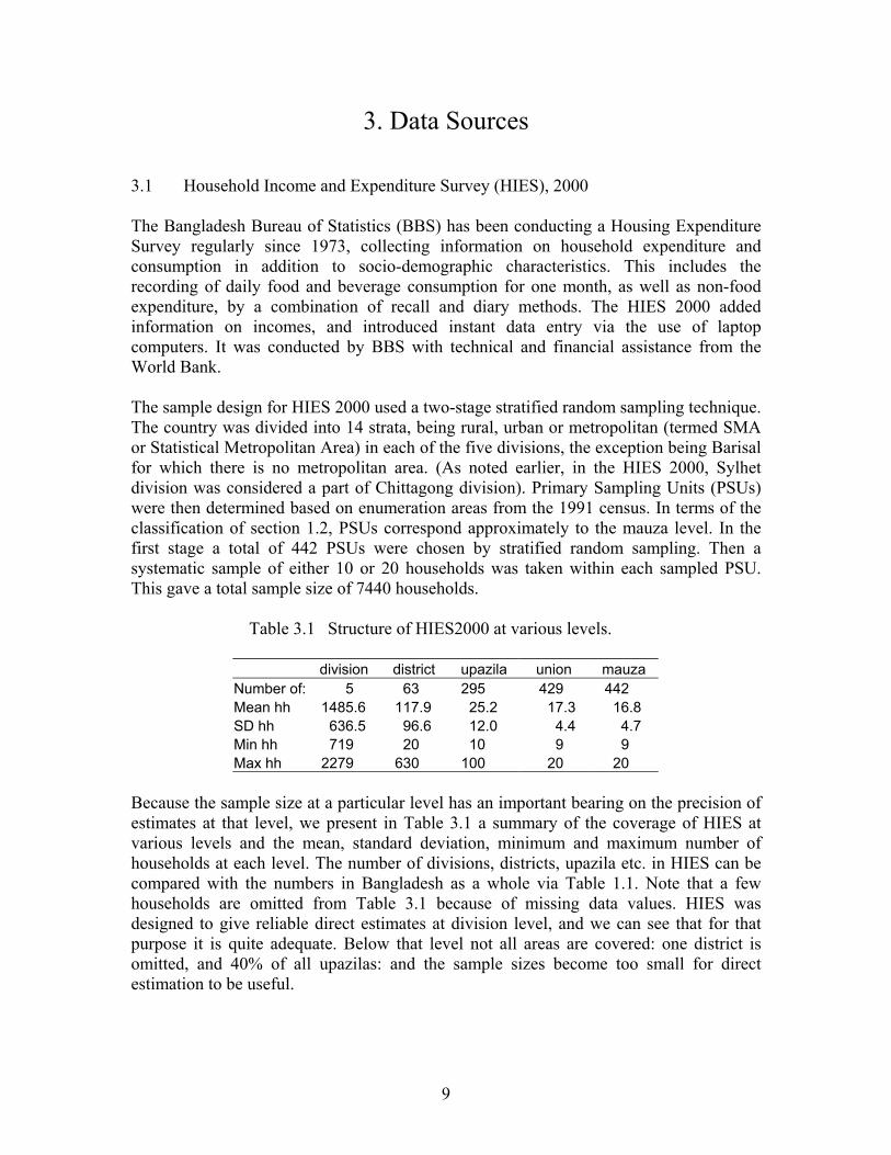
3. Data Sources 3.1 Household Income and Expenditure Survey (HIES), 2000 The Bangladesh Bureau of Statistics (BBS) has been conducting a Housing Expenditure Survey regularly since 1973, collecting information on household expenditure and consumption in addition to socio-demographic characteristics. This includes the recording of daily food and beverage consumption for one month, as well as non-food expenditure, by a combination of recall and diary methods. The HIES 2000 added information on incomes, and introduced instant data entry via the use of laptop computers. It was conducted by BBS with technical and financial assistance from the World Bank. The sample design for HIES 2000 used a two-stage stratified random sampling technique. The country was divided into 14 strata, being rural, urban or metropolitan (termed SMA or Statistical Metropolitan Area) in each of the five divisions, the exception being Barisal for which there is no metropolitan area. (As noted earlier, in the HIES 2000, Sylhet division was considered a part of Chittagong division). Primary Sampling Units (PSUs) were then determined based on enumeration areas from the 1991 census. In terms of the classification of section 1.2, PSUs correspond approximately to the mauza level. In the first stage a total of 442 PSUs were chosen by stratified random sampling. Then a systematic sample of either 10 or 20 households was taken within each sampled PSU. This gave a total sample size of 7440 households.

Table 3.1 Structure of HIES2000 at various levels.

division district upazila union mauza Number of: 5 63 295 429 442 Mean hh 1485.6 117.9 25.2 17.3 16.8 SD hh 636.5 96.6 12.0 4.4 4.7 Min hh 719 20 10 9 9 Max hh 2279 630 100 20 20

Because the sample size at a particular level has an important bearing on the precision of estimates at that level, we present in Table 3.1 a summary of the coverage of HIES at various levels and the mean, standard deviation, minimum and maximum number of households at each level. The number of divisions, districts, upazila etc. in HIES can be compared with the numbers in Bangladesh as a whole via Table 1.1. Note that a few households are omitted from Table 3.1 because of missing data values. HIES was designed to give reliable direct estimates at division level, and we can see that for that purpose it is quite adequate. Below that level not all areas are covered: one district is omitted, and 40% of all upazilas: and the sample sizes become too small for direct estimation to be useful.

9

The HIES report (BBS, 2003) gives country-wide and division level estimates of poverty as defined in section 1.4, together with their standard errors. It also gives details of the calculation of poverty lines, and analyses of demographic variables and their relationship with poverty incidence. A list of the auxiliary variables available or derivable from the HIES database and matchable to census data is given in Appendix A.1. The target variables available in HIES and used in this study are monthly per capita consumption expenditure and daily per capita calorie intake, averaged at the household level. 3.2 Child Nutrition Survey (CNS), 2000 The Child Nutrition Survey has been carried out regularly by BBS, with financial assistance from UNICEF, since 1985. The survey is designed to give national level data on the nutritional status of children in the country and the factors affecting it. Anthropometrical measures are taken on selected children to determine nutritional status as described in section 1.4, in addition to detailed information on household demographic characteristics, environmental conditions and child feeding and caring practices. Because CNS is conducted on eligible children from households sampled in the HIES survey, all HIES variables can be considered part of the CNS data set. CNS 2000 covered 4000 children aged 6-71 months. For reasons of compatibility with census data, we used only those aged 6-66 months. Most contributing households had only one eligible child, but 25% had two or more (see Table 3.2).

Table 3.2 Structure of CNS2000.

No. of children 1 2 3 4 TotalNo. of households 2194 660 49 11 2914

At upazila level, of the 300 upazilas represented the mean number of children selected was 12.4, the minimum 1 and the maximum 53. It is clear from this that direct estimates of stunting and underweight at this level would not be reliable. The CNS 2000 report (BBS, 2002) gave the national prevalence of stunting as 48.8%, and underweight 51.1%. These represent small but statistically significant decreases from the previous survey in 1995. Statistically significant relationships were found between nutritional status and a number of variables classified broadly into household food security factors, health parameters and child caring practices. Despite the wealth of detailed information available in CNS, the only additional information on each child, apart from the HIES variables, that could be matched with the more economically focused census data for our analysis were age and sex. 3.3 Census, 2001 The fourth decennial population census of Bangladesh was conducted by BBS on 23-27 January 2001, the official census night being 22-23 January. The census questionnaire

10

consisted of two modules, with the first 16 questions being related to housing and general household characteristics and the remaining 12 questions related to individuals within the household. Information was obtained through interviewing the head of household or other responsible household member. Data were entered on special forms designed for reading by Optical Character Reader (OCR) and Optical Mark Reader (OMR). Those individuals not at home on census night are considered to be “floating” and were counted in the place where they were staying that night. Households were classified as dwelling, institutional (eg hostels, hospitals, jails) or other (eg people living in offices). Since the HIES data only covered residential households, it was decided to exclude institutional and other types from the census data set. In conjunction with the enumeration of the population, a mapping operation was undertaken to update regional boundaries. In urban areas old maps of wards and mahallas were updated and new maps prepared where necessary, demarcating new boundaries. Similarly in rural areas union and mauza maps were updated. One important consequence of this updating is the difficulty in matching pre-census data sets, such as HIES2000, with the new census data at union level or below. The population on census night was declared to be 123.8 million. The processing of such a vast amount of data is clearly a mammoth task and it is not yet complete: the checking and editing of the forms prior to OMR/OCR entry is ongoing. In order to provide some preliminary results, BBS took a 5% sample by systematic sampling of enumeration areas within each upazila. This cluster sample has been fully edited, entered and analysed with the results being published as a provisional report (BBS, 2003) pending the availability of the full census data. It is this 5% sample with which we work in this report.

Table 3.3 Structure of 5% Census at various levels.

district upazila union mauzaNumber of: 64 507 5637 12170Mean hh 19660.0 2481.7 223.2 103.4SD hh 13448.6 1337.0 142.2 49.2Min hh 2564 157 1 1Max hh 88585 9568 2102 1132

Table 3.3 shows the coverage of the 5% sample. By comparison with Table 1.1 we can see that all unions are sampled from but not all mauza. In addition there are some unions with very few sampled households presumably because, although complete enumeration areas were sampled, some would have contained institutional or other types that have been eliminated. Even at upazila level there are a few areas with relatively small numbers of available households. This puts a restriction on how finely we can analyse data in small-area estimation at present, until the full census becomes available.

11

Census variables were averaged at upazila level to create a new dataset that could be merged with both the survey and census data. A list of these census mean variables is given in Appendix A.2. 3.4 Geographical Information System (GIS) data A set of geographic indicators at union level was prepared by the Vulnerability Analysis and Mapping (VAM) Unit of WFP, Dhaka. This involved compiling a number of data sets from various sources into a GIS and generating indictors for each union. Cost-distance calculation, for example distance to nearest hospital or growth centre, were performed by using IDRISI Kilimanjaro software (Clark University), by transforming vector data into raster data. The road and river network were taken into account in these calculations. Other GIS operations were undertaken in ArcGIS (ESRI). A list of the indicators generated is given in Appendix A.3. As with HIES, there is a mismatch between the union boundaries and those of the 2001 census. This made it difficult to match the GIS data with the census and HIES data. No updated boundary data is as yet available.

12

4. Implementation 4.1 Selection of auxiliary data The auxiliary data X used to predict the target variable Y can be classified into two types: the survey variables, obtainable or derivable from the survey at household or individual level, and the location variables applying to particular geographic units. The latter include averages of census variables at a particular geographical level, and various Geographical Information System (GIS) variables. As noted earlier, it is important that any auxiliary variables used in modelling and predicting should be comparable in the estimation (survey) data set and the prediction (census) data set. In the case of survey variables, we begin by examining the survey and census questionnaires to find out which questions in each elicit equivalent information. In some cases equivalence may be achieved by collapsing some categories of answers. For example in the census questionnaire there are four categories for Building Type, translated as temporary, tin roof, semi-pucca and pucca. In HIES there was a lot more detailed information on the type of building, but careful discussion produced from this a categorization felt to be equivalent to the census variable. When common variables have been identified the appropriate statistics are compared for the survey and census data. In the case of categorical data we compare proportions in each category: for numerical data, such as household proportion of females, we compare the means and standard deviations. For this purpose confidence intervals can be calculated for the relevant statistics in the survey data set, taking account of the stratification and clustering in the sample design. The equivalent statistic for the census data should be within the confidence interval for the survey. In some cases variables were dropped at this stage. Even an apparently clearly-defined variable like Sex of Head of Household was found to give significantly different proportions between census and survey, possibly because of a differing treatment of households where the male head of household is working overseas. The inclusion of location effect variables should be straightforward since they can be merged with the survey and census data using indicators for the geographical unit to which each household or individual belongs. This can be problematic in practice however, because of changing boundaries and the creation of new unions and wards. The HIES survey, the 2001 census and the GIS data all used different versions so that it was not possible to merge with both survey and census in a comparable way at union level. As an alternative, upazila-level census means were merged successfully with both data sets. The GIS data, even at upazila level, did not completely cover the census data with some, mostly urban, areas being missed. One alternative explored was to fit separate models for those areas where GIS data was available, but it was found that the GIS variables added little extra in terms of explanatory power. This is an area where further general research is needed, as the central technical problem extends beyond this study. Once all usable auxiliary data have been assembled, it may be necessary to delete some cases where there are missing values or outliers. In our case several HIES households had

13

missing location information and two were missing one variable. Two individuals were removed from CNS because of unusually high HAZ values. In the census data there were some households with very large numbers of members, even after deletion of institutional and other types. A similar problem was noted by Fujii (2003) for Cambodia. We decided to delete those households with more members than the maximum in the HIES survey, ie 26. This seemed a reasonable course of action as HIES was known to contain only general residential households. 4.2 First stage regressions The selection of an appropriate model for (2.1) is a difficult problem. We have a large number of possible predictor variables (28 + 25 + 10 = 63: see Appendix A) to choose from, with inevitably a good deal of interrelationship between them in the form of multicollinearity. If we also include two-way interactions there are well over a thousand. (A “two-way interaction” is the product of two basic or “main-effect” variables). Squares or other transformations of numerical variables could also be considered. As noted in section 2.5, we must be careful not to over-fit, so the number of predictors included in the model should be small compared to the number of observations in the survey, but there is also the problem of selecting a few variables from the large number available which appear to be useful, only to find (or even worse, not find) that an apparently strong statistical relationship in the survey data does not hold for the population as a whole. The search for significant relationships over such a large collection of variables must inevitably be automated to a certain extent, but we have chosen not to rely entirely on automatic variable selection methods such as stepwise or best-subsets regression. Firstly the principle of hierarchical modelling has been adopted in general, in which higher-order terms such as two-way interactions are included in the model only if their corresponding main-effects are also included. Thus we begin with main-effects only, and add interaction and nonlinear terms carefully and judiciously. We look not just for statistical significance but also for a plausible relationship. For example, the effect of household size on log expenditure was expected to be nonlinear, with both small and large households tending to have larger per capita expenditure. The square of household size, centred around the mean, was added and found to be significant. Other implementations of ELL methodology have fitted separate models for each stratum defined by the survey design. This has the advantage of tailoring the model to account for the different characteristics of each stratum, but it can increase the problem of over-fitting if some strata are small. We chose initially to try for one model across the whole country. This has the advantage of more stable parameter estimates and a better chance of finding genuine relationships that apply outside of the estimation data. Bangladesh is relatively homogenous at the division level, and the classification of non-rural into urban or metro, used for the HIES stratification, did not appear to match well with the census data. We found that a single model fitted well for log expenditure, with different intercepts for each division and interaction terms to allow the effects of some variables to vary from rural to non-rural (see Appendix B.1).

14

We were less successful for the other target variables (log kilocalories, HAZ and WAZ). Despite our preference for a single model, we were unable to find models with sufficient explanatory power, so decided after discussion with WFP staff to experiment with an alternative stratification based on six relative homogenous zones as presented in Appendix B.3 (Chittagong Hill Tracts, North-East, Coastal, Eastern, Central and Northern). This did give some apparent improvement in R2 values as well as much lower variance ratios, but a few of these ecozones had small numbers of sampled households in the survey data so only simple models could be fitted (see Appendix B.4-6). Whether the apparent improvement in predictive power is genuine or spurious remains to be investigated by field verification. The present models for these variables, and the small-area estimates derived from them, should be regarded as tentative at this stage pending the availability of mergeable GIS data. Regarding transformation of the target variable, we found that calorie intake, like expenditure, was highly right-skewed, so used a log transform for both. We found however that height-for-age and weight-for-age were already approximately symmetrical with no evidence of skewness, so no transformation was applied in modelling these two. We also departed from the usual ELL implementation in our use of a single-stage, robust regression procedure for estimating model (2.1), rather than the two-stage procedure of ordinary least squares followed by estimation of a variance matrix for generalized least squares. This gives the advantages of properly accounting for the survey design and obtaining consistent estimates of the covariance matrices in a single step. These covariance matrices were saved, along with the parameter estimates and both household- and cluster-level residuals (as defined in section 2.3), for implementation of the prediction step. 4.3 Heteroscedasticity modelling Like Healey (2003) we amended the regression model (2.2) for the household-level variance to prevent very small residuals from becoming to influential. We used a slightly different amendment:

ijijij

ijij rZ

eAe

L +=

−

+≡ α

δ2

2

ˆˆ

ln

where δ is a small positive constant and A is chosen to be just larger than the largest e

(eg δ = 0.0001, ). These choices can be justified empirically by graphical examination of the L

2ˆij

2ˆmax05.1 ijeA ×=

ij, which should show neither abrupt truncation nor extreme outliers. The predicted value of the household-specific variance, using the delta method, then becomes:

+

−++

+

−= 3

22, )1(

)1()(ˆ

21

1 ij

ijijr

ij

ijije B

BBAB

AB δσ

δσ

15

where B = eZα. The variance model fitted for log expenditure is shown in detail in Appendix B.2. There was no appreciable heteroscedasticity for log kilocalories. A summary of the results for the other models is given in Appendices B. 5-6. These models for variance essentially control for outliers, by adjusting or shrinking large residuals toward zero. They form an explicit part of the ELL methodology. Other forms are possible, but in keeping with the need to maintain international comparison, for example with Cambodia and South Africa, the ELL model has been used here.

ije

4.4 Simulation of predicted values Simulated values for the model parameters α and β were obtained by parametric bootstrap, ie drawn from their respective sampling distributions as estimated by the survey regressions. Simulation of the cluster-and standardized household-level effects hi and e*

ij presents several possible choices. A parametric bootstrap could be used by fitting suitable distributions (eg Normal, t) to the residuals and drawing randomly from these. We chose here a non-parametric bootstrap in which we sample with replacement from the residuals, ie from the empirical distributions. Other implementations have chosen to truncate these distributions by deleting extreme values from the residuals. We have not done this. Graphical examination of the two sets of residuals showed that the distributions were long-tailed but there was no compelling justification for eliminating the tail values. Another choice is whether to resample the e from the full set or only from those within the cluster corresponding to the chosen h

*ij

i. We chose the latter, so when mean-correcting the standardized residuals (see section 2.3) we used

∑=

−=in

jijeij

iijeijij e

nee

1,,

* ˆ/ˆ1ˆ/ˆˆ σσ

Note that mean correction when needed can bee an indication of the extent of any bias in the bootstrap and hence of an incorrect regression model, so it is encouraging that mean corrections here were small in relative terms. A total of 100 bootstrap predicted values

were produced for each unit in the census and for each target variable, as described in section 2.4.

bijY

4.5 Production of final estimates Since a log transform was applied in modelling expenditure and calorie intake, we first reverse this transformation by exponentiating, eg predicted expenditure . The predicted values can then be grouped at the appropriate geographic level. We used primarily upazila level, but also investigated the accuracy of union-level estimates. Once the predicted values have been produced and stored it is easy to investigate alternative levels of accumulation, using the standard errors as a guide to what is an appropriate level.

bijYb

ij eE =

16

For expenditure and calorie intake the census units are households and the target variables per capita average values, so the accumulation needs to be weighted by household size. Thus for example the formula for the bth bootstrap estimate of poverty incidence (α = 0 in equation 1.1) in region R is amended to:

bRP

∑∑∈∈

<⋅=Rij

ijRij

bijij

bR nzEInP )(

where nij is the size of household ij in R. The census units for height-for-age and weight-for-age are individual children, so no weighting is required. For example the estimated incidence of stunting for region R is:

RRij

bij

bR NHAZIS /)00.2(∑

∈

−<=

where NR is the number of eligible children in R. The 100 bootstrap estimates for each region, eg were summarized by their mean and standard deviation, giving a point estimate and a standard error for each region.

1001RR PP K

17

5. Results for Poverty Measures 5.1 Results for expenditure-based poverty measures The results for the six poverty measures (incidence, gap and severity at lower and upper poverty lines), and average calorie intake, were first accumulated at the division level and compared with the survey estimates from HIES.

Table 5.1 Comparison of division-level estimates of lower poverty incidence

HIES se lcl ucl SAE se Div1 0.2632 0.0326 0.1993 0.3272 0.3023 0.0252 Div2 0.2263 0.0202 0.1866 0.2659 0.2338 0.0109 Div3 0.2802 0.0193 0.2422 0.3181 0.2513 0.0139 Div4 0.2833 0.0248 0.2347 0.3319 0.2684 0.0200 Div5 0.3999 0.0223 0.3563 0.4435 0.3810 0.0149

Table 5.1 shows the comparison for lower poverty incidence. The small-area estimates (SAE in the table) calculated using both census and survey data can be seen to lie within the lower and upper confidence limits (lcl to ucl) calculated just using the survey data but allowing for the sampling design. Thus there can be said to be agreement at division level. The standard errors in each case are seen to be smaller for the small-area estimates: this represents the gain in precision from adding the census information. More detailed results, for all six measures, are presented in Appendix C.1. Here we find that although there is still general agreement, there are a few small-area estimates which lie outside of their respective HIES confidence intervals, in particular the gap and severity measures for Division 1. This is possibly because these measures are sensitive to outliers particularly when sample sizes are small, and we have not truncated the distributions of the residuals.

Table 5.2 Summary of upazila-level small-area estimates of lower poverty incidence

# Obs Mean Std. Dev. Min Max Estimate 507 0.2930 0.1063 0.0014 0.5531 se 507 0.0388 0.0146 0.0025 0.1145

A summary of the small-area estimates and their standard errors at upazila level is given in Table 5.2 for lower poverty incidence, with more detailed results on all six measures in Appendix C.2. For the 507 upazilas in Bangladesh the estimated lower poverty incidence ranges from 0.001 to 0.553. The standard errors vary considerably, from 0.003 to 0.115 with an average of 0.039 (or about 4%). This could be considered to be a reasonable level of accuracy for making comparisons between upazilas. A map based on these estimates is shown in Appendix D.1. Figure 5.1 shows how the standard errors are related to the estimates. As is usual with estimated proportions, they are least accurate when the proportion is close to 0.5. Those

18

estimates with particularly large standard errors relate to upazilas with smaller numbers of households in the 5% census. For exploratory purposes, pending the availability of the full census data, we also examined union-level estimates. Here the standard errors become much larger, with in some cases very few data points. We explored for these estimates a possible way of incorporating the standard errors into a poverty map, first calculating standardized departures from a pre-specified incidence level, say 30%, as

errorstandard30.0estimate −

=Z

and then transforming this into a probability assuming a normal distribution. This value can then be mapped, as in Appendix D.2, and interpreted as the probability that the corresponding union has a poverty incidence at least as high as the pre-chosen level. Thus when targeting aid we could focus on those area which we believe have the greatest chance of exceeding a threshold poverty incidence. This suggestion is novel, and its utility will have to be examined with reference to field data

Figure 5.1 Upazila-level lower poverty incidence estimates and their standard errors

0.0

5.1

.15

Sta

ndar

d er

ror

0 .2 .4 .6Low er poverty incidence

We also calculated the total resources needed by upazila to bring all the extreme poor individuals up to the level of the lower poverty line, assuming that there are no additional cost involved in transferring these resources. This was done by multiplying the poverty gap estimates with the total upazila population. The map is presented in Appendix D.3. 5.2 Results for calorie intake measures Estimates of average calorie intake were first accumulated at the zone level and compared with estimates derived solely from the HIES survey. Results are given in Table 5.3. Because the models fitted to the logarithm of calorie intake, ie to loge(kilocalories), were quite poor in explanatory power (R2 around 20-30%) these results should be regarded as tentative. We see that the small-area estimate for each zone is within the corresponding

19

HIES-based confidence interval, but this is not surprising as separate models were fitted for each zone. It is encouraging however, that the standard errors for the small-area estimates still succeed in being lower than those from the survey only, and this seems likely to reflect the aggregation into small areas of models fitted to individual data, ie the aggregation will balance out the small R2 value for individual level data in the absence of appreciable measurement error or model bias.

Table 5.3 Comparison of zone-level estimates of average kilocalorie intake

HIES se lcl ucl SAE se Zone 1 2590.42 99.49 2391.89 2788.95 2564.06 47.00 Zone 2 2419.00 40.53 2338.11 2499.88 2414.89 16.43 Zone 3 2254.25 27.72 2199.56 2308.94 2283.48 22.00 Zone 4 2308.13 33.54 2241.77 2374.49 2291.49 21.69 Zone 5 2196.55 24.31 2148.73 2244.37 2238.57 22.85 Zone 6 2187.73 28.73 2130.98 2244.48 2203.89 19.38

A summary of the upazila-level estimates is given in Table 5.4. We note that the standard deviation of these estimates, representing the variability in the estimates from upazila to upazila, is about 190 kilocalories, whereas the average standard error of the estimates themselves is about 84 kilocalories. Thus some discrimination between upazilas should be possible using these figures, but in general they are not precise enough for reliable comparisons to be made.

Table 5.4 Summary of upazila-level estimates of average kilocalorie intake

# Obs Mean Std. Dev. Min Max Estimate 507 2284.28 189.78 1683.50 3570.79 Se 507 84.13 30.71 25.96 309.45

We also used the predicted calorie intake data to produce upazila-level estimates of food poverty incidence, using the absolute poverty line based on an intake of 2122 kilo calorie per capita per day and the hard core poverty line of 1805 kilo calorie per capita per day. Again the results are somewhat tentative because of a lack of explanatory power at individual level, although the earlier comments about the compensation due aggregation in the absence of systematic measurement error and/or model bias again apply.

20

6. Results for Malnutrition Measures 6.1 Results for stunting As noted earlier, the first stage regression models for height-for-age were poor in terms of predictive power, the R2 values being mostly 10-20% (see Appendix B.5). Despite this, it appears from Table 6.1 that the small-area estimates of stunting at zone level still have smaller standard errors than the direct estimates from the CNS survey.

Table 6.1 Comparison of zone-level estimates of stunting

CNS se lcl ucl SAE se Zone 1 0.3704 0.1352 0.1055 0.6354 0.4140 0.0697 Zone 2 0.5027 0.0404 0.4235 0.5819 0.4560 0.0142 Zone 3 0.5219 0.0261 0.4708 0.5730 0.5322 0.0124 Zone 4 0.4015 0.0323 0.3382 0.4649 0.4147 0.0249 Zone 5 0.4697 0.0169 0.4367 0.5027 0.4536 0.0158 Zone 6 0.4899 0.0239 0.4431 0.5367 0.5264 0.0189

This is perhaps due to the fact that the variance ratios are all small, so that the unexplained variation, though considerable, is mostly averaged over a large number of individuals. Like Fujii (2003) we are ignoring here the probable correlation in weight-for-age between children from the same family. This point is discussed further in section 7.

)/( 222ehh σσσ +

Turning to the upazila-level estimates, summarized in Table 6.2, the average standard error of about 6% is perhaps a little too high for reliable comparisons to be made at this level. The estimates are mapped out in Appendix D.6, but should be regarded as tentative given the poor fit of the models. We have tried to incorporate the standard error values by calculating the probability that the prevalence of stunting exceeds 50%, using the method described in section 5.1.

Table 6.2 Summary of upazila-level estimates of stunting

# Obs Mean Std. Dev. Min Max Estimate 507 0.4728 0.1188 0.1182 0.8316 se 507 0.0586 0.0174 0.0281 0.1788

6.2 Results for underweight The first-stage regression models for weight-for-age were similar in terms of explanatory power and variance ratios to those of height-for-age (see Appendix B.6). The results at zone-level, in Table 6.3, also give a similar picture except that the small-area estimate for

21

the smallest zone, Chittagong Hill Tracts, is slightly above the upper confidence limit for the direct CNS estimate.

Table 6.3 Comparison of zone-level estimates of underweight

CNS se lcl ucl SAE se Zone 1 0.3298 0.0529 0.2261 0.4336 0.4407 0.0341 Zone 2 0.5471 0.0399 0.4690 0.6253 0.5185 0.0118 Zone 3 0.5258 0.0197 0.4872 0.5645 0.5288 0.0168 Zone 4 0.4381 0.0266 0.3859 0.4902 0.4148 0.0235 Zone 5 0.5074 0.0188 0.4706 0.5441 0.4791 0.0162 Zone 6 0.5203 0.0223 0.4767 0.5639 0.5406 0.0178

Table 6.4 gives a summary of the 507 upazila-level estimates. The results are again similar to those for stunting. There is one upazila in Zone 2 (North-east) for which all the predicted WAZ values were below -2.00 in every bootstrap iteration, so that the estimated prevalence of overweight was always 100%. This upazila was not sampled in the CNS survey, and was unusual in a number of characteristics. In particular it had a high proportion of agricultural labourers, an important factor in the fitted model with a negative impact on weight-for-age.

Table 6.4 Summary of upazila-level estimates of underweight

Variable # Obs Mean Std. Dev. Min Max Estimate 507 0.4901 0.1101 0.0612 1.0000 se 507 0.0587 0.0180 0.0000 0.1655

A map of the estimated prevalence of stunting, prepared from these estimates, is given in Appendix D.8. Again the results should be regarded as tentative and interpreted with care. The estimated probability that the prevalence exceeds 50% is mapped in Appendix D.9.

22

7. Conclusions and Discussion We have produced small-area estimates of poverty and malnutrition in Bangladesh at upazila level by combining survey data with auxiliary data derived from a 5% sample of the recent census. A single model was found to be adequate for predicting log average per capita household consumption expenditure and the poverty measures derived from it. The upazila-level estimates obtained have acceptably low standard errors, but it should be emphasized that these apply to the 5% census subsamples only. Incorporation of the extra uncertainty in deriving estimates for the full subpopulations, in a way which accounts properly for the census sampling scheme, is a topic for future research and is beyond the scope of this report. It is expected that when the full census data become available it should be possible to obtain useful estimates of poverty at union level. The estimates derived from calorie intake, height-for-age and weight-for-age should be regarded as tentative at best, as we were unable to find good predictive models for these variables. Low R2 values for the regression models might be acceptable if the large unexplained variation is truly random across households or individuals, with little or no cluster-level variation. It is likely however that some of this variation represents missing variables in the model which would give better prediction if they were available. If important factors are missing then the small-area estimates obtained will not reflect the true variability in poverty or malnutrition levels. Calorie intake is inevitably imprecisely measured, so a large part of its unexplained variation could be measurement error, but this argument does not apply to height-for-age or weight-for-age which are measured quite accurately. The inclusion of GIS variables, which could be matched with the census 2001 sample at a suitably low level of aggregation, might prove useful for these models. The CNS report found that hygiene factors, particularly the incidence of diarrhoea, were useful predictors of malnutrition, but such variables were not available for the population from the census data. As noted earlier, we have departed from previous implementations of ELL methodology in a few important ways. The strategy for choosing appropriate regression models for the target variable is not usually made explicit, but it would appear that other authors have used separate models in each stratum, with sometimes a large number of strata, and that variables have been selected from a very large pool of possibilities including all interaction terms. Model-fitting criteria such as adjusted R2 or AIC will penalize for fitting too many variables, but do not account for the number of variables selected from. Cross-validation (ie dividing the sample, fitting a model to one part, and testing its utility on the other) might be useful here. We have tried where possible to fit a single model for the whole population, including interaction terms only when the corresponding main effects are also included and looking carefully at the interpretability of the estimated effects, ie whether the model makes sense. This is a time-consuming procedure but we believe it should lead to more stable parameter estimation and more reliable prediction. It seems reasonable to suppose that the effects of most factors on the target variable will be similar in all areas, with perhaps some modulation between rural and non-rural areas. Furthermore there exists prior knowledge on which factors are likely to affect the target variable, and this can be incorporated informally into the model selection. A more formal

23

way of doing this would be through a Bayesian analysis, but this is beyond the scope of the present work. The use of specialized survey regression routines in the initial model fitting has distinct advantages, since it incorporates properly the survey design therefore giving a consistent estimate of the covariance matrix. The usual ELL approach of modelling the covariance matrix for each cluster does not properly account for the within-cluster correlations, since the joint sampling probabilities are not used (and are usually not available). The specialized routines overcome this by using a robust methodology, essentially collapsing the covariance matrix within clusters. A possible disadvantage is that it may give poor estimates if used for small subpopulations with few clusters. The actual weighting of the survey observations is complex not only because of the survey design but also because the target variable is often a per capita average. Alternatively, if individual data are used, these will be correlated when from the same family. A conservative approach here might be to use household averages. Correct modelling of the variance structure is a research area where more theoretical work is needed. The benefits of the ELL methodology accrue when interest is in several nonlinear functions of the same target variable, as in the case here of six poverty measures defined on household per capita expenditure. If only a single measure is of interest it might be worthwhile to consider direct modelling of this. For example small area estimates of poverty incidence could be derived by estimating a logistic regression model for incidence in the survey data. Ghosh and Rao (1994) consider this situation within the framework of generalized linear models. If on the other hand there are several target variables which might be expected to be correlated, such as height-for-age and weight-for-age, it might increase efficiency to use a multivariate model rather than separate univariate regressions. The ELL method could perhaps be extended to implement this. From a theoretical perspective, the best (ie most efficient) small-area estimator uses the actual observed Y when it is known, ie for the units sampled in the survey, and the predicted Y values otherwise. The resulting estimator can be thought of as a weighted mean of the direct estimator, from the survey only, and an indirect estimator derived from the auxiliary data, the weights being related to the standard errors of the two estimates. In practice it may be impossible, for confidentiality reasons, to identify individual households in the survey and match them to the census, but there is perhaps still some basis for using a weighted mean of the two estimates and thereby increasing precision. Further it is perhaps not best practice to resample unconditionally from the empirical distribution of the cluster-level residuals for those clusters which are present in the survey. An alternative would be to resample each of these parametrically from an estimated conditional distribution, ie where the cluster effect is known to fit cluster effects by the known value rather than a draw from a random distribution. This is however not a major effect where the number of clusters in the sample is small relative to the number of clusters defined over the whole population. The provision of standard errors with the small-area estimates is seen as important because it gives the user an impression of how much accuracy is being claimed,

24

conditional on the model being correct. Ultimately decisions are to be made on which areas should receive the most aid, so it is important that this information be given to users in a way that is most useful for this purpose. It is not clear exactly how the standard error information should be incorporated, but this is at least in part because the answer will depend on the parameters of the decision problem. We have suggested in section 5.1 a possible approach suitable for a situation in which aid will be given if poverty incidence exceeds a certain level. The probabilities here are calculated on the assumption that the sampling distributions of the small-area estimates of incidence are approximately normal. A nonparametric alternative would be to take the proportion of bootstrap estimates above the cut-off value. From a technical perspective, the statistical methods used would benefit from further theoretical development and justification. The range of models possible using small area estimation is very broad, and while the ELL methodology has a number of theoretical and practical advantages, sensitivity of estimates to different small area estimation models remains an only partially explored issue. This question relates both to the choice of the ELL method, vis-à-vis others, and to the choice of explanatory variables within models (eg submodels for different areas, crossvalidation of variables selected from a large pool including higher level interactions, consistency of sign and magnitude of parameter estimates with likely influence on poverty). There is also the issue of the level of aggregation to which models should be fitted – using household level data raises aggregation issues, but using individual data introduces further correlation via clustering at household level. These questions need theoretical work and extend beyond the present study in Bangladesh. However from a practical point of view, even given these caveats, the Bangladesh small area poverty estimates derived here should be useful and of considerable benefit when a mechanism for aid allocation is required. When the more detailed census information is available beyond the present 5% sample, even more detailed information will be possible.

25

References

Alderman H., Babita M., Demombynes G., Makhata N. and Ozler B., 2001. “How low can you go? Combining census and survey data for mapping poverty in South Africa”, Journal of African Economics, to appear.

BBS 2002. Child Nutrition Survey of Bangladesh 2000. Bangladesh Bureau of Statistics and UNICEF.

BBS 2003. Report of the Household Income and Expenditure Survey 2000. Bangladesh Bureau of Statistics.

BBS 2003. Population Census 2000: National Report (Provisional). Bangladesh Bureau of Statistics.

Chambers R.L and Skinner C.J. (eds) 2003. Analysis of Survey Data. Wiley.

Efron B. and Tibshirani R.J. 1993. An Introduction to the Bootstrap. Chapman and Hall.

Elbers C., Lanjouw J.O. and Lanjouw P. 2001. “Welfare in villages and towns: micro-level estimation of poverty and inequality”, unpublished manuscript, The World Bank.

Elbers C., Lanjouw J.O. and Lanjouw P. 2002. “Micro-level estimation of welfare”, Policy Research Department Working Paper No. WPS2911, The World Bank.

Elbers C., Lanjouw J.O., Lanjouw P. and Leite P.G. 2001. “Poverty and inequality in Brazil: new estimates from combined PPV-PNAD data”, unpublished manuscript, The World Bank.

Foster J., Greer J. and Thorbeck E. 1984. “A class of decomposable poverty measures”, Econometrica, 52, 761-766.

Fujii T. 2002. “Micro-level estimation of prevalence of stunting and underweight in Cambodia”, Draft report for World Food Programme and ORC Macro.

Fujii T. 2003. “Commune-level estimation of poverty measures and its application in Cambodia”, preprint.

Ghosh M. and Rao J.K.N. 1994. “Small area estimation: an appraisal”, Statistical Science, 9, 55-93.

Hamill P.V.V., Dridz T.A., Johnson C.Z., Reed R.B. et al. 1979. “Physical growth: National Center for Health Statistics percentile”. American Journal of Clinical Nutrition, 32, 607-621.

Healy A.J., Jitsuchon S. and Y. Vajaragupta 2003. “Spatially disaggregated estimation of poverty and inequality in Thailand”, preprint.

Rao J.N.K. 1999. “Some recent advances in model-based small area estimation”, Survey Methodology, 23, 175-186.

26

Rao J.N.K. 2003. Small Area Estimation. Wiley.

Skinner C.J and Holt D. and Smith T.M.F. (eds) 1989. Analysis of Complex Survey Data. Wiley.

World Bank 2003. Poverty in Bangladesh: Building on Progress. The World Bank.

27

Appendices Appendix A. Auxiliary variables A.1 Obtainable or derivable from HIES2000 (household level). Name Meaning ibuild_3 Semi-pucca house ibuild_4 Pucca house owner Own house iowner_2 Rented house iowner_3 Rent-free house iwater_1 Drinking water from tap iwater_3 Drinking water from pond/river/canal ilattr_1 Sanitary latrine ilattr_3 No latrine electric Has electricity ownaglnd Owns agricultural land iincome_3 Main income source from transport, construction imstat_1 Unmarried household head imstat_3 Widowed/ Divorced household head imstat_4 Separated household head nmuslim Non-Muslim workst1p Proportion of employers in household workst2p Proportion of employees/family helpers/other workst3p Proportion of self-employed num_hh Number of household members num_hh2 (num_hh-mean(num_hh))2 hhhprmed Head of household not completed primary education hhliter Head of household literate rural Designated as a rural area literatep proportion of literate people in house elderp proportion of household 65+ child5p proportion of household under 5 femalep proportion of females in household Note: variables beginning with ‘i’ are indicator variables

28

A.2 Census means (upazila level) Name Meaning mhhsize Average household size pnormhh Proportion of normal households (non-migrant, non-slum, non-tribal) pfloat Proportion of "floating" households pmigrant Proportion of migrant households pslum Proportion of slum households pgdhouse Proportion of good (pucca or semi-pucca) houses pownrent Proportion of households owned or rent-free psfwater Proportion of households with access to safe water ptoilet Proportion of households with access to sanitary toilet pelectr Proportion of households with access to electricity pagland Proportion of households who own agricultural land paginc Proportion of households with agriculture as main income source paglab Proportion of households with agricultural labour as main income source pgdinc Proportion of households a "good" main income source gprinc Proportion of households involved in primary income source phhlit Proportion of households with literate head pcpred Proportion of households whose head completed primary school pnowork Proportion of adult population who do not work pagwork Proportion of adult population who work in agriculture pstoccup Proportion of adult population with a stable occupation paggday Proportion of adult population in day labour in agriculture pscpred Proportion of spouses who have completed primary school pfcmced Ratio of female children in primary school to male children in primary school phhcssc Proportion of households with at least one member who has completed secondary schooldepratio Dependency ratio = population under 15 or over 60 / population 15-59 A.3 GIS variables (union level) Name Meaning drought Proportion of total area subject to severe drought cyclone Proportion of total area subject to cyclone flood Proportion of total area subject to severe flooding roadhw Proportion of total area within 2.5km of a main road gccost Average cost (travel time in minutes) to nearest growth centre citycost Average cost (travel time in minutes) to nearest important city elevatn Average cm above sea level hospcost Average cost (travel time in minutes) to nearest hospital reb Rural Electrification Board designation (access to electricity) rough Average roughness (0 = flat)

29

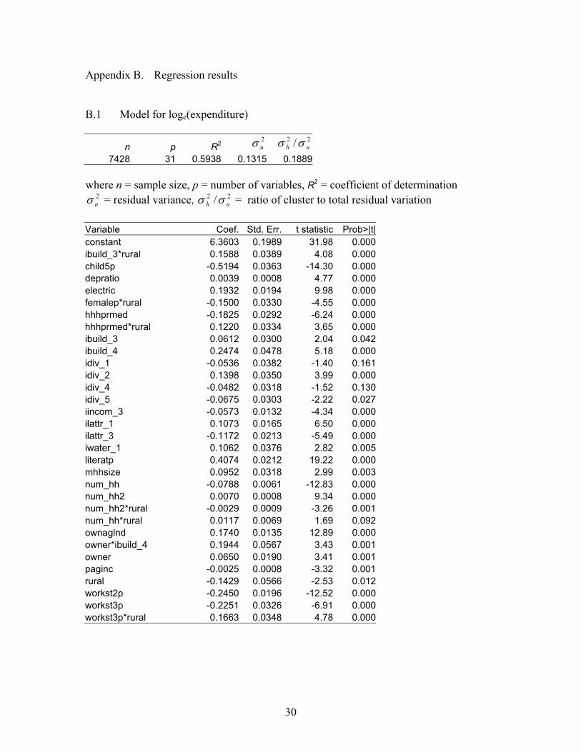
Appendix B. Regression results B.1 Model for loge(expenditure)

n p R2 2uσ 22 / uh σσ

7428 31 0.5938 0.1315 0.1889 where n = sample size, p = number of variables, R2 = coefficient of determination

2uσ = residual variance, = ratio of cluster to total residual variation 22 / uh σσ

Variable Coef. Std. Err. t statistic Prob>|t|constant 6.3603 0.1989 31.98 0.000ibuild_3*rural 0.1588 0.0389 4.08 0.000child5p -0.5194 0.0363 -14.30 0.000depratio 0.0039 0.0008 4.77 0.000electric 0.1932 0.0194 9.98 0.000femalep*rural -0.1500 0.0330 -4.55 0.000hhhprmed -0.1825 0.0292 -6.24 0.000hhhprmed*rural 0.1220 0.0334 3.65 0.000ibuild_3 0.0612 0.0300 2.04 0.042ibuild_4 0.2474 0.0478 5.18 0.000idiv_1 -0.0536 0.0382 -1.40 0.161idiv_2 0.1398 0.0350 3.99 0.000idiv_4 -0.0482 0.0318 -1.52 0.130idiv_5 -0.0675 0.0303 -2.22 0.027iincom_3 -0.0573 0.0132 -4.34 0.000ilattr_1 0.1073 0.0165 6.50 0.000ilattr_3 -0.1172 0.0213 -5.49 0.000iwater_1 0.1062 0.0376 2.82 0.005literatp 0.4074 0.0212 19.22 0.000mhhsize 0.0952 0.0318 2.99 0.003num_hh -0.0788 0.0061 -12.83 0.000num_hh2 0.0070 0.0008 9.34 0.000num_hh2*rural -0.0029 0.0009 -3.26 0.001num_hh*rural 0.0117 0.0069 1.69 0.092ownaglnd 0.1740 0.0135 12.89 0.000owner*ibuild_4 0.1944 0.0567 3.43 0.001owner 0.0650 0.0190 3.41 0.001paginc -0.0025 0.0008 -3.32 0.001rural -0.1429 0.0566 -2.53 0.012workst2p -0.2450 0.0196 -12.52 0.000workst3p -0.2251 0.0326 -6.91 0.000workst3p*rural 0.1663 0.0348 4.78 0.000

30

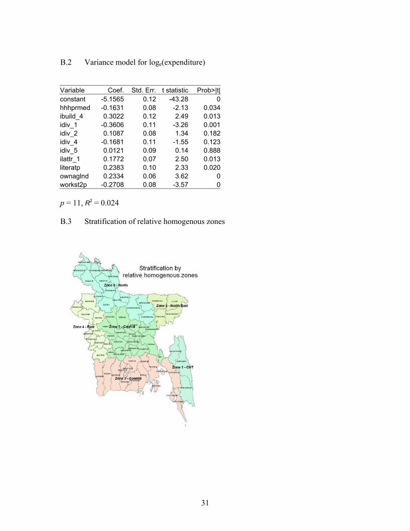
B.2 Variance model for loge(expenditure) Variable Coef. Std. Err. t statistic Prob>|t|constant -5.1565 0.12 -43.28 0hhhprmed -0.1631 0.08 -2.13 0.034ibuild_4 0.3022 0.12 2.49 0.013idiv_1 -0.3606 0.11 -3.26 0.001idiv_2 0.1087 0.08 1.34 0.182idiv_4 -0.1681 0.11 -1.55 0.123idiv_5 0.0121 0.09 0.14 0.888ilattr_1 0.1772 0.07 2.50 0.013literatp 0.2383 0.10 2.33 0.020ownaglnd 0.2334 0.06 3.62 0workst2p -0.2708 0.08 -3.57 0 p = 11, R2 = 0.024 B.3 Stratification of relative homogenous zones

31

B.4 Summary of models for loge(kilocalories)

n R2 p2uσ 22 / uh σσ

Zone1 60 0.2266 3 0.0311 0.1238Zone2 379 0.3096 13 0.0302 0Zone3 1887 0.3265 28 0.0351 0.1024Zone4 980 0.3048 27 0.0317 0.0281Zone5 2579 0.2155 22 0.0419 0.2341Zone6 1538 0.2968 26 0.0387 0.1117 B.5 Summary of models for height-for-age Mean Variance

n R2 p2uσ 22 / uh σσ R2 p

Zone1 29 0.3379 1 0.5874 0 0.1615 1 Zone2 261 0.1766 8 2.0801 0 0.0131 1 Zone3 936 0.1995 17 1.4862 0.0090 0.0148 4 Zone4 413 0.1210 10 1.1580 0.0018 0.0160 3 Zone5 1172 0.1699 13 1.5541 0.0355 0.0253 4 Zone6 750 0.1299 10 1.4554 0.0309 0.0568 9 B.6 Summary of models for weight-for-age Mean Variance

n R2 p2uσ 22 / uh σσ R2 p

Zone1 29 0.1758 1 0.7195 0 0.0506 1 Zone2 261 0.1806 11 0.9584 0 0.0728 6 Zone3 936 0.1048 10 0.8581 0.0301 0.0023 1 Zone4 413 0.1318 7 0.7609 0.0096 0.1002 8 Zone5 1172 0.1488 10 0.8493 0.0802 0.0059 1 Zone6 750 0.0953 10 0.7511 0.0310 0.0152 5

32

Appendix C. Summary of small-area estimates C.1 Comparison of division-level poverty measures Div1 HIES se LCL UCL SAE seP0l 0.2632 0.0326 0.1993 0.3272 0.3023 0.0252P1l 0.0483 0.0080 0.0320 0.0645 0.0660 0.0079P2l 0.0130 0.0029 0.0070 0.0189 0.0209 0.0031P0u 0.3752 0.0388 0.2992 0.4513 0.4166 0.0268P1u 0.0824 0.0106 0.0608 0.1040 0.1046 0.0102P2u 0.0252 0.0042 0.0166 0.0338 0.0370 0.0046Div2 HIES se LCL UCL SAE seP0l 0.2263 0.0202 0.1866 0.2659 0.2338 0.0109P1l 0.0433 0.0052 0.0329 0.0537 0.0506 0.0032P2l 0.0121 0.0018 0.0085 0.0157 0.0162 0.0012P0u 0.4403 0.0237 0.3938 0.4869 0.3949 0.0127P1u 0.1045 0.0083 0.0880 0.1209 0.1050 0.0049P2u 0.0351 0.0036 0.0280 0.0423 0.0389 0.0023Div3 HIES se LCL UCL SAE seP0l 0.2802 0.0193 0.2422 0.3181 0.2513 0.0139P1l 0.0608 0.0055 0.0499 0.0717 0.0568 0.0045P2l 0.0190 0.0022 0.0146 0.0234 0.0187 0.0018P0u 0.4045 0.0212 0.3629 0.4461 0.3534 0.0151P1u 0.1019 0.0071 0.0879 0.1158 0.0909 0.0058P2u 0.0353 0.0031 0.0293 0.0413 0.0329 0.0026Div4 HIES se LCL UCL SAE seP0l 0.2833 0.0248 0.2347 0.3319 0.2684 0.0200P1l 0.0498 0.0058 0.0381 0.0615 0.0600 0.0061P2l 0.0132 0.0019 0.0094 0.0171 0.0195 0.0024P0u 0.4423 0.0329 0.3778 0.5067 0.4040 0.0222P1u 0.1035 0.0094 0.0846 0.1223 0.1079 0.0087P2u 0.0330 0.0036 0.0259 0.0402 0.0401 0.0040Div5 HIES se LCL UCL SAE seP0l 0.3999 0.0223 0.3563 0.4435 0.3810 0.0149P1l 0.0982 0.0083 0.0817 0.1147 0.0954 0.0058P2l 0.0341 0.0038 0.0265 0.0417 0.0337 0.0026P0u 0.5189 0.0216 0.4766 0.5612 0.5060 0.0145P1u 0.1511 0.0100 0.1313 0.1708 0.1471 0.0070P2u 0.0587 0.0052 0.0483 0.0691 0.0579 0.0036 P0l = lower poverty incidence, P0u = upper poverty incidence, P1l = lower poverty gap, etc.

33

C.2 Summary of upazila-level poverty measures # Obs Mean Std. Dev. Min MaxP0l 507 0.2930 0.1063 0.0014 0.5531seP0l 507 0.0388 0.0146 0.0025 0.1145p0u 507 0.4212 0.1238 0.0049 0.7081seP0u 507 0.0416 0.0143 0.0062 0.1081P1l 507 0.0679 0.0297 0.0001 0.1638seP1l 507 0.0127 0.0054 0.0003 0.0436P1u 507 0.1142 0.0421 0.0006 0.2441seP1u 507 0.0169 0.0066 0.0009 0.0538P2l 507 0.0228 0.0112 0.0000 0.0650seP2l 507 0.0055 0.0026 0.0001 0.0203P2u 507 0.0429 0.0182 0.0001 0.1091seP2u 507 0.0082 0.0036 0.0002 0.0300 seP0l = standard error lower poverty incidence, seP0u = std err upper poverty incidence, P1l = std err lower poverty gap, etc.

34

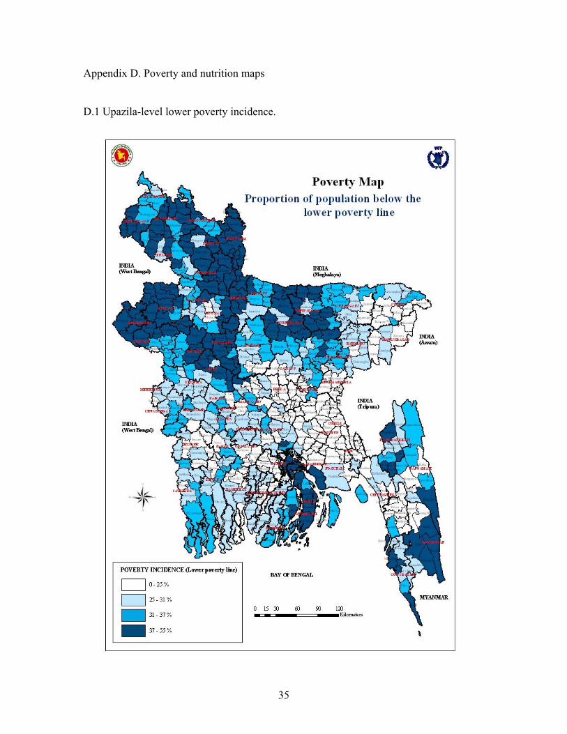
Appendix D. Poverty and nutrition maps D.1 Upazila-level lower poverty incidence.

35

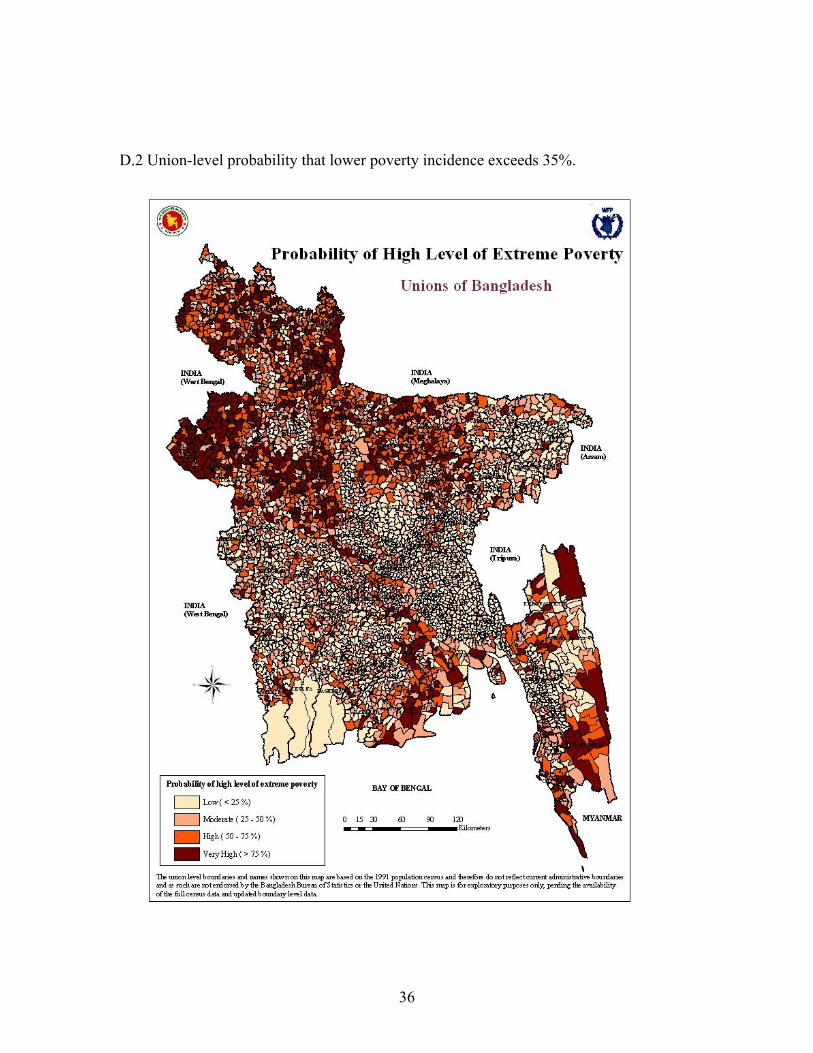
D.2 Union-level probability that lower poverty incidence exceeds 35%.

36

D.3 Upazila-level resource requirements

37

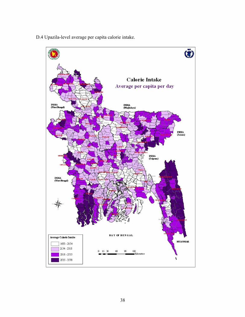
D.4 Upazila-level average per capita calorie intake.

38

D.5 Upazila-level incidence of hard-core food poverty.

39

D.6 Upazila-level incidence of stunting.

40

D.7 Upazila-level probability of stunting > 50%.

41

D.8 Upazila-level incidence of underweight.

42

D.9 Upazila-level probability of underweight > 50%.

43