LOCAL ENVIRONMENTAL REGULATION AND PLANT-LEVEL

LOCAL ENVIRONMENTAL REGULATION AND

PLANT-LEVEL PRODUCTIVITY

By

Randy A. Becker*

U.S. Bureau of the Census

CES 10-30R August, 2011 This paper is a revised version of “Local Environmental Regulation and Plant-Level Productivity” (CES-WP-10-30) from August 2011. A copy of the original paper is available upon request. The research program of the Center for Economic Studies (CES) produces a wide range of economic analyses to improve the statistical programs of the U.S. Census Bureau. Many of these analyses take the form of CES research papers. The papers have not undergone the review accorded Census Bureau publications and no endorsement should be inferred. Any opinions and conclusions expressed herein are those of the author(s) and do not necessarily represent the views of the U.S. Census Bureau. All results have been reviewed to ensure that no confidential information is disclosed. Republication in whole or part must be cleared with the authors. To obtain information about the series, see www.census.gov/ces or contact Cheryl Grim, Editor, Discussion Papers, U.S. Census Bureau, Center for Economic Studies 2K130B, 4600 Silver Hill Road, Washington, DC 20233, [email protected].

http://www.census.gov/ces�

mailto:[email protected]�

Abstract

This paper examines the impact of environmental regulation on the productivity of manufacturing plants in the United States. Establishment-level data from three Censuses of Manufactures are used to estimate 3-factor Cobb-Douglas production functions that include a measure of the stringency of environmental regulation faced by manufacturing plants. In contrast to previous studies, this paper examines effects on plants in all manufacturing industries, not just those in “dirty” industries. Further, this paper employs spatial-temporal variation in environmental compliance costs to identify effects, using a time-varying county-level index that is based on multiple years of establishment-level data from the Pollution Abatement Costs and Expenditures survey and the Annual Survey of Manufactures. Results suggest that, for the average manufacturing plant, there is no statistically significant effect on productivity of being in a county with higher environmental compliance costs. For the average plant, the main effect of environmental regulation may not be in the spatial and temporal dimensions. Keywords: environmental regulation, productivity, U.S. manufacturing

* Forthcoming in Ecological Economics. This paper has benefited from the helpful comments of three anonymous referees, Jim Davis, Lucia Foster, Wayne Gray, and participants at the Fourth World Congress of Environmental and Resource Economists. Any opinions and conclusions expressed herein are those of the author and do not necessarily represent the views of the U.S. Census Bureau. All results have been reviewed to ensure that no confidential information is disclosed.

1. Introduction

This paper examines the impact of environmental regulation on the productivity of

manufacturing plants in the United States. At the facility level, environmental regulation may

affect productivity in at least two ways. First, compliance may require the diversion of inputs –

capital, labor, materials, etc. – toward the production of (unmeasured) environmental quality.

Second, regulation may necessitate changes in the production process, reducing efficiency (as

traditionally defined). At a more aggregate level, environmental regulation may affect

productivity by exempting existing plants from the most stringent standards. This can

discourage entry of new, more efficient producers.

A number of studies have attempted to measure the effects of environmental regulation on

aggregate productivity (i.e., at the national, sectoral, or industry level), particularly on the

productivity slowdown of the 1970s (see Jaffe et al. 1995 for a review). Gray (1987) examines

productivity growth in 450 manufacturing industries (4-digit SIC industries) between 1958 and

1978 and finds that, for the average manufacturing industry, about 12% of the 1970s productivity

decline is attributable to environmental regulation – an estimate that does not achieve statistical

significance. Barbera and McConnell (1986) focus on four particularly polluting (and regulated)

manufacturing sectors (2- to 3-digit SIC industries) between 1960 and 1980 and find that

pollution abatement requirements reduced both average labor productivity growth and capital

productivity growth in the chemical and primary metal sectors, but not in paper. It further

appears that environmental regulation is responsible for a large portion of the productivity

slowdown after 1973. In another study, analyzing these same manufacturing sectors, the same

authors find that environmental regulations reduced the productivity growth rate between 9% and

55%, accounting for 10% to 30% of the 1970s productivity decline (Barbera and McConnell

1990).

A more limited number of studies have examined facility-level productivity, as I do here.

For example, Gollop and Roberts (1983) find that electric utilities subject to greater restrictions

on their sulfur dioxide emissions had lower productivity growth rates. Gray and Shadbegian

(1995) find that $1 of additional expenditure on pollution abatement reduced facility output by

more than $1 – upwards of $3.28 for plants in the steel industry. In a more recent study, these

same authors find that pollution abatement expenditure reduced productivity by 9.3% in

“integrated” paper mills (i.e., ones that also produce pulp) and only 0.9% in non-integrated mills

(Gray and Shadbegian 2003). In their study of integrated paper mills, Boyd and McClelland

(1999) find a nearly identical reduction in productivity due to environmental constraints.

Meanwhile, Shadbegian and Gray (2005) find few statistically significant effects (positive or

negative) of pollution abatement expenditures (capital, labor, or materials) on the productivity of

paper mills, petroleum refineries, and steel plants.

In contrast to these other studies that also use facility-level data, I examine effects on plants

in all manufacturing industries, not just those in “dirty” industries, such as electric utilities, steel,

petroleum refining, and paper. Here, I employ establishment-level data from three Censuses of

Manufactures (CMs) to estimate 3-factor Cobb-Douglas production functions. While these

previous studies use a facility-specific measure of regulatory stringency, I employ spatial-

temporal variation in environmental compliance costs, in the form of a newly developed county-

level index that reveals extra-normal environmental compliance costs, generally due to above- or

below-normal environmental regulation and enforcement faced by manufacturers at the county

level. This index is based on establishment-level data from multiple years of the Pollution

Abatement Costs and Expenditures (PACE) survey and the Annual Survey of Manufactures

(ASM).

Results suggest that, for the average manufacturing plant, there is no statistically

significant effect on productivity of being in a county with higher environmental compliance

costs. The paper proceeds as follows. Section 2 discusses the time-varying county-level index

of environmental compliance costs, and Section 3 discusses the data and empirical specification

used in the productivity analyses. Section 4 presents results, and Section 5 offers some

concluding remarks.

2. A Time-varying County-level Index of Environmental Compliance Costs

In this paper, I use spatial and temporal variation in environmental compliance costs to

examine the effects of environmental regulation on productivity. This variation is measured by a

county-level index of the sort introduced and discussed in Becker (2011). In particular, I employ

the establishment-level data from the PACE surveys of 1980-1982, 1984-1986, and 1988-1994,

which includes data on total pollution abatement operating costs (PAOC).1

1 These survey data, as well as those from the Annual Survey of Manufactures and the Census of Manufactures, are confidential, collected and protected under Title 13 of the U.S. Code. Restricted access to these data can be arranged through the U.S. Census Bureau’s Center for Economic Studies. See http://www.census.gov/ces/ for details.

PAOC includes

salaries & wages, parts & materials, fuel & electricity, capital depreciation, contract work,

equipment leasing, and other operating costs associated with a plant’s abatement of its air and

water pollution as well as its solid waste in that calendar year. To this I merge data on these

establishments from the ASM or CM, including employment, value of shipments, four-digit SIC

industry, county, and plant vintage (as measured by an establishment’s first appearance in the

Census of Manufactures). After restricting the sample to cases that had linkable PACE and

ASM/CM records in a given year, and after eliminating inactive establishments, plants in Alaska

and Hawaii, and those with missing or incomplete data on critical items, there are 188,326

establishment-years of observations for estimating the county-level index.

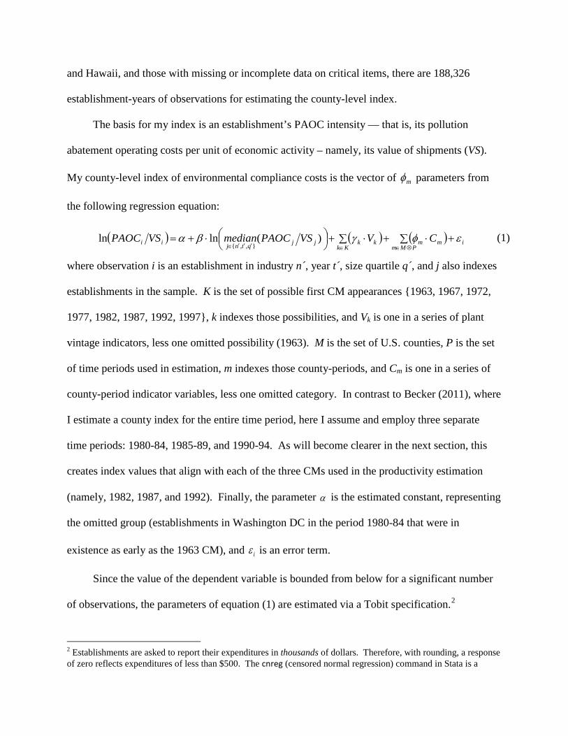
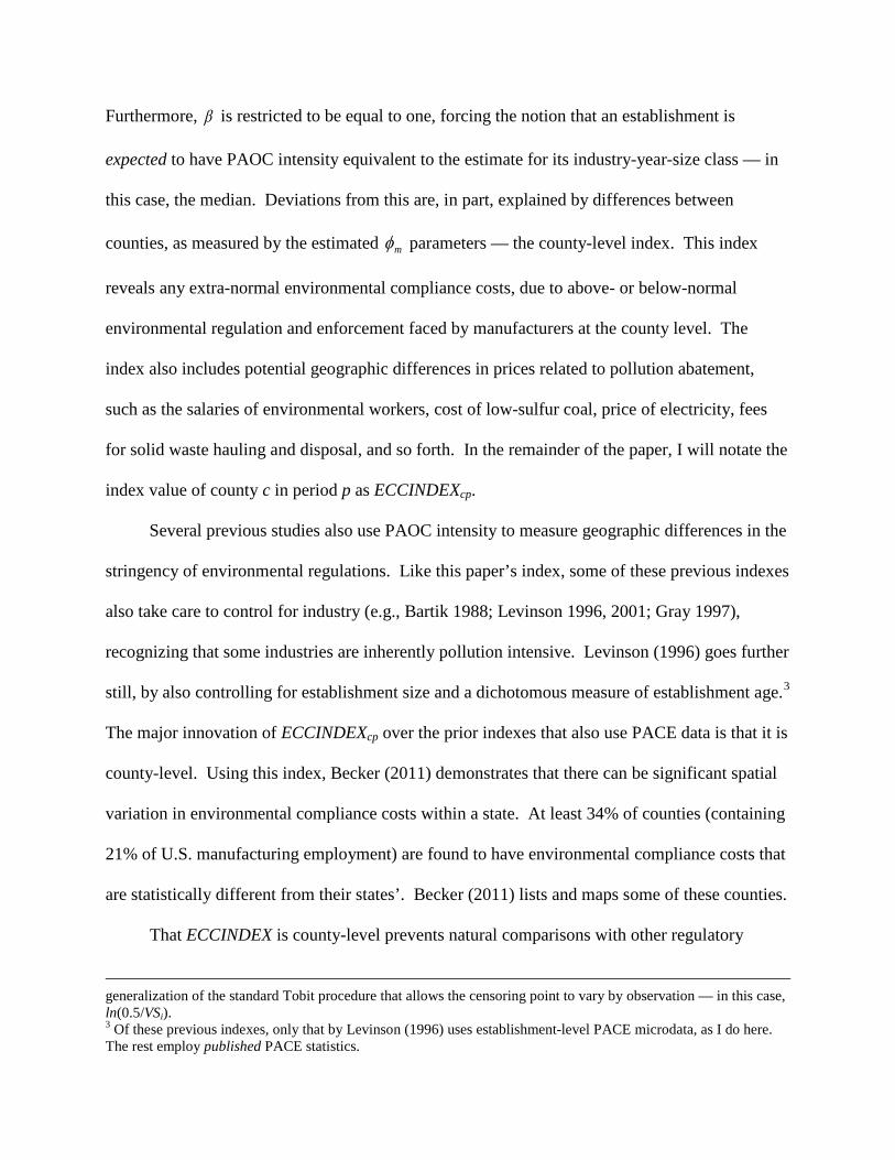
The basis for my index is an establishment’s PAOC intensity — that is, its pollution

abatement operating costs per unit of economic activity – namely, its value of shipments (VS).

My county-level index of environmental compliance costs is the vector of mφ parameters from

the following regression equation:

( ) ( ) ( ) iPMm

mmKk

kkjjqtnjii CVVSPAOCmedianVSPAOC εφγβα +∑ ⋅+∑ ⋅+

⋅+=

⊗∈∈′′′∈)(lnln

},,{ (1)

where observation i is an establishment in industry n´, year t´, size quartile q´, and j also indexes

establishments in the sample. K is the set of possible first CM appearances {1963, 1967, 1972,

1977, 1982, 1987, 1992, 1997}, k indexes those possibilities, and Vk is one in a series of plant

vintage indicators, less one omitted possibility (1963). M is the set of U.S. counties, P is the set

of time periods used in estimation, m indexes those county-periods, and Cm is one in a series of

county-period indicator variables, less one omitted category. In contrast to Becker (2011), where

I estimate a county index for the entire time period, here I assume and employ three separate

time periods: 1980-84, 1985-89, and 1990-94. As will become clearer in the next section, this

creates index values that align with each of the three CMs used in the productivity estimation

(namely, 1982, 1987, and 1992). Finally, the parameter α is the estimated constant, representing

the omitted group (establishments in Washington DC in the period 1980-84 that were in

existence as early as the 1963 CM), and iε is an error term.

Since the value of the dependent variable is bounded from below for a significant number

of observations, the parameters of equation (1) are estimated via a Tobit specification.2

2 Establishments are asked to report their expenditures in thousands of dollars. Therefore, with rounding, a response of zero reflects expenditures of less than $500. The cnreg (censored normal regression) command in Stata is a

Furthermore, β is restricted to be equal to one, forcing the notion that an establishment is

expected to have PAOC intensity equivalent to the estimate for its industry-year-size class — in

this case, the median. Deviations from this are, in part, explained by differences between

counties, as measured by the estimated mφ parameters — the county-level index. This index

reveals any extra-normal environmental compliance costs, due to above- or below-normal

environmental regulation and enforcement faced by manufacturers at the county level. The

index also includes potential geographic differences in prices related to pollution abatement,

such as the salaries of environmental workers, cost of low-sulfur coal, price of electricity, fees

for solid waste hauling and disposal, and so forth. In the remainder of the paper, I will notate the

index value of county c in period p as ECCINDEXcp.

Several previous studies also use PAOC intensity to measure geographic differences in the

stringency of environmental regulations. Like this paper’s index, some of these previous indexes

also take care to control for industry (e.g., Bartik 1988; Levinson 1996, 2001; Gray 1997),

recognizing that some industries are inherently pollution intensive. Levinson (1996) goes further

still, by also controlling for establishment size and a dichotomous measure of establishment age.3

That ECCINDEX is county-level prevents natural comparisons with other regulatory

The major innovation of ECCINDEXcp over the prior indexes that also use PACE data is that it is

county-level. Using this index, Becker (2011) demonstrates that there can be significant spatial

variation in environmental compliance costs within a state. At least 34% of counties (containing

21% of U.S. manufacturing employment) are found to have environmental compliance costs that

are statistically different from their states’. Becker (2011) lists and maps some of these counties.

generalization of the standard Tobit procedure that allows the censoring point to vary by observation — in this case, ln(0.5/VSi). 3 Of these previous indexes, only that by Levinson (1996) uses establishment-level PACE microdata, as I do here. The rest employ published PACE statistics.

indexes. Nevertheless, the index is positively and significantly correlated with a number of state-

level indexes produced by environmental organizations, including a +0.48 correlation with the

state ranking based on the League of Conservation Voters (LCV) “scorecard” on each member of

Congress.4 The states with highest index values tend to be in the northeast.5

ECCINDEX is also found to be positively correlated with certain county characteristics,

including population (and population density), manufacturing employment, per capita income,

and dichotomous indicators of non-attainment of the Clean Air Act’s national ambient air quality

standards (NAAQS) for each the six “criteria” air pollutants. Since these county characteristics

are also significantly correlated with each other, a simple OLS regression is used to examine

their independent impacts. Results suggest that, all else being equal, county population has a

negative effect on ECCINDEX, manufacturing employment has a positive effect, NAAQS non-

attainment has a positive effect, and (mostly in specifications with state fixed effects) county per

capita income has a positive effect.

The states with the

lowest index values tend to be Great Plains states.

6

4 Here, I create a state-level index by taking a weighted average of the county-level indexes in the state, where the weight is the county’s share of the state’s manufacturing employment. The Spearman rank correlation between this state-level index (based on ECCINDEX) and the states’ ranking according to the LCV’s National Environmental Scorecard for years 1977-1994 (as constructed by Levinson 2001) is +0.4783. The ECCINDEX-based state-level index is also significantly correlated with the state-level FREE index (+0.29), the Levinson 1996 index (+0.28), and the Hall-Kerr Green Index (+0.27), as republished in Levinson (2001).

It is worth noting that ECCINDEX’s correlation with the

county NAAQS non-attainment statuses, while positive, is relatively small (+0.12). This is

perhaps not unexpected since the index here captures expenditures on the abatement of air

pollutants beside the six criteria pollutants, as well as the abatement of water pollution and solid

5 Again using the state-level index that is a weighted average of the county-level indexes in the state, the top ten is dominated by New England and Mid-Atlantic states. Interestingly, the top 20 contains all 17 of the contiguous states east of (and including) Illinois and Michigan, and north of (and including) Kentucky, West Virginia, and Maryland. 6 Results depend somewhat on the exact specification – e.g., which of two formulations for ECCINDEX is employed, whether or not observations are weighted by a county’s manufacturing employment, whether or not state effects are include, and so forth. Here I report the most frequently occurring results.

waste.7 Analyses on county-level indexes of the separate components of ECCINDEX suggest

that the spatial variation in environmental compliance costs is greatest for air and water, and that

ECCINDEX is most closely correlated with the index for solid waste. In terms of cost categories,

ECCINDEX is found to be most closely correlated with the cost indexes for

materials/supplies/fuel/electricity and for salaries/wages, both of which vary less than other

components of costs.8

To provide a sense of the cost differentials that are implied by ECCINDEX, I consider the

difference between the 75th and 25th percentiles of its value. On average, all else being equal,

plants located in the county with the higher index value would have pollution abatement

operating costs that are about 198% higher.

9 According to data published by the U.S. Census

Bureau, in 1992, there were approximately 370,900 manufacturing establishments, and they had

approximately $17.5 billion in PAOC, for an average of about $47,000 per manufacturing

establishment.10

7 During the period 1980-1994, the share of PAOC devoted to air, water, and solid waste was 33%, 38%, and 29%, respectively. Becker (2004) has also shown that certain populations can impact the pollution abatement expenditure of local manufacturers, over and above any “formal” regulatory requirements arising from county NAAQS non-attainment and from other state and federal regulation.

A 198% difference is roughly $93,000, which, for the average manufacturing

plant in 1992, was about 1.15% of its annual shipments (revenue) and 2.42% of its value added.

Considering where manufacturing activity actually takes place, by weighting each county by its

total manufacturing employment, all else equal, plants in the county at the 75th percentile would

have pollution abatement operating costs that are about 65% higher than those for plants in the

county at the 25th percentile — a difference of about $30,500 for the average manufacturing

8 These analyses are complicated by the fact that the PACE survey altered the categorization of costs during this period, such that labor and depreciation are the only two categories with completely consistent definitions. 9 There is uncertainty surrounding this difference, since index values toward the extremes tend to be less precisely estimated (i.e., tend to have higher standard errors, are based on fewer underlying observations). The precision of the index values is considered later in the paper. 10 In actuality, the aggregate PAOC figure is for establishments with 20 or more employees, of which there were approximately 119,000 in 1992. Establishments with fewer than 20 employees tend to be in less-polluting industries and therefore have relatively small pollution abatement expenditure.

plant in 1992, or about 0.38% of its annual revenue and 0.79% of its value added. This of course

hides significant industry heterogeneity. For example, the average pulp mill (SIC 2611) had

roughly $6.5 million of PAOC in 1992 – or about 138 times more than the average

manufacturing plant. Moreover, a 65% difference was about 3.5% of the annual revenue for the

average plant in this industry and 7.4% of its value added.

3. Productivity Data and Empirical Specification

Data to estimate plant-level productivity come from the CMs of 1982, 1987, and 1992,

which include data on establishment employment, value of output, capital assets, material usage,

location, industry, age, ownership, and so forth. After eliminating establishments that exhibited

signs of inactivity (i.e., had a zero value for one or more critical items), whose data were largely

imputed, and/or that were located in counties with no index, I am left with nearly 568,000 plant-

years of observations.

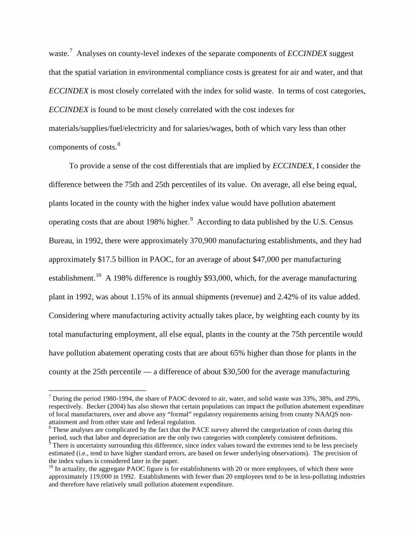
To examine the effect of environmental compliance costs on manufacturers’ productivity, I

estimate some traditional Cobb-Douglas production functions. In particular, I estimate 3-factor

Cobb-Douglas labor productivity regressions, one of which includes:

itcicnitntt

aitaititit

itititit

itctcpitit

eCOUNTYSICYEARAGEMULTIEMPNPWEMP

EMPrMATEMPCAPITALEMPCOUNTYMFGECCINDEXEMPrVS

+⋅+⋅+⋅+⋅+⋅+⋅

+⋅+⋅+⋅+⋅+⋅+=

∑∑∑∑

λλλλλλ

λλλλλλ

76

54

3210

)/log()/log()/log(

)log()log()/log(

(2)

where, for plant i at time t in county c, rVS is output (the real value of shipments), EMP is the

total number of employees, ECCINDEX is the time-varying county-level index of environmental

compliance costs (as defined in the previous section), COUNTYMFG is time-varying county-

level manufacturing employment, CAPITAL is the book value of capital assets, rMAT is the real

value of material inputs, NPWEMP is the number of non-production workers (and

NPWEMP/EMP measures the proportion of the workforce that was not engaged in production –

a commonly used measure of “skill” mix), MULTI is a dummy variable indicating a plant

belonged to a multi-establishment firm, AGE is a series of five categorical variables to designate

the plant’s age/vintage (less one omitted category), YEAR is a set of year dummies, SIC is a set

of dummy variables indicating the plant’s four-digit SIC industry, and COUNTY is a set of

dummy variables indicating the plant’s county. Industry-specific deflators, to create constant-

dollar values for both value of shipments (VS) and value of material inputs (MAT), come from

the NBER-CES Manufacturing Industry Database.11

Note that equation (2) controls for time-invariant location effects. This can be important if

there are such fixed effects (observed or unobserved) that are correlated with both manufacturing

plant productivity and the variable of interest, ECCINDEX. Indeed, ECCINDEX is found to have

a statistically significant (positive) correlation with county characteristics such as total

population, industrial concentration in manufacturing, and being in a metropolitan area, which

may have impacts on plant productivity. The equation also controls for time-varying county

manufacturing employment, COUNTYMFG, which measures changing “economies of

agglomeration” as manufacturing activity increases or declines in a county. Such a measure also

proxies for any observable and unobservable characteristics of a county that vary over time,

contribute to productivity, and lead manufacturers to increase or decrease their activity there. In

other words, if some county characteristic changes, and if it has an effect on manufacturers’

productivity, it would also presumably affect the level of manufacturing activity in the county,

which COUNTYMFG measures.

12

11 The latest version of this database is available at http://www.nber.org/data/nbprod2005.html.

12 I have examined whether adding time-varying county-level population to specifications matters. It has no

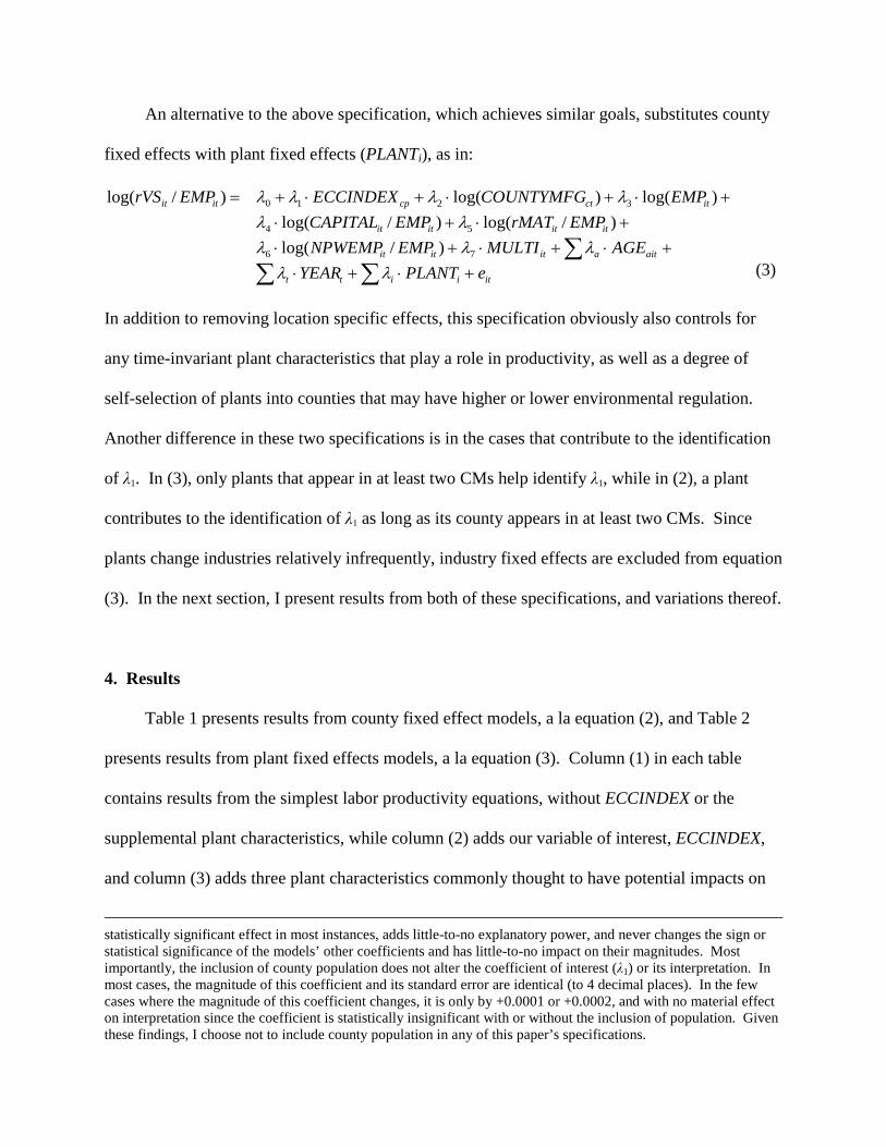
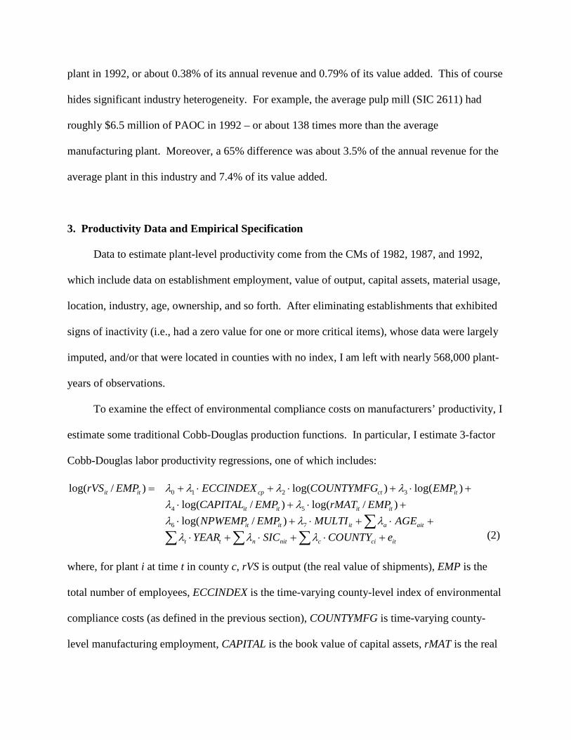
An alternative to the above specification, which achieves similar goals, substitutes county

fixed effects with plant fixed effects (PLANTi), as in:

itiitt

aitaititit

itititit

itctcpitit

ePLANTYEARAGEMULTIEMPNPWEMP

EMPrMATEMPCAPITALEMPCOUNTYMFGECCINDEXEMPrVS

+⋅+⋅+⋅+⋅+⋅

+⋅+⋅+⋅+⋅+⋅+=

∑∑∑

λλλλλ

λλλλλλ

76

54

3210

)/log()/log()/log(

)log()log()/log(

(3)

In addition to removing location specific effects, this specification obviously also controls for

any time-invariant plant characteristics that play a role in productivity, as well as a degree of

self-selection of plants into counties that may have higher or lower environmental regulation.

Another difference in these two specifications is in the cases that contribute to the identification

of λ1. In (3), only plants that appear in at least two CMs help identify λ1, while in (2), a plant

contributes to the identification of λ1 as long as its county appears in at least two CMs. Since

plants change industries relatively infrequently, industry fixed effects are excluded from equation

(3). In the next section, I present results from both of these specifications, and variations thereof.

4. Results

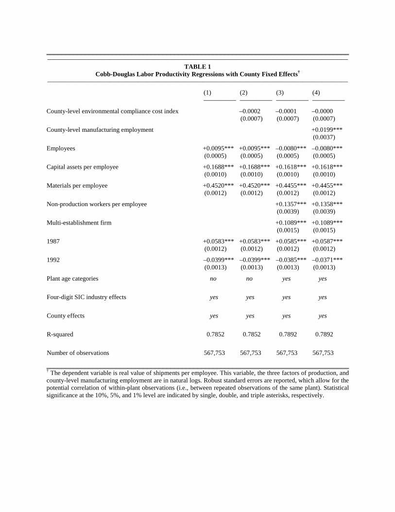
Table 1 presents results from county fixed effect models, a la equation (2), and Table 2

presents results from plant fixed effects models, a la equation (3). Column (1) in each table

contains results from the simplest labor productivity equations, without ECCINDEX or the

supplemental plant characteristics, while column (2) adds our variable of interest, ECCINDEX,

and column (3) adds three plant characteristics commonly thought to have potential impacts on

statistically significant effect in most instances, adds little-to-no explanatory power, and never changes the sign or statistical significance of the models’ other coefficients and has little-to-no impact on their magnitudes. Most importantly, the inclusion of county population does not alter the coefficient of interest (λ1) or its interpretation. In most cases, the magnitude of this coefficient and its standard error are identical (to 4 decimal places). In the few cases where the magnitude of this coefficient changes, it is only by +0.0001 or +0.0002, and with no material effect on interpretation since the coefficient is statistically insignificant with or without the inclusion of population. Given these findings, I choose not to include county population in any of this paper’s specifications.

productivity (NPWEMP/EMP, MULTI, and AGE). Finally, column (4) of each table contains

results from the (full) models specified in equations (2) and (3), respectively, which include

time-varying county-level manufacturing employment (COUNTYMFG).

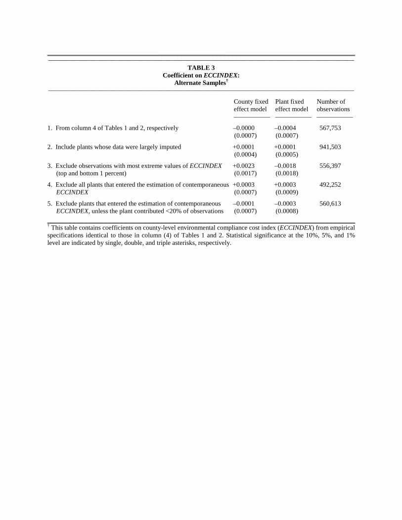
In none of the specifications of Table 1 or Table 2 does ECCINDEX have a statistically

significant effect on productivity. Table 3 evaluates the robustness of these results, employing

several alternate samples. Sample 2 includes plants, previously excluded, whose data were

largely imputed. Sample 3 eliminates establishments in the top and bottom 1% of ECCINDEX,

to assess whether extreme cases are influencing results. Neither of these samples changes the

basic conclusion, though in the latter case, the point estimates do change a fair amount, but are

nonetheless statistically insignificant. Endogeneity may be a concern in these analyses, since

plants in the productivity regressions may also be in the sample used to estimate ECCINDEX.

Sample 4 treats this by excluding all plants that entered the estimation of (contemporaneous)

ECCINDEX. The point estimates are a bit higher but statistically insignificant. Sample 4 is

rather unforgiving – eliminating 13.3% of the sample (relative to Sample 1), including many

“important” plants, as well as ones located in counties with extensive manufacturing activity,

where a single plant has little likelihood of dominating the estimated ECCINDEX. Sample 5

instead eliminates plants that entered the estimation of ECCINDEX, but only if the plant

contributed at least 20% of the underlying observations in that county-period.13 Again,

ECCINDEX has no statistically significant effect on productivity. Meanwhile, the coefficients

on the models’ other variables are as one might expect.14

13 Cutoffs of 10% and 5% were also chosen, yielding the same essential conclusion.

14 A labor productivity equation in the form of (Q/L)=A·Lα+β+γ-1(K/L)β(M/L)γ is derived from a standard Cobb-Douglas production function of the form Q=A·LαKβMγ. The coefficient on log(EMP), therefore, is α+β+γ –1. Therefore, column 4 of Table 1 [2] shows output elasticities on labor, capital, and materials of 0.385, 0.162, and 0.446, [0.459, 0.097, and 0.346], respectively, with statistically significant decreasing returns to scale in both instances. Meanwhile, the skill measure and multi-establishment status are both found to have statistically

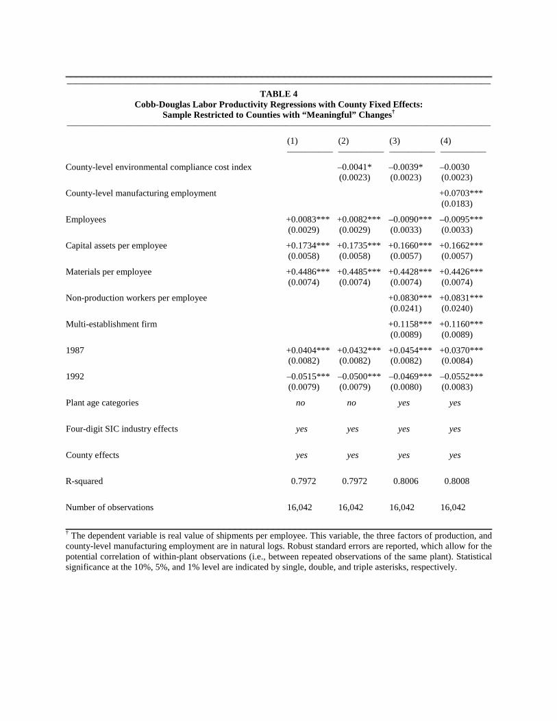
These results suggest that the average manufacturing plant does not have lower

productivity in counties with higher environmental compliance costs. One possible issue with

these specifications is that the effect of ECCINDEX is identified only by changes within a

county, for counties or plants that appear more than once. If much of the variation in

ECCINDEX is cross-sectional (i.e., across counties, rather than over time), and if there is

measurement error in ECCINDEX (and the estimation of equation (1) does yield a standard error

on each index value), then controlling for county or plant fixed effects may leave relatively little

“true” variation in ECCINDEX, which may bias its coefficient toward zero. Indeed, I find that of

the 2,059 counties with an ECCINDEX for both the period 1980-84 and 1990-94, only 206

experienced a statistically meaningful change between those two periods.15,16

First, I re-estimate the models of Tables 1 and 2, using only those plants in counties with

statistically meaningful changes in their ECCINDEX.

With this in mind,

I present results from two further exercises.

17

significant positive effects on labor productivity, and county manufacturing employment also has a statistically significant positive effect, as expected.

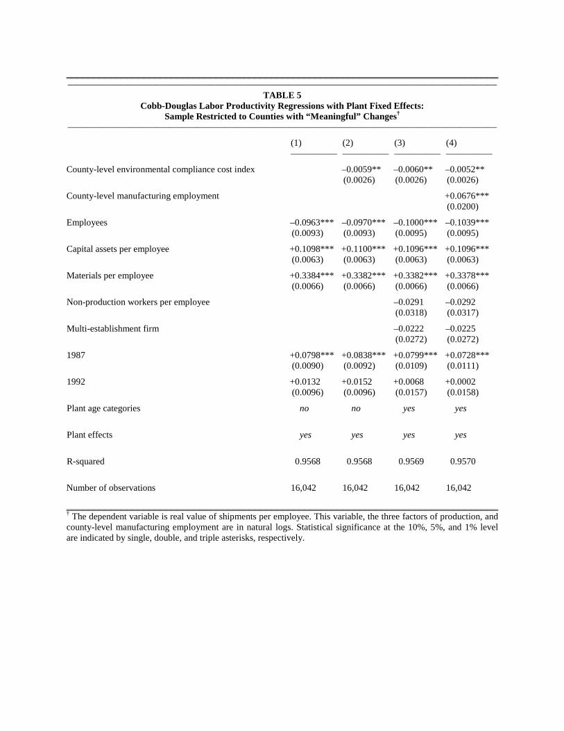
The results are presented in Tables 4 and

5, respectively. In the county fixed effect models (Table 4), ECCINDEX has a statistically

significant (negative) effect on productivity, until county-level manufacturing employment is

added to the specification in column 4. In the plant fixed effect models (Table 5), ECCINDEX

15 In particular, I test whether the 90% confidence interval of the difference in the index values excludes zero. The formula allows some overlap of the confidence intervals of the two individual index values (Schenker and Gentleman 2001). 16 No major manufacturing counties are among these 206, and collectively they contain less than 3% of U.S. manufacturing employment. An alternate specification of ECCINDEX yields a similar result. Namely, specification #6 in Becker (2011) uses: (i) plant employment (EMP) in the denominator of PAOC intensity (and expected PAOC intensity), instead of value of shipments (VS), and (ii) the weighted mean in computing expected PAOC intensity, instead of median. With this index, I find that 256 counties – containing 4% of U.S. manufacturing employment – experienced a statistically meaningful change between those two periods. 17 In particular, for each county, I perform pairwise tests between the index values in 1982 & 1987, 1987 & 1992, and 1982 & 1992. If there are no statistically meaningful differences between any of the three pairs, the county and all of its plants are dropped from the sample. If only one statistically meaningful difference is found (e.g., between 1982 & 1992), then only observations in the remaining year are dropped (in this example, 1987). If two statistically meaningfully differences are found (e.g., between 1982 & 1992 and 1987 & 1992), all years and observations are retained.

has a statistically significant (negative) effect in all specifications.18,19 To help interpret the λ1

coefficient in column 4, I compute the effect on labor productivity for the plant experiencing the

average [and median] change in ECCINDEX, among those plants contributing to the

identification of this coefficient in these two regressions. In the county fixed effect regression,

the average [median] plant experienced an increase in ECCINDEX between its first and last year

of appearance that translates into a decrease in labor productivity of -0.08% [-0.40%], which for

the average [median] plant here reflects a decrease in output per worker of $88 [$280] in 1987

dollars. In the plant fixed effect regression, the average [median] plant experienced a decrease in

labor productivity of -0.09% [-0.32%], which for the average [median] plant in that sample

reflects a decrease in output per worker of $101 [$229] in 1987 dollars.20

Second, I estimate versions of equation (2) that employ 179 BEA economic area fixed

effects (Johnson and Kort 2004) instead of county fixed effects. This allows for some cross-

sectional variation in ECCINDEX while still controlling for local unobservables to a certain

degree. Results appear in Table 6. We see that the effect of ECCINDEX is not statistically

significant, though it is nearly so (p=0.118) in column (4). To help interpret this particular point

estimate, I compute the effect on labor productivity of moving from the 25th percentile of

ECCINDEX in this sample to the 75th percentile, holding all other variables constant. The effect

18 The endogeneity issue discussed above may be more of a concern here, since the counties in this sample appear to have less manufacturing activity than average and therefore a particular plant may be more likely to dominate the estimated ECCINDEX. Re-estimating the models of Table 4 and 5, using a sample that – like Sample 5 above – eliminates plants that entered the estimation of ECCINDEX but only if the plant contributed at least 20% of the underlying observations in that county-period (N=14,993), yields negative coefficients on ECCINDEX that are 50% to 75% the magnitude of those in Tables 4 and 5, and that do not quite achieve statistical significance. 19 I also estimate these regressions using the aforementioned alternative specification of ECCINDEX that uses EMP in the denominator of (expected) PAOC intensity, instead of VS, and uses weighted mean in computing expected PAOC intensity, instead of median. This ECCINDEX has no statistically significant effect in any of the regressions of Tables 4 or 5, or in the regressions of Tables 1, 2, and 6 for that matter. 20 Though unjustified, given the statistically insignificant results found elsewhere, extrapolating these particular results to the entire manufacturing sector, which had 17.7 million employees in 1987, yields estimates of lost output ranging from $1.6 to $5.0 billion in 1987 dollars, assuming $88 and $280 per worker, respectively. At this time, pollution abatement operating costs for the entire manufacturing sector was around $12 billion.

of such an increase in the index is a decrease in labor productivity of about -0.04%.

5. Conclusion

This paper has explored the impact of environmental regulation on the productivity of

manufacturing plants in the United States. In contrast to previous studies that have also used

establishment-level data, I examine effects on plants in all manufacturing industries, not just

those in “dirty” industries. Further, I employ spatial and temporal variation in environmental

compliance costs to identify effects.

The results here suggest that, for the average manufacturing plant, there is no statistically

significant effect on productivity of being in a county with higher environmental compliance

costs. In one instance of statistical significance (Table 5), the average [median] plant in the

sample is found to have experienced a decrease in labor productivity of -0.09% [-0.32%] – a

result that is not robust to concerns of endogeneity. As a point of comparison, the manufacturing

sector as a whole expended about 0.43% to 0.60% of its value of shipments on pollution

abatement operating costs during this period, according to published statistics. Applying

published statistics, by industry and year, to the sample used in this paper, the average [median]

plant expended about 0.27% [0.15%] of its value of shipments on PAOC. Using the

establishment-level PACE data to compute median PAOC intensity within each industry-year-

size class, as in equation (1), and applying those statistics to the sample used in this paper, the

average [median] plant expended about 0.17% [0.03%] of its value of shipments on PAOC.21

21 Many industries have PAOC intensity many times these amounts. According to published statistics, in 1994, the industry that led the list was cellulosic manmade fibers, which expended 5.0% of its value of shipments on pollution abatement operating costs. Sixty-four four-digit SIC industries had PAOC intensity greater than 1.0%, and twenty-six had PAOC intensity greater than 2.0%, including pulp mills (4.1%) and other paper industries, various industrial organic chemicals industries (together, 2.6%), various industrial inorganic chemicals industries (together, 2.5%), various primary nonferrous metals industries (together, 2.4%), petroleum refining (2.2%), steel mills (2.2%), and so forth.

The results in this paper do not necessarily suggest that environmental regulation has little

impact on productivity. Rather, it appears that whatever spatial and temporal variation exists (as

embodied in this particular index) has little effect on productivity, at least for the average

manufacturing plant. For plants in particularly polluting industries, spatial competition may still

be a major issue (see Becker and Henderson 2000, Greenstone 2002, Becker 2005). For the

average plant however, the main effect of environmental regulation may not be in the spatial and

temporal dimensions. That is, the (negative) impact may be relatively uniform across space.

The (non-)result here in this paper is also consistent with Gray (1987), which found no

statistically significant effect of pollution abatement spending on the productivity of the average

manufacturing industry, for the period leading up to that explored here in this study.

In future work, I hope to explore outcomes besides productivity. For example, with this

index, one could begin to (re-)explore the effects of environmental regulation on industrial

location, employment, investment (including foreign direct investment), industrial emissions,

ambient pollution levels, and so forth, using U.S. counties as the laboratory, rather than – the

more usual – states. This paper has shown that there may not be a sufficient number of

observations in the PACE data to support the estimation of a time-varying county-level index. In

particular, the precision of the resulting time-varying ECCINDEX simply is not great enough to

discern many statistically meaningful changes over time in county-level environmental

compliance costs, even if such changes were real. This is true even with the pooling of multiple

years into a county-period index. This suggests that the index’s best use may be as a time-

invariant index, as presented in Becker (2011).

References Barbera, Anthony J. and Virginia D. McConnell. “Effects of Pollution Control on Industry

Productivity: A Factor Demand Approach,” Journal of Industrial Economics, 35(2), 161-172, December 1986.

Barbera, Anthony J. and Virginia D. McConnell. “The Impact of Environmental Regulations on

Industry Productivity: Direct and Indirect Effects,” Journal of Environmental Economics and Management, 18(1), 50-65, January 1990.

Bartik, Timothy J. “The Effects of Environmental Regulation on Business Location in the United

States,” Growth & Change, 19(3), 22-44, Summer 1988. Becker, Randy A. “Pollution Abatement Expenditures by U.S. Manufacturing Plants: Do

Community Characteristics Matter?” Contributions to Economic Analysis & Policy, 3(2), Article 6, December 2004.

Becker, Randy A. “Air Pollution Abatement Costs under the Clean Air Act: Evidence from the

PACE Survey,” Journal of Environmental Economics and Management, 50(1), 144-169, July 2005.

Becker, Randy A. “On Spatial Heterogeneity in Environmental Compliance Costs,” Land

Economics, 87(1), 28-44, February 2011. Becker, Randy A. and Vernon Henderson. “Effects of Air Quality Regulations on Polluting

Industries,” Journal of Political Economy, 108(2), 379-421, April 2000. Boyd, Gale A. and John D. McClelland. “The Impact of Environmental Constraints on

Productivity Improvement in Integrated Paper Plants,” Journal of Environmental Economics and Management, 38(2), 121-142, September 1999.

Gollop, Frank M. and Mark J. Roberts. “Environmental Regulations and Productivity Growth:

The Case of Fossil-fueled Electric Power Generation,” Journal of Political Economy, 91(4), 654-674, August 1983.

Gray, Wayne B. “The Cost of Regulation: OSHA, EPA and the Productivity Slowdown,”

American Economic Review, 77(5), 998-1006, December 1987. Gray, Wayne B. “Manufacturing Plant Location: Does State Pollution Regulation Matter?”

NBER Working Paper Series, #5880, January 1997. Gray, Wayne B. and Ronald J. Shadbegian. “Pollution Abatement Costs, Regulation, and Plant-

Level Productivity,” NBER Working Paper Series, 4994, January 1995.

Gray, Wayne B. and Ronald J. Shadbegian. “Plant Vintage, Technology, and Environmental Regulation,” Journal of Environmental Economics and Management, 46(3), 384-402, November 2003.

Greenstone, Michael. “The Impacts of Environmental Regulations on Industrial Activity:

Evidence from the 1970 and 1977 Clean Air Act Amendments and the Census of Manufactures,” Journal of Political Economy, 110(6), 1175-1219, December 2002.

Jaffe, Adam B., Steven R. Peterson, Paul R. Portney, and Robert N. Stavins. “Environmental

Regulations and the Competitiveness of U.S. Manufacturing: What Does the Evidence Tell Us?” Journal of Economic Literature, 33(1), 132-163, March 1995.

Johnson, Kenneth P. and John R. Kort. “2004 Redefinition of the BEA Economic Areas,” Survey

of Current Business, 84(11), 69-75, November 2004. Levinson, Arik. “Environmental Regulations and Manufacturers’ Location Choices: Evidence

from the Census of Manufactures,” Journal of Public Economics, 61(1), 5-29, October 1996.

Levinson, Arik. “An Industry-adjusted Index of State Environmental Compliance Costs,” in

Behavioral and Distributional Effects of Environmental Policy, Carlo Carraro and Gilbert E. Metcalf (eds.), National Bureau of Economic Research and The University of Chicago Press, 2001.

Schenker, Nathaniel, and Jane F. Gentleman. “On Judging the Significance of Differences by

Examining the Overlap Between Confidence Intervals,” The American Statistician, 55(3), 182-186, August 2001.

Shadbegian, Ronald J. and Wayne B. Gray. “Pollution Abatement Expenditures and Plant-level

Productivity: A Production Function Approach,” Ecological Economics, 54(2-3), 196-208, August 2005.

U.S. Bureau of the Census. Pollution Abatement Costs and Expenditures, 19__. Washington,

DC: U.S. Government Printing Office, various years.

‗‗‗‗‗‗‗‗‗‗‗‗‗‗‗‗‗‗‗‗‗‗‗‗‗‗‗‗‗‗‗‗‗‗‗‗‗‗‗‗‗‗‗‗‗‗‗‗‗‗‗‗‗‗‗‗‗‗‗‗‗‗‗‗‗‗‗‗‗‗‗‗‗‗‗‗‗‗ –––––––––––––––––––––––––––––––––––––––––––––––––––––––––––––––––––––––––––––––––––––––––––––

TABLE 1 Cobb-Douglas Labor Productivity Regressions with County Fixed Effects†

––––––––––––––––––––––––––––––––––––––––––––––––––––––––––––––––––––––––––––––––––––––––––––– (1) (2) (3) (4)

–––––––––– –––––––––– –––––––––– ––––––––––

County-level environmental compliance cost index –0.0002 –0.0001 –0.0000 (0.0007) (0.0007) (0.0007)

County-level manufacturing employment +0.0199*** (0.0037)

Employees +0.0095*** +0.0095*** –0.0080*** –0.0080*** (0.0005) (0.0005) (0.0005) (0.0005)

Capital assets per employee +0.1688*** +0.1688*** +0.1618*** +0.1618*** (0.0010) (0.0010) (0.0010) (0.0010)

Materials per employee +0.4520*** +0.4520*** +0.4455*** +0.4455*** (0.0012) (0.0012) (0.0012) (0.0012)

Non-production workers per employee +0.1357*** +0.1358*** (0.0039) (0.0039)

Multi-establishment firm +0.1089*** +0.1089*** (0.0015) (0.0015)

1987 +0.0583*** +0.0583*** +0.0585*** +0.0587*** (0.0012) (0.0012) (0.0012) (0.0012)

1992 –0.0399*** –0.0399*** –0.0385*** –0.0371*** (0.0013) (0.0013) (0.0013) (0.0013)

Plant age categories no no yes yes

Four-digit SIC industry effects yes yes yes yes

County effects yes yes yes yes

R-squared 0.7852 0.7852 0.7892 0.7892

Number of observations 567,753 567,753 567,753 567,753

‗‗‗‗‗‗‗‗‗‗‗‗‗‗‗‗‗‗‗‗‗‗‗‗‗‗‗‗‗‗‗‗‗‗‗‗‗‗‗‗‗‗‗‗‗‗‗‗‗‗‗‗‗‗‗‗‗‗‗‗‗‗‗‗‗‗‗‗‗‗‗‗‗‗‗‗‗‗ † The dependent variable is real value of shipments per employee. This variable, the three factors of production, and county-level manufacturing employment are in natural logs. Robust standard errors are reported, which allow for the potential correlation of within-plant observations (i.e., between repeated observations of the same plant). Statistical significance at the 10%, 5%, and 1% level are indicated by single, double, and triple asterisks, respectively.

‗‗‗‗‗‗‗‗‗‗‗‗‗‗‗‗‗‗‗‗‗‗‗‗‗‗‗‗‗‗‗‗‗‗‗‗‗‗‗‗‗‗‗‗‗‗‗‗‗‗‗‗‗‗‗‗‗‗‗‗‗‗‗‗‗‗‗‗‗‗‗‗‗‗‗‗‗‗ –––––––––––––––––––––––––––––––––––––––––––––––––––––––––––––––––––––––––––––––––––––––––––––

TABLE 2 Cobb-Douglas Labor Productivity Regressions with Plant Fixed Effects†

––––––––––––––––––––––––––––––––––––––––––––––––––––––––––––––––––––––––––––––––––––––––––––– (1) (2) (3) (4)

–––––––––– –––––––––– –––––––––– ––––––––––



Employees –0.0889*** –0.0889*** –0.0978*** –0.0980*** (0.0013) (0.0013) (0.0013) (0.0013)





1987 +0.0911*** +0.0911*** +0.0712*** +0.0715*** (0.0012) (0.0012) (0.0015) (0.0015)

1992 +0.0233*** +0.0233*** –0.0200*** –0.0188*** (0.0014) (0.0014) (0.0022) (0.0022)


Plant effects yes yes yes yes

R-squared 0.9435 0.9435 0.9438 0.9438


‗‗‗‗‗‗‗‗‗‗‗‗‗‗‗‗‗‗‗‗‗‗‗‗‗‗‗‗‗‗‗‗‗‗‗‗‗‗‗‗‗‗‗‗‗‗‗‗‗‗‗‗‗‗‗‗‗‗‗‗‗‗‗‗‗‗‗‗‗‗‗‗‗‗‗‗‗‗ † The dependent variable is real value of shipments per employee. This variable, the three factors of production, and county-level manufacturing employment are in natural logs. Statistical significance at the 10%, 5%, and 1% level are indicated by single, double, and triple asterisks, respectively.

‗‗‗‗‗‗‗‗‗‗‗‗‗‗‗‗‗‗‗‗‗‗‗‗‗‗‗‗‗‗‗‗‗‗‗‗‗‗‗‗‗‗‗‗‗‗‗‗‗‗‗‗‗‗‗‗‗‗‗‗‗‗‗‗‗‗‗‗‗‗‗‗‗‗‗‗‗‗ –––––––––––––––––––––––––––––––––––––––––––––––––––––––––––––––––––––––––––––––––––––––––––––

TABLE 3 Coefficient on ECCINDEX:

Alternate Samples† ––––––––––––––––––––––––––––––––––––––––––––––––––––––––––––––––––––––––––––––––––––––––––––– County fixed Plant fixed Number of effect model effect model observations

––––––––––– ––––––––––– –––––––––––

1. From column 4 of Tables 1 and 2, respectively –0.0000 –0.0004 567,753 (0.0007) (0.0007)

2. Include plants whose data were largely imputed +0.0001 +0.0001 941,503 (0.0004) (0.0005)

3. Exclude observations with most extreme values of ECCINDEX +0.0023 –0.0018 556,397 (top and bottom 1 percent) (0.0017) (0.0018)

4. Exclude all plants that entered the estimation of contemporaneous +0.0003 +0.0003 492,252 ECCINDEX (0.0007) (0.0009)

5. Exclude plants that entered the estimation of contemporaneous –0.0001 –0.0003 560,613 ECCINDEX, unless the plant contributed <20% of observations (0.0007) (0.0008) ‗‗‗‗‗‗‗‗‗‗‗‗‗‗‗‗‗‗‗‗‗‗‗‗‗‗‗‗‗‗‗‗‗‗‗‗‗‗‗‗‗‗‗‗‗‗‗‗‗‗‗‗‗‗‗‗‗‗‗‗‗‗‗‗‗‗‗‗‗‗‗‗‗‗‗‗‗‗ † This table contains coefficients on county-level environmental compliance cost index (ECCINDEX) from empirical specifications identical to those in column (4) of Tables 1 and 2. Statistical significance at the 10%, 5%, and 1% level are indicated by single, double, and triple asterisks, respectively.

‗‗‗‗‗‗‗‗‗‗‗‗‗‗‗‗‗‗‗‗‗‗‗‗‗‗‗‗‗‗‗‗‗‗‗‗‗‗‗‗‗‗‗‗‗‗‗‗‗‗‗‗‗‗‗‗‗‗‗‗‗‗‗‗‗‗‗‗‗‗‗‗‗‗‗‗‗‗ –––––––––––––––––––––––––––––––––––––––––––––––––––––––––––––––––––––––––––––––––––––––––––––

TABLE 4 Cobb-Douglas Labor Productivity Regressions with County Fixed Effects:

Sample Restricted to Counties with “Meaningful” Changes† ––––––––––––––––––––––––––––––––––––––––––––––––––––––––––––––––––––––––––––––––––––––––––––– (1) (2) (3) (4)

–––––––––– –––––––––– –––––––––– ––––––––––

County-level environmental compliance cost index –0.0041* –0.0039* –0.0030 (0.0023) (0.0023) (0.0023)


Employees +0.0083*** +0.0082*** –0.0090*** –0.0095*** (0.0029) (0.0029) (0.0033) (0.0033)





1987 +0.0404*** +0.0432*** +0.0454*** +0.0370*** (0.0082) (0.0082) (0.0082) (0.0084)

1992 –0.0515*** –0.0500*** –0.0469*** –0.0552*** (0.0079) (0.0079) (0.0080) (0.0083)



County effects yes yes yes yes

R-squared 0.7972 0.7972 0.8006 0.8008



‗‗‗‗‗‗‗‗‗‗‗‗‗‗‗‗‗‗‗‗‗‗‗‗‗‗‗‗‗‗‗‗‗‗‗‗‗‗‗‗‗‗‗‗‗‗‗‗‗‗‗‗‗‗‗‗‗‗‗‗‗‗‗‗‗‗‗‗‗‗‗‗‗‗‗‗‗‗ –––––––––––––––––––––––––––––––––––––––––––––––––––––––––––––––––––––––––––––––––––––––––––––

TABLE 5 Cobb-Douglas Labor Productivity Regressions with Plant Fixed Effects:

Sample Restricted to Counties with “Meaningful” Changes† ––––––––––––––––––––––––––––––––––––––––––––––––––––––––––––––––––––––––––––––––––––––––––––– (1) (2) (3) (4)

–––––––––– –––––––––– –––––––––– ––––––––––

County-level environmental compliance cost index –0.0059** –0.0060** –0.0052** (0.0026) (0.0026) (0.0026)


Employees –0.0963*** –0.0970*** –0.1000*** –0.1039*** (0.0093) (0.0093) (0.0095) (0.0095)



Non-production workers per employee –0.0291 –0.0292 (0.0318) (0.0317)

Multi-establishment firm –0.0222 –0.0225 (0.0272) (0.0272)

1987 +0.0798*** +0.0838*** +0.0799*** +0.0728*** (0.0090) (0.0092) (0.0109) (0.0111)

1992 +0.0132 +0.0152 +0.0068 +0.0002 (0.0096) (0.0096) (0.0157) (0.0158)


Plant effects yes yes yes yes

R-squared 0.9568 0.9568 0.9569 0.9570


‗‗‗‗‗‗‗‗‗‗‗‗‗‗‗‗‗‗‗‗‗‗‗‗‗‗‗‗‗‗‗‗‗‗‗‗‗‗‗‗‗‗‗‗‗‗‗‗‗‗‗‗‗‗‗‗‗‗‗‗‗‗‗‗‗‗‗‗‗‗‗‗‗‗‗‗‗‗ † The dependent variable is real value of shipments per employee. This variable, the three factors of production, and county-level manufacturing employment are in natural logs. Statistical significance at the 10%, 5%, and 1% level are indicated by single, double, and triple asterisks, respectively.

‗‗‗‗‗‗‗‗‗‗‗‗‗‗‗‗‗‗‗‗‗‗‗‗‗‗‗‗‗‗‗‗‗‗‗‗‗‗‗‗‗‗‗‗‗‗‗‗‗‗‗‗‗‗‗‗‗‗‗‗‗‗‗‗‗‗‗‗‗‗‗‗‗‗‗‗‗‗ –––––––––––––––––––––––––––––––––––––––––––––––––––––––––––––––––––––––––––––––––––––––––––––

TABLE 6 Cobb-Douglas Labor Productivity Regressions with BEA Economic Area Fixed Effects†

––––––––––––––––––––––––––––––––––––––––––––––––––––––––––––––––––––––––––––––––––––––––––––– (1) (2) (3) (4)

–––––––––– –––––––––– –––––––––– ––––––––––



Employees +0.0087*** +0.0087*** –0.0087*** –0.0085*** (0.0005) (0.0005) (0.0005) (0.0005)





1987 +0.0574*** +0.0575*** +0.0575*** +0.0585*** (0.0012) (0.0012) (0.0012) (0.0012)

1992 –0.0424*** –0.0424*** –0.0414*** –0.0384*** (0.0013) (0.0013) (0.0013) (0.0013)



BEA economic area effects yes yes yes yes

R-squared 0.7830 0.7830 0.7870 0.7875



Documents

LOCAL ENVIRONMENTAL REGULATION AND PLANT-LEVEL