Embed Size (px)
Citation preview

Local Economy Impacts
and Cost-Benefit Analysis of
Social Protection and Agricultural Interventions in Malawi


Local Economy Impacts and Cost-Benefit Analysis of
Social Protection and Agricultural Interventions in
Malawi
Justin Kagin, Kagin’s Consulting
J. Edward Taylor, University of California, Davis
Luca Pellerano, ILO
Silvio Daidone, FAO
Florian Juergens, ILO
Noemi Pace, FAO
Marco Knowles, FAO
Published by
the Food and Agriculture Organization of the United Nations
and
International Labour Organization
and
United Nations Children's Fund
Rome, 2019

The designations employed and the presentation of material in this information product do not imply the
expression of any opinion whatsoever on the part of the Food and Agriculture Organization of the United
Nations (FAO), International Labour Organization (ILO) or United Nations Children’s Fund (UNICEF) concerning
the legal or development status of any country, territory, city or area or of its authorities, or concerning the
delimitation of its frontiers or boundaries. The mention of specific companies or products of manufacturers,
whether or not these have been patented, does not imply that these have been endorsed or recommended by
FAO, ILO or UNICEF in preference to others of a similar nature that are not mentioned. The views expressed in
this information product are those of the author(s) and do not necessarily reflect the views or policies of FAO,
ILO or UNICEF.
ISBN 978-92-5-131414-2 (FAO)
© FAO, ILO and UNICEF, 2019
FAO encourages the use, reproduction and dissemination of material in this information product. Except
where otherwise indicated, material may be copied, downloaded and printed for private study, research and
teaching purposes, or for use in non-commercial products or services, provided that appropriate
acknowledgement of FAO/ILO/UNICEF as the source and copyright holder is given and that FAO/ILO/UNICEF’s
endorsement of users’ views, products or services is not implied in any way.
All requests for translation and adaptation rights, and for resale and other commercial use rights should be
made via www.fao.org/contact-us/licence-request or addressed to [email protected].
FAO information products are available on the FAO website (www.fao.org/publications) and can be purchased
through [email protected]
Information on ILO publications and digital products can be found at: www.ilo.org/publns
Information on UNICEF publications and digital products can be found at:
https://www.unicef.org/publications/
Cover photo: ©Benedicte Kurzen Noor for FAO

iii
Contents
Acknowledgments .................................................................................................................... v
Abbreviations .......................................................................................................................... vi
Executive summary ................................................................................................................ vii
1. Introduction ...................................................................................................................... 1
2. Methodologies ....................................................................................................................... 3 2.1. Impacts of programmes on beneficiary households ................................................................ 3
2.2. Local Economy-wide Impact Evaluation (LEWIE) ..................................................................... 4
2.3. Cost-Benefit Analysis ............................................................................................................. 7
3. Data ................................................................................................................................... 8
4. Programmes considered .................................................................................................. 9 4.1. The Social Cash Transfer ........................................................................................................ 9
4.2. Public works programmes ...................................................................................................... 9
4.3. The Farm Input Subsidy Programme....................................................................................... 9
4.4. Extension services ............................................................................................................... 10
4.5. Irrigation projects ................................................................................................................ 10
5. Household groups........................................................................................................... 11
6. Construction of the LEWIE model .............................................................................. 13 6.1. Modelling household production ......................................................................................... 13
6.2. Modelling household consumption ...................................................................................... 17
7. Policy options and simulation results ........................................................................... 18 7.1. Social protection interventions ............................................................................................ 18
7.2. Agricultural interventions .................................................................................................... 30
7.3. Combined social protection and agricultural interventions ................................................... 42
8. Local economy-wide cost-benefit analysis ................................................................... 49 8.1. Cost-benefit ratios of the SCT ............................................................................................... 50
8.2. Cost-benefit ratios of PWPs ................................................................................................. 51
8.3. Cost-benefit ratios of the FISP .............................................................................................. 52
8.4. Cost-benefit ratios of extension services and irrigation ......................................................... 54
8.5. Cost-benefit ratios of combining the SCT and FISP ................................................................ 55
9. Conclusion ...................................................................................................................... 57
References ............................................................................................................................... 60
Appendix A: Impacts on poverty and inequality of policy options ................................... 62

iv
Appendix B: Detailed tables .................................................................................................. 66
Appendix C: LEWIE methodology ...................................................................................... 78

v
Acknowledgments
The authors would like to acknowledge the invaluable contributions made to this report by
members of the Government of Malawi, including Lukes Kalilombe (MoFEPD), Readwell
Msopole, Osborne Tsoka (MoAIWD), Charles Chabuka, Brighton Ndambo (MoGCDSW) and
Charity Kaunda (LDF). We would like to remember Harry Mwamlima, from the Ministry of
Finance, passed away in early 2019, who provided critical insights and suggestions during the
various stages of the analysis and the drafting of the report.
The authors would further like to thank those from FAO and UNICEF who helped to review
and strengthen this report, including Edward Archibald, Bob Muchabaiwa (UNICEF), Florence
Rolle, Doreen Kumwenda, Ervin Prifti and Fabio Veras (FAO).

vi
Abbreviations
ASWAp Agriculture Sector Wide Approach
CBA Cost Benefit Analysis
DOI Department of Irrigation
FAO United Nations Food and Agriculture Organization
FISP Farm Input Subsidy Programme
GoM Government of Malawi
IFAD International Fund for Agricultural Development
IHS Integrated Household Survey
ILO International Labour Organization
IRLAD Irrigation, Rural Livelihoods and Agricultural Development Project
LDF Local Development Fund
LEWIE Local Economy Wide Impact Evaluation
MASAF Malawi Social Action Fund
MGDS Malawi Growth and Development Strategy
MK Malawi Kwacha
MNSSP Malawi National Social Support Programme
MoAIWD Ministry of Agriculture, Irrigation and Water Development
MoFEPD Ministry of Finance, Economic Planning and Development
MoGCDSW Ministry of Gender, Children, Disability and Social Welfare
MoLGRD Ministry of Local Government and Rural Development
NAIP National Agricultural Investment Plan
NPV Net Present Value
NSO National Statistical Office
NSSP National Social Support Programme
PV Present Value
PWP Public Works Programmes
RCT Randomized Controlled Trials
SCT Social Cash Transfer
UNICEF United Nations Children’s Fund
US$ United States Dollar

vii
Executive summary
Using rural economy-wide impact simulation methods and cost-benefit analysis, this
study examines the impacts of individual and combined social protection and agricultural
interventions in Malawi on incomes, poverty and production. The goal of this analysis is
to provide evidence on policy options to increase coordination and coherence between social
protection and agricultural programmes, with the objective of reducing poverty, increasing
incomes and enhancing agricultural production and productivity.
Impacts of interventions on targeted households can be estimated using experimental or
quasi-experimental methods, but there are little rigorous evaluations available on the
impacts of Malawi’s social protection and agricultural interventions. Therefore, to
estimate the impacts of a range of policy options for standalone and combined interventions,
the study uses micro-data from household surveys to model the production of targeted and non-
targeted households in rural Malawi, as well as their impacts on poverty and inequality.
Research shows that significant income gains in rural areas can extend beyond the direct
beneficiary households, as a result of consumption and other local linkages. Given the
income gained by these vulnerable households, and its multiplier effects in local economies,
the result could be substantial benefits for ineligible households living in the local economy. It
is quite possible that the impacts of these programmes on communities as a whole are larger
than the direct impact originating from interventions directly targeted to the beneficiaries
themselves. The analytical approach taken in this paper makes it possible to quantify the
impacts of a range of social protection and agricultural interventions on households living in
Malawi’s rural economy, which are usually missed by other types of (programme) evaluations.
These economy-wide impacts are then used to undertake an economy-wide cost-benefit
analysis of individual or combined interventions.
Local Economy Impacts of Social Protection and Agricultural Programmes
The economy-wide impact evaluations and cost-benefit analysis show that all selected
programmes have direct impacts on beneficiary households and can also generate positive or
negative income and production spillovers affecting non-targeted household groups.
Programmes can create positive income and production spillovers if they raise the demand for
goods and services, creating income generating opportunities for non-beneficiaries engaged in
the production of those goods and services. However, they can also create negative spillovers,
for example, by pushing up the prices of food and raising costs for food consumers, or by
depressing prices for food producers.
In most cases, spillovers result in large positive indirect impacts on incomes of non-
beneficiaries in rural Malawi and create considerable income multipliers. In most cases, each
Malawi Kwacha (MK) invested in the programmes studied increases income in rural Malawi
by more than 1 MK. For example, each MK transferred through the Social Cash Transfer (SCT)
increases total real income by 1.88 MK - that is, by the MK transferred plus an additional 0.88
MK of income spillover. Impact evaluations that do not consider income and production
spillovers miss many, and in some cases most of the benefits created by these programmes.
viii
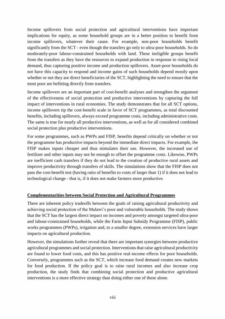
Income spillovers from social protection and agricultural interventions have important
implications for equity, as some household groups are in a better position to benefit from
income spillovers, whatever their cause. For example, non-poor households benefit
significantly from the SCT - even though the transfers go only to ultra-poor households. So do
moderately-poor labour-constrained households with land. These ineligible groups benefit
from the transfers as they have the resources to expand production in response to rising local
demand, thus capturing positive income and production spillovers. Asset-poor households do
not have this capacity to respond and income gains of such households depend mostly upon
whether or not they are direct beneficiaries of the SCT, highlighting the need to ensure that the
most poor are befitting directly from transfers.
Income spillovers are an important part of cost-benefit analyses and strengthen the argument
of the effectiveness of social protection and productive interventions by capturing the full
impact of interventions in rural economies. The study demonstrates that for all SCT options,
income spillovers tip the cost-benefit scale in favor of SCT programmes, as total discounted
benefits, including spillovers, always exceed programme costs, including administrative costs.
The same is true for nearly all productive interventions, as well as for all considered combined
social protection plus productive interventions.
For some programmes, such as PWPs and FISP, benefits depend critically on whether or not
the programme has productive impacts beyond the immediate direct impacts. For example, the
FISP makes inputs cheaper and thus stimulates their use. However, the increased use of
fertilizer and other inputs may not be enough to offset the programme costs. Likewise, PWPs
are inefficient cash transfers if they do not lead to the creation of productive rural assets and
improve productivity through transfers of skills. The simulations show that the FISP does not
pass the cost-benefit test (having ratio of benefits to costs of larger than 1) if it does not lead to
technological change - that is, if it does not make farmers more productive.
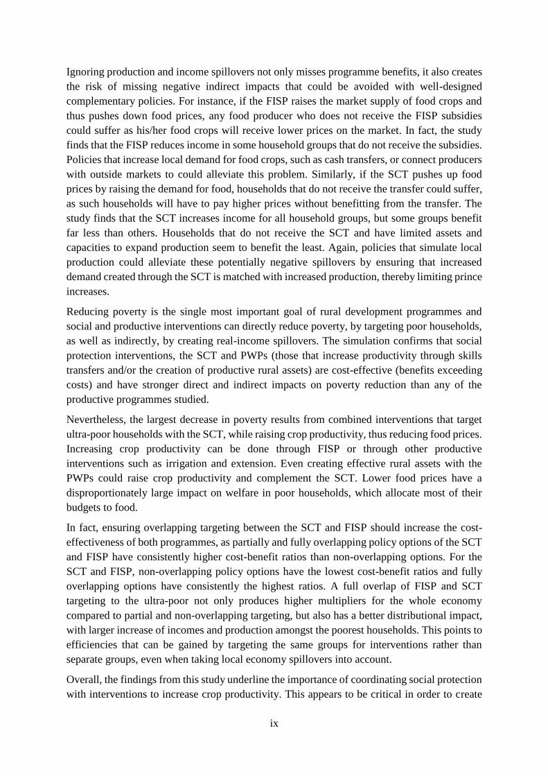
Complementarities between Social Protection and Agricultural Programmes
There are inherent policy tradeoffs between the goals of raising agricultural productivity and
achieving social protection of the Malawi’s poor and vulnerable households. The study shows
that the SCT has the largest direct impact on incomes and poverty amongst targeted ultra-poor
and labour-constrained households, while the Farm Input Subsidy Programme (FISP), public
works programmes (PWPs), irrigation and, to a smaller degree, extension services have larger
impacts on agricultural production.
However, the simulations further reveal that there are important synergies between productive
agricultural programmes and social protection. Interventions that raise agricultural productivity
are found to lower food costs, and this has positive real-income effects for poor households.
Conversely, programmes such as the SCT, which increase food demand creates new markets
for food production. If the policy goal is to raise rural incomes and also increase crop
production, the study finds that combining social protection and productive agricultural
interventions is a more effective strategy than doing either one of these alone.
ix
Ignoring production and income spillovers not only misses programme benefits, it also creates
the risk of missing negative indirect impacts that could be avoided with well-designed
complementary policies. For instance, if the FISP raises the market supply of food crops and
thus pushes down food prices, any food producer who does not receive the FISP subsidies
could suffer as his/her food crops will receive lower prices on the market. In fact, the study
finds that the FISP reduces income in some household groups that do not receive the subsidies.
Policies that increase local demand for food crops, such as cash transfers, or connect producers
with outside markets to could alleviate this problem. Similarly, if the SCT pushes up food
prices by raising the demand for food, households that do not receive the transfer could suffer,
as such households will have to pay higher prices without benefitting from the transfer. The
study finds that the SCT increases income for all household groups, but some groups benefit
far less than others. Households that do not receive the SCT and have limited assets and
capacities to expand production seem to benefit the least. Again, policies that simulate local
production could alleviate these potentially negative spillovers by ensuring that increased
demand created through the SCT is matched with increased production, thereby limiting prince
increases.
Reducing poverty is the single most important goal of rural development programmes and
social and productive interventions can directly reduce poverty, by targeting poor households,
as well as indirectly, by creating real-income spillovers. The simulation confirms that social
protection interventions, the SCT and PWPs (those that increase productivity through skills
transfers and/or the creation of productive rural assets) are cost-effective (benefits exceeding
costs) and have stronger direct and indirect impacts on poverty reduction than any of the
productive programmes studied.
Nevertheless, the largest decrease in poverty results from combined interventions that target
ultra-poor households with the SCT, while raising crop productivity, thus reducing food prices.
Increasing crop productivity can be done through FISP or through other productive
interventions such as irrigation and extension. Even creating effective rural assets with the
PWPs could raise crop productivity and complement the SCT. Lower food prices have a
disproportionately large impact on welfare in poor households, which allocate most of their
budgets to food.
In fact, ensuring overlapping targeting between the SCT and FISP should increase the cost-
effectiveness of both programmes, as partially and fully overlapping policy options of the SCT
and FISP have consistently higher cost-benefit ratios than non-overlapping options. For the
SCT and FISP, non-overlapping policy options have the lowest cost-benefit ratios and fully
overlapping options have consistently the highest ratios. A full overlap of FISP and SCT
targeting to the ultra-poor not only produces higher multipliers for the whole economy
compared to partial and non-overlapping targeting, but also has a better distributional impact,
with larger increase of incomes and production amongst the poorest households. This points to
efficiencies that can be gained by targeting the same groups for interventions rather than
separate groups, even when taking local economy spillovers into account.
Overall, the findings from this study underline the importance of coordinating social protection
with interventions to increase crop productivity. This appears to be critical in order to create

x
positive real-income multipliers and stimulate agricultural production while alleviating rural
poverty.
Social Cash Transfer Findings
The SCT creates significant multipliers and income gains for all household groups, with the
non-poor and moderately-poor benefitting the most from indirect spillovers. The simulation
models a range of options for the SCT with different transfer and coverage levels, from the
status quo of reaching ultra-poor and labour-constrained households to scenarios with broader
coverage and higher transfer levels. Under all design options the SCT creates large increases
in total rural income, substantially exceeding the amount transferred. These total real income
multipliers range from MK 1.88 to MK 1.91 and if measures are taken to avoid price increases
(e.g., productive interventions), these multipliers could rise to as high as 2.9 to 3.06 MK. While
SCT beneficiaries also benefit from spillovers, non-poor households are better placed to
capitalize on economic opportunities created by spillovers, as they have more resources to
increase their production of goods and services when local demand increases.
SCT income multipliers are similar across all options but the distribution of income gains
across household groups depends on who gets the transfers, with the poor benefitting mainly
from the direct transfer and the non-poor from the spillovers. The study finds that the non-poor
benefit the most from spillovers and that the ultra-poor and moderately-poor benefit only to a
limited degree from spillovers and rely primarily on the direct transfer for their income gains.
It is important to note that the study finds that the larger the transfer the greater the direct
impacts to the beneficiary groups and indirect spillovers. Finally, the SCT, despite being
targeted to poor and labour-constrained households, leads to increased production of crops,
livestock, retail, service and production goods amongst all household groups.
Public Works Programmes Findings
Income multipliers of PWPs are similar to those of SCT but rise considerably if PWPs can
increase productivity through asset creation and skills transfers. Total income multipliers of
PWPs are in the order of 2.9 MK. However, when land productivity is increased, additional
benefits per MK of transfer are created, resulting in multipliers of up-to 3.24 MK (assuming a
5% increase of land productivity). Similar to the SCT, the largest income gains are for the
targeted household groups. However income spillovers to non-beneficiary households,
including the non-poor, are also large and widespread. For every MK transferred, the incomes
of non-beneficiaries increase in real terms by between 0.8 and 1.9 MK. Real income multipliers
are larger for non-beneficiaries when PWPs increase productivity, as non-beneficiaries benefit
directly from higher productivity resulting from community assets. The largest percentage
impacts occur when PWPs target all poor households with labour with the highest number of
days and assuming productivity increases. Similar results are observed when targeting all ultra-
poor households with labour, strengthening the case for long-term PWPs with substantive
transfers and a investments in assets quality and skills transfers. Such investments are
important, as the magnitude of income and production effects depend on the quality of assets,

xi
skills transferred and their relevance to agricultural productivity. If productivity increases by
less than the 5% estimated in Ethiopia’s Productive Safety Net Programme (PSNP), total
income multipliers of PWPs will be at the lower bound of estimates given above.
Direct transfer and productivity effects of PWPs can potentially be are mutually reinforcing.
The biggest impact of productivity growth is to increase real income, because food prices fall
when productivity rises. PWPs, by increasing the productivity of crop production, mitigate
upward pressure on prices caused by the cash transfers. Price increases from increased demand
are offset by falling prices due to increased supply. This simulation demonstrates the
importance of creating effective PWP-assets (and transferring skills and knowledge) to increase
production and to mitigate price inflation caused by PWP-wages.
Farm Input Subsidy Programme Findings
Regardless of the scenarios studies, the FISP stimulates crop production and increases both
nominal and real incomes of targeted households. Crop output increases by 0.6% to 8.9% if
only the direct effects of the subsidies are considered. However, the study finds additional
effects of the FISP, beyond the subsidy, on crop productivity, suggesting that FISP
beneficiaries use different or improved technologies to produce crops. When considering the
full effect, including this element of technology change, crop output increases by 2% to 13.2%.
As with all interventions, real income impacts diverge from nominal impacts because of
changes in prices of local goods and services (including crop prices). All poor households with
land experience real income increase except under the options where the poorest household
groups are excluded from the FISP.
Directing the FISP toward households with land above the median significantly increases crop
production and rural incomes. Recently, directing the FISP towards households with land has
been piloted in some districts, which has been found to be enhance the FISP’s effectiveness.
This study appears to confirm these results. Simulating a policy option that keeps total coverage
and subsidy level constant but targets households with land above the median, the study finds
increases in overall crop production and rural income. Under these reforms, the impact of the
FISP without technology change rises from 15% to 8.5% (from 2.2% to 13.2%. with
technology change). Higher food production puts downward pressure on prices, increasing real
incomes for food consumers and leading to real income increases for all groups. Only ultra-
poor labour-constrained households with limited land have a slightly lower real income under
this reform, as they do not access the subsidy and receive lower prices for their crops. Total
real income increases from 1.67% to 3.34% without technology change and from 2.49% to
5.14% with technology change. It is important to note that households with land includes ultra-
poor and moderately poor households, and both groups show positive income and production
multipliers across all scenarios.
Targeting poor and ultra-poor farmers with access to land, rather than better off farmers,
produces larger income and production multipliers for the economy as a whole. The study
examines options for a more narrow coverage and cost of the FISP, comparing a more and less
pro-poor targeting approach, while maintaining the focus on productive farmers (land above

xii
1.5 acres), in line with current policy discussions. Remarkably, real income multipliers are
larger across the board when the FISP is targeted towards ultra-poor farmers and excludes the
non-poor. FISP increases crop production capacity of ultra-poor households with labour and
land by between 66% and 117%. However, when this group is excluded from the FISP their
production capacity falls between 50% and 55%. Interestingly, non-poor households with land
see income increase in real terms even when they do not directly receive the FISP, as they
benefit from lower prices and increase their production in other sectors (e.g. retail). From an
aggregate production perspective, targeting FISP to the most vulnerable (ultra-poor and
moderately poor) amongst “productive” farmers delivers a three times higher increase in the
total volume of crops produced in the economy, compared to when scenarios where the subsidy
is directed to better off-productive farmers.
It is important to note that the FISP has the potential to create negative spillovers, which are
especially concerning if the poor farmers with land are excluded from the programme. The
FISP’s income spillovers are large and positive under some scenarios but frequently they are
negative for households that do not receive FISP subsidies, due to the effect on food prices.
Subsidized inputs stimulate crop production and drive down prices, which negatively affects
surplus-producing farmers who do not receive the subsidy. In all scenarios non-beneficiaries
reduce crop production and when the poorest households are excluded from the programme,
their real income is negatively affected. In this case, the FISP causes a net welfare loss for the
poor and can have potentially regressive distributional effects.
Should the Government decide to reform the FISP, it should be directed to households with
land above the median, while those who no longer receive the FISP should be supported with
the SCT. This should create larger productive effects while limiting the adverse consequences
on the real incomes of former FISP beneficiaries. The resulting SCT targeted toward the poorer
households should have a greater impact on poverty. Still, careful attention should be paid to
the marginal farm household with low amounts of land who lose the FISP and may also be
impacted by the negative price effects from increased production by farmers with land above
1.5 acres that receive the FISP.
Irrigation and Extension Findings
Doubling the share of households with land above 1.5 acres and access to irrigation results in
a significant increase in crop production and total real incomes. Crop production increases by
9.55% (full cost annualized) and 15.58% (annual cost once operational), while incomes
increases by 5.87% and 11.3% respectively. It should be noted that nominal income effects of
the transfer and productivity increase even higher (6.09% and 14.66% respectively) but
increased irrigation is expected to drive down the price of crops, benefiting households with
irrigation but resulting in decreases of crop production for non-beneficiaries. Still, real incomes
rise across households because the cost of food consumption decreases with larger crop output
and spillovers benefit all households. Irrigation creates spillovers to other production sectors
as well. Not surprisingly, there are large income gains for household groups with land above
1.5 acres targeted by irrigation projects, however, spillovers on real income in households with
less land are also large. For the groups with land below 1.5 acres, those who receive the

xiii
spillovers but not the direct effects, the real income increases are smaller but still significant.
For ultra-poor groups, both those with direct access to irrigation and those who receive only
spillovers, real income gains range from 2.45% (limited labour and land) to 34% (labour and/or
land, under the annual cost once operational simulation). This simulation demonstrates the
potentially large and far-reaching impact of irrigation for the rural economy of Malawi.
Real income and production impacts of agricultural extension services are positive but smaller
than those of irrigation projects. Total real income rises by 2.48% and real incomes increase
for all household groups. Importantly, incomes rise by as much as 7% for ultra-poor
households. Access to extension services, like irrigation, creates real benefits that extend
beyond crop production, as there are small spillovers to other production sectors. Extension
has both real income and production multipliers that are above 2 MWK per MWK spent. Thus,
even though the percentage increases in real income and production due to extension is lower
than for irrigation, the benefit of 1 MWK spent on extension is more than for 1 MWK spent on
irrigation. Even if costs are born by households with land above 1.5 acres (as is the case with
those who receive extension services in this simulation), they still have positive income.
Extension services tend to benefit workers in rural areas (extension agents), who contribute to
the local economy by spending their wage on products and services from those locations.
Irrigation on the other hand has smaller multipliers and in fact a lower than one cost-benefit
ratio for both real income and production. The reason for this is the high capital cost for
imported irrigation equipment (either from outside Malawi or more generally outside the
simulated local economy). However, the multipliers do not capture the benefits of lower crop
prices that urban consumers receive due to irrigation improvements nor the resulting increase
in food security and exports. This may be significant given crop production increases of 16%
rising to 24% once completed. It should be noted that Malawi has seen a rise in smallholder
irrigation schemes, which may be a more cost-effective approach to expanding irrigation and
increase cost-benefit ratios.
1
1. Introduction
The objective of this report is to inform the design of agriculutural and social protection
interventions and associated resource allocation decisions, by simulating the cost-benefit of
alternative design options for standalone as well as different combinations of social protection
and agricultural programmes in Malawi. These analyses provide evidence on the policy options
to increase coordination and coherence between the two sectors with the objective of reducing
poverty, increasing incomes and enhancing agricultural production/productivity.
Social protection in Malawi is guided by the Malawi Growth and Development Strategy
(MGDS III) and the National Social Support Policy (NSSP). The Ministry of Finance,
Economic Planning and Development (MoFEPD) develops social protection policy coordinates
the implementation of social protection interventions by sectoral ministry and development
partners. The NSSP has four strategic objectives. These are: 1) To provide welfare support to
those unable to develop viable livelihoods; 2) To protect assets and improve the resilience of
poor and vulnerable households; 3) To increase productive capacity and the asset base of poor
and vulnerable households, and 4) To establish coherent synergies by ensuring strong linkages
to economic and social policies, and disaster management. The Malawi National Social Support
Programme (MNSSP) was designed to operationalize the NSSP over the period of 2012-2016,
based on the NSSP’s vision of enhanced quality of life for those suffering from poverty and
hunger and improved resilience of those vulnerable to shocks. To achieve these objectives, the
following five intervention areas where prioritized: 1) Social Cash Transfer (SCT), an
unconditional cash transfer targeted to ultra-poor and labour-constrained households; 2) Public
works programmes (PWPs) that provide regular payments to individuals in exchange for work,
with the objective of decreasing chronic or shock-induced poverty; 3) School meals
programmes (SMP) serve fortified corn-soya porridge to all children in targeted schools and
provide take-home-rations during the lean season; and 4) Village savings and loans, as well as
microfinance interventions, provide financial services including savings, loans and insurance
to rural Malawians.
In 2016, the MNSSP expired and after an extensive process of stakeholder consultations, a
successor programme, the MNSSP II was developed and finalized. The MNSSP II will run for
five years and will build on the successes and lessons learned during the implementation of the
first MNSSP. It maintains the same prioritized interventions but these are organised around
thematic priority areas, thus providing enhanced strategic policy guidance on promoting
linkages, strengthening systems, and improving monitoring activities.
Similarly, the National Agricultural Investment Plan (NAIP) is the framework for coordinating
and prioritising investments in agriculture by government agencies, development partners and
Non-State Actors including the private sector. The NAIP adopts the goal of the National
Agricultural Policy and has three objectives: (1) broad-based and resilient agricultural growth;
(2) improved well-being and livelihoods of Malawians; and (3) improved food and nutrition

2
security. Speaking especially to points (3) and (4) of the MNSSP and to points (2) and (3) of
the NAIP, this analysis brings together the priorities of the MNSPP and of the NAIP.
The agricultural policy and programmes in Malawi, coordinated and implemented by
MoAIWD, consist of programmes to increase yields for staple crops (predominately maize),
support extension services, research and disseminate new varieties, aid in animal husbandry,
support commercialization and agricultural import/export markets, promote food security, and
aid poor and vulnerable small farmers. In the recent past the Farm Input Subsidy Programme
(FISP) has been– in budgetary terms – the largest programme, providing input sudsidies for
fertilizer, better maize seed varieties and other farm inputs.1 This programme was intended to
increase yields and aid poor farmers. Other important programmes include irrigation and
extension services for small and large farmers as well as the development of watershed
resources.
The programmes considered in this report include a subset of activities from the social
protection and agricultural programmes: the SCT and Local Development Fund (LDF) PWP
on the social protection side; and the FISP, extension services, and irrigation services on the
agriculture side. These interventions are considered priority interventions for study by the
different stakeholders of this analysis: the Government of Malawi (GoM), the International
Labour Organization (ILO), the United Nations Food and Agriculture Organization (FAO), and
the United Nations Children’s Fund (UNICEF). They are also significant programmes – in
terms of their budget and coverage.
Using a local economy wide model, this study aims at simulating ex-ante the impacts on the
targeted beneficiaries of social protection and agriculture programmes, as well as the spillover
effects on other households in the local (rural) economy. It proposes to address the following
policy questions: What could be the most effective policy scenario(s), in terms of: a) supporting
the poorest households; b) increasing agricultural production; c) stimulating economic growth
and d) reducing poverty and inequality. The report also includes cost-benefit analysis (CBA)
of policy options discussed above to compare their relative effectiveness and combinations of
these options in order to evaluate potential synergies. It is expected that the results and
recommendations of this analysis will aid in the formulation and implementation of the 2018-
2022 NAIP, the follow-up to the Malawi Agricultural Sector Wide Approach (ASWAp), and
new Malawi National Social Support Programme (MNSSP II) launched in 2018.
1 According to the ASWAp Review Final Draft for 2010-2014 (2016), a total of 1 billion USD or 72% of this
period’s government expenditure on agriculture was on FISP. Agriculture makes up approximately 30% of GDP
for Malawi.
3
2. Methodologies
All of the programmes outlined above - the SCT, PWPs, FISP, irrigation and extension services
- have direct impacts on the beneficiary households: those households directly benefiting from
a policy. They also potentially have benefits beyond the beneficiary group: other households
that are in the same village or nearby villages of the beneficiary households but do not receive
direct benefits of a programme.
2.1. Impacts of programmes on beneficiary households
The impacts of interventions on targeted households can be estimated using experimental
methods if the programme treatment is random, or with quasi-experimental methods if they are
non-random but a comparison group can be created synthetically using matching methods.
Rigorous randomized control trials (RCTs) are not available to evaluate the direct impacts of
FISP, extension, irrigation investments, or other productive interventions on the households
that are directly “treated” by these interventions.2 Using a large sample of micro-data from
household surveys, we can estimate a model to predict crop yield for households that currently
do and do not receive FISP subsidies, extension services, and access to irrigation. Under general
conditions, this gives us the best linear unbiased predictor of crop yield, conditional upon
whether (or to what extent) households are treated by the interventions, regardless of whether
or not the interventions randomly target the rural population. This may not tell us whether
changing the interventions—their targeting or magnitude—will cause changes in crop yield if
the targeting is not random.3
For simpler simulations, for example, of changes in crop output prices, a structural approach
can be used. We can use micro data together with econometric methods to estimate agricultural
household models for different household groups. The agricultural household models can then
be used to simulate the direct impacts of programmes or combinations of programmes on the
targeted groups, similar to what is done in Singh, Squire and Strauss’ (1986) classic book. For
example, the FISP lowers the price of an input, which stimulates the demand for the input and
also creates an income effect in the FISP beneficiary households.4 Once we have estimated an
agricultural household model, the challenge is to determine how to actually simulate different
interventions or combinations of interventions. For some interventions, like input subsidies,
productivity increases, or output price supports, simulating the intervention in the model is
fairly straightforward. For others, for example, programmes that loosen liquidity constraints on
production (as cash transfers might do), it is somewhat more challenging and may require
2 Experimental evaluation results exist for SCT (e.g. Asfaw et al. 2016 and UNC, 2016) and PWP (e.g. Beegle,
Galasso, and Goldberg, 2017) but they are not representative of nationally scaled up programmes. There are also
quasi-experimental evaluations of FISP including two on synergies between the FISP and SCT (Daidone et al.
2017 and Pace et al. 2017). We add to these latter studies by including cost-benefit analysis and additional
programmes (PWP, irrigation, and extension services). 3 An econometric approach that controls for crop inputs, household characteristics and district fixed effects to
estimate direct impacts of FISP, irrigation, and extension on predicted crop yields is used. This is a reasonable and
conservative approach to evaluate the impacts of these three interventions, which may affect crop production in
complex ways—including changes in the ways in which farmers grow crops. 4 These impacts come out of the first-order conditions for optimization in the agricultural household model.

4
additional information from studies that have tested for programme impacts on beneficiary
households. Fortunately, there is a rich literature on the direct impacts of many of these
programmes on beneficiary households that we can draw from as needed.
2.2. Local Economy-wide Impact Evaluation (LEWIE)
Existing research shows that significant income gains in rural areas can extend beyond the
direct beneficiary households, as a result of consumption and other local linkages (e.g., Thome,
Filipski, et al. 2013; Kagin, et al. 2014; Taylor and Filipski 2014). Given the income gained by
these vulnerable households, and its multiplier effects in local economies, the result could be
substantial benefits for ineligible households living in the local economy, as well. It is quite
possible that the impacts of these programmes on communities as a whole are larger than the
direct impact originating from cash or in-kind transfers received by the beneficiaries,
themselves.
In real life, beneficiaries interact with other households within local economies. Market
linkages transmit the impacts of programmes from the directly affected households to others in
the local economy. We designed and carried out a Local Economy-Wide Impact Evaluation
(LEWIE) to simulate the direct and indirect impacts of alternative policy options. The LEWIE
model captures multiplier effects of government programmes on the activities and incomes of
target groups as well as the indirect impacts on groups not targeted by these programmes.5 The
households that are not eligible for, or not targeted by, programmes, with few exceptions, are
beyond the purview of experimental approaches. By treating eligible households with cash
transfers and other interventions, social protection and agriculture programmes “treat” the local
economies of which these households are part. Market interactions shift impacts from
beneficiary to non-beneficiary households. For example, beneficiaries of the SCT spend a large
part of their cash on goods or services supplied by local farms and businesses. As local
production expands to meet the new demand, incomes in the households connected with these
farms and businesses rise, together with the demand for labour and other inputs. This generates
additional rounds of spending and income growth in the local economy. As impacts swirl
through the local economy, the programme is likely to benefit non-beneficiaries, including local
business owners, traders, farmers, livestock producers, and others. However, if the local supply
of goods and services is not responsive or elastic, there may also be inflationary pressures that
create costs for local consumers and cause real income gains to diverge from nominal ones.
Table 1 presents a theory of change table which describes the channels in which final impacts
occur. Figure 1 summarizes the LEWIE model and how channels through which different
policies could have impacts on beneficiary and non-beneficiary households in the rural
economy.
5 Some examples of these types of studies are in included in the PtoP project of the UNFAO,
http://www.fao.org/economic/ptop/publications/reports/en/

5
It is important to note that spillovers accrue to non-beneficiaries as well as to beneficiaries,
which add to the direct effects on beneficiaries. Direct and spillover effects on beneficiaries are
estimated simultaneously in the LEWIE model, and are part of the local economy-wide effects.
The model developed for this study builds upon the previous use of LEWIE in Malawi to study
the impacts of cash transfers by Taylor and Filipski (2014, Chapter 10).6 This study represents
the first comprehensive rural economy cost-benefit analysis of social protection and agricultural
production programmes in Malawi.
The LEWIE model includes a breakdown of household groups with respect to their eligibility
for each of the programmes. Each simulation reports the distributional impacts of the policies
across different household groups as well as the overall impacts on the rural economy. This
study defines the local economy as all of rural Malawi. An additional benefit of using a LEWIE
approach is that we can simulate impacts on beneficiaries and non-beneficiaries of different
programme design options as well as combinations of programmes.
6 The LEWIE methodology has been thoroughly vetted through the publication of a major Oxford University
Press book (Taylor and Filipski 2014), several articles in academic journals, and most recently a study on host-
country impacts of refugees and refugee assistance in Rwanda (Taylor, Filipski et al. 2016). For more on the
LEWIE methodology see Appendix B.

6
Table 1. Theory of Change - Summary of Programme Impacts on Beneficiary and Non-
Beneficiary Households
7 Throughout the report, technology change with respect to FISP refers to increases in yields that are independent
of input use. FISP stimulates input demands. We find evidence (see below) that FISP is also associated with higher
yields even at the same levels of input usage. This reflects increases in farmer efficiency, beyond the FISP’s direct
subsidy effect.
Programme Channel of impact on
beneficiaries
Spillovers to non-
beneficiaries
Rural economy
impact
SCT:
• Cash transfer to
ultra-poor
household groups
Increase in exogenous income Spending on goods from
local farms and
businesses
Increased
employment
Increased
incomes
Reduced poverty
Increased
production
Economic growth
Possible inflation
(Potentially
lower production
and/or income in
non-beneficiary
households due
to lower crop
prices, reduction
in hired labour)
Production expands to
meet increased demand
If production does not
expand, inflationary
impacts occur
PWPs:
• Wages paid to
labour
unconstrained
households for
constructing
public works
• Assets created
• Skills and
technology
transferred
Increase in exogenous income Spending on local farms
and businesses
Public works such as watershed
management and irrigation
canals increase productivity of
land for all households in rural
Malawi. Transfer of skills and
technology through public works
can improve productivity of
direct beneficiaries.
Extra income from
crop production is
spent in the local
economy leading to
increases in local
production
Increase in hiring of
agricultural labour
Price changes due to
beneficiary
households’ changes
in production
increase or decrease
non-beneficiary
household
production across
activities.
FISP:
• Fertilizer coupons
distributed to low
income maize
farmers
Farm households purchase
additional fertilizer and seeds
Farm households experience
technology change, increasing
yields through increased
efficiency due to the FISP7.
Irrigation
• Irrigation systems
built for HHs with
land above 1.5
acres
Land productivity for crops
increases for beneficiary
households
Extension
• Government
extension services
provided to HHs
with land above
1.5 acres
New information leads to higher
yields for beneficiary households
7
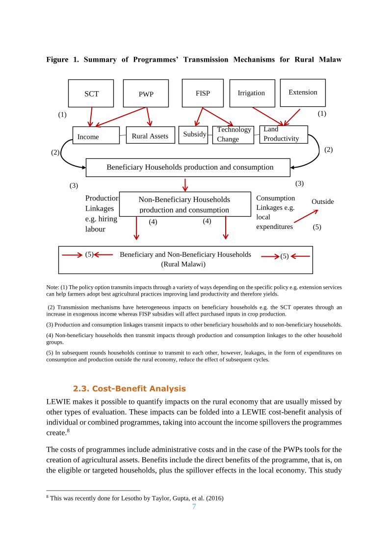
Figure 1. Summary of Programmes’ Transmission Mechanisms for Rural Malaw
Note: (1) The policy option transmits impacts through a variety of ways depending on the specific policy e.g. extension services
can help farmers adopt best agricultural practices improving land productivity and therefore yields.
(2) Transmission mechanisms have heterogeneous impacts on beneficiary households e.g. the SCT operates through an
increase in exogenous income whereas FISP subsidies will affect purchased inputs in crop production.
(3) Production and consumption linkages transmit impacts to other beneficiary households and to non-beneficiary households.
(4) Non-beneficiary households then transmit impacts through production and consumption linkages to the other household
groups.
(5) In subsequent rounds households continue to transmit to each other, however, leakages, in the form of expenditures on
consumption and production outside the rural economy, reduce the effect of subsequent cycles.
2.3. Cost-Benefit Analysis
LEWIE makes it possible to quantify impacts on the rural economy that are usually missed by
other types of evaluation. These impacts can be folded into a LEWIE cost-benefit analysis of
individual or combined programmes, taking into account the income spillovers the programmes
create.8
The costs of programmes include administrative costs and in the case of the PWPs tools for the
creation of agricultural assets. Benefits include the direct benefits of the programme, that is, on
the eligible or targeted households, plus the spillover effects in the local economy. This study
8 This was recently done for Lesotho by Taylor, Gupta, et al. (2016)
(4) (4)
Land
Productivity
Beneficiary Households production and consumption
Technology
Change
(5)
(5)
(2)
(1)
SCT PWP FISP Irrigation
Production
Linkages
e.g. hiring
labour
Consumption
Linkages e.g.
local
expenditures
Income
Non-Beneficiary Households
production and consumption
Beneficiary and Non-Beneficiary Households
(Rural Malawi) Non
(1)
(2)
(3)
Outside
(5)
Extension
Rural Assets Subsidy
(3)

8
focuses on economic benefits. Other possible benefits include the accumulation of productive
capital, social capital, improved nutrition, and education. We have estimated some of these
additional impacts using experimental or quasi-experimental methods for social cash transfers
elsewhere (e.g., see Taylor and Kagin 2016; Taylor, Gupta and Davis 2016); however, the lack
of impact evaluation results in these social dimensions for each of the programmes considered
in the current exercise prevents us considering them in this analysis.9 In the absence of a proper
baseline and follow-up survey for each of the policy scenarios we consider below makes this
approach unfeasible in Malawi. LEWIE offers a particularly attractive alternative in cases
where experimental or quasi-experimental information on beneficiaries and non-beneficiaries
is not available.
3. Data
We primarily use the Integrated Household Survey III (IHS3) to build the LEWIE model for
rural Malawi. The survey data encompass economic activities, demographics, welfare and other
information on households and cover a wide range of topics, including the dynamics of poverty
(consumption, cash and non-cash income; savings; assets; food security; health and education;
vulnerability and social protection). Although the IHS3 household questionnaire covers a wide
variety of topics in detail, it intentionally excludes in-depth information on topics covered by
other surveys that are part of the NSO’s statistical plan (for example, maternal and child health
issues covered at length in the Malawi Demographic and Health Survey). For agriculture, the
data cover crop production and inputs during the dry and rainy agricultural season in 2009-
2010 as well as livestock production and inputs.10 They also include questions pertaining to
PWPs, the SCT and FISP by season.
Construction of the LEWIE model requires data on intermediate input demands by retail,
service, and local non-agricultural production sectors, as well as value added shares for each
business type. This includes data on products and services purchased by businesses in the local
economy and how much value added these purchases add to the final products sold. Although
this information was not asked in the IHS3, it was gathered as part of the SCT impact study by
Thome et al. (2015). The limitations of these data, besides being from a source other than the
IHS3, are that they are not representative of all rural districts in Malawi, but only a small subset
of districts. Nevertheless, there is good reason to believe that input-output relationships in retail,
service, and other non-agricultural production activities do not vary widely across rural areas
of Malawi; for example, a village store is a village store, wherever it is. A detailed table of
weighted averages of key variables used in our analysis appears in Appendix B.
9 Social dimensions could be estimated for the Social Cash Transfer Programme (since the experimental data are
available), but then the results would not be comparable with scenarios that involve other interventions such as
PWP and FISP. 10 Unfortunately, at the time of this report the IHS4 is currently in the field so data from the more recent 2015-
2016 crop season cannot be utilized.

9
4. Programmes considered
The following agricultural and social protection programmes are included in the policy
simulations presented below:
4.1. The Social Cash Transfer
The SCT is an unconditional transfer targeted to ultra-poor and labour-constrained households.
It is operated by the Ministry of Gender, Children, Disability and Social Welfare (MoGCDSW).
Ultra-poor households are statistically defined as having a total annual consumption lower than
the food poverty line of 22,007 MK and the SCT operationalizes this through community
targeting and criteria such as eating less than one meal a day. Labour constrained households
are defined based on the ratio of members that are ‘not fit to work’ to those ‘fit to work’. ‘Unfit’
in this context means being outside of the economically active ages (below 18 or above 64),
having a chronic illness or disability or being otherwise unable to work. A household is
considered labour constrained if it has no members that are ‘fit to work’ or if the ratio of ‘unfit’
to ‘fit’ exceeds three (Abdoulayi et al, 2014).
For the programme year 2016/2017, the SCT reaches all 28 districts of Malawi to approximately
330,000 households. This is approximately 12 percent of rural households. The main objectives
of the SCT are to reduce poverty and hunger and increase school enrollment. Transfer amounts
vary by household size and number of children enrolled in school. In 2016/2017, the transfer
level varied between MK 1,700 and MK 3,700 per month, depending on household size, with
a bonus of MK 500 per month for each child enrolled in primary school and MK 1000 for each
child in secondary school.
4.2. Public works programmes
The LDF financed PWP provides a conditional cash transfer targeted to poor households with
labour capacity. It is implemented by Malawi’s 28 District Councils and the Ministry of Local
Government and Rural Development (MoLGRD). Beneficiary selection is done via self-
selection. The programme covers the whole country and reaches 450,000 households in
2016/17 for 3 years (same beneficiaries). In 2017, the transfer amount per beneficiary was MK
600 per day for 48 days per year, around MK 28,800 per year. The main objectives of the PWP
is to increase incomes and food security of poor rural households and to create productive
community assets. Historically, these community assets have been roads and bridges but the
current focus lies on watershed management projects.
4.3. The Farm Input Subsidy Programme
In 2005/06 the Government introduced the FISP against the background of unfavorable weather
conditions impacting agricultural production, prolonged and widespread food shortages and
high input prices in the absence of appropriate farm input loans for smallholder farmers. The
primary purpose of the programme was to increase resource-poor smallholder farmers’ access
to improved agricultural inputs in order to achieve food self-sufficiency and increase farm
households’ income through increased food and cash crop production. The FISP operates
nationwide and covers around 50% of Malawi’s smallholder farmers (1.5 million households).

10
Transfers amount to two vouchers allowing the purchase of 100 kg of fertilizer and 5-8 kg of
seeds at heavily discounted prices. The transfer value was MK 29,400 per household/per year
in the 2015/16 growing season.
In the 2016/2017 farming season the FISP has undergone substantive reforms. Government
deficits and programme cost overruns have made the budget for FISP untenable for the
Government, which has led to a substantive reduction in the scale of the programme, amongst
other reforms. For the 2016/17 farming season, 900,000 farmers have received coupons,
compared to 1.5 million in previous years (Logistics Unit, GoM 2017). These farmers are being
chosen from a pool of 4.2 million maize farmers who did not receive the subsidy in the 2015/16
season. Other reforms include distributing the subsidized inputs through primarily private
agricultural input suppliers, giving a fixed amount of subsidy, MK 15,000 per beneficiary, and
allowing the market to determine the actual price of maize seeds and fertilizer. For the 2017/18
season, the FISP is to focus not on resource-constrained smallholder farmers but on those who
have productive capabilities, that is, those that cultivate two or more acres of land.
Correspondingly, this study regards households with land above the median (1.5 acres) as those
with more productive capacity.
Despite the proposed reform for the 2016/17 farming season, alternative policy options
regarding FISP targeting and implementation are still under discussion.11 These policy options
envisage the targeting of poor and less poor agricultural households in different proportions,
ranging from the exclusive targeting of smallholder farmers at the bottom of the poverty and
wellbeing distribution to the exclusive targeting of farmers that have productive capabilities,
including sufficient land and labour, and are more commercially-oriented.
4.4. Extension services
The state of agricultural extension services in Malawi is considered very weak but Malawian
experts suggest that strengthened extension services could potentially have sizable impacts on
agricultural productivity. There are approximately 15 extension workers per planning area. In
the Lilongwe district there are 19 planning areas, so approximately 285 workers. If there are
approximately 1 million people in this district, and according to IHS3 47% engage in
agriculture, there is only one extension worker for every 1,650 farmers. According to IHS3
data, only 23% of households report having had a government extension worker give them
advice during the previous rainy season (2008-2009). According to a representative from the
MoAIWD, visits with an extension officer can help improve yields 60%-80%. Data from the
IHS3 has been sued to estimate the effect of extension services on targeted farmers in Malawi.
4.5. Irrigation projects
The Government desires to invest considerably in scaling-up irrigation but currently does not
devote significant resources to this policy. According to the IHS3 data, 17% of agricultural
households reported having access to irrigation. The Department of Irrigation (DOI) stated that
11 Authors’ discussions with a representative from the Ministry of Agriculture, Irrigation and Water Development.

11
approximately 104,000 hectares of land were irrigated as of 2014/15. FAOSTAT, FAO’s
statistical databases, states that of the agricultural land in the country, only 1.3% is irrigated
(2011). Several irrigation plans were implemented as part of the ASWAp plan 2011-2015. One
of the plan’s main aim was to increase sustainable irrigation to 280,000 hector or 4% of total
agricultural land. A partner in this aim has been the Rural Livelihood and Agricultural
Development Project (IRLAD), a joint project by the World Bank, IFAD and the Government.
Agricultural intensification through irrigation has the potential to quadruple yields and provide
at least two harvests per hectare to small farmers in a given year. A number of studies show
that farmers involved in irrigation schemes in Malawi were more food self-sufficient and
economically better off than farmers in rain-fed agriculture. At the time of design of the IRLAD
project, the total formal or semi-formal irrigated area in Malawi was about 28,000 hectares
(compared with a potential of up to 0.5 million hectares), of which 6,500 hectare were under
self-help small holder schemes (farms with less than 10 hectares), 3,200 hectare were under
Government-run smallholder schemes, and 18,300 hectare were in estates (farms with 10-500
hectares).
5. Household groups
The LEWIE analysis requires a practical household taxonomy in order to carry out simulations
and compare outcomes across beneficiary and non-beneficiary household groups.
All households in rural Malawi were organized into the following categories, as shown in Table
2: Category I (non-poor), II (moderately poor labour unconstrained), III (moderately poor
labour constrained), IV (ultra-poor labour unconstrained), and V (ultra-poor labour
constrained). Each of these, in turn, was split into two sub-categories to take into account land
possession. The non-poor households (I) are split into those with land above the median (~1.5
acres or ~0.6 hectares) (A) and land below the median (B). The moderately poor were split into
four groups: Labour unconstrained (C) and labour constrained (D) with land above the median,
and labour unconstrained and constrained with land below the median (E and F, respectively).
The ultra-poor group was similarly disaggregated into labour unconstrained with land above
the median (G) and below the median (H), and labour constrained with land above the median
(I) and with land below the median (J). A cutoff of 1.5 acres was used to distinguish land-
constrained from land-unconstrained households. Based on the IHS3 data on production and
landholding size, we judged that dividing households by median landholding size was a
reasonable criterion for determining land constraints.
In all, there are ten household groups in the LEWIE model. The underlying assumption behind
this household taxonomy is that both poverty, labour availability and access to land are key
factors influencing programme impacts. This is an important nuance, especially for the LEWIE
analysis on combined interventions.

12
Table 2. Household Taxonomy
Land above 1.5 acres Land below 1.5 acres
Non poor I A B
Moderately
poor
Labour Unconstrained II C E
Labour Constrained III D F
Ultra poor
Labour Unconstrained IV G H
Labour Constrained V I J
Descriptive statistics generated from IHS3 data across a variety of variables for each household
group are given in Appendix B. A subset of these statistics are given below in Table 3.12 As
expected, labour constrained households have higher dependency ratios and shares of ill and/or
disabled members. However, it is important to note that land size more accurately reflects
average expenditures; the poor household groups (non-poor, moderately poor and ultra-poor)
that cultivate less land have lower average expenditures, but within poverty groups labour
constrained households are not necessarily poorer than those with labour.13
Table 3. Descriptive Statistics across Household Groups
12 Although income is reported as well as expenditures, consistent with other literature in Malawi (e.g.
Meerendonk, Cunha, and Juergens, 2015), and believing it more accurately reflects actual income, we use yearly
total expenditure as our baseline income for analysis. 13 Across all households, households that are labour constrained have lower expenditures and income than labour
unconstrained households.
A B C D E F G H I J
Non-poor HH
with land >=
1.5 acres
Non-poor HH
with land < 1.5
acres
Moderately poor HH
with unconstrained
labour and land >=
1.5 acres
Moderately poor HH
with constrained
labour and land >= 1.5
acres
Moderately poor
HH with
unconstrained
labour and land <
1.5 acres
Moderately poor HH
with constrained
labour and land <
1.5 acres
Ultrapoor HH with
unconstrained
labour and land >=
1.5 acres
Ultrapoor HH
with
unconstrained
labour and land
< 1.5 acres
Ultrapoor HH with
constrained
labour and land
>= 1.5 acres
Ultrapoor HH
with
constrained
labour and
land < 1.5
acres
Socio-demographics
HH size 4.28 3.33 4.87 6.04 4.04 4.83 5.42 4.68 6.70 5.56
Percent of total rural households 17% 30% 4% 3% 8% 9% 6% 11% 5% 7%
Percent of HH where the head attended school 25% 31% 19% 16% 20% 15% 11% 16% 7% 12%
Percent of HH that are female headed 23% 30% 12% 30% 18% 49% 14% 18% 30% 50%
Percent of HH where the head is unfit SHWR
and/or chronically ill 10% 12% 3% 21% 3% 28% 2% 2% 14% 18%
Dependency ratio 2.62 2.36 2.29 4.17 2.19 4.00 2.43 2.38 4.37 4.23
Crops
Total value of crop harvest 142,725 68,618 136,109 139,210 61,779 62,096 95,129 47,521 97,174 49,396
Yields (output value per acre) 57,859 76,644 55,262 53,849 69,377 68,890 40,695 54,663 40,849 57,578
Land cultivated in acres 2.50 0.93 2.50 2.63 0.92 0.97 2.40 0.94 2.44 0.94
Livestock
Value of livestock owned now and livestock
byproducts from last 12 months 267,216 45,530 93,609 26,312 210,068 75,429 61,837 15,471 98,410 22,540
Household Enterprise
HH annual own business sales 176,946 329,225 66,197 41,427 59,407 65,659 25,109 27,495 35,788 25,781
HH annual own business profits 65,493 151,708 28,217 18,226 24,174 28,632 11,556 11,381 20,972 13,207
Expenditures
HH annual expenditures on food 787,094 658,818 352,185 433,464 293,401 350,364 211,723 180,881 249,983 205,462
HH annual expenditures 1,029,945 857,447 434,014 534,353 356,207 430,831 249,805 215,415 300,283 245,691
Income
HH annual income 962,455 1,194,584 627,862 670,878 492,604 482,230 512,174 343,268 466,474 351,133
Notes: All values are in 2016 MK yearly averages by household group

13
6. Construction of the LEWIE model
Data from the IHS3 were used to construct the LEWIE model. Specifically, we used
econometric regressions to estimate production functions for each sector (crops, livestock,
retail, services, non-farm production) and expenditure functions for each good and household
group (see Tables 3 and 4). The survey data were also used to obtain starting values of all
variables in the model: inputs and output by production sector and incomes and expenditures
by good for each household group. Combining the production and expenditure equations gives
us an agricultural household model for each of the ten household groups. Market-clearing
conditions link these households together into a LEWIE model for rural Malawi, which we used
to simulate the rural economy-wide impacts of alternative individual and combined
interventions.
6.1. Modelling household production
Table 4 reports the econometric estimates of production parameters by sector and household
group. Production functions embody the technologies used to turn family and hired labour,
land, capital, and purchased inputs like fertilizer into outputs for each production activity.
Overall, households in rural Malawi use similar technologies to produce a given type of good.
For example, there are no major differences in labour or merchandise purchases per MK of
sales in rural stores. However, there are some differences in technologies for crop production
between poor and non-poor households. Table 4 presents crop parameter estimates for each of
these two broad groups of households.14
Ultra-poor household crop production is intensive in labour but not in capital or purchased
inputs. The estimated parameters are the shares of factors in value added. (They also represent
the elasticity of output with respect to each factor.) Labour accounts for 47% of crop value-
added in non-poor and moderately poor households, but 85% in ultra-poor households. In non-
poor and relatively poor households, purchased inputs account for just over 11% of crop value-
added, compared with 8.3% in ultra-poor households. Capital (machinery and tools) accounts
for 11% of value-added in non-poor and moderately-poor households but only 1% in ultra-poor
households.
Livestock production is much less labour intensive than crop production, and it is much more
intensive in land and capital (including investment in herds). Retail is intensive in capital
(including investments in inventory), though less so in ultra-poor household retail businesses.
14 For each production function we regressed the log of the output on the factor inputs, with dummy variables
controlling for different household groups and interaction terms of the household groups with the factor inputs.
Standard errors are not reported for some factors whose value-added shares were calculated as residuals assuming
constant returns to scale. For inputs that may have zero values, following the World Bank study on poverty in
Malawi (Forthcoming) and D’Souza and Jolliffe (2014) we use the inverse hyperbolic sine transformation (IHST)
instead of the log transformation. IHST is a logarithmic-like transformation that enables negative as well as zero-
valued observations and enables the coefficients to be interpreted as elasticities.
14
Services and non-farm production are more labour -intensive than retail or livestock production
but less so than crops.
These estimates are consistent with what one would expect and also with production parameters
in other LEWIE models for sub-Saharan Africa. They highlight that changes in production
create important labour market linkages, particularly in crop, service, and non-agricultural
production activities. Changes in the supply and demand for retail goods have smaller, but still
important, employment effects: Labour accounts for just over a quarter of value-added in rural
stores.
As sectors increase production they purchase inputs inside or outside the local economy.
Purchases inside the local economy create local income linkages that contribute to the multiplier
effects of production increases. Purchases outside the local economy transmit impacts to urban
areas inside Malawi or to the rest of the world. A useful index of local versus outside input
linkages is the ratio of MK outlays on inputs to total value-added in each sector. The figures
below use data on locations from the SCT impact evaluation of Thome et al. (2015). Figure 2
shows these ratios for input purchases outside the rural economy by all five sectors. Figure 3
shows the same but for inputs purchased inside the rural economy. Detailed data appear in
Appendix B.

15
Table 4. Estimated Production Parameters, by Household Group
Note: HL is hired labour, FL is family labour, K is capital, PURCH is purchased inputs, and C-D is Cobb Douglas.
Many of the interaction terms in the pooled regressions used to determine differences in production function
parameters across household groups were insignificant. Thus, there are similarities across household groups for
parameter estimates. This is not surprising given that one would not expect technology to change too much for
similar households in a given activity. This may also be due to insufficient data to determine differences.
Non-poor Moderately Poor Ultrapoor
Unconstrain
ed &
Constrained
Labor
Unconstrained &
Constrained
Labour
Unconstrained &
Constrained
Labor
All Land Sizes All Land Sizes All Land Sizes
A, B C,D,E, F G, H, I, J
HL 0.116 0.116 0.297
FL 0.358 0.358 0.559
LAND 0.300 0.300 0.073
K 0.113 0.113 0.010
PURCH 0.114 0.114 0.083
HL 0.015 0.015 0.030
FL 0.030 0.030 0.056
LAND 0.036 0.036 0.092
K 0.013 0.013 0.013
PURCH 0.009 0.009 0.011
C-D Shift Parameter 6.778 6.686 5.636
Standard Error 0.151 0.154 0.271
HL 0.132 0.132 0.132
FL 0.102 0.102 0.102
LAND 0.434 0.434 0.434
K 0.278 0.278 0.258
PURCH 0.055 0.055 0.099
HL 0.032 0.032 0.032
FL
LAND 0.032 0.032 0.032
K 0.004 0.004 0.010
PURCH 0.019 0.019 0.017
C-D Shift Parameter 6.965 6.965 6.965
Standard Error 0.094 0.094 0.094
HL 0.107 0.107 0.107
FL 0.158 0.158 0.158
K 0.736 0.477 0.477
HL 0.040 0.040 0.040
FL 0.038 0.038 0.038
K
C-D Shift Parameter 5.737 8.330 8.330
Standard Error 0.577 0.323 0.323
HL 0.222 0.222 0.222
FL 0.149 0.149 0.149
K 0.629 0.629 0.629
HL 0.053 0.048 0.048
FL 0.080 0.045 0.045
K
C-D Shift Parameter 9.919 9.919 9.919
Standard Error 0.024 0.024 0.024
HL 0.183 0.183 0.183
FL 0.294 0.294 0.294
K 0.523 0.472 0.472
HL 0.045 0.045 0.045
FL 0.048 0.048 0.048
K
C-D Shift Parameter 7.953 7.953 7.953
Standard Error 0.358 0.358 0.358
Estimated Parameters
Standard Errors
Services
Estimated Parameters
Standard Errors
Non-farm Production
Retail
Estimated Parameters
Standard Errors
Standard Errors
Livestock
Estimated Parameters
Standard Errors
Crops
Estimated Parameters
Sector/Factor
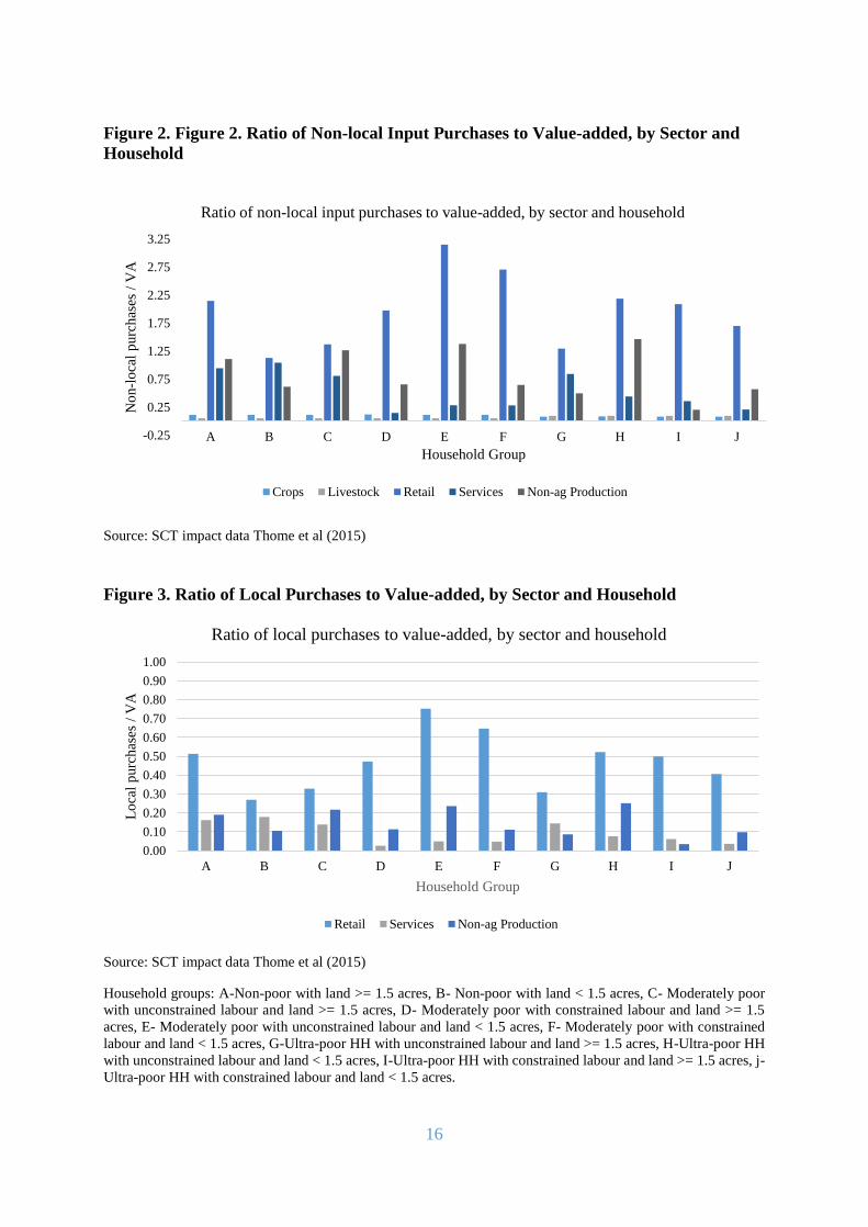
16
Figure 2. Figure 2. Ratio of Non-local Input Purchases to Value-added, by Sector and
Household
Source: SCT impact data Thome et al (2015)
Figure 3. Ratio of Local Purchases to Value-added, by Sector and Household
Source: SCT impact data Thome et al (2015)
Household groups: A-Non-poor with land >= 1.5 acres, B- Non-poor with land < 1.5 acres, C- Moderately poor
with unconstrained labour and land >= 1.5 acres, D- Moderately poor with constrained labour and land >= 1.5
acres, E- Moderately poor with unconstrained labour and land < 1.5 acres, F- Moderately poor with constrained
labour and land < 1.5 acres, G-Ultra-poor HH with unconstrained labour and land >= 1.5 acres, H-Ultra-poor HH
with unconstrained labour and land < 1.5 acres, I-Ultra-poor HH with constrained labour and land >= 1.5 acres, j-
Ultra-poor HH with constrained labour and land < 1.5 acres.
-0.25
0.25
0.75
1.25
1.75
2.25
2.75
3.25
A B C D E F G H I J
No
n-l
oca
l p
urc
has
es /
VA
Household Group
Ratio of non-local input purchases to value-added, by sector and household
Crops Livestock Retail Services Non-ag Production
0.00
0.10
0.20
0.30
0.40
0.50
0.60
0.70
0.80
0.90
1.00
A B C D E F G H I J
Lo
cal
purc
has
es /
VA
Household Group
Ratio of local purchases to value-added, by sector and household
Retail Services Non-ag Production

17
Figure 2 shows that retail activities have by far the strongest linkages outside the rural economy.
Retail businesses (see tall gray bars) spend MK 1.13 to 3.15 on merchandise purchased outside
the rural economy per MK of value-added they generate. In contrast, crop producers (light blue
bars) purchase only MK 0.09 to 0.11 in outside inputs per MK of value-added generated (mostly
fertilizer), and livestock producers have even smaller outside input demands. Nearly all of the
linkages between these two sectors are with the local economy, through the wages they pay and
the profits they generate.
Despite this outward focus, rural retail businesses generate some linkages through their
purchases of merchandise and other inputs (e.g., services) in rural areas. The blue bars in Figure
3 reveal that rural stores and traders spend MK 0.27 to 0.75 on locally-supplied goods and
services per MK of value-added they generate. The local-input linkages from services and non-
agricultural production are smaller but nontrivial in most cases.
Table 5. Intermediate Input Purchases by Sector, as Percentage of Sector Output
Source: IHS3
6.2. Modelling household consumption
Household expenditure patterns determine how changes in household incomes translate into
changes in the demand for goods and services supplied inside and outside the rural economy.
Table 6 reports estimates of expenditure-function parameters for each of the household groups.
The marginal budget shares tell us the share of an additional MK of income each household
groups spends on each good.
The largest shares in all household groups are on crops (0.18 to 0.35), which are also the most
labour-intensive of the production activities, and retail goods (0.40 to 0.58). High expenditure
Unconstrained
Labour
Constrained
Labour
Unconstrained
Labour
Constrained
Labour
1.5 acres
or more
< 1.5
acres
Land >= 1.5
acres
Constrained
labour and
land >= 1.5
acres
Unconstrained
labour and
land < 1.5
acres
Constrained
labour and
land < 1.5
acres
Land >=
1.5 acres
Land <
1.5 acres
Land >=
1.5 acres
Land <
1.5 acres
A B C D E F G H I J
Outside Purchases
Crops 0.11 0.11 0.11 0.12 0.11 0.11 0.08 0.09 0.08 0.08
Livestock 0.05 0.05 0.05 0.05 0.05 0.05 0.10 0.10 0.10 0.10
Retail 2.15 1.13 1.37 1.98 3.15 2.71 1.30 2.19 2.09 1.70
Services 0.95 1.04 0.81 0.15 0.29 0.28 0.85 0.44 0.36 0.21
Non-ag Production 1.11 0.62 1.27 0.66 1.38 0.65 0.50 1.47 0.20 0.57
Loval Purchases
Retail 0.51 0.27 0.33 0.47 0.75 0.65 0.31 0.52 0.50 0.41
Services 0.16 0.18 0.14 0.03 0.05 0.05 0.14 0.08 0.06 0.04
Non-ag Production 0.19 0.11 0.22 0.11 0.24 0.11 0.09 0.25 0.03 0.10
Purchasing/
Supplying Sector
Non-poor Moderately Poor Ultrapoor
Unconstrained Labor Unconstrained Labor Constrained Labor

18
shares on crops mean that increases in rural incomes potentially stimulate crop production.
Because crop production is labour intensive, increases in crop production generate demand for
rural labour and income in households that supply labour to farms. When these households’
income rises, so does their demand for goods and services. This creates additional rounds of
increases in rural production, incomes, and demand.
A large part of income increases goes to purchase goods from rural stores (retail). The retail
sector purchases much of its merchandise outside the rural economy; thus, increases in
consumer demand for retail goods creates a leakage of income out of the rural economy. This
transmits impacts to other parts of Malawi, and abroad. Nevertheless, wages paid to retail
workers, together with profits, remain inside the rural economy, creating additional rounds of
income and production increases there.
Table 6. Household Expenditures
7. Policy options and simulation results
The following section outlines the various policy options studied, as well as key findings of
each set of options, which have been defined on the basis of ongoing policy discussions in
Malawi’s social protection and agricultural sectors.
7.1. Social protection interventions
7.1.1 Policy options for the SCT LEWIE
The stand-alone SCT LEWIE policy options are presented below and summarized in Table 7.
1) Maintain the status quo: SCT to all ultra-poor and labour-constrained households
(category V (I and J)), at current transfer amount.
Unconstraine
d Labour
Constrained
Labour
Unconstrained
Labour
Constrained
Labour
1.5 acres or
more< 1.5 acres
Land >= 1.5
acres
Constrained
labour and
land >= 1.5
acres
Unconstrained
labour and
land < 1.5
acres
Constrained
labour and
land < 1.5
acres
Land >= 1.5
acres
Land < 1.5
acres
Land >= 1.5
acres
Land < 1.5
acres
A B C D E F G H I J
crop 0.320 0.180 0.349 0.320 0.271 0.320 0.320 0.393 0.320 0.320
live 0.054 0.040 0.054 0.079 0.005 0.054 0.088 0.054 0.054 0.054
ret 0.453 0.580 0.405 0.453 0.453 0.453 0.453 0.453 0.471 0.453
ser 0.081 0.093 0.081 0.053 0.081 0.055 0.039 0.034 0.042 0.081
prod 0.033 0.033 0.033 0.033 0.037 0.033 0.033 0.033 0.049 0.033
Standard Errors
crop 0.005 0.008 0.010 0.005 0.005 0.005 0.005 0.004 0.005 0.005
live 0.002 0.002 0.002 0.007 0.007 0.002 0.011 0.002 0.002 0.002
ret 0.005 0.007 0.011 0.005 0.005 0.005 0.005 0.005 0.009 0.005
ser 0.002 0.002 0.002 0.007 0.002 0.005 0.010 0.011 0.008 0.002
prod 0.001 0.001 0.001 0.001 0.003 0.001 0.001 0.001 0.007 0.001
Rest-of-Malawi
Expenditure Shares0.060 0.067 0.075 0.083 0.060 0.083 0.060 0.060 0.060 0.060
Sum of Budget Shares 1.002 0.993 0.997 1.021 0.908 0.998 0.994 1.027 0.997 1.002
Unconstrained Labor Unconstrained Labor Constrained Labor
Marginal Budget Shares
Sector/Factor
Non-poor Moderately Poor Ultrapoor

19
This policy option aims to reflect the current implementation of SCT. It consists of providing
regular transfers of 4, 7, 10 or 13 US dollars per month (respectively for HH with 1, 2, 3 or 4+
members) to all ultra-poor and labour constrained households.
2) Target all ultra-poor households (categories IV (G, H) and V (I, J)), maintaining current
transfer amount.
Policy option 2) extends the transfers to all ultra-poor households, including those with labour
capacity. It maintains the same transfer amount of policy option 1).
3) Target all ultra and moderately-poor labour-constrained households (categories III (D,
F) and V (I, J)), maintaining current transfer amount.
Policy option 3) extends the transfers to all moderately poor labour-constrained households, in
addition to the ultra-poor labour constrained. It maintains the transfer amount of policy option
1).
4) Target all ultra-poor households (categories V (I, J) and IV (G, H)), with a transfer
amount increased by the monetary value of the FISP
Policy option 4) increases the amount of transfers targeted to all ultra-poor households. In this
case the transfer amount would be equal to the sum of the current amount (as in option 1, 2 and
3) plus the monetary value of FISP in-kind transfer as reported for the amount for the status
quo simulation for FISP (Option 1 for the FISP).
5) Target ultra-poor labour-constrained households (categories V (I,J)), with a transfer
amount increased by the monetary value of the FISP
Similar to option 1), option 5) increases the transfers to the sum of the current amount (as in
option 1, 2 and 3) plus the monetary value of FISP in kind transfer (the amount in option 1 for
the FISP).
Table 7. SCT Policy Options: Targeting, Coverage and Level of Benefits
Category Description Coverage as % of
total number of
households
Benefit per
month in
USD
Total transfer cost
without administrative
cost in 2016 MK
Option 1
(status quo
by end of
2017)
V (I, J) Regular transfers to
all ultra-poor and
labour -constrained
HH
Approx. 12 percent
of the total number
of HHs, about
330,000 HH.
1 4 27.7 billion MK
2 7
3 10
4+ 13
Option 2 (all
ultra-poor
HHs)
IV (G, H) Regular transfers to
all ultra-poor HH
Approx. 29 percent
of the total number
of HHs, about
820,000 HH.
See option 1 68.8 billion MK
V (I, J)
Option 3 (all
poor labour-
constrained
HHs)
III (D, F) Regular transfers to
all ultra-poor and
moderately poor
Approx. 20 percent
of the total number
of HHs, about
560,000 HH.
See option 1 56.1 billion MK
V (I,J)

20
labour-constrained
HH
Option 4 (all
ultra-poor
HHs + FISP
value)
IV (G, H) Transfers with the
current amount plus
the monetary value
of FISP to all ultra-
poor HH
Approx. 29 percent
of the total number
of HHs, about
820,000 HH.
See option 2 +
Monetary
value of the
FISP
100.3 billion MK
V (I, J)
Option 5 (all
ultra-poor
labour-
constrained
HHs + FISP
value)
V (I, J) Transfers with the
monetary value of
FISP to all ultra-
poor labour-
constrained
households
Approx. 12 percent
of the total number
of HHs, about
330,000 HH.
See option 1 +
Monetary
value of the
FISP
59.2 billion MK
7.1.2. Key findings for the SCT
Table 8 presents the multiplier effects of the SCT and Table 9 presents the percentage impacts
on income and production under options 1 through 5.15 The multipliers in Table 8 take into
account programme costs; they represent the MK increase in each income and production
outcome per MK transferred to eligible households. The percentage impacts in Table 9 are
benefits but do not reflect costs of the SCT under different scenarios. Detailed multiplier and
percentage tables that include disaggregation by household and additional production by
poverty status, are in Appendix B.
Figure 4 summarizes the multiplier effects of the SCT on income, which are derived from the
numbers in the table. The bars show the impacts on real (inflation-adjusted) income of each
poverty status group (ultra-poor, moderately-poor, and non-poor) that result from a 1 MK
increase in the SCT to the eligible households, under each of the five policy options outlined in
Table 6. The figure illustrates nicely the income spillovers created by the SCT in rural Malawi.16
Five general findings emerge from our simulations.
First, the SCT creates large income spillovers. Under all options considered, the increases in
total income substantially exceed the amount transferred. If the income gains for all groups are
added up (the sum of the bars in Figure 7.1), total real income multipliers range from MK 1.88
to MK 1.91 (the percent impact on real income ranges from 5.06% to 16.93%). Real multipliers
(percentages) are smaller than nominal ones because the increase in demand stimulated by the
SCT potentially puts some upward pressure on prices, which affect all household groups. All
total income multipliers are significantly greater than 1.0, as evident in the 95% confidence
intervals around total nominal and real income multipliers in Table 8. In short, the most
conservative estimates show that total real (inflation-adjusted) income in rural Malawi
increases by between 1.88 and 1.91 MK per MK transferred. If measures (e.g., productive
interventions) can be taken to avoid price increases, these multipliers could rise to as high as
15 All of the simulation results presented below are “comparative static,” meaning that they compare end-point
outcomes with the policy or policy combinations to a baseline in which the policy or policies are not implemented.
They do not tell us how long it would take to reach these outcomes, though the time period used to construct the
model is always one year. 16 Real income multipliers show that under all simulations, for each 1-MK spent, real income rises by more than
1-MK in the local economy

21
2.9 to 3.06 MK per MK transferred; thus for every 1 MK spent on transfers 1 MK plus an
additional 1.9 to 2.06 MK in nominal income is generated in rural Malawi.
Second, most SCT spillovers go to households that are not eligible for cash transfers. The two
non-poor household groups (A and B), do not receive cash transfers under any of the five
options, yet their incomes increase. Group A’s real income rises by around MK 0.19 to 0.2 per
MK transferred to eligible households, while Group B’s income rises by MK 0.39 to 0.42,
depending on the programme considered. The total impact on non-beneficiary households is
MK 0.73 to 0.88 per MK transferred to eligible households, adjusting for inflation (MK 1.48 to
1.85 if prices do not change). All of these spillover impacts are indirect, completely missed by
evaluations focusing only on SCT-eligible households. It is not surprising that the largest shares
of spillovers accrue to the non-poor groups, because they have more resources to increase their
supply of goods and services when local demand increases as a result of the SCT. The income
gains to non-poor households rival or exceed the gains to direct beneficiary household, though
they also benefit directly from receiving cash. The two moderately poor labour unconstrained
groups (C and E), who are never direct beneficiaries under the various options considered, also
benefit from indirect spillovers, though their income gains are smaller, on the order of MK 0.03
per MK transferred to eligible households, an increase of real income ranging from 1.6% to
7.61%. The eligible household groups benefit both directly and indirectly from cash transfers.
Adding across eligible households, the SCT real income multipliers on eligible households are
always positive. However, most of the income benefits to transfer-eligible households are
direct; that is, they are in the form of the cash transfers themselves.
Third, total income multipliers are similar across the five options, but the distribution of income
gains across household groups depends upon who gets the transfers. Non-poor households (A
and B) benefit significantly under all five options. So do the moderately poor labour constrained
with land (group D), particularly when they receive cash (option 3) as well as spillovers. This
appears due to the fact that the groups with more land on average have the resources to expand
production and thus benefit from spillovers, e.g., by increasing their local crop and livestock
sales. The income gains to the other groups depend mostly upon whether or not the groups are
targeted for the SCT. Ultra-poor groups I and J benefit under all options. Groups G and H
benefit under options 2 and 4. Group F benefits under option 3. Different household groups
spend their income differently (Table 5), and this shapes the spillovers resulting from different
SCT options.
Fourth, the larger the cash transfer the greater the impacts to the beneficiary groups and indirect
spillovers. When the SCT transfer is increased by the amount currently provided through FISP
under options 4 and 5, the targeted impacts and spillovers substantially increase. For example,
option 4 gives a larger amount of cash to ultra-poor households (G, H, I and J) than these groups
receive under option 2. The result is to increase real income effects from a range of 36.63% to
54.97% to a range of 52.71% to 78.79%. Spillover effects also increase from option 2 to option
4; real income increases for non-poor households A and B from 4.71% and 6.88% to 7.08% to
10.36%, respectively. Option 5 shows a similar substantial increase vis-à-vis the status-quo
option 1 except that more cash is given to those who currently receive transfers, the labour

22
constrained ultra-poor households (I and J). This increase in cash results in almost triple the
impact on household income than under option 1.
Fifth, SCT have productive impacts for both beneficiaries and non-beneficiaries. Despite being
targeted to poor and vulnerable households, all households increase production of crops,
livestock, retail, service and production goods. As expected, the larger the cash transfer the
more the percentage increase in production. This is due to linkages in the local economy
whereby the increase in cash allows beneficiary households to demand more goods and services
in the local economy. This in turn puts some upward pressure on the prices of agricultural and
non-agricultural products, stimulating their supply by all households. Per MK of cash transfer,
productive impacts are generally larger for non-beneficiaries - particularly the non-poor
household who benefit from increase in local demand - and originate primarily from an increase
in retail production. There are also positive productive impacts for beneficiaries, including for
the ultra-poor. These are mainly in crop production for beneficiaries, and larger when
households with labour capacity are targeted.
Figure 4. SCT Real Income Multipliers, by Option and Income Status
Notes: SCT simulated options: (1) UP&LC – all ultra-poor and labour constrained households. (2) All UP – all
ultra-poor households. (3) UP, P, & LC – all ultra-poor and moderately poor labour constrained households. (4)
UP, higher amount – all ultra-poor households plus the value of the FISP. (5) UP&LC, higher amount - all ultra-
poor households who are labour constrained plus the value of the FISP.
Table 8. Multiplier Impacts of SCT under Five Options
Household
Multipliers
Option
(1) UP&LC (2)All UP (3) UP, P, &
LC
(4) UP,
higher
amount
(5) UP&LC,
higher
amount
Total Income Multiplier
Nominal 2.90 2.99 2.93 3.06 2.96
(CI) ( 2.76-
3.09)
( 2.84-
3.21) ( 2.78- 3.14)
( 2.88-
3.30)
( 2.80-
3.17)
Real 1.88 1.90 1.88 1.91 1.89
(CI) ( 1.80-
1.99)
( 1.81-
2.03) ( 1.79- 2.00)
( 1.81-
2.04)
( 1.80-
2.01)
1.12 1.10
0.62
1.09 1.11
0.18 0.19
0.67
0.20 0.19
0.58 0.60 0.59 0.62 0.60
0.00
0.20
0.40
0.60
0.80
1.00
1.20
(1) UP&LC (2)All UP (3) UP, P, & LC (4) UP, higher amount (5) UP&LC, higher
amount
SCT Real Income Multipliers, by Option and Income Status
Ultra-Poor Moderately-Poor Non-Poor
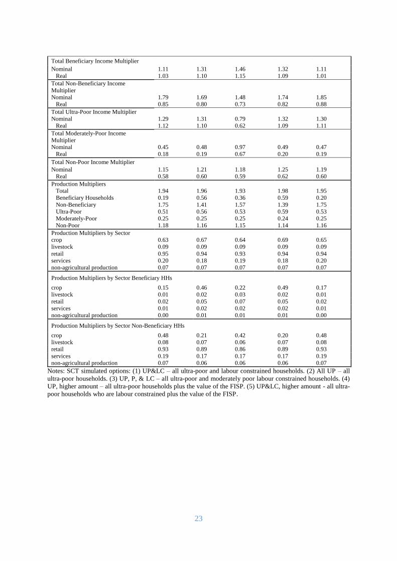
23
Total Beneficiary Income Multiplier
Nominal 1.11 1.31 1.46 1.32 1.11
Real 1.03 1.10 1.15 1.09 1.01
Total Non-Beneficiary Income
Multiplier
Nominal 1.79 1.69 1.48 1.74 1.85
Real 0.85 0.80 0.73 0.82 0.88
Total Ultra-Poor Income Multiplier
Nominal 1.29 1.31 0.79 1.32 1.30
Real 1.12 1.10 0.62 1.09 1.11
Total Moderately-Poor Income
Multiplier
Nominal 0.45 0.48 0.97 0.49 0.47
Real 0.18 0.19 0.67 0.20 0.19
Total Non-Poor Income Multiplier
Nominal 1.15 1.21 1.18 1.25 1.19
Real 0.58 0.60 0.59 0.62 0.60
Production Multipliers
Total 1.94 1.96 1.93 1.98 1.95
Beneficiary Households 0.19 0.56 0.36 0.59 0.20
Non-Beneficiary 1.75 1.41 1.57 1.39 1.75
Ultra-Poor 0.51 0.56 0.53 0.59 0.53
Moderately-Poor 0.25 0.25 0.25 0.24 0.25
Non-Poor 1.18 1.16 1.15 1.14 1.16
Production Multipliers by Sector
crop 0.63 0.67 0.64 0.69 0.65
livestock 0.09 0.09 0.09 0.09 0.09
retail 0.95 0.94 0.93 0.94 0.94
services 0.20 0.18 0.19 0.18 0.20
non-agricultural production 0.07 0.07 0.07 0.07 0.07
Production Multipliers by Sector Beneficiary HHs
crop 0.15 0.46 0.22 0.49 0.17
livestock 0.01 0.02 0.03 0.02 0.01
retail 0.02 0.05 0.07 0.05 0.02
services 0.01 0.02 0.02 0.02 0.01
non-agricultural production 0.00 0.01 0.01 0.01 0.00
Production Multipliers by Sector Non-Beneficiary HHs
crop 0.48 0.21 0.42 0.20 0.48
livestock 0.08 0.07 0.06 0.07 0.08
retail 0.93 0.89 0.86 0.89 0.93
services 0.19 0.17 0.17 0.17 0.19
non-agricultural production 0.07 0.06 0.06 0.06 0.07
Notes: SCT simulated options: (1) UP&LC – all ultra-poor and labour constrained households. (2) All UP – all
ultra-poor households. (3) UP, P, & LC – all ultra-poor and moderately poor labour constrained households. (4)
UP, higher amount – all ultra-poor households plus the value of the FISP. (5) UP&LC, higher amount - all ultra-
poor households who are labour constrained plus the value of the FISP.

24
Table 9. Percentage Impacts of SCT under Five Options
Percentage Changes (1) UP&LC (2)All UP (3) UP, P, &
LC
(4) UP, higher
amount
(5) UP&LC,
higher amount
Total Rural Income
Nominal 7.39% 17.80% 14.76% 26.55% 16.13%
(CI) (7.04%,
7.86%)
(16.83%,
19.10%)
(13.99%,
15.81%)
(24.91%,
28.65%)
(15.30%,
17.26%)
Real 5.06% 11.57% 9.82% 16.93% 10.82%
(CI) (4.81%,
5.37%)
(10.88%,
12.43%)
(9.28%,
10.49%)
(15.84%,
18.22%)
(10.24%,
11.54%)
Total Beneficiary Income
Nominal 47.29% 52.04% 37.57% 76.53% 101.54%
Real 44.11% 44.03% 31.66% 63.23% 92.41%
Total Non-Beneficiary
Income
Nominal 4.38% 11.38% 9.34% 17.17% 9.69%
Real 2.11% 5.47% 4.62% 8.24% 4.67%
Total Ultra-Poor Income
Nominal 23.51% 52.04% 28.40% 76.53% 50.66%
Real 20.84% 44.03% 22.91% 63.23% 43.83%
Total Moderately-Poor
Income
Nominal 3.68% 9.58% 19.76% 14.37% 8.08%
Real 1.46% 3.89% 14.70% 5.87% 3.24%
Total Non-Poor Income
Nominal 4.61% 12.01% 9.54% 18.16% 10.20%
Real 2.31% 6.03% 4.77% 9.07% 5.11%
Total Production 4.39% 11.24% 8.91% 16.56% 9.51%
Beneficiary Households 11.92% 32.19% 9.73% 48.97% 27.06%
Non-Beneficiary
Households 3.88% 7.57% 8.56% 10.88% 8.33%
Ultra-Poor Households 11.73% 32.19% 24.74% 48.97% 26.43%
Moderately-Poor
Households 2.91% 7.09% 5.75% 10.13% 6.12%
Non-Poor Households 3.21% 7.84% 6.36% 11.30% 6.78%
Production by Sector
crop 5.74% 15.36% 11.87% 22.97% 12.64%
livestock 2.35% 6.04% 4.80% 8.76% 5.02%
retail 3.88% 9.60% 7.75% 13.90% 8.26%
services 3.10% 7.24% 6.11% 10.57% 6.64%
non-agricultural production 3.93% 9.46% 7.69% 13.87% 8.44%
Production by Sector
Beneficiary HHs
crop 19.69% 53.27% 13.50% 81.99% 45.25%
livestock 2.72% 6.97% 4.87% 10.19% 5.80%
retail 5.99% 14.87% 10.17% 21.79% 12.89%
services 3.10% 7.23% 6.14% 10.64% 6.64%
non-agricultural production 4.31% 10.41% 8.03% 15.38% 9.26%
Production by Sector Non-
Beneficiary HHs
crop 4.53% 5.27% 11.07% 7.26% 9.81%
livestock 2.33% 5.89% 4.76% 8.53% 4.96%
retail 3.86% 9.39% 7.58% 13.58% 8.20%
services 3.10% 7.24% 6.10% 10.56% 6.64%
non-agricultural production 3.91% 9.38% 7.62% 13.74% 8.39%
Notes: SCT simulated options: (1) UP&LC – all ultra-poor and labour constrained households. (2) All UP – all
ultra-poor households. (3) UP, P, & LC – all ultra-poor and moderately poor labour constrained households. (4)
UP, higher amount – all ultra-poor households plus the value of the FISP. (5) UP&LC, higher amount - all utra-
poor households who are labour constrained plus the value of the FISP.

25
7.1.3 Policy options for the PWP LEWIE
The stand-alone PWP LEWIE policy options are presented below and summarized in Table 10.
1) Maintain the status quo: PWP to category II (C, E) and IV (G, H) households at current
coverage (12%) and transfer levels. 17
This PWP policy option reflects the current implementation of the programme, which consists
of providing 490 MK (US $0.68) per day, 4 hours per day, and 48 days per year. This
corresponds to a transfer income of approximately US $33 per year.
2) Ultra-poor targeting: Target category IV (G, H) at current transfer levels.
Simulate the rural economy-wide impact of improved targeting of the PWP. In this scenario the
public works to ALL ultra-poor households with labour capacity (assuming no exclusion
errors).
3) Increased duration of public works: Target categories II (C, E) and IV (G, H), current
coverage but higher number of days
The targeted group and the coverage are identical to the first PWP policy option but the total
number of days increased by twelve days. This implies a total transfer income of approximately
US $41.
Table 10. PWP Policy Options: Targeting, Coverage and Level of Benefits
Category Description Coverage as percentage
of total number of
households
Benefit
per day in
USD
Total transfer cost
without administrative
costs in 2016 MK
Option 1
(status quo by
end of 2017)
II (C,E) Wages paid to 55%
of moderately poor
and ultra-poor
labour -
unconstrained HH
Approx. 16 percent of the
total number of HHs,
about 450,000 HH
0.90 per
day, 48
days of
work
13 billion MK
IV (G, H)
Option 2
(ultra-poor
labour-
unconstrained
HHs)
IV (G, H)
Wages paid to 92%
of ultra-poor
labour -
unconstrained HH
Approx. 16 percent of the
total number of HHs,
about 450,000 HH
See option
1
13 billion MK
Option 3 (all
poor labour-
unconstrained
HHs with
more days)
II (C,E) Wages paid to 55%
of moderately poor
and ultra-poor
labour -
unconstrained HH
Approx. 16 percent of the
total number of HHs,
about 450,000 HH
0.90 per
day, 96
days of
work
25.9 billion MK
17 Coverage levels were obtained from the Local Development Fund of the Government of Malawi,
http://www.ldf.gov.mw.

26
These simulations are similar to what was done for the SCT, but some take into account
productivity impacts of public works projects.18 PWP impacts were simulated as a combination
of cash transfers to PWP participants and an increase in crop productivity resulting from the
creation of public goods . PWPs transfers increase incomes and thus expenditures in the targeted
households, setting in motion local economy-wide impacts captured by the LEWIE model.
PWPs also create public goods, which can increase productivity, in particular crop productivity
in households with access to land. It unclear how PWPs affect crop productivity through the
creation of public goods, because before-and-after data are not available.19
The only study the authors are aware of that estimates impacts of PWP on incomes and
productivity was carried out for the Ethiopia Productive Safety Net Programme (PSNP).20 It
found an average productivity impact of approximately 5%, with large variations across types
of public works projects and localities (kebeles) in which the public works projects were carried
out. The LEWIE model was used to simulate the rural economy-wide impacts of PWP with
cash transfers only (options 1a, 2a, and 3a). Simulations that combined this with an assumed
5% increase in crop productivity (Options 1b, 2b, and 3b) were also run. Implicitly, the “a”
options assume no productivity impact of PWP, and the “b” options assume a 5% productivity
impact. These are likely to bracket the extremes of PWP impacts.
7.1.4. Key findings for PWPs
The results are summarized in Tables 11 and 12. Table 11 presents income multipliers, which
as for the SCT multipliers only reflect transfer costs under the different scenarios. When
benefits are higher such as under Options 3a and 3b, so are costs, thus income multipliers may
not change. Table 12 presents percentage changes. Detailed multiplier and percentage results
are in Appendix B.
Overall, the nominal income multiplier effects of PWPs are similar to those of the SCT, except
if one assumes that PWPs can increase productivity through asset creation and skills transfers.
Total nominal income multipliers for options (Table 11) are on the order of 2.9, meaning that
each MK invested in the PWP increases total nominal income by 2.9 MK. However, real
multipliers diverge from the SCT when land productivity for programmes is increased as in
Options 1b, 2b, and 3b. This is due to additional benefits per MK of transfer generated by land
18 PWPs also transfer skills to beneficiary households which they may transfer to their own farms and/or
businesses. Due to the inherent heterogeneity of this knowledge transfer, the potential impact is not modelled. 19 Beegle et al. 2017 finds that PWPs in Malawi do not have an impact on beneficiary households and perhaps
negative spillovers to non-beneficiaries in villages that receive PWP wages, however the study does not look at
the impact of the rural assets (mainly road construction and irrigation) created. 20 Mateusz Filipski, J. Edward Taylor, Getachew Ahmed Abegaz, Tadele Ferede, Alemayehu Seyoum Taffesse,
and Xinshen Diao (2016). Economy-wide impacts of the Productive Safety Net Programme (PSNP). ESSP
RESEARCH NOTE 57 (July);
http://ebrary.ifpri.org/utils/getfile/collection/p15738coll2/id/130466/filename/130677.pdf

27
productivity increases. The total real (price-adjusted) income multipliers range from 1.89
(Option 1a) to 3.24 (Option 1b).
The largest income gains are for the targeted household groups, however income spillovers to
other household groups are also large and widespread. Targeted households benefit from the
PWP transfers as well as from the spillovers these transfers create. But spillovers also reach to
non-beneficiary households, including the non-poor. For every MK transferred the incomes of
non-beneficiaries increase in real terms by between 0.8 and 1.9 MK. Real income multipliers
are larger for non-beneficiaries when PWP increases productivity (Options b) as non-
beneficiaries also benefit directly from higher productivity results from community assets that
may have been created.
Production multipliers are large for both beneficiaries and non-beneficiaries and concentrated
in the retail and crop sector. The increase in retail production derives primarily from the
increased demand stimulated by the wage component, and benefit mostly non-beneficiaries
who are the owners of more retail assets. The increase in crop production involves beneficiaries
as well as non-beneficiary households and is higher when PWP also bring increased
productivity through assets and skills.
The direct transfer (through wage) and productivity increase (through the creation of rural assets
and training) effects of PWP are mutually reinforcing. The biggest impact of productivity
growth is to increase real income, because food prices fall when productivity rises. Public
works, by increasing the productivity of crop production, mitigate upward pressure on prices
caused by the cash transfers. Price increases from increased demand are offset by falling prices
due to increased supply. Production increases are especially high for crops. This simulation
demonstrates the importance of creating effective public work assets (and transferring skills
and knowledge through PWPs) to increase production and mitigate price inflation caused by
cash transfers.
The magnitude of income and production effects of PWPs depends on the quality of assets and
skills transferred and their relevance to increasing productivity in agriculture. If productivity
increases are smaller in Malawi than the 5% estimated in Ethiopia’s PSNP - for example
because the quality or type of asset produced is not adequate, or there is no sufficient focus on
skills transfers - total income under each option increases by a percentage amount that is in
between the “a” and “b” scenarios.
Income and production effects are larger if PWPs are available for a longer period and/or
provide a more generous wage. The largest percentage impacts (Table 11) occur under Option
3b, in which the PWP targets all poor labour-unconstrained HHs with the highest number of
days and productivity increases as a result. Total income increases by 6.6% in nominal terms
and 5.9% in real terms. This is the most expensive PWP scenario (it has the highest transfer
value), however, and because of this, the real income multipliers with productivity change are
higher under Options 1b and 2b than under 3b.

28
A narrower targeting of PWPs to ultra-poor with labour capacity has similar local economy
effects but different distributional implications. Options 1 and 2 deliver income and production
multipliers of similar magnitude but Option 2, which targets only ultra-poor with labour
capacity but leaving the total number of affected households unchanged, produces larger
percentage increases of the income and production of the ultra-poor.
Table 11. Multiplier Impacts of PWPs under Three Options
Option 1a (status
quo by end of
2017)
Option 1b (Option
1a with 5% Crop
Land Productivity
Increase)
Option 2a (ultra-
poor labour-
unconstrained
HHs)
Option 2b (Option
2a with 5% Crop
Land Productivity
Increase)
Option 3a (all
poor labour-
unconstrained
HHs with more
days)
Option 3b
(Option 3a with
5% Crop Land
Productivity
Increase)
Nominal 2.87 2.86 2.91 2.90 2.90 2.89
(CI) ( 2.74- 3.05) ( 2.73- 3.04) ( 2.78- 3.09) ( 2.77- 3.09) ( 2.76- 3.09) ( 2.75- 3.08)
Real 1.89 3.24 1.90 3.15 1.89 2.58
(CI) ( 1.80- 1.99) ( 3.16- 3.35) ( 1.82- 2.02) ( 3.07- 3.26) ( 1.80- 2.00) ( 2.50- 2.69)
Total Beneficiary Income Multiplier
Nominal 1.29 1.29 1.18 1.18 1.30 1.29
Real 1.13 1.41 1.08 1.24 1.12 1.27
Total Non-Beneficiary Income Multiplier
Nominal 1.58 1.57 1.73 1.72 1.60 1.60
Real 0.76 1.83 0.82 1.91 0.77 1.31
Total Ultra-Poor Income Multiplier
Nominal 0.88 0.88 1.29 1.29 0.89 0.89
Real 0.73 0.99 1.14 1.38 0.73 0.86
Total Moderately-Poor Income Multiplier
Nominal 0.85 0.85 0.46 0.46 0.86 0.86
Real 0.58 1.02 0.19 0.58 0.58 0.80
Total Non-Poor Income Multiplier
Nominal 1.14 1.13 1.15 1.15 1.15 1.15
Real 0.57 1.24 0.58 1.19 0.58 0.92
Production Multipliers
Total 1.94 3.26 1.96 3.17 1.95 2.62
Beneficiary Households 0.41 0.67 0.33 0.48 0.42 0.56
Non-Beneficiary 1.53 2.58 1.63 2.69 1.53 2.06
Ultra-Poor 0.51 0.76 0.52 0.76 0.52 0.66
Moderately-Poor 0.26 0.67 0.26 0.64 0.25 0.46
Non-Poor 1.18 1.83 1.18 1.77 1.17 1.50
Production Multipliers by Sector
crop 0.64 1.96 0.67 1.88 0.65 1.32
livestock 0.09 0.09 0.10 0.10 0.09 0.09
retail 0.95 0.95 0.95 0.96 0.95 0.95
services 0.19 0.19 0.18 0.18 0.19 0.19
non-agricultural production 0.07 0.07 0.07 0.07 0.07 0.07
Production Multipliers by Sector Beneficiary HHs
crop 0.29 0.55 0.27 0.42 0.29 0.43
livestock 0.01 0.01 0.01 0.01 0.01 0.01
retail 0.07 0.07 0.03 0.03 0.07 0.07
services 0.03 0.03 0.01 0.01 0.03 0.03
non-agricultural production 0.00 0.00 0.00 0.00 0.00 0.00
Production Multipliers by Sector Non-Beneficiary HHs
crop 0.36 1.41 0.39 1.45 0.36 0.89
livestock 0.07 0.07 0.08 0.08 0.07 0.07
retail 0.88 0.88 0.92 0.92 0.88 0.88
services 0.16 0.16 0.17 0.17 0.16 0.16
non-agricultural production 0.06 0.06 0.06 0.06 0.06 0.06
Household
Multipliers
Options
Total Income Multiplier

29
Table 12. Percentage Impacts of PWPs under Three Options
Household
Multipliers
Options
Option 1a
(status quo
by end of
2017)
Option 1b
(Option 1a
with 5% Crop
Land
Productivity
Increase)
Option 2a
(ultra-poor
labour-
unconstraine
d HHs)
Option 2b
(Option 2a
with 5%
Crop Land
Productivity
Increase)
Option 3a
(all poor
labour-
unconstraine
d HHs with
more days)
Option 3b
(Option 3a
with 5%
Crop Land
Productivity
Increase)
Total Income Multiplier
Nominal 2.87 2.86 2.91 2.90 2.90 2.89
(CI) ( 2.74- 3.05) ( 2.73- 3.04) ( 2.78- 3.09) ( 2.77- 3.09) (2.76- 3.09) ( 2.75- 3.08)
Real 1.89 3.24 1.90 3.15 1.89 2.58
(CI) ( 1.80- 1.99) ( 3.16- 3.35) ( 1.82- 2.02) ( 3.07- 3.26) (1.80- 2.00) ( 2.50- 2.69)
Total Beneficiary Income Multiplier
Nominal 1.29 1.29 1.18 1.18 1.30 1.29
Real 1.13 1.41 1.08 1.24 1.12 1.27
Total Non-Beneficiary Income Multiplier
Nominal 1.58 1.57 1.73 1.72 1.60 1.60
Real 0.76 1.83 0.82 1.91 0.77 1.31
Total Ultra-Poor Income Multiplier
Nominal 0.88 0.88 1.29 1.29 0.89 0.89
Real 0.73 0.99 1.14 1.38 0.73 0.86
Total Moderately-Poor Income Multiplier
Nominal 0.85 0.85 0.46 0.46 0.86 0.86
Real 0.58 1.02 0.19 0.58 0.58 0.80
Total Non-Poor Income Multiplier
Nominal 1.14 1.13 1.15 1.15 1.15 1.15
Real 0.57 1.24 0.58 1.19 0.58 0.92
Production Multipliers
Total 1.94 3.26 1.96 3.17 1.95 2.62
Beneficiary Households 0.41 0.67 0.33 0.48 0.42 0.56
Non-Beneficiary 1.53 2.58 1.63 2.69 1.53 2.06
Ultra-Poor 0.51 0.76 0.52 0.76 0.52 0.66
Moderately-Poor 0.26 0.67 0.26 0.64 0.25 0.46
Non-Poor 1.18 1.83 1.18 1.77 1.17 1.50
Production Multipliers by
Sector
crop 0.64 1.96 0.67 1.88 0.65 1.32
livestock 0.09 0.09 0.10 0.10 0.09 0.09
retail 0.95 0.95 0.95 0.96 0.95 0.95
services 0.19 0.19 0.18 0.18 0.19 0.19
non-agricultural production 0.07 0.07 0.07 0.07 0.07 0.07
Production Multipliers by
Sector Beneficiary HHs
crop 0.29 0.55 0.27 0.42 0.29 0.43
livestock 0.01 0.01 0.01 0.01 0.01 0.01
retail 0.07 0.07 0.03 0.03 0.07 0.07
services 0.03 0.03 0.01 0.01 0.03 0.03
non-agricultural production 0.00 0.00 0.00 0.00 0.00 0.00
Production Multipliers by
Sector Non-Beneficiary
HHs
crop 0.36 1.41 0.39 1.45 0.36 0.89
livestock 0.07 0.07 0.08 0.08 0.07 0.07
retail 0.88 0.88 0.92 0.92 0.88 0.88
services 0.16 0.16 0.17 0.17 0.16 0.16
non-agricultural production 0.06 0.06 0.06 0.06 0.06 0.06

30
7.2. Agricultural interventions
In addition to social protection programmes, the study also uses the LEWIE model to simulate
spillover effects of FISP, irrigation and extension. The impacts of FISP were simulated through
a decrease in crop input prices equal to the FISP subsidy for eligible households. For the FISP21,
irrigation and extension simulations, we first econometrically estimated the impacts of both on
predicted crop yields, then used the LEWIE model to estimate income and production spillovers
from the higher yields.
Table 13 reports the results of using household micro-data to estimate the impacts of FISP,
irrigation and extension on predicted crop yields for the households that benefit from FISP,
irrigation and/or extension. We estimated the model using various specifications. The study’s
econometric model estimates a Cobb-Douglas production function like the one used to estimate
the crop production parameters for the LEWIE model (Table 4), with household-group fixed
effects (poor/non-poor), other household characteristics, regional fixed effects, and dummy
variables indicating that a household received a FISP coupon, had access to irrigation and to
extension services. The estimations obtain robust standard errors using the Huber-White
sandwich estimator, to deal with potential problems related to heteroscedasticity and the
possibility of influential outliers.
Table 13. Econometric Estimates of Impacts of FISP, Irrigation and Extension on Yields
Variables Estimated coefficients
Log of hired labour days per hectare 0.196***
(0.0201)
Log of household labour days per hectare 0.466***
(0.0267)
Log of purchased inputs per hectare 0.0585***
(0.00778)
Log of crop assets per hectare 0.0790***
(0.0131)
Household used irrigated land 0.116***
(0.0370)
Household saw a government extension agent in the last 12 months 0.116**
(0.0484)
Household received a FISP coupon 0.239***
(0.0474)
Household is moderately or ultra-poor -0.301***
(0.0403)
Household characteristics including dummies for language spoken at home X
Household regional dummies X
Observations 7,212
R-squared 0.251 Note: Robust standard errors in parentheses. *** p<0.01, ** p<0.05, * p<0.1. HH characteristics include: HH head has attended
school, HH size, HH head is female, HH head has difficulties hearing, seeing, walking and/or chronically ill, dependency ratio,
HH head is less than 15 years old, HH head is 65 or older, dummy variables for languages spoken at home.
21 The reason the impact of the FISP on yields is simulated as well is that there may be an effect of the fertilizer
subsidy beyond the impact on purchased inputs; e.g. the use of fertilizer may act as technology adoption for low
yield farmers, making them more efficient. Throughout the text this effect is referred to as FISP with technology
change.

31
The econometric findings indicate that there are large and significant positive correlations
between FISP, irrigation, and extension interventions, on one hand, and crop yields, on the
other. At the same levels of factor (labour, land, capital) use, receiving a FISP coupon is
associated with a 23.9% increase in predicted yields – technology change increasing farmer
efficiency, access to irrigated land is associated with a 11.6% increase, and access to extension
raises crop yields by 11.6%.
7.2.1. Policy options for the FISP LEWIE
The stand-alone FISP LEWIE policy options are presented below and summarized in Table 14.
1) Maintain the status quo: FISP randomly provided to all household groups (A, B, C, D,
E, F, G, H, I and J) with current coverage 30% of all rural households, and the same
level of benefit (100kg bags of fertilizer with 80% subsidy).
This policy option aims to reflect the current implementation of FISP. It consists of providing
100kg bag of fertilizer to 900,000 households at a highly subsidized price.
2) Shift to “productive” farmers: FISP randomly provided to (above 1.5 acres) households
with land above 1.5 acres (A, C, D, G, and I) with current coverage 30% of all rural
households, and the same level of benefit (100kg bags of fertilizer with 80% subsidy).
This policy option aims to reflect Government of Malawi pilot studies that target FISP only to
those farm households with land above a “productive” threshold, considered as having access
to land above the median (above 1.5 acres). It consists of providing 100kg bag of fertilizer to
900,000 households with land above the median at a highly subsidized price.
3) Mixed pro-poor “productive” farmers targeting: Target moderately and ultra-poor
households with land above 1.5 acres (groups C, D, and G), with the same level of
benefits.
This policy provides an option to more narrowly target the FISP (hence reducing coverage and
cost) with the main focus more vulnerable “productive” farmers. With respect to FISP policy
option 2), this option excludes from FISP the two extreme categories of households with land
above 1.5 acres (the non-poor and the ultra-poor labour constrained). It provides the same level
of benefits, but to a smaller group of households (377,000 households): 100kg bags of fertilizer
with 80% subsidy to all households C, D, and G.
4) Mixed less poor “productive” farmers targeting: Target non-poor and moderately poor
households with land above 1.5 acres (groups A, C, and D), with the same level of
benefits.
This policy provides an alternative option to narrow focus of the FISP, in this case toward
better-off “productive” farmers. With respect to policy option 2), this option excludes from

32
FISP the poorest categories of households with land above 1.5 acres (ultra-poor with labour)
and includes non-poor households. It provides the same levels of benefits: 100kg bags of
fertilizer with 80% subsidy to all households A, C, and D.
5) Reduced subsidy level: Target non-poor and moderately poor households with land
above 1.5 (groups A, C, and D), with a lower level of benefits.
With respect to policy option 4), this option provides a lower level of benefits: 100kg bags of
fertilizer with 50% subsidy to all households A, C, and D. Coverage is left unchanged.
For each policy option we also generate a simulation that includes technology adoption due to
FISP. This is a result of our econometric estimations (explained in more detail in the next
section) which demonstrates that after controlling for a number of factors including the direct
effect of the subsidy through purchased inputs, there may be an added technological benefit on
yields of receiving FISP.
Table 14. FISP Policy Options: Targeting, Coverage and Level of Benefits
Category Description Coverage as %
of total number
of households
Transfer Subsidy Subsidy cost without
administrative cost in
2016 MK
Option 1
(status quo
by end of
2017)
All categories
of households
(A, B, C, D, E,
F, G, H, I, J)
FISP given to
all households
Approx. 32
percent of the
total number of
HHs, about
900,000 HH
100 Kg
bag of
fertilizer
80%
26.5 billion MK
Option 2
(“productiv
e farmers”)
All categories
of HHs with
land above 1.5
acres (A, C, D,
G, I)
FISP given to
all households
with land above
the median
Approx. 32
percent of the
total number of
HHs, about
900,000 HH
100 Kg
bag of
fertilizer
80%
26.5 billion MK
Option 3
(mixed pro-
poor
targeting)
More
vulnerable
”productive”
farmers ( C, D,
G)
FISP given to
all households
with land above
the median
excluding non-
poor and ultra-
poor labour-
constrained
Approx. 13
percent of the
total number of
HHs, about
377,000 HH
100 Kg
bag of
fertilizer
80%
11.1 billion MK
Option 4
(mixed less-
poor
targeting)
Less vulnerable
”productive”
farmers (A, C,
D)
FISP given to
all households
with land above
the median
excluding ultra-
poor
Approx. 24
percent of the
total number of
HHs, about
677,000 HH
100 Kg
bag of
fertilizer
80%
19.9 billion MK
Option 5
(mixed less-
poor
targeting,
less
subsidy)
Less vulnerable
”productive”
farmers (A C,
D)
A lower FISP
subsidy given
to all
households
with land above
the median
excluding ultra-
poor
Approx. 24
percent of the
total number of
HHs, about
677,000 HH
100 Kg
bag of
fertilizer
50%
12.4 billion MK

33
7.2.2. Key Findings for the FISP
The LEWIE simulations of rural economy-wide impacts of the five FISP options are
summarized in Tables 15 (multiplier effects, reflecting subsidy costs) and 16 (percentage
changes).22 Detailed multiplier and percentage results are in Appendix B.
Key lessons emerging from this analysis are presented below:
The FISP stimulates crop production in all five scenarios, and it increases both nominal
and real incomes of the targeted households. Crop output increases by 0.6% to 8.9% (Table
15) if we consider only the direct effects of the subsidies (the first column under each option).
However, when we include FISP in the regression reported in Table 15, we find that the FISP
is significantly correlated with crop yields, independent of the direct subsidy effect.23 This
suggests that FISP beneficiaries use different technologies to produce their crops. When we
consider the full effect, including technology change, crop output increases by 2% to 13.2%
(see second column underneath each option in Table 15). Real income impacts diverge from
nominal impacts because of changes in prices of local goods and services (including crop
prices). All poor households with land end up having a real income increase except in Option’s
4 and 5 when the poorest household groups are not recipients of the FISP.
Redirecting FISP toward households with land above the median increases crop
production and rural income. Recently the MoAIWD has experimented with redirecting FISP
toward more land rich farmers in a few districts. So far their studies have shown this to be more
effective than the current version of FISP. Our simulations appear to confirm these results.
Moving from Option 1 to Option 2, which keeps total coverage and subsidy level the same but
targets FISP toward households with land above the median, increases both overall crop
production and rural income. The impact of FISP without technology change increases from
15% to 8.2%. With technology change, the impact rises from 2.2% to 13.2%. Higher food
production puts downward pressure on food prices, increasing real (price-adjusted) incomes for
food consumers. Real income increases for all poverty groups (ultra-poor, moderately poor and
non-poor) because of lower food prices. Only household group J, the ultra-poor labour
constrained with land below the median, has a slightly lower real income under Option 2 than
Option 1. Total real income in rural Malawi increases from 1.67% to 3.34% without technology
change and from 2.49% to 5.14% with technology change under Option 2. It is important to
note that land rich households includes both ultra-poor and moderately poor households with
access to land, and both groups show positive income and production multipliers across all
scenarios.
22 These simulations, as in all of the simulations, include the effect of changes in crop production on crop prices.
Ricker-Gilbert et al. (2013) confirm that increased crop production reduces crop prices when they found that
roughly doubling the scale of FISP reduces maize prices by 1.8–2.8% on average. 23 The coefficient on the FISP dummy is significant at the 1% level after controlling for the direct impact of
purchased inputs on yields. Despite over a 24% impact on yields for FISP beneficiaries from our econometric
estimates, these are not experimental results and may be the result of a spurious correlation driven by
unobservables. Thus the study conservatively estimates only a 10% increase in yields, similar to irrigation and
extension, outside of the direct subsidy effect.

34
Targeting poor and ultra-poor farmers with access to land (the most vulnerable amongst
the “productive” farmers) in FISP, rather than better off farmers, produces larger income
and production multipliers for the economy as a whole. Options 3 and 4 imply a more
narrow coverage (and cost) of the FISP, comparing a more and less pro-poor targeting approach
while maintaining the focus on productive farmers (with land above the 1.5 acres). Real income
multipliers are larger across the board when FISP is maintained for ultra-poor and non-poor
farmers are excluded (Option 3), both for direct beneficiaries (7 MK vs. 3 MK, with
technological change) and for the rural economy as a whole (11.9 MK vs 2.8 MK with
technological change, 4 times as much). FISP is found to increase the crop production capacity
of the ultra-poor households with labour and land by between 66% and 117%. Instead when
this group is excluded from the programme (Option 4) their production capacity falls between
50% and 55%. Interestingly, non-poor households with land see their income increase in real
terms even when they do not directly receive FISP as they benefit from lower prices and
increase their production in other sectors (e.g. retail).
Interestingly, from an aggregate production perspective, targeting FISP to the most vulnerable
(ultra-poor and moderately poor) amongst the “productive” farmers with land (Option 3)
delivers a three times higher increase in the total volume of crops produced in the economy,
compared to a scenario (Option 4) where the subsidy is directed to better-off “productive”
farmers (24% versus an 8% percentage change, with technological change). This somewhat
surprising finding can primarily be explained by the different production functions of poor and
non-poor farmers. Non-poor farmers with land use relatively more land and capital than labour,
compared to the ultra-poor (with land). Since the model assumes that land and capital are fixed
factors that cannot be expanded in the short-term, non-poor farmers are somewhat less affected
by changes in input prices. Ultra-poor and poor farmers, on the other hand, respond to changes
in input prices mainly by expanding hired labour and family labour, which are more flexible,
thus increasing crop production. Moreover, as mentioned before ultra-poor households’ crop
production is negatively affected by the FISP when they are not directly targeted.
The FISP creates income spillovers for non-targeted households, but can also make them
worse off, which is problematic if the poorest farmers with land are excluded from the
programme. These income spillovers are large and positive in some cases, but frequently they
are negative for households that do not receive FISP subsidies, due to the effect on food prices.
Subsidized inputs stimulate crop production, and this drives down crop prices, which negatively
affects farmers who do not receive the subsidy. In all scenarios non-beneficiaries reduce crop
production and when poorest households are excluded from the programme (Options 4 and 5)
their real income is negatively affected. In this case FISP causes a net welfare loss for the poor
and can have potentially regressive distributional effects. When the FISP also impacts
technology, all real income for each household group becomes positive or are not significantly
different from zero.
Prices play a very important role in shaping the rural economy-wide impacts of FISP
subsidies. By causing production in FISP-beneficiary households to rise, the subsidies decrease
crop prices. Lower crop prices harm net sellers while benefiting net buyers, and they prevent
the increase in labour demand from being as large as it would be without price changes,

35
reducing real income for some household groups. The results in the second panel under each
option show that crop subsidies create benefits for some but negatively impact others in the
rural economy, unless they are combined with an increase in crop yields. This result may shed
light on the reasons why FISP has shown substantial impacts on yields in Malawi when the
rains have been steady (2005-2011) (Pauw and Thurow 2014) but has had little to no affect
during recent drought years when only the subsidy impact is present and the fertilizer induces
very little yield increase. Studies that do not consider price impacts miss much of the effect of
FISP subsidies.
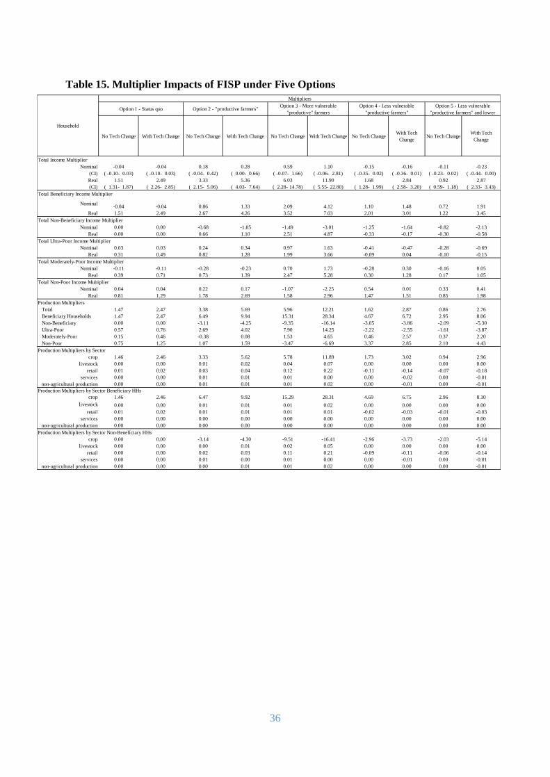
36
Table 15. Multiplier Impacts of FISP under Five Options
No Tech Change With Tech Change No Tech Change With Tech Change No Tech Change With Tech Change No Tech ChangeWith Tech
ChangeNo Tech Change
With Tech
Change
Nominal -0.04 -0.04 0.18 0.28 0.59 1.10 -0.15 -0.16 -0.11 -0.23
(CI) ( -0.10- 0.03) ( -0.10- 0.03) ( -0.04- 0.42) ( 0.00- 0.66) ( -0.07- 1.66) ( -0.06- 2.81) ( -0.35- 0.02) ( -0.36- 0.01) ( -0.23- 0.02) ( -0.44- 0.00)
Real 1.51 2.49 3.33 5.36 6.03 11.90 1.68 2.84 0.92 2.87
(CI) ( 1.31- 1.87) ( 2.26- 2.85) ( 2.15- 5.06) ( 4.03- 7.64) ( 2.28- 14.78) ( 5.55- 22.80) ( 1.28- 1.99) ( 2.58- 3.20) ( 0.59- 1.18) ( 2.33- 3.43)
Total Beneficiary Income Multiplier
Nominal-0.04 -0.04 0.86 1.33 2.09 4.12 1.10 1.48 0.72 1.91
Real 1.51 2.49 2.67 4.26 3.52 7.03 2.01 3.01 1.22 3.45
Total Non-Beneficiary Income Multiplier
Nominal 0.00 0.00 -0.68 -1.05 -1.49 -3.01 -1.25 -1.64 -0.82 -2.13
Real 0.00 0.00 0.66 1.10 2.51 4.87 -0.33 -0.17 -0.30 -0.58
Total Ultra-Poor Income Multiplier
Nominal 0.03 0.03 0.24 0.34 0.97 1.63 -0.41 -0.47 -0.28 -0.69
Real 0.31 0.49 0.82 1.28 1.99 3.66 -0.09 0.04 -0.10 -0.15
Total Moderately-Poor Income Multiplier
Nominal -0.11 -0.11 -0.28 -0.23 0.70 1.73 -0.28 0.30 -0.16 0.05
Real 0.39 0.71 0.73 1.39 2.47 5.28 0.30 1.28 0.17 1.05
Total Non-Poor Income Multiplier
Nominal 0.04 0.04 0.22 0.17 -1.07 -2.25 0.54 0.01 0.33 0.41
Real 0.81 1.29 1.78 2.69 1.58 2.96 1.47 1.51 0.85 1.98
Production Multipliers
Total 1.47 2.47 3.38 5.69 5.96 12.21 1.62 2.87 0.86 2.76
Beneficiary Households 1.47 2.47 6.49 9.94 15.31 28.34 4.67 6.72 2.95 8.06
Non-Beneficiary 0.00 0.00 -3.11 -4.25 -9.35 -16.14 -3.05 -3.86 -2.09 -5.30
Ultra-Poor 0.57 0.76 2.69 4.02 7.90 14.25 -2.22 -2.55 -1.61 -3.87
Moderately-Poor 0.15 0.46 -0.38 0.08 1.53 4.65 0.46 2.57 0.37 2.20
Non-Poor 0.75 1.25 1.07 1.59 -3.47 -6.69 3.37 2.85 2.10 4.43
Production Multipliers by Sector
crop 1.46 2.46 3.33 5.62 5.78 11.89 1.73 3.02 0.94 2.96
livestock 0.00 0.00 0.01 0.02 0.04 0.07 0.00 0.00 0.00 0.00
retail 0.01 0.02 0.03 0.04 0.12 0.22 -0.11 -0.14 -0.07 -0.18
services 0.00 0.00 0.01 0.01 0.01 0.00 0.00 -0.02 0.00 -0.01
non-agricultural production 0.00 0.00 0.01 0.01 0.01 0.02 0.00 -0.01 0.00 -0.01
Production Multipliers by Sector Beneficiary HHs
crop 1.46 2.46 6.47 9.92 15.29 28.31 4.69 6.75 2.96 8.10
livestock 0.00 0.00 0.01 0.01 0.01 0.02 0.00 0.00 0.00 0.00
retail 0.01 0.02 0.01 0.01 0.01 0.01 -0.02 -0.03 -0.01 -0.03
services 0.00 0.00 0.00 0.00 0.00 0.00 0.00 0.00 0.00 0.00
non-agricultural production 0.00 0.00 0.00 0.00 0.00 0.00 0.00 0.00 0.00 0.00
Production Multipliers by Sector Non-Beneficiary HHs
crop 0.00 0.00 -3.14 -4.30 -9.51 -16.41 -2.96 -3.73 -2.03 -5.14
livestock 0.00 0.00 0.00 0.01 0.02 0.05 0.00 0.00 0.00 0.00
retail 0.00 0.00 0.02 0.03 0.11 0.21 -0.09 -0.11 -0.06 -0.14
services 0.00 0.00 0.01 0.00 0.01 0.00 0.00 -0.01 0.00 -0.01
non-agricultural production 0.00 0.00 0.00 0.01 0.01 0.02 0.00 0.00 0.00 -0.01
Total Income Multiplier
Household
Multipliers
Option 1 - Status quo Option 2 - "productive farmers"Option 3 - More vulnerable
"productive" farmers
Option 4 - Less vulnerable
"productive farmers"
Option 5 - Less vulnerable
"productive farmers" and lower

37
Table 16. Percentage Impacts of FISP under Five Options
7.2.3. Policy options for extension services and irrigation
Policy options for the stand-alone LEWIE on extension services are presented below and
summarized in Table 17. Policy options for irrigation projects are summarized in Table 18.
1) Extension services provided to farmers with land above 1.5 acres (groups A, C, D, G,
and I) with increased visits of extension workers.
According to IHS3 data, 4% of households report having had a government extension worker
give them advice. This policy option consists of increasing the number of farmers accessing
extension services to farmers. Thus, this study assumes that an increase of visits by 100% which
implies a percentage of covered beneficiary farmers of 8%.
Table 17. Extension Services Policy Option: Targeting, Coverage and Level of Benefits
Policy option Category Coverage Benefits
Increase access to extension
services for households with
land above the median
I (A) Approx. 8% of rural
households, about 225,000
HHs (not equal across the 5
HHs categories)
Visits by additional
extension officers II (C)
III (D)
IV (G)
V (I)
No Tech Change With Tech Change No Tech Change With Tech Change No Tech Change With Tech Change No Tech Change With Tech Change No Tech ChangeWith Tech
Change
Total Rural Income
Nominal 0.19 0.18 0.26 0.19 0.17 0.06 -0.06 -0.34 -0.05 -0.39
(CI) ( -0.08, 0.45) ( -0.08, 0.44) ( -0.54, 1.15) ( -0.91, 1.48) ( -0.49, 0.94) ( -0.90, 1.24) ( -0.70, 0.52) ( -1.08, 0.45) ( -0.27, 0.13) ( -0.67, -0.10)
Real 1.67 2.61 3.34 5.14 1.74 3.16 1.61 2.62 0.53 1.35
(CI) ( 1.31, 2.12) ( 2.24, 3.05) ( 1.95, 5.28) ( 3.48, 7.61) ( 0.54, 4.38) ( 1.10, 6.90) ( 0.96, 2.24) ( 1.91, 3.70) ( 0.26, 0.77) ( 0.95, 1.73)
Total Beneficiary Income
Nominal 0.19 0.18 2.83 3.81 6.13 9.75 4.09 5.38 1.59 3.29
Real 1.67 2.61 6.59 9.92 8.19 13.94 6.13 9.09 2.28 5.41
Total Non-Beneficiary Income
Nominal NA NA -1.37 -2.10 -0.57 -1.14 -2.02 -3.05 -0.83 -2.13
Real NA NA 1.28 2.12 0.95 1.83 -0.53 -0.44 -0.30 -0.57
Total Ultra-Poor Income
Nominal 0.32 0.31 1.51 2.21 1.78 2.99 -2.58 -3.55 -1.12 -2.69
Real 2.19 3.36 5.44 8.57 3.82 7.05 -0.56 0.00 -0.41 -0.58
Total Moderately-Poor Income
Nominal 0.38 0.38 -0.82 -1.32 1.01 1.29 -0.55 -0.88 -0.26 -0.70
Real 2.15 3.27 2.81 4.50 2.91 5.05 1.40 2.59 0.43 1.34
Total Non-Poor Income
Nominal 0.09 0.08 0.32 0.20 -0.54 -1.12 0.75 0.66 0.29 0.30
Real 1.37 2.18 2.98 4.49 0.81 1.51 2.23 3.29 0.80 1.84
Total Production 1.03 2.20 8.24 13.18 5.01 9.92 1.71 4.06 0.56 2.47
Beneficiary Households 1.03 2.20 19.98 30.53 32.72 61.10 10.95 18.85 4.41 13.11
Non-Beneficiary Households NA NA -6.80 -9.07 -4.33 -7.35 -6.99 -9.86 -3.05 -7.55
Ultra-Poor Households 4.36 6.17 47.05 67.34 35.47 62.41 -20.58 -27.93 -9.26 -22.30
Moderately-Poor Households -0.05 1.54 -2.26 0.92 2.08 7.77 2.01 8.23 1.13 7.68
Non-Poor Households 0.73 1.49 3.49 5.23 -1.64 -3.17 7.60 10.46 2.92 6.32
Production by Sector
crop 4.94 8.44 17.68 28.42 12.86 24.33 3.74 8.35 1.09 4.39
livestock -0.05 -0.05 0.10 0.18 0.12 0.25 -0.05 -0.02 -0.02 0.00
retail 0.02 0.03 0.04 0.07 0.06 0.11 -0.18 -0.26 -0.08 -0.18
services 0.03 0.03 0.06 0.05 0.01 -0.01 0.01 -0.03 0.00 -0.04
non-agricultural production -0.01 -0.02 0.13 0.19 0.08 0.15 -0.10 -0.14 -0.05 -0.10
Production by Sector Beneficiary HHs
crop 4.94 8.44 49.09 74.27 76.13 137.98 30.36 49.92 11.98 33.41
livestock -0.05 -0.05 0.10 0.18 0.11 0.24 -0.05 -0.02 -0.02 0.00
retail 0.02 0.03 0.04 0.06 0.06 0.11 -0.18 -0.25 -0.07 -0.18
services 0.03 0.03 0.06 0.05 0.02 -0.02 0.02 -0.03 0.00 -0.04
non-agricultural production -0.01 -0.02 0.13 0.19 0.09 0.15 -0.10 -0.14 -0.05 -0.10
Production by Sector Non-Beneficiary HHs
crop NA NA -26.39 -35.91 -14.35 -24.54 -20.96 -30.20 -9.01 -22.53
livestock NA NA 0.10 0.18 0.12 0.25 -0.05 -0.02 -0.02 0.00
retail NA NA 0.04 0.07 0.06 0.11 -0.18 -0.26 -0.08 -0.18
services NA NA 0.06 0.05 0.01 -0.01 0.01 -0.03 0.00 -0.04
non-agricultural production NA NA 0.13 0.19 0.08 0.15 -0.10 -0.14 -0.05 -0.11
Percentage Changes
Option 1 - Status quo Option 2 - "productive farmers"Option 3 - More vulnerable
"productive" farmers
Option 4 - Less vulnerable
"productive farmers"
Option 5 - Less vulnerable
"productive farmers" and lower
subsidy

38
2) Irrigation projects provided to farmers with land above 1.5 acres (groups A, C, D, G,
I) but with an increase in percentage of total land equipped for irrigation.
FAOSTAT states that 1.3% of the agricultural land in the country is equipped for irrigation.
According to the IHS3 data, 17% of agricultural households reported having access to
irrigation. One of the main aim of the draft National Agricultural Investment Plan (formally
known as ASWAp) 2015-2035 is to achieve 210,000 ha of irrigated land, which corresponds
approximately to 4% of total agricultural land. If the percentage of households with access to
irrigation increases proportionally to the increase of irrigated land (approximately doubling),
we should expect the percentage of households with access to irrigation to reach approximately
34% (from a current 17%) of agricultural households.
Table 18 Irrigation Policy Option: Targeting, Coverage and Level of Benefits
Policy option Category Coverage Benefits
Increase access to irrigated
land for households with
land above the median
I (A) Approx. 34% of rural HHs, about
960,000 HHs (not equally
distributed across the 5 HHs
groups)
Irrigated land: 4%
of the total
agricultural land II (C)
III (D)
IV (G)
V (I)
7.2.4. Key findings for extension services and irrigation
We used the econometric estimates of direct effects of extension and irrigation (Table 13),
together with the LEWIE model, to simulate the rural economy-wide impacts of an increase in
access to extension services from 4% to 8% of rural households with land above 1.5 acres (A,
C, D, G, and I), and an increase in access to irrigation from 17% to 34% of households with
land above 1.5 acres. The simulations take into account impacts of increased productivity on
crop prices. It also takes into account the amounts of money given to rural workers in the
process of administrating the programme(s).
Experts from the FAO investment center estimate that for irrigation projects, generally 20% to
30% of the cost ends up as wages for rural workers.24 We therefore used the estimate of 30%
as a transfer, combined with the impact on land productivity. Since the costs of irrigation are
high, and spread out over 20 years, we used two different estimates of costs. One is the full cost
of increasing irrigation from 17% to 34% as well as the costs of rehabilitating and maintaining
all irrigation projects, US$2,424 million but divided by the 20 year span envisioned for
approximately doubling irrigation, and two is the annual cost of maintaining and operating
irrigation once this project is fully completed, US$278 million (Chafuwa, 2017). 30% of these
amounts are included as a transfer to rural households with land.
Extension services were estimated to cost approximately US$ 21 million for 2016/17 (GoM
2017). Even more extensively than for irrigation, much of the money spent on extension goes
back to the rural local economy in the form of wages to extension workers. For Malawi, there
24 Actual amounts vary by irrigation project, and by year, and are beyond the scope of this paper. This is merely
to highlight the need to include, in the estimate of benefits, the cash given back to the rural community in the form
of rural wages.

39
are no estimates of the percentage of wages for rural workers as opposed to money spent in
urban areas. The study therefore uses percentages estimated from extension costs in nearby
Zambia to estimate rural impacts. The wages amount to 92% of costs or US$ 19.2 million. The
simulations include this amount as a transfer to rural households with land above 1.5 acres and
include the direct effects of extension on yields.
The resulting multiplier changes in incomes and production appear in Table 19. The percentage
counterpart to this table is in Table 20. These multipliers are also the cost-benefit multipliers
since they include the administrative as well as transfer costs (they cannot be separated as in
the case of the previous policy programmes). Detailed multiplier and percentage results are in
Appendix B.
Table 19. Multiplier Impacts and Cost-benefit Ratios of Extension Services and
Irrigation
MultipliersIrrigation (Full
Cost)
Irrigation (Annual
Cost)Extension
Total Income Multiplier
Nominal 0.87 0.89 2.63
(CI) ( 0.83- 0.93) ( 0.85- 0.96) ( 2.51- 2.80)
Real 0.85 0.69 2.07
(CI) ( 0.78- 0.96) ( 0.65- 0.76) ( 1.98- 2.24)
Total Beneficiary Income Multiplier
Nominal 0.67 0.62 1.86
Real 0.68 0.53 1.61
Total Non-Beneficiary Income Multiplier
Nominal 0.20 0.27 0.77
Real 0.17 0.16 0.46
Total Ultra-Poor Income Multiplier
Nominal 0.18 0.18 0.53
Real 0.18 0.16 0.46
Total Moderately-Poor Income Multiplier
Nominal 0.21 0.21 0.63
Real 0.22 0.16 0.48
Total Non-Poor Income Multiplier
Nominal 0.48 0.50 1.48
Real 0.45 0.38 1.12
Production Multipliers
Total 0.86 0.71 2.10
Beneficiary Households 0.83 0.50 1.45
Non-Beneficiary 0.03 0.21 0.65
Ultra-Poor 0.18 0.17 0.41
Moderately-Poor 0.20 0.13 0.42
Non-Poor 0.48 0.41 1.27
Production Multipliers by Sector
crop 0.47 0.32 0.91
livestock 0.03 0.03 0.09
retail 0.28 0.28 0.86
services 0.06 0.06 0.18
non-agricultural production 0.02 0.02 0.06
Production Multipliers by Sector Beneficiary HHs
crop 0.73 0.40 1.14
livestock 0.02 0.02 0.05
retail 0.06 0.06 0.18
services 0.02 0.02 0.05
non-agricultural production 0.01 0.01 0.02
Production Multipliers by Sector Non-Beneficiary HHs
crop -0.25 -0.08 -0.23
livestock 0.01 0.01 0.04
retail 0.22 0.22 0.68
services 0.04 0.04 0.13
non-agricultural production 0.01 0.01 0.04

40
Table 20. Percentage Impacts of Extension Services and Irrigation
Doubling the share of households (with land above 1.5 acres) with access to irrigation
results in an increase in crop production of 9.55% (full cost annualized) and 15.58%
Percentage ChangesIrrigation (Full
Cost, annualized)
Irrigation (Annual
Cost)Extension
Total Rural Income
Nominal 6.09 14.66 3.18
(CI) ( 5.65, 6.65) ( 13.75, 15.98) ( 3.01, 3.41)
Real 5.87 11.30 2.48
(CI) ( 5.33, 6.75) ( 10.50, 12.62) ( 2.33, 2.71)
Total Beneficiary Income
Nominal 11.28 24.09 5.33
Real 11.43 20.87 4.69
Total Non-Beneficiary Income
Nominal 2.82 8.71 1.83
Real 2.37 5.27 1.09
Total Ultra-Poor Income
Nominal 8.61 20.44 4.40
Real 8.91 17.46 3.80
Total Moderately-Poor Income
Nominal 4.36 11.20 2.45
Real 4.55 8.43 1.85
Total Non-Poor Income
Nominal 6.06 14.41 3.13
Real 5.57 10.76 2.37
Total Production 9.55 15.58 3.29
Beneficiary Households 18.09 25.05 5.25
Non-Beneficiary Households -1.41 3.44 0.78
Ultra-Poor Households 24.27 42.32 7.56
Moderately-Poor Households 8.84 12.61 2.96
Non-Poor Households 5.93 9.96 2.31
Production by Sector
crop 15.75 24.10 4.89
livestock 2.43 5.43 1.23
retail 3.66 8.40 1.90
services 2.94 6.81 1.53
non-agricultural production 3.64 8.34 1.86
Production by Sector Beneficiary HHs
crop 38.17 49.05 10.09
livestock 2.40 5.35 1.22
retail 3.67 8.43 1.91
services 2.94 6.81 1.53
non-agricultural production 3.69 8.46 1.89
Production by Sector Non-Beneficiary HHs
crop -15.71 -10.92 -2.42
livestock 2.49 5.57 1.26
retail 3.66 8.39 1.90
services 2.94 6.81 1.53
non-agricultural production 3.61 8.29 1.85

41
(annual cost once operational) as well as a 5.87% (full cost annualized) and 11.3% (annual cost
once operational) increase in total real income that is significant at well above the 95% level.
The nominal income effect due to the transfer and productivity increase is even higher (6.09%
and 14.66% respectively). Households with irrigation benefit, however, by driving down the
price of crops, non-beneficiaries decrease their crop production. Still, real incomes rise across
households because the cost of food consumption decreases with larger crop output and
spillovers benefit all households. Irrigation creates spillovers to other production sectors as
well.
Not surprisingly, there are large income increases for the household groups with land
above 1.5 acres targeted by new irrigation projects, but the spillover effects on real income
in households with land below 1.5 acres are also large. Increases in real income exceed 14%
for some groups (C, G, and I). For the groups with land below 1.5 acres, those who receive the
spillovers but not the direct effects, the real income increases are smaller but still significant.
For ultra-poor groups, both those with direct access to irrigation and those who receive only
spillovers, real income gains range from 2.45% (J) to 34% (G, I, under the annual cost once
operational simulation). This simulation demonstrates the potentially large and far-reaching
impact of irrigation for the rural economy of Malawi.
The real-income and production impacts of extension are smaller but positive. Total real
income rises by 2.48%, and this increase is statistically significant. There are only small
spillovers to other production sectors; however, real incomes increase for all household groups.
Real incomes rise by as much as 7% in the ultra-poor households (G and I). Access to extension
services, like irrigation, creates real benefits that extend beyond crop production.
The multiplier table (Table 19) shows also the multipliers of irrigation and extension.
Extension has both real income and production multipliers that are above 2 MK per MK
spent. Thus, even though the percentage increases in real income and production due to
extension is lower than for irrigation, the benefit of 1 MK spent on extension is more than for
1 MK spent on irrigation. Even if costs are born by households with land above 1.5 acres (as is
the case with those who receive extension services in this simulation), they still have positive
income. Extension services is a programme that tends to benefit workers in rural areas
(extension agents), who contribute to the local economy by spending their wage on products
and services from those locations.
Irrigation on the other hand has smaller multipliers and in fact a lower than one cost-
benefit ratio for both real income and production. The reason for this is the high capital cost
of irrigation infrastructure purchased outside the local economy. However, the multipliers do
not capture the benefits of lower crop prices that urban consumers receive due to irrigation
improvements nor the resulting increase in food security and exports. This may be significant
given crop production increases of 16% rising to 24% once completed (Table 20). Moreover,
Malawi has seen a rise in smallholder irrigation schemes (Chafuwa, 2017). This may be a more
cost-effective approach to expanding irrigation and increasing cost-benefit ratios.
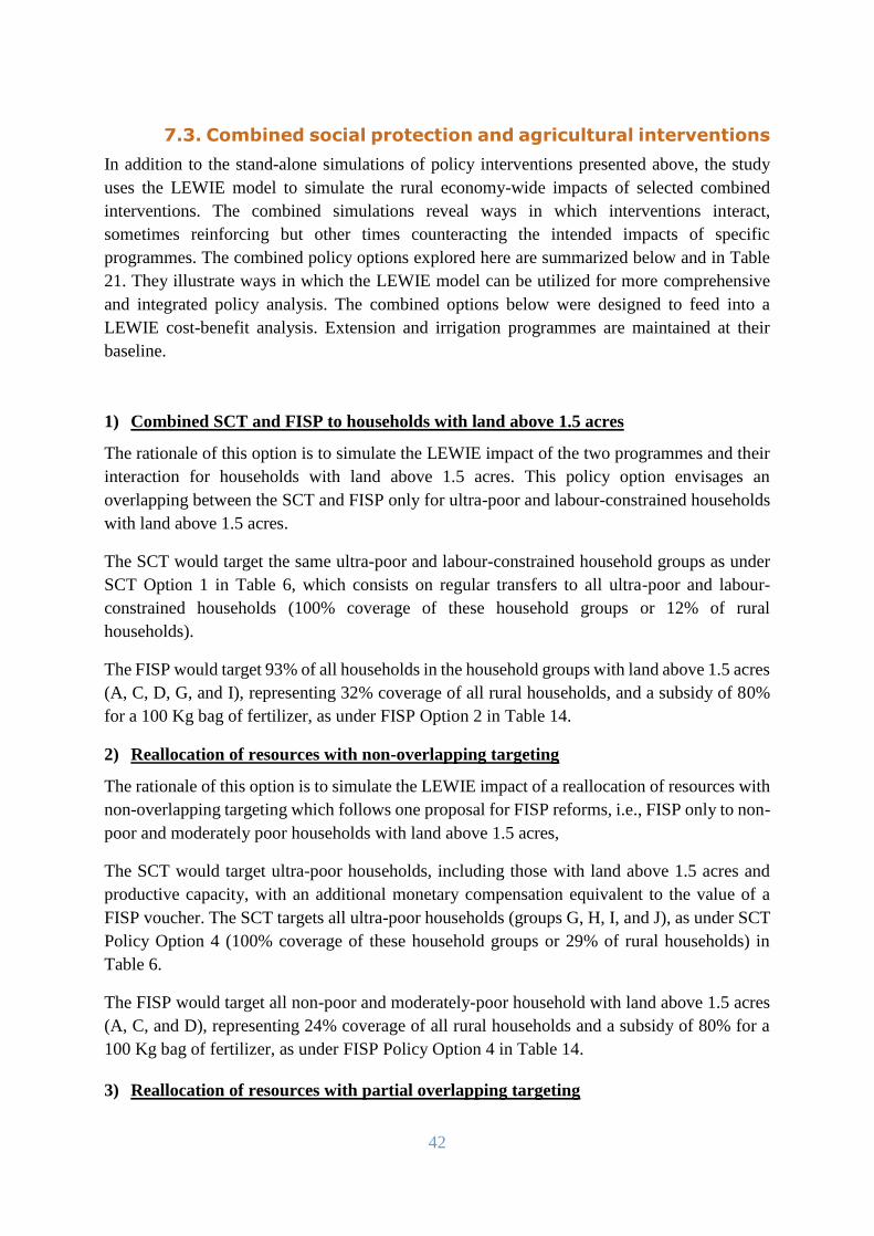
42
7.3. Combined social protection and agricultural interventions
In addition to the stand-alone simulations of policy interventions presented above, the study
uses the LEWIE model to simulate the rural economy-wide impacts of selected combined
interventions. The combined simulations reveal ways in which interventions interact,
sometimes reinforcing but other times counteracting the intended impacts of specific
programmes. The combined policy options explored here are summarized below and in Table
21. They illustrate ways in which the LEWIE model can be utilized for more comprehensive
and integrated policy analysis. The combined options below were designed to feed into a
LEWIE cost-benefit analysis. Extension and irrigation programmes are maintained at their
baseline.
1) Combined SCT and FISP to households with land above 1.5 acres
The rationale of this option is to simulate the LEWIE impact of the two programmes and their
interaction for households with land above 1.5 acres. This policy option envisages an
overlapping between the SCT and FISP only for ultra-poor and labour-constrained households
with land above 1.5 acres.
The SCT would target the same ultra-poor and labour-constrained household groups as under
SCT Option 1 in Table 6, which consists on regular transfers to all ultra-poor and labour-
constrained households (100% coverage of these household groups or 12% of rural
households).
The FISP would target 93% of all households in the household groups with land above 1.5 acres
(A, C, D, G, and I), representing 32% coverage of all rural households, and a subsidy of 80%
for a 100 Kg bag of fertilizer, as under FISP Option 2 in Table 14.
2) Reallocation of resources with non-overlapping targeting
The rationale of this option is to simulate the LEWIE impact of a reallocation of resources with
non-overlapping targeting which follows one proposal for FISP reforms, i.e., FISP only to non-
poor and moderately poor households with land above 1.5 acres,
The SCT would target ultra-poor households, including those with land above 1.5 acres and
productive capacity, with an additional monetary compensation equivalent to the value of a
FISP voucher. The SCT targets all ultra-poor households (groups G, H, I, and J), as under SCT
Policy Option 4 (100% coverage of these household groups or 29% of rural households) in
Table 6.
The FISP would target all non-poor and moderately-poor household with land above 1.5 acres
(A, C, and D), representing 24% coverage of all rural households and a subsidy of 80% for a
100 Kg bag of fertilizer, as under FISP Policy Option 4 in Table 14.
3) Reallocation of resources with partial overlapping targeting

43
The rationale of this option is to simulate the local economy impacts of a reallocation of
resources with partial overlapping targeting between SCT and FISP.
The SCT would target all ultra and moderately-poor households without labour capacity
(groups D, F, I, and J), as under SCT Option 3 (100% coverage of these household groups or
20% of rural households) in Table 6.
The FISP would target more vulnerable “productive” farmers with land above 1.5 acres,
including the ultra-poor (groups C, D, and G), representing 13% coverage of rural households
and a subsidy of 80% for a 100 Kg bag of fertilizer, as under FISP Policy Option 4 in Table 14.
4) Reallocation of resources with fully overlapping targeting of vulnerable “productive”
farmers
The rationale of this option is to simulate the local economy impacts of a reallocation of
resources with fully overlapping targeting between SCT and FISP.
FISP would target more vulnerable “productive” farmers with land above 1.5 acres, including
the ultra-poor (groups C, D, and G), representing 13% coverage of rural households and a
subsidy of 80% for a 100 Kg bag of fertilizer, as under FISP Option 4 in Table 14.
The SCT would target the same household groups as those who received the FISP, in this case
all C, D, and G households.
5) Reallocation of resources with fully overlapping targeting of ultra-poor households
The rationale of this option is to simulate the local economy impacts of a reallocation of
resources with fully overlapping targeting between SCT and FISP, but to all ultra-poor
households.
FISP would target the ultra-poor (groups G, H, I and J), representing 29% coverage of rural
households and a subsidy of 80% for a 100 Kg bag of fertilizer.
The SCT would target the same household groups as those who received the FISP, in this case
all ultra-poor households G, H, I, and J households, corresponding to SCT Option 2 (100%
coverage of these household groups or 29% of rural households) in Table 6.
Two different variants to each option are simulated, a total of fifteen simulations. First, the FISP
is simulated to directly impact yields by an amount equal to the estimated impact in Table 14
(called “With Tech Change” Options). Second, the PWP targeting groups C, E, G, and H, with
16% coverage of all rural households, as under PWP Option 1 in Table 9. (“W/ PWP No Tech
Change”) are added. Detailed results of these additional simulations are included in Appendix
B.

44
Table 21. Summary of Combined Simulations of Social Protection and Agricultural
Interventions
COMBINED POLICIES SCT FISP PWP
OPTION 1:
combined
SCT and
FISP HHs
with land
above 1.5
acres
Specific policy SCT policy 1 FISP policy 2 PWP policy 1
Targeting I A C
J C E
D G
G H
I
Coverage as a
% of total
number of HHs
Approx. 12% of the total
number of HHs, about
330,000 HH.
Approx. 32% of the total
number of HHs, about
900,000 HH
Approx. 16% of the total
number of HHs, about
450,000 HH
Benefits Weighted average of current
transfers
100 Kg bag of fertilizer
(80% subsidy)
0.90 per day, 48 days of
work
Total Cost 62.7 billion MWK (SCT: 27.7 billion, FISP: 26.5 billion, PWP: 8.6 billion)
OPTION 2:
reallocation
of resources
with non-
overlapping
targeting
Specific policy SCT policy 4 FISP policy 4 PWP Policy 1
Targeting G A C
H C E
I D G
J H
Coverage as a
% of total
number of HHs
Approx. 29% of the total
number of HHs, about
820,000 HHs
Approx. 24% of the total
number of HHs, about
677,000 HHs
Approx. 16% of the total
number of HHs, about
450,000 HHs
Benefits Weighted average of current
transfers + monetary value of
FISP
100 Kg bag of fertilizer
(80% subsidy)
0.90 per day, 48 days of
work
Total Cost 128.8 billion MWK (SCT: 100.3 billion, FISP: 19.9 billion, PWP: 8.6 billion)
OPTION 3:
reallocation
of resources
with partial
overlapping
targeting
Specific policy SCT policy 3 FISP policy 3 PWP Policy 1
Targeting D C C
F D E
I G G
J H
Coverage as a
% of total
number of HHs
Approx. 20% of the total
number of HHs, about
560,000 HHs
Approx. 13% of the total
number of HHs, about
377,000 HHs
Approx. 16% of the total
number of HHs, about
450,000 HHs
Benefits Weighted average of current
transfers
100 Kg bag of fertilizer
(80% subsidy)
0.90 per day, 48 days of
work
Total Cost 75.8 billion MWK (SCT: 56.1 billion, FISP: 11.1 billion, PWP: 8.6 billion
OPTION 4:
Fully
overlapping
targeting of
vulnerable
"productive
" farmers
Specific policy SCT overlapping with FISP FISP policy 3 PWP Policy 1
Targeting C C C
D D E
G G G
H
Coverage as a
% of total
number of HHs
Approx. 13% of the total
number of HHs, about
377,000 HHs
Approx. 13% of the total
number of HHs, about
377,000 HHs
Approx. 16% of the total
number of HHs, about
450,000 HHs
Benefits Weighted average of current
transfers
100 Kg bag of fertilizer
(80% subsidy)
0.90 per day, 48 days of
work
Total Cost 51.3 billion MWK (SCT: 31.6 billion, FISP: 11.1 billion, PWP: 8.6 billion)
OPTION 5:
Fully
overlapping
targeting to
ultra-poor
households
Specific policy SCT Policy 2 FISP overlapping with
SCT
PWP Policy 1
Targeting H H C
I I E
J
J
G
H
Coverage as a
% of total
number of HHs
Approx. 29% of the total
number of HHs, about
820,000 HHs
Approx. 29% of the total
number of HHs, about
820,000 HHs
Approx. 16% of the total
number of HHs, about
450,000 HHs
Benefits Weighted average of current
transfers
100 Kg bag of fertilizer
(80% subsidy)
0.90 per day, 48 days of
work
Total Cost 94 billion MWK (SCT: 68.8 billion, FISP: 16.6 billion, PWP: 8.6 billion)

45
7.3.1. Key findings for combined social protection and agricultural interventions
Four important lessons emerge from this analysis of combined policy options.
The SCT mitigates negative impacts of FISP on food prices. In the stand-alone simulations
that consider crop price impacts, the FISP stimulates crop production and puts downward
pressure on crop prices. This results in increases in real income, but a slight decrease in nominal
incomes for some groups that earn income from growing crops, either as farm operators or
agricultural workers. The SCT raises incomes in SCT-targeted households, and this stimulates
the demand for food and other goods in the rural economy. The positive income spillovers that
this new demand creates counteract all of the negative nominal income impacts of FISP. The
impacts on total nominal incomes range from 7.4% (option 4 with technological change) to
around 30% (option 2 with PWP).
The FISP enhances the real-income effects of the SCT. Without FISP, the demand stimulus
created by the SCT puts upward pressure on crop prices, which raises consumption costs in
SCT beneficiary and non-beneficiary households. With FISP, there is an increased food supply
to meet the demand, and this mitigates the impact of the SCT on food costs. Other interventions
that stimulate food production, e.g., irrigation and extension, have a similarly complementary
influence on the real-income impacts of the SCT25, so this finding does not necessarily mean
that FISP is the best productive interaction to raise the impact of the SCT. The real (inflation-
adjusted) total income impacts range from 6.6% (Option 4 without technological change) to
20.2% (Option 2 with PWP).
Technology change induced by the FISP considerably enhances the impacts of other
policy interventions. This becomes evident by comparing the real income impacts of each
option with and without the technology changes from FISP reported in Table 15, which were
estimated econometrically then fed through the LEWIE model. Technological change raises the
real-income impact for each option while increasing crop production, sometimes by more than
10 percentage points such as in Option 3 (from 26.6% to 37.65%).
Policy options with the SCT and FISP partially or fully overlapping have higher real
income and production multipliers compared to when programmes are implemented in
isolation. Real income and production multipliers in simulations where the targeting of the SCT
and FISP does not overlap (Option 2) are lower than those of partially overlapping simulations
(Option 3), which again are lower than the fully overlapping simulations (Option 4 and Option
5). A full overlap of FISP and SCT targeting to the ultra-poor not only produces higher
multipliers for the whole economy compared to partial and non-overlapping targeting, but also
has a better distributional impact, with larger increases in incomes and production amongst the
poorest households. These findings highlight the existence of synergies that could enhance
25 Simulations for SCT + PWP + Irrigation and SCT + PWP + Extension for option 1 instead of FISP produce
similar results as with the FISP. They are not reported but available upon request.

46
programmes’ effectiveness through the deliberate targeting of productive and protective
interventions to the same household groups.
Table 22. Multiplier Results of LEWIE Simulations of Combined Policy Interventions
No Tech Change With Tech ChangeW/ PWP No Tech
ChangeNo Tech Change With Tech Change
W/ PWP No
Tech ChangeNo Tech Change
With Tech
Change
W/ PWP No
Tech ChangeNo Tech Change With Tech Change
W/ PWP No
Tech ChangeNo Tech Change
With Tech
Change
W/ PWP No
Tech Change
Total Income Multiplier
Nominal 2.07 2.10 2.30 2.73 2.71 2.77 2.79 2.82 2.85 2.70 2.74 2.77 2.93 2.98 2.95
(CI) ( 1.92- 2.24) ( 1.93- 2.29) ( 2.13- 2.48) ( 2.57- 2.95) ( 2.55- 2.90) ( 2.61- 3.01) ( 2.62- 3.00) ( 2.61- 3.06) ( 2.67- 3.06) ( 2.54- 2.92) ( 2.55- 2.99) ( 2.59- 2.97) ( 2.77- 3.15) ( 2.78- 3.24) ( 2.76- 3.16)
Real 2.38 3.01 2.25 1.83 1.97 1.84 2.15 2.47 2.09 2.36 3.01 2.20 2.23 2.66 2.19
(CI) ( 1.96- 3.01) ( 2.51- 3.70) ( 1.93- 2.79) ( 1.79- 1.89) ( 1.92- 2.02) ( 1.79- 1.89) ( 1.84- 2.77) ( 2.01- 3.29) ( 1.83- 2.62) ( 1.92- 3.36) ( 2.23- 4.26) ( 1.87- 2.87) ( 2.01- 2.48) ( 2.37- 2.95) ( 1.99- 2.41)
Total Beneficiary Income Multiplier
Nominal 1.60 1.74 1.78 1.96 2.02 2.04 1.61 1.74 1.77 1.49 1.70 1.60 1.35 1.44 1.46
Real 1.85 2.36 1.83 1.45 1.61 1.46 1.4 1.65 1.45 1.42 1.81 1.43 1.23 1.41 1.28
Total Non-Beneficiary Income Multiplier
Nominal 0.47 0.35 0.52 0.76 0.69 0.74 1.18 1.08 1.08 1.22 1.04 1.17 1.58 1.54 1.5
Real 0.53 0.65 0.42 0.39 0.36 0.38 0.75 0.82 0.64 0.94 1.20 0.76 1 1.24 0.9
Total Ultra-Poor Income Multiplier
Nominal 0.98 1.00 0.96 1.13 1.09 1.11 0.81 0.85 0.83 0.79 0.86 0.82 1.35 1.44 1.29
Real 1.07 1.22 0.98 0.96 0.96 0.92 0.72 0.82 0.71 0.76 0.95 0.74 1.23 1.41 1.15
Total Moderately-Poor Income Multiplier
Nominal 0.23 0.24 0.39 0.41 0.42 0.46 0.95 1.02 0.94 0.98 1.08 0.95 0.44 0.42 0.5
Real 0.35 0.55 0.41 0.19 0.25 0.23 0.79 0.95 0.74 0.91 1.22 0.80 0.27 0.36 0.32
Total Non-Poor Income Multiplier
Nominal 0.86 0.86 0.95 1.19 1.20 1.21 1.03 0.95 1.08 0.94 0.80 1.01 1.15 1.13 1.16
Real 0.95 1.24 0.86 0.68 0.77 0.68 0.65 0.71 0.64 0.70 0.85 0.65 0.73 0.88 0.71
Production Multipliers
Total 2.45 3.19 2.33 1.89 2.03 1.90 2.21 2.56 2.15 2.41 3.13 2.25 2.29 2.78 2.26
Beneficiary Households 2.48 3.56 1.87 1.08 1.29 1.12 1.33 1.99 1.22 2.02 3.49 1.45 1.3 2.13 1.27
Non-Beneficiary -0.03 -0.37 0.46 0.81 0.74 0.78 0.88 0.57 0.93 0.39 -0.36 0.80 0.99 0.65 0.99
Ultra-Poor 1.26 1.68 1.06 0.18 -0.05 0.20 1.03 1.33 0.91 1.36 2.11 1.08 1.3 2.13 1.22
Moderately-Poor 0.05 0.19 0.10 0.30 0.44 0.29 0.31 0.54 0.31 0.38 0.69 0.35 0.1 -0.04 0.12
Non-Poor 1.14 1.32 1.16 1.42 1.64 1.40 0.87 0.69 0.93 0.67 0.33 0.83 0.89 0.69 0.92
Production Multipliers by Sector
crop 1.52 2.25 1.31 0.75 0.91 0.75 0.99 1.34 0.92 1.23 1.93 1.04 1.04 1.5 1
livestock 0.06 0.07 0.07 0.08 0.08 0.08 0.09 0.09 0.09 0.09 0.10 0.09 0.09 0.09 0.09
retail 0.67 0.68 0.74 0.83 0.82 0.84 0.89 0.89 0.89 0.86 0.87 0.88 0.92 0.94 0.92
services 0.14 0.14 0.15 0.17 0.17 0.17 0.18 0.18 0.18 0.17 0.17 0.18 0.18 0.18 0.18
non-agricultural production 0.05 0.05 0.06 0.06 0.06 0.06 0.06 0.07 0.07 0.06 0.06 0.06 0.07 0.07 0.07
Production Multipliers by Sector Beneficiary HHs
crop 2.23 3.31 1.52 0.73 0.94 0.73 1.17 1.83 0.98 1.93 3.40 1.28 1.21 2.04 1.12
livestock 0.04 0.04 0.05 0.06 0.06 0.06 0.04 0.04 0.04 0.03 0.03 0.03 0.02 0.02 0.02
retail 0.15 0.15 0.20 0.21 0.21 0.23 0.09 0.09 0.14 0.04 0.04 0.09 0.05 0.05 0.09
services 0.04 0.05 0.07 0.06 0.06 0.08 0.02 0.02 0.05 0.01 0.01 0.04 0.02 0.02 0.04
non-agricultural production 0.02 0.02 0.02 0.02 0.02 0.02 0.01 0.01 0.02 0.01 0.01 0.01 0.01 0.01 0.01
Production Multipliers by Sector Non-Beneficiary HHs
crop -0.71 -1.06 -0.21 0.02 -0.04 0.02 -0.18 -0.49 -0.05 -0.70 -1.47 -0.24 -0.17 -0.54 -0.11
livestock 0.02 0.03 0.02 0.03 0.03 0.03 0.05 0.05 0.04 0.06 0.07 0.06 0.07 0.07 0.07
retail 0.53 0.53 0.53 0.62 0.61 0.60 0.8 0.8 0.76 0.81 0.83 0.79 0.87 0.89 0.83
services 0.09 0.09 0.08 0.11 0.11 0.09 0.16 0.16 0.13 0.16 0.16 0.14 0.16 0.16 0.14
non-agricultural production 0.03 0.03 0.04 0.04 0.04 0.04 0.05 0.05 0.05 0.05 0.06 0.05 0.06 0.06 0.06
Household
Multipliers
Option 1: SCT + FISP to HHs with more than 1.5 acres
Option 2: Reallocation of resources with non-
overlapping targeting
Option 3: Reallocation of resources with partial
overlapping targeting
Option 4: Reallocation of resources with fully
overlapping targeting
Option 5: Reallocation of resources with fully
overlapping targeting to ultra-poor

47
Table 23. Percentage Results of LEWIE Simulations of Combined Policy Interventions
No Tech Change With Tech ChangeW/ PWP No Tech
ChangeNo Tech Change With Tech Change
W/ PWP No Tech
ChangeNo Tech Change With Tech Change
W/ PWP No Tech
ChangeNo Tech Change With Tech Change
W/ PWP No Tech
ChangeNo Tech Change With Tech Change
W/ PWP No Tech
Change
Total Rural Income
Nominal 7.62 7.54 11.05 26.32 25.92 29.99 14.88 14.73 18.45 7.57 7.40 10.95 18.29 18.66 21.84
(CI) ( 6.59%, 8.82%) ( 6.25%, 9.12%) ( 9.86%, 12.51%) ( 24.60%, 28.86%) ( 24.15%, 27.98%)( 28.01%, 32.80%)( 13.62%, 16.49%)( 13.08%, 16.82%)( 16.85%, 20.52%) ( 6.66%, 8.67%) ( 6.20%, 8.91%) ( 9.78%, 12.44%) ( 17.09%, 19.93%)( 17.14%, 20.84%)( 20.19%, 23.77%)
Real 8.59 10.47 10.82 18.04 19.02 20.24 11.71 12.97 13.85 6.56 8.13 8.65 14.05 16.64 16.37
(CI) ( 7.00%, 11.09%) ( 8.52%, 13.30%) ( 9.11%, 13.38%) ( 17.06%, 19.34%) ( 17.95%, 20.21%)( 19.15%, 21.73%)( 10.04%, 14.89%)( 10.51%, 17.24%)( 12.16%, 17.19%) ( 5.13%, 9.59%) ( 5.62%, 12.07%) ( 7.27%, 11.54%) ( 12.53%, 15.85%)( 14.57%, 19.02%)( 14.70%, 18.31%)
Total Beneficiary Income
Nominal 13.83 14.74 15.69 37.65 38.54 39.34 27.51 28.40 30.19 32.48 36.28 17.45 56.08 59.85 45.61
Real 15.49 18.89 16.15 28.97 31.58 29.30 24.41 27.15 25.62 31.64 38.09 15.42 51.24 58.68 39.87
Total Non-Beneficiary Income
Nominal 3.04 2.21 5.60 15.91 14.32 19.00 8.83 8.19 11.32 4.50 3.83 7.02 11.20 10.93 13.68
Real 3.49 4.24 4.54 8.00 7.48 9.59 5.63 6.18 6.70 3.47 4.43 4.54 7.07 8.74 8.30
Total Ultra-Poor Income
Nominal 25.15 25.70 31.28 72.73 70.23 79.01 30.36 31.52 36.67 14.85 16.15 20.98 56.08 59.85 62.63
Real 27.20 30.64 31.96 61.88 61.80 66.11 27.28 30.45 31.88 14.24 17.89 18.92 51.24 58.68 56.14
Total Moderately-Poor Income
Nominal 2.81 2.19 7.47 13.86 13.43 18.67 20.70 21.03 25.52 10.26 10.46 14.90 9.03 8.49 13.78
Real 4.36 5.96 7.90 6.77 7.79 10.19 17.81 19.91 21.11 9.62 11.95 12.91 5.61 7.50 9.21
Total Non-Poor Income
Nominal 4.87 4.81 7.18 18.93 19.07 21.54 8.90 8.24 11.32 4.78 4.09 7.02 11.96 11.79 14.32
Real 5.35 6.94 6.47 10.88 12.12 12.14 5.60 6.08 6.70 3.54 4.31 4.54 7.59 9.18 8.79
Total Production 13.45 18.70 15.62 17.37 19.46 19.42 14.67 19.44 16.62 10.70 16.26 12.44 16.03 21.14 18.05
Beneficiary Households 24.32 34.85 22.10 21.04 25.00 22.82 30.25 45.39 29.23 42.99 75.03 23.26 81.05 131.73 61.86
Non-Beneficiary Households -2.01 -4.25 2.63 11.00 9.87 12.60 4.05 1.77 6.22 -0.20 -3.57 3.52 4.65 1.78 6.00
Ultra-Poor Households 64.79 86.15 70.25 16.23 -4.58 20.73 65.93 88.77 70.02 53.89 85.38 56.68 81.05 131.73 87.09
Moderately-Poor Households 0.46 3.68 1.85 13.61 21.44 14.87 7.52 14.54 9.17 5.38 11.19 6.82 2.54 -1.97 3.70
Non-Poor Households 6.67 8.66 8.37 19.75 24.90 21.58 4.68 3.30 6.22 1.90 0.28 3.52 5.81 3.86 7.21
Production by Sector
crop 25.25 36.49 28.16 24.44 28.10 27.24 26.63 37.60 29.11 21.20 34.26 23.13 27.29 40.79 30.28
livestock 2.43 2.53 3.54 8.64 8.67 9.65 4.87 5.03 5.96 3.11 3.20 4.13 6.18 6.33 7.23
retail 3.94 3.96 5.74 13.65 13.48 15.38 7.85 7.84 9.60 4.45 4.52 6.24 9.78 9.99 11.55
services 3.12 3.13 4.54 10.58 10.52 11.97 6.08 6.08 7.53 3.43 3.38 4.83 7.34 7.39 8.73
non-agricultural production 4.06 4.10 5.82 13.62 13.60 15.44 7.76 7.79 9.52 4.33 4.39 6.07 9.70 9.89 11.43
Production by Sector Beneficiary HHs
crop 53.68 78.09 42.15 34.48 42.29 35.82 61.35 94.12 54.47 94.96 164.77 44.96 146.96 247.12 107.85
livestock 2.42 2.53 3.60 8.71 8.75 9.67 4.94 5.07 6.11 3.05 3.19 4.23 7.16 7.29 7.93
retail 3.98 3.98 6.31 14.64 14.53 17.11 10.03 10.26 13.00 4.62 4.53 8.40 15.19 15.18 16.45
services 3.17 3.22 4.59 10.69 10.70 11.96 6.13 6.04 7.50 3.42 3.41 4.81 7.35 7.52 8.85
non-agricultural production 4.10 4.16 5.89 13.95 13.85 15.89 8.15 8.31 10.18 4.39 4.43 6.48 10.69 10.84 12.50
Production by Sector Non-Beneficiary HHs
crop -20.81 -30.89 -11.51 1.94 -3.70 2.93 -5.48 -14.67 -2.35 -10.52 -21.88 -3.95 -4.56 -14.12 -3.95
livestock 2.44 2.53 3.39 8.46 8.48 9.58 4.81 4.99 5.83 3.13 3.20 4.04 6.02 6.17 7.06
retail 3.93 3.95 5.54 13.34 13.14 14.78 7.61 7.57 9.12 4.44 4.52 5.94 9.56 9.78 11.17
services 3.10 3.09 4.50 10.52 10.42 11.99 6.07 6.09 7.54 3.43 3.38 4.84 7.34 7.37 8.70
non-agricultural production 4.04 4.07 5.79 13.45 13.47 15.19 7.65 7.65 9.32 4.32 4.39 5.94 9.61 9.81 11.30
Percentage ChangesOption 1: SCT + FISP to HHs with more than 1.5 acres
Option 2: Reallocation of resources with non-
overlapping targeting
Option 3: Reallocation of resources with partial
overlapping targeting
Option 4: Reallocation of resources with fully
overlapping targeting
Option 5: Reallocation of resources with fully
overlapping targeting to ultra-poor

48
No Tech Change With Tech ChangeW/ PWP No Tech
ChangeNo Tech Change With Tech Change
W/ PWP No Tech
ChangeNo Tech Change With Tech Change
W/ PWP No Tech
ChangeNo Tech Change With Tech Change
W/ PWP No Tech
ChangeNo Tech Change With Tech Change
W/ PWP No Tech
Change
Total Rural Income
Nominal 7.62 7.54 11.05 26.32 25.92 29.99 14.88 14.73 18.45 7.57 7.40 10.95 18.29 18.66 21.84
(CI) ( 6.59%, 8.82%) ( 6.25%, 9.12%) ( 9.86%, 12.51%) ( 24.60%, 28.86%) ( 24.15%, 27.98%)( 28.01%, 32.80%)( 13.62%, 16.49%)( 13.08%, 16.82%)( 16.85%, 20.52%) ( 6.66%, 8.67%) ( 6.20%, 8.91%) ( 9.78%, 12.44%) ( 17.09%, 19.93%)( 17.14%, 20.84%)( 20.19%, 23.77%)
Real 8.59 10.47 10.82 18.04 19.02 20.24 11.71 12.97 13.85 6.56 8.13 8.65 14.05 16.64 16.37
(CI) ( 7.00%, 11.09%) ( 8.52%, 13.30%) ( 9.11%, 13.38%) ( 17.06%, 19.34%) ( 17.95%, 20.21%)( 19.15%, 21.73%)( 10.04%, 14.89%)( 10.51%, 17.24%)( 12.16%, 17.19%) ( 5.13%, 9.59%) ( 5.62%, 12.07%) ( 7.27%, 11.54%) ( 12.53%, 15.85%)( 14.57%, 19.02%)( 14.70%, 18.31%)
Total Beneficiary Income
Nominal 13.83 14.74 15.69 37.65 38.54 39.34 27.51 28.40 30.19 32.48 36.28 17.45 56.08 59.85 45.61
Real 15.49 18.89 16.15 28.97 31.58 29.30 24.41 27.15 25.62 31.64 38.09 15.42 51.24 58.68 39.87
Total Non-Beneficiary Income
Nominal 3.04 2.21 5.60 15.91 14.32 19.00 8.83 8.19 11.32 4.50 3.83 7.02 11.20 10.93 13.68
Real 3.49 4.24 4.54 8.00 7.48 9.59 5.63 6.18 6.70 3.47 4.43 4.54 7.07 8.74 8.30
Total Ultra-Poor Income
Nominal 25.15 25.70 31.28 72.73 70.23 79.01 30.36 31.52 36.67 14.85 16.15 20.98 56.08 59.85 62.63
Real 27.20 30.64 31.96 61.88 61.80 66.11 27.28 30.45 31.88 14.24 17.89 18.92 51.24 58.68 56.14
Total Moderately-Poor Income
Nominal 2.81 2.19 7.47 13.86 13.43 18.67 20.70 21.03 25.52 10.26 10.46 14.90 9.03 8.49 13.78
Real 4.36 5.96 7.90 6.77 7.79 10.19 17.81 19.91 21.11 9.62 11.95 12.91 5.61 7.50 9.21
Total Non-Poor Income
Nominal 4.87 4.81 7.18 18.93 19.07 21.54 8.90 8.24 11.32 4.78 4.09 7.02 11.96 11.79 14.32
Real 5.35 6.94 6.47 10.88 12.12 12.14 5.60 6.08 6.70 3.54 4.31 4.54 7.59 9.18 8.79
Total Production 13.45 18.70 15.62 17.37 19.46 19.42 14.67 19.44 16.62 10.70 16.26 12.44 16.03 21.14 18.05
Beneficiary Households 24.32 34.85 22.10 21.04 25.00 22.82 30.25 45.39 29.23 42.99 75.03 23.26 81.05 131.73 61.86
Non-Beneficiary Households -2.01 -4.25 2.63 11.00 9.87 12.60 4.05 1.77 6.22 -0.20 -3.57 3.52 4.65 1.78 6.00
Ultra-Poor Households 64.79 86.15 70.25 16.23 -4.58 20.73 65.93 88.77 70.02 53.89 85.38 56.68 81.05 131.73 87.09
Moderately-Poor Households 0.46 3.68 1.85 13.61 21.44 14.87 7.52 14.54 9.17 5.38 11.19 6.82 2.54 -1.97 3.70
Non-Poor Households 6.67 8.66 8.37 19.75 24.90 21.58 4.68 3.30 6.22 1.90 0.28 3.52 5.81 3.86 7.21
Production by Sector
crop 25.25 36.49 28.16 24.44 28.10 27.24 26.63 37.60 29.11 21.20 34.26 23.13 27.29 40.79 30.28
livestock 2.43 2.53 3.54 8.64 8.67 9.65 4.87 5.03 5.96 3.11 3.20 4.13 6.18 6.33 7.23
retail 3.94 3.96 5.74 13.65 13.48 15.38 7.85 7.84 9.60 4.45 4.52 6.24 9.78 9.99 11.55
services 3.12 3.13 4.54 10.58 10.52 11.97 6.08 6.08 7.53 3.43 3.38 4.83 7.34 7.39 8.73
non-agricultural production 4.06 4.10 5.82 13.62 13.60 15.44 7.76 7.79 9.52 4.33 4.39 6.07 9.70 9.89 11.43
Production by Sector Beneficiary HHs
crop 53.68 78.09 42.15 34.48 42.29 35.82 61.35 94.12 54.47 94.96 164.77 44.96 146.96 247.12 107.85
livestock 2.42 2.53 3.60 8.71 8.75 9.67 4.94 5.07 6.11 3.05 3.19 4.23 7.16 7.29 7.93
retail 3.98 3.98 6.31 14.64 14.53 17.11 10.03 10.26 13.00 4.62 4.53 8.40 15.19 15.18 16.45
services 3.17 3.22 4.59 10.69 10.70 11.96 6.13 6.04 7.50 3.42 3.41 4.81 7.35 7.52 8.85
non-agricultural production 4.10 4.16 5.89 13.95 13.85 15.89 8.15 8.31 10.18 4.39 4.43 6.48 10.69 10.84 12.50
Production by Sector Non-Beneficiary HHs
crop -20.81 -30.89 -11.51 1.94 -3.70 2.93 -5.48 -14.67 -2.35 -10.52 -21.88 -3.95 -4.56 -14.12 -3.95
livestock 2.44 2.53 3.39 8.46 8.48 9.58 4.81 4.99 5.83 3.13 3.20 4.04 6.02 6.17 7.06
retail 3.93 3.95 5.54 13.34 13.14 14.78 7.61 7.57 9.12 4.44 4.52 5.94 9.56 9.78 11.17
services 3.10 3.09 4.50 10.52 10.42 11.99 6.07 6.09 7.54 3.43 3.38 4.84 7.34 7.37 8.70
non-agricultural production 4.04 4.07 5.79 13.45 13.47 15.19 7.65 7.65 9.32 4.32 4.39 5.94 9.61 9.81 11.30
Percentage ChangesOption 1: SCT + FISP to HHs with more than 1.5 acres
Option 2: Reallocation of resources with non-
overlapping targeting
Option 3: Reallocation of resources with partial
overlapping targeting
Option 4: Reallocation of resources with fully
overlapping targeting
Option 5: Reallocation of resources with fully
overlapping targeting to ultra-poor

49
8. Local economy-wide cost-benefit analysis
Cost-benefit analysis (CBA) entails summing up the future stream of discounted benefits from
a project and comparing it with project costs. The formula for calculating the discounted net
benefits of a project, relative to the baseline without the project, is:
0 (1 )
t t
p npTt
tt
Y Y INPV
r
where )( npp
ttYY denote benefits with (without) the project, r is the discount rate, and
tI is the
project cost in year t.
The potential benefits of social protection and productive programmes are complex,
encompassing income gains (derived from a variety of channels) to beneficiary households,
income spillovers to non-beneficiary households, as well as other impacts to which it is difficult
to assign economic values (e.g., optimism about the future and happiness). Development
interventions potentially have a medium and long term impact on income in beneficiary
households. In the case of a SCT, the short-run income impact for beneficiaries equals the
amount of the transfer. For a PWP, it is the income spent on the project, which includes
payments to workers and other project inputs. Other interventions may increase income in the
short run by enhancing productivity in agricultural and/or nonagricultural activities. Long-run
impacts include the effects of human capital investments on productivity and incomes (e.g.,
once newly educated children grow up, farmers implement what they learn from agricultural
extension agents, new irrigation projects come on line, etc.). The study focusses only on the
economic benefits, specifically, income gains. Although income is a subset of all potential
benefits, it is the component that lends itself to CBA.
A critical difference between this and conventional CBA is that it incorporates the local
economy-wide benefits of the project, including income spillovers to non-beneficiaries. Income
spillovers to non-beneficiaries can be simulated with the use of a LEWIE model. Yp is the output
from our LEWIE model. The study compares these local-economy benefits, appropriately
discounted, to the cost of the programme. This local-economy CBA allows us to calculate the
net present value of the project, taking into account the programme’s impacts on income and
local economy-wide spillovers. If desired, it can be compared to the results of a CBA that
ignores spillovers.
To sum up, the CBA consists of annually calculating the benefits (total income benefits to
beneficiaries and non-beneficiaries including spillovers) over a time horizon, discounting these
benefits, adding up the discounted future stream of benefits and comparing it to the discounted
stream of project costs. The discounted stream of benefits is the present value (PV) of local-
economy benefits from the programmes mentioned. The discounted stream of programme costs
over this period (C) is the total amount transferred in the base year continuing on over the time
period, plus administrative costs. We subtract C from PV to obtain the net present value (NPV)
of a programme. The net benefit ratio (PV/C) gives the economic return per MK invested.

50
8.1. Cost-benefit ratios of the SCT
Table 24 presents a LEWIE CBA for SCT Option 1, using the real income multipliers reported
in Table 8 and shown in Figure 4. All numbers in this table are millions of 2016 MK.
The total amount of cash transferred to eligible households per year under Option 1 (assuming
full coverage of ultra-poor and labour-constrained groups I and J) is MK 27,656 million
(Column A). Column B gives the discounted value of the programme cost in each of the next
10 years, including administrative costs, using a discount rate of 10%. The costs, used above
when calculating the denominators of the multipliers in Table 23 include only transfer costs,
for the cost-benefit analysis we also include operation costs. For irrigation and extension part
of these costs include salaries paid to rural households. For the SCT, the study conservatively
estimates implementation costs equal to 26% of the value of the transfer. 26
The indirect income spillover effects of the transfers are given in Column C. Recovering the
multiplier from Table 8, under Option 1, each MK of the SCT increases total real income by
1.88 MK - that is, by the MK transferred plus an additional 0.88 MK of spillover. The indirect
spillover, then, is the 0.88 spillover times the total amount transferred, or MK 24,338 million
per year. This spillover is reported in Column C of Table 24.
Total discounted real-income benefits of the SCT under Option 1 are reported in Column D.
They include the amount transferred (Column A) plus the spillovers (Column C), discounted
each year at the discount rate of 10%. Their sum over ten years is MK 351,427 million.
One can compare these discounted benefits to the total discounted cost of the transfers over 10
years, which is MK 235,531 million. The differences between discounted benefits and costs
each year are given in Column E. Over the ten-year period, the SCT programme under option
1 creates total discounted benefits, net of transfer and admin costs, equal to MK 115,896
million. This represents a return of MK 1.49 per MK transferred to eligible households.
Table 24. LEWIE Cost-benefit Analysis of SCT Option 1
Years A B C D E
Amount transferred
to eligible households
Discounted SCT
cost, including
administration
Real income
spillover
Discounted benefits
including spillovers
Discounted
net benefit
1 27,656 34,847 24,338 51,994 17,147
2 27,656 31,679 24,338 47,267 15,588
3 27,656 28,799 24,338 42,970 14,171
4 27,656 26,181 24,338 39,064 12,883
5 27,656 23,801 24,338 35,512 11,712
6 27,656 21,637 24,338 32,284 10,647
7 27,656 19,670 24,338 29,349 9,679
8 27,656 17,882 24,338 26,681 8,799
9 27,656 16,256 24,338 24,255 7,999
10 27,656 14,778 24,338 22,050 7,272
Total 276,563 235,531 243,375 351,427 115,896
Ratio of Discounted Benefits to Discounted Costs: 351,427 / 235,531: 1.49 Notes: All figures are in millions of 2016 MK. This analysis assumes an annual discount rate of 10%, 26% administrative
cost, and a ten-year time horizon, with no changes in SCT transfers (in nominal terms) over the period.
26 Administrative costs given from 2015/2016 data from the Ministry of Gender, Children, Disability, and Social
Welfare (MoGCDSW).

51
This LEWIE CBA has been repeated for each of the other SCT options. Because the real income
multipliers in Table 24 are similar across the five SCT options, there is little difference in cost-
benefit ratios across the options. All are on the order of 1.49 to 1.52.
Nominal cost-benefit ratios, those based on the nominal SCT multipliers from Table 8 are
higher - on the order of 2.29 MK per MK of programme cost. This suggests that complementary
interventions targeted at raising productivity in rural areas and limiting price increases can
enhance the economic returns to SCT investments. This would cause real multipliers to
converge to higher nominal multipliers.
8.2. Cost-benefit ratios of PWPs
Table 25 presents results of a LEWIE CBA of the PWP Option 1. This option also includes
administrative costs and costs of tools and planning associated with this programme.27 Under
this option the total amount transferred to eligible households, in the form of wages for PWPs,
is MK 12,960 million. Administrative costs and tools add 67% to this amount. The LEWIE
analysis reveals real income spillovers of 0.89 MK per MK of programme cost, or a total of
MK 11,534 million per year. Total discounted benefits, including spillovers, equal MK 165,558
over the 10-year period. Dividing this by the total discounted programme costs yields a net
return of 1.13 per MK invested in PWPs.
Table 25. LEWIE Cost-benefit Analysis of PWP Option 1
Years A B C D E
Amount transferred
to eligible
households
Discounted PWP
cost, including
administration
Real income
spillover
Discounted benefits
including spillovers
Discounted
net benefit
1 12,960 21,643 11,534 24,494 2,851
2 12,960 19,676 11,534 22,268 2,592
3 12,960 17,887 11,534 20,243 2,356
4 12,960 16,261 11,534 18,403 2,142
5 12,960 14,783 11,534 16,730 1,947
6 12,960 13,439 11,534 15,209 1,770
7 12,960 12,217 11,534 13,826 1,609
8 12,960 11,106 11,534 12,570 1,463
9 12,960 10,097 11,534 11,427 1,330
10 12,960 9,179 11,534 10,388 1,209
Total 129,600 146,287 115,344 165,558 19,271
Ratio of Discounted Benefits to Discounted Costs: 165,558 / 146,287 1.13 Notes: All figures are in millions of 2016 MK. This analysis assumes an annual discount rate of 10%, 67% of the transfer on
administrative and cost of tools, and a ten-year time horizon, with no changes in PWP transfers (in nominal terms) over the
period.
These results highlight a number of relevant findings:
PWP policy options that assume the programme increases agriculture productivity have
significantly larger cost-benefit ratio. The highest cost-benefit ratios in the table, 1.94 and
27 Administrative costs plus the costs of tools for construction of the assets are assumed to be 67% of transfer costs.
This is typically the cost of the PWP however reforms are in process that may reduce this amount (Local
Development Fund of the Republic of Malawi).

52
1.89, correspond to projects resulting in an increase in land productivity and highest LEWIE
income multipliers. It is critical that PWP prioritize the creation of quality assets and transfer
skills that can lead to productivity gains, or otherwise the discounted benefits of PWP barely
exceed the costs of the programme (1.13 MK discounted benefit for 1 MK spent).
There are large overhead costs to PWPs, and because of this the cost-benefit ratios are
smaller for PWP than for the SCT with similar income multipliers. PWPs in general is less
efficient than the SCT at allocating transfers to poor households. Thus, the need for the creation
of quality agricultural assets and transfer skills through PWPs, is even more important given
the PWPs inherent inefficiencies in providing transfers.
Table 26. LEWIE Cost-benefit Analysis of PWP Options
PWP options Real income
multiplier
Cost-benefit
ratio
Option 1a (status quo by end of 2017) 1.89 1.13
Option 1b (Option 1a w 5% increase in land productivity) 3.24 1.94
Option 2a (ultra-poor labour-unconstrained HHs) 1.90 1.14
Option 2b (Option 2a w 5% increase in land productivity) 3.15 1.89
Option 3a (all poor labour-unconstrained HHs with more days) 1.89 1.13
Option 3b (Option 3a w 5% increase in land productivity) 2.58 1.54
8.3. Cost-benefit ratios of the FISP
Table 27 presents the results of a LEWIE CBA for FISP Option 1, including the increase in
predicted productivity in FISP-beneficiary households. The total amount of FISP subsidy per
year to eligible households under Option 1 is MK 26,460 million (Column A). Column B gives
the discounted cost of the programme in each of the next 10 years, including administrative
costs estimated at 25% of the subsidy28, using a discount rate of 10%. The total discounted FISP
cost over 10 years is MK 223,555 million.
Real income multiplier without administration costs from Table 14 under Option 1 with
technology change are used, which is 2.49 MK per MK of subsidy. The spillover benefits to
non-beneficiaries in presented in Column C.
Total discounted benefits of the FISP under Option 1 are reported in Column D. They include
the change in income of both FISP beneficiaries (Column A) and non-beneficiaries (Column
C), discounted each year at the discount rate of 10%. Their sum over ten years is MK 445,321.
This allows for the comparison of these discounted benefits to the total discounted cost of FISP
over the 10 years, which is MK 223,555. The differences between discounted benefits and costs
each year are given in Column E. Over the ten-year period, the FISP under option 1 with FISP-
28 Administrative costs are assumed to be 25% of transfer costs or approximately 20% of total costs. This is based
on studies by Asfaw et al (2016) and the World Bank Public Expenditure Review which place admin and other
costs at 15.43% and 17.6% of total FISP costs respectively.

53
induced technology change creates total discounted benefits, net of transfer plus admin costs,
equal to MK 221,766. This represents a real income return of MK 1.99 per MK of FISP cost.
Table 27. LEWIE Cost-benefit Analysis of FISP Option 1 Including FISP-induced
Technology Change
Years A B C D E
Amount of
FISP subsidy
Discounted FISP cost,
including
administration
Real income
spillover
Discounted benefits
including spillovers
Discounted net
benefit
1 26,460 33,075 39,425 65,885 32,810
2 26,460 30,068 39,425 59,896 29,828
3 26,460 27,335 39,425 54,451 27,116
4 26,460 24,850 39,425 49,501 24,651
5 26,460 22,591 39,425 45,001 22,410
6 26,460 20,537 39,425 40,910 20,373
7 26,460 18,670 39,425 37,191 18,521
8 26,460 16,973 39,425 33,810 16,837
9 26,460 15,430 39,425 30,736 15,306
10 26,460 14,027 39,425 27,942 13,915
Total 264,600 223,555 394,254 445,321 221,766
Ratio of Discounted Benefits to Discounted Costs: 445,321 / 223,555: 1.99 Notes: All figures are in millions of MK. This analysis assumes an annual discount rate of 10%, administration costs equal to
25% of the FISP subsidy, and a ten-year time horizon, with no changes in FISP subsidies over the period.
Net benefits, and therefore the cost-benefit ratio, are much lower if we do not take into
account changes in predicted productivity associated with household participation in the
FISP. If one ignores the econometric estimates of technology change and uses the LEWIE
model to simulate impacts of FISP subsidies assuming no change in productivity, the cost-
benefit ratio falls to 1.21.
Summary Table 28 reports the cost-benefit ratio for each of the ten FISP policy options.
The patterns are consistent with ratios presented in Table 26, where the cost-benefit ratio
for policy options with estimates of productivity change are larger than those without. The
highest cost-benefit ratios are found for Option 3, with mixed pro-poor targeting, where the
FISP is targeted to the ultra-poor and poor households with land in excess of 1.5 acres. Overall,
poorer households have expenditure patterns that tend to favor goods with a larger potential to
create local income spillovers.
Remarkably, targeting ultra-poor farmers with land and excluding non-poor farmers
with land from FISP increases the cost-effectiveness of the programme by between 3 and
4 times. As discussed in Section 7.2.2 on the stand-alone FISP, these striking findings can
primarily be explained by the different production functions of the poor and non-poor, which
assume that the ultra-poor and poor are more responsive to changes in input prices as they rely
more on hired and family labour in their production, which are more easily expanded than
capital and land. In addition, the relatively high cost-effectiveness of targeting ultra-poor and
poor households with land seems to be driven by the fact that when the ultra-poor and poor
(with or without land) are not targeted by the FISP, these groups suffer from negative income

54
and production effects and do not expand their production in response to the subsidy. However,
if the ultra-poor and poor (with land) are targeted they expand their production relatively more
than the non-poor, as their production function is more flexible in its response to input price
changes.
In the case of Option 5, where the subsidy is reduced to 50% and only given to the less poor
farmers, without the technology change, the cost-benefit ratio is 0.74. In other words, without
induced technology change for Option 5, the discounted stream of benefits from FISP does not
cover the programme costs.
Table 28. LEWIE Cost-benefit Analysis of FISP Options
FISP options Real income
multiplier without
administrative costs
Cost-benefit
ratio
Option 1 (status quo by end of 2017-all HHs) 1.51 1.21
Option 1 with tech change 2.49 1.99
Option 2 (all households with land above 1.5 acres –
“productive” farmers)
3.33 2.66
Option 2 with tech change 5.36 4.29
Option 3 (more vulnerable “productive” farmers) 6.03 4.82
Option 3 with tech change 11.90 9.52
Option 4 (less vulnerable “productive” farmers) 1.68 1.34
Option 4 with tech change 2.84 2.27
Option 5 (less vulnerable “productive” farmers- lower subsidy) 0.92 0.74
Option 5 with tech change 2.87 2.30
8.4. Cost-benefit ratios of extension services and irrigation
As reported in section 7.2.3, irrigation and extension multipliers include administrative costs
(as it is not possible to separate the operational costs from the transfer cost) and thus represent
already cost-benefit ratios as well. Those numbers are summarized below (Table 29) and it
should be noted again that low cost-benefit ratios for irrigation do not reflect the policy’s
positive impact on urban consumers through lower crop prices as well as increasing food
security and export value. Also, the inclusion of more low cost smallholder irrigation schemes
could increase the cost-benefit ratio as well. This appears to be where many of the private sector
small farmers are heading and government incentives for small holder irrigation schemes could
increase cost-benefit ratios.
Extension cost-benefit ratios indicate more than double the impact of 1 MK spent. This is due
to not only the crop productivity increases associated with the knowledge and skills transfer but
also because a high percentage of the costs of extension are actually plowed back into the local
economy through cash transfers, in the form of wages, to rural extension agents. Taking into
account the technology transfer plus rural spending by extension workers and the resulting
spillovers more than justifies expanding and strengthening extension in Malawi.

55
Table 29. LEWIE Cost-benefit Analysis of Extension and Irrigation
Extension and irrigation Cost-benefit ratios
(1) Irrigation - Full Cost - Annual over 20 years 0.89
(2) Irrigation - Annual Cost upon Completion 0.69
(3) Extension 2.07
8.5. Cost-benefit ratios of combining the SCT and FISP
Table 30 presents the results of a LEWIE CBA of a combined SCT and FISP (Option 1,
including FISP-induced technology change). In combination, the FISP raises the cost-benefit
ratio of the SCT alone: 2.4 MK per MK of combined programme cost (1.9 without FISP
technology change), compared with 1.49 for the stand-alone SCT programme. Rising
consumption costs limit the real income benefits from the SCT alone, but the FISP with and
without technology change increases the local food supply and lowers food prices.
Table 30. LEWIE Cost-benefit Analysis of Combined Option A with FISP-Induced
Technology Change
Years A B C D E F G
Amount
transferred
to eligible
households
Amount
of FISP
subsidy
Discounted
SCT cost,
including
admin.
Discounted
FISP cost,
including
admin.
Real
income
spillover
Discounted
benefits
including
spillovers
Discounted
net benefit
1 27,656 26,460 34,847 33,075 108,774 162,890 94,968
2 27,656 26,460 31,679 30,068 108,774 148,082 86,335
3 27,656 26,460 28,799 27,335 108,774 134,620 78,486
4 27,656 26,460 26,181 24,850 108,774 122,382 71,351
5 27,656 26,460 23,801 22,591 108,774 111,256 64,864
6 27,656 26,460 21,637 20,537 108,774 101,142 58,968
7 27,656 26,460 19,670 18,670 108,774 91,947 53,607
8 27,656 26,460 17,882 16,973 108,774 83,588 48,734
9 27,656 26,460 16,256 15,430 108,774 75,989 44,303
10 27,656 26,460 14,778 14,027 108,774 69,081 40,276
Total 276,563 264,600 235,531 223,555 1,087,737 1,100,977 641,892
Ratio of Discounted Benefits to Discounted Costs: 1,100,977 /
(235,521+223,555):
2.40
Notes: All figures are in millions of MK. This analysis assumes an annual discount rate of 10%, the same implementation
costs as in the stand-alone experiments, and a ten-year time horizon, with no changes in the SCT or FISP subsidies over the
period.
This cost-benefit ratio is compared with the cost-benefit ratios for the other combined options
in Table 31.
The simulations presented confirm previous findings that the largest cost-benefit ratios
correspond to options that combine the SCT with interventions that raise productivity
through FISP technological change. The largest cost-benefit ratios are for Option 1 with
technological change (2.40) and Option 4 with technological change (2.40). PWPs without the
creation of rural assets and skills, on the other hand, appear to bring down cost-benefit ratios.
The reason is that they bring high added administrative and tool costs without bringing much
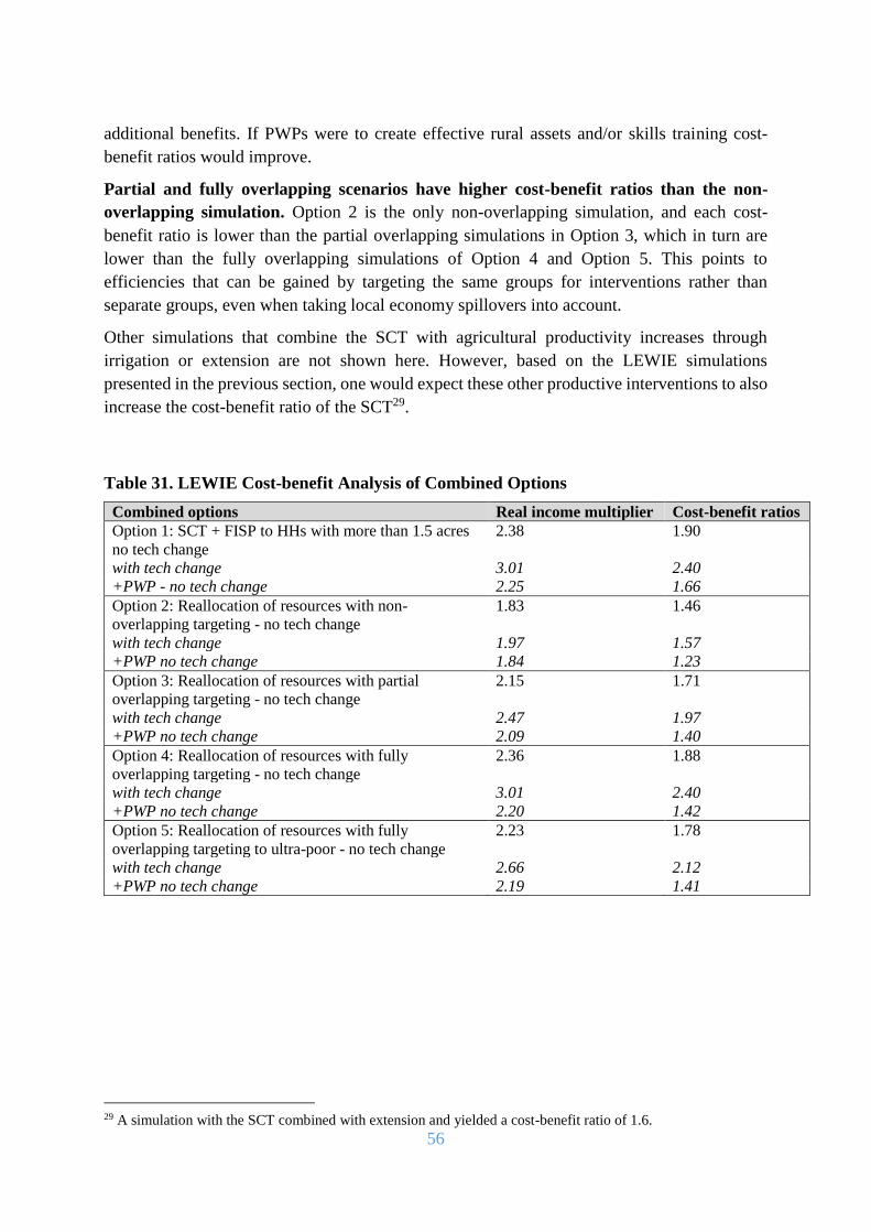
56
additional benefits. If PWPs were to create effective rural assets and/or skills training cost-
benefit ratios would improve.
Partial and fully overlapping scenarios have higher cost-benefit ratios than the non-
overlapping simulation. Option 2 is the only non-overlapping simulation, and each cost-
benefit ratio is lower than the partial overlapping simulations in Option 3, which in turn are
lower than the fully overlapping simulations of Option 4 and Option 5. This points to
efficiencies that can be gained by targeting the same groups for interventions rather than
separate groups, even when taking local economy spillovers into account.
Other simulations that combine the SCT with agricultural productivity increases through
irrigation or extension are not shown here. However, based on the LEWIE simulations
presented in the previous section, one would expect these other productive interventions to also
increase the cost-benefit ratio of the SCT29.
Table 31. LEWIE Cost-benefit Analysis of Combined Options
Combined options Real income multiplier Cost-benefit ratios
Option 1: SCT + FISP to HHs with more than 1.5 acres
no tech change
2.38 1.90
with tech change 3.01 2.40
+PWP - no tech change 2.25 1.66
Option 2: Reallocation of resources with non-
overlapping targeting - no tech change
1.83 1.46
with tech change 1.97 1.57
+PWP no tech change 1.84 1.23
Option 3: Reallocation of resources with partial
overlapping targeting - no tech change
2.15 1.71
with tech change 2.47 1.97
+PWP no tech change 2.09 1.40
Option 4: Reallocation of resources with fully
overlapping targeting - no tech change
2.36 1.88
with tech change 3.01 2.40
+PWP no tech change 2.20 1.42
Option 5: Reallocation of resources with fully
overlapping targeting to ultra-poor - no tech change
2.23 1.78
with tech change 2.66 2.12
+PWP no tech change 2.19 1.41
29 A simulation with the SCT combined with extension and yielded a cost-benefit ratio of 1.6.

57
9. Conclusion
There are inherent policy tradeoffs between the goals of raising agricultural productivity
and achieving social protection of the Malawi’s poor and vulnerable households. The study
shows that the SCT has the largest direct impact on incomes and poverty amongst targeted
ultra-poor and labour-constrained households, while the FISP, PWPs, irrigation and, to a
smaller degree, extension services have larger impacts on agricultural production.
However, the simulations further reveal that there are important synergies between
productive agricultural programmes and social protection. Interventions that raise
agricultural productivity are found to lower food costs, and this has positive real-income effects
for poor households. Conversely, the SCT, which increases food demand create new markets
for food production. If the policy goal is to raise rural incomes and also increase crop
production, the study finds that combining social protection and productive agricultural
interventions is a more effective strategy than doing either one of these alone.
The economy-wide impact evaluations and cost-benefit analyses show that all selected
programmes have direct impacts on beneficiary households and can also generate positive
or negative income and production spillovers affecting non-targeted household groups.
Programmes can create positive income and production spillovers if they raise the demand for
goods and services, creating income generating opportunities for non-beneficiaries engaged in
the production of those goods and services. However, they can also create negative spillovers,
for example, by pushing up the prices of food and raising costs for food consumers, or by
depressing prices for food producers.
In most cases, spillovers result in large positive indirect impacts on incomes of non-
beneficiaries in rural Malawi and create considerable income multipliers. In most cases,
each MK invested in the programmes studied increases income in rural Malawi by more than 1
MK. For example, each MK transferred through the SCT increases total real income by 1.88
MK - that is, by the MK transferred plus an additional 0.88 MK of income spillover. Impact
evaluations that do not consider income and production spillovers miss many, and in some cases
most of the benefits created by these programmes.
Income spillovers from social protection and agricultural interventions have important
implications for equity, as some household groups are in a better position to benefit from
income spillovers, whatever their cause. For example, non-poor households benefit
significantly from the SCT - even though the transfers go only to ultra-poor households. So do
moderately-poor labour-constrained households with land. These ineligible groups benefit from
the transfers as they have the resources to expand production in response to rising local demand,
thus capturing positive income and production spillovers. Asset-poor households do not have
this capacity to respond and income gains of such households depend mostly upon whether or
not they are direct beneficiaries of the SCT, highlighting the need to ensure that the most poor
are benefiting directly from transfers.
Income spillovers are an important part of cost-benefit analyses and strengthen the
argument of the effectiveness of social protection and productive interventions by

58
capturing the full impact of interventions in rural economies. The study demonstrates that
for all SCT options, income spillovers tip the cost-benefit scale in favor of SCT programmes,
as total discounted benefits, including spillovers, always exceed programme costs, including
administrative costs. The same is true for nearly all productive interventions, as well as for all
considered combined social protection plus productive interventions.
Ignoring production and income spillovers not only misses programme benefits, it also
creates the risk of missing negative indirect impacts that could be avoided with well-
designed complementary policies. For instance, if the FISP raises the market supply of food
crops and pushes down food prices, any food producer who does not receive the FISP subsidies
could suffer. Also, the FISP could be regressive if it does not lower food costs, or if it is not
combined with cash transfers to poor farm households. In fact, the study finds that the FISP
reduces income in some household groups that do not receive the subsidies. Policies that
increase local demand or connect producers with outside markets could alleviate this. Similarly,
if the SCT pushes up food prices by raising the demand for food, any household that does not
receive the SCT could suffer. The study finds that the SCT increases income for all household
groups, but some groups benefit far less from spillovers than others. Asset-poor households that
do not receive the transfer and have limited capacities to expand production are found to benefit
the least. Again, policies that simulate local production or connect consumers with outside
markets could alleviate this.
For PWPs and the FISP, benefits depend critically on whether or not they have productive
impacts beyond the immediate direct impacts. For example, the FISP makes inputs cheaper,
thus stimulating input use, but increased use of fertilizer and other inputs may not be enough to
justify programme costs. Likewise, PWPs are inefficient cash transfers if they do not lead to
the creation of productive rural assets and improve productivity through transfers of skills. The
simulations show that the FISP does not pass the cost-benefit test (having ratio of benefits to
costs of larger than 1) if it does not lead to technological change - that is, if it does not make
farmers more productive.
Directing the FISP towards households with some land could improve the productivity of
the subsidy but risks creating negative impacts on poor farming households that are
excluded from the FISP. The FISP can be regressive if it does not lower food prices, or if it is
not combined with cash transfers to poor farming households, which do not receive the subsidy.
Should the Government decide to reform the FISP, it should be directed to households with
land above the median, while those who no longer receive the FISP should be supported with
the SCT. This should create larger productive effects while limiting the adverse consequences
on the real incomes of former FISP beneficiaries. The resulting SCT targeted toward the poorer
households should have a greater impact on poverty. Still, careful attention should be paid to
the marginal farm household with low amounts of land who lose the FISP and may also be
impacted by the negative price effects from increased production by farmers with land above
1.5 acres that receive the FISP.

59
While irrigation and extension interventions do not directly target the most poor, they
nonetheless have significant impacts on income, food prices and poverty. The study
simulates the impacts of scaled-up irrigation and extension services on households with land
above the median (1.5 acres) and finds that in addition to creating direct impacts on beneficiary
households, such productive agricultural interventions have significant impacts on (ultra-
)poverty levels, primarily due to lower food prices resulting from more substantive harvests.
Reducing poverty is the single most important goal of rural development programmes
and social and productive interventions can directly reduce poverty by targeting poor
households as well as indirectly by creating real-income spillovers. The simulation confirms
that social protection interventions, the SCT and PWPs, are cost-effective (benefits exceeding
costs) and have stronger direct and indirect impacts on poverty reduction than any of the
productive programmes studied.
Nevertheless, the largest decrease in poverty results from combined interventions that
target ultra-poor households with the SCT, while raising crop productivity, thus reducing
food prices. Increasing crop productivity can be done through FISP or through other productive
interventions such as irrigation and extension. Even creating effective rural assets with the
PWPs could raise crop productivity and complement the SCT. Lower food prices have a
disproportionately large impact on welfare in poor households, which allocate most of their
budgets to food.
In fact, ensuring overlapping targeting between the SCT and FISP should increase the
cost-effectiveness of both programmes, as partially and fully overlapping policy options
of the SCT and FISP have consistently higher cost-benefit ratios than non-overlapping
options. For the SCT and FISP, non-overlapping policy options have the lowest cost-benefit
ratios and fully overlapping options have consistently the highest ratios. This points to
efficiencies that can be gained by targeting the same groups for interventions rather than
separate groups, even when taking local economy spillovers into account.
Overall, the findings from this study underline the importance of coordinating social
protection with interventions to increase crop productivity. This appears to be critical in
order to create positive real-income multipliers and stimulate agricultural production while
alleviating rural poverty.

60
References
Abdoulayi, S., Angeles, G., Barrington, C., Brugh, K., Handa, S., Hill, M.J., Kilburn, K.,
Otchere, F., Mvula, P., Tsoka, M., and Natali, L. 2014. Malawi Social Cash Transfer
Programme Baseline Evaluation Report. University of North Carolina, Carolina
Population Center (March 29).
Asfaw, S., Cattaneo, A., and Pallante, G. 2016. Welfare and productivity effects of switching
from existing FISP to a universal fertilizer subsidy in Malawi. Rome: Agriculture
Organization of the United Nations (FAO).
Asfaw, S., Pickmans, R., and Davis, B. 2016. Productive impact of Malawi’s Social Cash
Transfer Programme – midterm report. Protection to Production (PtoP) report. Rome:
Agriculture Organization of the United Nations (FAO).
Beegle, K., Galasso, E., and Goldberg, J. 2015. Direct and Indirect Effects of Malawi’s Public
Works Programme on Food Security. Policy Research Working Paper 7505, Washington,
DC: World Bank.
Chafuwa, C. 2017. Priorities for Irrigation Investment in Malawi. Strategy Support
Programme: Policy Note 28. Washington, D.C.: International Food Policy Research
Institute (IFPRI).
Chirwa, E. and Dorward, A. 2013. Targeting in the Farm Input Subsidy Programme in Malawi:
Issues and Options. Working Paper 066, Future Agricultures Consortium.
Daidone, S., Pace, N., Davis, B., Handa, S., Knowles, M., Pickmans, R. 2017. The Social Cash
Transfer Programme and Farm Input Subsidy Programme in Malawi: complementary
instruments for increasing consumption and productive activities. Protection to
Production (PtoP) report. Rome: Agriculture Organization of the United Nations (FAO).
D'Souza, A., Jolliffe, D. 2014. Food Insecurity in Vulnerable Populations: Coping with Food
Price Shocks in Afghanistan. American Journal of Agricultural Economics, 96 (3): 790-
812.
Filipski, M., Taylor, J.E., Thome, K. and Davis, B. Effects of Treatment Beyond the Treated:
A General Equilibrium Impact Evaluation of Lesotho's cash Granst Programme.
Agricultural Economics, 46 (2): 227-243.
Filipski, M., Taylor, J.E., Abegaz, G.A., Ferede, T., Taffesse, A.S., and Diao, X. 2016.
Synopsis: Economy-wide impacts of the Productive Safety Net Programme (PSNP).
ESSP II Research Note 57. Washington, D.C. and Addis Ababa, Ethiopia: International
Food Policy Research Institute (IFPRI) and Ethiopian Development Research Institute
(EDRI). http://ebrary.ifpri.org/cdm/ref/collection/p15738coll2/id/130466
Kagin, J., Taylor, J.E. 2016. Local Economy and Social Capital Impacts of the SCTPP in
Tigray, Ethiopia. Addis Abeba: United Nations Children's Fund.
Kagin, J., Taylor, J.E., Alfani, F., and Davis, B. 2014. Local Economy-wide Impact Evaluation
(LEWIE) of Ethiopia's social cash transfer pilot programme. Protection to Production
(PtoP) report. Rome: Agriculture Organization of the United Nations (FAO).
Logistics Unit, Government of Malawi. 2017. Final Report on the Implementation of the Farm
Input Subsidy Programme (2016-7).

61
Meerendonk, A., Cunha, N., Juegens, F. 2015. Towards a Malawian Social Protection Floor:
Assessment of Social Protection Programmes and Costing of Policy Options.
International Labour Office.
N. Pace, S. Daidone, B. Davis, S. Handa, M. Knowles, R. Pickmans. 2017. One plus one can
be greater than two: evaluating synergies of development Programmes in Malawi.
Journal of Development Studies, 54 (11): 2023-2060.
Pauw, K., and Thurow, J. 2014. Malawi's Farm Input Subsidy Programme: Where Do We Go
From Here? Policy Note 18, Washington, DC: International Food Policy Research
Institute.
PSIConsult. 2017. Consultancy Services for the Development of Agriculture Extension and
Advisory Services Strategy for the Ministry of Agriculture, Irrigation and Water
Development (MOAIWD). Kent: UK. Final Issues Paper.
Ricker‐Gilbert, J., Mason, N.M., Darko, F.A. and Tembo, S.T., 2013. What are the effects of
input subsidy programmes on maize prices? Evidence from Malawi and Zambia.
Agricultural Economics, 44(6), pp.671-686.
Singh, I., Squire, L. and Strauss, J. 1986. Agricultural household models: Extensions,
applications, and policy. The World Bank.
Taylor, J.E., and Filipski, M. 2014. Beyond Experiments in Development Economics: Local
Economy-wide Impact Evaluation. Oxford: Oxford University Press.
Taylor, J.E., Filipski, M., Alloush, M., Gupta, A., Rojas Valdes, R.I., and Gonzalez-Estrada, E.
2016. Economic impact of refugees. Proceedings of the National Academy of Sciences
Taylor, J.E., Gupta, A., Davis, B., Pellerano, L., and Niang, O. 2016. Long-term Impacts of
SCTs: A Local-economy Cost-benefit Analysis. UN FAO and UC Davis, March 19,
2016.
The Agriculture Sector Wide Approach (ASWAp): Malawi's prioritized and harmonized
Agricultural Development Agenda: 2010-2014. Review of Achievements and
Implementation Draft Final Report. Rome: United Nations Food and Agriculture
Organization, 2016.
Thome, K., Taylor, J.E., Tsoka, M., Mvula, P., Davis, B., and Handa, S. 2015. Local Economy-
wide Impact Evaluation (LEWIE) of Malawi's Social Cash Transfer (SCT) Programme.
Protection to Production (PtoP) report. Rome: Agriculture Organization of the United
Nations (FAO).
Thome, K., Taylor, J.E., Kagin, J., Davis, B., Osei, R.D., and Osei-Akoto, I. 2014. Local
Economy-wide Impact Evaluation (LEWIE) of Ghana's Livelihood Empowerment
Against Poverty (LEAP) Programme. Protection to Production (PtoP) report. Rome:
Agriculture Organization of the United Nations (FAO).
Thome, K., Filipski, M., Kagin, J., Taylor, J.E., and Davis, B. 2013. Agricultural Spillover
Effects of Cash Transfers: What Does LEWIE Have to Say. American Journal of
Agricultural Economics, 95 (5): 1338-1344.
University of North Carolina. 2016. Malawi Social Cash Transfer Programme Endline Impact
Evaluation Report. Chapel Hill. University of North Carolina, Chapel Hill, Carolina
Population Center.

62
Appendix A: Impacts on poverty and inequality of
policy options
Table 32 presents the simulated impacts of social protection and agricultural production
interventions on poverty and inequality in rural Malawi. Contrary to typical analyses, the effects
simulated are not only the effects on poverty and inequality of direct transfer effects on
beneficiaries under each policy options. Instead, the distributional implications of the overall
income effects that are driven by spillover production and consumption linkages, including on
non-beneficiary households are simulated.
The top three horizontal panels give impacts of the SCT, PWPs, and FISP. The bottom
horizontal panel presents poverty impacts of the combined interventions. For each policy or
policy combination, the first two columns give the impact on the number of people (headcount)
in moderate poverty; the second two columns, on the number of people in severe (ultra) poverty;
the third two, on the total number of people in poverty; and the last two, on the Gini coefficient
of income inequality. The Gini coefficient ranges from a low of 0 (perfect equity) to a high of
1 (perfect inequality). A decrease in the index indicates lower inequality.
It is clear from both the table and the figures that SCT stand-alone programmes have the
largest impacts on ultra-poverty and inequality of all of the (standalone) interventions we
considered. SCT reduces the total ultra-poverty headcount by 10 percentage points (Option 1)
to 21 percentage points (option 4). The impact on overall poverty reduction are much smaller,
a reflection of the fact that the progamme lifts households of rural ultra-poor into moderate
poverty – hence the increase in moderate poverty rates – but not above the poverty line. Yet,
the SCT has one of the largest impacts on overall poverty, which falls by 1 point (Option 1) to
5 points (Option 5).30 Besides reducing poverty, the SCT also lowers income inequality in rural
Malawi. The Gini coefficient of inequality falls by between 2 and 4 percentage points. These
are considered large decreases in inequality by international standards.
Effects on poverty and inequality reduction are obviously large when the SCT transfer
value is higher (Options 4 and 5), but this also comes with higher programme costs. Targeting
SCT based on poverty or based on labour capacity (the difference between option 4 and 5)
yields similar results in terms of overall poverty and inequality reduction.
PWPs also reduces poverty ranging from 0.3 percentage points (Option 1a) to 5 percentage
points (Option 3a and Option 3b). Its impact on overall poverty is actually larger than its impact
on ultra-poverty when a larger number of paid days is modelled (Option 3a and option 3b). That
is because, unlike the SCT, PWPs does not target the most severely impoverished households
(the ultra-poor) rather those that are moderately poor and ultra-poor with available labour.
PWPs also marginally reduces inequality, but only by 1 percentage point.
FISP has less of an impact on ultra-poverty, a minimal impact on poverty overall and a
possibly negative effect on overall inequality, when ultra-poor “productive” farmers with
30 The overall poverty impact of the SCT is less than it’s ultra-poverty impact because many ultra-poor households
that are targeted “graduate” to become moderately poor but do not exit poverty entirely. This is also why there is
an increase in moderate poverty for the SCT programmes.

63
land are excluded from the programme. Our simulations show that FISP reduces poverty by
1 to 3 percentage points, depending on the option. Most of the FISP options do not affect
inequality at all. One (Option 3 with technological change) reduces it by 1 point, and two others
(and option 4 with and without technological change) increases inequality by 1 point.
Irrigation and extension do not target the poorest rural households, those with land below
the median, and yet in the case of irrigation, it the model predicts a significant impact on
ultra-poverty. Irrigation reduces ultra-poverty by 5 percentage points under the full cost
simulation and 9 percentage points under the annual cost simulation; primarily due to lower
food prices resulting from bigger harvests. Irrigation also produces the largest reductions in the
overall headcount (6 percentage point), however associated with highest interventions costs as
well. Irrigation, has a marginal effect on inequality, reduces inequality by 1 point. Extension
has no effect on inequality and a relatively small effect on poverty reduction.
Table 32. Moderate, Ultra, Overall Poverty Headcount, and Inequality Level and
Percentage Point Changes for Each Programme (Appendix)
Moderate poverty Ultra poverty Overall poverty Inequality
Headcount PP
Change Headcount
PP
Change Headcount
PP
Change Gini
Change
in Gini
Baseline 26% - 37% - 63% - 0.47 - SC
T
Option 1 35% 9 27% -10 62% -1 0.45 -0.02
Option 2 41% 15 20% -17 61% -2 0.43 -0.03
Option 3 32% 6 26% -11 58% -4 0.45 -0.02
Option 4 43% 17 15% -21 59% -4 0.42 -0.04
Option 5 37% 11 21% -16 57% -5 0.43 -0.04 PW
P
Option 1a 26% 0 35% -2 60% -2 0.46 -0.01
Option 1b 26% 0 34% -3 60% -3 0.46 -0.01
Option 2a 29% 3 34% -3 62% 0 0.46 -0.01
Option 2b 29% 3 33% -4 62% -1 0.46 -0.01
Option 3a 25% -1 33% -4 58% -5 0.46 -0.01
Option 3b 25% -1 33% -4 57% -5 0.46 -0.01 FIS
P
Option 1 no tech change 26% 0 36% -1 62% -1 0.47 0.00
Option 1 with tech change 26% 0 35% -2 61% -2 0.47 0.00
Option 2 no tech change 27% -1 34% -1 61% -1 0.47 0.00
Option 2 with tech change 28% -1 32% -2 60% -2 0.46 0.00
Option 3 no tech change 26% -1 35% -3 61% -2 0.46 0.00
Option 3 with tech change 26% -1 33% -5 59% -3 0.46 -0.01
Option 4 no tech change 24% -1 37% 0 61% -1 0.47 0.01
Option 4 with tech change 24% -2 37% 0 61% -2 0.48 0.01
Option 5 no tech change 25% -1 37% 0 62% -1 0.47 0.00
Option 5 with tech change 25% -1 37% 0 62% -1 0.47 0.00 IR Double access to irrigation, full
cost 28% 0 32% -5 60% -1 0.46 0.00
Double access to irrigation,
annual cost 30% 0 28% -9 57% 0 0.46 -0.01
E S Double access to extension 27% 0 35% -2 62% 0 0.47 0.00 C
OM
BIN
ED
Option 1 36% 9 24% -13 60% -2 0.44 -0.02
Option 1 with tech change 36% 9 23% -14 59% -3 0.44 -0.03
Option 1 +PWP - no tech change 35% 8 23% -14 58% -4 0.44 -0.03
Option 2 42% 16 16% -21 57% -5 0.43 -0.04
Option 2 with tech change 41% 15 16% -21 57% -6 0.43 -0.04
Option 2 +PWP - no tech change 40% 14 15% -22 55% -8 0.43 -0.04
Option 3 32% 16 25% -5 56% -6 0.44 -0.03
Option 3 with tech change 32% 15 23% -6 55% -7 0.44 -0.03
Option 3 +PWP - no tech change 31% 14 23% -7 54% -8 0.44 -0.03
Option 4 25% 16 31% 0 56% 0 0.46 -0.01

64
Option 4 with tech change 25% 15 30% 0 55% 0 0.45 -0.01
Option 4 +PWP - no tech change 24% 14 30% 0 54% 0 0.45 -0.02
Option 5 23% 5 32% -5 55% -6 0.46 -0.01
Option 5 with tech change 23% 5 31% -6 54% -7 0.45 -0.02
Option 5 +PWP - no tech change 23% 5 30% -7 53% -8 0.45 -0.02
The largest impacts on poverty occurs with combined options, when SCT id delivered in
combination with FISP and PWPs. As previously discussed demand and production side
interventions have mutually reinforcing effects on income multipliers, hence on poverty. The
total poverty headcount falls by 3 percentage points to 8 percentage points in combined
simulations, and ultra-poverty drops by 6 to 22 percentage points.
The largest impact on ultra-poverty and inequality – respectively 22 and 4 percentage points –
occurs under Option 2, with non-overlapping targeting between SCT and FISP (SCT is
targeting the ultra-poor and FISP is targeting moderately poor and non-poor with land above
1.5 acres). The effects on ultra-poverty reduction and inequality are larger than in the case of
the SCT alone (see option 2 SCT), because ultra-poor also indirectly benefit of spillovers
(particularly price reduction) induced by productive interventions (PWPs and FISP) they are
not directly beneficiaries of. The magnitude of the combined effect is also larger than the sum
of the effects of standalone options.
The decreases in ultra-poverty are about half as big under the option 3 (reallocation of resources
with partial overlapping targeting SCT+FISP), but the effect on overall poverty headcount are
higher in this case.
Option 4, fully overlapping SCT+FISP, have large effects on overall poverty reduction. Option
5, on the other hand, is fully overlapping but targets the ultra-poor for SCT+FISP. It has a large
impact on the ultra-poor but not enough to have a large impact on overall poverty – much of
the ultra-poor become moderately poor but not non-poor. If the goal is to reduce not only the
ultra-poor headcount but also the overall headcount, interventions must be targeted to the
moderately poor as well.

65
Figure 5. Percentage Point Reduction in the Ultra-Poverty and Overall Poverty
Headcount due to Policy Options (Appendix)
Notes: SCT, PWPs, FISP and Combined averages are average percentage reduction across all policy options.
-16%
-14%
-12%
-10%
-8%
-6%
-4%
-2%
0%
SCT PWP FISP IR ES COMBINED
% C
han
ge
in H
ead
count
Percent Reduction in the Ultra-Poverty and Overall Poverty Headcount due to Policy
Options
Ultra-Poverty Headcount Overall Poverty Headcount

66
Appendix B: Detailed tables
Table 33. Summary Statistics of Key Variables
A B C D E F G H I J
Non-poor HH
with land >=
1.5 acres
Non-poor HH
with land < 1.5
acres
Moderately poor HH
with unconstrained
labour and land >=
1.5 acres
Moderately poor HH
with constrained
labour and land >= 1.5
acres
Moderately poor
HH with
unconstrained
labour and land <
1.5 acres
Moderately poor HH
with constrained
labour and land <
1.5 acres
Ultrapoor HH with
unconstrained
labour and land >=
1.5 acres
Ultrapoor HH
with
unconstrained
labour and land
< 1.5 acres
Ultrapoor HH with
constrained
labour and land
>= 1.5 acres
Ultrapoor HH
with
constrained
labour and
land < 1.5
acres
Socio-demographics
HH size 4.28 3.33 4.87 6.04 4.04 4.83 5.42 4.68 6.70 5.56
Percent of total rural households 17% 30% 4% 3% 8% 9% 6% 11% 5% 7%
Percent of HH where the head attended school 25% 31% 19% 16% 20% 15% 11% 16% 7% 12%
Percent of HH that are female headed 23% 30% 12% 30% 18% 49% 14% 18% 30% 50%
Percent of HH where the head is unfit SHWR and/or
chronically ill 10% 12% 3% 21% 3% 28% 2% 2% 14% 18%
Percent of HH that are child (<15) headed 0% 1% 0% 0% 0% 2% 0% 0% 0% 1%
Percent of HH that are elderly (>=65) headed 16% 15% 5% 27% 3% 30% 5% 4% 23% 26%
Dependency ratio 2.62 2.36 2.29 4.17 2.19 4.00 2.43 2.38 4.37 4.23
Crops
Total value of crop harvest 142,725 68,618 136,109 139,210 61,779 62,096 95,129 47,521 97,174 49,396
Yields (output value per acre) 57,859 76,644 55,262 53,849 69,377 68,890 40,695 54,663 40,849 57,578
Total value of maize harvest 62,689 34,556 57,468 57,565 31,344 31,571 45,149 27,574 46,673 23,958
Land owned in acres 3.26 1.10 2.81 3.53 1.00 1.12 2.80 0.98 2.82 1.02
Land cultivated in acres 2.50 0.93 2.50 2.63 0.92 0.97 2.40 0.94 2.44 0.94
Number of hired labor days for crop production 1.76 0.91 0.90 1.08 0.53 0.78 0.47 0.19 0.37 0.25
HH labor days in crop production 159 81 174 179 93 101 175 91 176 102
Total costs of seeds, fertilizer and pesticides 36,054 20,272 31,785 31,946 17,858 19,262 23,245 14,572 23,981 13,738
HH size 4.00 3.14 4.72 5.69 3.99 4.86 5.37 4.74 6.55 5.57
Percent of land that is of good soil quality 50% 39% 45% 44% 39% 45% 40% 34% 43% 39%
Percent of land that is on flat land 54% 45% 57% 57% 55% 55% 67% 58% 66% 60%
Percent of land that has no erosion 59% 52% 64% 58% 60% 60% 73% 66% 68% 65%
Percent of land that is irrigated 15% 11% 15% 15% 13% 12% 14% 12% 14% 14%
Percent of households that had a visit or visited gov.
extension services 5% 3% 5% 8% 6% 4% 6% 3% 6% 4%
Percent of households that harvested crops in the dry
season as well as the rainy season 14% 10% 18% 16% 9% 8% 14% 6% 14% 8%
Percent of households who harvested pemanent crops 41% 38% 34% 39% 35% 38% 29% 26% 36% 37%
Livestock
Value of livestock owned now and livestock byproducts
produced in the last 12 months 267,216 45,530 93,609 26,312 210,068 75,429 61,837 15,471 98,410 22,540
Value of livestock owned 12 months ago and livestock
assets 217,705 34,340 85,585 22,824 165,920 72,482 54,548 14,869 97,100 22,471
HH expenditures on hired labor for livestock 1,905 127 526 23 305 5 127 6 361 33
Purchased inputs for livestock: feed, vet and medicine
costs, livestock equipment 3,167 812 414 366 728 105 204 123 608 358
Household Enterprise
HH annual own business sales 176,946 329,225 66,197 41,427 59,407 65,659 25,109 27,495 35,788 25,781
HH annual own business days of family labor 45.91 35.14 23.62 24.91 27.46 32.87 15.40 13.27 12.99 11.44
HH annual own business days of hired labor 8.87 10.55 6.01 0.75 1.47 1.43 0.56 1.44 0.97 0.58
HH annual own business expenditures (excl. goods for
resale and hired labor) 54,649 86,515 10,334 10,242 17,716 19,850 5,369 3,817 7,043 7,020
HH annual own business profits 65,493 151,708 28,217 18,226 24,174 28,632 11,556 11,381 20,972 13,207
HH annual own business expenditures on goods for
resale (MWK) 122,822 207,814 33,107 14,416 30,981 26,970 4,552 14,271 8,743 8,058
Expenditures
HH annual expenditures on own/received as gifts crops 400,783 289,313 167,708 204,256 116,878 167,341 101,840 85,766 130,639 97,303
HH annual expenditures on own/received as gifts meat
and livestock byproducts 51,918 45,035 22,239 36,786 13,891 22,609 7,420 2,858 9,619 4,582
HH annual expenditures on food from retail stores and
traders 308,290 304,370 149,829 172,775 152,870 147,566 97,456 89,155 102,130 97,517
HH annual expenditures on non-food from retail stores
and traders 84,878 83,254 41,626 51,615 35,045 40,508 25,585 23,672 31,785 26,636
HH annual expenditures from services 66,826 58,683 17,463 23,232 10,991 15,798 3,806 4,101 5,907 5,234
HH annual expenditures from production goods 32,800 27,744 13,983 20,176 12,293 13,588 5,358 3,569 7,859 6,510
HH annual expenditures on goods and services from
outside the local economy 84,450 49,050 21,165 25,513 14,240 23,422 8,339 6,293 12,346 7,910
HH annual expenditures on food 787,094 658,818 352,185 433,464 293,401 350,364 211,723 180,881 249,983 205,462
HH annual expenditures 1,029,945 857,447 434,014 534,353 356,207 430,831 249,805 215,415 300,283 245,691
Income
HH annual income from remittances 27,271 16,565 6,975 17,146 5,180 12,654 3,655 1,411 7,721 9,963
HH annual labor income 76,120 170,373 63,391 46,459 87,404 76,185 74,030 67,371 49,294 58,052
HH annual income 962,455 1,194,584 627,862 670,878 492,604 482,230 512,174 343,268 466,474 351,133
Notes: All values are in 2016 MK yearly averages
Descriptive Statistics

67
Table 34. Local and Outside Input Linkages, by Sector and Household Group
Unconstrained
Labour
Constrained
Labour
Unconstrained
Labour
Constrained
Labour
1.5 acres or
more< 1.5 acres
Land >= 1.5
acres
Constrained
labour and
land >= 1.5
acres
Unconstrained
labour and
land < 1.5
acres
Constrained
labour and
land < 1.5
acres
Land >=
1.5 acres
Land < 1.5
acres
Land >=
1.5 acres
Land < 1.5
acres
A B C D E F G H I J
Total Value-added 10501.12 6855.07 2441.58 8710.03 1904.46 2425.76 3105.05 2970.58 3026.78 1865.02
OUTSIDE 1192.47 778.44 277.26 1078.16 216.26 275.46 251.56 260.96 245.22 151.10
Total Value-added 25003.12 10829.73 2635.46 16375.86 1923.97 5868.60 3661.96 2918.79 4882.72 2337.11
OUTSIDE 1369.02 592.97 144.30 896.64 105.34 321.33 353.34 281.64 471.14 225.51
Total Value-added 2593.33 9229.34 284.39 459.41 279.49 451.80 77.5228 377.2729 121.7633 175.07
OUTSIDE 2.15 1.13 1.37 1.98 3.15 2.71 1.30 2.19 2.09 1.70
crop 0.01 0.01 0.01 0.01 0.02 0.01 0.01 0.01 0.01 0.01
live 0.19 0.10 0.12 0.17 0.28 0.24 0.11 0.19 0.18 0.15
ser 0.16 0.08 0.10 0.14 0.23 0.20 0.09 0.16 0.15 0.12
ret 0.16 0.08 0.10 0.15 0.23 0.20 0.10 0.16 0.15 0.12
Local 0.51 0.27 0.33 0.47 0.75 0.65 0.31 0.52 0.50 0.41
Total Value-added 377.88 673.77 14.10 72.22 184.64 36.08 27.27 69.77 36.51 48.17
OUTSIDE 0.95 1.04 0.81 0.15 0.29 0.28 0.85 0.44 0.36 0.21
crop 0.00 0.00 0.00 0.00 0.00 0.00 0.00 0.00 0.00 0.00
live 0.01 0.01 0.01 0.00 0.00 0.00 0.01 0.01 0.00 0.00
prod 0.00 0.00 0.00 0.00 0.00 0.00 0.00 0.00 0.00 0.00
ser 0.13 0.14 0.11 0.02 0.04 0.04 0.11 0.06 0.05 0.03
ret 0.02 0.02 0.02 0.00 0.01 0.01 0.02 0.01 0.01 0.00
Local 0.16 0.18 0.14 0.03 0.05 0.05 0.14 0.08 0.06 0.04
Total Value-added 1415.18 3708.49 108.84 629.27 132.41 400.28 177.64 116.48 385.58 172.51
OUTSIDE 1.11 0.62 1.27 0.66 1.38 0.65 0.50 1.47 0.20 0.57
crop 0.00 0.00 0.00 0.00 0.00 0.00 0.00 0.00 0.00 0.00
prod 0.06 0.03 0.07 0.04 0.07 0.03 0.03 0.08 0.01 0.03
ser 0.03 0.02 0.04 0.02 0.04 0.02 0.02 0.04 0.01 0.02
ret 0.10 0.05 0.11 0.06 0.12 0.06 0.04 0.13 0.02 0.05
Local 0.19 0.11 0.22 0.11 0.24 0.11 0.09 0.25 0.03 0.10
Crops
Livestock
Retail
Services
Non-agricultural Production
Purchasing/Supplying
Sector
Non-poor Moderately Poor Ultrapoor
Unconstrained Labor Unconstrained Labor Constrained Labor

68
Table 35. Detailed SCT Simulation Multipliers
(1) UP&LC (2)All UP (3) UP, P, & LC(4) UP, higher
amount
(5) UP&LC,
higher amount
Total Income Multiplier
Nominal 2.90 2.99 2.93 3.06 2.96
(CI) ( 2.76- 3.09) ( 2.84- 3.21) ( 2.78- 3.14) ( 2.88- 3.30) ( 2.80- 3.17)
Real 1.88 1.90 1.88 1.91 1.89
(CI) ( 1.80- 1.99) ( 1.81- 2.03) ( 1.79- 2.00) ( 1.81- 2.04) ( 1.80- 2.01)
Total Beneficiary Income Multiplier
Nominal 1.11 1.31 1.46 1.32 1.11
Real 1.03 1.10 1.15 1.09 1.01
Total Non-Beneficiary Income Multiplier
Nominal 1.79 1.69 1.48 1.74 1.85
Real 0.85 0.80 0.73 0.82 0.88
Total Ultra-Poor Income Multiplier
Nominal 1.29 1.31 0.79 1.32 1.30
Real 1.12 1.10 0.62 1.09 1.11
Total Moderately-Poor Income Multiplier
Nominal 0.45 0.48 0.97 0.49 0.47
Real 0.18 0.19 0.67 0.20 0.19
Total Non-Poor Income Multiplier
Nominal 1.15 1.21 1.18 1.25 1.19
Real 0.58 0.60 0.59 0.62 0.60
HH Income Multipliers
A nominal 0.42 0.44 0.42 0.45 0.43
real 0.19 0.20 0.19 0.20 0.19
B nominal 0.74 0.77 0.75 0.80 0.76
real 0.39 0.41 0.40 0.42 0.40
C nominal 0.05 0.06 0.05 0.06 0.05
real 0.02 0.03 0.03 0.03 0.03
D nominal 0.26 0.27 0.41 0.28 0.26
real 0.10 0.11 0.24 0.11 0.10
E nominal 0.06 0.06 0.06 0.07 0.06
real 0.03 0.03 0.03 0.03 0.03
F nominal 0.08 0.09 0.45 0.09 0.08
real 0.03 0.03 0.38 0.03 0.03
G nominal 0.07 0.29 0.08 0.29 0.08
real 0.04 0.24 0.04 0.24 0.04
H nominal 0.11 0.50 0.11 0.50 0.11
real 0.05 0.42 0.05 0.42 0.05
I nominal 0.47 0.23 0.26 0.23 0.47
real 0.43 0.19 0.22 0.19 0.42
J nominal 0.64 0.29 0.34 0.29 0.65
real 0.60 0.25 0.30 0.25 0.59
Production Multipliers
Total 1.94 1.96 1.93 1.98 1.95
Beneficiary Households 0.19 0.56 0.36 0.59 0.20
Non-Beneficiary 1.75 1.41 1.57 1.39 1.75
Ultra-Poor 0.51 0.56 0.53 0.59 0.53
Moderately-Poor 0.25 0.25 0.25 0.24 0.25
Non-Poor 1.18 1.16 1.15 1.14 1.16
Production Multipliers by Sector
crop 0.63 0.67 0.64 0.69 0.65
livestock 0.09 0.09 0.09 0.09 0.09
retail 0.95 0.94 0.93 0.94 0.94
services 0.20 0.18 0.19 0.18 0.20
non-agricultural production 0.07 0.07 0.07 0.07 0.07
Production Multipliers by Sector Beneficiary HHs
crop 0.15 0.46 0.22 0.49 0.17
livestock 0.01 0.02 0.03 0.02 0.01
retail 0.02 0.05 0.07 0.05 0.02
services 0.01 0.02 0.02 0.02 0.01
non-agricultural production 0.00 0.01 0.01 0.01 0.00
Production Multipliers by Sector Non-Beneficiary HHs
crop 0.48 0.21 0.42 0.20 0.48
livestock 0.08 0.07 0.06 0.07 0.08
retail 0.93 0.89 0.86 0.89 0.93
services 0.19 0.17 0.17 0.17 0.19
non-agricultural production 0.07 0.06 0.06 0.06 0.07
Production Multipliers by Sector Ultra-Poor HHs
crop 0.42 0.46 0.44 0.49 0.44
livestock 0.02 0.02 0.02 0.02 0.02
retail 0.05 0.05 0.05 0.05 0.05
services 0.02 0.02 0.02 0.02 0.02
non-agricultural production 0.01 0.01 0.01 0.01 0.01
Production Multipliers by Sector Moderately-Poor HHs
crop 0.08 0.08 0.08 0.08 0.08
livestock 0.03 0.03 0.03 0.03 0.03
retail 0.10 0.09 0.09 0.09 0.10
services 0.04 0.03 0.04 0.03 0.04
non-agricultural production 0.01 0.01 0.01 0.01 0.01
Production Multipliers by Sector Non-Poor HHs
crop 0.13 0.13 0.13 0.12 0.13
livestock 0.04 0.05 0.04 0.04 0.04
retail 0.80 0.80 0.79 0.79 0.80
services 0.14 0.13 0.14 0.13 0.14
non-agricultural production 0.05 0.05 0.05 0.05 0.05
Household
Multipliers
Option
0.00
0.20
0.40
0.60
0.80
1.00
1.20
For all following tables:
Shaded areas are beneficiary
households. A-Non-poor with land >= 1.5 acres, B- Non-poor with land < 1.5 acres, C- Moderately poor with unconstrained
labour and land >= 1.5 acres, D- Moderately poor with constrained
labour and land >= 1.5 acres, E- Moderately poor with unconstrained
labour and land < 1.5 acres, F- Moderately poor with constrained
labour and land < 1.5 acres, G-Ultra-poor HH with unconstrained
labour and land >= 1.5 acres, H-Ultra-poor HH with unconstrained
labour and land < 1.5 acres, I-Ultra-poor HH with constrained
labour and land >= 1.5 acres, J-Ultra-poor HH with constrained
labour and land < 1.5 acres.

69
Table 36. Detailed SCT Simulation Percentages
Percentage Changes (1) UP&LC (2)All UP (3) UP, P, & LC(4) UP, higher
amount
(5) UP&LC,
higher amount
Total Rural Income
Nominal 7.39 17.80 14.76 26.55 16.13
(CI) ( 7.04, 7.86) ( 16.83, 19.10) ( 13.99, 15.81) ( 24.91, 28.65) ( 15.30, 17.26)
Real 5.06 11.57 9.82 16.93 10.82
(CI) ( 4.81, 5.37) ( 10.88, 12.43) ( 9.28, 10.49) ( 15.84, 18.22) ( 10.24, 11.54)
Total Beneficiary Income
Nominal 47.29 52.04 37.57 76.53 101.54
Real 44.11 44.03 31.66 63.23 92.41
Total Non-Beneficiary Income
Nominal 4.38 11.38 9.34 17.17 9.69
Real 2.11 5.47 4.62 8.24 4.67
Total Ultra-Poor Income
Nominal 23.51 52.04 28.40 76.53 50.66
Real 20.84 44.03 22.91 63.23 43.83
Total Moderately-Poor Income
Nominal 3.68 9.58 19.76 14.37 8.08
Real 1.46 3.89 14.70 5.87 3.24
Total Non-Poor Income
Nominal 4.61 12.01 9.54 18.16 10.20
Real 2.31 6.03 4.77 9.07 5.11
Household Income
A nominal 4.03 10.50 8.30 15.77 8.87
real 1.78 4.71 3.69 7.08 3.94
B nominal 4.99 12.99 10.33 19.70 11.07
real 2.66 6.88 5.47 10.36 5.87
C nominal 4.13 10.81 8.51 16.20 9.07
real 1.90 5.07 3.94 7.61 4.20
D nominal 3.82 10.02 12.24 15.00 8.39
real 1.50 4.03 7.28 6.05 3.32
E nominal 3.71 9.56 7.62 14.38 8.18
real 1.60 4.15 3.29 6.27 3.54
F nominal 3.38 8.84 37.46 13.25 7.42
real 1.15 3.12 31.59 4.74 2.56
G nominal 4.90 48.15 10.20 70.88 10.87
real 2.53 39.98 5.27 57.41 5.62
H nominal 4.34 51.00 9.02 74.99 9.63
real 2.14 43.24 4.47 62.15 4.78
I nominal 36.34 44.20 41.46 65.12 78.12
real 33.40 36.63 35.43 52.71 70.06
J nominal 56.46 63.55 61.09 93.30 121.15
real 53.09 54.97 54.23 78.79 111.14
Production by Sector 0.00 0.00 0.00 0.00 0.00
crop 4.39 11.24 8.91 16.56 9.51
livestock 11.92 32.19 9.73 48.97 27.06
retail 3.88 7.57 8.56 10.88 8.33
services 11.73 32.19 24.74 48.97 26.43
non-agricultural production 2.91 7.09 5.75 10.13 6.12
Beneficiary Households Only 3.21 7.84 6.36 11.30 6.78
Production by Sector
crop 5.74 15.36 11.87 22.97 12.64
livestock 2.35 6.04 4.80 8.76 5.02
retail 3.88 9.60 7.75 13.90 8.26
services 3.10 7.24 6.11 10.57 6.64
non-agricultural production 3.93 9.46 7.69 13.87 8.44
Production by Sector Beneficiary HHs
crop 19.69 53.27 13.50 81.99 45.25
livestock 2.72 6.97 4.87 10.19 5.80
retail 5.99 14.87 10.17 21.79 12.89
services 3.10 7.23 6.14 10.64 6.64
non-agricultural production 4.31 10.41 8.03 15.38 9.26
Production by Sector Non-Beneficiary HHs
crop 4.53 5.27 11.07 7.26 9.81
livestock 2.33 5.89 4.76 8.53 4.96
retail 3.86 9.39 7.58 13.58 8.20
services 3.10 7.24 6.10 10.56 6.64
non-agricultural production 3.91 9.38 7.62 13.74 8.39
Ultra-Poor HHs Only
crop 19.10 53.27 40.62 81.99 43.39
livestock 2.70 6.97 5.52 10.19 5.77
retail 5.97 14.87 12.03 21.79 12.83
services 3.11 7.23 6.13 10.64 6.66
non-agricultural production 4.31 10.41 8.45 15.38 9.27
Moderately-Poor HHs Only
crop 2.19 5.28 4.22 7.26 4.46
livestock 2.31 5.89 4.71 8.55 4.93
retail 4.88 12.03 9.79 17.54 10.43
services 3.12 7.28 6.15 10.63 6.68
non-agricultural production 4.05 9.77 7.91 14.36 8.69
Non-Poor HHs Only
crop 2.18 5.26 4.21 7.27 4.45
livestock 2.29 5.89 4.66 8.51 4.87
retail 3.69 9.13 7.36 13.20 7.84
services 3.09 7.22 6.09 10.54 6.62
non-agricultural production 3.87 9.30 7.56 13.62 8.30

70
Table 37. Detailed PWPs Simulation Multipliers
Option 1a (status
quo by end of
2017)
Option 1b (Option
1a with 5% Crop
Land Productivity
Increase)
Option 2a (ultra-
poor labour-
unconstrained
HHs)
Option 2b (Option
2a with 5% Crop
Land Productivity
Increase)
Option 3a (all
poor labour-
unconstrained
HHs with more
days)
Option 3b
(Option 3a with
5% Crop Land
Productivity
Increase)
Nominal 2.87 2.86 2.91 2.90 2.90 2.89
(CI) ( 2.74- 3.05) ( 2.73- 3.04) ( 2.78- 3.09) ( 2.77- 3.09) ( 2.76- 3.09) ( 2.75- 3.08)
Real 1.89 3.24 1.90 3.15 1.89 2.58
(CI) ( 1.80- 1.99) ( 3.16- 3.35) ( 1.82- 2.02) ( 3.07- 3.26) ( 1.80- 2.00) ( 2.50- 2.69)
Total Beneficiary Income Multiplier
Nominal 1.29 1.29 1.18 1.18 1.30 1.29
Real 1.13 1.41 1.08 1.24 1.12 1.27
Total Non-Beneficiary Income Multiplier
Nominal 1.58 1.57 1.73 1.72 1.60 1.60
Real 0.76 1.83 0.82 1.91 0.77 1.31
Total Ultra-Poor Income Multiplier
Nominal 0.88 0.88 1.29 1.29 0.89 0.89
Real 0.73 0.99 1.14 1.38 0.73 0.86
Total Moderately-Poor Income Multiplier
Nominal 0.85 0.85 0.46 0.46 0.86 0.86
Real 0.58 1.02 0.19 0.58 0.58 0.80
Total Non-Poor Income Multiplier
Nominal 1.14 1.13 1.15 1.15 1.15 1.15
Real 0.57 1.24 0.58 1.19 0.58 0.92
HH Income Multipliers
A nominal 0.41 0.41 0.42 0.42 0.42 0.42
real 0.18 0.55 0.19 0.53 0.19 0.37
B nominal 0.72 0.72 0.73 0.73 0.73 0.73
real 0.39 0.69 0.39 0.67 0.39 0.54
C nominal 0.18 0.18 0.05 0.05 0.18 0.18
real 0.15 0.21 0.03 0.07 0.15 0.18
D nominal 0.26 0.25 0.26 0.26 0.26 0.26
real 0.10 0.34 0.11 0.32 0.10 0.22
E nominal 0.33 0.33 0.06 0.06 0.34 0.34
real 0.30 0.36 0.03 0.08 0.29 0.33
F nominal 0.08 0.08 0.08 0.08 0.08 0.08
real 0.03 0.12 0.03 0.11 0.03 0.07
G nominal 0.28 0.28 0.43 0.43 0.28 0.28
real 0.25 0.30 0.39 0.44 0.24 0.28
H nominal 0.49 0.49 0.75 0.75 0.49 0.49
real 0.43 0.54 0.69 0.80 0.43 0.49
I nominal 0.06 0.06 0.06 0.06 0.06 0.06
real 0.03 0.08 0.03 0.07 0.03 0.06
J nominal 0.05 0.05 0.05 0.05 0.05 0.05
real 0.02 0.06 0.02 0.06 0.02 0.04
Production Multipliers
Total 1.94 3.26 1.96 3.17 1.95 2.62
Beneficiary Households 0.41 0.67 0.33 0.48 0.42 0.56
Non-Beneficiary 1.53 2.58 1.63 2.69 1.53 2.06
Ultra-Poor 0.51 0.76 0.52 0.76 0.52 0.66
Moderately-Poor 0.26 0.67 0.26 0.64 0.25 0.46
Non-Poor 1.18 1.83 1.18 1.77 1.17 1.50
Production Multipliers by Sector
crop 0.64 1.96 0.67 1.88 0.65 1.32
livestock 0.09 0.09 0.10 0.10 0.09 0.09
retail 0.95 0.95 0.95 0.96 0.95 0.95
services 0.19 0.19 0.18 0.18 0.19 0.19
non-agricultural production 0.07 0.07 0.07 0.07 0.07 0.07
Production Multipliers by Sector Beneficiary HHs
crop 0.29 0.55 0.27 0.42 0.29 0.43
livestock 0.01 0.01 0.01 0.01 0.01 0.01
retail 0.07 0.07 0.03 0.03 0.07 0.07
services 0.03 0.03 0.01 0.01 0.03 0.03
non-agricultural production 0.00 0.00 0.00 0.00 0.00 0.00
Production Multipliers by Sector Non-Beneficiary HHs
crop 0.36 1.41 0.39 1.45 0.36 0.89
livestock 0.07 0.07 0.08 0.08 0.07 0.07
retail 0.88 0.88 0.92 0.92 0.88 0.88
services 0.16 0.16 0.17 0.17 0.16 0.16
non-agricultural production 0.06 0.06 0.06 0.06 0.06 0.06
Production Multipliers by Sector Ultra-Poor HHs
crop 0.42 0.67 0.43 0.66 0.43 0.56
livestock 0.02 0.02 0.02 0.02 0.02 0.02
retail 0.05 0.05 0.05 0.05 0.05 0.05
services 0.02 0.02 0.02 0.02 0.02 0.02
non-agricultural production 0.01 0.01 0.01 0.01 0.01 0.01
Production Multipliers by Sector Moderately-Poor HHs
crop 0.09 0.50 0.09 0.47 0.09 0.30
livestock 0.03 0.03 0.03 0.03 0.03 0.03
retail 0.10 0.10 0.10 0.10 0.10 0.10
services 0.03 0.03 0.03 0.03 0.03 0.03
non-agricultural production 0.01 0.01 0.01 0.01 0.01 0.01
Production Multipliers by Sector Non-Poor HHs
crop 0.14 0.79 0.14 0.74 0.14 0.46
livestock 0.04 0.04 0.05 0.05 0.04 0.04
retail 0.81 0.81 0.81 0.81 0.80 0.80
services 0.14 0.14 0.13 0.13 0.14 0.14
non-agricultural production 0.05 0.05 0.05 0.05 0.05 0.05
Household
Multipliers
Options
Total Income Multiplier

71
Table 38. Detailed PWPs Simulation Percentages
Percentage Changes
Option 1a (status
quo by end of
2017)
Option 1b (Option
1a with 5% Crop
Land Productivity
Increase)
Option 2a (ultra-
poor labour-
unconstrained
HHs)
Option 2b (Option
2a with 5% Crop
Land Productivity
Increase)
Option 3a (all
poor labour-
unconstrained
HHs with more
days)
Option 3b (Option
3a with 5% Crop
Land Productivity
Increase)
Nominal 3.29 3.28 3.39 3.38 6.64 6.63
(CI) ( 3.14%, 3.50%) ( 3.13%, 3.49%) ( 3.22%, 3.62%) ( 3.21%, 3.61%) ( 6.32%, 7.08%) ( 6.30%, 7.07%)
Real 2.24 3.67 2.22 3.65 4.48 5.94
(CI) ( 2.13%, 2.38%) ( 3.55%, 3.82%) ( 2.10%, 2.38%) ( 3.52%, 3.82%) ( 4.25%, 4.77%) ( 5.70%, 6.24%)
Total Beneficiary Income
Nominal 8.75 8.74 15.33 15.31 17.56 17.55
Real 7.67 9.54 14.01 16.11 15.23 17.23
Total Non-Beneficiary Income
Nominal 2.05 2.04 2.24 2.23 4.16 4.15
Real 1.00 2.33 1.08 2.45 2.03 3.37
Total Ultra-Poor Income
Nominal 6.05 6.04 9.56 9.55 12.17 12.15
Real 4.97 6.81 8.32 10.22 9.90 11.83
Total Moderately-Poor Income
Nominal 4.61 4.60 1.90 1.89 9.26 9.25
Real 3.56 5.28 0.76 2.44 7.09 8.86
Total Non-Poor Income
Nominal 2.13 2.12 2.35 2.34 4.31 4.31
Real 1.07 2.30 1.19 2.41 2.18 3.41
Household Income
A nominal 1.87 1.86 2.08 2.07 3.78 3.77
real 0.83 2.49 0.93 2.59 1.69 3.35
B nominal 2.29 2.29 2.53 2.52 4.66 4.65
real 1.23 2.18 1.35 2.30 2.50 3.45
C nominal 6.67 6.66 2.15 2.14 13.38 13.37
real 5.59 7.53 1.01 2.86 11.12 13.15
D nominal 1.78 1.77 2.00 1.99 3.60 3.58
real 0.71 2.37 0.80 2.46 1.43 3.10
E nominal 9.31 9.30 1.87 1.86 18.66 18.65
real 8.26 9.92 0.80 2.35 16.39 18.18
F nominal 1.57 1.56 1.76 1.75 3.18 3.17
real 0.54 2.24 0.61 2.31 1.09 2.80
G nominal 8.87 8.85 14.60 14.58 17.81 17.79
real 7.71 9.49 13.23 15.10 15.32 17.22
H nominal 9.43 9.42 15.79 15.78 18.93 18.92
real 8.34 10.47 14.50 16.75 16.57 18.86
I nominal 2.20 2.19 2.47 2.45 4.48 4.46
real 1.16 2.83 1.31 2.98 2.37 4.05
J nominal 1.98 1.97 2.22 2.20 4.03 4.02
real 0.95 2.60 1.06 2.72 1.93 3.60
0.00 0.00 0.00 0.00 0.00 0.00
Total Production 2.06 3.80 2.28 4.02 4.14 5.93
Beneficiary Households 3.72 6.08 6.10 8.85 7.55 10.05
Non-Beneficiary Households 1.76 3.38 1.92 3.56 3.53 5.18
Ultra-Poor Households 5.47 8.17 6.15 8.88 11.21 14.15
Moderately-Poor Households 1.38 3.77 1.52 3.92 2.73 5.15
Non-Poor Households 1.51 2.62 1.64 2.75 3.00 4.12
Production by Sector
crop 2.73 7.83 3.08 8.20 5.53 10.77
livestock 1.08 1.07 1.28 1.28 2.15 2.15
retail 1.82 1.83 1.99 2.00 3.64 3.64
services 1.40 1.40 1.41 1.41 2.81 2.80
non-agricultural production 1.76 1.75 1.89 1.88 3.53 3.52
Production by Sector Beneficiary HHs
crop 5.53 10.73 9.94 15.31 11.28 16.76
livestock 1.15 1.15 1.46 1.46 2.31 2.30
retail 2.52 2.53 3.04 3.04 5.05 5.06
services 1.41 1.41 1.42 1.42 2.82 2.82
non-agricultural production 1.89 1.88 2.07 2.07 3.79 3.78
Production by Sector Non-Beneficiary HHs
crop 1.91 6.98 2.05 7.13 3.84 9.01
livestock 1.06 1.06 1.27 1.26 2.13 2.12
retail 1.78 1.78 1.96 1.97 3.55 3.55
services 1.40 1.40 1.41 1.41 2.80 2.80
non-agricultural production 1.75 1.75 1.88 1.88 3.51 3.50
Ultra-Poor HHs Only
crop 8.93 14.26 10.09 15.48 18.37 24.16
livestock 1.23 1.23 1.47 1.47 2.47 2.46
retail 2.79 2.79 3.04 3.05 5.59 5.60
services 1.41 1.40 1.42 1.41 2.82 2.81
non-agricultural production 1.93 1.92 2.07 2.06 3.86 3.86
Moderately-Poor HHs Only
crop 1.08 6.12 1.21 6.26 2.11 7.20
livestock 1.06 1.06 1.26 1.26 2.11 2.11
retail 2.28 2.29 2.49 2.50 4.57 4.57
services 1.41 1.41 1.42 1.42 2.82 2.82
non-agricultural production 1.81 1.80 1.94 1.94 3.63 3.62
Non-Poor HHs Only
crop 1.08 6.12 1.21 6.26 2.11 7.20
livestock 1.05 1.04 1.24 1.24 2.09 2.09
retail 1.74 1.74 1.90 1.90 3.46 3.47
services 1.40 1.40 1.41 1.41 2.80 2.80
non-agricultural production 1.73 1.73 1.86 1.85 3.47 3.46
Total Rural Income

72
Table 39. Detailed FISP Simulation Multipliers
No Tech Change With Tech Change No Tech Change With Tech Change No Tech Change With Tech Change No Tech ChangeWith Tech
ChangeNo Tech Change
With Tech
Change
Nominal -0.04 -0.04 0.18 0.28 0.59 1.10 -0.15 -0.16 -0.11 -0.23
(CI) ( -0.10- 0.03) ( -0.10- 0.03) ( -0.04- 0.42) ( 0.00- 0.66) ( -0.07- 1.66) ( -0.06- 2.81) ( -0.35- 0.02) ( -0.36- 0.01) ( -0.23- 0.02) ( -0.44- 0.00)
Real 1.51 2.49 3.33 5.36 6.03 11.90 1.68 2.84 0.92 2.87
(CI) ( 1.31- 1.87) ( 2.26- 2.85) ( 2.15- 5.06) ( 4.03- 7.64) ( 2.28- 14.78) ( 5.55- 22.80) ( 1.28- 1.99) ( 2.58- 3.20) ( 0.59- 1.18) ( 2.33- 3.43)
Total Beneficiary Income Multiplier
Nominal-0.04 -0.04 0.86 1.33 2.09 4.12 1.10 1.48 0.72 1.91
Real 1.51 2.49 2.67 4.26 3.52 7.03 2.01 3.01 1.22 3.45
Total Non-Beneficiary Income Multiplier
Nominal 0.00 0.00 -0.68 -1.05 -1.49 -3.01 -1.25 -1.64 -0.82 -2.13
Real 0.00 0.00 0.66 1.10 2.51 4.87 -0.33 -0.17 -0.30 -0.58
Total Ultra-Poor Income Multiplier
Nominal 0.03 0.03 0.24 0.34 0.97 1.63 -0.41 -0.47 -0.28 -0.69
Real 0.31 0.49 0.82 1.28 1.99 3.66 -0.09 0.04 -0.10 -0.15
Total Moderately-Poor Income Multiplier
Nominal -0.11 -0.11 -0.28 -0.23 0.70 1.73 -0.28 0.30 -0.16 0.05
Real 0.39 0.71 0.73 1.39 2.47 5.28 0.30 1.28 0.17 1.05
Total Non-Poor Income Multiplier
Nominal 0.04 0.04 0.22 0.17 -1.07 -2.25 0.54 0.01 0.33 0.41
Real 0.81 1.29 1.78 2.69 1.58 2.96 1.47 1.51 0.85 1.98
HH Income Multipliers
A nominal -0.11 -0.11 0.59 0.76 -0.72 -1.45 1.15 0.84 0.72 1.45
real 0.31 0.58 1.47 2.19 0.76 1.45 1.66 1.69 1.01 2.32
B nominal 0.15 0.15 -0.36 -0.58 -0.36 -0.80 -0.61 -0.83 -0.39 -1.04
real 0.50 0.72 0.32 0.50 0.82 1.51 -0.20 -0.18 -0.16 -0.35
C nominal -0.01 -0.01 0.17 0.20 1.02 1.36 0.26 0.12 0.14 0.25
real 0.05 0.09 0.30 0.41 1.24 1.82 0.34 0.23 0.18 0.37
D nominal -0.20 -0.20 -0.23 -0.10 -0.02 0.97 -0.31 0.52 -0.15 0.21
real 0.08 0.25 0.32 0.79 0.94 2.92 0.01 1.08 0.03 0.76
E nominal 0.05 0.05 -0.08 -0.13 -0.11 -0.23 -0.10 -0.14 -0.06 -0.16
real 0.11 0.15 0.05 0.07 0.11 0.21 -0.02 -0.02 -0.02 -0.04
F nominal 0.05 0.05 -0.13 -0.20 -0.18 -0.37 -0.14 -0.20 -0.09 -0.24
real 0.15 0.22 0.07 0.12 0.17 0.33 -0.03 -0.01 -0.02 -0.05
G nominal -0.01 -0.01 0.18 0.25 1.09 1.79 -0.10 -0.11 -0.07 -0.16
real 0.05 0.09 0.31 0.47 1.33 2.29 -0.03 0.00 -0.03 -0.04
H nominal -0.01 -0.01 -0.08 -0.10 -0.10 -0.15 -0.16 -0.19 -0.11 -0.27
real 0.11 0.19 0.16 0.29 0.32 0.69 -0.02 0.03 -0.03 -0.04
I nominal -0.01 -0.01 0.16 0.22 0.00 0.01 -0.08 -0.10 -0.06 -0.14
real 0.05 0.08 0.27 0.41 0.18 0.38 -0.02 0.00 -0.02 -0.04
J nominal 0.05 0.05 -0.03 -0.03 -0.02 -0.03 -0.07 -0.08 -0.05 -0.11
real 0.10 0.13 0.07 0.12 0.14 0.29 -0.01 0.01 -0.02 -0.02
Production Multipliers
Total 1.47 2.47 3.38 5.69 5.96 12.21 1.62 2.87 0.86 2.76
Beneficiary Households 1.47 2.47 6.49 9.94 15.31 28.34 4.67 6.72 2.95 8.06
Non-Beneficiary 0.00 0.00 -3.11 -4.25 -9.35 -16.14 -3.05 -3.86 -2.09 -5.30
Ultra-Poor 0.57 0.76 2.69 4.02 7.90 14.25 -2.22 -2.55 -1.61 -3.87
Moderately-Poor 0.15 0.46 -0.38 0.08 1.53 4.65 0.46 2.57 0.37 2.20
Non-Poor 0.75 1.25 1.07 1.59 -3.47 -6.69 3.37 2.85 2.10 4.43
Production Multipliers by Sector
crop 1.46 2.46 3.33 5.62 5.78 11.89 1.73 3.02 0.94 2.96
livestock 0.00 0.00 0.01 0.02 0.04 0.07 0.00 0.00 0.00 0.00
retail 0.01 0.02 0.03 0.04 0.12 0.22 -0.11 -0.14 -0.07 -0.18
services 0.00 0.00 0.01 0.01 0.01 0.00 0.00 -0.02 0.00 -0.01
non-agricultural production 0.00 0.00 0.01 0.01 0.01 0.02 0.00 -0.01 0.00 -0.01
Production Multipliers by Sector Beneficiary HHs
crop 1.46 2.46 6.47 9.92 15.29 28.31 4.69 6.75 2.96 8.10
livestock 0.00 0.00 0.01 0.01 0.01 0.02 0.00 0.00 0.00 0.00
retail 0.01 0.02 0.01 0.01 0.01 0.01 -0.02 -0.03 -0.01 -0.03
services 0.00 0.00 0.00 0.00 0.00 0.00 0.00 0.00 0.00 0.00
non-agricultural production 0.00 0.00 0.00 0.00 0.00 0.00 0.00 0.00 0.00 0.00
Production Multipliers by Sector Non-Beneficiary HHs
crop 0.00 0.00 -3.14 -4.30 -9.51 -16.41 -2.96 -3.73 -2.03 -5.14
livestock 0.00 0.00 0.00 0.01 0.02 0.05 0.00 0.00 0.00 0.00
retail 0.00 0.00 0.02 0.03 0.11 0.21 -0.09 -0.11 -0.06 -0.14
services 0.00 0.00 0.01 0.00 0.01 0.00 0.00 -0.01 0.00 -0.01
non-agricultural production 0.00 0.00 0.00 0.01 0.01 0.02 0.00 0.00 0.00 -0.01
Production Multipliers by Sector Ultra-Poor HHs
crop 0.57 0.76 2.69 4.02 7.88 14.22 -2.21 -2.54 -1.60 -3.85
livestock 0.00 0.00 0.00 0.00 0.01 0.01 0.00 0.00 0.00 0.00
retail 0.00 0.00 0.00 0.00 0.01 0.01 -0.01 -0.01 0.00 -0.01
services 0.00 0.00 0.00 0.00 0.00 0.00 0.00 0.00 0.00 0.00
non-agricultural production 0.00 0.00 0.00 0.00 0.00 0.00 0.00 0.00 0.00 0.00
Production Multipliers by Sector Moderately-Poor HHs
crop 0.15 0.46 -0.39 0.07 1.51 4.60 0.48 2.58 0.38 2.22
livestock 0.00 0.00 0.00 0.00 0.01 0.02 0.00 0.00 0.00 0.00
retail 0.00 0.00 0.00 0.00 0.01 0.02 -0.01 -0.01 -0.01 -0.02
services 0.00 0.00 0.00 0.00 0.00 0.00 0.00 0.00 0.00 0.00
non-agricultural production 0.00 0.00 0.00 0.00 0.00 0.00 0.00 0.00 0.00 0.00
Production Multipliers by Sector Non-Poor HHs
crop 0.74 1.24 1.03 1.54 -3.61 -6.93 3.47 2.98 2.16 4.60
livestock 0.00 0.00 0.00 0.01 0.02 0.04 0.00 0.00 0.00 0.00
retail 0.01 0.01 0.02 0.03 0.10 0.19 -0.09 -0.12 -0.06 -0.15
services 0.00 0.00 0.01 0.01 0.01 0.00 0.00 -0.01 0.00 -0.01
non-agricultural production 0.00 0.00 0.00 0.01 0.01 0.02 0.00 0.00 0.00 -0.01
Total Income Multiplier
Household
Option 2 - "productive farmers"Option 3 - More vulnerable
"productive" farmers
Option 4 - Less vulnerable
"productive farmers"
Option 5 - Less vulnerable
"productive farmers" and lower Option 1 - Status quo
Multipliers

73
Table 40. Detailed FISP Simulation Percentages
No Tech Change With Tech Change No Tech Change With Tech Change No Tech Change With Tech Change No Tech Change With Tech Change No Tech ChangeWith Tech
Change
Total Rural Income
Nominal 0.19 0.18 0.26 0.19 0.17 0.06 -0.06 -0.34 -0.05 -0.39
(CI) ( -0.08, 0.45) ( -0.08, 0.44) ( -0.54, 1.15) ( -0.91, 1.48) ( -0.49, 0.94) ( -0.90, 1.24) ( -0.70, 0.52) ( -1.08, 0.45) ( -0.27, 0.13) ( -0.67, -0.10)
Real 1.67 2.61 3.34 5.14 1.74 3.16 1.61 2.62 0.53 1.35
(CI) ( 1.31, 2.12) ( 2.24, 3.05) ( 1.95, 5.28) ( 3.48, 7.61) ( 0.54, 4.38) ( 1.10, 6.90) ( 0.96, 2.24) ( 1.91, 3.70) ( 0.26, 0.77) ( 0.95, 1.73)
Total Beneficiary Income
Nominal 0.19 0.18 2.83 3.81 6.13 9.75 4.09 5.38 1.59 3.29
Real 1.67 2.61 6.59 9.92 8.19 13.94 6.13 9.09 2.28 5.41
Total Non-Beneficiary Income
Nominal NA NA -1.37 -2.10 -0.57 -1.14 -2.02 -3.05 -0.83 -2.13
Real NA NA 1.28 2.12 0.95 1.83 -0.53 -0.44 -0.30 -0.57
Total Ultra-Poor Income
Nominal 0.32 0.31 1.51 2.21 1.78 2.99 -2.58 -3.55 -1.12 -2.69
Real 2.19 3.36 5.44 8.57 3.82 7.05 -0.56 0.00 -0.41 -0.58
Total Moderately-Poor Income
Nominal 0.38 0.38 -0.82 -1.32 1.01 1.29 -0.55 -0.88 -0.26 -0.70
Real 2.15 3.27 2.81 4.50 2.91 5.05 1.40 2.59 0.43 1.34
Total Non-Poor Income
Nominal 0.09 0.08 0.32 0.20 -0.54 -1.12 0.75 0.66 0.29 0.30
Real 1.37 2.18 2.98 4.49 0.81 1.51 2.23 3.29 0.80 1.84
Household Income
A nominal -0.46 -0.46 2.45 3.16 -0.88 -1.79 4.47 5.64 1.76 3.48
real 1.27 2.37 6.15 9.15 0.95 1.80 6.49 9.32 2.45 5.58
B nominal 0.44 0.44 -1.07 -1.71 -0.31 -0.69 -1.66 -2.57 -0.67 -1.76
real 1.44 2.06 0.93 1.46 0.72 1.32 -0.54 -0.63 -0.27 -0.58
C nominal -0.27 -0.27 5.68 6.68 9.98 13.34 8.12 10.20 2.77 4.80
real 1.67 2.89 9.96 13.64 12.25 17.98 10.45 14.48 3.54 7.17
D nominal -1.23 -1.24 -1.52 -0.66 -0.05 1.81 -1.85 -0.54 -0.57 0.77
real 0.50 1.59 2.06 5.12 1.79 5.55 0.06 2.89 0.11 2.82
E nominal 1.17 1.17 -2.13 -3.33 -0.87 -1.76 -2.29 -3.64 -0.90 -2.44
real 2.81 3.84 1.17 1.93 0.85 1.61 -0.52 -0.53 -0.28 -0.58
F nominal 0.86 0.86 -2.34 -3.62 -0.97 -1.94 -2.40 -3.80 -0.94 -2.52
real 2.67 3.81 1.29 2.14 0.92 1.76 -0.45 -0.40 -0.25 -0.48
G nominal -0.20 -0.21 5.17 7.25 9.34 15.28 -2.65 -3.61 -1.16 -2.73
real 1.56 2.66 9.01 13.51 11.41 19.55 -0.73 -0.26 -0.48 -0.73
H nominal -0.12 -0.13 -1.39 -1.77 -0.51 -0.75 -2.62 -3.66 -1.14 -2.75
real 1.96 3.28 2.91 5.14 1.72 3.68 -0.38 0.30 -0.34 -0.41
I nominal -0.22 -0.23 5.45 7.52 -0.01 0.11 -2.65 -3.59 -1.16 -2.75
real 1.53 2.63 9.29 13.79 1.86 3.82 -0.75 -0.26 -0.48 -0.76
J nominal 1.84 1.83 -0.97 -1.14 -0.23 -0.34 -2.38 -3.30 -1.03 -2.51
real 3.61 4.73 2.61 4.60 1.62 3.33 -0.48 0.03 -0.36 -0.53
Total Production 1.03 2.20 8.24 13.18 5.01 9.92 1.71 4.06 0.56 2.47
Beneficiary Households 1.03 2.20 19.98 30.53 32.72 61.10 10.95 18.85 4.41 13.11
Non-Beneficiary Households NA NA -6.80 -9.07 -4.33 -7.35 -6.99 -9.86 -3.05 -7.55
Ultra-Poor Households 4.36 6.17 47.05 67.34 35.47 62.41 -20.58 -27.93 -9.26 -22.30
Moderately-Poor Households -0.05 1.54 -2.26 0.92 2.08 7.77 2.01 8.23 1.13 7.68
Non-Poor Households 0.73 1.49 3.49 5.23 -1.64 -3.17 7.60 10.46 2.92 6.32
Production by Sector
crop 4.94 8.44 17.68 28.42 12.86 24.33 3.74 8.35 1.09 4.39
livestock -0.05 -0.05 0.10 0.18 0.12 0.25 -0.05 -0.02 -0.02 0.00
retail 0.02 0.03 0.04 0.07 0.06 0.11 -0.18 -0.26 -0.08 -0.18
services 0.03 0.03 0.06 0.05 0.01 -0.01 0.01 -0.03 0.00 -0.04
non-agricultural production -0.01 -0.02 0.13 0.19 0.08 0.15 -0.10 -0.14 -0.05 -0.10
Production by Sector Beneficiary HHs
crop 4.94 8.44 49.09 74.27 76.13 137.98 30.36 49.92 11.98 33.41
livestock -0.05 -0.05 0.10 0.18 0.11 0.24 -0.05 -0.02 -0.02 0.00
retail 0.02 0.03 0.04 0.06 0.06 0.11 -0.18 -0.25 -0.07 -0.18
services 0.03 0.03 0.06 0.05 0.02 -0.02 0.02 -0.03 0.00 -0.04
non-agricultural production -0.01 -0.02 0.13 0.19 0.09 0.15 -0.10 -0.14 -0.05 -0.10
Production by Sector Non-Beneficiary HHs
crop NA NA -26.39 -35.91 -14.35 -24.54 -20.96 -30.20 -9.01 -22.53
livestock NA NA 0.10 0.18 0.12 0.25 -0.05 -0.02 -0.02 0.00
retail NA NA 0.04 0.07 0.06 0.11 -0.18 -0.26 -0.08 -0.18
services NA NA 0.06 0.05 0.01 -0.01 0.01 -0.03 0.00 -0.04
non-agricultural production NA NA 0.13 0.19 0.08 0.15 -0.10 -0.14 -0.05 -0.11
Ultra-Poor HHs Only
crop 10.23 13.85 74.79 109.37 66.46 117.28 -40.55 -55.18 -18.28 -43.79
livestock -0.06 -0.06 0.11 0.21 0.14 0.29 -0.06 -0.02 -0.02 0.00
retail 0.04 0.04 0.07 0.10 0.09 0.17 -0.27 -0.39 -0.11 -0.27
services 0.03 0.03 0.06 0.05 0.02 -0.01 0.01 -0.03 0.00 -0.04
non-agricultural production -0.01 -0.02 0.14 0.21 0.09 0.17 -0.11 -0.15 -0.05 -0.12
Moderately-Poor HHs Only
crop 1.10 4.49 -2.93 3.08 6.76 18.23 6.83 19.31 3.15 16.15
livestock -0.05 -0.05 0.09 0.18 0.11 0.24 -0.05 -0.02 -0.02 0.00
retail 0.03 0.03 0.06 0.08 0.08 0.14 -0.23 -0.32 -0.09 -0.23
services 0.03 0.03 0.06 0.05 0.01 -0.01 0.02 -0.03 0.00 -0.04
non-agricultural production -0.01 -0.02 0.13 0.19 0.09 0.16 -0.11 -0.15 -0.05 -0.11
Non-Poor HHs Only
crop 5.41 8.93 6.65 9.80 -7.68 -14.72 22.21 29.84 8.63 18.04
livestock -0.05 -0.05 0.10 0.17 0.11 0.24 -0.05 -0.02 -0.02 0.00
retail 0.02 0.03 0.04 0.06 0.06 0.10 -0.17 -0.25 -0.07 -0.17
services 0.03 0.03 0.06 0.05 0.01 -0.01 0.01 -0.03 0.00 -0.04
non-agricultural production -0.01 -0.02 0.13 0.19 0.08 0.15 -0.10 -0.14 -0.05 -0.10
Percentage Changes
Option 2 - "productive farmers"Option 3 - More vulnerable
"productive" farmers
Option 4 - Less vulnerable
"productive farmers"
Option 5 - Less vulnerable
"productive farmers" and lower
subsidy
Option 1 - Status quo

74
Table 41. Detailed Irrigation and Extension Simulation Multipliers
MultipliersIrrigation (Full
Cost)
Irrigation (Annual
Cost)Extension
Total Income Multiplier
Nominal 0.87 0.89 2.63
(CI) ( 0.83- 0.93) ( 0.85- 0.96) ( 2.51- 2.80)
Real 0.85 0.69 2.07
(CI) ( 0.78- 0.96) ( 0.65- 0.76) ( 1.98- 2.24)
Total Beneficiary Income Multiplier
Nominal 0.67 0.62 1.86
Real 0.68 0.53 1.61
Total Non-Beneficiary Income Multiplier
Nominal 0.20 0.27 0.77
Real 0.17 0.16 0.46
Total Ultra-Poor Income Multiplier
Nominal 0.18 0.18 0.53
Real 0.18 0.16 0.46
Total Moderately-Poor Income Multiplier
Nominal 0.21 0.21 0.63
Real 0.22 0.16 0.48
Total Non-Poor Income Multiplier
Nominal 0.48 0.50 1.48
Real 0.45 0.38 1.12
HH Income Multipliers
A nominal 0.32 0.30 0.90
real 0.33 0.25 0.78
B nominal 0.16 0.20 0.58
real 0.12 0.12 0.35
C nominal 0.06 0.05 0.16
real 0.06 0.05 0.15
D nominal 0.14 0.12 0.37
real 0.14 0.10 0.29
E nominal 0.01 0.01 0.04
real 0.01 0.01 0.02
F nominal 0.01 0.02 0.05
real 0.01 0.01 0.03
G nominal 0.09 0.08 0.24
real 0.09 0.07 0.22
H nominal 0.02 0.02 0.07
real 0.02 0.02 0.05
I nominal 0.07 0.06 0.19
real 0.07 0.06 0.17
J nominal 0.01 0.01 0.03
real 0.01 0.01 0.02
Production Multipliers
Total 0.86 0.71 2.10
Beneficiary Households 0.83 0.50 1.45
Non-Beneficiary 0.03 0.21 0.65
Ultra-Poor 0.18 0.17 0.41
Moderately-Poor 0.20 0.13 0.42
Non-Poor 0.48 0.41 1.27
Production Multipliers by Sector
crop 0.47 0.32 0.91
livestock 0.03 0.03 0.09
retail 0.28 0.28 0.86
services 0.06 0.06 0.18
non-agricultural production 0.02 0.02 0.06
Production Multipliers by Sector Beneficiary HHs
crop 0.73 0.40 1.14
livestock 0.02 0.02 0.05
retail 0.06 0.06 0.18
services 0.02 0.02 0.05
non-agricultural production 0.01 0.01 0.02
Production Multipliers by Sector Non-Beneficiary HHs
crop -0.25 -0.08 -0.23
livestock 0.01 0.01 0.04
retail 0.22 0.22 0.68
services 0.04 0.04 0.13
non-agricultural production 0.01 0.01 0.04
Production Multipliers by Sector Ultra-Poor HHs
crop 0.16 0.14 0.32
livestock 0.01 0.01 0.02
retail 0.01 0.02 0.05
services 0.01 0.01 0.02
non-agricultural production 0.00 0.00 0.01
Production Multipliers by Sector Moderately-Poor HHs
crop 0.15 0.08 0.26
livestock 0.01 0.01 0.03
retail 0.03 0.03 0.09
services 0.01 0.01 0.03
non-agricultural production 0.00 0.00 0.01
Production Multipliers by Sector Non-Poor HHs
crop 0.17 0.10 0.33
livestock 0.01 0.01 0.04
retail 0.24 0.24 0.73
services 0.04 0.04 0.13
non-agricultural production 0.02 0.02 0.05

75
Table 42. Detailed Irrigation and Extension Simulation Percentages
Percentage ChangesIrrigation (Full
Cost, annualized)
Irrigation (Annual
Cost)Extension
Total Rural Income
Nominal 6.09 14.66 3.18
(CI) ( 5.65, 6.65) ( 13.75, 15.98) ( 3.01, 3.41)
Real 5.87 11.30 2.48
(CI) ( 5.33, 6.75) ( 10.50, 12.62) ( 2.33, 2.71)
Total Beneficiary Income
Nominal 11.28 24.09 5.33
Real 11.43 20.87 4.69
Total Non-Beneficiary Income
Nominal 2.82 8.71 1.83
Real 2.37 5.27 1.09
Total Ultra-Poor Income
Nominal 8.61 20.44 4.40
Real 8.91 17.46 3.80
Total Moderately-Poor Income
Nominal 4.36 11.20 2.45
Real 4.55 8.43 1.85
Total Non-Poor Income
Nominal 6.06 14.41 3.13
Real 5.57 10.76 2.37
Household Income
A nominal 9.94 21.08 4.69
real 10.08 17.95 4.06
B nominal 3.54 10.08 2.12
real 2.64 6.09 1.27
C nominal 13.87 29.91 6.68
real 14.33 26.94 6.10
D nominal 6.68 13.58 3.01
real 6.72 10.44 2.34
E nominal 1.57 6.36 1.34
real 1.70 3.78 0.77
F nominal 1.16 5.52 1.17
real 1.36 2.86 0.57
G nominal 18.25 39.88 8.70
real 18.30 35.96 7.99
H nominal 2.02 7.39 1.52
real 2.65 5.19 1.02
I nominal 16.95 36.91 8.03
real 17.11 33.39 7.38
J nominal 2.32 7.65 1.58
real 2.45 4.88 0.97
Total Production 9.55 15.58 3.29
Beneficiary Households 18.09 25.05 5.25
Non-Beneficiary Households -1.41 3.44 0.78
Ultra-Poor Households 24.27 42.32 7.56
Moderately-Poor Households 8.84 12.61 2.96
Non-Poor Households 5.93 9.96 2.31
Production by Sector
crop 15.75 24.10 4.89
livestock 2.43 5.43 1.23
retail 3.66 8.40 1.90
services 2.94 6.81 1.53
non-agricultural production 3.64 8.34 1.86
Production by Sector Beneficiary HHs
crop 38.17 49.05 10.09
livestock 2.40 5.35 1.22
retail 3.67 8.43 1.91
services 2.94 6.81 1.53
non-agricultural production 3.69 8.46 1.89
Production by Sector Non-Beneficiary HHs
crop -15.71 -10.92 -2.42
livestock 2.49 5.57 1.26
retail 3.66 8.39 1.90
services 2.94 6.81 1.53
non-agricultural production 3.61 8.29 1.85
Ultra-Poor HHs Only
crop 34.77 63.29 10.77
livestock 2.82 6.32 1.43
retail 5.56 12.92 2.88
services 2.93 6.78 1.52
non-agricultural production 4.05 9.31 2.07
Moderately-Poor HHs Only
crop 13.62 16.67 4.01
livestock 2.35 5.24 1.19
retail 4.59 10.61 2.38
services 2.93 6.78 1.52
non-agricultural production 3.80 8.72 1.95
Non-Poor HHs Only
crop 8.44 11.36 2.79
livestock 2.38 5.30 1.21
retail 3.48 7.98 1.81
services 2.95 6.82 1.53
non-agricultural production 3.56 8.17 1.83

76
Table 43. Detailed Combined Intervention Simulation Multipliers
No Tech Change With Tech ChangeW/ PWP No Tech
ChangeNo Tech Change With Tech Change
W/ PWP No
Tech ChangeNo Tech Change
With Tech
Change
W/ PWP No
Tech ChangeNo Tech Change With Tech Change
W/ PWP No
Tech ChangeNo Tech Change
With Tech
Change
W/ PWP No
Tech Change
Total Income Multiplier
Nominal 2.07 2.10 2.30 2.73 2.71 2.77 2.79 2.82 2.85 2.70 2.74 2.77 2.93 2.98 2.95
(CI) ( 1.92- 2.24) ( 1.93- 2.29) ( 2.13- 2.48) ( 2.57- 2.95) ( 2.55- 2.90) ( 2.61- 3.01) ( 2.62- 3.00) ( 2.61- 3.06) ( 2.67- 3.06) ( 2.54- 2.92) ( 2.55- 2.99) ( 2.59- 2.97) ( 2.77- 3.15) ( 2.78- 3.24) ( 2.76- 3.16)
Real 2.38 3.01 2.25 1.83 1.97 1.84 2.15 2.47 2.09 2.36 3.01 2.20 2.23 2.66 2.19
(CI) ( 1.96- 3.01) ( 2.51- 3.70) ( 1.93- 2.79) ( 1.79- 1.89) ( 1.92- 2.02) ( 1.79- 1.89) ( 1.84- 2.77) ( 2.01- 3.29) ( 1.83- 2.62) ( 1.92- 3.36) ( 2.23- 4.26) ( 1.87- 2.87) ( 2.01- 2.48) ( 2.37- 2.95) ( 1.99- 2.41)
Total Beneficiary Income Multiplier
Nominal 1.60 1.74 1.78 1.96 2.02 2.04 1.61 1.74 1.77 1.49 1.70 1.60 1.35 1.44 1.46
Real 1.85 2.36 1.83 1.45 1.61 1.46 1.4 1.65 1.45 1.42 1.81 1.43 1.23 1.41 1.28
Total Non-Beneficiary Income Multiplier
Nominal 0.47 0.35 0.52 0.76 0.69 0.74 1.18 1.08 1.08 1.22 1.04 1.17 1.58 1.54 1.5
Real 0.53 0.65 0.42 0.39 0.36 0.38 0.75 0.82 0.64 0.94 1.20 0.76 1 1.24 0.9
Total Ultra-Poor Income Multiplier
Nominal 0.98 1.00 0.96 1.13 1.09 1.11 0.81 0.85 0.83 0.79 0.86 0.82 1.35 1.44 1.29
Real 1.07 1.22 0.98 0.96 0.96 0.92 0.72 0.82 0.71 0.76 0.95 0.74 1.23 1.41 1.15
Total Moderately-Poor Income Multiplier
Nominal 0.23 0.24 0.39 0.41 0.42 0.46 0.95 1.02 0.94 0.98 1.08 0.95 0.44 0.42 0.5
Real 0.35 0.55 0.41 0.19 0.25 0.23 0.79 0.95 0.74 0.91 1.22 0.80 0.27 0.36 0.32
Total Non-Poor Income Multiplier
Nominal 0.86 0.86 0.95 1.19 1.20 1.21 1.03 0.95 1.08 0.94 0.80 1.01 1.15 1.13 1.16
Real 0.95 1.24 0.86 0.68 0.77 0.68 0.65 0.71 0.64 0.70 0.85 0.65 0.73 0.88 0.71
HH Income Multipliers
A nominal 0.47 0.54 0.47 0.54 0.60 0.54 0.35 0.31 0.37 0.31 0.23 0.34 0.4 0.38 0.41
real 0.58 0.81 0.49 0.34 0.44 0.33 0.23 0.25 0.22 0.25 0.33 0.23 0.26 0.33 0.25
B nominal 0.39 0.32 0.49 0.65 0.60 0.67 0.68 0.65 0.71 0.63 0.58 0.67 0.75 0.75 0.76
real 0.37 0.43 0.38 0.34 0.33 0.35 0.42 0.45 0.42 0.44 0.52 0.42 0.47 0.55 0.46
C nominal 0.09 0.10 0.11 0.08 0.09 0.09 0.11 0.13 0.12 0.41 0.44 0.35 0.05 0.05 0.07
real 0.11 0.14 0.12 0.06 0.08 0.07 0.09 0.13 0.1 0.41 0.47 0.33 0.04 0.05 0.05
D nominal 0.11 0.14 0.14 0.22 0.23 0.22 0.38 0.45 0.36 0.47 0.57 0.41 0.25 0.24 0.25
real 0.17 0.31 0.15 0.09 0.13 0.09 0.29 0.4 0.25 0.42 0.64 0.33 0.15 0.21 0.15
E nominal 0.02 0.00 0.10 0.05 0.04 0.08 0.05 0.04 0.1 0.04 0.03 0.12 0.06 0.05 0.1
real 0.03 0.04 0.10 0.02 0.02 0.05 0.03 0.04 0.08 0.04 0.05 0.11 0.04 0.05 0.08
F nominal 0.02 -0.01 0.03 0.06 0.05 0.07 0.41 0.4 0.35 0.06 0.04 0.06 0.08 0.07 0.08
real 0.04 0.06 0.04 0.02 0.02 0.02 0.37 0.38 0.31 0.04 0.06 0.04 0.04 0.06 0.04
G nominal 0.11 0.13 0.16 0.25 0.24 0.25 0.15 0.2 0.18 0.61 0.69 0.52 0.3 0.32 0.3
real 0.13 0.17 0.16 0.21 0.21 0.21 0.13 0.19 0.15 0.60 0.71 0.50 0.27 0.31 0.27
H nominal 0.04 0.04 0.15 0.43 0.42 0.44 0.09 0.08 0.16 0.08 0.08 0.19 0.51 0.54 0.51
real 0.08 0.12 0.17 0.37 0.37 0.37 0.07 0.08 0.13 0.08 0.12 0.17 0.47 0.54 0.47
I nominal 0.38 0.40 0.30 0.19 0.19 0.18 0.25 0.24 0.21 0.05 0.06 0.06 0.24 0.26 0.21
real 0.40 0.44 0.31 0.16 0.16 0.15 0.22 0.23 0.19 0.05 0.07 0.04 0.22 0.25 0.19
J nominal 0.44 0.44 0.34 0.25 0.25 0.23 0.32 0.32 0.27 0.04 0.04 0.04 0.29 0.31 0.26
real 0.46 0.48 0.34 0.22 0.22 0.20 0.3 0.31 0.25 0.04 0.05 0.03 0.27 0.3 0.23
Production Multipliers
Total 2.45 3.19 2.33 1.89 2.03 1.90 2.21 2.56 2.15 2.41 3.13 2.25 2.29 2.78 2.26
Beneficiary Households 2.48 3.56 1.87 1.08 1.29 1.12 1.33 1.99 1.22 2.02 3.49 1.45 1.3 2.13 1.27
Non-Beneficiary -0.03 -0.37 0.46 0.81 0.74 0.78 0.88 0.57 0.93 0.39 -0.36 0.80 0.99 0.65 0.99
Ultra-Poor 1.26 1.68 1.06 0.18 -0.05 0.20 1.03 1.33 0.91 1.36 2.11 1.08 1.3 2.13 1.22
Moderately-Poor 0.05 0.19 0.10 0.30 0.44 0.29 0.31 0.54 0.31 0.38 0.69 0.35 0.1 -0.04 0.12
Non-Poor 1.14 1.32 1.16 1.42 1.64 1.40 0.87 0.69 0.93 0.67 0.33 0.83 0.89 0.69 0.92
Production Multipliers by Sector
crop 1.52 2.25 1.31 0.75 0.91 0.75 0.99 1.34 0.92 1.23 1.93 1.04 1.04 1.5 1
livestock 0.06 0.07 0.07 0.08 0.08 0.08 0.09 0.09 0.09 0.09 0.10 0.09 0.09 0.09 0.09
retail 0.67 0.68 0.74 0.83 0.82 0.84 0.89 0.89 0.89 0.86 0.87 0.88 0.92 0.94 0.92
services 0.14 0.14 0.15 0.17 0.17 0.17 0.18 0.18 0.18 0.17 0.17 0.18 0.18 0.18 0.18
non-agricultural production 0.05 0.05 0.06 0.06 0.06 0.06 0.06 0.07 0.07 0.06 0.06 0.06 0.07 0.07 0.07
Production Multipliers by Sector Beneficiary HHs
crop 2.23 3.31 1.52 0.73 0.94 0.73 1.17 1.83 0.98 1.93 3.40 1.28 1.21 2.04 1.12
livestock 0.04 0.04 0.05 0.06 0.06 0.06 0.04 0.04 0.04 0.03 0.03 0.03 0.02 0.02 0.02
retail 0.15 0.15 0.20 0.21 0.21 0.23 0.09 0.09 0.14 0.04 0.04 0.09 0.05 0.05 0.09
services 0.04 0.05 0.07 0.06 0.06 0.08 0.02 0.02 0.05 0.01 0.01 0.04 0.02 0.02 0.04
non-agricultural production 0.02 0.02 0.02 0.02 0.02 0.02 0.01 0.01 0.02 0.01 0.01 0.01 0.01 0.01 0.01
Production Multipliers by Sector Non-Beneficiary HHs
crop -0.71 -1.06 -0.21 0.02 -0.04 0.02 -0.18 -0.49 -0.05 -0.70 -1.47 -0.24 -0.17 -0.54 -0.11
livestock 0.02 0.03 0.02 0.03 0.03 0.03 0.05 0.05 0.04 0.06 0.07 0.06 0.07 0.07 0.07
retail 0.53 0.53 0.53 0.62 0.61 0.60 0.8 0.8 0.76 0.81 0.83 0.79 0.87 0.89 0.83
services 0.09 0.09 0.08 0.11 0.11 0.09 0.16 0.16 0.13 0.16 0.16 0.14 0.16 0.16 0.14
non-agricultural production 0.03 0.03 0.04 0.04 0.04 0.04 0.05 0.05 0.05 0.05 0.06 0.05 0.06 0.06 0.06
Production Multipliers by Sector Ultra-Poor HHs
crop 1.20 1.61 0.99 0.09 -0.13 0.12 0.94 1.24 0.83 1.27 2.02 0.99 1.21 2.04 1.13
livestock 0.01 0.01 0.01 0.02 0.02 0.02 0.02 0.02 0.02 0.02 0.02 0.02 0.02 0.02 0.02
retail 0.04 0.04 0.04 0.05 0.04 0.05 0.05 0.05 0.05 0.05 0.05 0.05 0.05 0.05 0.05
services 0.01 0.01 0.01 0.01 0.01 0.01 0.02 0.02 0.02 0.02 0.02 0.02 0.02 0.02 0.02
non-agricultural production 0.00 0.00 0.00 0.01 0.01 0.01 0.01 0.01 0.01 0.01 0.01 0.01 0.01 0.01 0.01
Production Multipliers by Sector Moderately-Poor HHs
crop -0.07 0.07 -0.03 0.15 0.29 0.14 0.15 0.38 0.15 0.22 0.53 0.19 -0.07 -0.21 -0.05
livestock 0.02 0.02 0.02 0.02 0.03 0.02 0.03 0.03 0.03 0.03 0.03 0.03 0.03 0.03 0.03
retail 0.07 0.07 0.07 0.08 0.08 0.09 0.09 0.09 0.09 0.09 0.08 0.09 0.09 0.09 0.09
services 0.03 0.03 0.03 0.03 0.03 0.03 0.03 0.03 0.03 0.03 0.03 0.03 0.03 0.03 0.03
non-agricultural production 0.01 0.01 0.01 0.01 0.01 0.01 0.01 0.01 0.01 0.01 0.01 0.01 0.01 0.01 0.01
Production Multipliers by Sector Non-Poor HHs
crop 0.39 0.57 0.35 0.51 0.75 0.49 -0.1 -0.28 -0.05 -0.27 -0.62 -0.14 -0.11 -0.33 -0.08
livestock 0.03 0.03 0.03 0.04 0.04 0.04 0.04 0.04 0.04 0.05 0.05 0.04 0.04 0.04 0.04
retail 0.57 0.58 0.62 0.70 0.69 0.70 0.76 0.75 0.76 0.72 0.74 0.74 0.77 0.79 0.78
services 0.10 0.10 0.11 0.12 0.12 0.12 0.13 0.13 0.13 0.12 0.12 0.13 0.13 0.13 0.13
non-agricultural production 0.04 0.04 0.04 0.05 0.05 0.05 0.05 0.05 0.05 0.05 0.05 0.05 0.05 0.05 0.05
HouseholdOption 1: SCT + FISP to HHs with more than 1.5 acres
Option 2: Reallocation of resources with non-
overlapping targeting
Option 3: Reallocation of resources with partial
overlapping targeting
Option 4: Reallocation of resources with fully
overlapping targeting
Option 5: Reallocation of resources with fully
overlapping targeting to ultra-poor
Multipliers

77
Table 44. Detailed Combined Intervention Simulation Percentages
No Tech Change With Tech ChangeW/ PWP No Tech
ChangeNo Tech Change With Tech Change
W/ PWP No Tech
ChangeNo Tech Change With Tech Change
W/ PWP No Tech
ChangeNo Tech Change With Tech Change
W/ PWP No Tech
ChangeNo Tech Change With Tech Change
W/ PWP No Tech
Change
Total Rural Income
Nominal 7.62 7.54 11.05 26.32 25.92 29.99 14.88 14.73 18.45 7.57 7.40 10.95 18.29 18.66 21.84
(CI) ( 6.59%, 8.82%) ( 6.25%, 9.12%) ( 9.86%, 12.51%) ( 24.60%, 28.86%) ( 24.15%, 27.98%)( 28.01%, 32.80%)( 13.62%, 16.49%)( 13.08%, 16.82%)( 16.85%, 20.52%) ( 6.66%, 8.67%) ( 6.20%, 8.91%) ( 9.78%, 12.44%) ( 17.09%, 19.93%)( 17.14%, 20.84%)( 20.19%, 23.77%)
Real 8.59 10.47 10.82 18.04 19.02 20.24 11.71 12.97 13.85 6.56 8.13 8.65 14.05 16.64 16.37
(CI) ( 7.00%, 11.09%) ( 8.52%, 13.30%) ( 9.11%, 13.38%) ( 17.06%, 19.34%) ( 17.95%, 20.21%)( 19.15%, 21.73%)( 10.04%, 14.89%)( 10.51%, 17.24%)( 12.16%, 17.19%) ( 5.13%, 9.59%) ( 5.62%, 12.07%) ( 7.27%, 11.54%) ( 12.53%, 15.85%)( 14.57%, 19.02%)( 14.70%, 18.31%)
Total Beneficiary Income
Nominal 13.83 14.74 15.69 37.65 38.54 39.34 27.51 28.40 30.19 32.48 36.28 17.45 56.08 59.85 45.61
Real 15.49 18.89 16.15 28.97 31.58 29.30 24.41 27.15 25.62 31.64 38.09 15.42 51.24 58.68 39.87
Total Non-Beneficiary Income
Nominal 3.04 2.21 5.60 15.91 14.32 19.00 8.83 8.19 11.32 4.50 3.83 7.02 11.20 10.93 13.68
Real 3.49 4.24 4.54 8.00 7.48 9.59 5.63 6.18 6.70 3.47 4.43 4.54 7.07 8.74 8.30
Total Ultra-Poor Income
Nominal 25.15 25.70 31.28 72.73 70.23 79.01 30.36 31.52 36.67 14.85 16.15 20.98 56.08 59.85 62.63
Real 27.20 30.64 31.96 61.88 61.80 66.11 27.28 30.45 31.88 14.24 17.89 18.92 51.24 58.68 56.14
Total Moderately-Poor Income
Nominal 2.81 2.19 7.47 13.86 13.43 18.67 20.70 21.03 25.52 10.26 10.46 14.90 9.03 8.49 13.78
Real 4.36 5.96 7.90 6.77 7.79 10.19 17.81 19.91 21.11 9.62 11.95 12.91 5.61 7.50 9.21
Total Non-Poor Income
Nominal 4.87 4.81 7.18 18.93 19.07 21.54 8.90 8.24 11.32 4.78 4.09 7.02 11.96 11.79 14.32
Real 5.35 6.94 6.47 10.88 12.12 12.14 5.60 6.08 6.70 3.54 4.31 4.54 7.59 9.18 8.79
Household Income
A nominal 6.50 7.40 8.59 20.82 23.39 23.26 7.34 6.34 9.42 3.77 2.77 5.75 9.99 9.45 12.01
real 8.02 11.23 8.92 13.18 17.12 14.31 4.69 5.25 5.48 3.10 4.06 3.83 6.44 8.32 7.40
B nominal 3.82 3.12 6.26 17.70 16.26 20.42 9.91 9.48 12.56 5.43 4.95 7.84 13.24 13.31 15.82
real 3.62 4.15 4.88 9.38 8.87 10.73 6.19 6.62 7.50 3.82 4.46 5.01 8.33 9.73 9.69
C nominal 10.02 10.63 16.74 25.44 29.62 32.35 18.29 22.00 25.35 40.58 43.62 46.85 10.38 9.91 17.19
real 12.07 15.39 17.62 17.81 23.52 23.07 15.69 21.30 21.18 40.03 46.07 44.56 7.18 9.44 12.77
D nominal 2.24 3.08 4.07 12.98 14.08 14.93 12.20 14.36 14.14 8.80 10.84 10.68 9.73 9.42 11.64
real 3.63 6.68 4.28 5.53 7.97 6.23 9.24 12.97 9.81 7.99 12.09 8.52 5.98 8.07 6.79
E nominal 1.48 0.20 10.86 11.87 9.91 21.40 6.68 5.70 16.18 3.34 2.37 12.76 9.01 8.48 18.48
real 2.84 3.55 11.17 5.19 4.62 13.06 4.21 4.67 12.22 2.74 3.61 10.86 5.69 7.42 13.87
F nominal 0.93 -0.44 2.55 10.72 8.68 12.47 36.42 35.38 38.17 2.93 1.88 4.61 8.12 7.42 9.81
real 2.48 3.30 2.97 3.74 3.22 4.33 33.12 34.12 33.26 2.32 3.26 2.77 4.69 6.45 5.34
G nominal 10.89 12.72 20.08 66.95 64.34 76.02 21.63 28.80 31.11 51.72 58.40 60.88 52.47 56.48 61.62
real 12.39 16.67 20.29 55.73 55.37 62.55 18.42 27.31 26.13 50.56 60.20 57.74 47.15 54.44 54.47
H nominal 2.56 2.16 11.88 71.21 68.69 80.89 8.10 7.51 17.72 4.37 3.97 13.82 54.83 58.36 64.77
real 4.84 7.09 13.11 61.03 61.18 68.49 5.93 7.28 14.03 4.15 6.16 12.25 50.67 58.37 58.92
I nominal 42.47 44.33 45.06 61.16 58.59 63.59 41.16 40.76 43.48 5.41 5.47 7.60 48.66 52.62 51.15
real 44.57 49.57 45.55 50.96 50.52 51.69 37.70 39.37 38.33 4.75 6.86 5.68 43.86 51.08 44.93
J nominal 55.24 54.94 57.13 89.73 87.41 91.94 60.54 60.06 62.65 4.58 4.48 6.60 67.28 71.03 70.12
real 57.47 60.51 57.62 77.73 77.88 78.02 56.58 58.46 56.82 3.91 5.81 4.69 61.89 69.28 63.11
Total Production 13.45 18.70 15.62 17.37 19.46 19.42 14.67 19.44 16.62 10.70 16.26 12.44 16.03 21.14 18.05
Beneficiary Households 24.32 34.85 22.10 21.04 25.00 22.82 30.25 45.39 29.23 42.99 75.03 23.26 81.05 131.73 61.86
Non-Beneficiary Households -2.01 -4.25 2.63 11.00 9.87 12.60 4.05 1.77 6.22 -0.20 -3.57 3.52 4.65 1.78 6.00
Ultra-Poor Households 64.79 86.15 70.25 16.23 -4.58 20.73 65.93 88.77 70.02 53.89 85.38 56.68 81.05 131.73 87.09
Moderately-Poor Households 0.46 3.68 1.85 13.61 21.44 14.87 7.52 14.54 9.17 5.38 11.19 6.82 2.54 -1.97 3.70
Non-Poor Households 6.67 8.66 8.37 19.75 24.90 21.58 4.68 3.30 6.22 1.90 0.28 3.52 5.81 3.86 7.21
Production by Sector
crop 25.25 36.49 28.16 24.44 28.10 27.24 26.63 37.60 29.11 21.20 34.26 23.13 27.29 40.79 30.28
livestock 2.43 2.53 3.54 8.64 8.67 9.65 4.87 5.03 5.96 3.11 3.20 4.13 6.18 6.33 7.23
retail 3.94 3.96 5.74 13.65 13.48 15.38 7.85 7.84 9.60 4.45 4.52 6.24 9.78 9.99 11.55
services 3.12 3.13 4.54 10.58 10.52 11.97 6.08 6.08 7.53 3.43 3.38 4.83 7.34 7.39 8.73
non-agricultural production 4.06 4.10 5.82 13.62 13.60 15.44 7.76 7.79 9.52 4.33 4.39 6.07 9.70 9.89 11.43
Production by Sector Beneficiary HHs
crop 53.68 78.09 42.15 34.48 42.29 35.82 61.35 94.12 54.47 94.96 164.77 44.96 146.96 247.12 107.85
livestock 2.42 2.53 3.60 8.71 8.75 9.67 4.94 5.07 6.11 3.05 3.19 4.23 7.16 7.29 7.93
retail 3.98 3.98 6.31 14.64 14.53 17.11 10.03 10.26 13.00 4.62 4.53 8.40 15.19 15.18 16.45
services 3.17 3.22 4.59 10.69 10.70 11.96 6.13 6.04 7.50 3.42 3.41 4.81 7.35 7.52 8.85
non-agricultural production 4.10 4.16 5.89 13.95 13.85 15.89 8.15 8.31 10.18 4.39 4.43 6.48 10.69 10.84 12.50
Production by Sector Non-Beneficiary HHs
crop -20.81 -30.89 -11.51 1.94 -3.70 2.93 -5.48 -14.67 -2.35 -10.52 -21.88 -3.95 -4.56 -14.12 -3.95
livestock 2.44 2.53 3.39 8.46 8.48 9.58 4.81 4.99 5.83 3.13 3.20 4.04 6.02 6.17 7.06
retail 3.93 3.95 5.54 13.34 13.14 14.78 7.61 7.57 9.12 4.44 4.52 5.94 9.56 9.78 11.17
services 3.10 3.09 4.50 10.52 10.42 11.99 6.07 6.09 7.54 3.43 3.38 4.84 7.34 7.37 8.70
non-agricultural production 4.04 4.07 5.79 13.45 13.47 15.19 7.65 7.65 9.32 4.32 4.39 5.94 9.61 9.81 11.30
Ultra-Poor HHs Only
crop 103.69 139.22 112.00 17.71 -23.30 24.89 117.73 160.37 123.92 97.65 156.91 101.43 146.96 247.12 158.90
livestock 2.83 2.91 4.08 10.28 10.05 11.27 5.69 5.86 6.95 3.59 3.73 4.81 7.16 7.29 8.36
retail 5.91 5.95 8.63 21.38 21.12 24.08 11.89 12.05 14.82 6.81 6.78 9.55 15.19 15.18 17.78
services 3.17 3.18 4.62 10.62 10.54 11.92 6.17 6.05 7.50 3.44 3.42 4.81 7.35 7.52 8.82
non-agricultural production 4.44 4.48 6.37 15.30 15.02 17.30 8.51 8.69 10.63 4.76 4.81 6.76 10.69 10.84 12.73
Moderately-Poor HHs Only
crop -1.04 4.98 0.02 17.32 33.69 18.27 10.33 24.40 11.97 9.29 20.82 10.39 -4.52 -14.18 -3.92
livestock 2.36 2.44 3.50 8.32 8.32 9.30 4.73 4.86 5.76 2.99 3.11 3.99 5.94 6.24 7.16
retail 4.82 4.83 7.19 17.44 17.17 19.65 9.66 9.91 12.16 5.59 5.53 7.86 12.40 12.60 14.62
services 3.14 3.16 4.51 10.46 10.50 11.92 6.12 6.05 7.50 3.42 3.40 4.81 7.32 7.34 8.83
non-agricultural production 4.18 4.23 5.95 14.17 14.21 16.17 8.00 8.15 9.95 4.51 4.53 6.34 10.12 10.11 11.88
Non-Poor HHs Only
crop 8.54 12.35 10.32 33.08 47.99 35.25 -3.72 -10.05 -2.35 -5.63 -13.15 -3.95 -4.59 -14.07 -3.97
livestock 2.37 2.48 3.43 8.39 8.53 9.43 4.74 4.92 5.83 3.06 3.11 4.04 6.08 6.12 6.97
retail 3.77 3.79 5.47 12.93 12.77 14.57 7.50 7.45 9.12 4.23 4.32 5.94 9.29 9.51 10.97
services 3.11 3.12 4.54 10.61 10.53 11.99 6.06 6.09 7.54 3.43 3.37 4.84 7.34 7.38 8.70
non-agricultural production 4.00 4.03 5.74 13.34 13.33 15.11 7.63 7.63 9.32 4.25 4.32 5.94 9.51 9.75 11.20
Option 5: Reallocation of resources with fully
overlapping targeting to ultra-poor Percentage Changes
Option 1: SCT + FISP to HHs with more than 1.5 acres
Option 2: Reallocation of resources with non-
overlapping targeting
Option 3: Reallocation of resources with partial
overlapping targeting
Option 4: Reallocation of resources with fully
overlapping targeting
78
Appendix C: LEWIE methodology
The LEWIE methodology is designed to understand the full impact of policies like cash
transfers, input and output price supports for agriculture, and other agricultural and non-
agricultural policies on local economies, including on the production activities of both
beneficiary and non-beneficiary groups; how these effects change when programmes are scaled
up to larger regions; and why these effects happen. All of these aspects are important for
designing projects and explaining their likely impacts to governments and other sponsoring
agencies.
The traditional starting point for constructing GE simulation models for project impact
evaluation is to build social accounting matrices (SAMs). The LEWIE method bypasses this
step; the simulation model is built directly from the data. An advantage of LEWIE over
traditional GE models is that by using data to directly parameterize the model, it also allows for
the construction of confidence bands based on the distribution of the econometrically estimated
parameters.
A LEWIE begins by nesting household-farm models for eligible and ineligible households
within a region of interest. The household models describe each group’s productive activities,
income sources, and expenditure patterns. In a typical model, households participate in
activities such as crop and livestock production, retail, service, and other production activities,
as well as in the labour market. Productive activities use different factors (e.g. hired labour,
family labour, land, capital), as well as intermediate inputs; the production functions for each
activity are estimated econometrically. Household groups can purchase goods and services
locally or outside the region; their expenditure can also be modeled econometrically.
Household groups in a given village are linked by local trade, and villages are linked by regional
trade. The whole region also interacts with the rest of the country, importing and exporting
goods and selling labour. Weaker interactions with outside markets mean fewer leakages,
making it more likely to detect impacts within the local economy.
Survey data have two main purposes in the construction of LEWIE models: they provide initial
values for all variables in the model as well as the data to econometrically estimate model
parameters for each household group and sector, together with standard errors. The initial
values and parameter estimates are organized into a data input spreadsheet designed to interface
with GAMS, where the LEWIE model resides.
LEWIE: Markets and Assumptions
Validation is always a concern in GE modeling. Econometrics provides us with a way to
validate the model’s parameters: significance tests provide a means to establish confidence in
the estimated parameters and functions used in our simulation model. If the structural
relationships in the simulation model are properly specified and precisely estimated, this should
lend credence to simulation results. Econometric estimation of model parameters opens up a
new and interesting possibility in regard to validation: The estimated standard errors for all
parameters in the model can be used together with Monte Carlo methods to perform
significance tests and construct confidence intervals around project impact simulation results.

79
The LEWIE also takes into account nonlinearities and local price effects in the region of
interest. Simulations require making assumptions about where and how prices are determined
(that is, market closure, which is usually not known). Sensitivity analysis, combined with the
Monte Carlo method described above, allow us to test the robustness of simulated impacts to
market-closure assumptions.
LEWIE and Randomized Control Trials
Evaluating project impacts with a randomized control trial (RCT) may be difficult if GE effects
are present, because these effects can transmit impacts from treated to non-treated, including
control, households. Effects of programmes on control groups frequently confound
experimental research in the social sciences. If GE linkages are strong and positive, and if they
extend to control households, it may be difficult to identify the income impact of the
programme, because income will rise in both the treated and non-treated households. This is a
form of control-group contamination.
Well-designed RCTs can capture some of the spillover impacts of programmes (i.e., on the
ineligible households at the programme sites). However, they generally do not tell us why these
spillovers occur (e.g., through local price effects), how we might be able to influence them, or
how GE effects are may alter impacts once a programme is scaled up. Experimental economists
often ignore the effects of programmes on ineligible groups, instead focusing on the average
effects of treatments on the treated. Ignoring general-equilibrium effects can give an incomplete
and often biased picture of how cash transfers affect local economies, including production
activities.