Local Distance Functions: A Taxonomy, New Algorithms, …€¦SUBMITTED TO THE IEEE TRANSACTIONS ON PATTERN ANALYSIS AND MACHINE INTELLIGENCE 1 Local Distance Functions: A Taxonomy,

SUBMITTED TO THE IEEE TRANSACTIONS ON PATTERN ANALYSIS AND MACHINE INTELLIGENCE 1

Local Distance Functions: A Taxonomy,

New Algorithms, and an Evaluation

Deva Ramanan and Simon Baker

Deva Ramanan is with UC Irvine.

Simon Baker is with Microsoft Research.

A preliminary version of this paper appeared in the IEEE International Conference on Computer Vision [32].

January 18, 2010 DRAFT


Abstract

We present a taxonomy for local distance functions where most existing algorithms can be regarded

as approximations of the geodesic distance defined by a metric tensor. We categorize existing algorithms

by how, where, and when they estimate the metric tensor. We also extend the taxonomy along each

axis. How: We introduce hybrid algorithms that use a combination of techniques to ameliorate over-

fitting. Where: We present an exact polynomial time algorithm to integrate the metric tensor along

the lines between the test and training points under the assumption that the metric tensor is piecewise

constant. When: We propose an interpolation algorithm where the metric tensor is sampled at a number

of references points during the offline phase. The reference points are then interpolated during the online

classification phase. We also present a comprehensive evaluation on tasks in face recognition, object

recognition, and digit recognition.

Index Terms

Nearest Neighbor Classification, Metric Learning, Metric Tensor, Local Distance Functions, Tax-

onomy, Database, Evaluation

I. INTRODUCTION

The K-nearest neighbor (K-NN) algorithm is a simple but effective tool for classification. It

is well suited for multi-class problems with large amounts of training data, which are relatively

common in computer vision. Despite its simplicity, K-NN and its variants are competitive with

the state-of-the-art on various vision benchmarks [6], [23], [43].

A key component in K-NN is the choice of the distance function or metric. The distance

function captures the type of invariances used for measuring similarity between pairs of examples.

The simplest approach is to use a Euclidean distance or a Mahalanobis distance [14]. Recently,

a number of approaches have tried to learn a distance function from training data [5], [15], [23],

[24], [38]. Another approach is to define a distance function analytically based on high level

reasoning about invariances in the data. An example is the tangent distance [37].

The optimal distance function for 1-NN is the probability that the pair of examples belong to

different classes [28]. The resulting function can be quite complex, and generally can be expected

to vary across the space of examples. For those motivated by psychophysical studies, there is

also evidence that humans define categorical boundaries in terms of local relationships between

exemplars [34]. The last few years have seen an increased interest in such local distance functions



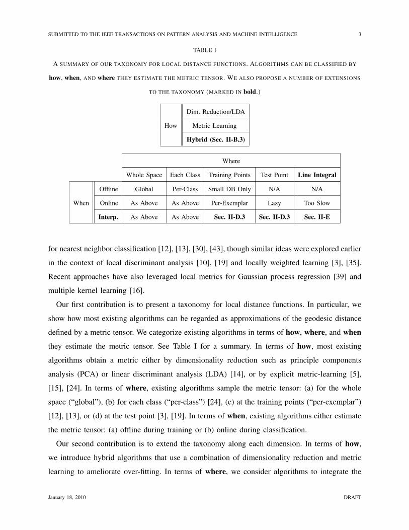
TABLE I

A SUMMARY OF OUR TAXONOMY FOR LOCAL DISTANCE FUNCTIONS. ALGORITHMS CAN BE CLASSIFIED BY

how, when, AND where THEY ESTIMATE THE METRIC TENSOR. WE ALSO PROPOSE A NUMBER OF EXTENSIONS

TO THE TAXONOMY (MARKED IN bold.)

How

Dim. Reduction/LDA

Metric Learning

Hybrid (Sec. II-B.3)

Where

Whole Space Each Class Training Points Test Point Line Integral

When

Offline Global Per-Class Small DB Only N/A N/A

Online As Above As Above Per-Exemplar Lazy Too Slow

Interp. As Above As Above Sec. II-D.3 Sec. II-D.3 Sec. II-E

for nearest neighbor classification [12], [13], [30], [43], though similar ideas were explored earlier

in the context of local discriminant analysis [10], [19] and locally weighted learning [3], [35].

Recent approaches have also leveraged local metrics for Gaussian process regression [39] and

multiple kernel learning [16].

Our first contribution is to present a taxonomy for local distance functions. In particular, we

show how most existing algorithms can be regarded as approximations of the geodesic distance

defined by a metric tensor. We categorize existing algorithms in terms of how, where, and when

they estimate the metric tensor. See Table I for a summary. In terms of how, most existing

algorithms obtain a metric either by dimensionality reduction such as principle components

analysis (PCA) or linear discriminant analysis (LDA) [14], or by explicit metric-learning [5],

[15], [24]. In terms of where, existing algorithms sample the metric tensor: (a) for the whole

space (“global”), (b) for each class (“per-class”) [24], (c) at the training points (“per-exemplar”)

[12], [13], or (d) at the test point [3], [19]. In terms of when, existing algorithms either estimate

the metric tensor: (a) offline during training or (b) online during classification.

Our second contribution is to extend the taxonomy along each dimension. In terms of how,

we introduce hybrid algorithms that use a combination of dimensionality reduction and metric

learning to ameliorate over-fitting. In terms of where, we consider algorithms to integrate the



metric tensor along the line between the test point and the training point. We present an exact

polynomial time algorithm to compute the integral under the assumption that the metric tensor

is piecewise constant. In terms of when, we consider a combined online-offline algorithm. In

the offline training phase, a representation of the metric tensor is estimated by sampling it at a

number of reference points. In the online phase, the metric tensor is estimated by interpolating

the samples at the reference points.

Our third contribution is to present a comprehensive evaluation of the algorithms in our

framework, both prior and new. We show results on a diverse set of problems, including face

recognition using MultiPIE [18], object recognition using Caltech 101 [11], and digit recognition

using MNIST [27]. To spur further progress in this area and allow other researchers to compare

their results with ours, we will make the raw feature vectors, class membership data, and training-

test partitions of the data available on a website with the goal of defining a standard benchmark1.

II. TAXONOMY AND ALGORITHMS

We now present our framework for local distance functions. We begin in Section II-A by

describing the scenario and class of functions that we consider. We introduce the metric tensor and

explain how it defines the geodesic distance. In Section II-B we describe how the core distance

functions can be learnt using either dimensionality reduction or metric learning and extend the

framework to include hybrid algorithms. In Section II-C we describe how several well-known

local distance functions can be viewed as approximations to the geodesic distance by sampling

the metric tensor at the appropriate point(s). In Section II-C we only consider algorithms that can

(at least conceptually) be applied before the test point is known. In Section II-D we consider

the time at which the metric tensor is estimated or sampled. Besides offline algorithms, we

consider online algorithms that require the test point to be known before they can be applied.

We also extend the framework to algorithms that first estimate the metric tensor at a number

of reference points and then interpolate them during online classification. In Section II-E we

present a polynomial time algorithm to integrate the metric tensor along the lines between the

test and training points.

1Available at http://www.ics.uci.edu/˜dramanan/localdist/



A. Background

1) Problem Scenario: We assume that we are working with a classification problem defined

in a K dimensional feature space RK . Each test sample is mapped into this space by computing

a number of features to give a point x ∈ RK . Similarly, each training sample is mapped into

this space to give a point xi ∈ RK . Where appropriate, we denote the test point by x and

the training points by xi. We do not consider problems where all that can be computed is the

pairwise distance or kernel matrix between each pair of test and training sample Dist(x,xi).

A number of learning algorithms have been proposed for this more general setting [12], [13].

Note, however, that such general metrics often measure the distance between two images under

some correspondence of local features and that approximate correspondence can be captured by

a pyramid vector representation [17]. An important alternate class of models define similarity

using a kernel function or weighted combination of kernel functions [4], [9], [21], [40]. Mercer’s

theorem guarantees that kernels implicitly embed data points in a feature space [9]. This feature

space is typically finite dimensional. Example kernels commonly used in image matching include

the intersection kernel and pyramid match kernel [17], [17], [29]. Notable exceptions include

the Gaussian kernel. Many, if not most, distance functions either explicitly or implicitly embed

data in a finite dimensional vector space. Our work applies to this common case.

2) Set of Distance Functions Considered: We consider distance functions that can be written

in the form:

DistM(x,xi) = (xi − x)TM(xi − x). (1)

where M is a K × K symmetric, positive definite matrix. The set of functions defined by

Equation (1) are metrics. In this paper, we interchangeably refer to the functions of the form

in Equation (1) and the matrices M as metrics, even though not all metrics can be written in

that form. Most existing algorithms, with the notable exceptions of [12], [13], consider the set

of metrics in Equation (1), or a subset of them. In many cases the positive definite condition

is relaxed to just non-negativity in which case, strictly speaking M is a psuedometric. In other

cases, only diagonal M are considered.

3) The Metric Tensor: The metric tensor is a generalization of a single constant metric of

the form in Equation (1) to a possibly different metric at each point in the space [1], [2]. The

most common use of the metric tensor is to define distances on a manifold. In our case the



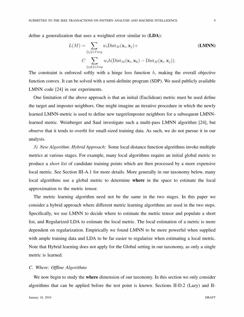
Train point

Test point

Fig. 1. An illustration of the geodesic distance defined by a metric tensor. We visualize metrics sampled at grid

points in R2 by displaying the isocontour of equivalent distances. The length of a particular path between the red

and black points is computed by integrating the metric tensor along the path. The geodesic distance is the minimum

length path, over all such paths. The shortest path is shown as the dotted curve above.

manifold is RK which has a global coordinate system. We therefore do not need to worry about

the coordinate transforms between the tensor representations, but instead can represent it as a

single matrix MT (x) at each point x in the space. Roughly speaking, MT (x) can be thought

of as defining a local distance function or metric DistMT (x) at each point in the space.

4) Geodesic Distance: Given a piecewise differentiable curve c(λ), where λ ∈ [0, 1], the

length of the curve is given by:

Length(c(λ)) =

∫ 1

0

[dc

dλ

]T

MT (c(λ))dc

dλdλ. (2)

The geodesic distance between a pair of test and training points is the distance of the shortest

curve between them:

DistGeo(x,xi) = minc(0)=x,c(1)=xi

Length(c(λ)). (3)

In Figure 1 we illustrate the metric tensor and the geodesic distance between a test point and

a training point. We visualize the metrics sampled at grid points by displaying the isocontour

of equivalent distances, which in R2 are ellipses. The shortest path between two points is not

necessarily the straight line between them, but in general is curved.

If the metric tensor is (close to) zero within each class, and has a large non-zero component

across the boundary of each class, then theoretically perfect classification can be obtained in the



absence of noise using the geodesic distance and just a single training sample in each connected

component of each class. Estimating such an ideal metric tensor would require a very dense

sampling of training data, in which case classification using nearest neighbors and a Euclidean

metric would work well. But at heart, we argue that all local distance function algorithms are

based on the hope that better classification can be obtained for typical training data densities by

using a spatially varying metric tensor and an approximation to the geodesic distance.

We now introduce our taxonomy and describe the possible choices for a local distance

function-based algorithm in terms of how, when, and where it estimates the metric tensor

and approximates the geodesic distance. We demonstrate that the interpretation of local distance

functions as approximating geodesics allows for a unification of many approaches under a general

taxonomy, as well as suggesting new algorithms.

B. How

The first component in our taxonomy is how the metric tensor is estimated at any given point

(or region) in the space in terms of a number of training samples close to that point.

1) Dimensionality Reduction Algorithms: Perhaps the simplest metric learning algorithms

are the various linear dimensionality reduction algorithms. For example, Principle Components

Analysis (PCA) [14] projects the data into a low-dimensional subspace and then measures

distance in the projected space. If P is the (orthonormal) d × K dimensional PCA projection

matrix, the corresponding distance between a pair of test and training points:

||P (xi − x)||2 = (xi − x)TMPCA(xi − x) (4)

where MPCA = PTP is the corresponding metric. Rather than an explicit projection, one can

use a Mahalanobis distance [14] (the inverse of the sample covariance matrix.)

A more powerful approach is to learn a subspace that preserves the variance between class

labels using Linear Discriminant Analysis (LDA) [14]. LDA has a large number of variants.

In this paper we consider a weighted form of Regularized LDA [14] described below. We

assume we are given a set of triples {xi, yi, wi} consisting of data points, class labels, and

weights. We can interpret integer weights as specifying the number of times an example appears

in an equivalent unweighted dataset. We search for the d × K dimensional LDA basis V that



maximizes:

arg maxV

tr(V T ΣBV ) s.t. V T (ΣW + λI)V = I (LDA)

ΣB =1

C

∑j

µ̄jµ̄Tj , ΣW =

∑iwix̄ix̄

Ti∑

iwi

, x̄i = xi − µyi

µ̄j = µj −1

C

∑j

µj, µj =

∑{i:yi=j}wixi∑{i:yi=j}wi

where C is the number of classes. This can be solved with a generalized eigenvalue problem.

Because the rank of ΣB is upper bounded by C and generally C < K we use a bagged estimate

of ΣB obtained by averaging together covariance matrices estimated from sub-sampled data

[42]. The regularization parameter λ enforces an isotropic Gaussian prior on ΣW that ensures

that the eigenvalue problem is well conditioned when ΣW is low rank. We found this explicit

regularization was essential for good performance even when ΣW is full rank. We used a fixed

λ = 1 for all our experiments.

As defined in Equation (LDA), V is not guaranteed to be orthonormal. We explicitly apply

Gram-Schmidt orthonormalization to compute VG and define the LDA metric: MLDA = V TG VG

where MLDA is a K × K matrix of rank d. An alternative approach [19] is to use the scatter

matrices directly to define a full-rank metric M = S−1W SBS

−1W . Empirically, we found the low-

rank metric MLDA to perform slightly better, presumably due to increased regularization.

2) Metric Learning Algorithms: Recently, many approaches have investigated the problem

of learning a metric M that minimizes an approximate K-NN error on a training set of data

and class label pairs {xi, yi} [5], [15], [23], [24], [38]. Relevant Component Analysis (RCA)

[5] finds the basis V that maximizes the mutual information between xi and its projection V xi

while requiring that that distances between projected points from the same class remain small.

Neighborhood Component Analysis (NCA) [15] minimizes a probabilistic approximation of the

leave-one-out cross validation error. Recent approaches minimize a hinge-loss approximation of

the misclassification error [23], [24], [38].

The state-of-the-art at the time of writing appears to be the Large Margin Nearest Neighbor

(LMNN) algorithm [24]. LMNN defines a loss function L that penalizes large distances between

“target” points that are from the same class while enforcing the constraint that, for each point i,

“imposter” points k from different classes are 1 unit further away than target neighbors j. We



define a generalization that uses a weighted error similar to (LDA):

L(M) =∑

{ij}∈Targ

wiDistM(xi,xj)+ (LMNN)

C∑

{ijk}∈Imp

wih(DistM(xi,xk)−DistM(xi,xj)).

The constraint is enforced softly with a hinge loss function h, making the overall objective

function convex. It can be solved with a semi-definite program (SDP). We used publicly available

LMNN code [24] in our experiments.

One limitation of the above approach is that an initial (Euclidean) metric must be used define

the target and imposter neighbors. One might imagine an iterative procedure in which the newly

learned LMNN-metric is used to define new target/imposter neighbors for a subsequent LMNN-

learned metric. Weinberger and Saul investigate such a multi-pass LMNN algorithm [24], but

observe that it tends to overfit for small-sized training data. As such, we do not pursue it in our

analysis.

3) New Algorithm: Hybrid Approach: Some local distance function algorithms invoke multiple

metrics at various stages. For example, many local algorithms require an initial global metric to

produce a short list of candidate training points which are then processed by a more expensive

local metric. See Section III-A.1 for more details. More generally in our taxonomy below, many

local algorithms use a global metric to determine where in the space to estimate the local

approximation to the metric tensor.

The metric learning algorithm need not be the same in the two stages. In this paper we

consider a hybrid approach where different metric learning algorithms are used in the two steps.

Specifically, we use LMNN to decide where to estimate the metric tensor and populate a short

list, and Regularized LDA to estimate the local metric. The local estimation of a metric is more

dependent on regularization. Empirically we found LMNN to be more powerful when supplied

with ample training data and LDA to be far easier to regularize when estimating a local metric.

Note that Hybrid learning does not apply for the Global setting in our taxonomy, as only a single

metric is learned.

C. Where: Offline Algorithms

We now begin to study the where dimension of our taxonomy. In this section we only consider

algorithms that can be applied before the test point is known. Sections II-D.2 (Lazy) and II-



Test point

Per−class metricsmetrics

Per−exemplar

Class2

Class3

metricGlobal

Class1

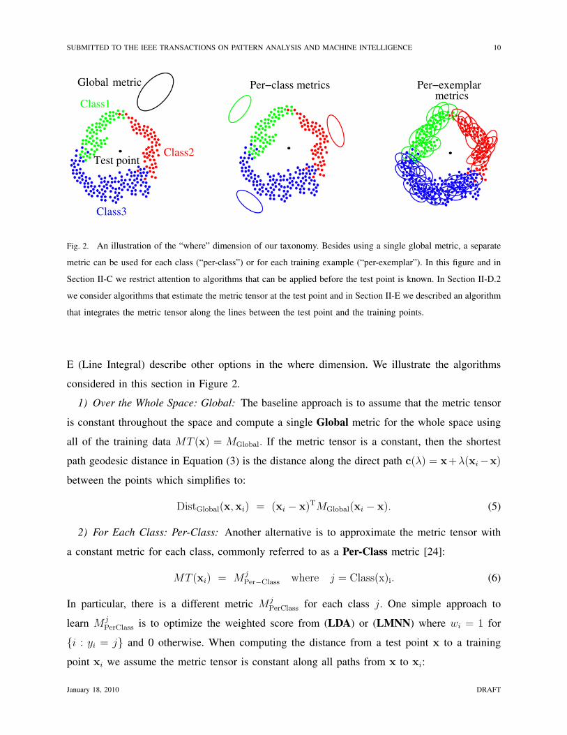
Fig. 2. An illustration of the “where” dimension of our taxonomy. Besides using a single global metric, a separate

metric can be used for each class (“per-class”) or for each training example (“per-exemplar”). In this figure and in

Section II-C we restrict attention to algorithms that can be applied before the test point is known. In Section II-D.2

we consider algorithms that estimate the metric tensor at the test point and in Section II-E we described an algorithm

that integrates the metric tensor along the lines between the test point and the training points.

E (Line Integral) describe other options in the where dimension. We illustrate the algorithms

considered in this section in Figure 2.

1) Over the Whole Space: Global: The baseline approach is to assume that the metric tensor

is constant throughout the space and compute a single Global metric for the whole space using

all of the training data MT (x) = MGlobal. If the metric tensor is a constant, then the shortest

path geodesic distance in Equation (3) is the distance along the direct path c(λ) = x+λ(xi−x)

between the points which simplifies to:

DistGlobal(x,xi) = (xi − x)TMGlobal(xi − x). (5)

2) For Each Class: Per-Class: Another alternative is to approximate the metric tensor with

a constant metric for each class, commonly referred to as a Per-Class metric [24]:

MT (xi) = M jPer−Class where j = Class(x)i. (6)

In particular, there is a different metric M jPerClass for each class j. One simple approach to

learn M jPerClass is to optimize the weighted score from (LDA) or (LMNN) where wi = 1 for

{i : yi = j} and 0 otherwise. When computing the distance from a test point x to a training

point xi we assume the metric tensor is constant along all paths from x to xi:



DistPC(x,xi) = (xi − x)TMClass(xi)Per−Class(xi − x). (7)

Generally speaking, metrics learned for each class may not be comparable, since they are

trained independently. Similar issues arise in multiclass learning because multiple one-versus-all

classifiers may not be directly comparable, although in practice, such a strategy is often employed

[33]. We make LDA metrics comparable by normalizing each to have a unit trace. We fix the

rank d of the LDA metric to be the number of distinct classes present amount the neighbors

of the training examples of class j. To normalize the LMNN metrics, we follow the approach

introduced in [13] and [24] and define a generalization of Equation (LMNN) that learns metrics

Mc for all the classes together:

L({Mc}) =∑

{ij}∈Targ

DistMyi(xi,xj)+ (8)

C∑

{ijk}∈Imp

h(DistMyi(xi,xk)−DistMyi

(xi,xj)).

3) At the Training Points: Per-Exemplar: Another approximation is to assume that the metric

tensor is constant within the neighborhood of each training sample xi and use a Per-Exemplar

metric:

MT (x) = MxiPer−Exemplar (9)

for points x close to xi. An example of the Per-Exemplar approach, used in a more general non-

metric distance function, is [12], [13]. A simple approach to learn MxiPer−Exemplar is to optimize

Equation (LDA) or (LMNN) with neighboring points weighted by one (wi = 1) and far away

points are weighted by (wi = 0). As in LMNN, an initial metric must be used to construct these

neighbors. We found that a global metric, learned with either LDA or LMNN (as dictated by

the “How” taxonomy criterion), outperformed a Euclidean metric for the purposes of identifying

neighbors.

Again, these local metrics may not be comparable. As before, we trace-normalize the LDA

metrics. In theory, one can define an extension of Equation (8) that simultaneously learns all

LMNN exemplar metrics. This is infeasible due to the number on training exemplars, and so we

independently learn LMNN exemplar metrics. In practice, this still performs well because the

initial pruning step (creating a shortlist) tends to select close-by exemplars whose metrics are

learned with similar data.



When computing the distance from a test point x to a training point xi we assume the metric

tensor is constant along all paths from x to xi and so use the metric of xi:

DistPE(x,xi) = (xi − x)TMxiPer−Exemplar(xi − x). (10)

D. When

We now consider the when dimension of our taxonomy. We first consider traditional algo-

rithms, both offline and online. Afterwards we present an interpolation algorithm which estimates

the metric tensor at a number of reference points in an offline phase and then interpolates these

estimates in the online classification phase.

1) Offline: Offline algorithms compute the metric at train time, before any test points are given.

In Table I only the Global, Per-Class and Per-Exemplar algorithms could be used offline. The

Lazy and Line Integral approaches require the test point and so cannot be applied. The Global

approach is the most common [5], [15], [23], [24], [38], and also the least computationally

demanding. Given a dataset with M training points in C classes in a K dimensional space, just

a single metric must be estimated and the storage requirement is only O(K2). The Per-Class

approach [24] must estimate C metrics, and so requires storing O(CK2). A non-metric variant

of the Per-Exemplar approach has also been used in the past [12], [13]. Since the number of

training points M is typically much larger than the number of classes, the storage cost O(MK2)

can make the application of this approach in an offline fashion intractable for very large datasets

including ours. One can, however, define an “online” Per-Exemplar that first computes a short-

list of exemplars for a test point using a global metric. One can then learn metrics of each

short-listed exemplar on-the-fly, use them to re-rank the exemplars, and discard them without

any need for storage. We include this algorithm in our experiments.

2) Online at the Test Point: Lazy: Once the test point has been provided during the online

classification phase, another option is to estimate the metric tensor at the test point:

MT (x) = MxLazy. (11)

See Figure 3(left) for an illustration. This approach requires learning the metric at run time

which is why we refer to it as Lazy. The training set for the Lazy algorithm consists of S

training points xi close to the test point x. In our experiments, we use a Global metric to define

which points are the closest and set S = 50. We set wi for these training points to be 1 and



Lazy Smooth interpolation

Test points Reference points

NN−interpolationTest point

Fig. 3. An illustration of the “when” dimension of our taxonomy. Left: The Lazy algorithm estimates the metric

tensor at the test point, which shifts the computation online. An obvious drawback of the Lazy approach is

the computational cost. Middle: Our interpolation algorithm precomputes the metric tensor at a small subset of

reference points. The online metric is computed by interpolating the metrics at the reference points. We describe

two approaches using radial basis functions (Middle) and simple NN-interpolation. With proper construction of the

reference metrics, NN-interpolation can perform similarly to Lazy with a reduction in computational cost. Right:

NN-interpolation carves up the vector space into an anisotropic Voronoi diagram with quadratic boundaries between

Voronoi cells [25].

0 otherwise, and optimize Equation (LDA) or (LMNN) to learn MxLazy. We fix the rank d of

the LDA metric to the number of distinct classes present in the S training neighbors. When

computing the distance from a test point x to a training point xi we assume the metric tensor

is constant along all paths from x to xi and use the metric estimated at the test point x:

DistLazy(x,xi) = (xi − x)TMxLazy(xi − x). (12)

Examples of the Lazy algorithm are the local discriminant adaptive algorithm of [19], the locally

weighted learning algorithm of [3], and the locally adaptive metric algorithm of [10]. These

algorithms all use a global metric to select the S nearest neighbors of a test point x which are

then classified using a locally learnt distance function. Zhang et al [43] use a similar approach,

but directly learn a local discriminant boundary using an SVM rather than learning a local metric.

3) New Algorithms: Interpolation: We expect the metric tensor MT (x) to vary smoothly. This

suggests that we can interpolate the metric tensor from a sparse set of samples. Assume that a

subset of the training examples has been selected. We refer to these points xRPi for i = 1, . . . , R

as reference points. We use radial basis function interpolation to interpolate the metric tensor

in the remaining parts of the space [7]. In our experiments we chose the reference points at



random, however, a more principled approach to distribute the reference points uniformly could

have been used.

Offline, local metrics MxRPiRP are computed for the reference points by optimizing Equa-

tion (LDA) or (LMNN) with wRPi = 1 and 0 otherwise. One could learn these metrics jointly

but we found independently learning the metrics sufficed. Online, the local metrics MxRPiRP are

interpolated to obtain the final metric. One approach is nearest neighbor (NN) interpolation:

MTNN(x) = MxRPiRP where i = argmin

jDistGlobal(x,xRPj). (13)

Here we use a Global metric to define closeness to the references points. Another approach

would be to use that reference point’s own metric, as is done in Section II-E. We saw similar

performance in either case with a slight speed up with Global. Another approach would be to

use a smooth weighted average of the metrics obtained through radial basis function (RBF)

interpolation [7]:

MTRBF (x) =R∑

i=1

wi(x)MxRPiRP (14)

wi(x) =e−

1σ

DistGlobal(x,xRPi)∑R

j=1 e− 1σ

DistGlobal(x,xRPj). (15)

In our experiments, we varied σ between .01 and .001, set by cross validation. We used a fixed

number of R = 500 reference points and observed consistent behavior at both double and half

that amount . Given a fixed DistGlobal, we can compute wij = wj(xi). Interpreting these values

as the probability that training point xi selects metric MxRPj

RP , we can learn each MxRPj

RP so as

to minimize expected loss by optimizing Equation (LDA) and (LMNN) with weights wij . One

could define a weighted version of Equation (8) that simultaneously learns all reference metrics.

Since this involves a sum over the cross product of all imposter triples with all reference points,

we chose not to do this.

We found empirically at first that the smooth weighted average metric in Equation (14) signif-

icantly outperformed the nearest neighbor algorithm. The computational cost of computing the

smooth weighted average metric in Equation (14) is significantly more, however. Subsequently

we found a different way of training the metrics at the reference points that largely eliminates

this difference in performance. We now describe this approach.



We hypothesized that the smooth interpolation outperformed NN interpolation because the

smoothing acted as an additional regularizer. To achieve the same regularization effect for NN

interpolation, we applied a cross-validation step to construct a regularized version of MxRPiRP :

MxRPj

CV =1

Zj

∑i 6=j

wi(x)MxRPiRP (16)

where Zj is a normalization factor included to ensure the sum of weights wi(x) for j 6= i is

1, and wi(x) is defined as in Equation (15). MxRPiCV is equivalent to the metric tensor computed

at x = xRPi using Equation (14) but limiting the summation to include only the R − 1

other reference points. We found MTNN(x) computed with the above cross-validated metrics

performed similarly to MTRBF (x), but was significantly faster. As such, our interpolation results

reported in our experiments are generated with NN interpolation with MxRPj

CV .

So far we have described the interpolation of the reference point metrics for the test point x.

The same interpolation could be performed anywhere in the feature space. For example, it could

be performed at the training points xi. This leads to a space-efficient version of Per-Exemplar.

Another use of the interpolation algorithm is to compute the Line Integral of the metric tensor

between the train and test points. We now describe this algorithm.

E. New Algorithms: Integration Along the Line Between Train and Test Points

Computing the geodesic distance in Equation (3) in high dimensions is intractable. In 2D or

3D the space can be discretized into a regular grid of vertices (pixels/voxels) and then either

an (approximate) distance transform or a shortest path algorithm used to estimate the geodesic

distance. In higher dimensions, however, discretizing the space yields a combinatorial explosion

in the number of vertices to be considered. To avoid this problem, all of the above algorithms

assume that the metric tensor is locally (or globally) constant and so can approximate the geodesic

distance with the simple metric distance in Equation (1).

One way to obtain a better approximation of the geodesic is to assume that the space it not

curved locally and approximate the minimum in Equation (3) with the integral along the line

between the test point x and the training point xi:

c(λ) = x + λ(xi − x). (17)



Substituting Equation (17) into Equation (2) and simplifying yields the Line Integral distance:

DistLine(x,xi) = (xi − x)T

[∫ 1

0

MT (c(λ)) dλ

](xi − x). (18)

Note that the line distance is an upper bound on the geodesic distance:

DistGeo(x,xi) ≤ DistLine(x,xi). (19)

We now present a polynomial time algorithm to estimate the integral in Equation (18) exactly

under the assumption that the metric tensor is piecewise constant, and using the nearest-neighbor

interpolation algorithm in Section II-D.3.

We assume that the metric tensor has been sampled at the reference points to estimate MxRPiRP .

We also assume that the metric tensor is piecewise constant and its value at any given point x

is the value at the reference point which is closest, as measured by that reference points metric:

MT (x) = MxRPiRP (20)

where for all j = 1, . . . , R:

(x− xRPi)TM

xRPiRP (x− xRPi) ≤ (x− xRPj)

TMxRPj

RP (x− xRPj). (21)

Equation (21) divides the space into an “anisotropic Voronoi diagram” similarly to [25]. See

Figure 3(right) for an illustration. The Voronoi diagram is anisotropic because the metric is

different in each cell, whereas for a regular Voronoi diagram there is a single global metric.

Equation (21) defines R(R − 1)/2 boundary surfaces, one between each pair of references

points. There could, however, be an exponential number of cells as the addition of each new

boundary surface could divide all of the others into two or more sub-cells.

To compute the integral in Equation (18) we need to break the domain λ ∈ [0, 1] into the

segments for which it is constant. The boundaries of the regions in Equation (21) are defined

by the equalities:

(x− xRPi)TM

xRPiRP (x− xRPi) = (x− xRPj)

TMxRPj

RP (x− xRPj). (22)

Equation (22) is a quadratic and in general the solution is a quadratic hyper-surface. The

intersection of this boundary hypersurface and the line between the test and training points

in Equation (18) can be computed by substituting Equation (18) into Equation (22). The result



xtest

xtrain

xRP1

xRP2

xRP3

B12

B23

B13

l123

l223

l112

l113

l=0

l=1

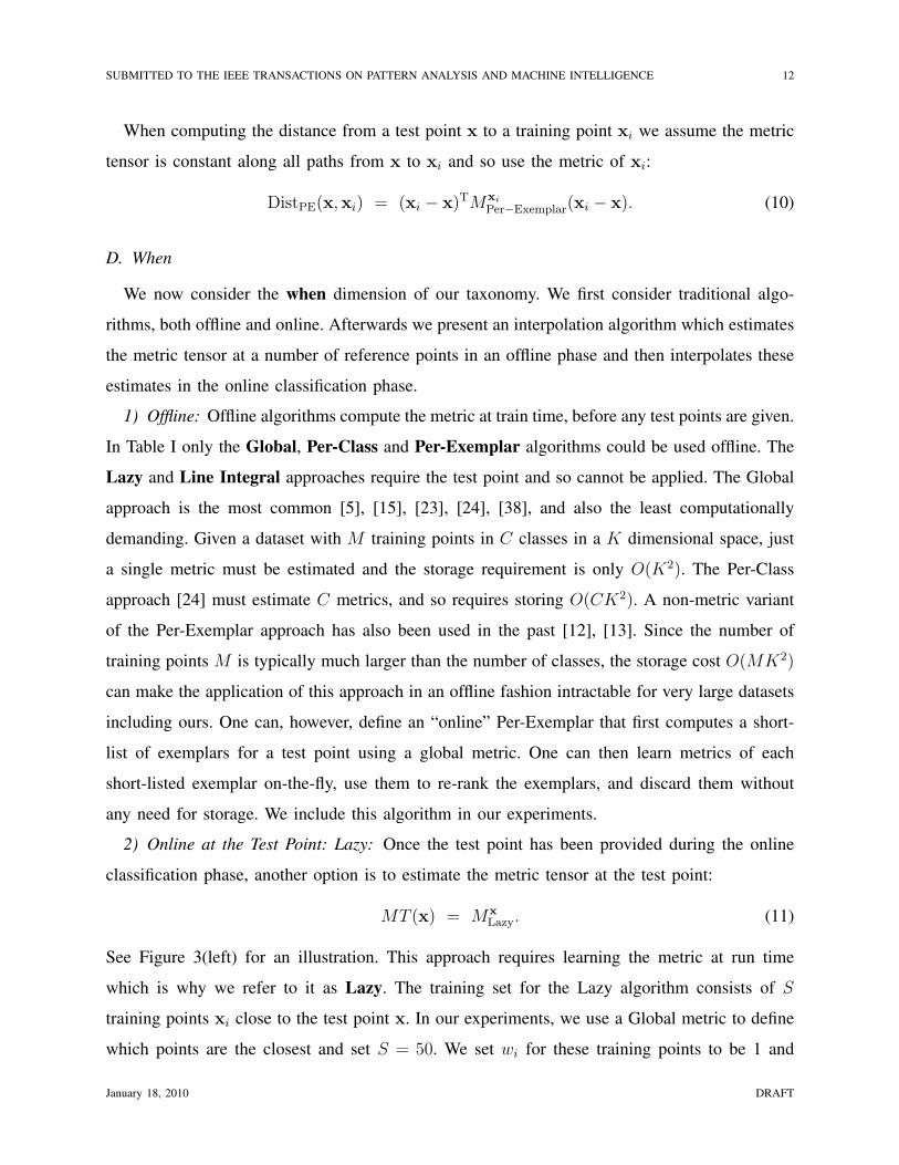
Fig. 4. An illustration of the computation of the exact polynomial integration of the metric tensor along the line

from the training point to the test point under the assumption that the metric tensor is piecewise constant. In this

example there are three reference points xRP1 , xRP2 , and xRP3 . The regions in space where the metric tensor is

constant are bounded by quadratic hypersurfaces, in this case denoted B12, B23, and B13. The intersection of these

hypersurfaces and the line between the test point xtest and the training point xtrain can be computed by solving

a quadratic in the single unknown λ. The solutions for λ that lie in the interval [0, 1] can be sorted and then the

integral approximated by adding up the length of the results segments, after searching for the appropriate reference

point to use for each segment.

is a quadratic in the single unknown λ which can be solved to give either 0, 1 or 2 solutions in

the range [0, 1].

Once all the solutions that lie in λ ∈ [0, 1] have been computed, they can be sorted. This breaks

the line in Equation (18) into a number of segments where the metric tensor is constant on each

one. The appropriate value of the metric tensor is then computed for each such segment by taking

the midpoint of the segment and computing the closest reference point using Equation (21). The

lengths of all the segments can then be computed and added up. In total, there can be at most

2R(R − 1)/2 intersection points. Computing each one takes time O(K2). There are at most

1 + R(R − 1) segments of the line between the test and training points. The search for the

closest reference point for each one takes O(RK2) because there are R reference points and the

cost of computing the distance to it is O(K2). The total computation cost is therefore polynomial



O(R3K2).

III. EXPERIMENTS

We now present our experimental results. We describe the databases and how we sample them

in Section III-A. We also describe two implementation details. In Section III-A.1 we describe

candidate pruning. In Section III-A.2 we describe indexing structures. We describe the evaluation

metrics and the result in Section III-B. We include some of the results in the Appendix, in tabular

form following the taxonomy outlined in Figure I. The complete set of results are included in

the online supplemental material at the author’s website. In Section III-C we analyze the results

in detail, plotting various interesting subsets.

A. Databases and Data Sampling

We compared the various algorithms on a diverse set of problems, including face recognition

using MultiPIE [18], object recognition using Caltech 101 [11], and digit recognition using

MNIST [27]. In Figure 5 we include a number of example images from each of the 3 databases.

MultiPIE [18] is a larger version of the CMU PIE database [36] that includes over 700,000

images of over 330 subjects collected in four sessions over six months. We extract the face

regions automatically in the five frontal-most cameras (-45 degrees to +45 degrees) using the

Viola-Jones face detector [41]. The face regions were then resampled and normalized to 80×80

grayscale patches with zero mean and unit variance. The patches were then projected into their

first 254 principle components (95% of the empirical variance.) Different sessions were used as

training and testing data. We randomly generated 10 batches of 1000 examples as our test sets.

Caltech 101 [11] is a widely used benchmark for image classification consisting of over 9,000

images from 101 object categories. We base our results on the widely-used single-cue baseline

of spatial pyramid kernels [26]. We use the publicly available feature computation code from

the author’s website, which generates a sparse feature vector of visual word histograms for each

image. We project the vectors such that 95% of the variance is captured, and then use them

in our local distance function framework. We follow the established protocol of leave-one-out

cross validation with 30 training examples per class. Using the online implementation provided

by the author, we obtained an average classification rate of 62.18, slightly below the reported



Fig. 5. Example images extracted from the 3 databases that we used. Bottom Left: MultiPIE [18]. Right: Caltech 101 [11].

Top Left: MNIST [27].

value of 64.6. Recent work exploiting multiple cues has improved this score [6], [21], [40], but

we restrict ourselves to this established baseline for our analysis.

MNIST [27] is a well-studied dataset of 70,000 examples of digit images. We followed the

pre-processing steps outlined by [24]. The original 28× 28 dimensional images were deskewed

and projected into their leading 164 principle components which were enough to capture 95% of

the data variance. The normal MNIST train/test split [27] has two problems. (1) The training data

is very dense with error rates around 1-2% making it hard to see any difference in performance.

(2) There is only one partition making it impossible to estimate confidence intervals. To rectify

these problems, we sub-sampled both the train and test data, in 10 batches of 1000 examples.

1) Candidate Pruning: Many of the algorithms in our taxonomy, though polynomial in space

and time, can still be computationally demanding. In all cases we apply a short-listing approach

similar to that used in previous work [3], [19], [43]. We first prune the large set of all candidate

matches (the training points) with a global metric. In Figure 6 we consider the effect of varying

the pruning threshold for three algorithms on the MultiPIE experiments. We find the recognition



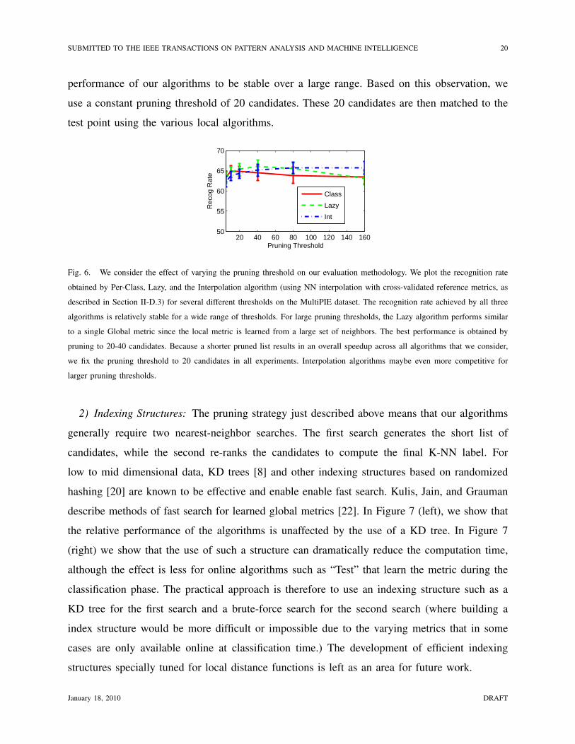
performance of our algorithms to be stable over a large range. Based on this observation, we

use a constant pruning threshold of 20 candidates. These 20 candidates are then matched to the

test point using the various local algorithms.

20 40 60 80 100 120 140 16050

55

60

65

70

Pruning Threshold

Rec

og R

ate

Class

Lazy

Int

Fig. 6. We consider the effect of varying the pruning threshold on our evaluation methodology. We plot the recognition rate

obtained by Per-Class, Lazy, and the Interpolation algorithm (using NN interpolation with cross-validated reference metrics, as

described in Section II-D.3) for several different thresholds on the MultiPIE dataset. The recognition rate achieved by all three

algorithms is relatively stable for a wide range of thresholds. For large pruning thresholds, the Lazy algorithm performs similar

to a single Global metric since the local metric is learned from a large set of neighbors. The best performance is obtained by

pruning to 20-40 candidates. Because a shorter pruned list results in an overall speedup across all algorithms that we consider,

we fix the pruning threshold to 20 candidates in all experiments. Interpolation algorithms maybe even more competitive for

larger pruning thresholds.

2) Indexing Structures: The pruning strategy just described above means that our algorithms

generally require two nearest-neighbor searches. The first search generates the short list of

candidates, while the second re-ranks the candidates to compute the final K-NN label. For

low to mid dimensional data, KD trees [8] and other indexing structures based on randomized

hashing [20] are known to be effective and enable enable fast search. Kulis, Jain, and Grauman

describe methods of fast search for learned global metrics [22]. In Figure 7 (left), we show that

the relative performance of the algorithms is unaffected by the use of a KD tree. In Figure 7

(right) we show that the use of such a structure can dramatically reduce the computation time,

although the effect is less for online algorithms such as “Test” that learn the metric during the

classification phase. The practical approach is therefore to use an indexing structure such as a

KD tree for the first search and a brute-force search for the second search (where building a

index structure would be more difficult or impossible due to the varying metrics that in some

cases are only available online at classification time.) The development of efficient indexing

structures specially tuned for local distance functions is left as an area for future work.



Global Class Lazy0

10

20

30

40MultiPIE Timing(sec)

Brute−force

KDTree

Global Class Lazy50

55

60

65

70MultiPIE Recognition Rate

Rec

og

Rat

e

Tim

ing

(sec

)

Where Where

Fig. 7. We consider the effect of efficient indexing structures on our evaluation methodology. Using the MultiPIE dataset, we

compare algorithms that vary along the “Where” dimension using a brute-force NN search versus a KD-tree based search. The

KD-tree is only used during the initial candidate pruning stage. As shown above, algorithms whose computationally requirements

are focused on the initial stage – such as Global or Per-Class – can see a significant speed up at the cost of a small decrease in

performance. However, some of the algorithms we consider spend more computational effort on the second stage of re-ranking,

making the efficiency of the initial indexing less prominent in the total computation time. An example is the Lazy algorithm that

learns a metric at test-time. For simplicity, we present all timing results using a brute-force linear scan across all our experiments.

B. Evaluation Measures and Results

We obtain a final classification for each algorithm by applying K-NN with K = 3 on the

re-ranked shortlisted neighbors of a test point. We computed a variety of evaluation measures.

In particular, we computed (1) recognition rates, (2) error rates, (3) percentage reduction in the

error rate from the global baseline, and (4) computation times. For each measure, we computed

both the average values and the standard deviations across the sets of test samples (10 for Multi-

PIE and MNIST, and 30 for Caltech 101.) In the appendix we include a set of tables containing

all of the recognition rate and computation time results. We include the full set of results for

all four measures of performance in a set of interactive webpages in the online supplemental

material.

C. Analysis of the Results

We now discuss the results in the context of our taxonomy of local distance functions. The

criteria we consider for evaluation are both accuracy and computational cost. We perform a

greedy exploration of our taxonomy, iteratively exploring dimensions given the best performing

algorithm encountered thus far.



PCA LDA Metric50

55

60

65

70

MultiPIE

PCA LDA Metric30

35

40

45

50

55

60

Caltech

PCA LDA Metric90

92

94

96

98

100

MNIST

Rec

og

Rat

e

Algorithm Algorithm Algorithm

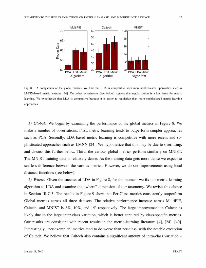
Fig. 8. A comparison of the global metrics. We find that LDA is competitive with more sophisticated approaches such as

LMNN-based metric learning [24]. Our other experiments (see below) suggest that regularization is a key issue for metric

learning. We hypothesize that LDA is competitive because it is easier to regularize than more sophisticated metric-learning

approaches.

1) Global: We begin by examining the performance of the global metrics in Figure 8. We

make a number of observations. First, metric learning tends to outperform simpler approaches

such as PCA. Secondly, LDA-based metric learning is competitive with more recent and so-

phisticated approaches such as LMNN [24]. We hypothesize that this may be due to overfitting,

and discuss this further below. Third, the various global metrics perform similarly on MNIST.

The MNIST training data is relatively dense. As the training data gets more dense we expect to

see less difference between the various metrics. However, we do see improvements using local

distance functions (see below).

2) Where: Given the success of LDA in Figure 8, for the moment we fix our metric-learning

algorithm to LDA and examine the “where” dimension of our taxonomy. We revisit this choice

in Section III-C.3. The results in Figure 9 show that Per-Class metrics consistently outperform

Global metrics across all three datasets. The relative performance increase across MultiPIE,

Caltech, and MNIST is 8%, 10%, and 1% respectively. The large improvement in Caltech is

likely due to the large inter-class variation, which is better captured by class-specific metrics.

Our results are consistent with recent results in the metric-learning literature [4], [24], [40].

Interestingly, “per-exemplar” metrics tend to do worse than per-class, with the notable exception

of Caltech. We believe that Caltech also contains a significant amount of intra-class variation –



Global Class Train Test50

55

60

65

70

MultiPIE


45

50

55

60

65

70

Caltech


92

94

96

98

100

MNIST

Rec

og R

ate

Where Where Where

Fig. 9. Results across the “where” dimension of our taxonomy using LDA-based metric learning. We see that per-exemplar

(Train) does not always outperform per-class even though it is a strictly more flexible model. We hypothesize two reasons. First,

per-exemplar requires many more metrics and so tends to overfit the large number of parameters to be estimated. Second, it is

difficult to ensure the multiple metrics are normalized appropriately so that distances computed using them are fairly comparable.

The latter point is not an issue when a single metric is used centered at the test point, equivalent to classic “Lazy” approaches

to learning [3], [19]. For LDA-based metric learning, the Lazy approach performed the best for all three datasets.

at least relative to our other datasets – and that this variation is better modeled by exemplar-

specific metrics. However in general, we find that it is difficult to learn accurate per-exemplar

metrics for the two following reasons. First, per-exemplar metric learning estimates many more

metrics and so suffers from over-fitting due to the large number of parameters to be learned.

Secondly, it is difficult to ensure that multiple metrics are appropriately normalized so that the

distances computed using them are comparable. The second of these shortcomings are dealt with

by directly learning a metric at the Test point. Our experimental results in Figure 8 suggest that

such classic Lazy algorithms [3], [19] are competitive with, or even outperform, more recent

“per-class” and “per-exemplar” approaches for local metric learning. We show an example of

the Lazy algorithm in Figure 10.

3) How: Given the success of the Lazy algorithm in Figure 12, we focus on the Lazy algorithm

and re-examine the choice of the metric-learning algorithm. In Figure 11 we include results for the

“How” dimension of our taxonomy. We find that LMNN noticeably under-performs LDA-based

metric learning in the Lazy setting. We hypothesize this is the case because the second-stage

metric is learned from a small set of shortlisted neighbors. Discriminative learning approaches

such as LMNN are known to be more susceptible to overfitting [31]. LDA performs better with



1−NN

Lazy

50−NN

NN

Test

Fig. 10. Why does Lazy local metric-learning work well? We consider an example from the MultiPIE database. We show a

test image and its 50-NN, ordered by distance, under a global LDA metric. The 50-NN tend to have the same expression and

pose as the test point. However, the 1-NN happens to be incorrectly labeled. A local metric computed from these 50-NN will

be tailored to this specific expression and pose. This is in contrast to both a global and class-specific metric which must attempt

to be invariant to these factors. This makes the Lazy local metric better suited for disambiguating classes near this test point.

We show the correctly classified NN using the Lazy metric in the bottom left.

less training data because of its underlying generative modeling assumptions and because it is

straightforward to regularize. Our novel hybrid algorithm exploits the strengths of each approach,

using LMNN for the initial global search where more training data is available, and LDA for

local metric-learning where training data is sparse.

4) When: Our experimental analysis to this point suggests that the Hybrid Lazy algorithm

performs the best. One drawback of Lazy learning is its run-time cost. For certain applications,

this may be impractical. We examine tradeoffs between recognition rate and run-time in Fig-

ure 12. Comparing the best off-line approach (Per-class) with the best on-line approach (Lazy),

we see that Lazy tends to perform better but can be orders of magnitude slower. This is especially

true of LMNN-based metric-learning, which requires solving a semi-definite program (SDP) for

each test point. Our novel interpolation algorithm shifts the metric learning computation offline,

only requiring online interpolation. Interpolated metrics, while not performing as well as Lazy



LDA Metric Hybrid50

55

60

65

70Caltech

LDA Metric Hybrid90

92

94

96

98

100MNIST

LDA Metric Hybrid60

65

70

75

80MultiPIE

Reco

g R

ate

How How How

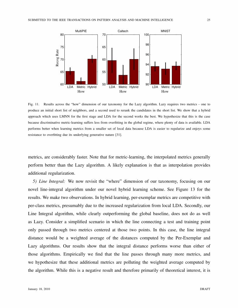
Fig. 11. Results across the “how” dimension of our taxonomy for the Lazy algorithm. Lazy requires two metrics - one to

produce an initial short list of neighbors, and a second used to rerank the candidates in the short list. We show that a hybrid

approach which uses LMNN for the first stage and LDA for the second works the best. We hypothesize that this is the case

because discriminative metric-learning suffers less from overfitting in the global regime, where plenty of data is available. LDA

performs better when learning metrics from a smaller set of local data because LDA is easier to regularize and enjoys some

resistance to overfitting due its underlying generative nature [31].

metrics, are considerably faster. Note that for metric-learning, the interpolated metrics generally

perform better than the Lazy algorithm. A likely explanation is that as interpolation provides

additional regularization.

5) Line Integral: We now revisit the “where” dimension of our taxonomy, focusing on our

novel line-integral algorithm under our novel hybrid learning scheme. See Figure 13 for the

results. We make two observations. In hybrid learning, per-exemplar metrics are competitive with

per-class metrics, presumably due to the increased regularization from local LDA. Secondly, our

Line Integral algorithm, while clearly outperforming the global baseline, does not do as well

as Lazy. Consider a simplified scenario in which the line connecting a test and training point

only passed through two metrics centered at those two points. In this case, the line integral

distance would be a weighted average of the distances computed by the Per-Exemplar and

Lazy algorithms. Our results show that the integral distance performs worse than either of

those algorithms. Empirically we find that the line passes through many more metrics, and

we hypothesize that these additional metrics are polluting the weighted average computed by

the algorithm. While this is a negative result and therefore primarily of theoretical interest, it is



OfflineOnline Interp0

50

100

150

200

250

Caltech


100

200

300

400

500

600

MNIST

OfflineOnlineInterp

200

400

600

800

1000

1200

MultiPIE

Offline Online Interp50

55

60

65

70

75

80MultiPIE


45

50

55

60

65

70Caltech


92

94

96

98

100MNIST

Run time (seconds)Recognition Rate

When

Rec

og

Rat

e

When When

Tim

ing

(se

c)

When When When

Metric Learning (LMNN) Alg


20

30

40

50

60

70MultiPIE


5

10

15

20

25

30MNIST


5

10

15

20Caltech


45

50

55

60

65

70Caltech


55

60

65

70

75

80MultiPIE


92

94

96

98

100MNIST

Run time (seconds)Recognition Rate

Rec

og

Rat

e

Tim

ing

(se

c)

When When When When When When

Hybrid Learning Alg

Fig. 12. Results for the “when” dimension of our taxonomy for both metric-learning (top) and our hybrid algorithm (bottom).

On the left we show recognition rates, while on the right we show run-times for classification. In the above graphs “off-line”

refers to Per-class metric learning, which we generally find to be a good choice for off-line metric learning. We write “on-line”

to refer to the Lazy algorithm that estimates the metric at the test point. We show results for our novel “interpolation” algorithm

that approximates Lazy while still shifting computation off-line. In LMNN metric-learning, interpolation tends to outperform

the on-line Lazy algorithm, probably due to increased regularization. In Hybrid learning, where overfitting is less of an issue,

interpolated metrics perform similarly to, or slightly worse than, their Lazy counterparts. Iterpolated metrics are significantly

faster in either case, and dramatically so for Metric Learning. We attribute the success of the off-line algorithm in MNIST to

its lack of intra-class variation (eliminating the need for a more flexible “on-line” Lazy metric estimation).

still important to show that little can be gained by such an approach.

6) Previous Reported Results: Our MultiPIE results are comparable to those reported in [18],

but are obtained automatically without manually marked fiducial locations. Our score of 60.1 on

Caltech is comparable to the score of 62.2 we obtained by running the author’s code from [26],

which itself is slightly below the reported value of 64.6. We hypothesize the chi-squared kernel

from [26] performs a form of local weighting. Our MNIST results are not directly comparable

to previous work because we use subsampled data, but our class-specific learned-metric baseline



GlobalClass Train Test Line50

55

60

65

70

75

80

MultiPIE


45

50

55

60

65

70

Caltech


92

94

96

98

100

MNIST

Where

Rec

og

Rat

e

Where Where

Fig. 13. We revisit the “where” dimension of our taxonomy using our hybrid algorithm, including results for our novel Line

integral algorithm. While the Line integral approach consistently outperforms a single Global metric, it is outperformed by

simpler approaches such as per-class and Lazy. We hence view this algorithm as primarily of theoretical interest.

produces the state-of-the-art MNIST results on the full train/test split [24]. We verified that the

author’s code reproduced the reported results, and ran the same code on random train/test splits.

Overall, though our benchmark results do not always advance the state-of-the-art, our evaluation

clearly reveals the benefit of local approaches over global baselines.

IV. CONCLUSION

We have presented a taxonomy of local distance functions in terms of how, where, and when

they estimate the metric tensor and approximate the geodesic distance. We have extended this

taxonomy along all three axis. We performed a thorough evaluation of the full combination

of algorithms on three large scale, diverse datasets. Overall, the main conclusions are that the

Hybrid, Lazy estimation of the metric at the test point performs the best. One issue with the

Hybrid, Lazy algorithm is the computational cost. If high efficiency is vital, the Interpolation

version of the Lazy algorithm and the Per-Class algorithm provide good alternatives, with Per-

Class consistently outperforming Interpolation for hybrid metric-learning.

Overall, we found the generalization ability of the learned metrics to be a recurring key

issue. Local metrics are learned using a small subset of the training data, and so overfitting is

a fundamental difficulty. As a result, regularized LDA was often competitive with LMNN. We

obtained good results when using LMNN to train a global model but found LDA was generally



better at estimating the local metrics (especially in the hybrid algorithm.)

A. Future work

We see interesting future directions both in terms of improving the recognition rate and in

terms of reducing the computational cost. One possible direction is to to extend our taxonomy to

kernel-based NN classification, eliminating the requirement for a finite dimensional vector-space

embedding of data. Casting such a formulation in a SVM-based hinge-loss framework, it might

be possible to improve the run-time speed by only matching to a sparse set of support training

examples. Recent work [4] has suggested an addition to the “Where” dimension of our taxonomy

by assuming that groups of classes share the same metric. Such an approach has the potential to

reduce overfitting. Finally, another possible direction is to extend efficient indexing structures,

such as KD trees, to local metrics.

ACKNOWLEDGMENTS

We thank Killian Weinberger for providing the code for Large Margin Nearest Neighbors

(LMNN) [24] and Svetlana Lazebnik for providing the code for spatial pyramid kernels [26].

REFERENCES

[1] http://en.wikipedia.org/wiki/Metric_tensor.

[2] http://mathworld.wolfram.com/MetricTensor.html.

[3] C. Atkeson, A. Moore, and S. Schaal. Locally weighted learning. Artificial Intelligence Review, 11:11–73, 1997.

[4] B. Babenko, S. Branson, and S. Belongie. Similarity Metrics for Categorization: From Monolithic to Category Specific.

In Proceedings of the IEEE International Conference on Computer Vision, 2009.

[5] A. Bar-Hillel, T. Hertz, N. Shental, and D. Weinshall. Learning and mahalanobis metric from equivalence constraints.

Journal of Machine Learning Research, 6:937–965, 2005.

[6] O. Boiman, E. Shechtman, and M. Irani. In defense of nearest-neighbor based image classification. In Proceedings of the

IEEE Conference on Computer Vision and Pattern Recognition, 2008.

[7] D. Broomhead and D. Lowe. Radial basis functions, multi-variable functional interpolation and adaptive networks, 1988.

[8] T. Cormen, C. Leiserson, R. Rivest, and C. Stein. Introduction to algorithms. MIT Press, 2001.

[9] N. Cristianini and J. Shawe-Taylor. An introduction to support Vector Machines: and other kernel-based learning methods.

Cambridge University Press, 2000.

[10] C. Domeniconi, J. Peng, and D. Gunopulos. Locally adaptive metric nearest-neighbor classification. IEEE Transactions

on Pattern Analysis and Machine Intelligence, 24(9):1281–1285, 2002.

[11] L. Fei-Fei, R. Fergus, and P. Perona. Learning generative visual models from few training examples: an incremental

bayesian approach tested on 101 object categories. In Proceedings of the IEEE Conference on Computer Vision and

Pattern Recognition, Workshop on Generative-Model Based Vision, 2004.



[12] A. Frome, Y. Singer, and J. Malik. Image retrieval and classification using local distance functions. Advances in Neural

Information Processing Systems, 19:417–424, 2007.

[13] A. Frome, Y. Singer, F. Sha, and J. Malik. Learning globally-consistent local distance functions for shape-based image

retrieval and classification. In Proceedings of the IEEE International Conference on Computer Vision, 2007.

[14] K. Fukunaga. Introduction to Statistical Pattern Recognition. Academic Press, 1990.

[15] J. Goldberger, S. Roweis, and R. Salakhutdinov. Neighborhood components analysis. Advances in Neural Information

Processing Systems, 17:513–520, 2005.

[16] M. Gonen and E. Alpaydin. Localized multiple kernel learning. In Proceedings of the International Conference on Machine

Learning, 2008.

[17] K. Grauman and T. Darrell. Efficient learning with sets of features. Journal of Machine Learning Research, 8:725–760,

2007.

[18] R. Gross, I. Matthews, J. Cohn, T. Kanade, and S. Baker. Multi-PIE. In Proceedings of the IEEE International Conference

on Automatic Face and Gesture Recognition, 2008.

[19] T. Hastie and R. Tibshirani. Discriminant adaptive nearest neighbor classification. IEEE Transactions on Pattern Analysis

and Machine Intelligence, 18(6):607–616, 1996.

[20] P. Indyk and R. Motwani. Approximate nearest neighbors: towards removing the curse of dimensionality. In Proceedings

of the thirtieth annual ACM symposium on Theory of computing, pages 604–613, 1998.

[21] A. Kapoor, K. Grauman, R. Urtasun, and T. Darrell. Gaussian processes for object categorization. International Journal

of Computer Vision, 2009. To appear.

[22] B. Kulis, P. Jain, and K. Grauman. Fast Similarity Search for Learned Metrics. IEEE Transactions on Pattern Analysis

and Machine Intelligence, 31(12):2143, 2009.

[23] M. Kumar, P. Torr, and A. Zisserman. An invariant large margin nearest neighbour classifier. In Proceedings of the IEEE

International Conference on Computer Vision, 2007.

[24] K.Weinbeger and L. Saul. Distance metric learning for large margin nearest neighbor classification. Journal of Machine

Learning Research, 2009. To appear.

[25] F. Labelle and J. Shewchuk. Anisotropic voronoi diagrams and guaranteed-quality anisotropic mesh generation. In

Proceedings of the 19th Annual Symposium on Computational Geometry, pages 191–200, 2003.

[26] S. Lazebnik, C. Schmid, and J. Ponce. Beyond bags of features: Spatial pyramid matching for recognizing natural scene

categories. In Proceedings of the IEEE Conference on Computer Vision and Pattern Recognition, volume 2, pages 2169–

2178, 2006.

[27] Y. Lecun, L. Bottou, Y. Bengio, and P. Haffner. Gradient-based learning applied to document recognition. Proceedings of

the IEEE, 86(11):2278–2324, 1998.

[28] S. Mahamud and M. Hebert. The optimal distance measure for object detection. In Proceedings of the IEEE Conference

on Computer Vision and Pattern Recognition, volume 1, pages 248–255, 2003.

[29] S. Maji and A. Berg. Max-margin Additive Classifiers for Detection. In Proceedings of the IEEE International Conference

on Computer Vision, 2009.

[30] T. Malisiewicz and A. Efros. Recognition by associatino via learning per-exemplar distances. In Proceedings of the IEEE

Conference on Computer Vision and Pattern Recognition, 2008.

[31] A. Ng and M. Jordan. On discriminative vs. generative classifiers: A comparison of logistic regression and naive bayes.

Advances in Neural Information Processing Systems, 14:841–848, 2002.

[32] D. Ramanan and S. Baker. Local Distance Functions: A Taxonomy, New Algorithms, and an Evaluation. In Proceedings

of the IEEE International Conference on Computer Vision, 2009.



[33] R. Rifkin and A. Klautau. In defense of one-vs-all classification. The Journal of Machine Learning Research, 5:101–141,

2004.

[34] E. Rosch and C. Mervis. Family resembleances: Studies in the internal structure of categories. Cognitive Psychology,

7:573–605, 1975.

[35] G. Shakhnarovich, P. Viola, and T. Darrell. Fast pose estimation with parameter-sensitive hashing. In Proceedings of the

IEEE International Conference on Computer Vision, volume 1, pages 750–757, 2003.

[36] T. Sim, S. Baker, and M. Bsat. The CMU Pose, Illumination, and Expression (PIE) Database. In Proceedings of the IEEE

International Conference on Automatic Face and Gesture Recognition, 2002.

[37] P. Simard, Y. LeCun, and J. Denker. Efficient pattern recognition using a new transformation distance. Advances in Neural

Information Processing Systems, 5:50–58, 1993.

[38] L. Torresani and K. Lee. Large margin component analysis. Advances in Neural Information Processing Systems, 19:1385–

1392, 2007.

[39] R. Urtasun and T. Darrell. Local probabilistic regression for activity-independent human pose inference. In Proceedings

of the IEEE Conference on Computer Vision and Pattern Recognition, 2008.

[40] M. Varma and D. Ray. Learning the discriminative power-invariance trade-off. In Proceedings of the IEEE International

Conference on Computer Vision, 2007.

[41] P. Viola and M. Jones. Rapid object detection using a boosted cascade of simple features. In Proceedings of the IEEE

Conference on Computer Vision and Pattern Recognition, volume 1, pages 511–518, 2001.

[42] X. Wang and X. Tang. Random sampling LDA for face recognition. In Proceedings of the IEEE Conference on Computer

Vision and Pattern Recognition, volume 2, pages 259–265, 2004.

[43] H. Zhang, A. Berg, M. Maire, and J. Malik. SVM-KNN: Discriminative nearest neighbor classification for visual category

recognition. In Proceedings of the IEEE Conference on Computer Vision and Pattern Recognition, volume 2, pages

2126–2136, 2006.

APPENDIX

TABULATION OF RESULTS

In Tables II-IV we include all the recognition rate and computation time results. Table II

includes results for LDA. Table III includes the results for LMNN. Table IV includes the results

for the Hybrid algorithm. The full set of results, including the error rate and percentage reduction

in the error rate results, are included in a set of interactive webpages in the supplemental material.



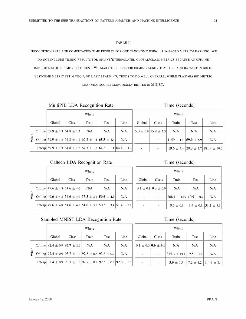
TABLE II

RECOGNITION RATE AND COMPUTATION TIME RESULTS FOR OUR TAXONOMY USING LDA-BASED METRIC-LEARNING. WE

DO NOT INCLUDE TIMING RESULTS FOR ONLINE/INTERPOLATED GLOBAL/CLASS METRICS BECAUSE AN OFFLINE

IMPLEMENTATION IS MORE EFFICIENT. WE MARK THE BEST-PERFORMING ALGORITHM FOR EACH DATASET IN BOLD.

TEST-TIME METRIC ESTIMATION, OR LAZY LEARNING, TENDS TO DO WELL OVERALL, WHILE CLASS-BASED METRIC

LEARNING SCORES MARGINALLY BETTER IN MNIST.

MultiPIE LDA Recognition Rate Time (seconds)

Where

Global Class Train Test Line

Whe

n

Offline 59.9 ± 1.3 64.8 ± 1.2 N/A N/A N/A

Online 59.9 ± 1.3 64.8 ± 1.2 62.2 ± 1.1 65.3 ± 1.4 N/A

Interp 59.9 ± 1.3 64.8 ± 1.2 64.3 ± 1.2 64.3 ± 1.1 64.4 ± 1.2

Where


5.0 ± 0.9 15.9 ± 2.5 N/A N/A N/A

- - 1159 ± 173 59.0 ± 5.9 N/A

- - 19.6 ± 3.4 28.3 ± 3.7 281.4 ± 40.0

Caltech LDA Recognition Rate Time (seconds)

Where


Whe

n

Offline 49.6 ± 4.8 54.6 ± 4.0 N/A N/A N/A

Online 49.6 ± 4.8 54.6 ± 4.0 55.5 ± 2.4 59.6 ± 4.9 N/A

Interp 49.6 ± 4.8 54.6 ± 4.0 51.6 ± 3.5 50.5 ± 3.4 51.4 ± 3.1

Where


0.1 ± 0.1 0.3 ± 0.0 N/A N/A N/A

- - 208.1 ± 12.9 10.9 ± 0.9 N/A

- - 0.6 ± 0.1 1.4 ± 0.1 31.1 ± 3.1

Sampled MNIST LDA Recognition Rate Time (seconds)

Where


Whe

n

Offline 92.4 ± 0.9 93.7 ± 1.0 N/A N/A N/A

Online 92.4 ± 0.9 93.7 ± 1.0 92.8 ± 0.8 93.6 ± 0.9 N/A

Interp 92.4 ± 0.9 93.7 ± 1.0 92.7 ± 0.7 92.5 ± 0.7 92.6 ± 0.7

Where


0.1 ± 0.0 0.6 ± 0.1 N/A N/A N/A

- - 375.3 ± 19.1 19.5 ± 1.4 N/A

- - 3.9 ± 0.5 7.2 ± 1.2 114.7 ± 8.4



TABLE III

RECOGNITION RATE AND COMPUTATION TIME RESULTS FOR ALL VARIANTS OF OUR TAXONOMY FOR THE

METRIC-LEARNING APPROACH. TEST-TIME METRIC ESTIMATION, OR LAZY LEARNING, DOES NOT DO WELL BECAUSE

METRIC-LEARNING TENDS TO OVERFIT. IN THIS CASE, AN ONLINE IMPLEMENTATION OF PER-EXEMPLAR TENDS TO

PERFORM WELL, WHILE PER-CLASS AGAIN DOES WELL ON MNIST. WE SHOW THAT OUR HYRBRID ALGORITHM

OUTPERFORMS THESE RESULTS IN TABLE IV.

MultiPIE Metric Learning Recognition Rate Time (seconds)

Where


Whe

n

Offline 59.2 ± 1.9 60.2 ± 1.8 N/A N/A N/A

Online 59.2 ± 1.9 60.2 ± 1.8 68.8 ± 1.3 61.2 ± 1.5 N/A

Interp 59.2 ± 1.9 60.2 ± 1.8 66.2 ± 1.5 66.1 ± 1.5 66.1 ± 1.6

Where


3.6 ± 0.3 12.9 ± 0.6 N/A N/A N/A

- - 1222 ± 9 1175 ± 32 N/A

- - 14.6 ± 0.8 22.4 ± 0.9 184.6 ± 8.7

Caltech Metric Learning Recognition Rate Time (seconds)

Where


Whe

n

Offline 51.1 ± 4.7 51.7 ± 3.7 N/A N/A N/A

Online 51.1 ± 4.7 51.7 ± 3.7 58.2 ± 3.1 53.7 ± 4.0 N/A

Interp 51.1 ± 4.7 51.7 ± 3.7 53.6 ± 4.4 53.7 ± 4.4 53.8 ± 4.5

Where


0.1 ± 0.0 0.3 ± 0.0 N/A N/A N/A

- - 222.4 ± 26.2 256.7 ± 16.3 N/A

- - 0.8 ± 0.2 1.7 ± 0.1 39.9 ± 6.8

Sampled MNIST Metric Learning Recognition Rate Time (seconds)

Where


Whe

n

Offline 92.4 ± 1.2 94.4 ± 0.8 N/A N/A N/A

Online 92.4 ± 1.2 94.4 ± 0.8 92.8 ± 0.7 93.1 ± 1.2 N/A

Interp 92.4 ± 1.2 94.4 ± 0.8 93.5 ± 0.8 93.5 ± 0.8 93.5 ± 0.8

Where


0.1 ± 0.0 0.6 ± 0.0 N/A N/A N/A

- - 310.2 ± 3.7 672.3 ± 15.4 N/A

- - 3.0 ± 0.0 5.2 ± 0.1 98.1 ± 0.9



TABLE IV

RECOGNITION RATE AND COMPUTATION TIME RESULTS FOR ALL VARIANTS OF THE HYBRID ALGORITHM

(SECTION II-B.3.) OVERALL, ONLINE ESTIMATION OF THE METRIC TENSOR AT THE TEST POINT IN OUR HYBRID

FRAMEWORK TENDED TO PERFORM THE BEST ACROSS TABLES II-IV. PER-CLASS PERFORMED BEST FOR MNIST,

CONSISTENT WITH PREVIOUS REPORTED RESULTS [24].

MultiPIE Hybrid Recognition Rate Time (seconds)

Where


Whe

n

Offline 59.2 ± 1.9 65.6 ± 1.4 N/A N/A N/A

Online 59.2 ± 1.9 65.6 ± 1.4 68.9 ± 1.2 70.2 ± 1.4 N/A

Interp 59.2 ± 1.9 65.6 ± 1.4 65.4 ± 1.5 65.4 ± 1.5 65.4 ± 1.5

Where


3.5 ± 0.0 12.6 ± 0.1 N/A N/A N/A

- - 1219 ± 12 63.3 ± 0.4 N/A

- - 14.3 ± 0.2 22.0 ± 0.1 184.5 ± 1.6

Caltech Hybrid Recognition Rate Time (seconds)

Where


Whe

n

Offline 51.1 ± 4.7 55.2 ± 4.9 N/A N/A N/A

Online 51.1 ± 4.7 55.2 ± 4.9 58.3 ± 3.2 60.1 ± 4.2 N/A

Interp 51.1 ± 4.7 55.2 ± 4.9 53.0 ± 4.0 52.0 ± 3.9 52.6 ± 4.3

Where


0.1 ± 0.0 0.3 ± 0.0 N/A N/A N/A

- - 223.7 ± 29.0 11.3 ± 1.3 N/A

- - 0.7 ± 0.0 1.6 ± 0.1 40.3 ± 6.9

Sampled MNIST Hybrid Recognition Rate Time (seconds)

Where


Whe

n

Offline 92.4 ± 1.2 93.8 ± 0.9 N/A N/A N/A

Online 92.4 ± 1.2 93.8 ± 0.9 92.9 ± 0.8 93.7 ± 0.8 N/A

Interp 92.4 ± 1.2 93.8 ± 0.9 92.6 ± 0.7 92.5 ± 0.7 92.6 ± 0.8

Where


0.1 ± 0.0 0.5 ± 0.0 N/A N/A N/A

- - 311.1 ± 3.1 15.7 ± 0.5 N/A

- - 3.1 ± 0.2 5.3 ± 0.2 97.8 ± 1.6


Documents

Local Distance Functions: A Taxonomy, New Algorithms, …€¦SUBMITTED TO THE IEEE TRANSACTIONS ON PATTERN ANALYSIS AND MACHINE INTELLIGENCE 1 Local Distance Functions: A Taxonomy,