Neurocomputing 430 (2021) 82–93

Contents lists available at ScienceDirect

Neurocomputing

journal homepage: www.elsevier .com/locate /neucom

Local-binarized very deep residual network for visual categorization

https://doi.org/10.1016/j.neucom.2020.11.0410925-2312/� 2020 Elsevier B.V. All rights reserved.

⇑ Corresponding author.E-mail address: liang.li@ict.ac.cn (L. Li).

1 This work was supported in part by the National Key R&D Program of China underGrant 2018YFE0303104, in part by National Natural Science Foundation of China:61732007, 61771457.

Xuejing Liu a,b,1, Liang Li a,⇑, Shuhui Wang a, Zheng-Jun Zha c, Qingming Huang a,b

aKey Laboratory of Intelligent Information Processing of Chinese Academy of Sciences (CAS), Institute of Computing Technology, CAS, Beijing 100190, Chinab School of Computer and Control Engineering, University of Chinese Academy of Sciences, Beijing 100190, Chinac School of Information Science and Technology, University of Science and Technology of China, Hefei 230027, China

a r t i c l e i n f o

Article history:Received 23 December 2019Revised 23 June 2020Accepted 19 November 2020Available online 2 December 2020Communicated by Cheng Jun

Keywords:Network compression and accelerationPose estimationObject recognitionSaliency detectionLocal binary residual block

a b s t r a c t

Residual networks usually require more layers to achieve remarkable performance in complex visual cat-egorization tasks, such as pose estimation. However, the increasing number of layers leads to a heavyburden on training and forward inference as well as over-fitting. This paper proposed local binary resid-ual block (LBB) to promote the very deep residual networks on the trainable parameters, FLOPs and accu-racy. In each LBB, the 3� 3 filters are binarized based on Bernoulli distribution under a sparse constraint,an activation function is prepared to trigger the non-linear response, and the linear 1� 1 filters arelearned in a real-valued way. After stochastic binarized initialization, the 3� 3 filters in LBB need notbe updated during training. The above architecture reduces at least 69.2% trainable parameters and70.5% FLOPs compared to the original model. The LBB is derived from three observations: 1) Activatedresponses of one standard k� k convolutional layer can be approximated by combining binarized k� kfilters with 1� 1 filters; 2) Most computation in the very deep residual networks is spent on the 3� 3convolutions; and 3) 1� 1 filters play an important role in cross-channel information integration. In addi-tion, the LBB module is suitable for the very deep network framework, including stacked hourglass net-work and pyramid residual modules. Experiments are conducted on MPII and LSP dataset for poseestimation task; CIFAR-10, CIFAR-100 and ImageNet datasets for object recognition; ECSSD, HKU-IS,PASCAL-S, DUT-OMRON, DUTS for saliency detection. The results show that our model can acceleratethe training and inference of the network with only a slight performance degradation.

� 2020 Elsevier B.V. All rights reserved.

1. Introduction

Deep Residual Networks (ResNets) [1] have achieved state-of-the-art results in object detection [2] and localization [3]. In spiteof the successes, ResNets require large amounts of memory andcomputational power for training due to the ever-increasing num-ber of convolutional layers. In addition, ResNets show its impres-sive accuracy on many complex visual categorization tasks, suchas human pose estimation [3,4].

To overcome the difficulties on pose estimation (occlusion,deformation, changes in clothing, lighting and camera views), themodified ResNets [3,5] can be up to 1000 layers, with a hugeincrease in the number of parameters and convolution operationscompared to ordinary ResNets for classification. Such giant-scalenetwork structures lead to a large number of training parameters,

large time consumption and more data requirement for modeltraining.

Along with the very deep networks, the need for inferencespeed-up is becoming urgent for real applications. For example, alightweight and compact binary architecture [6] is designed byremoving all the 1� 1 convolutional filters for landmark localiza-tion. Experiments show that network parameter binarizationgreatly accelerates the inference time by replacing most arithmeticoperations with bit-wise operations. However, compared withstandard real-valued networks, the performance of such binarizednetwork drops almost 12%, which is quite a large margin.

In deep networks, convolutional filters with different sizes cap-ture different patterns in data. There are two main kinds of filters.First, Spatial Convolution, such as 3� 3 or 5� 5, has a receptivefield capable of capturing locally spatial information. Its outputsindicate the response of the corresponding spatial patterns. Itspends most computation sources on learning this kind of filterfor generating more scalable spatial patterns. When the neural net-works achieve very deep architecture with 1000 + layers, there area large number of spatial filters. Even if our filters are randomlygenerated, the aggregation of responses from these filters can still

X. Liu, L. Li, S. Wang et al. Neurocomputing 430 (2021) 82–93

characterize rich and discriminant spatial patterns. Second, 1� 1Convolution filters are created for three purposes, 1) cross-channel information integration of feature maps from a givenlayer; 2) dimension reduction in the filter space; 3) increasingnon-linear activation layer like ReLU. A number of models acceler-ate the computation of the network by removing or binarizing the1� 1 filters. However, this has an adverse and irrecoverable influ-ence on the whole network.

To reduce the deep model training complexity, we proposedLocal Binary Residual Block (LBB), which is the basic module for verydeep networks. In LBB, 3� 3 spatial convolution filters are bina-rized, while 1� 1 convolution filters are learned in real values. Dif-ferent from existing work, the 3� 3 filters in LBB are stochasticallybinarized under a sparse constraint of Bernoulli distribution, andsuch constraint brings rich spatial patterns to the filters. Further-more, the LBB obtain an enormous amount of more discriminantspatial patterns by incrementally stacking the filters from differentlayers of very deep networks. In detail, weights of 3� 3 filters inLBB only need to be initialized in the above way and do not needto be updated during training. Thus it reduced at least 69.2% train-able parameters for a 1000-layered ResNet due to the sparsity ofbinary filters, and it accelerated the whole training and inferencestage because the binarized convolution operations are trans-formed into addition and subtraction operations. Besides, theexperiments show the different initializations of 3� 3 filters withBernoulli distribution bring a slight fluctuation of performance.

The combination of 1� 1 filters with binarized 3� 3 filterresponses aims to formulate the activated filter responses of onestandard 3� 3 convolutional layer. LBB can be seen as approximat-ing the full-precision weight with the linear combination of binaryweight bases. As Fig. 1b and Fig. 1c show, LBB is embedded intotwo different network blocks. One is the original block of stackedhourglass network (SHN), the other is the multi-branch pyramidresidual module (PRM), and they are generally called Local-Binarized Residual Networks (LBRN). Due to its sparsity, LBRN can1) save computations; 2) reduce the model size, both in terms ofmemory usage and disk space; 3) avoid overfitting. During infer-ence, the convolution operation in 3� 3 filters turns into judgmentwhether the information should be transferred or not to the nextlayer. It defines a new kind of convolution operation, which cansignificantly accelerate the forward propagation process.

The main contributions can be summarized as,

� We proposed local binary residual blocks (LBB) for acceleratingthe training and inference of very deep residual networks. LBBcan be embedded in residual networks without bells and whis-

Fig. 1. The residual block structures of different ResNets. (a) The original bottleneck blockstructure of our LBB in stacked hourglass network. Only the 3� 3 convolutions are biconvolutions are binarized. Note: a rectangular block containing: batch normalization, a

83

tles. Promising results are obtained on the complex task,namely pose estimation, which indicates that it is not necessaryto train all the parameters in the very deep networks.

� The spatial convolution filters in LBB are generated throughstochastic binarization under a sparse constraint of Bernoullidistribution, whose weights do not need to be updated duringtraining. This reduces at least 69.2% trainable parameters for a1000-layered deep residual network. At inference time, theFLOPs of each block in LBRN is 0.5 GFLOPs while that of thefull-precision network is 1.7 GFLOPs.

� Experiments show the LBB provides acceleration for the verydeep network with only a small performance degradation. Theperformance is getting better as the number of layers and chan-nels in 1� 1 filters increases. The performance of the whole net-work is insensitive to the sparsity level setting of binary spatialfilters.

The rest of the paper is organized as follows. Section 2 presentsrelated work on network compression and acceleration, especiallybinarization, and pose estimation. Section 3 introduces the method-ology of our proposed LBB, and more technical details, such as thebinarization method and network structure. Section 4 shows thequantitative experiments about our LBRN and their correspondinganalysis. Section 5 draws the conclusions.

2. Related work

2.1. Binarization

A significant number of approaches [7–11] has been promptedto reduce the storage and computation costs of convolutional neu-ral networks recently. These methods can be categorized into fourdirections: network pruning [12–14], network quantization [15–17], knowledge distillation [18–20] and compact network [21–23]. Particularly, binarization is a special case of quantization.Low precision binary network can save a lot of storage for DNNs.Besides, binary networks can only perform bit operations, whichcan greatly decrease the time consuming of DNNs. Thus approxi-mating real-valued weights with binary representations hasattracted much attention from researchers.

M. Courbariaux et al. introduce Binarized Neural Networks(BNNs), whose weights and activations is binarized at run-time.Thus the memory size and computation consuming are greatlydecreased. Furthermore, it achieves almost the same performanceof state-of-the-art results on several datasets [24]. M. Rastegariet al. propose two efficient networks: Binary-Weight-Networks

of stacked hourglass networks. The parameters of the blocks are real-valued. (b) Thenarized. (c) The structure of our LBB in pyramid residual module. Only the 3� 3ctivation function, filter size, data type, the number of input and output channels.

X. Liu, L. Li, S. Wang et al. Neurocomputing 430 (2021) 82–93

and XNOR-Networks. Both the filters and input are binarize inXNOR, resulting in 58� faster convolutional operations and 32 �memory saving [25].

Based on XNOR, A. Bulat et al. design a lightweight, compactand suitable multi-scale residual network for landmark localiza-tion, which is the first work to apply binarization on landmarklocalization tasks [6]. F. Juefei-Xu et al. propose local binary convo-lutions, which couple pre-defined binary filters with learnable lin-ear weights for classification [26]. Z. Li et al. introduce a high-orderbinarization scheme, which recursively performs residual quanti-zation and got high-order binary filters and gradients. The recur-sive binarization operation can approximate the original networkmore accurately. [27]. X. Lin et al. propose ABC-Net, which is differ-ent from preceding networks in two aspects. Firstly, it approxi-mates the full-precision weight with the linear combination ofseveral binary weight bases. Secondly, it utilizes multiple binaryactivations to decrease information loss. ABC-Net achieves compa-rable results as full-precision networks [28]. A. Mishra and D. Marrimprove the performance of low-precision networks throughknowledge distillation. This approach is called Apprentice, whichhas three schemes and achieves state-of-the-art accuracy usingternary precision [29].

2.2. Pose estimation

A. Bulat and G. Tzimiropoulos design a detection-followed-by-regression CNN cascaded architecture to learn part relationshipand spatial information, which is robust even for severe part occlu-sions [30]. SE. Wei et al. incorporate convolutional networks intopose machine framework to learn image features and image-dependent spatial models for pose estimation. They address theproblem of vanishing gradients through intermediate supervisionand get admirable results on several important benchmarks [31].Z. Cao et al. propose a bottom-up parsing architecture to detect2D pose of multiple people in an image, which achieves real-timehigh accuracy. This approach uses Part Affinity Fields, which is anon-parametric representation, to associate body parts in individ-uals. Their method exceeds previous results on MPII benchmarkboth in performance and efficiency [4]. Y. Chen et al. propose astructure-aware convolutional network, which incorporates priorknowledge of human bodies. They design discriminators to distin-guish the real pose and the fake pose generated by pose generatorto learn the priors successfully. Their approach outperforms theprevious method and generates plausible human posed [32].

The very deep residual neural networks have achieved someremarkable results in many tasks, but they bring a huge burdenon computation resources and have a huge number of parameters,which makes the networks difficult to train and slow to converge.Our model aims at optimizing the architecture of very deep neuralnetworks for pose estimation with our local binary residual blocks(LBB), which can accelerate the procedure of network learningwhile keeping a slight performance degradation. We apply ourLBB in two different networks for pose estimation: stacked hour-glass network [3] and pyramid residual module [33]. Actually,our model can be easy to extend into any deep network structures.As each hourglass is a repeated bottom-up, top-down processingwith intermediate supervision, it demands quite large computationresources. Our method is essentially a kind of trade-off betweenaccuracy and time efficiency.

3. Methodology

In this section, we first introduce stacked hourglass network,pyramid residual modules, and local binary pattern. Stacked hour-glass network is a widely used network for pose estimation with a

84

repeated bottom-up, top-down structure. Pyramid residual mod-ules aim to enhance the ability for multi-scale feature extractionof stacked hourglass network. Based on the two networks, we uti-lize local binary residual block (LBB) for pose estimation and getsatisfying performance. Then we demonstrate how we apply LBBto the networks for pose estimation and the whole network struc-ture. Next, we introduce two different binarization method and thereason why we use the stochastic binarization method under asparse constraint in LBB. In the end, we formulate LBB and explainwhy it can decrease the inference and training time.

3.1. Stacked hourglass network

Stacked hourglass network (SHN) is proposed by Newell et al.[3], which is a widely used network for pose estimation. Due tothe flexibility of poses and different points of view, the scale of dif-ferent body parts in each image are changed tremendously. Themotivation of SHN is to capture information of the image at everyscale. The hourglass network fuses all the features together to out-put pixel-wise predictions.

SHN is a repeated bottom-up, top-down processing with anintermediate supervision structure, as shown in Fig. 2. The stepsof pooling and subsequent is vital to combine features across allscales and capture multiple spatial relationships with the body,thus improving the performance of the network, and intermediatesupervision is crucial for the network to get the considerable per-formance. Overall, their network shows robust results on MPII andFLIC benchmarks and outcompeting all the past methods.

3.2. Pyramid residual modules

The difficulty of pose estimation lies in scale variations of differ-ent parts due to camera view change and foreshortening. Althoughthe structure of SHN can capture information of an image at everyscale with its repeated bottom-up, top-down structure, in eachblock the SHN can only capture features at one scale. Thus Yanget al. propose pyramid residual modules (PRM) [33] to enhancethe network’s ability for scale variations. Each block in PRM is amulti-branch structure, as can be seen in Fig. 1c. The pyramidresidual module is to build feature pyramids.

Yang et al. proposed four different kinds of pyramid residualmodules to capture multi-scale features in an image. Our basedmodel is shown in Fig. 1c. To capture multi-scale visual patternsor semantics, the convolutional network turns into multi-branch.The left branch is an identity mapping. The middle branch is thesame structure as the block in SHN. The branch on the right is sep-arated into multi-branches again. Each branch has filters with dif-ferent subsampling ratios. To reduce the resolution slowly andsubtly, fractional max-pooling [34] is adopted to resize the featuremaps. The computation of fractional max-pooling is shown asfollows:

sc ¼ 2�McC ;dffc ¼ 0; . . . ;C;M P 1; ð1Þ

where sc denotes the subsampling ratio between the output fea-tures and input features, which ranges from 2�M to 1. c denotesthe cth level. For example, when c ¼ 0, the resolution does notchange. When M ¼ 1; c ¼ C, the subsampling ration is 1

2.

3.3. Network structure

Although SHN and PRM get remarkable results on pose estima-tion, the repeated residual blocks are quite a burden for trainingand testing. Taking SHN as an example, the number of its layersis up to 1464, which requires a large amount of computation andmemory resources.

Fig. 2. The architecture of our LBRN under the structure of stacked hourglass networks, which stacks 8 hourglasses block. Each hourglass is composed of successive steps ofpooling and upsampling. LBB is our designed local-binarized residual block, which is the core component block of LBRN.

X. Liu, L. Li, S. Wang et al. Neurocomputing 430 (2021) 82–93

To reduce time and memory consumption of residual networksfor pose estimation, [6] proposed a full binarized residual network.The final block structure is a novel hierarchical, parallel, and multi-scale residual architecture, which is more suitable for binarization.Its binarization method is deterministic on the base of Binary-Weight-Network [25]. However, the performance of full binarizedresidual networks degrades significantly. In addition, a carefullydesigned residual block is vital to get better performance, whichmakes it less flexible to adapt to existing ResNets [1].

To alleviate the above problems, as illustrated in Fig. 2, we pro-pose local binary residual block (LBB). In LBB, only the 3� 3 filtersare binarized under a sparse constraint while the 1� 1 filtersremain real-valued. The motivations of LBB stem from threeaspects, 1) activated responses of one standard k� k convolutionallayer can be approximated by 1� 1 filters with binarized filterresponses; 2) most computation in the very deep residual net-works concentrates on the 3� 3 convolutions; 3) 1� 1 filters playan important part in cross-channel information integration.

LBB can be embedded in the structure of stacked hourglass net-work and pyramid residual module easily. As shown in Fig. 1a andb, LBB is able to keep the consistent structure as the original bottle-neck of SHN. Fig. 1c shows the application of LBB to PRM, whichdoesn’t change any of the original settings. LBB can be applied toresidual networks without any bells and whistles. These residualnetworks with LBB for pose estimation are called LBRN for conve-nience in the subsequent.

As can be seen in Fig. 1b and c, the batch normalization andactivation function precede a convolutional layer in LBB. All the3� 3 filters are binarized under a sparse constraint. Besides, inview of the effectiveness of the successive step of pooling andupsampling in SHN, the two LBRNs keep a similar design philoso-phy to it. At last, LBRNs produce a final set of heatmaps forprediction.

85

At the training stage, the weights of binarized filters do notneed to be updated, so that there is no need to calculate the gradi-ents in the 3� 3 convolutional layers. For the original SHN, it cansave at least 69.2% trainable parameters. For the task where filterswith larger size are needed, LBRN help to reduce more trainableparameters. Taking 5� 5 filters as an example, it can save 86.2%parameters during the training step. In testing, since the weightsare binary, the convolution operations can be performed purelythrough additions and subtractions.

3.4. Binarization

In this subsection, we explore the binarization method in ourlocal binary residual block (LBB) for better and faster processing.

Generally, two different binarization approaches are usuallyused in neural networks nowadays. One is deterministic methodsas follows,

sign ðxÞ ¼þ1 x P 0;�1 x < 0;

8><>:

ð2Þ

The above sign function is a typical representation, where x denotesa real-valued variable. Based on this straightforward and intuitivefunction, several works have been proposed [35,25,28] to approxi-mate the real-valued weights with binary weights.

However, shift-based batch normalization and specific updatingrules of weights such as discretization of gradients and optimiza-tion methods are carefully designed in the deterministic binariza-tion method. Furthermore, the weights are updated repeatedlyduring the whole training process, which needs a lot of trainingtime.

X. Liu, L. Li, S. Wang et al. Neurocomputing 430 (2021) 82–93

The other one is the stochastic method, which requires thehardware to generate random bits to imitate the real-valuedweights. It has two impressive advantages, 1) it is easy to imple-ment as no specific updating rules are needed compared to deter-ministic ones 2) the binary weights need not be updated during thetraining stage once they are generated. These binarized layers arevery similar to ReLU or Max Pooling layers, which do not haveany learnable parameters. [26] applied randomly generated binaryweights to standard convolutional neural networks (CNNs) andachieved performance comparable to regular CNNs on the task ofclassification. Considering the simplicity and efficiency, we designour LBB in the stochastic binarization method under a sparseconstraint.

The procedure of stochastic binarization under a sparse con-straint is as follows. First, a sparsity level is needed consideringthe tolerance of the weights to non-zero values. The sparsity levelis set as 0.5 here, which means half of the parameters are zero. Sec-ond, the rest parameters are assigned to + 1 or �1 randomly withequal probability, according to Bernoulli distribution. The Bernoullirandom vectors are subgaussian and isotropic, which ensures thatactivated responses of one standard k� k convolutional layer canbe approximated by 1� 1 filters with binarized filter responsesand more intermediate binary filters can result in a better approx-imation. Fig. 3 presents some examples of our binary convolutions.

3.5. Efficiency analysis

In this subsection, we take LBB based on stacked hourglass net-work as an example to explain why it can reduce trainable param-eters and accelerate training and testing steps.

3.5.1. Residual ModuleAs Fig. 1b shows, LBB in an hourglass consists of three parts. For

each residual module, let Xl;Xlþ12 Rc�w�h be the input and the out-put, where ðc;w;hÞ represents channels, width, height respectively.let the intermediate results be denoted by Xm1;Xm2 2 Rcm�w�h.

W1 2 Rc�1�1�cm ;Wb 2 f0;�1gcm�3�3�cm ;W2 2 Rcm�1�1�c representthe weights of these three different parts respectively, where themiddle two dimensions are filter size and the other two are inputand output channels. The forward procedure of LBB can be com-puted as follows:

Xm1 ¼ rreluðXlÞ �W1;

Xm2 ¼ rreluðXm1Þ �Wb;

Xlþ1 ¼ rreluðXm2Þ �W2 þ Xl;

8><>:

ð3Þ

where � denotes convolution operation, � indicates a convolutionwithout any multiplication, W1;W2 denotes real-valued weight,Wb indicates the binarized weights. The weights of 3� 3 filtersare binary thus we only need additions and subtractions.

3.5.2. Parameter SavingThe learnable parameters are greatly reduced as the 3� 3 filters

do not need to be updated during training. As we can see, the num-

Fig. 3. Examples of our binary convolutions.

86

ber of trainable parameters in original real-valued residual blockcan be computed as follows:

Pr ¼ c � cm þ cm � 3� 3� cm þ cm � c: ð4ÞThe number of trainable parameters in LBB is as follows:

Pb ¼ c � cm þ cm � c: ð5ÞThe ratio of the parameters of these two blocks is

PrPb

¼ c�cmþcm�3�3�cmþcm�cc�cmþcm�c

¼ 1þ 92 � cm

c :ð6Þ

In our paper, cm is usually half of c. So the ratio equals to 3.25. If weenlarge the filter size, for example, from 3� 3 to 5� 5, the ratio willbe 7.25.

3.5.3. Computation efficiencyWe compare the computation efficiency of LBB and real-valued

residual block through floating point operations (FLOPs). The com-putation of FLOPs we used in our paper is the same as [36]. Convo-lution is regarded as a sliding window and the nonlinearityfunction is computed for free. Thus, the computation formulationis:

FLOPs ¼ 2HWðCinK2 þ 1ÞCout; ð7Þ

where H and W are height and width, K is the kernal size andCin;Cout denote the number of input and output channels.

Here, we omit the bias. Thus, for a real-valued residual block instacked hourglass network the FLOPs is:

FLOPsr ¼ 2� 2� 64� 64� 256� 1� 1� 128þ 2� 64� 64

� 128� 3� 3� 128

� 1:7GFLOPs; ð8Þ

For our LBB we compute FLOPs as:

FLOPsb ¼ 2� 2� 64� 64� 256� 1� 1� 128� 0:5GFLOPs;

ð9Þ

so LBRN can be about 3� faster than original real-valued networks.

3.6. Convergence analysis

Here is the proof why any 3� 3 convolution can be approxi-mated by 3� 3 binary filter with 1� 1 filters. Suppose X is the fea-ture maps of input layer, B is the fixed binary 3� 3�M � P filters,V is the 1� 1� P � N filters, W is 3� 3�M � N filters, M is thechannel number of input layer, N is that of output layer, P is thatof intermediate output). Our goal is to prove

C � B ð10Þwhen

C ¼ rreluðWTXÞ;B ¼ DTV ;

DrreluðBXÞ:ð11Þ

There are two cases. 1) C ¼ 0: because D >¼ 0, there always exits aV such that C ¼ B. 2) C > 0: If D > 0, there exits a V such that C ¼ B.If D ¼ 0, the approximation does not hold. According to Theorem.5.39 in [37] and concentration inequalities, D vector are greaterthan zero with high probability. So any 3� 3 convolution can beapproximated by the cascading of 3� 3 binary filter and 1� 1filters.

X. Liu, L. Li, S. Wang et al. Neurocomputing 430 (2021) 82–93

4. Experiments

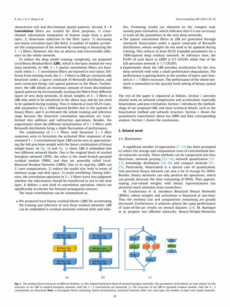
We conduct experiments on two widely used datasets forhuman pose estimation: MPII, LSP and its extended dataset LSPET.We use the same PCKh evaluation method for both datasets. Wetest the two different LBRNs and compare the results with the orig-inal full-precision networks. Some experiments are conducted toverify the importance of 1� 1 filters. Experiments on the sparsitylevel are presented. Ablation studies are provided to see the influ-ence of different settings. We also conduct experiments on CIFAR-10, CIFAR-100 datasets and ImageNet for object recognition andECSSD, HKU-IS, PASCAL-S, DUT-OMRON, DUTS for saliency detec-tion. The results show that our method is suitable for object recog-nition and saliency detection as well.

4.1. Pose estimation on MPII dataset

The MPII human pose dataset, which is made for articulatedhuman pose estimation [38]. It contains 25 K images over 40 Kpeople with annotated body joints (28 k training and 11 k testing).Each image is extracted from YouTube video on every day humanactivities. Since testing annotations are not provided, all the resultsare generated on the standard training-validation partition of MPII.The validation contains about 3000 samples.

4.1.1. Training SettingsThe LBRN based on stacked hourglass network (LBRN-S) is

trained through RMSprob [39] algorithm with a learning rate of2.5e-4, which can speed up first-order gradient descent methods.The training epoch is 100 with a mini-batch size of 4. Batch nor-malization operations are used before each convolutional layer,speeding up training and reducing the internal covariate shift ofinput data. The loss function is Mean Squared Error (MSE) criterionwhich minimizes the distance between prediction and target.Compared to the original stacked hourglass networks (SHN), theonly extra hyper-parameter is sparsity level, the percentage ofnon-zero values in the local-binarized convolutional layers. It isnotable that the weights of 3� 3 convolutions are fixed so thatthere is no need to calculate the gradients or update the weights.

Data augmentation method such as scaling, rotation, flipping isused at training step for both networks. The LBRN based on PRM(LBRN-P) uses the same optimization method as stacked hourglassnetwork. We train the PRM network with 2 stacked hourglasses.The training epoch is 250 with a mini-batch size of 6. The initial-ized learning rate is 2.5e-4 which is dropped by 10 at 150th,170th and 200th epoch. The cardinality is set as 4, which meansthe feature pyramids will be divided into four scales.

4.1.2. Evaluation MeasuresWe take advantage of the Percentage Correct Keypoints (PCK)

metric for evaluation. On MPII, PCKh metric, where the distanceis normalized based on head size of the target [38], is used in ourresults. PCKh@0.5 denotes the distance less than a normalized dis-tance of 0.5.

4.1.3. ResultsWe compare the LBRNs with real-valued ResNets, full-binarized

ResNets [6] and full-binarized stacked hourglass network on theMPII dataset. Full-binarized stacked hourglass network has thesame structure as our LBRN. Full-binarized ResNets [6] is a hierar-chical, parallel and multi-scale structure designed for pose estima-tion. Fig. 1a, Fig. 1b and Fig. 1c denote the bottleneck block ofstacked hourglass network, LBRN-S and LBRN-P respectively. Wecan see from the block structure that before each convolutionallayer (1� 1;3� 3), batch normalization and ReLU layer are

87

stacked. Both the LBRNs follow the structure of stacked hourglassas Fig. 2 shows. However, stacked hourglass network and its corre-sponding LBRN-S are built up with 8 hourglasses, while PRM andits corresponding LBRN-P have only 2 hourglasses. Table 1 presentsthe comparison results, and we can have the following findings.

First, comparing with full-binarized neural networks, LBRN-Sand LBRN-P achieve a significant improvement of 9.3% and 9.5%separately while the size of parameters is very close. This meansthat our local binary residual module can boost the performanceunder a low parameter growing. It is not necessary to train allthe parameters in a residual network for pose estimation.

Second, compared with SHN and PRM, LBRN-S and LBRN-P havea slight performance degradation of 1.4% and 0.8%, but the param-eter number of LBRN-S and LBRN-P is about 30% of SHN and PRM,which means LBRN can save plenty of parameter space and train-ing time. Furthermore, the 3� 3 filters do not need to be updatedduring the training stage, and this can accelerate the training of themodel. During inference time, the convolution operation in 3� 3filters turns into judgment whether the information should betransferred or not to the next layer. It defines a new kind of convo-lution operation, which can significantly accelerate the forwardpropagation process.

Third, due to the number of stacked hourglasses, the perfor-mance of PRM is less than SHN. However, the performance ofLBRN-P is better than LBRN-S. Perhaps it is because of the multi-scale structure of PRM, which corresponds to different scales oflocal binary pattern.

Fourth, Fig. 5 shows some examples of pose estimation fromthese networks. The pose estimation of our LBRN is very similarto that of real-valued networks. On the contrary, many defectsappear on the results of full-binarized residual networks. In short,our LBB can be regarded as one substitute for traditional very deepneural networks.

4.1.4. Ablation StudyWe conducted experiments with different settings to find better

network structure and hyper-parameters.

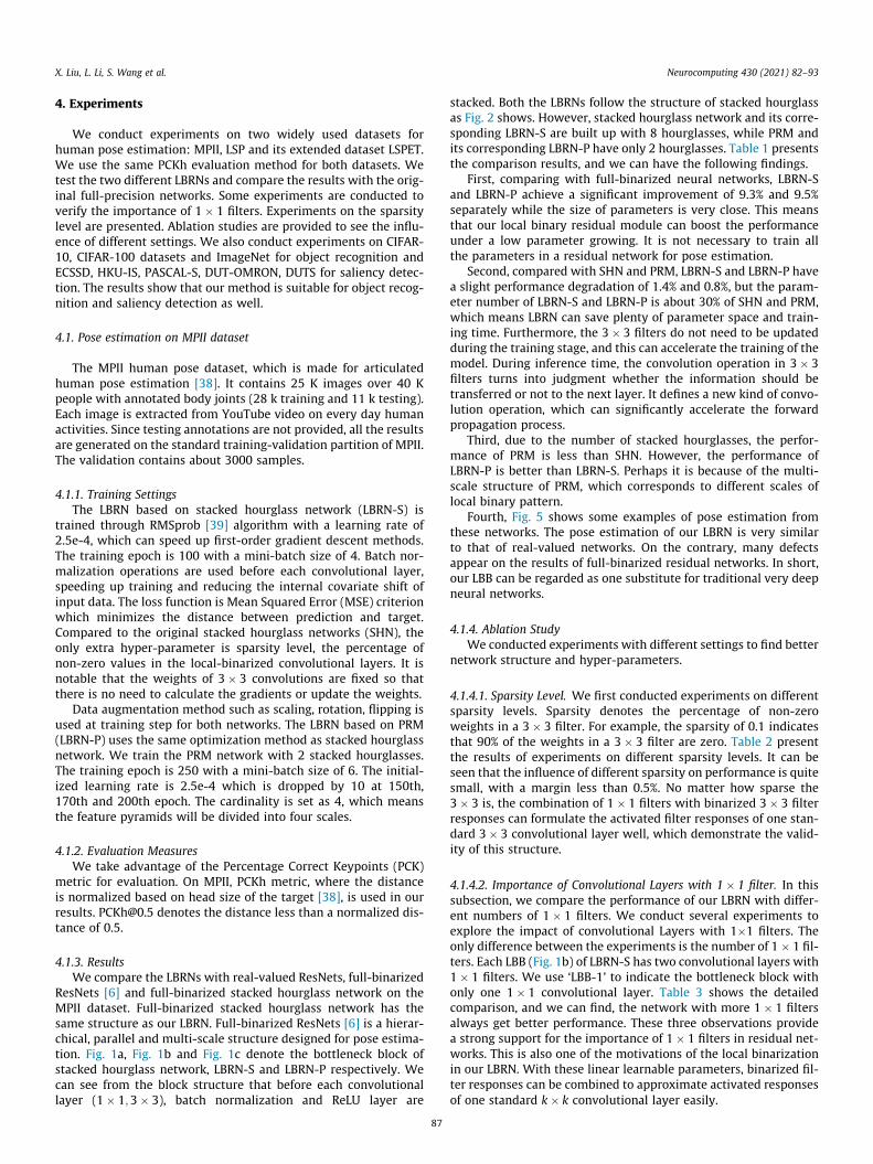
4.1.4.1. Sparsity Level. We first conducted experiments on differentsparsity levels. Sparsity denotes the percentage of non-zeroweights in a 3� 3 filter. For example, the sparsity of 0.1 indicatesthat 90% of the weights in a 3� 3 filter are zero. Table 2 presentthe results of experiments on different sparsity levels. It can beseen that the influence of different sparsity on performance is quitesmall, with a margin less than 0.5%. No matter how sparse the3� 3 is, the combination of 1� 1 filters with binarized 3� 3 filterresponses can formulate the activated filter responses of one stan-dard 3� 3 convolutional layer well, which demonstrate the valid-ity of this structure.

4.1.4.2. Importance of Convolutional Layers with 1� 1 filter. In thissubsection, we compare the performance of our LBRN with differ-ent numbers of 1� 1 filters. We conduct several experiments toexplore the impact of convolutional Layers with 1�1 filters. Theonly difference between the experiments is the number of 1� 1 fil-ters. Each LBB (Fig. 1b) of LBRN-S has two convolutional layers with1� 1 filters. We use ‘LBB-1’ to indicate the bottleneck block withonly one 1� 1 convolutional layer. Table 3 shows the detailedcomparison, and we can find, the network with more 1� 1 filtersalways get better performance. These three observations providea strong support for the importance of 1� 1 filters in residual net-works. This is also one of the motivations of the local binarizationin our LBRN. With these linear learnable parameters, binarized fil-ter responses can be combined to approximate activated responsesof one standard k� k convolutional layer easily.

Table 1Results on MPII validation set (PCKh@0.5). HG-Binary: Full-binarized stacked hourglass network [6]. Binary: Full-binarized residual network [6]. SHN: Stacked hourglass network.LBRN-S: Local-binarized residual network based on stacked hourglass network. PRM: Pyramid residual module network. LBRN-P: Local-binarized residual network based onpyramid residual module. #Param: The amount of trainable parameters of each basic residual block.The Binary, SHN, LBRN-S are bult up with 8 hourglasses, while PRM, LBRN-Pare built up with 2 hourglasses for efficiency. For LBRN-S on MPII dataset, the average PCKh over ten repetitions is 87.2+/-0.14.

HG-Binary Binary SHN LBRN-S PRM LBRN-P

Head 90.5 94.7 96.7 96.4 96.2 96.1Shoulder 79.6 89.6 95.0 94.0 95.2 95.1Elbow 63.0 78.8 88.2 87.5 89.2 88.2Wrist 57.2 71.5 84.3 81.4 84.3 82.6Hip 71.1 79.1 86.4 85.5 88.4 88.3Knee 58.2 70.5 84.4 80.5 83.6 82.7Ankle 53.4 64.0 80.7 77.0 80.6 79.2Total 67.2 78.1 88.8 87.4 88.4 87.6#Param 0.006 0.013 M 0.213 M 0.065 M 0.262 M 0.078 MFLOPs - - 1.7G 0.5G 2.1G 0.6G

Table 2Results on MPII validation set of different sparsity(PCKh@0.5).

Sparsity Elbow Wrist Knee Ankle Total

0.1 86.6 81.6 81.8 78.2 87.20.2 86.4 81.9 80.8 78.1 87.00.3 87.1 82.2 81.3 77.8 87.40.4 87.0 82.2 81.3 77.8 87.40.5 86.7 81.1 81.3 78.4 87.10.6 87.2 81.4 81.0 78.2 87.20.7 87.5 81.9 81.2 77.6 87.40.8 86.8 81.5 81.4 78.6 87.10.9 87.2 81.6 81.7 77.8 87.2

Table 3Results on MPII validation set (PCKh@0.5). The bold number denotes the number of 1� 1 filters of each convolutional layer. ‘LBRN’ here denotes the networks based on stackedhourglass network (LBRN-S). There is only 1 layer of 1� 1 filters in ‘LBRN-1’. The sparsity here is 0.5.

LBRN(256) LBRN(128) LBRN(64) LBRN-1(256)

Head 96.4 96.0 95.3 95.8Shoulder 94.0 93.7 92.5 92.9Elbow 87.5 86.0 83.1 84.5Wrist 81.4 80.1 76.6 78.2Hip 85.5 85.4 83.1 82.4Knee 80.5 80.5 76.6 77.8Ankle 77.0 76.5 72.8 74.4Total 87.1 86.5 84.1 84.8

Table 4Results on MPII validation set (PCKh@0.5). LBRN-1 denotes the network removing allthe 3� 3 filters. LBRN-2 denotes the network binarizing 1� 1 convolutional layerswhile keeping 3� 3 convolutional layers real-valued. LBRN-3 denotes the networkbinarizing half the filters in 3� 3 convolutional layers. The sparsity level here is 0.5.

LBRN-1 LBRN-2 LBRN-3

Head 79.3 96.0 96.5Shoulder 67.1 93.7 94.6Wrist 48.5 80.4 83.8Elbow 52.8 86.7 88.1Hip 44.3 84.8 86.5Knee 38.5 80.7 83.4Ankle 40.6 77.7 79.8Total 54.6 86.7 88.4

X. Liu, L. Li, S. Wang et al. Neurocomputing 430 (2021) 82–93

4.1.4.3. Network Structure. We conduct experiments on three dif-ferent network structure settings: 1) removing the 3� 3 filters,2) binarizing 1� 1 convolutional layers while keeping 3� 3 convo-lutional layers real-valued, 3) binarizing half the filters in 3� 3convolutional layers. Table 4 shows the results of the three differ-ent settings.

The total PCKh of LBRN-1 is 54.6%, which is far below the result(87.2%) of LBRN-S at sparsity level of 0.1. This is because 3� 3 bin-ary filters with a sparsity of 0.1 are different from 1� 1 filters, evenif there is only one activated element in a 3� 3 filter. To generateone feature map, we need a 3� 3� N filter. The combination of Nstacked 3� 3 filters corresponds to a larger receptive field than1� 1 filters. It can bring more discriminative representation.

Most parameters and computation resources are spent on 3� 3convolutional layers. Binarizing 1� 1 convolutional layers whilekeeping 3� 3 convolutional layers real-valued is weak in networkspeedup and compression. The total PCKh of LBRN-2 is 86:7% onMPII dataset, which is 0:7% lower than LBRN-S. Besides, It spends2:4� longer time and 2:66� memory than LBRN-S. The total PCKhof LBRN-3 is 88:4%, which is only 1% higher than LBRN-S. How-ever, It consumes 2:2� longer time and 2:1� memory thanLBRN-S.

88

4.1.4.4. Network size. Two kinds of experiments are conducted toverify the impact of different model sizes. One is to alter the num-ber of stacked hourglasses, the other one is to change the size ofthe hourglass module.

Table 5 shows the comparison results. We can observe, 1) net-works with 8 stacked hourglasses outperform the ones with 4,which is consistent with the conclusion of real-valued ones [3].2) the performance descents if the hourglass is halved, which

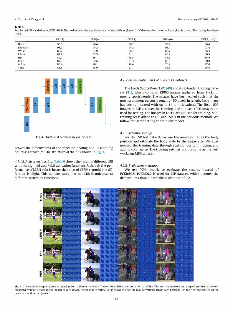
Table 5Results on MPII validation set (PCKh@0.5). The bold number denotes the number of stacked hourglasses. ‘half’ denotes the structure of hourglass is halved. The sparsity level hereis 0.5.

SHN(8) SHN(4) LBRN(8) LBRN(4) LBRN(8, half)

Head 96.6 96.4 96.2 95.7 96.4Shoulder 95.2 94.2 94.2 93.4 93.4Wrist 88.7 87.9 86.7 85.7 86.4Elbow 84.1 82.9 81.1 80.2 80.9Hip 87.0 86.1 85.5 85.3 85.0Knee 83.6 82.6 81.3 80.8 80.0Ankle 80.4 80.1 78.4 76.9 77.6Total 88.8 88.0 87.1 86.5 86.6

Fig. 4. Structure of halved hourglass (hg-half).

X. Liu, L. Li, S. Wang et al. Neurocomputing 430 (2021) 82–93

proves the effectiveness of the repeated pooling and upsamplinghourglass structure. The structure of ‘half’ is shown in Fig. 4.

4.1.4.5. Activation function. Table 6 shows the result of different LBBwith the sigmoid and ReLU activation functions Although the per-formance of LBRN-relu is better than that of LBRN-sigmoid, the dif-ference is slight. This demonstrates that our LBB is universal todifferent activation functions.

Fig. 5. The example output of pose estimation from different networks. The results of LBbinarized residual networks. On the left of each image, the final pose estimation is provheatmaps of different joints.

89

4.2. Pose estimation on LSP and LSPET datasets

The Leeds Sports Pose (LSP) [40] and its extended training data-set [41], which contains 12000 images gathered from Flickr ofmostly sportspeople. The images have been scaled such that themost prominent person is roughly 150 pixels in length. Each imagehas been annotated with up to 14 joint locations. The first 1000images in LSP are used for training, and the last 1000 images areused for testing. The images in LSPET are all used for training. MPIItraining set is added to LSP and LSPET in the previous method. Wefollow the same setting to train our model.

4.2.1. Training settingsFor the LSP test dataset, we use the image center as the body

position and estimate the body scale by the image size. We aug-mented the training data through scaling, rotation, flipping, andadding color noise. The training settings are the same as the net-works on MPII dataset.

4.2.2. Evaluation measuresWe use PCKh metric to evaluate the results. Instead of

PCKh@0.5, PCKh@0.2 is used for LSP dataset, which denotes thedistance less than a normalized distance of 0.2.

RN are similar to that of the full-precision network and outperform that of the full-ided after the max activations across each heatmap. On the right we can see all the

Table 6The performance comparison of the LBRN-S with different activation functions. Thesparsity level here is 0.5.

LBRN-relu LBRN-sigmoid

Head 96.2 96.0Shoulder 94.2 93.3Elbow 86.7 86.1Wrist 81.1 82.0Hip 85.5 84.7Knee 81.3 81.2Ankle 78.4 77.4Total 87.1 86.7

X. Liu, L. Li, S. Wang et al. Neurocomputing 430 (2021) 82–93

4.2.3. ResultsThe results of SHN, PRM and LBRN on LSP dataset are shown in

Table 7. For SHN and LBRN-S, we stacked 8 hourglasses for trainingand testing, while PRM and LBRN-P are built up with 2 hourglassesfor efficiency. That’s the reason why SHN performs better thanPRM. The results of SHN is 1.5% higher than LBRN-S and that ofPRM is only 0.6% higher than LBRN-P. Similar to the results on MPIIdataset, the margin between SHN and LBRN-S is larger than that ofPRM and LBRN-P. This is corresponding to the characteristic oflocal binary pattern (LBP). It can meet the needs of capturing fea-tures of large scale structures when the LBP is multi-scale. Fig. 6shows some examples and failure cases of the network output onLSP dataset.

4.2.4. Sparsity levelTable 2 shows different sparsity levels of LBRN-S have little

impact on the performance for MPII dataset. We also conductexperiments of LBRN-P with different sparsity on LSP dataset.

Fig. 6. Some example output of the different networks on LSP dataset. Some failure cases

Table 7The performance comparison(PCKh@0.2). SHN: Stacked hoLocal-binarized residual netwoglass network. PRM: PyramidLBRN-P: Local-binarized residuamid residual module. The SHN,hourglasses, while PRM, LBRNhourglasses for efficiency. Theand LBRN-P is 0.5. For LBRN-P oPCKh over ten repetitions is 91

SHN LBRN

Head 98.5 97.7Shoulder 94.6 93.6Elbow 90.2 88.7Wrist 87.6 85.1Hip 94.2 92.8Knee 94.0 92.4Ankle 93.5 91.5Total 93.2 91.7

90

Table 8 shows the results. The same observation is obtained thatthe sparsity level has little impact on the performance, so we canchoose the sparsity level according to the computing power ofthe hardware device. The representation ability of LBB dependson cascading binary 3� 3 filters and 1� 1 filters. It achieves theoptima by learning the 1� 1 filters in the training stage.

4.3. Object recognition on CIFAR datasets and ImageNet

The CIFAR Dataset [42], including CIFAR-10 and CIFAR-100, is awidely used dataset for object recognition. The CIFAR-10 datasetconsists of 50000 training images and 10000 testing images, whichare classified into 10 classes with 6000 images per class. Eachimage is a 32�32 color image so that it can be fast to train the data-set and test different algorithms. CIFAR-100 is kind of like CIFAR-10, containing 60000 images with a size of 32�32 each. The differ-ence is that CIFAR-100 has 100 classes with 500 images for trainingand 100 for testing in each class. ImageNet (ILSVRC2012) has 1.2 Mtrain images from 1 K categories and 50 K validation images. Theimages in this dataset are natural scenes with higher resolution.We evaluate our methods on a subset of it due to computationalresource limitations.

4.3.1. Training settingsThe ResNet we used for training contains 56 convolutional lay-

ers with three different bottlenecks. Each bottleneck has the struc-ture of stacked 1� 1;3� 3 and 1� 1 filters. The number of eachbottleneck is 6. The network structure of ResNet-56 in our workis shown in Fig. 7.

are shown in the second row. Our methods fail in distinguish the left and right joints.

on LSP validation seturglass network. LBRN-S:rk based on stacked hour-residual module network.l network based on pyra-LBRN-S are bult up with 8-P are built up with 2sparsity level os LBRN-Sn LSP dataset, the average.9+/-0.41.

-S PRM LBRN-P

98.1 98.194.1 93.889.9 88.686.9 85.693.4 93.194.1 93.592.8 92.292.7 92.1

Table 8Results on LSP validation set of different sparsity (PCKh@0.5).

Sparsity 0.1 0.2 0.3 0.4 0.5

Total 91.1 91.9 91.8 91.6 92.1Sparsity 0.6 0.7 0.8 0.9 1- 1Total 92.0 91.9 91.9 92.3 1- 1

Fig. 7. The network structure of the ResNet-56 we used in our work.

X. Liu, L. Li, S. Wang et al. Neurocomputing 430 (2021) 82–93

4.3.2. ResultsOur proposed LBB can be applied to ResNet with a little perfor-

mance degradation, as Table 9 shows. ResNet-56 denotes the orig-inal full-precision ResNet, while the ResNet-LBB-56 denotes ourlocal binary version. The results of ResNet-56 and ResNet-LBB-56on CIFAR-10, CIFAR-100, and a subset of ImageNet are very close.Our method can save about 60% of the training parameters forthe ResNet. During forward propagation, our method only costshalf FLOPs of the original network.

4.4. Saliency detection on ECSSD, HKU-IS, PASCAL-S, DUT-OMRON andDUTS

Saliency detection [43–47] aims to detect the salient object inan image. With the development of residual networks, saliencydetection has achieved surprising performance. To prove the effec-

Table 9The results of ResNet and ResNet-LBB on CIFAR-10, CIFAR-100 and a subset dataset of Imagduring inference time.

Dataset Network top-1

CIFAR-10 ResNet-56 7.09ResNet-LBB-56 7.49

CIFAR-100 ResNet-56 26.44ResNet-LBB-56 27.21

ImageNet-sub ResNet-56 9.6ResNet-LBB-56 9.8

Table 10Comparison of different methods on five benchmark datasets and two metrics including Msettings (with VGG and ResNet50 backbone netowrk). CPD is the baseline method and CP

Method Backbone ECSSD HKU-IS

maxF MAE maxF MAE

CPD VGG16 0.936 0.040 0.924 0.033CPD-LB VGG16 0.933 0.041 0.924 0.033CPD ResNet50 0.939 0.037 0.925 0.034

CPD-LB ResNet50 0.937 0.038 0.923 0.034

91

tiveness of our LBB on saliency detection, we use CPD [45] as ourbackbone and replace its original 3� 3 filters with our local binaryresidual blocks. CPD is a cascaded partial decoder frameworkwhich discards low-level features and utilizes generated relativelyprecise attention map to refine high-level features to improve theperformance. We evaluate our method on five benchmark data-sets: ECSSD [48], HKU-IS [49], PASCAL-S [50], DUT-OMRON [51],DUTS [52]. We adopt mean absolute error (MAE) and F-measure(maxF) as our evaluation metrics.

4.4.1. ResultsTable 10 shows the results of CPD and CPD-LB. CPD is the base-

line method and CPD-LB denotes our local binarized network. Theperformance of CPD-LB is nearly the same as CPD. However, theflop of each basic convolution block is 9 times higher than the localbinary residual block’s. The results further validate the potential ofour local binary residual block for visual categorization tasks.

5. Conclusion

Deep residual networks have achieved great success in manyapplications nowadays. With the increased layers, the computationresources become an impassable bottleneck. For complex taskssuch as pose estimation, the depth of the networks can be up to1000 layers. In this paper, we proposed a local binary residualblock (LBB) to accelerate training and testing steps. LBB can beembedded into stacked hourglass network and pyramid residualmodule, which is called LBRN for simplicity. The LBB approximatesthe standard k� k convolutional layer by cascading binary k� k fil-ters and 1� 1 filters. The comparison experiments on MPII and LSPdatasets show that LBB can reduce 69.2% parameters and 70.5%FLOPs with only a slight loss of accuracy. Compared to fully bina-rized residual networks, our approach can improve the perfor-

eNet. #Param: The number of trainable parameters. FLOPs: Floating point operations

top-5 FLOPs #Param

0.26 0.069G 0.48 M0.22 0.034G 0.19 M7.31 0.069G 0.48 M7.69 0.034G 0.19 M1.4 0.069G 0.48 M1.6 0.034G 0.19 M

AE (lower is better), max F-measure (higher is better). The comparison is under twoD-LB represents CPD with local binary residual block.

PASCAL-S DUT-OMRON DUTS-TEST

maxF MAE maxF MAE maxF MAE

0.866 0.074 0.794 0.057 0.864 0.0430.851 0.075 0.779 0.058 0.858 0.0450.864 0.072 0.797 0.056 0.865 0.0430.848 0.074 0.787 0.055 0.858 0.044

X. Liu, L. Li, S. Wang et al. Neurocomputing 430 (2021) 82–93

mance by 9.3%. Experiments also indicate the LBB is insensitive tothe sparsity level. Besides, LBB can also be applied to object recog-nition and get good results. In the future, we will extend LBB toother deep architectures on more complex tasks.

CRediT authorship contribution statement

Xuejing Liu: Conceptualization, Methodology, Validation, Soft-ware. Liang Li: Conceptualization, Methodology. Shuhui Wang:Methodology. Qingming Huang: Resources, Funding acquisition.

Declaration of Competing Interest

The authors declare the following financial interests/personalrelationships which may be considered as potential competinginterests: ict.ac.cn;ucas.ac.cn;ustc.edu.cn;vipl.ict.ac.cn.

References

[1] K. He, X. Zhang, S. Ren, J. Sun, Deep residual learning for image recognition, in:2016 IEEE Conference on Computer Vision and Pattern Recognition, CVPR2016, Las Vegas, NV, USA, June 27–30, 2016, 2016, pp. 770–778..

[2] A. Krizhevsky, I. Sutskever, G.E. Hinton, Imagenet classification with deepconvolutional neural networks, Commun. ACM 60 (6) (2017) 84–90.

[3] A. Newell, K. Yang, J. Deng, Stacked hourglass networks for human poseestimation, in: Computer Vision - ECCV 2016–14th European Conference,Amsterdam, The Netherlands, October 11–14, 2016, Proceedings, Part VIII,2016, pp. 483–499..

[4] Z. Cao, T. Simon, S. Wei, Y. Sheikh, Realtime multi-person 2d pose estimationusing part affinity fields, in: 2017 IEEE Conference on Computer Vision andPattern Recognition, CVPR 2017, Honolulu, HI, USA, July 21–26, 2017, 2017, pp.1302–1310..

[5] L. Ke, M. Chang, H. Qi, S. Lyu, Multi-scale structure-aware network for humanpose estimation, CoRR abs/1803.09894..

[6] A. Bulat, G. Tzimiropoulos, Binarized convolutional landmark localizers forhuman pose estimation and face alignment with limited resources, CoRR abs/1703.00862..

[7] J.S. Smith, B. Wu, B.M. Wilamowski, Neural network training with levenberg-marquardt and adaptable weight compression, IEEE Trans. Neural Netw.Learning Syst. 30 (2) (2019) 580–587.

[8] J. Cheng, J. Wu, C. Leng, Y. Wang, Q. Hu, Quantized CNN: A unified approach toaccelerate and compress convolutional networks, IEEE Trans. Neural Netw.Learning Syst. 29 (10) (2018) 4730–4743.

[9] J. Gui, Z. Sun, S. Ji, D. Tao, T. Tan, Feature selection based on structured sparsity:A comprehensive study, IEEE Trans. Neural Netw. Learning Syst. 28 (7) (2017)1490–1507.

[10] N. Lee, T. Ajanthan, P.H.S. Torr, Snip: single-shot network pruning based onconnection sensitivity, in: 7th International Conference on LearningRepresentations, ICLR 2019, New Orleans, LA, USA, May 6–9, 2019, 2019..

[11] Z. Liu, H. Mu, X. Zhang, Z. Guo, X. Yang, K.T. Cheng, J. Sun, Metapruning: Metalearning for automatic neural network channel pruning, CoRR abs/1903.10258..

[12] S. Han, H. Mao, W.J. Dally, Deep compression: Compressing deep neuralnetwork with pruning, trained quantization and huffman coding, CoRR abs/1510.00149..

[13] Y. He, X. Zhang, J. Sun, Channel pruning for accelerating very deep neuralnetworks, in: IEEE International Conference on Computer Vision, ICCV 2017,Venice, Italy, October 22–29, 2017, 2017, pp. 1398–1406..

[14] Z. Zhuang, M. Tan, B. Zhuang, Y. JkkeyLiu, Q. Guo, J. Wu, J.Zh.u. Huang,Discrimination-aware channel pruning for deep neural networks, in: Advancesin Neural Information Processing Systems 31 Annual Conference on NeuralInformation Processing Systems 2018, NeurIPS 2018, 3-8 December 2018,Montréal, Canada, 2018, pp. 883–894.

[15] E. Agustsson, F. Mentzer, M. Tschannen, L. Cavigelli, R. Timofte, L. Benini, L.J.V.Gool, Soft-to-hard vector quantization for end-to-end learning compressiblerepresentations, in: , in: Advances in Neural Information Processing Systems30 Annual Conference on Neural Information Processing Systems 2017, 4-9December 2017, Long Beach, CA, USA, 2017, pp. 1141–1151.

[16] S. Khoram, J. Li, Adaptive quantization of neural networks, in: InternationalConference on Learning Representations, 2018. https://openreview.net/forum?id=SyOK1Sg0W..

[17] R. Banner, I. Hubara, E. Hoffer, D. Soudry, Scalable methods for 8-bit training ofneural networks, in: Advances in Neural Information Processing Systems 31Annual Conference on Neural Information Processing Systems 2018, NeurIPS2018, 3-8 December 2018, Montréal, Canada, 2018, pp. 5151–5159.

[18] Q. Li, S. Jin, J. Yan, Mimicking very efficient network for object detection, in:2017 IEEE Conference on Computer Vision and Pattern Recognition, CVPR2017, Honolulu, HI, USA, July 21–26, 2017, 2017, pp. 7341–7349..

[19] T. Chen, I.J. Goodfellow, J. Shlens, Net2net: Accelerating learning viaknowledge transfer, CoRR abs/1511.05641..

92

[20] E.J. Crowley, G. Gray, A.J. Storkey, Moonshine: Distilling with cheapconvolutions, in: Advances in Neural Information Processing Systems 31Annual Conference on Neural Information Processing Systems 2018, NeurIPS2018, 3-8 December 2018, Montréal, Canada, 2018, pp. 2893–2903.

[21] A.G. Howard, M. Zhu, B. Chen, D. Kalenichenko, W. Wang, T. Weyand, M.Andreetto, H. Adam, Mobilenets: Efficient convolutional neural networks formobile vision applications, CoRR abs/1704.04861..

[22] X. Zhang, X. Zhou, M. Lin, J. Sun, Shufflenet: An extremely efficientconvolutional neural network for mobile devices, CoRR abs/1707.01083..

[23] H. Gao, Z. Wang, S. Ji, Channelnets: Compact and efficient convolutional neuralnetworks via channel-wise convolutions, in: Advances in Neural InformationProcessing Systems 31 Annual Conference on Neural Information ProcessingSystems 2018, NeurIPS 2018, 3-8 December 2018, Montréal, Canada, 2018, pp.5203–5211.

[24] M. Courbariaux, Y. Bengio, Binarynet: Training deep neural networks withweights and activations constrained to +1 or -1, CoRR abs/1602.02830..

[25] M. Rastegari, V. Ordonez, J. Redmon, A. Farhadi, Xnor-net: Imagenetclassification using binary convolutional neural networks, in: ComputerVision - ECCV 2016–14th European Conference, Amsterdam, TheNetherlands, October 11–14, 2016, Proceedings, Part IV, 2016, pp. 525–542..

[26] F. Juefei-Xu, V.N. Boddeti, M. Savvides, Local binary convolutional neuralnetworks, in: 2017 IEEE Conference on Computer Vision and PatternRecognition, CVPR 2017, Honolulu, HI, USA, July 21–26, 2017, 2017, pp.4284–4293..

[27] Z. Li, B. Ni, W. Zhang, X. Yang, W. Gao, Performance guaranteed networkacceleration via high-order residual quantization, in: IEEE InternationalConference on Computer Vision, ICCV 2017, Venice, Italy, October 22–29,2017, 2017, pp. 2603–2611..

[28] X. Lin, C. Zhao, W. Pan, Towards accurate binary convolutional neural network,in: Advances in Neural Information Processing Systems 30 Annual Conferenceon Neural Information Processing Systems 2017, 4-9 December 2017, LongBeach, CA, USA, 2017, pp. 344–352.

[29] A.K. Mishra, D. Marr, Apprentice: Using knowledge distillation techniques toimprove low-precision network accuracy, CoRR abs/1711.05852..

[30] A. Bulat, G. Tzimiropoulos, Human pose estimation via convolutional partheatmap regression, in: Computer Vision - ECCV 2016–14th EuropeanConference, Amsterdam, The Netherlands, October 11–14, 2016, Proceedings,Part VII, 2016, pp. 717–732..

[31] S. Wei, V. Ramakrishna, T. Kanade, Y. Sheikh, Convolutional pose machines, in:2016 IEEE Conference on Computer Vision and Pattern Recognition, CVPR2016, Las Vegas, NV, USA, June 27–30, 2016, 2016, pp. 4724–4732..

[32] Y. Chen, C. Shen, X. Wei, L. Liu, J. Yang, Adversarial posenet: A structure-awareconvolutional network for human pose estimation, in: IEEE InternationalConference on Computer Vision, ICCV 2017, Venice, Italy, October 22–29,2017, 2017, pp. 1221–1230..

[33] W. Yang, S. Li, W. Ouyang, H. Li, X. Wang, Learning feature pyramids for humanpose estimation, in: IEEE International Conference on Computer Vision, ICCV2017, Venice, Italy, October 22–29, 2017, 2017, pp. 1290–1299..

[34] B. Graham, Fractional max-pooling, CoRR abs/1412.6071..[35] I. Hubara, M. Courbariaux, D. Soudry, R. El-Yaniv, Y. Bengio, Quantized neural

networks: Training neural networks with low precision weights andactivations, CoRR abs/1609.07061..

[36] P. Molchanov, S. Tyree, T. Karras, T. Aila, J. Kautz, Pruning convolutional neuralnetworks for resource efficient transfer learning, CoRR abs/1611.06440..

[37] R. Vershynin, Introduction to the non-asymptotic analysis of randommatrices,CoRR abs/1011.3027..

[38] M. Andriluka, L. Pishchulin, P.V. Gehler, B. Schiele, 2d human pose estimation:New benchmark and state of the art analysis, in: 2014 IEEE Conference onComputer Vision and Pattern Recognition, CVPR 2014, Columbus, OH, USA,June 23–28, 2014, 2014, pp. 3686–3693..

[39] T. Tieleman, G. Hinton, Lecture 6.5-rmsprop: Divide the gradient by a runningaverage of its recent magnitude. (2012) 4(2)..

[40] S. Johnson, M. Everingham, Clustered pose and nonlinear appearance modelsfor human pose estimation, in: Proceedings of the British Machine VisionConference, 2010, doi:10.5244/C.24.12..

[41] S. Johnson, M. Everingham, Learning effective human pose estimation frominaccurate annotation, in: The 24th IEEE Conference on Computer Vision andPattern Recognition, CVPR 2011, Colorado Springs, CO, USA, 20–25 June 2011,2011, pp. 1465–1472..

[42] A. Krizhevsky, G. Hinton, Learning multiple layers of features from tiny images,Master’s thesis, Department of Computer Science, University of Toronto..

[43] J. Han, D. Zhang, X. Hu, L. Guo, J. Ren, F. Wu, Background prior-based salientobject detection via deep reconstruction residual, IEEE Trans. Circuits Syst.Video Techn. 25 (8) (2015) 1309–1321.

[44] Z. Wu, L. Su, Q. Huang, Stacked cross refinement network for edge-awaresalient object detection, in, in: The IEEE International Conference on ComputerVision (ICCV), 2019.

[45] Z. Wu, L. Su, Q. Huang, Cascaded partial decoder for fast and accurate salientobject detection, in, in: The IEEE Conference on Computer Vision and PatternRecognition (CVPR), 2019.

[46] D. Zhang, D. Meng, J. Han, Co-saliency detection via a self-paced multiple-instance learning framework, IEEE Trans. Pattern Anal. Mach. Intell. 39 (5)(2017) 865–878.

[47] D. Zhang, J. Han, Y. Zhang, D. Xu, Synthesizing supervision for learning deepsaliency network without human annotation, IEEE Trans. Pattern Anal. Mach.Intell. 42 (7) (2020) 1755–1769.

X. Liu, L. Li, S. Wang et al. Neurocomputing 430 (2021) 82–93

[48] Q. Yan, L. Xu, J. Shi, J. Jia, Hierarchical saliency detection, 2013 IEEE Conferenceon Computer Vision and Pattern Recognition, Portland, OR, USA, June 23-28,2013, 2013, pp. 1155–1162.

[49] G. Li, Y. Yu, Visual saliency based on multiscale deep features, in: IEEEConference on Computer Vision and Pattern Recognition, CVPR 2015, Boston,MA, USA, June 7–12, 2015, 2015, pp. 5455–5463..

[50] Y. Li, X. Hou, C. Koch, J.M. Rehg, A.L. Yuille, The secrets of salient objectsegmentation, in: 2014 IEEE Conference on Computer Vision and PatternRecognition, CVPR 2014, Columbus, OH, USA, June 23–28, 2014, 2014, pp. 280–287..

[51] C. Yang, L. Zhang, H. Lu, X. Ruan, M. Yang, Saliency detection via graph-basedmanifold ranking, in: 2013 IEEE Conference on Computer Vision and PatternRecognition, Portland, OR, USA, June 23-28, 2013, 2013, pp. 3166–3173..

[52] L. Wang, H. Lu, Y. Wang, M. Feng, D. Wang, B. Yin, X. Ruan, Learning to detectsalient objects with image-level supervision, in: 2017 IEEE Conference onComputer Vision and Pattern Recognition, CVPR 2017, Honolulu, HI, USA, July21–26, 2017, 2017, pp. 3796–3805..

Xuejing Liu received the B.S. degree from WuhanUniversity in 2016. She is currently pursuing the Ph.D.degree with the Institute of Computing Technology,Chinese Academy of Sciences. She is also with the KeyLaboratory of Intelligent Information Processing, Chi-nese Academy of Sciences. Her current research inter-ests include machine learning, deep learning andcomputer vision.

Liang Li received his B.S. degree from Xi’an JiaotongUniverisity in 2008, and Ph.D degree from Institute ofComputing Technology, Chinese Academy of Sciences,Beijing, China in 2013. From 2013 to 2015, he held apost-doc position with the Department of Computerand Control Engineering, University of Chinese Acad-emy of Sciences, Beijing, China. Currently he is servingas the associate professor at Institute of ComputingTechnology, Chinese Academy of Sciences. He has alsoserved on a number of committees of internationaljournals and conferences, e.g. the GE of MTAP, theOrganization Chair of ACM ICIMCS2015, the Special

Session Chair of ACM ICIMCS2017 and IEEE GlobalSIP2017, and the Local Chair ofPCM2017. Dr. Li has published over 30 refereed journal/conference papers, such asIEEE TNNLS, IEEE TMM, IJCAI, IEEE CVPR, DCC, etc. His research interests include

image processing, large-scale image retrieval, image semantic understanding,multimedia content analysis, computer vision, and pattern recognition.

93

Shuhui Wang received the B.S. degree in electronicsengineering from Tsinghua University, Beijing, China, in2006, and the Ph.D. degree from the Institute of Com-puting Technology, Chinese Academy of Sciences, Bei-jing, in 2012. He is currently an Associate Professor withthe Institute of Computing Technology, Chinese Acad-emy of Sciences. He is also with the Key Laboratory ofIntelligent Information Processing, Chinese Academy ofSciences. His current research interests include seman-tic image analysis, image and video retrieval and large-scale Web multimedia data mining.

Zhengjun Zha received the B.E. and Ph.D. degrees fromthe University of Science and Technology of China,Hefei, China, in 2004 and 2009, respectively. He is cur-rently a Full Professor with the School of InformationScience and Technology, University of Science andTechnology of China, the Vice Director of NationalEngineering Laboratory for Brain-Inspired IntelligenceTechnology and Application. He was a Researcher withthe Hefei Institutes of Physical Science, Chinese Acad-emy of Sciences, from 2013 to 2015, a Senior ResearchFellow with the School of Computing, National Univer-sity of Singapore (NUS), from 2011 to 2013, and a

Research Fellow there from 2009 to 2010. He has authored or coauthired more than100 papers in these areas with a series of publications on top journals and con-ferences. His research interests include multimedia analysis, retrieval and appli-

cations, as well as computer vision etc. Prof. Zha was the recipient of multiple paperawards from prestigious multimedia conferences, including the Best Paper Awardand Best Student Paper Award in ACM Multimedia, etc.

Qingming Huang received the B.S. degree in computerscience and the Ph.D. degree in computer engineeringfrom the Harbin Institute of Technology, Harbin, China,in 1988 and 1994, respectively. He is currently a Pro-fessor and the Deputy Dean with the School of Com-puter and Control Engineering, University of ChineseAcademy of Sciences. He has authored over 300 aca-demic papers in international journals, such as the IEEETPAMI, the IEEE TIP, the TKDE, the TMM and the TCSVT,and top level international conferences, including theACM Multimedia, the ICCV, the CVPR, the ECCV, theVLDB, the AAAI, and the IJCAI. His current research

interests include multimedia computing, image/video processing, pattern recogni-tion, and computer vision.