1

Load Management at Distribution Grid Level:

A Pricing Model following the ‘Polluter Pays Principle’

Marlene Gruber a, Lothar Behringer b, Hubert Röder c, Wolfgang Mayer d

a Marlene Gruber, Research Assistant, Chair of Business Economics and Biogenic Resources,

Straubing Center of Science, Petersgasse 18, 94315 Straubing, Germany,

Phone: +49 9421/187-264, Fax: +49 9421/187-211, Email: m.gruber@wz-straubing.de

b Stadtwerke Neuburg a. d. Donau, Germany

c Weihenstephan-Triesdorf University of Applied Sciences, Germany

d Kempten University of Applied Sciences, Germany

Abstract

In this study, a pricing model for distribution grid operators is developed, which fosters reductions in peak loads

on demand-side. The aim of the developed pricing model is to allocate network costs amongst users according

to the costs-by-cause approach or following the environmental economics concept of the ‘polluter pays princi-

ple’. The cost-by-cause allocation incentivises increased utilisation rates of the grid infrastructure by customers.

By increasing the utilisation rates, the costs per unit can be decreased. Moreover, a storage-based load manage-

ment system that can technically achieve the load reduction is evaluated. The first result is that it is extremely

expensive to cover the total peak load using a storage system, due to the high required storage capacity and high

market prices for storage systems. However, the developed MinLoad pricing model incentivises customers to

reduce their peak loads and smooth their load profiles. To reach the peak load reduction, alternative load man-

agement measures can be more efficient than electricity storages at present. By implementing the MinLoad

pricing model with significant incentives to reduce peak loads, the most efficient technology (or a combination

of several technologies) will emerge over a period of time. The third result is that the application of a two-step

pricing model is necessary. Given the German regulatory framework, the potential savings approach zero over

time. In the first step, network costs can be the regulator of the load management system. In the second step,

the costs of generating electricity have to be focused to reach the shown goals. The development of the two-

step pricing model facilitates the integration of renewable energies into the power grid on the one hand. On the

other hand, the potential savings for both the distribution grid operator and consumers can be achieved.

Keywords: Distribution Grid, Grid Charges, Load Management, Pricing Model, Polluter Pays Principle, Public

Utilities, Storage Costs

2

1 Introduction

For some years now, the German energy supply system has been facing large-scale modifications. The driving

forces behind these major changes are, amongst others, advancing climate change, which is endangering the

livelihood of future generations, threats of nuclear power production and the still-unclear questions concerning

final storage. Therefore, the German Federal Government has set ambitious goals. The share of renewable en-

ergies in Germany’s final energy consumption is expected to rise by 60 % until 2050 compared to 2008. In the

same period, primary energy consumption should be reduced by half. [1] Furthermore, the nuclear phase-out

until 2022 is legally determined [2]. Major changes in feed-in and load behaviour will accompany the associated

rapidly increasing share of renewable, fluctuating energies in power production in Germany. In this context,

instances of imbalance between electricity demand and supply will increase. As a result, measures like grid

expansions have to be undertaken to meet emerging challenges such as network congestions. Moreover, higher

load peaks at the distribution grid level lead to higher rates for the use of higher network levels. Network users

must bear the costs incurred.

Load management in general is seen as an approach towards integrating renewables into power grids [3 - 4].

The development and implementation of so-called smart energy technologies (including smart meters, smart

homes and smart grids) support intelligent feed-in management as well as a focused load management. Load

management is defined here as demand-side integration, including demand response and demand-side manage-

ment. To establish a load management system at the distribution grid level, new business models are needed.

Public utilities as distribution grid operators and energy suppliers are currently facing various challenges due to

the ongoing energy transition and the liberalisation of the electricity market. Examples for the emerging chal-

lenges are so-called prosumers (consumers who also produce electricity), as well as a change in voltages and

bidirectional load flows. Creating new business models can lead to a broader distribution of risks and new

pillars. However, to enable a load management business model, it is necessary to change the pricing scheme for

grid charges at the same time. The current pricing model used by the typical German distribution grid operator

does not contain (effective) incentives for load management activities. As a consequence, this study focuses on

the development of an adequate pricing model following the ‘polluter pays principle’, which incentivises cus-

tomers to take load management measures. The question to be answered is whether this pricing model can

contribute to the integration of renewable energies into electricity grids at a distribution grid level. The profita-

bility of load management systems for customers and distribution grid operators will also be analysed. A typical

municipal distribution grid operator in Germany has been contributing by providing real data concerning feed-

in and purchase structures as well as grid costs.

2 Current pricing model and results of the preliminary study

The current pricing model used by a typical German distribution system operator differentiates amongst differ-

ent supplied network levels and between two different annual utilisation times. It averages the total network

costs of each network level and allocates them to the provided amount of power and electricity. Distribution

grids comprise low voltage levels (network level 7), medium voltage levels (NL 5) and the transformation level

between them (NL 6). At network level 7, the current pricing scheme also differentiates between extraction sites

with load metering and extraction sites without load metering. For customers at network levels 5 and 6 as well

as for customers at network level 7 with more than 100 000 kWh annual consumption, load metering is legally

determined in accordance with § 12 Stromnetzzugangsverordnung (StromNZV) [5]. The pricing system for

load-metered consumers distinguishes between more or less than 2 500 usage hours per year. The current pricing

system allocates demand rates to annual peak loads, but points of use are not taken into account. Customers

with fewer than 2 500 hours of use pay a demand rate between 3.30 €/kW and 5.88 €/kW for the peak load. The

3

energy rates per received kilowatt hour range between 0.0361 € and 0.0369 €. However, the demand rate for

consumers with 2 500 hours or more of use per year is significantly more expensive, amounting to 77.82 €/kW

up to 83.59 €/kW. On the other hand, the energy rate is only 0.0055 €/kWh up to 0.0073 €/kWh as figure 1

shows.

Table 1: Grid Charges of a typical municipal distribution grid operator in 2016. [Own diagram]

Low voltage consumers without load metering do not pay a demand rate. A base price of 20 € per year is charged

instead. At 4.11 Ct/kWh, the energy rate is the highest amongst customer groups. Customers with individual

grid charges in accordance with § 19 Stromnetzentgeltverordnung (StromNEV) [6] or special tariffs for electric

storage heating systems are not represented in table 1. Figure 1 shows the allocation of grid revenues to different

network levels. As mentioned before, a base price is only charged at level 7.

Figure 1: Allocation of the components of the grid charges within the different network levels of the examined distribution

grid operator. [Own diagram]

At network level 5, the largest part (two-thirds) is allocated to the demand rate. The energy rate constitutes about

one-third of the grid revenues. At network level 6 the share of the energy rate is about 40 %. The rest of the

revenue at NL 6 is raised via demand rate. In contrast to the higher network levels, the energy rate at NL 7

< 2500 h/a >= 2500 h/a

Demand Rate (DR 1) Energy Rate (ER 1) Demand Rate (DR 2) Energy Rate (ER 2)

€ / kW Ct / kWh € / kW Ct / kWh

NL 5: Medium Voltage (MV) 3.30 3.61 77.82 0.62

NL 6: Transformation Level MV/LV 5.15 3.69 83.59 0.55

NL 7: Low Voltage (LV) 5.88 3.68 79.79 0.73

NL 7: Low Voltage (LV)

Network levelBase Price Energy Rate

20.00 4.11

Pricing system for withdrawal without load metering

€ / a Ct / kWh

Pricing system for withdrawal with load metering

Network level

Annual utilization time

4

represents the largest share of grid revenues. The demand rate plays a tangential role. This is due to the fact that

merely 12 % of grid revenues at NL 7 come from load-metered customers. [7]

The preliminary study [7] evaluated the potential monetary savings of consumers and distribution grid operators

due to an automatic electrical load management system by a statistical modelling within the current pricing

model and limits of the laws in force. Table 2 illustrates the potential annual savings of the respective network

level on the condition that each network level decreases its peak load by 10 %.

Table 2: Monetary potential savings at different network levels at a total load reduction per network level of 10 %. [Own

diagram]

In this context, the maximum investment costs for the implementation of a load management system have been

calculated for different model customers. Therefore the respective potential savings of the customers were val-

ued economically by using the Net Present Value method (NPV). Here, the observation period was defined as

10 years, and the interest rate as 2.5 %. In particular, NL 5-customers with a high annual utilisation time can

benefit from load management measures, as figure 3 shows. Due to the current pricing model and the lack of

load metering, the majority of customers at network level 7 cannot reap the benefits of a load management

system at present. Nevertheless, several customer groups can achieve significant savings. However, grid reve-

nues decrease to the same extent for which peak loads can be reduced. Therefore, the amount that customers

can save annually due to load management measures must be regarded as a deficit for the system operator. The

German incentive regulation system ensures the cost recovery for the grid operators. Specifically, § 5 Anreiz-

regulierungsverordnung (ARegV) [8] determines the permission to increase the grid charges, if the grid reve-

nues decrease by more than 5 %. As a result, the calculated potential savings are only valid if the total annual

load reduction leads to a decrease in grid revenues of less than 5 %. Otherwise, the deficit must be allocated to

the tariff components, which will increase as a consequence. For consumers in their entirety, grid charges in-

crease. Accordingly, the incentive to reduce the peak load also increases, while the savings potential for the

individual customer decreases. These interdependencies must also be taken into account in the development of

the new pricing model.

To enable the NL 7-customers to participate in the load management system, comprehensive implementation

of smart metering is assumed as a prerequisite. Due to the EU’s Third Energy Package [9] aiming to equip 80 %

of member-states consumers with smart meters by 2020, this can be seen as a realistic assumption. The targets

of the new pricing model are mainly the fair allocation of the grid costs following the ‘polluter pays principle’,

the creation of incentives for customers to take part in load management measures, and as a result, the integration

of renewable energy production into electricity grids. From a distribution grid operator’s perspective, the target

is also to ensure grid stability and supply reliability combined with grid expansion at the lowest possible level.

Load Reduction

(A)

Demand Rate 1

(B)

Saving

(A * B = C)

Load Reduction

(A)

Demand Rate 2

(B)

Saving

(A * B = C)

Network Level 5 400 kW 3.30 €/kW 1 320 € 1 900 kW 77.82 €/kW 147 858 €

Network Level 6 300 kW 5.15 €/kW 1 545 € 450 kW 83.59 €/kW 37 616 €

Network Level 7 150 kW 5.88 €/kW 882 € 200 kW 79.79 €/kW 15 958 €

Monetary potential savings

Load reduction in total:

10 %

Annual utilization time

< 2 500 h/a >= 2 500 h/a

5

3 Methods

This section discusses the ‘polluter pays principle’ (PPP) as a term in the environmental policy debate concern-

ing the internalisation of external costs. By reviewing literature concerning the application of PPP for the de-

velopment of pricing models in general, framework conditions for the new grid charge pricing scheme were

derived. The second part of this section presents the approach of the developed pricing model and its underlying

assumptions. The third part introduces the storage-based load management system.

3.1 ‘Polluter pays principle’ and its implications for the pricing model

The ‘polluter pays principle’ is used in the environmental economics’ field and relates to the internalisation of

arising external costs [10]. In 1972, the OECD adopted PPP as an economic principle. Over the following 20

years, the term has been defined with increasing clarity. In the OECD’s perception, the ‘polluter pays principle’

means that a polluter has to bear the costs of pollution prevention, control costs, costs of administrative measures

and costs of damage. [11] Meanwhile, the PPP is applied in many sectors such transport (e.g. London Conges-

tion Charging Scheme) [12] and is also legally determined, for instance, in the treaty of the European Union

[11]. For example, external costs arise within the regulated German energy sector when individual consumers

use the electricity grid at unfavourable times. During such periods demand and supply of electricity cannot be

balanced easily. Therefore, the necessary balancing measures, or at worst expansions of electricity grids due to

increasing peak loads, lead to additional costs for all consumers. This effect must be seen as an economic and

environmental injustice. On the one side, the community of grid users as a whole have to pay for the costs

incurred by building new grid infrastructure - regardless if they cause the peak loads or not. On the other hand,

grid expansion also implies interventions in the environment. They entail radical changes in the landscape and

also restrict cultivation possibilities within the affected areas. These changes also have effects on people – re-

gardless whether they cause the peak loads. There are different approaches towards allocating the energy and

distribution costs in a more equitable way in the sense of the PPP, namely Time-of-Use (ToU), Critical-Peak

(CPP) or Real-Time (RTP) pricings, where electricity costs vary according to the time of day, have come to the

fore in particular, a fact due to the development of smart meters [4, 13 - 14]. The TuO pricing model provides

for lower prices during periods of lower demand, while electricity is more expensive during peak times. Nelson

& Orton [13] demonstrate that the exclusive use of time as the price-setting determinant does not allocate energy

costs more fairly. Although ToU tariffs in combination with smart-meter applications do achieve peak load

reductions [15 - 16], there is an implied cross-subsidisation between different customers. Energy costs per unit

increase when capacity is underutilised. Consequently, a customer with high-capacity demand and high utilisa-

tion rate causes less network costs per unit than a customer with the same capacity demand and a lower utilisa-

tion rate. Typically industrial electricity demand is more predictable and demand profiles are relatively flat. In

contrast, commercial and residential customers have a significantly higher demand variability due to cooling

devices or electrical appliances such as tumble dryers or dishwashers, which are used only for very short periods

of the year or day, respectively. Hence, a Time-of-Use pricing model does not affect the polluter of the higher

costs more strongly than other customers. Nelson & Orton argue that ‘while the focus of congestion pricing

theory has generally been set on time, this study has shown that high unit costs are a result of excess capacity

created due to low time utilisation of infrastructure. Allocative or pricing efficiency can only be achieved where

end users are exposed to the costs associated with consumption of the good or service.’ [11]. Therefore, the

outlined findings have to be taken into account in development of the new pricing model. Neither the current

pricing scheme nor a pure Time-of-Use pricing model effectively allocate network infrastructure costs to pol-

luters. Demand variability is the determining factor in allocating costs of underutilised capacity to the customers

causing the increasing capacity. As a result, electricity storage is used as an approach for the new pricing model

6

to enable customers to decrease their demand variability over time. Using electricity storages decouples the

times of demand and supply and allows allocation of network costs to the respective polluter.

3.2 Development of the pricing model

Starting situation

Considering the electricity market there are three types of participants, which must be distinguished in a sim-

plified manner: the power production side, consumer or demand-side and network infrastructure as the trans-

mitting part. Since consumers can also produce electricity by themselves (e.g. by installing photovoltaic sys-

tems), hybrid forms of the different participant types exist. Figure 2 shows a simplified overview of the different

market participants.

Figure 2: Simplified representation of the three types of market participants within the electricity market. [Own figure]

As outlined in the previous sections, the main objective of the pricing model is a fair allocation of network costs

to respective polluters and the resultant reduction of the peak loads. To develop the pricing model, the distribu-

tion grid cannot be seen as an isolated element of the energy market. The cheaper the per-unit cost for network

infrastructure, the higher the utilisation rate. Consequently, fluctuations in load level should be avoided in order

to decrease grid costs. Figure 3(a) shows 2014’s peak load for the examined distribution grid operator within

network level 7.

Figure 3: Schematic diagram of the real network load 2014 of the practice partner within network level 7: (a) Peak Load.

(b) Difference between peak and minimum load. [Own figure]

7

To serve the maximum demanded load, the grid infrastructure must be designed accordingly. The lower the

grid’s utilisation time, the more expensive the costs per unit become. Figure 3(b) shows the minimum load the

grid could be designed accordingly if the annual utilisation time would be at the maximum possible level of

8 760 hours, whereas the demanded amount of electricity stays the same. What is represented as the most ex-

treme utilisation rate would cause the cheapest costs per unit. As can be understood from figure 3, the difference

between peak load and minimum load is the saving potential of installed technology and therefore grid costs.

As opposed to the situation of infrastructure costs, the electricity price (expressed in the EPEX spot price) is at

the cheapest possible level if fluctuating energy sources are used. Due to the utilisation of the marginal costs to

determine the market clearing price, renewable energies have a price reducing effect. The addressed mechanism

is called merit-order effect [17]. However, the power production using renewables leads to a fluctuating and

difficult to predict feed-in behaviour. Therefore, if the objective of a pricing model that allocates the grid costs

is to decrease grid charges within the given system, a conflict between aims will arise.

Solution approach

One way to make the combination of low grid costs per unit and low electricity costs possible is to install

electricity storage units on both production side and demand side. By installing storages on the production side

the generated electricity from renewable sources can be fed into the grid or the storage, respectively – inde-

pendently of the current demand. By installing storage facilities on the demand side, loads can be balanced

according to the present demand and therefore, grid costs can be stabilised at a cheaper level. For the efficient

use of the storage-based load management system, a two-step pricing model for energy prices that covers both

grid costs and electricity costs is necessary. The present paper analyses the first step of the pricing model. The

first step affects grid charges, and as a prerequisite, the installation of electricity storages on the demand side.

Figure 4 represents the storage-based approach and research framework of the first step of the new pricing

model, which is termed the MinLoad pricing model.

Figure 4: Simplified representation of the storage-based system and the framework of the first step of the pricing model.

[Own figure]

In Germany, grid operators have to announce the grid charges they raise from customers before they come into

force. The basis of the valuation is the respective profit and loss account of the last completed business year [6].

Due to the German incentive regulation system, the Federal Network Agency examines the calculated grid costs

and determines a revenue cap [8]. Since 2014 was the last completed business year at the beginning of this

8

research project, the determined revenue cap for the same year is the basis of the MinLoad pricing model. In

contrast to the current pricing scheme as described in section 2, the new tariff system will have only one price

component. Instead of the current differentiation between base price, demand rate and energy rate two different

types of demand rates cover total grid costs in the MinLoad pricing model. To achieve the objective of a higher

infrastructure utilisation rate, the new pricing model contains a base demand rate that represents the minimum

grid costs per unit. For the calculation of the respective base demand rate (BDR) for the different network levels

(NLx), the following relation applies:

BDRNLx [€/kW] = Grid CostsNLx [€] / MinLoadNLx [kW]

As described in formula 1, the grid costs of the respective network level have to be divided by the minimum

possible load to calculate the BDR. The minimum load (MinLoad) is determined by dividing the total electricity

demand (in kWh) for each network level by the maximum possible utilisation time of 8 760 hours. The result is

the minimum necessary grid design to supply the same amount of electricity, if the utilisation rate could be

maximised. The described relation is represented in formula 2.

MinLoadNLx [kW] = Total Amount of ElectricityNLx [kWh] / 8 760 [h]

Table 4 shows the respective amounts of demanded electricity and resulting MinLoads.

Table 3: Calculation of respective MinLoad for the different network levels. [Own figure]

To calculate the respective grid costs for different network levels, the approved revenue cap has to be screened

as a first step. Costs for metering, billing and metering point operation are charged separately and have to be

deducted from the total costs to be allocated. Statute § 19 StromNEV accords customers with annual utilisation

times of more than 7 000 h preferential grid charges. To calculate the MinLoad pricing model, the actual costs

are assumed instead of the discounted price. The second step is to split the total costs according to the respon-

sible network level. Allocation of the total costs to the respective network level is adopted from the practice

partner’s data. The final step is to subtract the costs of the upstream network level that exceed the minimum

load caused by the levels 5, 6 and 7 from the respective network costs. As represented in figure 3, these costs

can be saved by reducing the peak load. The upstream network level (NL 4) grid operator charges a demand

rate analogous to the current pricing model of the distribution grid operator. The total demand costs are defined

as the product resulting from multiplication of the demand rate per kW and annual peak load. Therefore, the

lower the peak load, the lower the costs the distribution grid operator (and therefore his customers) has to pay

the upstream grid operator. To allocate the costs of the upstream network level to the causing distribution net-

work level the share of the respective contribution to the peak load has to be calculated. In 2014, the peak load

of 40 000 kW was demanded on 23 October at 12.00 p.m. At this time, network level 5 contributed most to the

peak load, with a share of 63 %. Network level 6 caused 12 % of the peak load. The residual 25 % was caused

by network level 7. According to the shares of the peak load, the demand costs of the upstream network level

Total amount of

electricity demand

(A)

Max. hours

per year

(B)

MinLoad

(A/B = C)

Network level

NL 5 165 523 059 kWh 8 760 h 18 895 kW

NL 6 23 911 269 kWh 8 760 h 2 730 kW

NL 7 60 994 143 kWh 8 760 h 6 963 kW

∑ 250 428 471 kWh 8 760 h 28 588 kW

Calculation of the resprective MinLoad

(1)

(2)

9

are allocated. Table 4 presents the calculation of the cost approach for the MinLoad pricing model defined by

formula 3:

Grid CostsNLx [€] = Total Grid CostsNLx [€] – Upstream Network Level CostsNLx [€]

Table 4: Calculation of the grid cost approach for the MinLoad pricing model. [Own figure]

It is not a realistic scenario that every customer will demand only the minimum load. Therefore, a penalty

demand rate (PDR) is devised to incentivise customers to keep their load at a low level and ensure coverage of

total grid costs. The penalty demand rate is determined as the amount of the upstream network level’s demand

rate. After the end of each year, the moment of the peak load will be evaluated. Customers contribute to the

peak load, if their demand at this point in time will be higher than their specific MinLoad. For the extent that

the load exceeds the MinLoad, the respective customer has to pay the penalty fee.

3.3 Storage-based load management system

The MinLoad pricing model creates incentives to reduce peak loads. In this paper, a storage-based system is

assumed to achieve the load management goals. Household customers, defined as the total network level 7, are

the research subject of this study. The pricing system’s objective is to reduce grid costs by increasing the infra-

structure’s utilisation rate. Opposed to the higher network levels the lowest utilisation rate (about 40 %) exists

within network level 7 [13]. This is due to the specific customer types at different network levels. At NL 7,

mainly household customers and small commercial customers are connected to the grid, whereas only commer-

cial and industrial customers are located at network levels 5 and 6. In particular, industrial customers have a

relatively continuous load demand because of their production facilities. Economic users reach utilisation rates

between 65 % and 70 % [13]. In contrast, the demand curve of household customers varies significantly over

the time of the day and due to heating or cooling devices over time of year. On the one hand, the high potential

savings are the reason for the choice of household customers as research subject. On the other hand, the estab-

lishment of electricity storage facilities enables transmission of consumer-guiding information to households.

If the storage is sufficiently charged, the base demand rate will be raised to the demanded load. If the customer

demands load although the storage is empty, it will be possible to pay the penalty rate if the overall peak load

occurs at the same time.

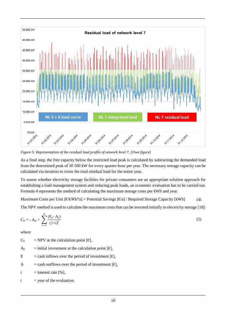
Since at network level 7, changes in the load behaviour should be evaluated, the load curves of network levels

5 and 6 do not vary during the study. The peak load of the combined load profile is set to maximum load level

that should be demanded. As the next step, the combined load profile is filled with the load profile of network

level 7 until the determined peak load. The residual load profile has to be covered by electricity storage. Figure

5 presents the residual load profile (red colour) of network level 7 on basis of real data from the practice partner.

The blue curve shows the combined load profile of network levels 5 and 6 with a peak load of 30 500 kW. The

filled up part of the network level 7 load is displayed in green. It can be clearly seen that a difference exists

between the load demand during the week (high demand) and on the week-ends (lower demand) at network

levels 5 and 6.

Network level ∑ 6 851 100 € ∑ 1 267 500 €

NL 5 A1 3 428 800 € B1 717 500 €

NL 6 A2 646 600 € B2 223 700 €

NL 7 A3 2 775 700 € B3 326 300 € 3 102 000 €

870 300 €

4 146 300 €

8 118 600 €

Baseline of the grid costs for the pricing model

Total costs

(A)

Demand costs of the upstream

network level above MinLoad

(B)

Cost approach for the pricing

model

(A - B = C)

(3)

10

Figure 5: Representation of the residual load profile of network level 7. [Own figure]

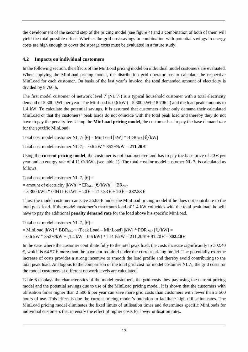
As a final step, the free capacity below the restricted load peak is calculated by subtracting the demanded load

from the determined peak of 30 500 kW for every quarter-hour per year. The necessary storage capacity can be

calculated via iteration to cover the total residual load for the entire year.

To assess whether electricity storage facilities for private consumers are an appropriate solution approach for

establishing a load management system and reducing peak loads, an economic evaluation has to be carried out.

Formula 4 represents the method of calculating the maximum storage costs per kWh and year.

Maximum Costs per Unit [€/kWh*a] = Potential Savings [€/a] / Required Storage Capacity [kWh]

The NPV method is used to calculate the maximum costs that can be invested initially in electricity storage [18]:

C0 = - A0 + ∑(Et- At)

(1+i)t

n

t =1

where

C0 = NPV at the calculation point [€],

A0 = initial investment at the calculation point [€],

E = cash inflows over the period of investment [€],

A = cash outflows over the period of investment [€],

i = interest rate [%],

t = year of the evaluation.

(4)

(5)

11

Based on the general life-cycle for batteries determined in the depreciation list [19], the observation period is

10 years. Taking the current low-interest phase into account, the interest rate of 2.5 % for the calculation is

assumed. The initial investment in a storage system is not known. Instead, the NPV is defined as zero to calculate

the maximum possible investment costs that can be paid while the investment is still positive.

4 Results

The following section presents the results of applying the developed pricing model and storage-based load man-

agement system. After evaluating the effects of the pricing scheme on distribution grid operator’s customers,

the effects on the overall system are the focus of the study.

4.1 MinLoad pricing model

Applying the methods described in section 2, the following pricing model is the result of the study. The used

data on grid costs are based on the profit and loss accounts of 2014, which was the last completed business year

at the beginning of the research project. Appropriately, the underlying data on load behaviour also originate

2014. The costs of the upstream network level (NL 4) were modified to the current cost level because of the

significant increase in costs over the last years. Compared to 2016, the demand rate that the practice partner has

to pay to the transmission grid operator is 56 % higher in 2017. Hence, 114 €/kW is defined as the penalty

demand rate, which is equivalent to the demand rate of network level 4. As represented in table 5, the base

demand rate varies from 143 €/kW for customers at network level 5 to 352 €/kW for customers at network level

7. Customers at network level 6 pay 155 €/kW as BDR. As mentioned before, the MinLoad pricing model

eliminates the base price as well as energy rate as tariff components compared to the current pricing model.

Table 5: MinLoad pricing scheme. [Own figure]

The significantly higher BDR at network level 7 results from the low MinLoad, which represents the low utili-

sation rate. The incentive to reduce peak loads is therefore the highest for household customers. This is in line

with the idea of the storage-based load management system at network level 7. In contrast to the current pricing

model, the MinLoad model eliminates the distinction between different utilisation times (more or less than

2 500 h per year). Legislators intended this differentiation to increase the utilisation time as well. Due to the

penalty fee, the requirement that customers who actually cause the peak load paying for the effect is significantly

stronger within the MinLoad pricing model. On the other hand, the cost-by-cause allocation of grid costs pre-

vents mutual subsidising by different customers.

As described in section 3.3, electricity storage at network level 7 represents the surmised load management

system reaching the planned peak-load reduction. It is assumed that changes in consumer behaviour concerning

Respective grid

costs

(A)

Respective

MinLoad

(B)

MinLoad Price

(A/B = C)Penalty Fee

Network level

NL 5 4 146 300 € 18 895 kW 143 €/kW 114 €/kW

NL 6 870 300 € 2 730 kW 155 €/kW 114 €/kW

NL 7 3 102 000 € 6 963 kW 352 €/kW 114 €/kW

∑ 8 118 600 € 28 588 kW 195 €/kW 114 €/kW

MinLoad pricing scheme

12

energy efficiency will only occur via technological instruments without waiving convenience aspects [20]. Con-

sequently, the prerequisite for electrical household appliances capable of load controlling (washing machines,

tumble dryers, dishwashers, etc.) is that they are equipped with automatic control units. The charge state of the

storage is used as behaviour-guiding information for the automatic household appliances and the consumer as

well.

To calculate the required capacity of the storage, one correspondingly large electricity storage capacity is as-

sumed for a first estimation. The determined peak load of the combined load profile of network levels 5 and 6

is 30 500 kW (see section 3.3). The peak load of the residual load profile of network level 7 amounts to 13

600 kW. If the total peak load can be covered by storage and thereby reduces the overall load peak accordingly,

the annual grid costs will decrease by 1 550 400 € [= 13 600 kW * 114 €/kW (PDR)]. According to the storage

model, a storage capacity of 2 970 000 kWh is necessary to cover the total residual load profile. Using the NPV

method, the maximum possible initial investment can be calculated as described in formula 5:

C0 = - A0 + ∑(Et- At)

(1+i)t

n

t =1

For the calculation of the initial investment the NPV is defined as zero:

A0 = ∑(Et- At)

(1+i)t

n

t =1

Using the determined interest rate of 2.5 % and life-cycle of 10 years, the initial investment is calculated as

follows:

A0 = 1 550 400 € * (1.025)-1 + 1 550 400 € * (1.025)-2 + 1 550 400 € * (1.025)-3 + 1 550 400 € * (1.025)-4 +

1 550 400 € * (1.025)-5 + 1 550 400 € * (1.025)-6 + 1 550 400 € * (1.025)-7 + 1 550 400 € * (1.025)-8 + 1 550 400 €

* (1.025)-9 + 1 550 400 € * (1.025)-10 = 13 569 200 €

The calculation shows that 13 569 200 € can be invested in the storage system at the moment to achieve the

peak-load reduction. By using formula 4, the maximum possible storage costs per unit can be calculated as

follows:

Maximum Costs per Unit [€/kWh] = Potential Savings [€] / Necessary Storage Capacity [kWh]

Maximum Costs per Unit = 13 569 200 € / 2 970 000 kWh = 4.57 €/kWh

It appears that a maximum initial investment of 4.57 €/kWh is significantly too little compared to the current

average market prices of 361 €/kWh – 1 044 €/kWh [21 - 22] for electricity storage. But it is important to keep

in mind that only saved grid costs have been taken into account, but not reduced energy costs and possible state

subsidies.

The first result of the storage evaluation is that it is extremely expensive for a storage system to cover the total

peak load due to the high storage capacity required. However, in the case of the practice partner, annual savings

of 1 550 400 € can be achieved by reducing peak loads at the network level 7. A smaller storage system in

combination with a power production system (e.g. emergency generators or cogeneration plants) could serve as

an alternative load management system. If, for instance, merely 80 % of the peak load should be covered by the

storage facilities, a capacity of 441 000 kWh is sufficient. The remaining 20 % of the peak load must be pro-

duced by an emergency generator, for example. As a result, the maximum initial investment increases signifi-

cantly. However, costs for the emergency generator are incurred. Nonetheless, one has to keep in mind that the

calculation of potential savings only relates to the grid costs. Energy costs are not taken into account. Hence,

13

the development of the second step of the pricing model (see figure 4) and a combination of both of them will

yield the total possible effect. Whether the grid cost savings in combination with potential savings in energy

costs are high enough to cover the storage costs must be evaluated in a future study.

4.2 Impacts on individual customers

In the following section, the effects of the MinLoad pricing model on individual model customers are evaluated.

When applying the MinLoad pricing model, the distribution grid operator has to calculate the respective

MinLoad for each customer. On basis of the last year’s invoice, the total demanded amount of electricity is

divided by 8 760 h.

The first model customer of network level 7 (NL 71) is a typical household customer with a total electricity

demand of 5 300 kWh per year. The MinLoad is 0.6 kW (= 5 300 kWh / 8 706 h) and the load peak amounts to

1.4 kW. To calculate the potential savings, it is assumed that customers either only demand their calculated

MinLoad or that the customers’ peak loads do not coincide with the total peak load and thereby they do not

have to pay the penalty fee. Using the MinLoad pricing model, the customer has to pay the base demand rate

for the specific MinLoad:

Total cost model customer NL 71 [€] = MinLoad [kW] * BDRNL7 [€/kW]

Total cost model customer NL 71 = 0.6 kW * 352 €/kW = 211.20 €

Using the current pricing model, the customer is not load metered and has to pay the base price of 20 € per

year and an energy rate of 4.11 Ct/kWh (see table 1). The total cost for model customer NL 71 is calculated as

follows:

Total cost model customer NL 71 [€] =

= amount of electricity [kWh] * ERNL7 [€/kWh] + BRNL7

= 5 300 kWh * 0.0411 €/kWh + 20 € = 217.83 € + 20 € = 237.83 €

Thus, the model customer can save 26.63 € under the MinLoad pricing model if he does not contribute to the

total peak load. If the model customer’s maximum load of 1.4 kW coincides with the total peak load, he will

have to pay the additional penalty demand rate for the load above his specific MinLoad.

Total cost model customer NL 71 [€] =

= MinLoad [kW] * BDRNL7 + (Peak Load – MinLoad) [kW] * PDR NL7 [€/kW] =

= 0.6 kW * 352 €/kW + (1.4 kW – 0.6 kW) * 114 €/kW = 211.20 € + 91.20 € = 302.40 €

In the case where the customer contribute fully to the total peak load, the costs increase significantly to 302.40

€, which is 64.57 € more than the payment required under the current pricing model. The potentially extreme

increase of costs provides a strong incentive to smooth the load profile and thereby avoid contributing to the

total peak load. Analogous to the comparison of the total grid cost for model costumer NL71, the grid costs for

the model customers at different network levels are calculated.

Table 6 displays the characteristics of the model customers, the grid costs they pay using the current pricing

model and the potential savings due to use of the MinLoad pricing model. It is shown that the customers with

utilisation times higher than 2 500 h per year can save more grid costs than customers with fewer than 2 500

hours of use. This effect is due the current pricing model’s intention to facilitate high utilisation rates. The

MinLoad pricing model eliminates the fixed limits of utilisation times and determines specific MinLoads for

individual customers that intensify the effect of higher costs for lower utilisation rates.

14

Table 6: Potential savings of the model customers due to the MinLoad pricing scheme compared to the current pricing

model. [Own figure]

Table 6 also shows that customers with the same MinLoad pay the same base demand rate. The differentiation

between the demand rates arises if the individual customer contributes to the total peak of the whole distribution

grid. As mentioned before, the MinLoad pricing model allocates the additional grid costs caused by a higher

total peak load to the responsible customers. The blue in figure 6 shows the potentially low grid costs (BDR)

that customers will pay if they achieve the peak reduction. The orange bar represents the maximum penalty fee

costumers will pay if they contribute fully to the total peak load. The incentive to reduce the respective peak

load is obvious.

Figure 6: Difference between the Base Demand Rate (BDR) and the Penalty Demand Rate (PDR) for the selected model

customers. [Own figure]

In summary, the second result is that in general, the MinLoad pricing model incentivises customers to reduce

their peak loads and to smooth their load profiles. Under the MinLoad pricing model, customers will directly

decrease their grid costs if they do not contribute (fully) to the total load peak. However, the peak-causing

Network

level

Model

customer

Annual

utilization time

Annual amount

of electricity Peak load MinLoad

Current

Pricing Model

MinLoad

Pricing Model

Potential

savings

NL51 >= 2 500 h/a 959 207 kWh 1 210 kW 109 kW 100 109 € 15 712 € 84 397 €

NL52 < 2 500 h/a 959 207 kWh 1 210 kW 109 kW 38 620 € 15 712 € 22 908 €

NL61 >= 2 500 h/a 283 378 kWh 290 kW 32 kW 25 800 € 5 012 € 20 788 €

NL62 < 2 500 h/a 283 378 kWh 290 kW 32 kW 11 950 € 5 012 € 6 938 €

NL72 >= 2 500 h/a 143 680 kWh 110 kW 16 kW 9 826 € 5 770 € 4 056 €

NL73 < 2 500 h/a 143 680 kWh 110 kW 16 kW 5 934 € 5 770 € 164 €

NL 5

NL 6

NL 7

Potential savings of the model customers

15

customers have to bear the incurred costs following the ‘polluter pays principle’. Using electricity storages as

load management measure provides the advantage of providing direct behaviour-guiding information to achieve

peak reduction. Considering that at present, the costs for electricity storage will exceed the saved grid costs,

alternative load management measures could be more attractive. Commercial customers in the food sector could

for example invest in new cooling technologies, which provide load management applications [23]. Moreover,

joint load management measures by industrial customers and respective distribution grid operators could also

be worth consideration to boost saving potentials. By implementing the MinLoad pricing model with significant

incentives to reduce peak loads, the most efficient technologies (or a combination of a number of technologies)

will emerge over a period of time.

4.3 Impacts on the overall system

The developed pricing model enables the realisation of the calculated potential savings and cost-by-cause allo-

cation of grid costs. On the transmission system operator side (NL 4), a deficit occurs in accordance with lower

grid charge revenues if the peak load can be reduced. If the maximum calculated load reduction of 13 600 kW

(see section 3.3) can be achieved by customers, the revenues of the network level 4 operator will decrease by

1 550 400 € [= 13 600 kW * 114 €/kW] per year. With a delay of two years, the transmission grid operator is

authorised - according to the regulatory laws in force [8] - to allocate the missing amount to the generality of

grid users in terms of increasing grid charges. Although the total costs of the transmission grid remain the same

(5 027 400 €), the peak load decreases from 44 100 kW to 30 500 kW. Hence, grid costs must be divided by the

reduced peak load. The price per unit increases from 114 €/kW to 165 €/kW [= 5 027 400 € / 30 500 kW]. As a

result, individual customers’ potential savings decrease on the one hand, whereas the incentive to reduce the

annual peak load increases. Over time, this combination leads to potential savings approaching zero in analogy

to the results of the preliminary study.

Consequently, the third result is that the pricing model needs to apply a two-step approach. In the first step, the

network costs can be the regulator of the load management system. In the second step, the costs of generating

electricity have to be focused to reach the shown goals as displayed in figure 4.

5 Conclusion

In summary, the advantages of the MinLoad pricing model are as follows: Due to an increase in utilisation rate

of the existing grid infrastructure, a reduction of grid costs per unit can be achieved. Moreover, future price

increases can be kept at a lower level because of a reduction in the necessary grid expansion. Since grid expan-

sions at higher network levels are planned [24], increased grid charges at higher network levels must be ex-

pected. As part of the end-user electricity price, higher transmission grid costs will affect the generality of

network users. Using the MinLoad pricing model enables distribution grid operators to create a locational ad-

vantage for the region in which they operate due to lower distribution grid costs at minimum. Furthermore, the

objective of allocating grid costs in accordance with the polluter can be achieved. Customers will pay for the

network costs they cause. However, the result is also that an exclusive storage-based load management system

cannot be financed solely by the saved grid costs at present. Covering the total residual peak load is extremely

expensive. A combination of different load management measures on both the demand and production sides

can be a more practicable approach. Due to the impending penalty fees, the implementation of the MinLoad

pricing model will foster the development of efficient load management measures and technologies. If the elec-

tricity storage-based load management system is economically possible, power production will become more

16

flexible, with increased fluctuations. This effect facilitates better integration of renewable energies into the elec-

tricity grids.

The next step of the research project will be the development of the second part of the pricing model, which

takes the production side into account. It is also necessary to analyse the interdependencies between the two

parts of the pricing model. Predominantly, the question to be answered is how implementation of both the in-

frastructure tariff components and energy price can operate in sync. Within a comprehensive study, the eco-

nomic equilibrium of grid expansion and load management technologies like storage has to be found. However,

advanced and appropriate data on electricity storage (costs and technical potentials) are required for such an

examination. Moreover, the within the preliminary study, elaborated interdependencies between the potential

savings of individual customers (groups) on the one hand and the generality of customers within the distribution

grid operator’s supply area on the other hand apply by analogy to the individual distribution grid operator and

generality of distribution grid operators within one supply network area. Identifying the impacts of the pricing

model on the upstream network levels will be part of a subsequent analysis.

It can be concluded that the implementation of a pricing model like the MinLoad pricing system requires an

intelligent grid including smart meters and smart home applications. Flexibility is the order of the day, as Auer

& Haas also argued in their recent paper [3].

References

[1] Federal Ministry of Economics and Technology (2010): Energiekonzept für eine umweltschonende, zuverlässige und

bezahlbare Energieversorgung. Berlin: Federal Ministry of Economics and Technology (ed.).

[2] Atomgesetz in the version of 15 July 1985 (BGBl. I p. 1565) last amended by Article 1 of the law of 1 June 2017

(BGBl. I p. 1434); Online at: https://www.gesetze-im-internet.de/atg/BJNR008140959.html (State: 20 June 2017).

[3] Auer, H., Haas, R. (2016): On integrating large shares of variable renewables into the electricity system. Energy 115

(2016), 1592 – 1601.

[4] Eid, C., Koliou, E., Valles, M., Reneses, J., Hakvoort, R. (2016): Time-based pricing and electricity demand response:

Existing barriers and next steps. Utilities Policy 40 (2016), 15 – 25.

[5] Stromnetzzugangsverordnung in the version of 25 July 2005 (BGBl. I p. 2243) last amended by Article 5 of the law of

29 August 2016 (BGBl. I p. 2034); Online at: http://www.gesetze-im-internet.de/stromnzv/BJNR224300005.html (State:

20 June 2017).

[6] Stromnetzentgeltverordnung in the version of 25 July 2005 (BGBl. I p. 2225) last amended by Article 8 of the law of

22 December 2016 (BGBl. I p. 3106); Online at: http://www.gesetze-im-internet.de/stromnev/BJNR222500005.html

(State: 20 June 2017).

[7] Gruber, M., Röder, H., Haber, A., Mayer, W. (2017): Load Management at Distribution Grid Level: Potential Savings

for Customers and Grid Operators? A German Example. 10. Internationale Energiewirtschaftstagung – Technische Uni-

versität Wien, Österreich, 15. – 17. Februar 2017. (German language)

[8] Anreizregulierungsverordnung in the version of 29 October 2007 (BGBl. I p. 2529) last amended by Article 1 of the

ordinance of 14 September 2016 (BGBl. I p. 2147); Online at: https://www.gesetze-im-inter-

net.de/aregv/BJNR252910007.html (State: 20 June 2017).

[9] European Commission (2014): Report from the commission: Benchmarking smart metering deployment in the EU-27

with a focus on electricity. Brussels: European Commission (ed.).

[10] Endres, A. (2011): Environmental Economics. Theory and Policy. New York: Cambridge University Press.

17

[11] Organisation for Economic Co-Operation and Development (OECD) (1992): The Polluter-Pays Principle: OECD

Analysis and Recommendations. Paris: OECD Publishing.

[12] Tonne, C., Beevers, S., Armstrong, B., Kelly, F., Wilinson, P., (2008): Air pollution and mortality benefits of the

London Congestion Charge: spatial and socioeconomic inequalities. Occupational and Environmental Medicine 65 (9),

620–627.

[13] Nelson, T., Orton, F. (2013): A new approach to congestion pricing in electricity markets: Improving user pays pricing

incentives. Energy Economics 40 (2013), 1 – 7.

[14] U.S. Department of Energy (2006): Benefits of Demand Response in Electricity Markets and Recommendations for

Achieving Them. A Report to the United States Congress Pusuant to Section 1252 of the Energy Policy Act of 2005.

Washington DC: U.S. Department of Energy (ed.).

[15] Faruqui, A., Sergici, S., Sharif, A. (2010): The impact of informational feedback on energy consumption - A survey

of the experimental evidence. Energy 35 (2010), 1598 – 1608.

[16] Faruqui, A., Hledik, R., Sergici, S. (2010): Piloting the smart grid. The Electricity Journal 22 (7), 55–69.

[17] Sensfuß, F., Ragwitz, M., Genoese, M. (2008): The merit-order effect: A detailed analysis of the price effect of re-

newable electricity generation on spot market prices in Germany. Energy Policy 36 (8), 3086-3094.

[18] Erdmann, G., Zweifel, P. (2010): Energieökonomik. Theorie und Anwendungen. Berlin: Springer-Verlag.

[19] German Federal Ministry of Finance (2000): AfA-Tabelle für die allgemein verwendbaren Anlagegüter. Berlin: Fed-

eral Ministry of Finance (ed.).

[20] Poortinga, W., Steg, L., Vlek, C., Wiersma, G. (2003): Household preferences for energy-saving measures: A conjoint

analysis. Journal of Economic Psychology 24(1), 49 – 64.

[21] Nykvist, B., Nilsson, M. (2015): Rapidly falling costs of battery packs for electric vehicles. Nature Climate Change

(5), 329–332.

[22] Setzermann, T. (2017): Preisvergleichsliste Batteriespeichersysteme bei TST. Online at: http://www.solarladen.de/tst-

pv-produkte/preisvergleich/speichersysteme (State: 28 June 2017).

[23] Becker, G. (2009): Elektrischer Spitzenlastausgleich in Lebensmittelketten. Strategien zur Verbesserung der Energie-

effizienz. Wieselburg: Austrian Federal Ministry of Transport, Innovation and Technology (ed.).

[24] Federal Network Agency (2017): EnLAG-Monitoring: Stand der Vorhaben aus dem Energieleitungsausbaugesetz

(EnLAG) nach dem ersten Quartal 2017. Bonn: Federal Network Agency (ed.).